A cross-country econometric analysis of the effect of disruptive

firms on mobile pricing

Research Document

Publication date: 15/03/2016

About this document In markets with relatively few large competing firms, there is a risk of consumer harm. This market structure is prevalent in the communications sector. Ofcom has undertaken this study to understand how such a market might be affected by one firm acting as a ‘disruptive’ operator.

Consumer harm in concentrated markets can arise even without a single dominant company or companies engaging in overt collusion. It may take the form of prices being substantially above costs or product quality being low. These problems can be exacerbated where takeovers or mergers lead to even fewer, bigger network operators.

Mobile communications is an industry which has historically been associated with a number of disruptive firms. In addition, in recent years there has been a trend of mergers and consolidation in mobile markets, some of which have involved so-called disruptive firms.

So Ofcom wanted to test a starting hypothesis that disruptive firms (which do not follow the crowd and actively disturb existing market dynamics) may act as an important competitive constraint where there is a limited number of large firms in a market; and that mergers or takeovers involving a disruptive firm, can reduce that competitive constraint to the detriment of consumers.

To test our starting hypothesis, we undertook a cross-country econometric study to examine the effects on pricing of disruptive firms in the mobile markets of a group of countries. Our statistical analysis compares mobile prices across twenty-five countries over the period 2010-2015, controlling for characteristics of differentiated mobile tariffs and country-specific effects.

Our findings support the proposition that disruptive firms reduce prices in the markets in which they operate. They also support the proposition that greater competition – delivered by a greater number of players – has a positive effect on pricing.

Contents

Section Page

1 Introduction 1

2 Disruptive firms 3

3 Approach 6

4 Data 10

5 Results 15

6 Potential Limitations 19

Annex Page

1. Data included in our analysis 26

2 Identifying disruptive firms 28

3 Estimation results 32

4 Robustness testing 37

1

Section 1

1 Introduction

What’s this all about?

What makes markets competitive? We know that a variety of factors influence the competitive dynamics in different markets at different times.

Under certain market conditions, firms can collude or co-ordinate so as to behave in an anti-competitive manner. For example, firms may raise prices above the competitive level, or they may offer lower quality products than they otherwise would. There may also be circumstances where oligopolistic market structures mean that competitive constraints among a small number of firms may be weak but the conditions for tacit collusion1 do not arise. In this latter case, individual firms may be acting in an economically rational manner which is not aimed at weakening competition but the consequences of those actions may be that competition is weakened to the detriment of consumers. In these circumstances, disruption, or even the threat of disruption to a market, can provide a spur to competition, and promote competitive rivalry amongst existing players.2

Generally, disruptive players (that do not follow the crowd and actively disturb existing market dynamics) have been seen by regulatory authorities as having a positive effect on markets for their ability to increase competition, with policies to encourage disruptive entry commonly explored. In addition, competition authorities have sometimes paid particular attention to disruptive players or “maverick” competitors in their decisions, for example, on mergers.3

Mobile communications is an industry which has historically been associated with a number of disruptive firms (for example, H3G in the UK and Free in France). In the context of the recent trend towards consolidation in European mobile markets, we are therefore interested in studying the effect of disruptive firms on competition.

Recent mergers in both Ireland and Austria have led to concerns in some quarters that these markets are losing their disruptive influences (H3G in both cases), ultimately to the detriment of consumers through either higher prices or dampened innovation4. Another view is that consolidation in European markets is necessary to ensure continued investment in the face of declining mobile revenues5,6. In this study, we do not test for the impact of disruptive firms

1 This is where firms within a market compete less aggressively with each other (for example, by avoiding the

opportunity to reduce prices) without explicitly agreeing to do so. 2 See, “Mavericks, mergers, and exclusion: proving coordinated competitive effects under the antitrust laws”, J

B Baker (April 2002), New York University Law Review, Vol 77 pp135 – 203. While Baker’s paper is in the context of coordinated effects, we consider that unilateral effects can also cause harm and the presence of a disruptive or maverick firm has the same significance in this context 3 One example is the EC’s decision on the Orange/T-Mobile merger in the UK, where particular attention was

paid to the effect on Three, the “maverick” competitor. 4 A study by the Austrian national regulator, RTR, finds that prices have increased for mobile users in Austria

following the merger between H3G and Orange in 2012 (particularly for ‘low power’ users). See - RTR Telekom Monitor (April 2015) (page 16) or RTR Telekom Monitor data (2015) (under tab “Mobilfunk”). 5 A report for the GSMA by Frontier Economics considers that mergers can increase unilateral incentives to

invest, finding that there is no clear link between competition and investment in three versus four player markets. See - Assessing the case for in-country mobile consolidation (May 2015)

Page Heading

2

(or the number of firms) on investment incentives but we do appreciate that the sustainability of disruptive strategies must also be considered.7

What are our main findings?

In analysing the effect of disruptive firms on competition, we undertake a cross-country econometric study to examine the effects on pricing of what we define as, disruptive firms in the mobile markets of a group of countries. Our econometric analysis compares mobile prices across twenty-five countries between 2010 and 2015, controlling for the characteristics of differentiated mobile tariffs and country-specific factors. In countries where a disruptive player is present, our analysis suggests (with a 95% confidence interval) that prices are lower of the order of between 10.7% and 12.4% compared to countries where a disruptive firm is not present.

Our analysis also indicates (with a 95% confidence interval) that prices are lower of the order of between 7.3% and 9.2% in countries where there are a greater number of players. Combining these two variables suggests that prices could be between 17.2% and 20.5%8 lower on average in countries where there are four or more mobile operators AND a disruptive firm is in the market.

While we appreciate that there may be a number of potential limitations with the analysis, our findings (subject to the caveats we set out below) support the proposition that disruptive firms reduce prices in the markets in which they operate. They also support the proposition that greater competition – delivered by a greater number of players – tends to reduce prices which is likely to benefit consumers.

The outline of this paper is as follows:

Section 2 provides a discussion of disruptive firms;

Section 3 sets out the approach that we use in this paper;

Section 4 describes the data and drawing from Section 2 sets out the criteria we use to identify disruptive firms in our sample;

We present our results in Section 5; and

In Section 6, we discuss potential limitations of this analysis.

6 HSBC considers that four to three mobile mergers would allow firms to increase their EBITDA margins (to

around 38%) so that they are able to invest more. See - Supersonic (April 2015) 7 We note that a firm’s disruptive strategy should not be assumed to be maintained over time. In the long run,

a previously disruptive firm may wish to act less aggressively once it has grown its market share sufficiently – see discussion in Section 2. 8 There is a multiplicative effect of combining the percentage values for the number of operators and

disruptive firms effects. This is explain in Section 5

3

Section 2

2 Disruptive firms

Our interest in disruption stems from the benefits it can bring to the market

We are interested in market disruption because of the effect it can have on competitive intensity in a market. Under certain conditions, markets may reach undesirable outcomes where prices are substantially above costs and/or product quality is low, even without a single dominant firm or players engaging in overtly collusive behaviour. This may be the case in markets with relatively few large competing firms, a market structure that is prevalent in the communications sector. Disruption, or even the threat of disruption, can disturb these market dynamics and promote competitive rivalry amongst players, ultimately to the benefit of consumers.

We consider that market disruption can arise for a number of reasons – see discussion below. National regulatory authorities can create the right conditions for it to emerge or continue through merger control, removing entry barriers, preventing strategic responses from incumbents etc. but these are all things we would do anyway to promote competition more generally.

Disruption is a strategic choice made by firms and is something that happens exogenously. However, once it emerges, we are keen to protect disruption to retain the consumer benefits associated with it. These benefits may take the form of lower retail prices or improved product offerings.

We recognise, however, that we need to remain mindful of any potential negative effects of disruption. For example, it may impact investment incentives if the threat of losing market share to the disruptor reduces the expected return on an investment for an incumbent firm.

Alternatively, the threat of disruption may, in fact, incentivise investment because if one player is willing to disrupt and bring new innovations and technical developments to market, rivals are likely to want to keep up, to remain competitive. This could introduce greater competition for access to new innovations and incentivise more investment in R&D. The overall effect may be to create conditions that are more conducive to innovation.

Ultimately, our view is that a level of disruption which encourages firms to invest and remain competitive in the market is likely to maximise the benefits to consumers in the long term. In this study, we do not test for the impact of disruptive firms (or the number of firms) on investment incentives but we do appreciate that the impact of disruption on the sustainability of investment is a consideration.

Page Heading

4

It is not easy to establish a catch-all definition of disruption

Disruption is often much easier to recognise than it is to define. Examples of disruptive firms and products exist in both communications and more generally in other markets e.g. EasyJet, Skype, Amazon, online news etc. We consider disruptive firms to disturb the existing market dynamics by doing or offering something different to that which already exists within the market. In doing so, they can provoke a reaction from competing firms. For example, Free’s entry in France drove the competing players to create spin-off brands to compete with Free and Bulldog’s offerings in the UK acted as a spur to BT to improve its own offerings.

Disruption is distinguished from other instances of entry or changes in strategy by the fact that it is not easily accommodated by competitors. Incumbent firms are likely to need to respond to the disruptive activity with non-trivial changes in strategy or business model, else they risk losing their position in the market. However, each case of disruption is usually unique, and it is this variation amongst disruptive firms which makes it difficult, if not impossible, to establish a rigid, catch-all definition of disruptive players.

Despite the difficulty of establishing a catch-all definition, there are some general behaviours and outcomes which we might consider to be common among many disruptive players: 9

a) Introduction of services which supersede others – the player innovates to offer a service which replaces existing offerings. An example may be emails replacing letters as a means of communication.

b) Introduction of new production technology for existing services – the player innovates to provide services that are comparable to those offered by competitors but with a technology that proves to be more productively efficient or provides a product with greater quality. An example may be digital as opposed to analogue television.

c) Aggressive behaviour – the player competes vigorously and prioritises gaining market share above other considerations such as profits or cost recovery in the short or even medium term.

In Section 4, we set out the behaviours and characteristics that we use to categorise firms as disruptive or otherwise for the narrower purpose of our analysis.

Disruption is often motivated by a drive for market share

We consider that disruption is generally motivated by a drive to increase market share to compete more effectively in a market. This is particularly likely to be the case in markets which display significant economies of scale where players can gain a competitive advantage by growing their customer base. However, once a disruptive firm has won enough customers, it may have little incentive to remain disruptive (unless it is subject to continued competitive pressure from other potentially disruptive firms)10. In this situation, it could then

make a commercial decision to act less disruptively because the incremental acquisition

9 It is important to note that while such characteristics may be common amongst some disruptors, their presence alone is not a sufficient condition for disruption and neither are they present in every case of disruption. 10

Christensen (1997) considers that once a firm reaches incumbency, they are less likely to act disruptively as they are incentivised to chase innovations with higher margins than those offered by potentially disruptive technologies. See Christensen, C. (1997), “The innovator’s dilemma; when new technologies cause great firms to fail”

5

costs of the marginal consumer and the risk of cannibalisation are likely to increase as the firm gains more market share. A similar incentive is likely to exist when a disruptive firm merges with a competitor, significantly increasing its market share. In this situation, there is a tension between disruption and the risk of cannibalisation of existing services. This may mean that to protect existing sales, the merged entity might have the incentive and ability to delay disruptive activities. If there is social value from disruptive activities, then from a societal perspective, this could lead to an inefficient outcome.

Mobile markets provide a good example of this. There are substantial fixed and sunk costs involved in building a mobile network (i.e. building of masts and investing in spectrum). Once a network is built, up to the available capacity, additional output can be produced at nearly zero marginal or incremental cost. Operators with small market shares will, therefore, initially have an incentive to quickly fill this capacity by competing aggressively for new customers which will help them to recover the fixed costs at a low marginal or incremental cost. However, once capacity gets close to being filled, the incentive may change so that the firm is less focused on building market share as it has less capacity available for new customers and a larger customer base to monetise.

Given the benefits that disruption can bring about, we need to be mindful of things that could undermine it. Although, we recognise the potential negative impact disruption can have on investment incentives, ultimately, a sustainable level of disruption that encourages firms to invest and remain competitive in the market is likely to maximise the benefits to consumers in the long term.

Page Heading

6

Section 3

3 Approach

We compare prices where a disruptive firm is present to those in markets where one is not

We note that a number of papers have recently been released which look to investigate the effect of mobile consolidation on prices11,12,13. A key difference between these studies and ours is that we have focused the analysis on the effect of disruptive firms rather than exclusively on changes in market concentration.

As set out above, in Section 2, under certain market conditions, oligopolistic market structures could foster undesirable outcomes where prices are substantially above costs and/or product quality is low. These undesirable outcomes can be exacerbated where there is consolidation of players in these already relatively concentrated markets. Disruption, or even the threat of disruption to a market, can disturb undesirable market dynamics and promote competitive rivalry amongst existing players, ultimately to the benefit of consumers. In this context, our starting hypothesis is that disruptive firms may act as an important competitive constraint where there is a limited number of competing firms in a market and that where consolidation involves a disruptive firm, this can lessen this constraint to the detriment of consumers.

Mobile communications is an industry which has historically been associated with a number of disruptive firms (for example, Free in France and H3G in the UK). In addition, in recent years there has been a trend towards consolidation in mobile markets, some of which have involved so-called disruptive firms. In the context of the recent trend towards consolidation in European mobile markets, we are therefore interested to test our starting hypothesis and consider the effect of disruptive firms on competition. Either prices or profits could be indicative of the level of competition.

Given the availability of data, we focus on prices such that we compare prices in national mobile markets where a disruptive firm is present to markets where one is not. If we find that prices are statistically significantly lower in markets with disruptive firms (all else being equal), we could take this as evidence that the presence of a disruptive firm provides a spur to competition which constrains prices within the national market in which it operates.

Hedonic pricing analysis allows for a like-for-like comparison of tariffs

Given the degree of differentiation in tariffs offered by mobile operators, it is difficult to simply directly compare their prices since they vary depending on the make-up of individual plans. To separate out quality differences and carry out a like-for-like comparison of tariffs, we use an estimation method called hedonic pricing analysis.

11

Evaluating Market Consolidation in Mobile Communications , Genakos, Valletti, and Verboven, September 2015. This considers the relationship between market concentration and prices (and investment), using tariff (but not handset) data. 12

“Assessing the Case for In-Country Mobile Consolidation: A Report Prepared for the GSMA”, Frontier Economics, May 2015, This considers the relationship between mergers and prices per megabyte of data (and investment) using ARPU data. 13

“Supersonic: European Telecoms Mergers will Boost Capex, Driving Prices Lower and Speeds Higher”, HSBC Global Research, April 2015. This study also considers the relationship between mergers and prices (using a unit price measure).

7

Hedonic pricing analysis has been used to compare the price of products whose quality changes over time or over the product space, due to either technological or subjective factors, or other services and optional equipment. It has been applied to many different products such as automobiles (Brenkers & Verboven, 200514; Berry, Levinsohn & Pakes, 199515 and 200416; Court, 193917; Griliches, 196118), wine (Haeger & Storchmann, 200619; Nerlove, 199520), housing (Maurer, Pitzer & Sebastian, 200421), PCs (Griliches, 199422; Pakes, 200323), mobile communications (Dewenter, Haucap, Luther & Rötzel, 200724), Internet service providers (Yu, 200125) etc.

The basic premise of the hedonic pricing method is that the value of a marketed good is related to its characteristics, or the services it provides. All else equal, higher quality products, with higher quality characteristics or services, will have higher prices. According to Lancaster’s (1971)26 theory of consumption, a product consists of various characteristics that consumers value. As a consequence, we can think of the product’s total price as being the sum of the prices derived from the value of each characteristic. The price of a certain characteristic is, therefore, regarded as a hedonic price so that a product’s total price may be decomposed into the product’s single characteristics’ prices, determining the consumer’s willingness to pay for each characteristic (Rosen, 197427). For example, the price of a car reflects the characteristics of that car - speed, comfort, style, luxury, fuel economy, etc. Therefore, the individual characteristics of a car or other good can be valued by looking at how the price people are willing to pay changes when the characteristics change.

The hedonic price method allows one to compare prices across products, across time or across countries by decomposing price differences into price differences that are accounted for by quality differences and those that are accounted for by changing market conditions. Thus, they enable one to compare prices on a like-for-like basis.

14

Brenkers, R. & Verboven, F. (2005). Market Definition with Differentiated Products - Lessons from the Car Market. CEPR Discussion Papers 5249, C.E.P.R. 15

Berry, S, Levinsohn, J, & Pakes, A. (1995). Automobile prices in market equilibrium. Econometrica, 63, 841-890 16

Berry, S, Levinsohn, J, & Pakes, A. (2004). Differentiated products demand systems from combination of micro and macro data: the new care market. Journal of Political Economy, 112, 68-105 17

Court, A. (1993). Hedonic price indexes with automotive examples. American Statistical Association (Ed.), “The dynamics of automobile demand”, 99-117, New York: General Motors Corporation 18

Griliches, Z. (1961). Hedonic price indexes for automobiles: An econometric analysis of quality change. NBER (eds.), The price statistics of the federal government, 173-196, New York: NBER 19

Haeger, J. & Storchmann, K. (2006). Prices of American Pinot Noir Wines: Climate, craftsmanship, critics. Agricultural Economics, 35, 67-78 20

Nerlove, M. (1995). Hedonic price functions and the measurement of preferences: the case of Swedish wine consumers. European Economic Review, 39, 1697-1716 21

Maurer, R., Pitzer, M. & Sebastian, S. (2004). Hedonic prices indices for the Paris housing market, Allgemeines Statistisches Archiv, 88, 303-326 22

Griliches, Z. (1994). Hedonic prices indexes for personal computers: intertemporal and interspatial comparisons. Economics Letters, 44, 353-357 23

Pakes, A. (2003). A reconsideration of hedonic price indexes with an application to PCs. American Economic Review, 93, 1578-1596 24

Dewenter, R., Haucap, J., Luther, R., & Rötzel, P. (2007). Hedonic prices in the German market for mobile phones. Telecommunications Policy, 31(1), 4-13 25

Yu, K. (2001). An Elementary Price Index for Internet Service Providers In Canada: A Hedonic Study (April 2001) Paper presented at the Sixth Meeting of the International Working Group on Price Indices Canberra, Australia 26

Lancaster, K. (1971). Consumer demand. New York: Columbia University Press 27

Rosen, S (1974), “Hedonic prices and implicit markets”, Journal of Political Economy, 82, 34-55

Page Heading

8

The hedonic price method is a particular kind of regression analysis that essentially involves decomposing the price into the constituent characteristics of a firm’s offering. To obtain estimates of the contributory value of each characteristic, we need to identify the relevant product features. When comparing the prices of two entities, it could be that the products of the best candidate have one special characteristic that no other product has. In other cases, it may be that it is the firm’s identity that could be unique – the contributory value of this can be determined by a firm’s dummy variable (Dewenter, Haucap, Luther & Rötzel, 200728). For example, relevant characteristics for our purposes in the context of mobile offerings may be minutes’ allowances, contract length, whether the plan is LTE-compatible, whether a disruptive firm is present, whether costs are high or low, how competitive the market is etc. More detail on this is set out in Section 4.

The typical hedonic relationship for a product offering and the hedonic regression corresponding to this function is:

p = f(X, β) + u (1)

where p is a vector of the price observations of the products i at time t where i = 1, …, n and t = 1, …, T, X is a matrix of characteristics’ vectors for product i at time t, β is a parameter vector that needs to be estimated and u is a vector of disturbance terms.

We estimate how much price changes if a disruptive firm is present versus if it is not

Using the data (discussed in the next section), we estimate a version of the following:

𝑝𝑖𝑜𝑐𝑡=𝛼𝑄𝑖𝑜𝑐𝑡 + 𝛽𝑡 + 𝛾𝑐𝑜 + 𝛿𝐶𝑐𝑡 + 𝜃𝐷𝑐𝑡 + 휀𝑖𝑜𝑐𝑡 (2)

Where 𝑝 is price, 𝑄𝑖𝑡 is a vector of quality variables related to each tariff observation 𝑖 at time 𝑡, 𝛽𝑡 is a year fixed effect, 𝛾𝑐 is a country-operator fixed effect, 𝐶𝑐𝑡 is a market concentration

dummy, 𝐷𝑐𝑡 is a dummy variable capturing the presence or not of a disruptive firm in country 𝑐 at time 𝑡, and 휀𝑖𝑜𝑐𝑡 is an error term for each tariff observation 𝑖, associated with an operator

𝑜, country 𝑐 and time 𝑡.

The resulting function measures the portion of the firms’ products’ prices that are attributable

to each characteristic. By looking at the hedonic price ctDp 29 we can get an estimate

of how much price 𝑝𝑖𝑜𝑐𝑡 changes if a disruptive firm is present in the market versus if it is not.

The hedonic pricing method is relatively straightforward to apply, because it is based on actual (or published) prices and product characteristics that are generally readily available. "Hedonics" is, however, not above criticism. All observations entering the regression equation have equal weight in determining the regression results as if they were of equal importance30. In addition, the relationship between price and the characteristics of the product may not be linear – prices may increase at an increasing or decreasing rate when

28

See footnote 24 29

This only holds if (1) is linear. We have assumed this notation and this functional form for the sake of simplicity. As noted further in the section, different functional forms should be tested when carrying out hedonic estimations. 30

We discuss this further in Section 6

9

characteristics change31. Moreover, many of the variables could be correlated, so that their values change in similar ways. In Section 6, we discuss potential limitations of this analysis.

31

We consider this in Section 5 and in Annex 4.

Page Heading

10

Section 4

4 Data In this section we describe some of the pertinent characteristics of mobile offerings that we consider in our analysis. We set out the data sources we have used for the analysis and discuss how we define disruptive firms for the purpose of constructing the variable we use to test for the effect of disruptive firms.

There are many relevant features of mobile offerings

The pricing strategies of MNOs are relatively complex compared to those of firms in many other industries. Operators vary their offerings along a number of lines in an attempt to capture as much of the heterogeneous tastes of consumers as possible; prices vary depending on the make-up of individual plans.

A significant factor which has an effect on mobile pricing is the length of the contract. All else being equal, a shorter contract is likely to be more expensive than a longer one as operators will look to incentivise consumers to sign up with them for a longer period of time.32

The handset which a consumer chooses is also an important factor. A wide variety of different handset makes and models are made available by operators on their pay monthly plans. A common strategy for MNOs is to offer a handset upfront for free and recoup the cost of the device via a monthly charge, over the period of the contract. However, in the case of more expensive handsets, MNOs also offer consumers the option of paying a one-off cost upfront and reducing the monthly payments accordingly. A number of papers have recently been released which have similarly looked to investigate the effect of mobile consolidation on prices33. Most exclude handset data. Given our view that the handset price is likely to be a key determinant of a mobile operator’s overall pricing decision, its inclusion is important to our study.

MNOs also offer monthly allowances of texts, data and minutes as part of their plans. These allowances are included as part of the mobile contract; the consumer only pays extra where they exceed the allowance. The larger these allowances are, the greater the cost of the contract, all else being equal. The total allowance of each factor and their mix vary between plans as MNOs attempt to shape their contracts to suit heterogeneous consumer demand.

There may also be quality considerations which further affect the prices that MNOs can charge. If consumers value the speed or coverage of a service, they may be willing to pay extra to receive services from that operator over others. For example, consumers may be willing to pay a premium to an operator which offers faster 4G services than they would for one which only offers 3G.

32

A possible alternative reason could be that price differences between contract lengths are driven by the recoupment of handset subsidies – i.e. expensive handsets are recouped over a long time period. We do not consider this to be the case as most contracts offered by MNOs are of similar lengths regardless of the handset being offered. More advanced handsets are paid back via a larger upfront and/or monthly fee rather than over a longer period of time. 33

See footnotes 11, 12, 13

11

Our data is publicly available information from Teligen and Tarifica

Given the pricing strategies of MNOs, we undertook to collect data on a number of key features of the mobile sector as described above. Many other studies of this nature exclude handset data because of a concern that a preference for handsets is being estimated rather than mobile tariffs. However, we believe handset pricing to be a key factor in an MNO’s pricing decision. As set out above, many MNOs subsidise handsets to make plans more attractive to consumers. This is an important element of their pricing decision and it could be that disruptive firms are more likely to aggressively pursue this strategy to expand their customer base. Given what we see as the inextricable link between handsets and tariff pricing, it seems important to us to include this effect in our analysis.

In light of the above, for the purpose of the analysis (as set out in Section 3), we collected data for twenty-five countries34 for the years 2010 to 2015. Collecting comprehensive data on mobile pricing plans and handsets from a single data source proved difficult. As such, we used two sources, Teligen and Tarifica: 35

a) Tarifica supplied us with data on post-paid mobile tariff plans. The data includes, for each pricing plan, information on monthly price, any connection fee, monthly minutes, texts and data allowances and any special features. This does not include pay-as-you-go plans because, unlike post-paid tariff plans, the prices consumers pay each month depend on their specific usage in that month. Since we do not have data on consumer usage of mobile services, we cannot capture this in our analysis.

b) Teligen provided us with information on the mobile handsets available for each tariff and the additional cost associated with buying them (if any). Given the large number of different handsets that are available per year, Teligen categorised the different handsets each year into three different categories: advanced, intermediate and basic. These handset categorisations are constant across countries but change over time. For example, a certain handset may be considered ‘advanced’ in one year but could be categorised as ‘intermediate’ two years later if its technology is superseded by another.

Teligen undertook the task of matching the data provided by Tarifica with its own data to produce a consolidated dataset36. This was done by using common keys such as plan names, years, and monthly price. In a number of instances, Teligen was unable to match

34

These countries are Australia, Austria, Belgium, Canada, Czech Republic, Denmark, Finland, France, Germany, Greece, Hong Kong, Ireland, Italy, Japan, Malaysia, Netherlands, New Zealand, Norway, Poland, Portugal, South Africa, Spain, Sweden, United Kingdom and United States. We note that the US displays some differences to other mobile markets in that it is made up of a number of smaller geographic markets – for consistency, we consider prices published at the national level by the four national operators in the US in our analysis. 35

Tarifica had comprehensive data on mobile pricing plans but did not have handset data. Teligen in contrast had handset data but it did not have comprehensive data on mobile pricing plans (in that the data only covers the largest two incumbent operators). 36

A potential criticism of this approach could be that matching tariff plans with handsets could lead to selection issues as the analysis may estimate preferences for handsets rather than mobile tariffs per se. As we set out previously, we do not see it this way. We consider that each combination of tariff plan and handset should be a unique observation since this is the choice that consumers face when they look to purchase a new mobile and plan. It is often the case that the price of a tariff plan changes with the type of handset, this effect would not be included in the analysis if it did not include handset data. While we consider it important to include handsets in our analysis, we do test for the effect on our results of not including them. This is discussed in Annex 4

Page Heading

12

Tarifica’s pricing plans with its own handset data. Some of the common reasons for this were:

a) There are exclusive online discounts which do not appear in one of either of the two datasets;

b) Financing has been bundled with a price in one of the datasets;

c) The contract lengths between the two datasets do not match up;

d) Plan prices (absent separate handset prices) between the two datasets do not match up;

e) There is an inconsistency between what a plan name implies and the data - for example, a Blackberry device matching a plan quoted as being iPhone-specific; or

f) There is a mismatch between the carriers covered in both datasets.37

Where a pricing plan does not match a handset plan (or vice versa), we have chosen to exclude that observation from our final dataset. In Section 6, we consider whether doing so has an impact on our analysis.

The consolidated database contains a number of other observations which we also disregard. These are:

a) Business plans – in this study, we are only interested in exploring the effect of disruptive firms on consumer tariffs.

b) Other devices – the data also include tariffs for dongles, wearable devices (i.e. smart watches) and tablets. We disregard all data that is not associated with mobile phones since this is the focus of our analysis.

c) Shared plans – we disregard plans which apply to more than one individual since they are generally more expensive and we are unable to allow for there being more than one plan user in the analysis. Since these plans are more prevalent in some countries than others, including them would likely bias the results.

Combining the datasets gives us a comprehensive set of data which is distinct from a number of of other studies (such as Genakos, Valletti and Verboven, 2015, HSBC, 2015, and Huongbonon, 201538) that use a dataset which only includes tariff data for the top two operators in a country. In addition, we focus on published mobile tariffs. Other analyses have taken different approaches to measuring price, such as using baskets to represent popular plans, estimating price per unit of mobile output39 and Average Revenue Per User (ARPU) .

37

The Teligen data does not include handset information for PCCW and Smartone in Hong Kong and includes limited data on T-Mobile in the Czech Republic and Vodacom in South Africa. Both sources started tracking some operators later than 2010 and, therefore, do not include data for them throughout all six years. 38

The Impact of Entry and Merger on the Price of Mobile Telecommunication Services, Huongbonon, G, V. (May 2015) 39

This has some similarities to an ARPU calculation but uses weights to mix together different outputs (i.e. data, voice minutes and texts) and converts them into megabytes. Total market revenues are then divided by this figure. The usual ARPU approach involves dividing revenues attributed to the consumption of mobile services by the number of SIM cards. We consider the unit price measure to be conceptually flawed as a metric of price changes or consumer welfare outcomes because it is not a measure of prices which are actually

13

After these transformations, we are left with 242,155 observations across twenty-five countries and six time periods. The data that we use in our analysis is discussed in more detail in Annex 1.

We identify disruptive firms using a number of features

As we discussed in Section 2, by its nature, defining whether a firm is disruptive or not is necessarily subjective as there is no catch-all definition. There are, however, some common characteristics which have been set out above.

In our classification of disruptive firms, they are much more than just price discounters. For example, they may be the first MNO in a market to offer unlimited data allowances, they may abolish roaming charges, they may bundle new services with their tariffs or they may be leaders in rolling out new infrastructure. The key feature though of disruptors is that other incumbent firms are likely to need to respond to the disruptive activity with non-trivial changes in strategy or business model, else they risk losing their position in the market.

In Section 2, we set out three broad behaviours and outcomes that may be consistent among disruptive firms. Here we apply these to the mobile market to determine relevant criteria to define disruptive firms. In light of this, using a mix of desk research and discussions with internal experts40 we look to categorise firms as disruptive or otherwise based on:

Introduction of services which supersede others

As we discuss in Section 2, firms can act disruptively by introducing new services that competitors do not and which cannot be easily accommodated by competitors. In such circumstances, incumbent firms may therefore need to respond to the disruptive activity. In mobile markets, examples of these may be being the first to offer unlimited data plans or abolish international roaming charges. In many instances, incumbent firms have been forced to respond by increasing their data allowances and reducing or abolishing their international roaming charges.

Introduction of new production technology for existing services

Players can also disrupt the market by using new technologies that are more productively efficient or provide products with greater quality. We consider that this is less relevant in mobile services because, historically, technical standards in mobile technology (i.e. LTE) have been developed at an international level, and being able to introduce new technology is very dependent on access to appropriate spectrum. We have, therefore, not identified any criteria based on this outcome.

Aggressive behaviour

A key feature of disruptive firms is their ability to compete vigorously and prioritise gaining market share above other considerations such as profits or cost recovery in the short or even medium term. Our view is that to do this, we should consider a number of criteria:

available to consumers and does not adequately reflect the complexity of mobile tariffs (such as differences between average and marginal prices). In addition, changes in ‘unit prices’ over recent years have been driven by increased data consumption which has been disproportionately related to a sub-set of consumers. 40

A number of these criteria have also been used in a 2012 report by Rewheel, see - Rewheel EU27 smartphone tariff competitiveness report - December 2012

Page Heading

14

The relative size of the operators – as we discuss in Section 2, disruption is often motivated by a drive to increase market share. MNOs with a low but significant market share (somewhere around 10%) are more likely to act as disruptive firms. This is because they are small enough to need to act aggressively to gain sufficient scale to compete with larger operators in markets with substantial economies of scale but are large enough to act as a viable competitive constraint on incumbent firms.

The parent groups which operators belong to – in general, MNOs belonging to large incumbent groups (such as Telefonica Group, France Telecom and Vodafone Group) are unlikely to be disruptive since the group-wide strategy in these organisations is not likely to be consistent with a disruptive strategy.41

Customer acquisition – we would expect a successfully disruptive firm to be able to acquire customers from rival firms as a result of its aggressive strategies or innovative offers. We would be unlikely to consider a firm which cannot acquire customers to be disruptive since this may imply that its strategy is not acting as a competitive constraint on incumbent firms.

General financial information – a firm must be in a stable financial position to allow it to pursue and maintain a disruptive strategy such as acting aggressively or creating innovative offerings over a period which is long enough to act as a constraint on incumbent firms. We note, though, that a firm may be able to sustain a loss where it has continued support from a wealthy backer (i.e. in the case of H3G).

Our categorisation of disruptive firms on this basis is set out in Annex 2. Analysis of our data shows that there are a number of similarities among these firms:

a) They are all of a similar size in relation to the market. They hold somewhere between 7 and 20% market share – most have around a 10% share. They, therefore, have sufficient scale to compete with larger operators and act as a competitive constraint. In addition, some have grown considerably over the period of the study. For example, Three UK had 4.9 million connections in 2009. This grew to more than 10.2 million by the end of 201442. This growth in size shows that they can demonstrate customer acquisition;

b) They tend to set prices at the lower end of the market, either being the cheapest or, sometimes, the second cheapest operator in a country. This is consistent with an aggressive strategy as set out above; and

c) They often offer larger contract allowances (in particular, data).

41

This is consistent with the work on disruptive innovation by Christensen, which considered that entrants are better placed than incumbents to embrace disruptive technologies as they are more willing to enter lower value market segments and have a lower risk of cannibalisation of existing offerings. See Christensen, C. (1997), “The innovator’s dilemma; when new technologies cause great firms to fail” 42

See - Ofcom, The Communications Market 2010 (page 321) and ft.com, Profits at Three climb by a third ahead of £10bn O2 merger

15

Section 5

5 Results

We run a pooled OLS on our data using a general-to-specific procedure to compare prices on a like-for-like basis

As set out in the previous section, the consolidated dataset comprises of 242,155 observations across twenty-five countries and six time periods. Given the approach that was adopted to match the two datasets, a number of observations were excluded. The effect of this is that we have an unbalanced dataset43, which means that it is not too distinct from a pooled cross-sectional analysis. A pure fixed effects estimation approach would not be an appropriate technique because it would not be able to take account of within observation variation over time. Given this, we run a pooled OLS on our data using a general-to-specific estimation procedure.44

As discussed in Section 3, a key consideration with hedonic analysis is that the relationship between price and the characteristics of the tariff plan many not be linear – prices may increase at an increasing or decreasing rate when characteristics change. On the basis of a test for selecting the most appropriate functional form and ease of interpretation, we use the natural logarithm of price and include a variable which is plan duration squared in our final specification. This is discussed further in Annex 4.

Our results are broadly consistent with what we would expect pre-estimation and our results are robust to a number of alternative specifications

The results reported in Table 1 exclude the country-operator dummies and allowance variables for simplicity. The full list of results for all variables in the specification is reported in Annex 3. As set out in Annex 4, we have estimated a number of alternative models. The results in Table 1 are robust to these.

Table 1: Estimation results (excluding country-operator dummies)45

Variable Coefficient estimate (t-statistic)

Adj. R-squared 0.992 RMSE 0.389 Basic handset -0.486 (-217.80) Intermediate handset -0.300 (-172.78) Plan duration -0.001 (-2.54) Plan duration squared -0.000 (-6.24) LTE -0.015 (-6.24)

43

It is an unbalanced dataset because tariff plans and handsets are often not present throughout the six years of our study - observations (which are country-operator-tariff combinations) are, therefore, often not available in all time periods. 44

The general-to-specific approach starts with a general statistical model that captures the essential characteristics of the underlying dataset. The general model is reduced in complexity by eliminating statistically insignificant variables, checking the validity of the reductions at every stage to ensure congruence of the finally selected model. This ensures that all important contributing variables are included in the final model specification. 45

Standard errors are corrected for autocorrelation by clustering by country-operator-tariff. This allows there to be correlation within observations (i.e. over a number of years for the same tariff plan) but not between observations.

Page Heading

16

2011 0.209 (14.95) 2012 0.284 (20.09) 2013 0.216 (15.40) 2014 0.171 (12.02) 2015 0.145 (10.15) Number of operators -0.082 (-16.40) Disruptive -0.123 (-24.23)

The results reported in Table 1 are broadly consistent with what we would expect pre-estimation. For example, they can be interpreted as showing that, on average:

a) prices are higher, the better quality handset associated with the plan;

b) longer plans are associated with slightly lower prices but as the duration of the plan increases, prices decrease at a diminishing rate. The result can be interpreted as indicating that, on average, a one unit (month) increase in contract length is associated with a 0.1% reduction in prices. Therefore, tariff prices will be 1.2% cheaper for each additional year of contract length; and

c) prices have fallen on average (since 2012)46.

The one potentially counter-intuitive result is associated with our LTE variable. This indicates that plans are approximately 1% cheaper, on average, when they are LTE-compatible compared to when they are not. We may usually expect the sign on this coefficient to be positive as operators charge more for better quality services. However, we consider there to be a number of reasons why this may not necessarily be the case:

a) Investment in LTE networks by operators may be used to compete more effectively with rivals rather than being used as a means to increase revenues.

b) It is expensive for MNOs to run parallel networks of different quality so operators may be incentivised to keep LTE prices down to incentivise consumers to move to the newer network so that they can reallocate resources (i.e. spectrum) to the newer technology quicker.

c) Customers using LTE networks consume more data than those using legacy technologies. MNOs may, therefore, look to increase their revenues by upselling customers to more expensive contracts, with larger data allowances, rather than increasing the prices of plans – keeping LTE prices low would encourage this. We cannot measure this effect because of a lack of demand data.

d) Rather than being seen by customers as being a vastly superior technology for which they expect to pay more, LTE could instead be seen as a necessary and expected upgrade to networks to keep pace with other technological developments (e.g. video streaming on mobile devices). If customers are not expecting to pay more for the transition to LTE, MNOs may not be able to justify price increases to them.

We consider that a combination of these factors mean our estimated coefficient for the LTE variable is not as unintuitive as it may initially seem.

46

We consider that the spike in prices in 2012 could be a lagged result of high global inflation in the previous year as higher costs fed through to mobile operators. See - statista.com

17

Prices are between 17.2% and 20.5% lower on average in countries where there is one additional mobile operator AND a disruptive firm is in the market

Given the focus of our study, the final two outputs of the estimation are of the most interest. The estimated value of the number of operators coefficient can be interpreted as indicating that prices decrease by approximately 8% on average when there is one additional (non-disruptive) operator present in a market.47 Based on a 95% confidence interval, this equates to prices being between 7.3% and 9.2% lower where there is one extra player in a mobile market.

Similarly, the estimated coefficient on the disruptive dummy can be interpreted as prices being approximately 12%48 lower on average in markets where a disruptive firm is present than in those where one is not. Based on a 95% confidence interval, this suggests that prices are between 10.7% and 12.4% lower where a disruptive firm is present.

Conbining the two sets of confidence intervals indicates that prices could be between 17.2% and 20.5%49 lower on average in countries where there are four or more mobile operators AND a disruptive firm is in the market. By implication, this may suggest that removing a disruptive player from a four player market (as is proposed in the H3G/O2 merger in the UK) could increase prices by between 17.2% and 20.5%% on average, all else being equal.

We have performed a number of robustness checks, which confirm our main findings

We have performed a number of robustness tests on the analysis which we set out in more detail in Annex 4. In summary, these tests are:

a) Test of a different specification – as we discuss above, on the basis of tests for selecting the most appropriate functional form, we included a squared explanatory variable in our estimation. We also test some other potential specifications. Our findings indicate that we should use the specification which includes a logged dependent variable and a squared explanatory variable.

b) Excluding handset data from the analysis – as we note above, a significant difference between our analysis and that of similar studies is that we include handset data in our estimation. As a check, we run a test which compares models with and without handset data. This test suggests that we should prefer the inclusion of handset data in our analysis.

47

This is comparable to the findings of Genakos, Valletti and Verboven (2015) who used a different dataset and approach to find that a reduction in the number of mobile operators would increase prices, on average, by 8.6%. 48

A crude interpretation of the disruptive dummy would be to simply assume an effect of -12% as this is how to interpret a linear variable in a log-linear equation. However, interpreting a dummy variable in a log-linear equation is different to interpreting a continuous variable. When interpreting a dummy variable in a log-linear regression, we must first take the exponential of both sides of our equation and then evaluate what the independent variable is when the dummy is equal to zero and when it is equal to one. The dummy should be interpreted as ‘if the variable switches from 0 to 1, the percentage impact of it on the dependent variable is equal to 100*(exp(output)-1).’ In other words, based on our estimated results, this would equate to 100 x [exp(-0.123)-1) = - 11.6% which we round up to -12% - this just happens to give the same value as the crude method described above. See, for example; Econometrics Beat: Dave Giles' Blog 49

There is a multiplicative effect of combining the percentage values for the number of operators and disruptive firms effects. For example, the lower 17.2% value is calculated as 1-[(1-0.107)*(1-0.073)] = 0.172.

Page Heading

18

c) Alternative methods of allowing for unlimited allowances – our data includes unlimited minutes, SMS, and data allowances which we cannot directly include in the analysis. We test to ensure that the way we include these factors (by describing them as categorical variables) does not bias the results. The results from doing this are not substantively different from where we use categorical variables so we decide to keep the original specification.

d) Tests of country-operator and year-specific factors to ensure that the results are not driven by the inclusion of data from any specific year or operator. We find that the results are not driven by data from any specific year or operator.

e) Tests of aspects of the pricing plans (for example, omitting all observations with unlimited data) to ensure that the results are not driven by data from any specific aspects of the pricing plans. We find that the results are not driven by data from any specific aspects of the pricing plans.

f) Tests of different categorisations of disruptive firms – as we discuss in Section 2, the categorisation of disruptive firms is necessarily subjective. We test to ensure that the analysis is robust to alternative (realistic) definitions of disruptive firms. Doing so has little impact on the main results so we consider the analysis to be robust to sensible variations in the categorisation of disruptive firms.

g) Test of a different concentration measure – an alternative way to allow for market concentration could be to include a dummy variable which measures whether there are three or four operators present in the market. This tests whether defining the market concentration variable in this way affects the analysis. The results of this test and the fit of the model are not substantially different from those of the main specification.

19

Section 6

6 Potential limitations This study is driven by data availability and therefore has some limitations. In the interests of academic robustness and transparency, we discuss these in this section. In particular, we discuss the following:

a) The lack of demand information

b) The potentially subjective nature of defining a disruptive firm dummy variable

c) The potential for endogeneity in the analysis

d) The handset categorisation used in this analysis

e) Data exclusion

We discuss these in turn below.

Lack of demand information

As discussed in Section 3, we look at the prices that MNOs set rather than what consumers demand. This is a necessity since data on consumer demand and usage are not readily available to us. The effect of this is that the analysis may suffer from the following two limitations: 50

All observations entering the regression equation have equal weight; and

The analysis does not consider over-use charges

Observations have equal weight

The lack of demand-side data means that we do not know the take-up of each plan in our dataset. This means that we necessarily give each tariff equal weighting whereas, in reality, it may be that in certain countries, one particular tariff is far more popular than others and should be given a larger weighting.

Consumers have quite diverse demand for mobile services so it makes sense that there should be a large variety of tariff plans available in a national market as operators look to

50 A further possible limitation is that our analysis cannot control for potential increases in consumer welfare which could arise when a consumer increases their data consumption within a given allowance. For example, a consumer may have a 2GB data allowance but consume 1GB in one year and 1.5GB in the subsequent year – thus benefiting more in the second year if they value consuming additional data. We do not consider this to be problematic for the purposes of our analysis since this simply tracks a trend in consumer usage over time which would likely occur regardless of any change in market concentration or the presence of a disruptive firm. This is different to the case where, for example, the entry of a disruptive firm increases the average data allowance in a market and some consumers, whose data consumption was previously price-constrained, subsequently increase their consumption of data. The latter example is relevant to the question of whether a disruptive firm (or market concentration) has an effect on consumers and will be picked up in the hedonic

pricing analysis whereas the first is not.

Page Heading

20

price discriminate based on differentiated consumer preferences. An approach to deal with this would be to weight the tariffs according to their popularity. However given data limitations, we are unable to do this.51

Our view is that the equal weight assumption is not a problem for estimating the parameters if the error term is uncorrelated with the regressors, that is if there is no endogeneity problem. As long as the error term, u, is uncorrelated with the regressors (i.e. endogeneity is not a problem), the lack of weighting should not therefore introduce bias into the analysis since the observed tariffs will be representative of all tariffs. Instead, not weighting tariff plans by take-up may mean that the results are less precise52. This is a less significant issue.

No consideration of over-use charges

The second possible limitation is that, since our analysis does not consider the extent to which customers exceed their contracted allowances and the effects of doing so, the monthly tariff price may not be equivalent to total bills in all cases. The analysis will, therefore, not be able to capture potential strategies where mobile operators include relatively limited allowances in their tariffs and rely on over-use charges to drive their revenues. If this was a strategy that was prevalent in some countries more than others, it might bias our results if over-use charges and the extent to which consumers exceeded their contracted limits were not included in the analysis. However, we do not consider this to be a significant problem for three reasons:

a) We do not have any information to suggest that this strategy might be prevalent in some countries more than others. Our analysis of out of allowance charges53 finds that there is no systematic difference in the level of these charges between countries (i.e., between those with and without a disruptive firm);

b) We consider that, in general, consumers choose to tailor their plans to their expected usage, particularly if there is a prospect of substantial over-use charges. Where they initially underestimate their expected consumption most operators will offer them the option to upgrade their contracts to ones with increased allowances (as this would offer them more certainty over future cashflows); and

c) We may expect this strategy to be more consistent with an incumbent operator than a disruptive one54. In this case, including over-use charges in the analysis would presumably increase the negative price effect of there being a disruptive firm present in the country. We undertook some simple analysis for the UK to investigate this further and found that there is no systematic difference in out-of-allowance fees charged by Three (the disruptive firm) compared to incumbent firms. When we also bear in mind that Three has generally had more generous contract allowances (particularly, for data) and has abolished roaming fees in some countries, it seems feasible that Three customers have been likely to spend less in terms of out of allowance fees than customers of other operators in the UK.

51

A possible alternative is to weight tariffs by the market share of the firm offering them but we were concerned that this would just capture the popularity of the operators which offer them rather than the popularity of the tariffs themselves. 52

A reduction in precision implies that the sample variance (standard errors) of the estimated coefficients is increased. This does not affect whether the estimates are biased or not. 53

The Tarifica data include information on out-of-allowance charges which we used for this analysis. 54

As we consider that a disruptive firm may be more likely to forego the opportunity to earn high revenues (for example, through large over-use charges) to build market share.

21

We consider, therefore, that observed tariffs are representative of all tariffs.

The potentially subjective nature of defining a disruptive firm dummy variable

The focus of our study is on the impact of a disruptive firm in the market. The definition of a disruptive firm is therefore a key consideration. Our results are also driven by cases where there is a change in the presence of a disruptive firm. Two potential criticisms of this work in this area could therefore be:

The definition of a disruptive firm; and

The possible conflation between the disruptive firm and market concentration variables.

Definition of a disruptive firm

An inherent issue associated with this type of analysis is how to define a disruptive firm. As we discuss in Section 2, such a definition is subjective to a degree since there are no concrete rules which dictate how to do so. We believe that our approach of using a number of different criteria and judging firms against these criteria via a combination of desk research and discussions with internal experts is valid. However, we understand that other people will have other definitions of what constitutes a disruptive firm which may affect the findings of the analysis. We have tested the impact of categorising some firms differently (i.e., those for which we consider that the decision could be marginal) in our robustness checks in Annex 4. These tests indicate that our results are robust to different, realistic, categorisations of disruptive firms.

We acknowledge that one possible argument is that this subjectivity issue could be avoided if we had conducted the analysis differently. One approach could be to first determine which countries have lower mobile prices than others (controlling for all other factors) and then to study the firms in these countries to determine whether they had certain characteristics (such as seeming to be disruptive firms). However, this would be a complex exercise and require different data requirements to isolate the pricing levels in different countries from other country-specific effects. Given the potentially wide variation in country-specific factors, it is unlikely that we would be able to collect the requisite data to accurately carry out the analysis. These country-specific factors are more simply captured by the country-operator dummy variables in our analysis.

Further to these data issues, we do not consider this method to be preferable for the following reasons:

a) For the analysis to find a relationship between disruptive firms and pricing it would still require a subjective assessment of how to categorise a disruptive firm. The main difference is that the analysis in this paper defines disruptive firms prior to conducting the analysis rather than afterwards. It does not follow that this assessment would be any less subjective because it was undertaken following the statistical estimation rather than before.

b) If disruptive firms are defined similarly in both cases, it is not clear that this method would provide substantially different results to the analysis in this paper. It may find that some firms which we define as disruptive are associated with higher price

Page Heading

22

markets. Our analysis is not however denying this55, it is simply indicating that prices are lower in countries with disruptive firms on average (rather than saying this is the case in every instance).

Possible conflation between disruptive firm and market concentration variables

Another potential criticism is that, because our results are driven by cases where there is a change in the presence of a disruptive firm within countries, our analysis might conflate the effects of mergers and the presence of a disruptive firm. This could be a valid argument if it was true that every merger involved the removal of a disruptive firm. However, this is not the case since our data include a merger in Germany between E-Plus and Telefonica which did not contain a disruptive firm. Furthermore, we have two examples of cases where disruptive firms emerged in countries absent any change in market structure (these are Yoigo in Spain and T-Mobile in the US). These occurrences should ensure that our market concentration variable and the disruptive variable are picking up distinct effects.

Nonetheless, as a check on this, we test the alternative assumption that there is no change in the disruptive nature of a firm when it is involved in a merger. We check to see whether this leads to substantively different results. Table 2 shows the results from undertaking the analysis under the alternative assumption.

Table 2: Estimation with permanent disruptive firms

Variable Coefficient with permanent disruptive firms

Coefficient of original specification

Adj. R-squared 0.992 0.992 RMSE 0.368 0.369 Basic handset -0.486 (-217.87) -0.486 (-217.80) Intermediate handset -0.301 (-173.05) -0.300 (-172.78) Plan duration -0.001 (-1.20) -0.001 (-2.54) Plan duration squared -0.000 (-34.19) -0.000 (-33.22) Number of operators -0.104 (-22.88) -0.082 (-16.40) Disruptive -0.132 (-27.23) -0.123 (-24.23)

This analysis of our dataset suggests that making the assumption that firms remain disruptive even after a merger has a relatively minor effect on our results and does not alter our main findings. Consequently, we decide to stick to our original method for the following reasons:

a) Doing otherwise is not consistent with our underlying economic logic (as set out in Section 2) that firms with smaller market shares are more likely to display disruptive characteristics in the hope of building their customer bases. Once they merge, we consider it likely that they will not continue to compete so aggressively;

b) As we discuss above, the disruptive variable should be distinct from the market concentration variable so making the assumption that the disruptive firms remains disruptive (where we believe there to be little theoretical grounds for it) should not be necessary; and

55

In fact, our data suggest that prices in Malaysia (where a disruptive firm is present) are higher than average, all else equal.

23

c) Making the assumption that a mobile operator would remain disruptive after a merger would conflict with evidence from the Austrian national regulator that prices (captured by the RTR index56) have risen significantly since the merger between H3G and Orange in 2012.

The potential for endogeneity in the analysis

A key risk for any statistical analysis is that omitted variables may bias the estimated coefficients. Here, we consider two potential omissions.

Possible omission of investment variable

If there are important omitted variables which are correlated with the included independent variables, then the estimated coefficients of these variables will, in part, capture the impact of the omitted variables. In this case, the estimated coefficients would be biased. When there are omitted variables, in general the magnitude and direction of the bias depend on the correlation between the omitted variables and the included variables.

Since we include both year and country-operator effects in the analysis, the impact of the dummy variable is captured by changes from within a country over time (i.e., the loss or gain of a disruptive firm in a market). To judge whether the impact of omitting a variable is likely to be important, the question is whether there are important changes in demand or cost conditions that are correlated with the entry or exit of disruptive firms which we have not captured in our specification.

One potential omitted variable is operator investment in network quality. We may expect there to be a relationship between investment and entry/exit of a disruptive firm and for this to potentially have an impact on prices57. However, this is a potentially complex relationship which depends on many factors. Furthemore, it is not clear to us that the omission of an investment variable from our analysis has a significant effect on the results of the estimation. We consider there to be two reasons for this:

a) It is not clear that disruptive firms invest differently to incumbent firms. For example, Three’s entry into the UK market was based on a relatively new 3G technology which would have required considerable investment. Three has also invested in a LTE network which provides comparable network quality to other operators.

b) We do not consider there to be a straightforward relationship between investment and price in mobile markets. It is too simplistic to say, for example, that a firm making large investments will necessarily set higher prices. In a competitive market, we wold expect firms to compete on quality as well as price. They may need to invest in better network quality to compete effectively with rivals rather than using it as a way to grow revenues.58

56

RTR Telekom Monitor Data 2015 (under the tab “Mobilfunk”). 57

As we note below, we do not consider there to be a straightforward relationship between investment and price in competitive markets. 58

This is consistent with our discussion in the previous section about why the coefficient of the LTE variable is negative and in Section 2 about the potential for disruptive firms to incentivise incumbents to compete through investing.

Page Heading

24

Possible omission of lagged variables

Given that we are using panel data, a further potential criticism of our analysis is that prices in previous periods could determine the presence of a disruptive firm rather than them appearing randomly across markets. In other words, from a statistical point of view, it may be the case that either: a) disruptive firms push down prices in a market; b) prices in a market in preceding time periods determine the presence of disruptive firms; or c) the causality runs in both directions.

A simple way to deal with this causality issue is by using a Granger causality test which uses lagged values of the potentially endogeneous variables. This is a simple and intuitive test but we are unable to use it for our analysis because our data do not allow it. Firstly, with only 5 years of data, the use of lagged variables in the analysis is unattractive. Secondly, the 𝐷𝑖𝑠𝑟𝑢𝑝𝑡𝑖𝑣𝑒 variable is a dummy variable in our analysis. This means that, unlike a continuous variable, it is generally constant over time so that the lagged variable will be the same as the one in the current year. There are only five instances when this is not the case and so this would not provide enough variation for us to satisfactorily run the Granger test.

A more general test of endogeneity could involve defining an instrumental variable and constructing a statistical test (i.e., the Hausman Test) which is based on estimating the difference between estimations using the expected endogeneous variable and the instrumental variable. However, we are unable to define an instrumental variable for a disruptive firm in this analysis so are unable to determine the extent of any endogeneity using this test.

We, therefore, cannot rule out (or in) the presence of endogeneity in our analysis. If endogeneity were present, it may mean that we cannot necessarily infer causality in our results. Rather, we could only observe a conditional correlation between prices and the presence of a disruptive firm. Intuitively, however, it seems likely that a disruptive firm does have a positive effect on prices, regardless of any potential endogeneity issues. This is explained in the following two paragraphs.

As we describe above, we cannot test whether there is an endogeneity issue where prices in a previous period (t-i) determine whether a disruptive firm enters in the current period (t). If endogeneity is present in the specification, there are two ways in which the effect could be manifested:

a) Lower prices in t-i attract entry in period t;

b) Higher prices in t-i attract entry in period t.

The first option is unintuitive since we would not expect firms to look to enter markets where prices are lower, all else being equal. The second option is more likely (although, it depends on firms being able to easily enter the market59) as we might expect markets with higher prices to be commercially more attractive to new entrants60. However, our main analysis suggests that there is a negative relationship between prices in the current period, t, and the entry of a disruptive firm in period t. This indicates that, even if prices were higher in the previous period, t-i, the presence of a disruptive firm will reduce them by period t to below

59

This may not always be the case in mobile markets since entry requires access to mobile spectrum which may not be readily available. 60

Although, there may be reasons other than prices which determine why disruptive mobile operators enter markets. For example, entry may be attractive in countries where mobile spectrum is (affordably) available, where the geography reduces rollout costs or where the firm already has an established brand.

25

the average of all the countries in our sample. This implies that, although there may be an issue with causality in our analysis, given the relationship we see in time t, there is still a negative correlation between disruptive firms and prices.

Handset categorisation used in this analysis

We acknowledge that the approach of sorting handsets into the three quality categories supplied by Teligen may not completely control for differences between handsets where there is substantial quality variation within the categories. Ideally, we would include a robustness test whereby handset quality is accounted for in different ways. However, due to the way that data have been provided, we are unable to test alternative classifications of handsets.

Our method of handset categorisation may introduce bias into the analysis if there are significant differences between countries in the types of handsets used. We note, however, that the way in which handsets are categorised is constant across countries and that our analysis suggests that certain handsets are not systematically more available in certain countries than others (i.e. in ones with disruptive firms). This gives us a degree of confidence that the inclusion of the variable is not introducing bias into our results, although we acknowledge that smaller, more precise, categories would be preferable.

We, therefore, note that our method of handset categorisation is a potential limitation of the analysis but consider that including this variable is superior to not including any handset data (as is the case with other studies which investigate the impact of mobile consolidation on pricing) since handset price is likely to be a key determinant of a mobile operator’s overall pricing decision.

Data exclusion

As we discuss above, in Section 4, in matching the two datasets, we have dropped a number of observations from the data. If, for example, the process of combining the datasets led to the dropping of lower priced observations from some countries and higher priced observations from others, this might bias our dataset. We have no reason to believe that this is the case since the occasions where there is no match between the datasets appear to be randomly distributed across countries, operators and types of plan.

One other possible issue with the data is that they do not include prepaid offers. This could have the implication of excluding a number of substitutes for low price contracts from the analysis. We acknowledge that this could have an impact on our analysis as some countries have a larger proportion of pay-as-you-go customers than others. However, we cannot control for this in our analysis given the absence of data on prepaid offers so we use only post-paid plans.

Page Heading

26

Annex 1

1. Data included in our analysis This Annex sets out details of the variables we have included in our main specification and the transformations we have made to the data.

Table 3: Dependent variable and quality characteristics

Price Average monthly price is the dependent variable in the analysis. It is calculated by dividing the one-off handset charge (where it is non-zero) and any connection fee by the number of months in the contract and adding it to the monthly charge. Where tax is not included in the plan price (in USA and Canada), this is also added. Once we have completed these calculations, we convert the price term into US dollars at purchasing power parity using a PPP conversion factor for private consumption from the World Bank website.61,62

Contract length

The cost of mobile contracts tends to vary depending on their length. This is because MNOs may want to incentivise consumers to take longer contracts with them by offering reduced prices for longer contracts. The consolidated database contains contracts between one and twenty-four months in length.

Allowances Operators offer monthly allowances of texts, data and voice minutes as part of their monthly pricing plans. Generally, the larger these allowances are, the greater is the cost of the contract (all else equal). The allowance variables in our hedonic analysis are included as categorical variables to allow for plans which have unlimited allowances – these need to be represented numerically in the estimation. We create categorical variables by grouping similar allowances together into categories (for example, 0-100 minutes, 101-500 minutes etc.) and assign each category, including the unlimited category, a value63. We then create dummy variables for each of the categorical variables which takes a value of one if the observation forms part of that category and zero otherwise. We test an alternative method of controlling for unlimited allowances in the robustness tests in Annex 4.

61

World Bank, PPP Conversion Factor 62

We recognise that reporting prices at PPP may not be strictly accurate given issues around the make-up of the baskets used for cross-country comparisons. However, we consider that, on balance, using PPP is a better way to allow for differences in pricing power between countries than any alternative. For example, on the face of it, an iPad index produced by Australia’s Commonwealth Bank may seem like a more relevant measure but there is a criticism that this index does not accurately measure pricing power since it does not account for Apple’s strategy of price discrimination between different countries. Therefore, we consider PPP to be the most appropriate measure. 63

For example, if we identified four categories, each category would be assigned a number from one to four.

27

Mobile handset

The consolidated dataset includes a large number of different handsets. Teligen categorised each handset into three different categories for each year, defined as basic, intermediate and advanced. The classification is based on the phone product category at launch (i.e., Superphone, Ruggedised, Featurephone etc64.), age (time from launch) and price tier for the device in each year65. We create a dummy variable for each category to allow for different handset technologies.

Network quality

If consumers sufficiently value mobile speeds or coverage, they may be expected to pay extra to subscribe to a service with superior quality. In particular, consumers may be more willing to pay a premium to an operator which offers faster LTE (4G) services than they would to one which offers 3G. Our combined database distinguishes between plans which offer 3G and 4G services. We use a dummy variable to allow for this which takes a value of one if the plan is LTE-compatible and zero otherwise.

We also include a number of other variables in the analysis to control for different factors. These are:

a) A group of year-specific dummy variables which take a value of one if the observation falls in that year or zero otherwise. These are used to control for in-year shocks that could affect the price of mobile tariffs. For example, these could include a change in the rate of inflation, a tax increase or a new technology release in a certain year.

b) A group of country-operator dummy variables which take a value of one if the observation is associated with an MNO in a certain country or zero otherwise. These are used to control for differences accounted for by mobile operators in each country that can affect prices. For example, these could be whether certain firms have particularly low costs.

c) A market concentration variable. This variable takes the value of the number of operators in the national market in that year. This variable is used to differentiate between the effect on pricing levels of the level of concentration in a market and there being a disruptive firm present (or otherwise).

d) A disruptive firm dummy which takes a value of one if there is an alleged disruptive firm present in that country and zero otherwise. This is the variable we use to test the proposition that prices should be lower in countries where a disruptive firm is present relative to countries without one.

64

A Superphone is one with high end features and is used to describe phones that have more capabilities to make them more efficient, powerful or flexible than basic smartphones (an example of these types of phone are iPhones at their launch). A Ruggedised phone is one which has been adapted to make it more durable. Ruggedised phones tend to have limited features compared to many other smartphones (an example of these types of phone is the Motorola Defy range). A Featurephones have very limited capabilities compared to a modern smartphone and typically provide voice calling and text messaging features along with basic multimedia and internet capabilities (an example of these types of phone is the Huawei T7320). 65

For example, a Superphone in the year of its launch in the price tier of 200-400USD would be classed as ‘advanced’, whereas a Converged Multimedia phone released in the same year, in the same price tier would be classed as intermediate.

Page Heading

28

Annex 2

2 Identifying disruptive firms Table 4 below sets out our analysis of how we have defined disruptive firms in each of the twenty-five countries.

Table 4: Identifying disruptive firms

Country Disruptive firm?

Explanation

Australia No The two largest operators, Telstra and Optus hold market shares which are too large to indicate that they act as disruptive firms. The other MNO, Vodafone, has not been known to act disruptively in other countries and there is no evidence of it doing so in Australia.

Austria Pre-2013 A1 and T-Mobile both hold large market shares inconsistent with those of a disruptive player. Three merged with Orange in 2012. We consider Three to be a disruptive player throughout Europe and therefore designate the market as containing a disruptive MNO pre-2012. Evidence and reports after the merger indicate that the merged entity has not taken up a disruptive strategy.

Belgium No All three operators hold large market shares. BASE and Mobistar are owned by large groups (KPN and France Telecom respectively) which are not associated with pursuing disruptive strategies. Proximus has a partnership agreement with Vodafone and its parent (Belgacom) is more than 50% state-owned – we do not consider either of these to be consistent with a disruptive firm.

Canada No The three largest operators in the market hold substantial market shares and there is no evidence to suggest that they have behaved disruptively. The Canadian authorities’ recent efforts to promote market entry into the mobile market (in the form of Wind) may indicate that it considers the market to lack a disruptive influence. Wind has limited network coverage and relies on roaming agreements with other carriers to cover the whole country. Given this, and that it is probably still too small to act as a competitive constraint on the three larger operators, we consider that Wind does not act disruptively in the Canadian mobile market.

Czech Republic

No All three operators hold large market shares and are owned by large groups with no evidence of pursuing a disruptive strategy.

Denmark Yes In general, we consider Three to act as a disruptive firm in European mobile markets. Three’s strategy in Denmark seems consistent with this since it has a market share which makes it more likely to need to act aggressively to gain sufficient scale to compete with larger operators. This is reflected in evidence that it has priced aggressively and gained net customer additions.66

66

telegeography.com, 3 Group's EBITDA jumps 15% in H1

29

Finland Yes We consider DNA in Finland to operate as a disruptive firm. Similar to H3G in a number of countries, DNA was the first to offer unlimited data allowances for 4G plans67. Its market share is consistent with that of a disruptive firm. We consider this to be evidence of it pursuing a disruptive strategy.

France Yes It is widely accepted that Free has been a major disruptive influence in the French mobile market that has provoked reactions from existing players. This has not only been characterised by it setting lower prices than rivals, it has also been via making innovative offerings such as cheap SIM-only deals and unlimited data allowances.68

Germany No All three remaining MNOs in the German market hold substantial market shares and belong to large groups which are not known to pursue disruptive strategies.

Greece No All three operators in the Greek market hold substantial market shares which are inconsistent with those of a disruptive firm. The smallest operator, Wind, has been reported to be in financial difficulty in the past and, therefore, may not be in a position to behave aggressively in the market.69

Hong Kong No Contrary to experience in Europe, we do not consider H3G to be a disruptive firm in Hong Kong. This is because its market share is more indicative of an incumbent operator, because it has partnered with Vodafone and we have been unable to find any evidence that it acts aggressively in this market. The smallest operator, Smartone, is unlikely to be a disruptive player since it has been trying to turn around a revenue decline by increasing tariff prices.70

Ireland Pre-2014 We consider that Three acted as a disruptive firm prior to its merger with O2 in 2014 as a result of its strategy of offering unlimited data and acting aggressively71. The merged entity holds the largest market share in Ireland and so we would not expect it to have the same incentives to aggressively grow its customer base.

Italy Yes The evidence in Italy indicates that Three has been disruptive by offering innovative deals and competing aggressively with other MNOs. It has a market share consistent with that of a disruptive firm, which makes it need to act aggressively to gain sufficient scale to compete with larger operators. Recently, evidence has suggested that Three and Wind have led a price war in Italy.72

Japan No The three MNOs in Japan all have substantial market shares which are larger than would be consistent with a disruptive firm. There is no evidence that any of them have a distinct strategy from the other two operators.

Malaysia Yes Despite having limited network coverage (having to use Maxis’

67

metropolitan.fi, DNA announces first unlimited 4G mobile plan in Finland 68

bloomberg.com, Iliad maverick takes wireless disruptive drive to US 69

reuters.com, Greece's Wind Hellas sounds out debt investors 70

mobileworldlive.com, SmartTone profit jumps 50% on strong iPhone 6 sales 71

hlregulation.com, European Commission approves merger of second and fourth largest irish wireless carriers 72

ft.com, Wind and 3: Italian Job

Page Heading

30

network outside its own operating area), we consider that U Mobile acts as a disruptive firm by competing aggressively against other operators and making innovative new offers.73

Netherlands No The three operators in the market all have substantial market shares and belong to large groups. There is no evidence that these firms act in a disruptive manner.

New Zealand

Yes We consider 2degrees to be a disruptive player in the New Zealand mobile market as there is evidence that it has been acting aggressively to acquire new customers74 and has begun to innovate by offering more flexible tariffs which allow for more regular phone upgrades.75

Norway Yes Similarly to H3G, we consider that, in general, Tele2 takes a disruptive approach in the markets in which it operates. There is evidence to suggest that this has also been the case in Norway. However, it failed to win any spectrum in the 800, 900 and 1800 MHz auction in 2013 and has subsequently been sold to Teliasonera in early 2015. This indicates that the Norwegian market may no longer include a disruptive firm in the future.

Poland Yes Since launching in 2007, Play has increased its customer base significantly over this time by pursuing a disruptive strategy. In particular by offering cheaper prices and reducing roaming rates.76,77

Portugal Pre-2014 The two largest MNOs in Portugal hold substantial market shares which are not consistent with those of a disruptive firm. NOS is the spun-off arm of the Portugal Telecom and we do not consider it to be disruptive because of this and a lack of evidence to the contrary. However, we consider that Optimus did act as a disruptive firm prior to its merger with Zon (to form NOS) in 2013. This is based on evidence that Optimus was known to compete aggressively and provide innovations in the Portuguese market.78,79

Spain Post-2014 The three largest operators in Spain; Movistar, Vodafone and Orange all hold large market shares and belong to holding groups which do not hold disruptive strategies. We, therefore, do not consider them to be disruptive. The smallest operator, Yoigo, is of a size consistent with that of a disruptive firm. However, until recently, it has reported some poor financial performance which is unlikely to be consistent with a successful disruptive firm which acts as a viable constraint on its competitors. However, there is evidence to suggest that Yoigo’s financial performance has improved recently and it has initiated a price war with competitors in Spain. This leads us to conclude that it now acts as a disruptive firm.80

South Africa Yes The smallest operator in South Africa, Telkom, markets itself

73

thestar.com, UMobile offers free data for videos 74

stuff.co.nz, 2degrees boss keeps it simple 75

computerworld.co.nz, 2degrees takes on telcos with new 2015 plans 76

telecoms.com, Making a play 77

ft.com, How an upstart took on Poland's big mobile operators 78

wikipedia.org, NOS Comunicacoes 79

nos.pt, Optimus history 80

expansion.com, Yoigo reabre la guerra de precios con una tarifa de datos ilimitados (in Spanish)

31

as a low price operator however, we consider that its small market share may mean that it is too small to act as a viable constraint on its competitors. Cell C has a market share that is more indicative of a disruptive firm and has been reported to act disruptively by offering lower prices and innovating by offering free data when customers use whatsapp on its network. We, therefore, consider Cell C to be a disruptive firm.81,82

Sweden Yes We consider that Three operates as a disruptive firm in Sweden with a focus on innovative data offers.83

UK Yes Three operates as a disruptive firm in the UK by competing aggressively and innovating by being the first to offer unlimited data plans and free roaming to some other countries. Three UK’s market share is consistent with that of a disruptive firm.

US Post-2013 Despite belonging to Deutsche Telecom Group, we consider that T-Mobile has recently behaved disruptively in the US mobile market through its ‘uncarrier’ strategy. This has involved pricing significantly below other operators and innovating by offering flexible tariffs.84

81

bdlive.co.za, Cell C taking price war 'to the next level' 82

cellc.co.za, What does free whatsapp mean for me? 83

ZTE Technologies 84

bloomberg.com, T-Mobile's wacky plan to trash the wireless business model

Page Heading

32

Annex 3

3 Estimation results Table 5, below, sets out the full results from estimating our main specification using the general-to-specific approach. This approach involves starting with a general model, which includes all variables that we consider relevant to the analysis, and then systematically removing statistically insignificant variables to create a specific model which only includes the most relevant variables. In Table 6, we also report the results of running the analysis with the general model to show that the results are robust to the general-to-specific approach.

Table 5: Main specification estimation results

Variable Coefficient estimate (t-statistic)

Adj. R-squared 0.992 RMSE 0.369 Basic handset -0.486 (-217.80) Intermediate handset -0.300 (-172.78) Plan duration -0.001 (-2.54) Plan duration2 -0.000 (-6.24) LTE -0.015 (-6.24) Aus-telstra -0.189 (-9.12) Aus-vodafone -0.361 (-30.88) Aus-optus -0.373 (-26.30) Aus-virgin -0.321 (-6.12) Aut-three -0.578 (-43.98) Aut-a1 -0.314 (-34.22) Aut-tmobile -0.540 (-48.89) Aut-orange -0.576 (-28.76) Bel-base -0.202 (-24.85) Bel-proximus -0.090 (-10.87) Can-bell 0.254 (38.09) Czh-o2 0.442 (28.30) Czh-tmobile 0.548 (37.85) Czh-vodafone 0.390 (42.63) Den-three 0.494 (-43.08) Den-telenor -0.218 (-12.58) Den-telia 0.174 (14.94) Den-telmore 0.365 (14.48) Fin-dna -0.352 (-28.09) Fin-saunalahti -0.384 (-36.08) Fin-sonera -0.420 (-43.63) Fra-bouygues 0.205 (23.93) Fra-orange 0.307 (54.58) Fra-sfr 0.288 (49.85) Ger-eplus -0.294 (-34.74) Ger-mowotel -0.189 (-13.81) Ger-tmobile 0.258 (25.46) Ger-telkom 0.180 (13.48) Ger-vodafone 0.152 (26.42) Gre-cosmote 0.637 (108.11)

33

Gre-vodafone 0.573 (87.29) Gre-wind 0.477 (66.80) Hk-three -0.136 (-8.95) Ire-three 0.128 (10.11) Ita-vodafone 0.121 (3.86) Ita-wind -0.353 (-11.14) Jap-nttdocomo -0.150 (-4.18) Mal-celcom 1.472 (54.57) Mal-maxis 1.002 (30.77) Nld-kpn 0.271 (37.31) Nld-mtv 0.494 (35.98) Nld-sizz 0.386 (31.89) Nld-tele2 0.443 (39.86) Nld-telefort 0.296 (27.38) Nld-tmobile 0.238 (39.38) Nld-vodafone 0.336 (49.42) Nor-netcom -0.189 (-16.77) Nor-telenor -0.136 (-14.99) Nz-2degrees 0.045 (5.07) Nz-telecom 0.217 (23.41) Nz-vodafone 0.422 (33.07) Pol-orange 0.316 (46.75) Pol-tmobile 0.147 (9.11) Por-meo 0.660 (16.33) Por-vodafone -0.845 (-10.34) Rsa-mtn 0.841 (27.45) Rsa-virgin 0.479 (8.77) Rsa-vodacom 0.868 (85.49) Spa-movistar 0.046 (2.25) Spa-orange 0.064 (9.04) Spa-vodafone 0.227 (21.92) Spa-yoigo 0.089 (7.54) Swe-tele2 -0.175 (-20.27) Swe-telenor -0.186 (-11.73) Swe-telia -0.224 (-16.84) Uk-o2 0.137 (24.14) Uk-vodafone 0.098 (13.71) Us-at&t 0.411 (39.89) Us-sprint 0.455 (24.78) Us-tmobile 0.379 (38.87) Us-verizon 0.521 (61.04) Uk-three -0.281 (-19.90) 2011 0.209 (14.95) 2012 0.284 (20.09) 2013 0.216 (15.40) 2014 0.171 (12.02) 2015 0.145 (10.15) 0-50 mins -0.505 (-116.71) 51-250 mins -0.361 (-94.49) 251-1000 mins -0.167 (-49.65) Unlimited mins -0.076 (-19.43) 0-50 SMS 5.252 (224.58) 51-250 SMS 5.255 (223.83) 251-1000 SMS 5.267 (227.82) 1001+ SMS 5.320 (229.28)

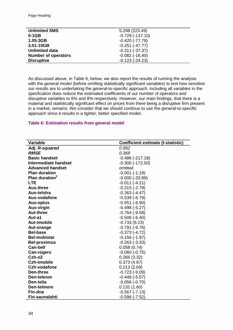
Page Heading

34

As discussed above, in Table 6, below, we also report the results of running the analysis with the general model (before omitting statistically significant variables) to test how sensitive our results are to undertaking the general-to-specific approach. Including all variables in the specfication does reduce the estimated coefficients of our number of operators and disruptive variables to 6% and 8% respectively. However, our main findings, that there is a material and statistically significant effect on prices from there being a disruptive firm present in a market, remains. We consider that we should continue to use the general-to-specific approach since it results in a tighter, better specified model.

Table 6: Estimation results from general model

Unlimited SMS 5.298 (223.49) 0-1GB -0.729 (-137.10) 1.05-3GB -0.420 (-77.79) 3.01-10GB -0.251 (-47.77) Unlimited data -0.311 (-37.37) Number of operators -0.082 (-16.40) Disruptive -0.123 (-24.23)

Variable Coefficient estimate (t-statistic)

Adj. R-squared 0.992 RMSE 0.368 Basic handset -0.486 (-217.18) Intermediate handset -0.300 (-172.50) Advanced handset omitted Plan duration -0.001 (-1.19) Plan duration2 -0.000 (-33.89) LTE -0.011 (-4.21) Aus-three -0.315 (-2.79) Aus-telstra -0.363 (-4.47) Aus-vodafone -0.539 (-6.79) Aus-optus -0.551 (-6.90) Aus-virgin -0.498 (-5.27) Aut-three -0.764 (-9.58) Aut-a1 -0.506 (-6.40) Aut-tmobile -0.733 (9.23) Aut-orange -0.791 (-9.76) Bel-base -0.373 (-4.72) Bel-mobistar -0.156 (-1.97) Bel-proximus -0.263 (-3.33) Can-bell 0.058 (0.74) Can-rogers -0.060 (-0.75) Czh-o2 0.266 (3.32) Czh-tmobile 0.373 (4.67) Czh-vodafone 0.213 (2.69) Den-three -0.723 (-9.09) Den-telenor -0.449 (-5.57) Den-telia -0.056 (-0.70) Den-telmore 0.132 (1.60) Fin-dna -0.567 (-7.13) Fin-saunalahti -0.596 (-7.52)

35

Fin-sonera -0.638 (-8.05) Fra-bouygues -0.027 (-0.34) Fra-orange 0.072 (0.91) Fra-sfr 0.053 (0.68) Ger-eplus -0.482 (-6.10) Ger-mowotel -0.387 (-4.85) Ger-o2 -0.204 (-2.58) Ger-tmobile 0.068 (0.85) Ger-telkom -0.003 (-0.04) Ger-vodafone -0.035 (-0.45) Gre-cosmote 0.455 (5.77) Gre-vodafone 0.394 (4.99) Gre-wind 0.269 (3.41) Hk-three -0.334 (-4.17) Ire-three -0.093 (-1.16) Ire-o2 -0.192 (-2.43) Ire-vodafone -0.208 (-2.41) Ita-vodafone -0.113 (-1.34) Ita-wind -0.585 (-6.88) Jap-nttdocomo -0.332 (-3.84) Mal-celcom 1.231 (14.79) Mal-maxis 0.771 (9.04) Nld-kpn 0.089 (1.13) Nld-mtv 0.312 (3.92) Nld-sizz 0.204 (2.57) Nld-tele2 0.261 (3.29) Nld-telefort 0.115 (1.45) Nld-tmobile 0.056 (0.71) Nld-vodafone 0.154 (1.95) Nor-netcom -0.429 (-5.40) Nor-tele2 -0.294 (-3.61) Nor-telenor -0.372 (-4.70) Nz-2degrees -0.162 (-2.06) Nz-telecom 0.001 (0.02) Nz-vodafone 0.224 (2.81) Pol-orange 0.080 (1.01) Pol-tmobile -0.088 (-1.10) Por-meo 0.459 (5.19) Por-optimus omitted Por-vodafone -1.059 (-9.43) Rsa-mtn 0.604 (7.15) Rsa-virgin 0.246 (2.57) Rsa-vodacom 0.631 (7.95) Spa-movistar -0.155 (-1.91) Spa-orange -0.145 (-1.84) Spa-vodafone 0.025 (0.31) Spa-yoigo -0.112 (-1.47) Swe-three -0.385 (-4.70) Swe-tele2 -0.434 (-5.46) Swe-telenor -0.442 (-5.49) Swe-telia -0.478 (-6.02) Uk-ee -0.180 (-2.26) Uk-o2 -0.099 (-1.25) Uk-orange -0.241 (-3.04) Uk-tmobile -0.286 (-3.61)

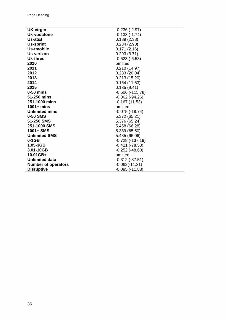
Page Heading

36

UK-virgin -0.236 (-2.97) Uk-vodafone -0.138 (-1.74) Us-at&t 0.189 (2.38) Us-sprint 0.234 (2.90) Us-tmobile 0.171 (2.16) Us-verizon 0.293 (3.71) Uk-three -0.523 (-6.53) 2010 omitted 2011 0.210 (14.97) 2012 0.283 (20.04) 2013 0.213 (15.20) 2014 0.164 (11.53) 2015 0.135 (9.41) 0-50 mins -0.506 (-115.78) 51-250 mins -0.362 (-94.26) 251-1000 mins -0.167 (11.53) 1001+ mins omitted Unlimited mins -0.075 (-18.74) 0-50 SMS 5.372 (65.21) 51-250 SMS 5.376 (65.24) 251-1000 SMS 5.458 (66.28) 1001+ SMS 5.389 (65.50) Unlimited SMS 5.435 (66.06) 0-1GB -0.728 (-137.19) 1.05-3GB -0.421 (-78.53) 3.01-10GB -0.252 (-48.60) 10.01GB+ omitted Unlimited data -0.312 (-37.51) Number of operators -0.063(-11.21) Disruptive -0.085 (-11.88)

37

Annex 4

4 Robustness testing As we discuss above, we have conducted a number of tests of the robustness of the analysis. This is important in assessing whether the results are driven by any specific factors or, instead, whether they are broadly robust. This Annex sets out in more detail the robustness tests we have undertaken.

Functional form

The Box-Cox Test

As discussed in Section 3, a key consideration with hedonic analysis is that the relationship between price and the characteristics of the product may not be linear – prices may increase at an increasing or decreasing rate when characteristics change. To test this, we estimated a Box-Cox model. This model allows one to estimate a range of models that encompass a linear model, a log-linear model and a wide range of models in between. The model allows the analyst to estimate what non-linear transformation fits the data best. In particular, the Box-Cox model includes two types of transformations:

Box-Cox transformation of price = (priceθ -1) /θ

Box-Cox transformation of independent variables = (independent variablesλ -1) /λ

Ultimately, the method reports the value of θ and λ that maximise the likelihood function. The values of θ and λ can differ. Interpretation of the model parameters includes many common cases, such as:

θ and/or λ value Transformation

1.00 Linear regression model

0.50 Square root transformation

0.33 Cube root transformation

0.25 Fourth root transformation

0.20 Fifth root transformation

0.00 Natural log transformation

Our test of the data suggests a θ = 0.193 and a λ = 1.653. There are a number of ways in which we could use this to inform our choice of model specification. Three obvious ones are:

a) Strictly use the results from the Box-Cox model

b) Ignore the test results and assume a linear relationship instead

c) Use values which are close to the Box-Cox model but are easier to conceptualise and interpret. Here we assume a θ = 0 (which is equivalent to a natural log transformation) and λ = 2 (a square transformation) 85. These values are chosen

85

There are only two variables in our model which are not dummy variables (plan duration and number of operators). We transform the plan duration variable but do not do so for the number of operators variable. This is because it is close to a dummy variable (only taking three values) and because, as we discuss in our market concentration robustness test, we consider that the number of operators variable could have been included as a dummy variable.

Page Heading

38

because they are the closest meaningful values to those indicated by the Box-Cox model

In Table 7, below, we set out the results from running the analysis using these three transformations.

Table 7: Comparing model specifications

Variable Specification a Specification b Specification c

AIC 225886.5 2257677 203878.3 No. operators -0.036 (-17.72) -5.276 (-16.77) -0.082 (-16.40) Disruptive -0.050 (-24.00) -5.276 (-15.74) -0.123 (-24.23)

Comparing these models cannot simply be done using standard tools such as the adjusted R-squared or RMSE. This is because the models have different numbers of explanatory variables and the dependent variable is transformed differently in each case. R-squared and RMSE are only useful where you are comparing like-for-like in this respect.

A more appropriate measure of fit than R-squared and RMSE in this instance is the Akaike Information Criterion (AIC) test of model selection which is included in Table 7. This test is commonly used in non-linear models which can be estimated by the method of maximum likelihood, such as this one. It is also particularly attractive for this analysis since it does not require the models to be nested (i.e. where both models are the same except one is missing some variables which are included in the other) and is best suited to large datasets.

Unlike many statistical tests, the AIC does not test using a null hypothesis which is either rejected or not. Instead, the model with the best fit is simply the one with the lowest AIC value.

The results in Table 7 indicate that we should prefer specification ‘c’ because:

a) It is closer to the form suggested by the Box-Cox model than specification ‘b’;

b) Specification ‘a’ is unhelpful because it has no clear interpretation for the purposes of our analysis.86

c) Specification ‘c’ has the lowest AIC.

Handsets

As noted above, many other studies of this nature exclude handset data because of a concern that a preference for handsets is being estimated rather than mobile tariffs.

As set out in Section 4, we consider that handsets are an important element of the mobile offering. Notwithstanding, we have carried out a robustness test on the approach we have taken to include handset data.

Table 6, below, reports the main results of our estimation when handset charges are not included.

86

We can, however, easily interpret the results of specification ‘b’. These show that the presence of a disruptive firm will reduce prices by approximately $5.23 on average. If we assume that an average tariff costs $50 per month, this translates into an effect of around 10.5% which is not too dissimilar from the 11.6% finding in specification c.

39

Table 8: Excluding handset charges

Variable Handset charges omitted Main specification

Adj. R-squared 0.987 0.992 RMSE 0.434 0.389 4 operators -0.002 (-0.33) -0.082 (-16.40) Disruptive -0.029 (-4.72) -0.123 (-24.23)

These results show a reduced effect of both the number of operators and disruptive firms on price when handset data are omitted from the model. However, the effects are still in the same direction.

To help understand whether we should prefer to include handset charges or not, we undertake an F-test to test whether the handset variables are jointly significant. Testing the null hypothesis that the handset variables are jointly insignificant yields F=27815. This is substantially larger than the critical value so indicates that we can reject the hypothesis that the handset variables are jointly insignificant.

Both this statistical test and our theory (as set out in Section 4) indicate that we should include handset charges in our analysis. In particular, we consider that excluding handset data from the analysis will bias the results. This is because we consider that each handset and tariff combination should be a unique observation since this is the real choice that consumers face when they look to purchase a new mobile and plan. The result of omitting this data is that we lose a huge number of observations and it is likely that the new sample dataset will not be representative of the population data. For example, it is often the case that monthly tariff prices change depending on which handset is chosen – the analysis with handset charges omitted will necessarily not allow for this.

Alternative methods of allowing for unlimited allowances

As we discuss in Section 4, we use categorical variables for the minutes, texts and data allowances so that we are able to include unlimited allowances in the analysis. An alternative method we could employ would be to use the actual, continuous, values of the allowances and set arbitrary large numbers for the unlimited values instead of grouping allowances together to construct categorical variables. This would have the advantage of not constraining the data to a certain number of categories but would, necessarily, involve a subjective assessment of what values should be allocated to unlimited allowances. We test this alternative method by using the continuous values of non-unlimited allowances and setting unlimited allowances as:

a) 1,000 minutes, 1,000 texts and 15GB of data

b) 5,000 minutes, 5,000 texts and 30GB of data

c) 10,000 minutes, 10,000 texts and 60GB of data

d) 20,000 minutes, 20,000 texts and 100GB of data

Page Heading

40

There is no specific reason for choosing these variables, we have simply chosen a variety of arbitrary values which are larger than the largest non-unlimited observation87. The results from doing this did not differ significantly from the approach of using categorical variables and does not change the fit of the model. We, therefore, choose to use categorical variables to avoid having to make an arbitrary judgement on the numerical value of unlimited variables.

Table 9: Continuous allowances

Variable Scenario a Scenario b Scenario c Scenario d

Adj. R-squared

0.991 0.991 0.990 0.990

RMSE 0.376 0.402 0.407 0.413 No. operators -0.112 (-21.05) -0.061 (-10.70) -0.057 (-9.94) -0.049 (-8.33) Disruptive -0.135 (-24.90) -0.137 (-22.50) -0.136 (-21.92) -0.131 (-20.73)

Tests of country-specific and year-specific factors

We tested whether the results are driven by any particular country. The way in which we do this is by systematically excluding all observations for each country from the dataset and then re-running the analysis. Doing this has little effect on the outputs and fit of the model in each case so we conclude that the results are not driven by the data for any particular country.

We also tested whether the results are driven by observations in any particular year. In a similar way to how we tested for the effects of different countries, we systematically excluded observations for each year from the dataset and re-ran the analysis. Again, doing so had little effect on the outputs of our analysis so we conclude that the results are not driven by observations in one particular year (for simplicity of presentation we do not present the results of these robustness tests here).

Tests of aspects of pricing plans

We tested whether any aspect of operators’ pricing plans materially impact the results by systematically excluding the observations associated with each category of minutes, texts and data allowance. In the same way, we also test whether the inclusion of certain handset categories, whether the plan is LTE or not and the contract length have a material effect on the results. Although, in some cases, these tests changed the magnitude of the results (although, not dramatically), they had no impact on the broad finding that, on average, the presence of a disruptive firm reduces mobile prices. We, therefore, consider that our analysis is robust with respect to these factors (again, given the number of robustness tests carried out on pricing plan aspects, we do not report the results here).

Tests of different categorisations of disruptive firms

As we discuss above, our process of identifying whether a firm is disruptive or not is necessarily subjective. We, therefore, ran a number of tests which categorise disruptive firms in different ways. There are a number of firms which we consider to be almost definitely

87

This reflects the necessary arbitrary nature of this approach. One potential option would be to define these based on observed consumption of mobile services. However, this would be difficult to do in practice given differences across countries.

41

disruptive under our classification88. We do not test the cases where these firms are not disruptive since we have confidence that they are and any analysis based on this would lack the theoretical foundations to have any real meaning. Instead, we consider cases where we have less certainty over the classification. These are:

a) Where Yoigo is never disruptive in Spain

b) Where Yoigo has always been disruptive in Spain

c) Where Optimus was not disruptive in Portugal

d) Where T-Mobile is never disruptive in the US

e) Where Three was not disruptive in the UK after 201489

Experimenting with the make-up of the disruptive dummy variable in this way has little impact on the results of the analysis and does not change the overall finding that the presence of disruptive firms significantly reduce prices in the countries in which they operate in any case. We, therefore, consider that the analysis is robust to sensible variations in the categorisation of disruptive firms.

Table 10.1: Alternative disruptive firm definitions

Variable Scenario a Scenario b Scenario c Scenario d

Adj. R-squared

0.992 0.992 0.992 0.992

RMSE 0.369 0.369 0.369 0.369 No. operators -0.088 (-16.57) -0.088 (-16.57) -0.080 (-15.42) -0.080 (-15.03) Disruptive -0.111 (18.45) -0.111 (-18.45) -0.129 (-25.12) -0.127 (-22.30)

Table 10.2: Alternative disruptive firm definitions

Variable Scenario e

Adj. R-squared

0.992

RMSE 0.369 No. operators -0.092 (-17.99) Disruptive -0.110 (-22.65)

Different concentration measure

In the main specification, we include a variable which takes the value of the number of MNOs in a national market in each year. An alternative market concentration measure would be a dummy variable which took a value of one if there are four or more operators present in the market in that year or zero if there are fewer. This would more explicitly give us an indication of the average effect of moving from a four player market to one with three. Under this approach, the finding that prices in markets with a disruptive firm are significantly below those without one remains. The fit of the two models is quite similar so we make a

88

For example, European MNOs which belong to Hutchison Group and have not merged with/acquired other MNOs in their market. 89

We do not consider it likely that Three is no longer disruptive in the UK market. However, we have included this robustness check since Three has argued this point as part of the ongoing discussions about its proposed merger with O2 in the UK.

Page Heading

42

judgement call to use the number of operators variable as we consider it to be a variable which describes the situations in national markets more fully.

Table 11: Different concentration measure

Variable Coefficient (t-statistic)

Adj. R-squared 0.992 RMSE 0.368 4 operators -0.101 (-20.42) Disruptive -0.151 (-31.13)