Econometric issues in the analysis of linkedcross-section employer-worker surveys¤

Andrew Hildrethy Stephen Pudneyz

April 1998: Preliminary - please do not quote.

Abstract

We consider the statistical problems involved in the econometric

analysis of data from linked surveys of workers and employers. The

context is a simple model of the incidence and duration of unemploye-

ment spells occurring between two waves of the UK New Earnings

Survey, which have been linked to unemployment bene¯t records via

the National Insurance number, and to Census of Production respon-

dent ¯rms via the Inter-Departmental Business Register.

JEL Classi¯cation: C1, C8, J3, J6

1 Introduction

It is only comparatively recently that economists have started to consider

seriously the role of employer behaviour in determining the employment and

¤`Econometric issues in the analysis of linked worker-employer cross-section surveys'.We are grateful to the O±ce for National Statistics for access to respondent-level data

from the New Earnings Survey and Annual Census Of Production, and for their e®orts

in implementing the linking process. All the views in this paper are our own and not

necessarily those of the ONS. This research was supported by the Economic and Social

Research Council through grant no. R000222231, and the Leverhulme Trust through the

Institute of Labour Research at the University of Essex.yDepartment of Economics and Institute for Labour Research, University of EssexzPublic Sector Economics Research Centre, Department of Economics, Leicester

University

1

remumeration of individuals, the rate of labour turnover, and worker selec-

tion. A move away from partial equilibrium models entails considering all

agents in the labour market, and consequently requires a much richer data

set for empirical research. The price to be paid for this is usually a much

more complex data set design. If we are to avoid using a small case study

approach to examine empirically equilibrium theories of the labour market,

then matched worker-employer datasets provide the only way forward. The

degree to which data are representative depends on the sampling structure,

the success of the survey in obtaining su±cient response, and the variables

available within the survey design. A natural avenue to explore in obtain-

ing representative matched data lies in the use of Government surveys and

administrative records.1

Models of the labour market provide the motivation for such work. The

recent wage determination literature on rent-sharing or insider-e®ects shows

that employer attributes can in°uence the pay received by workers (see Hil-

dreth and Oswald, 1997 as an example). Such work usually uses longitudinal

information from company accounts data bases where the dependent vari-

able is an aggregated average wage for the average employee. No individual

worker characteristics are considered. However, Abowd, Kramarz and Mar-

golis (1997) analyse the wage determination process and ¯nd that employee

characteristics make the largest contribution to the determination of observed

pay di®erences.

Combining homogenous employers and workers in two-sided search mod-

els results in models that have wage di®erentials consistent with atomistic

wage determination once the e®ects of matching frictions are recognised (Bur-

dett and Mortensen, 1997; Coles, 1997). In such models a mixed strategy

equilibrium is posited where employers post a wage and individuals search

for jobs. Matching frictions exist in the form of lags in the arrival of informa-

tion about the availability and form of job o®ers. As the matching frictions

disappear, competitive wage determination prevails, but wage di®erentials

still exist, even when workers are all equally productive. One-sided worker

or employer heterogeneity can be introduced into the model without a®ect-

ing the substantive conclusions. In particular, the equilibrium model o®ered

1Work along such lines has already been carried out in France and the USA. For

France see work by Abowd, Kramarz, and Margolis (1996), Entorf and Kramarz (1997),

and Margolis (1996). For the US, see work by Troske (1996).

2

by Coles (1997) presents a number of testable propositions concerning wage

determination, ¯rm size and performance, and movement of individuals be-

tween jobs and unemployment. In equilibrium, wages, ¯rm size and pro¯ts

are positively correlated, but are negatively correlated with the quit rate.

Small ¯rms, in equilibrium, announce low wages to extract the search rents

of their employees, and accept the higher quit rate. The observable conse-

quences of such models are clear. It should be observed that large employers

will lose few employees to other ¯rms for higher wages, su®er essentially no

quits into unemployment, have workers with a higher marginal product, and

make greater pro¯ts. Small employers will have a greater number of em-

ployees leaving, either to larger employers, or to unemployment (if the wage

o®er falls below the reservation wage level), workers with a lower marginal

product, and make lower pro¯ts. Linking workers and employers thus allows

full modelling of the labour market, relating characteristics of both sides of

the market. By including unemployment records it also becomes possible

to trace individuals between employment opportunities. With the matched

data we can examine the role of employer characterisitics on the individual

worker's wage; we can model an individual's experience of job switching and

unemployment and the type of employers that individuals either move to and

from.

However, there are statistical problems to be faced in using these matched

samples. There are three major problems here. One is the absence of cer-

tain variables that one would like to be able to use (typically individual-

and household-speci¯c variables which are relevant to individual productiv-

ity (e.g. education and training) and to individual reservation wages (e.g.

other sources of household income). There are a number of ways around

such dilemmas if Government data are to be used for analysis. One possi-

bility would be to link existing employer and worker surveys to household

surveys, which are currently completely independent. For example, in the

UK the New Earnings Survey (NES) sample of employees could in principle

be linked to respondents to the Family Expenditure Survey (FES), if Na-

tional Insurance Numbers were collected as FES data. This is impractical

for the foreseeable future, so the problem of missing variables remains an

important one.

A second potential di±culty, which is the main focus of the present paper,

is the impact of non-standard sampling properties on econometric estimation

procedures. At ¯rst glance, the use of administrative Government data would

3

appear to be ideal in this respect. Government agencies have access to very

good sampling frames and (in the UK at least) they have legal powers to

compel employers to cooperate with surveys like the NES and the Annual

Census of Production (ACOP). However, even in cases where surveys are

based on random sampling and linked to administrative records which are

in principle complete, non-response still occurs, and merging di±culties can

create a non-representative sample and inconsistency in estimated model

parameters.2

In the next section we discuss the design of each survey, describe how the

linkages between data sets are made and discuss the problems that this cre-

ates. We then consider sampling problems and their implications for models

of labour market behaviour in the context of simple cross-section, rather than

panel, estimation. In section 4, we present empirical models of wage deter-

mination, the probability of an unemployment spell in the 12 months after

NES sampling, and labour demand by employers. We show that, when using

matched data, the use of employer data in individual level equations does

not give biased estimates, despite the non-uniform sampling scheme used in

the ACOP, and we are able to establish the importance of employer-variables

such as pro¯tability and ¯rm size. However, the size-related design of ACOP

does give rise to potentially biased estimates of employment equations. Cor-

rections are made using conditional and weighted maximum likelihood ap-

proaches, but biases appear to be small. We leave for future work the much

more complex issue of the biases that may be introduced when two or more

years' data are linked to form an endogenously-sampled panel.

2 The NES-JUVOS-ACOP matched survey

The possibility of constructing this matched UK dataset comes from the de-

velopment of the IDBR (Inter-Departmental Business Register) at the O±ce

for National Statistics (ONS). The register was developed to resolve inconsis-

tencies that occurred between the maintenence of separate sampling frames

between the ONS (formerly the Central Statistical O±ce) and the Employ-

ment Department. In particular, the maintenance of the Annual Census of

Production (ACOP) by the ONS and the New Earnings Survey (NES) by

2See Hildreth (1996) and Hildreth and Pudney (1996).

4

the Employment Department was done from two seperately maintained reg-

isters of businesses in the United Kingdom. Di®erences in classi¯cation and

coverage between the two registers led to di®erent estimates of key economic

indicators, especially employment. The main administrative sources that

contribute to the IDBR are the VAT (value added tax) and PAYE (pay as

you earn) tax registers. The only sectors that are not covered are some parts

of agriculture, and some other very small businesses, for example the self-

employed and some non-pro¯t organisations. The statistical unit for both

registers is an enterprise. An enterprise can be a single entity or a group

of legal units. The IDBR has been used for sampling purposes for both the

NES and ACOP since 1994. Our work concerns the two cross-sections for

1994 and 1995.

2.1 The New Earnings Survey (NES)

The NES is an annual sample survey of earnings of employees in Great Britain

of employees in employment. The survey is based on a one percent sample

of employees who are members of the PAYE tax scheme. Questionnaires

are sent to employers to be ¯lled out on employees selected as part of the

sample. Individuals are identi¯ed by means of their national insurance num-

bers (NINO), which are randomly allocated to individuals when they attain

working age. All individuals whose NINO ends with the digits 14 are selected

as the sample. Although national insurance numbers are individual-speci¯c,

and might be deemed to be a unique identi¯er, they are not in practice. A

very small number of national insurance numbers are allocated to more than

one individual through administrative re-using of the same number. Since

1975 the same last two digits have been used with each successive wave of

the NES.

Employees are identi¯ed in the survey by one of two methods. About

90 percent of the sample is identi¯ed from lists supplied by the Inland Rev-

enue containing the selected national insurance numbers and the names and

addresses of their employers. To the employer is attached an enterprise refer-

ence number (ENTREF), taken directly from the IDBR. The remaining part

of the NES sample is obtained directly from certain large employers, mainly

in the public sector. Once again, these enterprises will carry an ENTREF.

The information collected in the NES concerns earnings for a particular

pay period (determined and reported by the employer). Other information

5

is limited to hours worked per week (basic and overtime), age, occupation,

industry, collective agreement coverage, and location. The gender of the

respondents is not actually recorded as part of the NES, but gender records

are provided by the Inland Revenue to the NES as part of the initial sample

check list. The Inland Revenue provide a new list each year. Where there is

a change in gender, or the record is missing, the record is checked against a

DSS (Department of Social Security) ¯le called `Ledger 14'. Ledger 14 gives

a complete listing of all NINO's ending in 14 together with the gender of the

individual.

2.2 The Joint Unemployment and Vacancies Operat-

ing System (JUVOS)

As the same set of national insurance numbers have been used for the NES

since 1975, the same set of individuals should normally be in the sample from

one year to the next. However, non-response by an employer about an indi-

vidual can occur for one of two principal reasons. Firstly, the individual may

no longer be part of the labour force, owing to retirement, maternity leave, or

other forms of absence. Secondly, the individual may be unemployed. If he

or she registers as being unemployed, then this is recorded against the NINO,

provided he or she claims unemployment bene¯t (or other unemployment-

releted bene¯t). These records are maintained by the Department of Trade

and Industry (DTI). The unemployment bene¯t (UB) records provide infor-

mation on a quarterly basis on whether a spell of registered unemployment

occurred and how long (in days per quarter) it lasted. The computer records

are up-dated on a monthly basis.

The UB records are taken from JUVOS (Joint Unemployment and Va-

cancies Operating System). The JUVOS dataset is a ¯ve percent sample of

all computerised claims for unemployment bene¯t, initially in the ¯rst quar-

ter of 1983, but updated continuously since then to take account of all new

claimants. The sample chosen is based on the last two digits of the NINO

with 14, 24, 44, 64, and 84 as the selected numbers. Individuals whose NINO

ends in 14 are in principle the same as those individuals included in the NES

sample. If an individual has claimed unemployment bene¯t since the com-

puterised records began, then his or her history of registered unemployment

is known. The one variable we use from the JUVOS records here is the

6

number of days within a quarter that an individual is unemployed, and this

denotes both whether an unemployment spell occurred and the proportion

of a year that an individual is unemployed.

2.3 The Annual Census of Production (ACOP)

The ACOP is not a true census, but rather a sample survey. Each year,

the ACOP samples approximately 20000 establishments (reporting units)

in the energy and utility, manufacturing, mining, and construction sectors.

Reporting units are drawn from the IDBR via the ENTREF. As such, the

enterprise unit from the IDBR is at a greater level of aggregation than the

reporting unit. For each ENTREF, there are local units that have their own

reporting reference (RUREF). The basis for sampling in the ACOP is done

using the RUREF. The RUREF is a unique identi¯er for each reporting unit.

The reporting unit is essentially the mailing address for the ACOP forms.

A separate mailing address should be given for each type of activity at the

enterprise. Information at the reporting unit level is collected on a number

of variables, including employment, turnover, value added, stocks of goods

or materials, wages and capital expenditure.

Unfortunately, the sampling structure of ACOP changed between the

years 1994 and 1995 that we analyse here, and this is the source of some

technical di±culty. In 1994, all ¯rms in the target sectors with 100 employ-

ees or more were included in the sample with probability 1. Below this size

cut-o®, establishments were sampled on a strati¯ed basis with probabilities

di®ering across size and industrial sector. In 1995, the threshold for exhaus-

tive sampling was made sector-dependent, and raised to 200 employees for

many sectors. The main e®ect of size strati¯cation below the cut-o® is to

exclude very small ¯rms. In particular, the ACOP samples contain virtually

no reporting units with fewer than 10 employees.

2.4 Linking workers and employers

Linking individual records between NES and JUVOS is straightforward. Se-

lecting only those individuals from JUVOS whose NINO ended in 14, the

match is then simply obtained using the NINO as a key. Where individuals

do not have an unemployment record, the number of days spent unemployed

in any quarter of the year is assumed to be zero.

7

Although in principle it should be possible to create a known unique

match from individual to establishment, linking across the NES and ACOP

data sets is much more problematic. Firstly, the link between individual

and establishment has to be made via the ENTREF, which refers to a whole

enterprise, and is not unique for any individual/establishment pair. To create

the unique match it has to be inferred from the IDBR records. As a reporting

unit is supposed to be, by de¯nition, an activity at a particular address, the

combination of an enterprise reference and industrial sector, given by the

¯ve digit 1992 Standard Industrial Classi¯cation (SIC) code, should provide

a unique identi¯cation of an establishment. This same identi¯cation is then

available on each individual in the NES, provided we make the assumption

that the SIC code as recorded in the NES and ACOP are the same. However,

the allocation of establishments to SIC sectors is not always unambiguous,

so there is scope here for matching failures.

In creating the match across the NES and ACOP a number of observations

were lost from multiple entries for individuals by national insurance number,

and from cases where the ENTREF and SIC code did not create a unique

identi¯cation. Table 1 summarises the information loss from matching in

this way. Information from non-unique national insurance numbers in each

wave contributes to only a 1-2 percent loss of information. In the 1994 NES,

a greater amount of information is lost from the ENTREF being missing

for a number of NES respondents. The missing ENTREF was the result

of some organisations (public authorities and national corporations) being

contacted directly because of their prominence in the labour market, rather

than through the IDBR. The 1995 NES does not su®er from this missing

information problem. Without the ENTREF, no link can be made between

NES respondents and ACOP establishments.

8

Table 1a: Observation Loss from the NES by National Insurance

number (NINO).

Source 1994 1995

Sample issued 209900 213500

Response 166634 162068

Observations lost from repeat NINO 4021 2112

Observations available for matching to JUVOS 162613 159955

Observations lost from missing ENTREF 27309 1982

Observations remaining for match to ACOP 135304 157974

Table 1b: Observation Loss from the ACOP by Reporting Unit

reference number (RUREF).

Source 1994 1995

ACOP sample issued: total 16035 15458

Sample issued: <100 employees 8496 9140

Sample issued: 100+ employees 7539 6318

Response: total 12684 12051

Response: <100 employees 6368 6638

Response: 100+ employees 6316 5413

Number of enterprises matched to NES 3861 3591

Number of establishments matched to NES 4438 4052

< 100 employees 1140 1021

100+ employees 3298 3031

NES subjects in matched establishments 14548 15664

Once the NES and ACOP are matched, it gives individuals at establish-

ments where we knew that the match is unique. There are however a few

sampling anaomalies in this match because of di®erences in survey dates,

since the NES is carried out in the ¯rst quarter of the year, while the ACOP

draws the sample from the IDBR and carries out the survey in the ¯nal

quarter of the year. The ¯nal two rows of Table 1b show that about 66 er

ce t o es ab is me ts n t e A OP espondents could be matched to NES

respondents. In approximately 30 percent of the cases there was more than

one sampled worker per establishment.

9

Figures 1 and 2 illustrate the distribution of ¯rm size in terms of work-

ers per establishment for 1994 and 1995. They compare the distribution of

¯rm sizes as recorded on IDBR with the distribution in the achieved ACOP

sample and the NES-matched ACOP subsample. They show very clearly

the enormous impact of di®erential sampling rates and the consequent scope

for bias introduced by sampling distortions. The number of workers per es-

tablishment in the actual population has a distribution that is fairly close to

exponential form, while the sample distribution is very strongly skewed in the

opposite direction, and much closer to lognormal form. The major change in

the ACOP sampling scheme between 1994 and 1995 is also evident.

A striking feature of table 1 and ¯gures 1-2 is the way that the sample

becomes still more skewed towards large establishments when we restrict

selection to establishments containing at least one NES subject. It may

be useful to do this, since some variables (such as location) are available

from NES and not from ACOP. Also one might want to use the personal

characteristics of NES subjects to construct summary measures of the ¯rm's

workforce. The problem with this is that large establishments are more

likely to yield a NES subject, and thus large establishments dominate the

matched sample.This type of sample distortion may be very important for

some analytical purposes, and we return to this issue below.

3 A model of the sampling / linking process

3.1 The cross-section sample distribution

De¯ne the following notation, relating to a single survey year. We have three

sources of information:

(i) NES information on individuals who are in employment, denoted w;(ii) JUVOS information on individuals' current and past experience of

unemployment, denoted u;(iii) ACOP information on the characteristics of the employer, denoted

(f; S), where S is ¯rm size measured by employment and f is a vectorcontaining all other ¯rm characteristics.

Our task is now to derive the sample distribution of the observations from

a single year's data on employees and their employers, to provide a basis for

10

Figure 1: Size distributions for establishments in IDBR population and full

sample and NES-linked subsample of ACOP for 1994

11

Figure 2: Size distributions for establishments in IDBR population and full

sample and NES-linked subsample of ACOP for 1995

12

drawing inferences about the processes of pay determination, job loss and

unemployment. From the viewpoint of the theoretical statistician, there is

a serious problem to be overcome in analysing the dataset that results from

the ¯rm-worker matching process described in section 2. The techniques

customarily used to model survey data are based on the assumption of an

underlying continuous distribution. For example, probit or Tobit analysis

requires that behavioural disturbances are drawings from a normal distrib-

ution; logit analysis is based on the logistic distribution. But a distribution

can only be continuous if the population it describes is in¯nite. Since the

total number of ¯rms and workers in existence at any time is very large, one

usually feels safe in using these in¯nite-population methods for analysing

company or worker cross-sections. However, with matched data, this is more

problematic. If there are in¯nite numbers of ¯rms and workers, then the

probability of observing even a single ¯rm-worker match is essentially zero

in any ¯nite sample, unless there exist ¯rms of in¯nite size. There is a fur-

ther problem in the case of the ACOP, since the survey design requires that

every ¯rm in the target production sectors is sampled with probability 1 if

its workforce exceeds a pre-speci¯ed threshold size. In an in¯nite population

of ¯rms, this would generally imply an in¯nite sample of large ¯rms.

Fortunately, a suitable theoretical framework is available for situations

like this. Superpopulation theory (Cassel et. al., 1977; Pudney, 1989) al-

lows us to work with a ¯nite population, by postulating the existence of an

underlying in¯nite superpopulation from which the actual ¯nite population

is assumed to have been drawn at random by \nature". Essentially, the su-

perpopulation describes the set of possible forms the actual ¯nite population

might have taken. The objective of our statistical analysis is then to estimate

fundamental relationships present in the superpopulation - in other words the

(random) processes that govern the nature of the actual population we see

around us. Since the superpopulation is in¯nite, it is admissible to estimate

these statistical relationships using techniques which assume continuous dis-

tributions. However, in doing so, it is necessary to take proper account of

the fact that the process generating our data has two stages - a draw (made

by \nature") from the superpopulation, followed by a second draw (made by

the survey designer) from the ¯nite population.

At any particular time, the superpopulation consists of an in¯nite set of

elements, each corresponding to a manufacturing ¯rm and its workforce. The

size of the ¯rm's workforce is s, and the information set describing the ¯rm

13

and its S workers is denoted X = fS; f; w1:::wsg 3 I the up rp pu at on

th di tr bu io of he e ¯ m/ or fo ce lu te s i de cr be by pr ba il ty

en it /m ss unct on ( df g( ). ur am le fal s i to se of st at .

E ch tr tu r i de ne by si e r nge Cr fr m w ic th su ve sa ples

at a rate ½r. F r the top stratum, an exh us iv s mp e i ta en, implying

½R = 1. For the sake of simplicity, we assume that sampling within the lowerstrata is random. The total sample size is n and the number f bservations

fr m each stratum is nr = [½rn] where [.] denotes the nearest integer. No ethat nr is random with respect to the super-population. Henceforth, we use

the symbol g( : ) as generic notation for any distribution that describes thesuperpopulation; the symbol h( : ) is used to represent sample distributions.

Largest ¯rms

Let the size of the actual population be N ¯rms, and let PR = Pr(S 2CR) = 1 ¡ GS(CR) be the frequency of large ¯rms in the superpo

n the

superpopul

R) =

ÃnRN

!P nR(1¡ P )N¡nR

n¤Yj=1

g(XjjSj ¸ CR) (1)

However, in general the collection of variables X is not fully observable,

since the NES is a 1 in (approximately) 100 random sample of NI numbers.

Thus, any particular worker has a known probability ¸ ¼ 0:01 of beingobserved in the NES. Conditional on the size of the ¯rm, S, the number ofworkers captured by the NES (q) therefore has a binomial (S; ¸) distribution.Letting the symbol fX denote the part of X that is observed, the joint sample

distribution for large ¯rms is therefore:

3For the purposes of cross-section analysis, the unemployment information u can betreated in exactly the same way as the NES information w; so there is no loss of generalityif we omit u for the sake of notational simplicity.

14

h(nR; fX1:::fXnR) =

ÃnRN

!P nRR (1¡ PR)N¡nR

£nRYj=1

g(fj; SjjSj ¸ CR)

ÃqjSj

!¸qj (1¡ ¸)Sj¡qj

qjYi=1

g(wijjfj ; Sj)

=

ÃnRN

!(1¡ PR)N¡nR

£nRYj=1

g(fj; Sj)

ÃqjSj

!¸qj (1¡ ¸)Sj¡qj

qjYi=1

g(wijjfj ; Sj) (2)

where we have used the relationship g(f; SjS ¸ CR) = g(f; S)=PRSmaller ¯rms

The remainder of the sample is a set of strata samples of smaller ¯rms.

Consider the rth stratum de¯ned as the size class Cr = (Cr; Cr). Under thesuperpopulation approach, observations on ¯rms in this stratum are viewed

as being generated as a random sample (without replacement) drawn from

a random sample drawn from the relevant part of an underlying in¯nite

population. But a random sample of a random sample is itself a random

sample, so the joint distribution of information relating to sampled small

¯rms in stratum r is the binomial probability of the stratum size Nr inthe actual population, multiplied by the joint distribution of the sample

observations conditional on the implied sample size:

h(nr; X1:::Xnr) =

ÃNrN

!(1¡ Pr)N¡NrPNr¡nrr

£nRYj=1

g(fj; Sj)

ÃqjSj

!¸qj (1¡ ¸)Sj¡qj

qjYi=1

g(wij jfj ; Sj)

(3)

All ¯rms

Thus, putting together the full sample:

15

h(N1:::NR; fX1:::fXn) =RYr=1

ÃNrN

!(1¡ Pr)N¡NrPNr¡nrr

£nYj=1

g(fj; Sj)

ÃqjSj

!¸qj (1¡ ¸)Sj¡qj

qjYi=1

g(wijjfj ; Sj)

(4)

Note that Nr ¡ nr is identically zero for r = R.

4 Cross-section estimation

We now consider the implications of the sample distribution (4) for some

simple estimation purposes.

4.1 Estimating a cross-section earnings equation

For some practical purposes, we may be interested in the distribution of

one or more worker variables conditional on the characteristics of the ¯rm

and remaining characteristics of the worker. This is so, for example, if we

use the data to estimate an earnings regression. To ¯nd this conditional

distribution, we divide the worker variables w into an endogenous variablew¤ (earnings) and the remaining conditioning variables w¤¤ (age, gender,unemployment history, etc.). We then need to integrate out the endogenous

worker variable w¤ to derive the marginal distribution of the conditioningvariables ff; s; w¤¤; q; n¤g, and then divide the full sample distribution bythis marginal. When this is done, many terms in the sample distribution (4)

cancel, and the result is the following conditional sample distribution:

h(w¤jf; s; q; n¤; w¤¤) =nYj=1

qjYi=1

g(wijjfj; sj)g(w¤¤ij jfj ; sj)

=nYj=1

qjYi=1

g(w¤ij jfj; sj; w¤¤ij ) (5)

The important result here is that this is essentially identical to the distribu-

tion of w¤ conditional on ff; s; w¤¤g in the superpopulation. Thus, the usual

16

type of sample analysis of earnings conditional on ¯rm and worker charac-

teristics will give valid inferences about the underlying (super)population.

Tables 2 and 3 give the results of estimating semi-log wage equations

separately for 1994 and 1995 for males and females, using a conventional set of

explanatory covariates from the NES and JUVOS datasets, supplemented by

ACOP ¯rm characteristics. The basic estimating equation which corresponds

to the sample likelihood above is

lnw¤ij = w¤¤ij ¯ + fj° + "

ij

where w¤ij is the wage for individual i at ¯rm j, j = 1:::n and i = 1:::qj; w¤¤ij is

a vector of individual characteristics from the NES and JUVOS datasets; fjis a vector of establishment characterisitics from the ACOP; "ij is the randomerror term.4 The earnings equation is standard apart from the inclusion of

the employer variables and the before- and after-unemployment probabilities.

The results from Tables 2 and 3 provide results consistent with others in

the literature. The age-earnings pro¯le is unusual as third and fourth power

terms are signi¯cant for men and women (although only for 1994 for women).

Coverage by a collective bargaining agreement has a positive and signi¯cant

e®ect for men, but an insigni¯cant e®ect (at normal levels) for women. All

two digit occupation and industry dummy variables are signi¯cant, as are

the 17 location dummies.

The unemployment variables show a varied pattern across time and across

gender. Unemployment incidence in the 12 months before the NES date

has a negative e®ect for men in 1994, as does the proportion of the year

spent in unemployment. For women, these e®ects are also negative, but not

signi¯cant.

Three employer variables were included in the wage equations: the log

number of employees, pro¯t per employee, and capital expenditure per em-

ployee. All coe±cients are positive, well determined (apart from capital

expenditure per employee for females in 1995), and show that the employ-

er's economic characteristics have signi¯cant e®ects on an individual's wage.

Separate equations with only one employer term were also estimated. The

4Given that there are approximately 50 percent of the observations in either cross-

section that have employers where more than 1 individual is observed at that establish-

ment, it would be possible to recover an estimate of employer ¯xed e®ects. Hildreth (1996)

provides an example of such an estimation. Such an exercise is not undertaken here.

17

result showed that the sign, size, and signi¯cance of the employer terms did

not change substantially, nor did the coe±cients on the individual-speci¯c

components. Employer e®ects on the wage appear to be important and in-

dependent of, and supplemental to, individual characteristics.

18

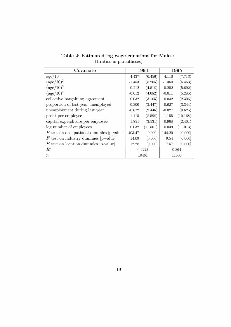
Table 2: Estimated log wage equations for Males:

(t-ratios in parentheses)

Covariate 1994 1995

age/10 4.437 (6.456) 4.110 (7.713)

(age/10)2 -1.453 (5.265) -1.360 (6.453)

(age/10)3 0.212 (4.518) 0.202 (5.692)

(age/10)4 -0.012 (4.082) -0.011 (5.285)

collective bargaining agreement 0.032 (3.105) 0.032 (2.306)

proportion of last year unemployed -0.300 (3.447) -0.627 (3.344)

unemployment during last year -0.072 (2.446) -0.027 (0.625)

pro¯t per employee 1.115 (8.598) 1.155 (10.168)

capital expenditure per employee 1.851 (3.531) 0.968 (2.401)

log number of employees 0.032 (11.501) 0.039 (11.013)

F test on occupational dummies [p-value] 403.47 [0.000] 144.20 [0.000]

F test on industry dummies [p-value] 14.09 [0.000] 9.54 [0.000]

F test on location dummies [p-value] 12.28 [0.000] 7.57 [0.000]

R2 0.4223 0.364

n 10461 11505

19

Table 3: Estimated log wage equations for Females:

(t-ratios in parentheses)

Covariate 1994 1995

age/10 1.589 (2.022) 0.954 (1.430)

(age/10)2 -0.568 (1.842) -0.282 (1.120)

(age/10)3 0.095 (1.834) 0.040 (0.979)

(age/10)4 -0.006 (1.978) -0.002 (0.992)

collective bargaining agreement 0.017 (0.681) 0.081 (2.569)

proportion of last year unemployed -0.288 (0.976) -0.448 (2.441)

unemployment during last year -0.024 (0.327) -0.068 (1.087)

pro¯t per employee 1.927 (6.487) 2.273 (7.277)

capital expenditure per employee 2.281 (2.064) 0.181 (0.227)

log number of employees 0.050 (7.434) 0.042 (5.708)

F test on occupational dummies [p-value] 45.12 [0.000] 38.15 [0.000]

F test on industry dummies [p-value] 6.11 [0.000] 4.77 [0.000]

F test on location dummies [p-value] 6.18 [0.000] 5.35 [0.000]

R2 0.350 0.300

n 3957 4023

4.2 Estimating the probability of a transition to un-

employment

The JUVOS dataset gives details of any spells of registered unemployment in

the period surrounding the NES/ACOP surveys. This allows us to estimate

a model of the probability of a separation from the ¯rm with a period of

unemployment. Since JUVOS information is available in principle for each

of our NES subjects, this entails no further sampling complications. We use

here a simple probit model of the probability that there is at least one spell of

registered unemployment in the year following the NES (speci¯cally 1994q3-

1995q2 and 1995q3-1996q2 for the 1994 and 1995 samples respectively). In

each case we use the base year's ACOP as the source for our ¯rm-speci¯c

data, thus avoiding the need to link successive years'ACOP samples.

The estimating equation was a simple probit where the dependent variable

is 1 if an unemployment spell occurs, and 0 otherwise. The same individual

and establishment characterisitics were included in the probits as in the wage

20

equation. The coe±cients in Tables 4 and 5 are the marginal e®ects evaluated

at the point of means, so that they can be read directly as the e®ect of a

unit change in the variable of interest on the probability of an unemployment

spell occurring.5

Tables 4 and 5 show that for men, the wage earned and a previous history

of unemployment have a signi¯cant e®ect on the probability of being unem-

ployed in the year following inclusion in the NES. The higher the weekly

wage, the less likely a male worker is to experience unemployment. The

existence and duration of a previous spell has a positive e®ect. In general,

no workplace variables were signi¯cant, although the industry dummies were

signi¯cant, indicating that there are important sectoral di®erences in the

probability of job loss. For 1995, capital expenditure per employee by an

employer has a negative and well determined e®ect on the probability that

a male worker will be unemployed in the succeeding year. Although capital

expenditure is not necessarily tied to technology, this result does not seem

consistent with the idea of large scale technological unemployment.

The pattern of coe±cients for females indicates that only the incidence of

unemployment in the previous year has a signi¯cant and positive e®ect on the

probability of a succeeding unemployment spell. Unionisation (i.e. collective

bargaining) helps female workers retain employment, and employer size has

a negative e®ect on the probability of unemployment.

5In other words, if the probit model is de¯ned as Pr[y 6= 0jX] = ©(X¯) then thechange in the probability for a given change in one element in X is: @©

@X= Á(X¯)¯. Finite

di®erences are used instead for dummy covariates.

21

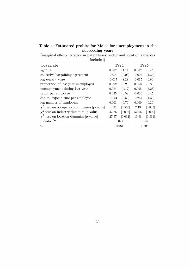
Table 4: Estimated probits for Males for unemployment in the

succeeding year:

(marginal e®ects; t-ratios in parentheses; sector and location variables

included)

Covariate 1994 1995

age/10 0.002 (1.14) 0.002 (0.45)

collective bargaining agreement -0.000 (0.03) -0.005 (1.35)

log weekly wage -0.037 (8.28) -0.015 (6.60)

proportion of last year unemployed 0.092 (3.23) 0.063 (3.89)

unemployment during last year 0.084 (5.12) 0.095 (7.23)

pro¯t per employee 0.035 (0.52) -0.020 (0.45)

capital expenditure per employee -0.124 (0.58) -0.267 (1.38)

log number of employees 0.001 (0.79) 0.000 (0.26)

Â2 test on occupational dummies [p-value] 14.21 [0.510] 7.19 [0.845]

Â2 test on industry dummies [p-value] 47.76 [0.002] 52.66 [0.000]

Â2 test on location dummies [p-value] 27.97 [0.032] 10.98 [0.811]

pseudo R2 0.091 0.148

n 10461 11505

22

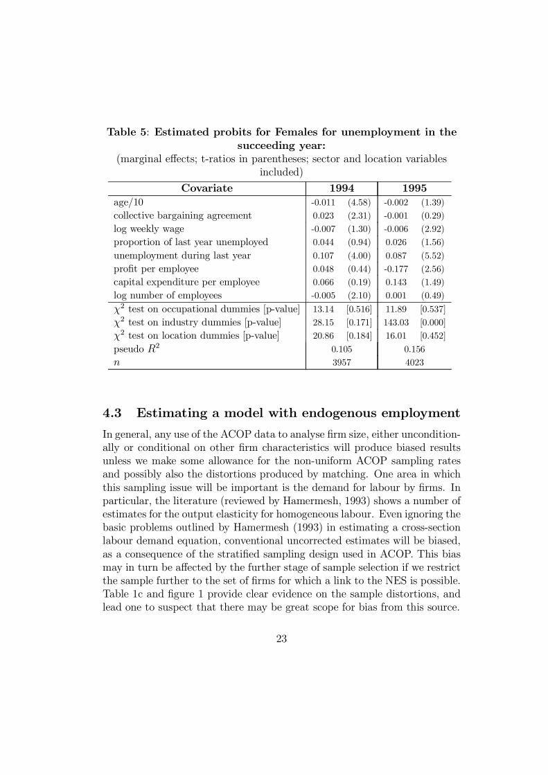
Table 5: Estimated probits for Females for unemployment in the

succeeding year:

(marginal e®ects; t-ratios in parentheses; sector and location variables

included)

Covariate 1994 1995

age/10 -0.011 (4.58) -0.002 (1.39)

collective bargaining agreement 0.023 (2.31) -0.001 (0.29)

log weekly wage -0.007 (1.30) -0.006 (2.92)

proportion of last year unemployed 0.044 (0.94) 0.026 (1.56)

unemployment during last year 0.107 (4.00) 0.087 (5.52)

pro¯t per employee 0.048 (0.44) -0.177 (2.56)

capital expenditure per employee 0.066 (0.19) 0.143 (1.49)

log number of employees -0.005 (2.10) 0.001 (0.49)

Â2 test on occupational dummies [p-value] 13.14 [0.516] 11.89 [0.537]

Â2 test on industry dummies [p-value] 28.15 [0.171] 143.03 [0.000]

Â2 test on location dummies [p-value] 20.86 [0.184] 16.01 [0.452]

pseudo R2 0.105 0.156

n 3957 4023

4.3 Estimating a model with endogenous employment

In general, any use of the ACOP data to analyse ¯rm size, either uncondition-

ally or conditional on other ¯rm characteristics will produce biased results

unless we make some allowance for the non-uniform ACOP sampling rates

and possibly also the distortions produced by matching. One area in which

this sampling issue will be important is the demand for labour by ¯rms. In

particular, the literature (reviewed by Hamermesh, 1993) shows a number of

estimates for the output elasticity for homogeneous labour. Even ignoring the

basic problems outlined by Hamermesh (1993) in estimating a cross-section

labour demand equation, conventional uncorrected estimates will be biased,

as a consequence of the strati¯ed sampling design used in ACOP. This bias

may in turn be a®ected by the further stage of sample selection if we restrict

the sample further to the set of ¯rms for which a link to the NES is possible.

Table 1c and ¯gure 1 provide clear evidence on the sample distortions, and

lead one to suspect that there may be great scope for bias from this source.

23

Using the full ACOP sample, the distribution of Sj conditional on other¯rm attributes fj is:

h(S1:::Snjf1:::fn;N1:::NR) =nYj=1

g(Sj jfj)RYr=1

hGSjf(Crjfj)¡GSjf (Crjfj)

i¡»jr

6=nYj=1

g(Sj jfj) (6)

where »jr = 1 if Sj 2 Cr and »jr = 0 otherwise. Thus, conventional uncor-rected sample-based models of ¯rm size would in general give biased infer-

ences about the (super)population distribution g(Sj jfj), and bias-correctedmethods such as weighted ML or conditional ML based on (6) are appropri-

ate.

However, if we use the ACOP subsample which contains at least one NES

match, a more complex distribution results, since we must condition also on

the event that there is a positive number of NES subjects supplied by the

establishment (qj > 0). The conditional probability of this latter event is

1¡ (1¡ ¸)Sj , so the matched-sample distribution is:

h(S1:::Snjf1:::fn; q1 > 0:::qn > 0) =nYj=1

g(Sjjfj)h1¡ (1¡ ¸)Sj

i

£RYr=1

264 CrZCr

g(Sjfj)h1¡ (1¡ ¸)S

idS

375¡»jr

(7)

In general, evaluation of this as a likelihood function would require numer-

ical integration. The use of weighted maximum likelihood is simpler, but

does not o®er a consistent estimator in this case, because reweighting the

log-likelihood function between size classes does not correct the size-related

distortion within classes, caused by the factor 1 ¡ (1 ¡ ¸)Sj . Nevertheless,reweighting is likely to ameliorate the e®ects of sample distortion to some

extent, and we now explore its use.

The cross-section labour demand model used here is intended as a vehicle

for our analysis of the impact of sampling bias, rather than as a proper

structural model. Nevertheless, similar regression models have appeared in

24

the published literature. The basic form includes a fourth-order polynomial

in the log of value-added as the output measure, together with the log average

annual wage and 23 sectoral and 17 location dummies. We have estimated

this relationship in two alternative ways: multiple regression (OLS); and

weighted maximum likelihood (WML). For the 1994 ACOP sample, the latter

is computed by maximising the following weighted log-likelihood function:

LW =nXj=1

$j ln

"g(lnSj jfj)

1¡GSjf (10jfj)#

(8)

where $j is a weighting factor equal to the known population frequency ofthe size/sector group to which ¯rm j belongs, divided by the correspondingsample frequency. The denominator of the ratio in (8) is included to re°ect

the fact that ¯rms with under 10 employees are excluded from the ACOP

sampling process. For the 1995 sample, the whole size range is sampled, so

the denominator in (8) is excluded.

Conventional estimation approaches are based on a lognormal speci¯ca-

tion for the conditional employment distribution g(Sjjfj), implying a loglin-ear population regression, with normally distributed disturbances. However,

¯gure 1 suggests very strongly that the true ¯rm size distribution is closer to

the exponential form. As a step towards improving the speci¯cation, we also

estimate a model using the Burr distribution, which nests within it the expo-

nential and Weibull distributions, and which, like the lognormal speci¯cation,

entails a linear population regression of log employment on the expanatory

variables. The Burr model is as follows:

g(lnSjf) = ¹(f)®S®

[1 + ¾2¹(f)S®](1+¾2)=¾2

(9)

where:

¹(f) = exp [¡®f¯]and the linear form f¯ is the regression function E(lnSjf). The Weibull formcorresponds to the special case ¾2 = 0 and the exponential form is generatedif we make the further restriction ® = 1. The Burr model is estimated by

WML, through the maximisation of (8), with (9) substituted for g(lnSjf).Tables 8 and 9 summarise the wage and output responses implied by the

estimated models. Four powers of log output proved signi¯cant, and thus

25

the output elasticity is not constant; we present estimates of the elasticity

evaluated at multiples 0.25, 1.0 and 2.0 of the sample average output level.

No higher-order terms, or interactions with output, were signi¯cant for the

log average wage, so the wage elasticity is simply the estimated coe±cient.

The three estimators are applied to three datasets: the linked ACOP/NES

sample, with location dummies included as explanatory variables; the full

ACOP sample (for which location is not observable); and the intermediate

case of the linked sample with location e®ects excluded. Separate estimates

are computed for 1994 and 1995.

Despite the sampling-induced biases that exist in theory, the di®erences

between the alternative estimates are not large in general. Relative to the

weighted ML estimates of either the lognormal or Burr model, OLS output

and wage elasticities di®er by no more than 0.1 or so. The Burr and lognormal

estimates show no major di®erences. Perhaps the most striking feature of

the results is the di®erence between the 1994 and 1995 estimates, which casts

doubt on the structural stability of the model

26

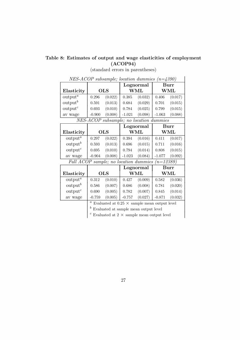
Table 8: Estimates of output and wage elasticities of employment

(ACOP94)

(standard errors in parentheses)

NES-ACOP subsample; location dummies (n=4390)

Lognormal Burr

Elasticity OLS WML WML

outputa 0.296 (0.022) 0.385 (0.032) 0.406 (0.017)

outputb 0.591 (0.013) 0.684 (0.029) 0.701 (0.015)

outputc 0.693 (0.010) 0.784 (0.025) 0.799 (0.015)

av wage -0.900 (0.008) -1.021 (0.098) -1.063 (0.088)

NES-ACOP subsample; no location dummies

Lognormal Burr

Elasticity OLS WML WML

outputa 0.297 (0.022) 0.394 (0.016) 0.411 (0.017)

outputb 0.593 (0.013) 0.696 (0.015) 0.711 (0.016)

outputc 0.695 (0.010) 0.794 (0.014) 0.808 (0.015)

av wage -0.904 (0.008) -1.023 (0.084) -1.077 (0.092)

Full ACOP sample; no location dummies (n=12389)

Lognormal Burr

Elasticity OLS WML WML

outputa 0.312 (0.010) 0.427 (0.009) 0.582 (0.036)

outputb 0.586 (0.007) 0.686 (0.008) 0.781 (0.020)

outputc 0.690 (0.005) 0.782 (0.007) 0.845 (0.014)

av wage -0.759 (0.005) -0.757 (0.027) -0.871 (0.032)a Evaluated at 0.25 £ sample mean output levelb Evaluated at sample mean output levelc Evaluated at 2 £ sample mean output level

27

Table 9: Estimates of output and wage elasticities of employment

(ACOP95)

(standard errors in parentheses)

NES-ACOP subsample; location dummies (n=3960)

Lognormal Burr

Elasticity OLS WML WML

outputa 0.449 (0.032) 0.594 (0.078) 0.775 (0.017)

outputb 0.754 (0.014) 0.825 (0.027) 0.816 (0.014)

outputc 0.824 (0.012) 0.865 (0.025) 0.836 (0.013)

av wage -0.849 (0.009) -0.523 (0.090) -0.579 (0.051)

NES-ACOP subsample; no location dummies

Lognormal Burr

Elasticity OLS WML WML

outputa 0.447 (0.022) 0.577 (0.088) 0.737 (0.084)

outputb 0.754 (0.013) 0.843 (0.028) 0.849 (0.032)

outputc 0.824 (0.010) 0.884 (0.027) 0.871 (0.035)

av wage -0.854 (0.008) -0.480 (0.105) -0.537 (0.076)

Full ACOP sample; no location dummies (n=11199)

Lognormal Burr

Elasticity OLS WML WML

outputa 0.313 (0.011) 0.231 (0.023) 0.241 (0.007)

outputb 0.612 (0.008) 0.514 (0.009) 0.535 (0.006)

outputc 0.719 (0.006) 0.647 (0.006) 0.673 (0.005)

av wage -0.758 (0.006) -0.584 (0.028) -0.612 (0.023)a Evaluated at 0.25 £ sample mean output levelb Evaluated at sample mean output levelc Evaluated at 2 £ sample mean output level

We next compare the sample ¯t of these four estimates. To do so, de¯ne

the size class indicator yj = r i® Sj 2 Cr. The conditional sample distributionof yjf is h(yjf), and this can be used to make a consistent prediction of thesample frequency of size class y as follows:

bh(y) = 1

n

nXj=1

h(yjjfj) (10)

28

However, the sample distribution h(yjf) can be written as follows:

h(yjf ) = h(y; f)=h(f)

= g(f jy)h(y)=h(f )=

g(f jy)h(y)PRr=1 g(f jy = r)h(y = r)

(11)

where h(y) is the sample frequency of size class y, determined as part of thesurvey design. The fact that the sample distribution h(f jy) can be writtenas the corresponding population distribution g(f jy) is an implication of therandom sampling that is used within size classes. But g(f jy) can be writtenas g(yjf )g(f)=g(y), and substitution of this in (11) and then (10) gives:

bh(y) = 1

n

nXj=1

g(yjfj)h(y)=g(y)hPRy=1 g(yjfj)h(y)=g(y)

i (12)

The term g(yjfj) in (12) can be computed from our estimated model, and thesampling rates h(y)=g(y) are known. Thus the predicted frequency (12) canbe evaluated and compared with actual sample frequencies as an indication

of goodness-of-¯t. The results are given in table 10.

Table 10: Goodness of ¯t for alternative labour demand models

(full ACOP samples, WML estimator)

29

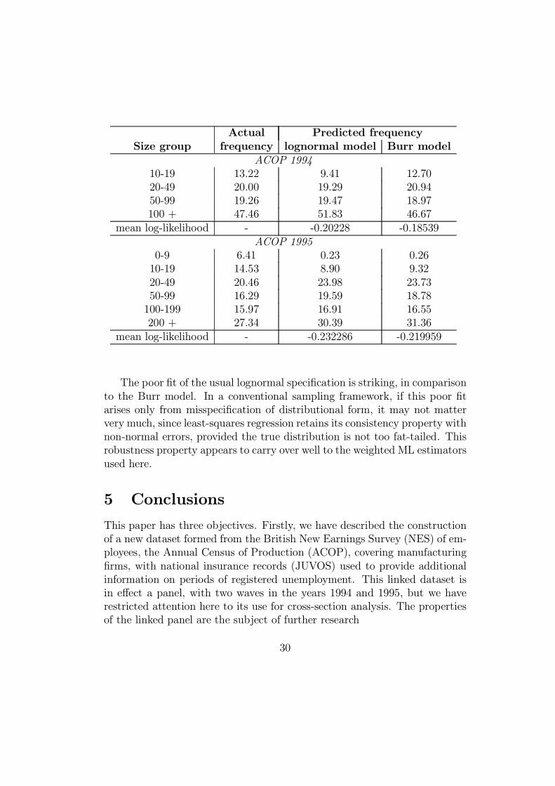
Actual Predicted frequency

Size group frequency lognormal model Burr model

ACOP 1994

10-19 13.22 9.41 12.70

20-49 20.00 19.29 20.94

50-99 19.26 19.47 18.97

100 + 47.46 51.83 46.67

mean log-likelihood - -0.20228 -0.18539

ACOP 1995

0-9 6.41 0.23 0.26

10-19 14.53 8.90 9.32

20-49 20.46 23.98 23.73

50-99 16.29 19.59 18.78

100-199 15.97 16.91 16.55

200 + 27.34 30.39 31.36

mean log-likelihood - -0.232286 -0.219959

The poor ¯t of the usual lognormal speci¯cation is striking, in comparison

to the Burr model. In a conventional sampling framework, if this poor ¯t

arises only from misspeci¯cation of distributional form, it may not matter

very much, since least-squares regression retains its consistency property with

non-normal errors, provided the true distribution is not too fat-tailed. This

robustness property appears to carry over well to the weighted ML estimators

used here.

5 Conclusions

This paper has three objectives. Firstly, we have described the construction

of a new dataset formed from the British New Earnings Survey (NES) of em-

ployees, the Annual Census of Production (ACOP), covering manufacturing

¯rms, with national insurance records (JUVOS) used to provide additional

information on periods of registered unemployment. This linked dataset is

in e®ect a panel, with two waves in the years 1994 and 1995, but we have

restricted attention here to its use for cross-section analysis. The properties

of the linked panel are the subject of further research

30

Secondly, using a theoretical foundation in superpopulation sampling the-

ory, we have considered the methodological problems raised by the linking

process and the non-uniform sampling design of the ACOP. We have estab-

lished that, for the purpose of estimating a cross-section relationship such as

an earnings equation relating the level of pay to ¯rm and worker characteris-

tics, conventional methods such as multiple regression should not be biased

by the NES/ACOP sampling scheme, provided the estimated relationship

is interpreted as holding only for jobs in the industrial sectors covered by

ACOP. However, any model with ¯rm size (employment) as an endogenous

variable will in general be a®ected by sample selection bias as a result of the

non-uniform ACOP sampling rate.

Thirdly, we have presented some estimation results for simple models

of earnings, job separations and employment. In the ¯rst two cases, these

demonstrate the importance of including in the analysis variables that can

typically only be supplied by this sort of linked dataset. Preliminary esti-

mates of the employment model suggest that, although serious bias can result

from ignoring the employment-related nature of the ACOP sampling scheme,

the actual impact may be of minor practical importance.

References

[1] Cahuc, P. and Kramarz, F. (1997) Voice and loyalty as a delegation of

authority: a model and a test on matched worker-¯rm panels, Journal of

Labor Economics, 15.

[2] Cassel, C., SÄarndal, C. E. and Wretman, J. H. (1977). Foundations of

Inference in Survey Sampling. New York: Wiley.

[3] Gregory, M. and Jukes, R. (1997). The e®ects of unemployment on sub-

sequent earnings: a study of British men 1984-94, mimeo.

[4] Hamermesh, D. S. (1993). Labor Demand. Princeton: Princeton Univer-

sity Press.

[5] Hildreth, A. K. G. (1996) Rent-Sharing and Wages: Product Demand

or Technology Driven Premia? Paper given at the STEP Conference,

National Academy of Sciences, Washington, 1995.

31

[6] Hildreth, A. K. G. and Pudney, S. E. (1996). Employers, workers and

unions: an analysis of a ¯rm-worker panel with endogenous sampling,

attrition and missing data. University of Leicester Discussion Paper in

Economics no. 96/15.

[7] Pudney, S. E. (1989). Modelling Individual Choice. The Econometrics of

Corners, Kinks and Holes. Oxford: Blackwell.

32