Embed Size (px)
Citation preview
A COUPLED FINITE-DISCRETE ELEMENT FRAMEWORK
FOR SOIL-STRUCTURE INTERACTION ANALYSIS
By Viet Duc Hoang Tran
Department of Civil Engineering and Applied Mechanics
McGill University Montréal, Québec, Canada
August 2013
A thesis submitted to McGill University in partial fulfillment of the requirements for the degree of Doctor of Philosophy
Viet Tran, 2013

i
ABSTRACT
Modeling soil-structure interaction problems involving granular material and
large deformation is a challenging task particularly for geotechnical engineering.
Using standard finite element methods has been found to be inefficient to model
soil-structure interaction at the soil particle scale. Soil-structure interactions such
as erosion void around tunnel lining and geogrid reinforcement may not be
properly captured using the finite element method. The discrete element method,
on the other hand, has proven its efficiency in modeling the behavior of granular
soil domains at the microscopic scale. It is however not suitable to model
structural elements using this numerical method due to the continuum behavior of
the structure. The coupling of the finite and discrete element methods, which
takes advantages of the two methods, is a promising approach to model such
geotechnical engineering problems. This thesis is devoted to develop a coupled
Finite-Discrete element framework for soil-structure interaction analysis and
validate the developed algorithm by comparing numerical simulations with
experimental data.
The research results have been published in refereed journals and conference
proceedings amounting to 3 journal papers and 5 conference papers. These papers
are compiled to produce 7 chapters and 1 appendix in this manuscript-based
thesis. Experimental and discrete element investigations of earth pressure acting
on cylindrical shaft are first presented along with a new gravitational packing
technique that has been used to replicate the real sample packing process. Results
from the numerical simulation and experimental work are then compared. The
efficiency of the discrete element method in solving problems involving granular
material and large deformation is demonstrated.
The rest of the thesis is devoted to describe the development of a three-
dimensional coupled Finite-Discrete element method and its implementations. To
analyze a given soil-structure interaction problem using the developed coupled
ii
Finite-Discrete element framework, the structure is modeled using finite elements
while the soil is modeled using discrete elements. Interface elements are used to
ensure the force transmission between the finite and discrete element domains.
Explicit time integration is used in both the finite and discrete element
calculations. Different damping schemes are applied to each domain to relax the
system. A multiple-time-step scheme is applied to optimize the computational
cost. The developed coupled Finite-Discrete element framework is used to
investigate selected soil-geogrid interaction problems including pullout test of
biaxial geogrid embedded in granular material, strip footing over geogrid
reinforced sand and geogrid-reinforced fill over strong formation containing void.
The results of the numerical analysis are compared with experimental data.
Micro-mechanical behavior of the soil domain is analyzed and displacements,
stresses and strains developing in the geogrid are investigated. Conclusions and
recommendations are made regarding the three-dimensional soil-structure
interaction using the discrete element and coupled Finite-Discrete element
methods.
iii
RÉSUMÉ
La modélisation de l’interaction sol-structure présent plusieurs défis,
particulièrement dans les sols granulaires et pour des grandes déformations.
L’analyse par éléments finis est souvent utilisée mais celle-ci ne permet pas une
modélisation à l’échelle des particules de sol. Ce dernier type d’analyse est requis
pour la modélisation de problèmes d’interaction complexe tels que ceux de
l’érosion des sols autour de l’enveloppe d’un tunnel ou du comportement d’une
membrane géotextile. La méthode de modélisation par éléments discrets est un
moyen efficace et reconnu pour modéliser le comportement granulaire des sols au
niveau microscopique. Par contre, cette méthode n’est pas appropriée pour
modéliser les structures solides et continues. Le couplage entre les éléments finis
et les éléments discrets est une technique prometteuse qui combine les avantages
des deux méthodes. Cette thèse est consacrée au développement de l’analyse
couplée Éléments finis-Éléments discrets pour l’interaction sol-structure et à la
validation des algorithmes par une comparaison des simulations numériques avec
des résultats expérimentaux.
Les résultats de la recherche ont été publiés dans les journaux avec comité de
lecture (3 articles) m et dans des comptes-rendus de conférence (5 articles). La
thèse est soumise sous la forme d’une thèse avec manuscrits et comporte 7
chapitres principaux et une annexe. Le premier cas étudié est celui de la pression
des sols sur un cylindre. Un nouvel algorithme de placement des particules par
gravité et de compaction est proposé afin de mieux représenter le processus de
préparation des échantillons en laboratoire. Les résultats de simulation sont
comparés et validés par rapport aux résultats expérimentaux et démontrent
l’applicabilité de la procédure pour l’analyse du comportement des matériaux
granulaires pour des grandes déformations.
Les chapitres suivants sont dédiés au développement d’analyses ridimensionnelles
couplées et à leur validation. Les éléments structuraux sont modélisés par
iv
éléments finis tandis que le sol est modélisé par des éléments discrets. Des
éléments spéciaux sont développés pour effectuer le couplage entre les deux
domaines. Une intégration numérique du type explicite est utilisée pour tous les
calculs dans le domaine temporel. Différents types d’amortissement sont utilisés
pour chacun des domaines (finis ou discrets) afin de stabiliser le système. Une
approche avec intervalles de temps multiple est utilisée afin d’optimiser le temps
de calcul. La procédure est utilisée afin d’analyser la résistance à l’arrachement
d’une membrane géotextile incorporée dans un milieu granulaire, et le
comportement d’une semelle de fondation reposant sur un dépôt de sable renforcé
avec des géotextiles au-dessus d’une cavité profonde. Les résultats des
simulations numériques sont comparés aux données expérimentales. Les
déplacements, les contraintes et les déformations dans le géotextile et le sol sont
analysés. Des conclusions et des recommandations sont formulées pour l’analyse
tridimensionnelle couplée de l’interaction sol-structure.
v

ACKNOWLEDGMENTS
First of all, I wish to express my great gratitude to my supervisors Prof. Mohamed
Meguid and Prof. Luc Chouinard for their guidance, support and understanding
throughout the years. I am truly indebted to both for their motivating enthusiasm
and leading me to a stimulating research program.
Special thanks to Dr. Kien Dang for his kind help and advice during this research.
Many thanks to my colleagues in the geotechnical group at McGill University who
directly or indirectly have contributed to the accomplishment of this thesis.
A special thanks is due to the Technical Staff of the Department of Civil
Engineering and Applied Mechanics at McGill University, notably Dr. Bill Cook
and Mr. Jorge Sayat.
I would like to acknowledge the financial support of the McGill Engineering
Doctoral Award.
Above all, I owe deep appreciation and thanks to my parents, Mr. Dong Tran and
Mrs. Xo Hoang, and my brother, Mr. Nam Tran their prolonged understanding,
support and encouragement.
And, thank you Kim, for your support, your patience, and your love.
vi
PUBLICATIONS TO DATE
Journal papers
[J1] Tran, V. D. H., Meguid, M. A., and Chouinard, L. E. "Discrete Element
and Experimental Investigations of the Earth Pressure Distribution on
Cylindrical Shafts." ASCE International Journal of Geomechanics (In
Press), 2012.
[J2] Tran, V. D. H., Meguid, M. A., and Chouinard, L. E. "A Finite–Discrete
Element Framework for the 3D Modeling of Geogrid–Soil Interaction
Under Pullout Loading Conditions." Geotextiles and Geomembranes, 37
(1-9), 2013.
[J3] Tran, V. D. H., Meguid, M. A., and Chouinard, L. E. "Three Dimensional
Analysis of Geogrid Reinforced Soil Using Finite-Discrete Element
Framework." ASCE International Journal of Geomechanics (submitted),
April 2013.
Conference papers
[C1] Tran, V. D. H., Meguid, M. A., and Chouinard, L. E. "Coupling of
Random Field Theory and the Discrete Element Method in the Reliability
Analysis of Geotechnical Problems." Canadian Society for Civil
Engineering (CSCE) Annual Conference, Edmonton, Canada. Paper No.
GEN-1022, May 2012.
[C2] Tran, V. D. H., Meguid, M. A., and Chouinard, L. E. "A Discrete
Element Study of the Earth Pressure Distribution on Cylindrical Shafts."
Tunneling Association of Canada (TAC) Conference, Montreal, Canada.
Paper No. 112, October 2012.
[C3] Tran, V. D. H., Yacoub, T. E., and Meguid, M. A. "On the analysis of
vertical shafts in soft ground: Evaluating Soil-Structure Interaction Using
vii
Two Different Numerical Modeling Techniques." Submitted to The 66th
Canadian Geotechnical Conference, Montreal, Canada, October 2013.
[C4] Tran, V. D. H., Meguid, M. A., and Chouinard, L. E. "Soil-Geogrid
Interaction Analysis Using a Coupled Finite-Discrete Element Method."
Submitted to The 66th Canadian Geotechnical Conference, Montreal,
Canada, October 2013.
[C5] Tran, V. D. H., Meguid, M. A., and Chouinard, L. E. "The Application of
Coupled Finite-Discrete Element Method in Analyzing Soil-Structure
Interaction Problems." Submitted to III International Conference on
Particle-based Methods– Fundamentals and Application, Stuttgart,
Germany, September 2013.
Other
[P1] Tran, V. D. H., Meguid, M. A., and Chouinard, L. E. "An Algorithm for
the Propagation of Uncertainty in Soils using the Discrete Element
Method." The Electronic Journal of Geotechnical Engineering, 17(V),
3053-3074, 2012.
[P2] Tran, V. D. H., Meguid, M. A., and Chouinard, L. E. "Numerical
Simulation of Shear Tests Using the Discrete Element Method." McGill
CEGSS Conference, Montreal, Canada. Paper No. GEO-04, April 2012.
viii
TABLE OF CONTENTS
ABSTRACT........................................................................................................... ii RÉSUMÉ .............................................................................................................. iv ACKNOWLEDGMENTS .................................................................................... vi PUBLICATIONS TO DATE .............................................................................. vii TABLE OF CONTENTS .................................................................................... ix LIST OF FIGURES ........................................................................................... xiii LIST OF TABLES ............................................................................................. xvi LIST OF SYMBOLS ........................................................................................ xvii Chapter 1: Introduction .................................................................................... 1 1.1. Introduction ...................................................................................................... 1 1.2. Research Motivation ........................................................................................ 2 1.3. Objective and Scope ........................................................................................ 2 1.4. Contributions of authors .................................................................................. 3 1.5. Thesis Organization ......................................................................................... 4 Chapter 2: Literature Review .......................................................................... 6 2.1. Soil-Structure Interaction Modeling using the Finite Element Method ........... 6 2.2. Granular Modeling using the Discrete Element Method ................................. 7 2.3. Coupling the Finite and Discrete Element Methods ...................................... 11 2.4. Conclusion for the Literature Review ............................................................ 13 Chapter 3: Discrete Element Simulation and Experimental Study of the Earth Pressure Distribution on Cylindrical Shafts .......................... 14 3.1. Introduction .................................................................................................... 15 3.2. Experimental Study ........................................................................................ 16
3.2.1. Model shaft .............................................................................................. 17 3.2.2. Concrete container................................................................................... 17 3.2.3. Data recording ......................................................................................... 18 3.2.4. Testing procedure .................................................................................... 18
3.3. Discrete Element Simulation ......................................................................... 19 3.4. DE Sample Generation .................................................................................. 25 3.5. Model Calibration Using Direct Shear Test ................................................... 28 3.6. Shaft-Soil Interaction Simulation .................................................................. 34 3.7. Results and Discussions ................................................................................. 37
3.7.1. Initial earth pressures .............................................................................. 37 3.7.2. Earth pressure reduction with wall movement ........................................ 38 3.7.3. Earth pressure distribution with depth .................................................... 42
ix
3.7.4. Extent of shear failure ............................................................................. 43 3.7.5. Stress distribution within the soil ............................................................ 48
3.8. Summary and Conclusions ............................................................................ 52 Preface to Chapter 4 ........................................................................................ 54 Chapter 4: Three-Dimensional Modeling of Geogrid-Soil Interaction under Pullout Loading Conditions .............................................................. 55 4.1. Introduction .................................................................................................... 56 4.2. Coupled Finite-Discrete Element Framework ............................................... 57
4.2.1. Discrete Elements .................................................................................... 57 4.2.2. Finite Elements ........................................................................................ 60 4.2.3. Interface Elements ................................................................................... 62
4.3. Model Generation .......................................................................................... 66 4.4. Pullout Test Model ......................................................................................... 72 4.5. Results and Discussions ................................................................................. 73
4.5.1. Validation of the numerical model .......................................................... 73 4.5.2. Response of the Geogrid ......................................................................... 75 4.5.3. Pullout Resistance ................................................................................... 78 4.5.4. Response of the Backfill Soil .................................................................. 81
4.6. Summary and Conclusions ............................................................................ 87 Preface to Chapter 5 ........................................................................................ 88 Chapter 5: Three-Dimensional Analysis of Geogrid Reinforced Foundation Using Finite-Discrete Element Framework......................... 89 5.1. Introduction .................................................................................................... 90 5.2. Model Generation .......................................................................................... 92 5.3. Numerical Simulation .................................................................................. 100 5.4. Results and Discussions ............................................................................... 103
5.4.1. Validation of the Numerical Model ...................................................... 103 5.4.2. Response of the Geogrids ...................................................................... 103 5.4.3. Response of the Reinforced Soil ........................................................... 110
5.5. Summary and Conclusions .......................................................................... 116 Preface to Chapter 6 ...................................................................................... 117 Chapter 6: Three-Dimensional Analysis of Geogrid Reinforced Fill over Void Using Finite-Discrete Element Framework .......................... 118 6.1. Introduction .................................................................................................. 119 6.2. Model Generation ........................................................................................ 120 6.3. Numerical Simulation .................................................................................. 121 6.4. Results and Discussions ............................................................................... 125
6.4.1. Response of the Geogrid ....................................................................... 125
x
6.4.2. Response of the Reinforced Soil ........................................................... 125 6.5. Summary and Conclusions .......................................................................... 136 Chapter 7: Conclusions and Recommendations .................................. 137 7.1. Conclusions .................................................................................................. 137 7.2. Recommendations for future work .............................................................. 140 APPENDIX A: User Manual for the Developed 3D Coupled Finite-Discrete Element Analysis Tool ................................................................. 141 A.1. INTRODUCTION ...................................................................................... 142 A.2. INSTALLATION ........................................................................................ 143 A.3. PYTHON SCRIPTS .................................................................................... 144
A.3.1. Getting Started ...................................................................................... 144 A.3.2. Basic Commands .................................................................................. 146 A.3.3. Sample Generation ............................................................................... 147
A.3.3.1. Discrete element generation .......................................................... 148 A.3.3.2. Finite element generation .............................................................. 151 A.3.3.3. Interface element generation .......................................................... 153 A.3.3.4. Optional features for DE and FE elements .................................... 154
A.3.4. Boundary Conditions ............................................................................ 155 A.3.4.1. Discrete elements ........................................................................... 155 A.3.4.2. Finite elements ............................................................................... 155
A.3.5. Assigning Forces and Displacments..................................................... 156 A.3.5.1. Discrete elements ........................................................................... 156 A.3.5.2. Finite elements ............................................................................... 156
A.3.6. Material Models ................................................................................... 157 A.3.6.1. Discrete elements ........................................................................... 157 A.3.6.2. Finite elements ............................................................................... 158 A.3.6.3. Interface elements .......................................................................... 159
A.3.7. Simulation Engines ............................................................................... 159 A.3.7.1. DE simulation engines ................................................................... 159 A.3.7.2. FE simulation engines.................................................................... 164 A.3.7.3. Interface-DE particle simulation engines ...................................... 167 A.3.7.4. Additional engines ......................................................................... 172
A.3.8. Post-processing ..................................................................................... 193 A.3.8.1. Displacement field ......................................................................... 193 A.3.8.2. Contact orientation......................................................................... 195 A.3.8.3. Stresses in soil ............................................................................... 197 A.3.8.4. Data analysis using GID ................................................................ 199 A.3.8.5. Post-processing using PARAVIEW .............................................. 200
xi

A.3.8.6. 3D rendering and videos ................................................................ 201 A.4. C++ ENGINES ........................................................................................... 202
A.4.1. C++ Codes ............................................................................................ 202 A.4.2. C++ Framework ................................................................................... 203 A.4.3. Omega Class ......................................................................................... 204 A.4.4. Wrapping C++ Classes ......................................................................... 204
REFERENCES ................................................................................................. 205
xii
LIST OF FIGURES
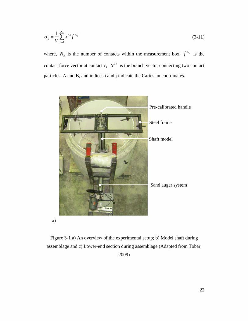
Figure 3-1 a) An overview of the experimental setup; b) Model shaft during assemblage and c) Lower-end section during assemblage (Adapted from Tobar, 2009) .................................................................................................. 22
Figure 3-2 Flowchart of DE simulation ................................................................ 24 Figure 3-3 Interaction between two DE particles ................................................. 24 Figure 3-4 The multi-layer gravitational packing procedure ................................ 27 Figure 3-5 Grain size distributions ....................................................................... 28 Figure 3-6 a) Three-dimensional direct shear sample and b) Three-dimensional
contact force network (at shear displacement of 2 m) .................................. 32 Figure 3-7 Direct shear test results ....................................................................... 33 Figure 3-8 Boundary conditions and 3D views of the model shaft ...................... 36 Figure 3-9 Initial earth pressures on the shaft ....................................................... 37 Figure 3-10 Earth pressures on the shaft at different depths (test T5) .................. 39 Figure 3-11 Earth pressures on the shaft at different depths (test T6) .................. 39 Figure 3-12 Earth pressures on the shaft at different depths (test T7) .................. 40 Figure 3-13 Earth pressures on the shaft at different depths (DEM simulation) .. 40 Figure 3-14 Normalized pressures on the shaft at the depth 0.24H ...................... 41 Figure 3-15 Normalized pressures on the shaft at the depth 0.49H ...................... 41 Figure 3-16 Normalized pressures on the shaft at the depth 0.84H ...................... 42 Figure 3-17 Comparison between modeled results and theoretical earth pressures
along the shaft. a) Shaft movement = 1 mm and b) Shaft movement = 4 mm....................................................................................................................... 45
Figure 3-18 Displacement field at shaft movement of 3 mm. .............................. 46 Figure 3-19 Contact force networks ..................................................................... 47 Figure 3-20 Stresses acting on a soil element ....................................................... 48 Figure 3-21 a) Radial stress distribution at the depth 0.49H and b) Radial stress
distribution in the cross section A-A (s = 3 mm) .......................................... 50 Figure 3-22 a) Circumferential stress distribution at the depth 0.49H and b)
Circumferential stress distribution in the cross section A-A (s = 3 mm) ..... 51 Figure 3-23 Stresses at the depth 0.49H and shaft movement 2 mm .................... 52
Figure 4-1 Flowchart of dynamic explicit FE simulation ..................................... 61 Figure 4-2 Coupling FEM and DEM using interface elements ............................ 64 Figure 4-3 Forces transmitting to FE nodes through DE particle-interface element
interaction ..................................................................................................... 64
xiii
Figure 4-4 Multi-time step algorithm ................................................................... 65 Figure 4-5 Flow chart of the coupled Finite-Discrete element method ................ 65 Figure 4-6 Geometry of the geogrid ..................................................................... 69 Figure 4-7 Initial DE specimen (partial view for illustration purpose) ................ 71 Figure 4-8 Pullout response of the geogrid ........................................................... 74 Figure 4-9 Horizontal Displacement along the geogrid ( vσ = 49 kPa) ................. 74 Figure 4-10 Geogrid deformation and displacement at ........................................ 76 Figure 4-11 Geogrid stress Sxx at Ux = 10 mm and vσ = 49 kPa ......................... 76
Figure 4-12 Average tensile force Pxx in the longitudinal members ( vσ = 49 kPa)....................................................................................................................... 77
Figure 4-13 Components of the pullout resistance ( vσ = 49 kPa) ........................ 80 Figure 4-14 Accumulated contribution of the transverse members to the total
bearing resistance at different locations along the geogrid ( vσ = 49 kPa) .... 80
Figure 4-15 Displacement field of the soil domain at Ux = 10 mm and vσ = 49 kPa....................................................................................................................... 83
Figure 4-16 Contact force networks within the soil around the geogrid .............. 84 Figure 4-17 Strain field within the soil domain at Ux = 10 mm and vσ = 49 kPa 85
Figure 4-18 Distribution of vertical and horizontal stresses in soil ( vσ = 49 kPa) 86
Figure 5-1 Plan view of the geogrid ..................................................................... 97 Figure 5-2 Initial geometry of the geogrid reinforced foundation ........................ 98 Figure 5-3 Partial view of the DE particle-geogrid interaction ............................ 99 Figure 5-4 Distributions of the contact orientation at initial condition .............. 102 Figure 5-5 Load-settlement curves of the geogrid reinforced foundation .......... 105 Figure 5-6 Geogrid vertical displacement at foundation pressure q = 125 kPa . 106 Figure 5-7 Geogrid stress Sxx at foundation pressure q = 125 kPa .................... 107 Figure 5-8 a) Vertical displacements of the geogrid (N = 1) .............................. 108 Figure 5-9 a) Maximum vertical displacements of geogrids .............................. 109 Figure 5-10 Soil displacement field of the unreinforced foundation .................. 112 Figure 5-11 Soil displacement field of the reinforced foundation (N = 1) ......... 113 Figure 5- 12 Contact force networks within the soil ........................................... 114 Figure 5-13 Vertical stress distributions beneath the strip foundation ............... 115 Figure 6-1 Initial geometry of the geogrid reinforced fill above void ................ 123 Figure 6-2 Plan view of the geogrid ................................................................... 124 Figure 6-3 Vertical displacement and tensile stress of the geogrid .................... 128 Figure 6-4 Distributions of vertical displacement and tensile stress along the
geogrid ........................................................................................................ 129
xiv
Figure 6-5 Soil displacement fields .................................................................... 130 Figure 6-6 Distributions of the contact orientation–unreinforced fill ................. 131 Figure 6-7 Distributions of the contact orientation–reinforced fill ..................... 132 Figure 6-8 Percentage porosity changes in the unreinforced and reinforced fills
.................................................................................................................... 133 Figure 6-9 Stress distributions in the unreinforced fill ....................................... 134 Figure 6-10 Stress distributions in the reinforced fill ......................................... 135
Figure A-1 Linux terminal to start YADE .......................................................... 144 Figure A-2 Controller and graphical interface .................................................... 145 Figure A-3 A cloud of spherical particles generated using makeCloud() ........... 149 Figure A-4 Snapshot of a clump and a wall ........................................................ 151 Figure A-5 Two DE particles over a FE plate. The plate is covered with triangular
interface elements to assure its interaction with DE particles .................... 154 Figure A-6 Typical simulation loop of DE simulation ....................................... 160 Figure A-7 The box and sphere described in problem 1 ..................................... 163 Figure A-8 Typical simulation loop of FE simulation ........................................ 164 Figure A-9 FE simulation of a square footing problem in YADE ...................... 167 Figure A-10 Flowchart of the coupled FE-DE framework ................................. 168 Figure A-11 Deformation of a FE plate in interaction with two DE particles using
the coupled FE-DE framework ................................................................... 171 Figure A-12 Soil sample in problem 4 before and after compression ................ 175 Figure A-13 DE used in the three-dimensional direct shear test and b) Three-
dimensional contact force network ............................................................. 179 Figure A-14 a) Initial geometry of the geogrid reinforced foundation b) Partial
view of the DE particle-geogrid interaction ............................................... 184 Figure A-15 Initial DE specimen for the geogrid pulout test (partial view for
illustration purpose) .................................................................................... 188 Figure A-16 Initial sample geometry for problem 8 ........................................... 192 Figure A-17 Displacement field in the soil domain (problem 6) ........................ 195 Figure A-18 Distributions of contact orientation (problem 6) ............................ 196 Figure A-19 Vertical stress distribution (problem 6) .......................................... 199 Figure A-20 Tensile stress of a geogrid during pullout test (problem 7) ............ 200 Figure A-21 Deformation of the buried pipe and the FE soil domain (problem 8)
.................................................................................................................... 200 Figure A-22 Strain field in the soil domain (problem 7) .................................... 201
xv

LIST OF TABLES
Table 3-1 Soil properties used in the experimental study ..................................... 19 Table 3-2 Particles' properties for DE simulations ............................................... 31 Table 4-1 Input parameters for the simulation ...................................................... 68 Table 5-1 Input parameters for the simulation ...................................................... 96 Table 6-1 Input parameters for the simulation .................................................... 122
xvi

LIST OF SYMBOLS
Roman Symbols
a Radius of the model shaft
B Width of the strip foundation
c Damping coefficient for the mass proportional damping
Cu Soil coefficient of uniformity
Cc Soil coefficient of curvature
D Model shaft diameter
d0 Distance between two particle centers
D5 Particle diameter corresponding to 5 % passing
D50 Particle diameter corresponding to 50 % passing
Dr Relative density
E Particle material modulus
Fbt Bearing resistance of geogrid transverse members jcf , Contact force vector at contact point c
contactF
Total contact force
Ff Geogrid frictional resistance
NF
Normal force of a contact
Fp Total geogrid pullout resistance
TF
Tangential force of a contact
h Depth of a earth pressure measurement point
H Height of a soil domain
i, j Cartesian coordinates
K Sum of normal stiffnesses of all particles interacting with a wall
K Stiffness matrix
xvii
iK Per-particle stiffness of contacts in which particle i participates
Ko Lateral earth pressure coefficient at-rest
KN Normal stiffness at a contact
Kr Rolling stiffness of an interaction
KT Tangential stiffness at a contact ( )Ank Normal stiffness of particle A
( )Bnk Normal stiffness of particle B
M Mass matrix
im Mass of particle i
rM
Resistant moment
N Coordination number, number of geogrid layers
Nc Number of contacts within a measurement box
ni Unit branch vector component in the i direction
iN Shape functions
Np Number of particles
p Active earth pressure acting on a vertical shaft
P External force vector
P0 Initial earth pressure acting on a vertical shaft
Pxx Average tensile force
q Foundation pressure
rA, rB Radii of particles A and B
s Shaft radius reduction
Sxx Stress in the x-direction within the geogrid
Ux Geogrid frontal displacement
V Volume of a measurement rectangular box
x Displacement vector
icx , Branch vector connecting two contact particles
xviii

( )ix Coordinate of node i of a quadrilateral
)(Ox Temporary center node
Greek Symbols
α The angle that the failure surface makes with the horizontal
rβ Rolling resistance coefficient
γ Soil unit weight
TδΔ
Incremental tangential displacement
Tδ F
Incremental tangential force
Δ Contact penetration depth
crt∆ Critical time-step
FEt∆ Time-step in the finite element domain
DEt∆ Time-step in the discrete element domain
NΔ
Normal penetration between two particles
rη A dimensionless coefficient
λ Earth pressure coefficient on the radial plane
mλ Maximum eigenvalue
rθ
Rolling angular vector
ν Poisson's ratio
σ , vσ Current normal stress acting on a wall
ijσ Average stresses within a box
0σ Desired normal stress acting on a wall
xix
θσ Circumferential stress in soil
rσ Radial stress in soil
zσ Vertical stress in soil
microϕ Microscopic friction angle
φ Internal friction angle (deg)
ijΦ Fabric tensor
xx
CHAPTER 1
Introduction
1.1. Introduction
The interaction between soil and geotechnical structures has been attracting
enormous research attention in the last few decades. Beside experimental studies,
numerical methods have proven to be efficient in modeling the soil-structure
interaction at the macroscopic scale level. The finite element method (FEM) has
been widely used to model soil-structure interaction in many geotechnical
engineering problems including tunneling process (Mroueh and Shahrour, 2002),
deep excavation (Zdravkovic et al., 2005) and pile foundation (Karthigeyan et al.,
2007). However, it is challenging for standard finite element methods to properly
model the soil-structure interaction at the particle scale level. For geotechnical
engineering problems that involve particle movement such as void erosion around
tunnel lining (Meguid and Dang, 2009), earth pressure on cylindrical shaft (Tobar
and Meguid, 2011) and geogrid reinforcement (Michalowski, 2004), the soil-
structure interaction nature may not be properly captured using FEM.
The discrete element method (DEM) has proven to be promising for modeling
geotechnical engineering problems which involve granular material and large
deformation (Herten and Pulsfort, 1999; Cui and O'Sullivan, 2006; Guerrero et
al., 2006). Although DEM is considered efficient in modeling soil particles, it is
challenging to properly model the behavior of structural elements using discrete
particles due to the continuum behavior of the structure. The coupling of the finite
and discrete element methods, which takes advantages of the two methods, is a
promising approach for modeling soil-structure interaction.
1
1.2. Research Motivation
Although the coupling of FEM and DEM was initially used by researchers to
solve dynamic impact problems (Han et al., 2002; Xiao and Belytschko, 2004;
Dhia and Rateau, 2005; Bhuvaraghan et al., 2010), little work has been done to
develop a coupling approach in geotechnical engineering. A two-dimensional
coupled FE-DE framework was proposed by Onate and Rojek (2004) to solve
dynamic geotechnical engineering problems. Fakhimi (2009) proposed a
combined method to simulate triaxial tests by using finite elements to model the
membrane and discrete elements to model the soil sample. The simulation
required a very fine FE mesh with a large number of elements to maintain
numerical stability. Coupled FE-DE simulations reported by Villard et al. (2009),
Elmekati and Shamy (2010) and Dang and Meguid (2013) were not validated with
experimental data.
Thus, the goal of the thesis is to develop a coupled FE-DE framework suitable for
soil-structure interaction analysis validated using experimental data. This involves
developing a new DEM packing method, simulating DE problems, and
conducting soil-structure interaction analysis using the developed FE-DE
framework.
1.3. Objective and Scope
The research presented in this thesis has two major objectives. The first objective
is to validate the use of the discrete element method in investigating geotechnical
engineering problems involving large deformation. This objective is achieved by
addressing the following:
1) Develop a gravitational packing method to simulate the soil deposition.
2) Investigate the earth pressure distribution on cylindrical shaft in soft
ground using the discrete element method. The numerical simulation is
validated by comparing the numerical results with experimental data.
2
The second objective is to develop a coupled Finite-Discrete element framework
and use the framework to investigate geotechnical engineering problems
involving soil-structure interaction and granular material. This is achieved by
addressing the following:
3) Develop a coupled Finite-Discrete element framework and implement the
developed framework into an open source code.
4) Analyze pullout test of biaxial geogrid embedded in granular material.
5) Analyze strip footing over geogrid-reinforced sand.
6) Analyze geogrid-reinforced fill over strong formation containing void.
1.4. Contributions of authors
Papers J1, J2, J3, C1, C2, C3, C4 and C5 listed in the publication list are included
in the thesis. All papers are the candidate’s original work.
The coupled Finite-Discrete element framework developed in the thesis is a
continuation of the original work of Dang and Meguid (2010, 2013). Dang
developed the initial framework and used it to simulate a tunnelling process. The
author has moved the original finite element engines into a new version of the
open source discrete element code YADE. Original C++ codes were modified by
the author in order to make them compatible with the new version of YADE.
Bugs detected from the original framework have been fixed. New C++ engines
for discrete and finite element as well as coupled Finite-Discrete element analyses
used in the thesis are written by the author. The author has wrapped all developed
C++ engines in Python, a scripting language in YADE. This assures rapid and
flexible simulation process. A manual for the developed coupled Finite-Discrete
element framework written by the author is presented in the appendix of the
thesis.
All the formulation, program coding, and the preparation of the manuscripts were
completed by the candidate, under the supervision of Prof. Mohamed Meguid and
Prof. Luc Chouinard, his thesis supervisors.
3
1.5. Thesis Organization
This thesis consists of seven chapters. The chapters essentially reflect the order in
which the research was carried out. Chapter 2 presents recent developments in
modeling soil-structure interaction problems involving granular material and large
deformation. Chapters 3 and 4 are modified versions of journal papers J1 and J2
while chapter 5 and 6 are parts of journal paper J3 in the publication list.
Chapter 3 illustrates the advantages of the discrete element method in modeling
geotechnical engineering problems involving granular material and large
deformation. In this chapter, numerical studies that have been conducted to
investigate the earth pressure distribution on cylindrical shaft in soft ground are
presented. Previous experimental work conducted by the research group is
summarized first. The experiment consists of a mechanically adjustable lining
installed in granular material under axisymmetric condition. The shaft radius is
gradually reduced and the earth pressure acting on the shaft is measured for
different induced wall movements. A discrete element analysis is then performed
to simulate the experiment using a new gravitational packing. Input parameters
for the simulation are determined using experimental results of direct shear tests.
The microscopic behavior of the soil domain is obtained from the discrete element
simulation. The chapter is a modified version of paper J1 in the publication list.
Chapter 4 presents the coupled Finite-Discrete element framework developed to
simulate soil-structure interaction. Force transmission between the finite and
discrete element domains is assured using interface elements. Explicit time
integration is used in both the finite and discrete element calculations. Different
damping schemes are applied to each domain to relax the system. A multiple-
time-step scheme is applied to optimize the computational cost. The developed
coupled Finite-Discrete element framework is used to investigate a pullout test of
a biaxial geogrid embedded in granular material. The geogrid is modeled using
finite elements while the soil is modeled using discrete elements. The results of
the analysis are compared with experimental data. The displacements and stresses
4
developing in the geogrid as well as the micro-mechanical behavior of the soil
domain are investigated. The proposed coupled Finite-Discrete element method
has proven its efficiency in modeling pullout test in three-dimensional space and
capturing the response of both the geogrid and the surrounding material. The
chapter presents the work carried out in paper J2 in the publication list.
Chapter 5 investigates the behavior of a strip foundation over geogrid reinforced
sand using the developed coupled Finite-Discrete element framework. The
numerical simulation is validated by comparing the numerical results with the
experimental data and the soil-geogrid interlocking effect is demonstrated. The
deformation and stress distribution within the geogrid as well as the behavior of
the soil domain relative to soil displacements, contact orientations, contact forces
are also analyzed. The proposed coupled Finite-Discrete element method has
demonstrated its efficiency in investigating the three-dimensional soil-geogrid
interaction at the microscopic scale. The chapter is part of paper J3 in the
publication list.
Chapter 6 presents a numerical simulation of geogrid-reinforced fill over strong
formation containing void using the proposed coupled Finite-Discrete element
framework. The backfill soil is modeled using discrete elements while the geogrid
is modeled using finite elements. The use of geogrid to reinforce a fill over a void
is proven to be effective in preventing soil from moving toward the void. The
developed coupled Finite-Discrete element framework efficiently captures the
deformations and stresses of the geogrid as well as the soil displacements, contact
orientations, stresses and porosity changes. The chapter is part of paper J3 in the
publication list.
Conclusions drawn from this research and recommendations for future research
are outlined in chapter 7.
5
CHAPTER 2
Literature Review
Literature related to the modeling of soil-structure interaction in geotechnical
engineering as well as the available techniques to couple the finite and discrete
element methods are summarized below.
2.1. Soil-Structure Interaction Modeling using the Finite Element Method
The finite element method has been widely used to model soil-structure
interaction in many geotechnical engineering problems such as tunneling, deep
excavation and pile foundation. Modeling the tunneling process using FEM has
been performed by researchers including Mroueh and Shahrour (2002), Galli et al.
(2004), Kasper and Meschke (2004), Meguid and Rowe (2006) and Yoo (2013).
Soil-wall interaction during excavation process has been studied by Faheem et al.
(2004), Zdravkovic et al. (2005) and Finno et al. (2007). Similarily, FEM has
been used to model soil-pile interaction (Pan et al., 2002; Khodair et al., 2005;
Maheshwari et al., 2005; Karthigeyan et al., 2007). Soil-structure interaction is
often assured using interface elements (Bfer, 1985; Van Langen and Vermeer,
1991; Karabatakis and Hatzigogos, 2002). In the above studiess, the soil-structure
interactions using interface elements were often considered at the macroscopic
scale.
In geotechnical engineering problems such as those involving erosion voids next
to tunnel lining (Zienkiewicz and Huang, 1990; Meguid and Dang, 2009), earth
pressure on cylindrical shaft (Berezantzev, 1958; Tobar and Meguid, 2011) and
geogrid reinforced soil (Agaiby et al., 1995; Palmeira, 2004; Michalowski, 2004),
it is necessary to model the soil-structure interaction at the particle scale level to
properly capture the soil particle-structure interaction. Voids due to erosion
around tunnel linings often have irregular shapes and sizes and it is challenging to
6
model the void development using FEM especially when the void size increases
(Meguid and Dang, 2009). The active earth pressure on a cylindrical shaft is
generally reached with sufficient shaft wall movement. For the case of a shaft
surrounded by granular soil, the required shaft movement to reach the full active
condition was found to range from 2.5% to 4% of the shaft radius (Tran et al.,
2012). The problem involves granular material and large deformation which
makes it challenging to properly capture the earth pressure acting on the shaft
wall using traditional FEM. In reinforced soil problems such as geogrid pullout
test (Palmeira, 2004), geogrid reinforced foundation (Michalowski, 2004) and
geogrid reinforced fill over void (Agaiby et al., 1995), soil-geogrid interlocking
effect is considered an important feature. However, it is challenging to model the
interlocking effect using FEM due to its particle based interaction. Moreover, the
geogrid geometry is often simplified either as a truss structure (in 2D analysis) or
a continuous sheet (in 3D analysis) which ignores the interlocking effect.
Although the above soil-structure interaction problems may be modeled using an
adaptive remeshing approach (Zienkiewicz and Huang, 1990; Zienkiewicz et al.,
1995) or a multiscale approach (Hughes, 1995; Garikipati and Hughes, 1998),
numerical simulations involving large soil deformation and unpredictable
discontinuities using these approaches did not receive much research attention in
the literature.
2.2. Granular Modeling using the Discrete Element Method
The discrete element method has proven to be a promising approach to capture
the response of granular material experiencing large deformation. The method
was first proposed by Cundall and Strack (1979) and has been widely used to
analyze geotechnical problems. In this method, a soil domain is modeled using a
set of discrete particles interacting at their contact points. Particles can have
different shapes such as discs, spheres, ellipsoids and clumps. The real grain size
distribution can be modeled using particles with variable sizes. The interaction
between particles is regarded as a dynamic process that reaches static equilibrium
7
when the internal and external forces are balanced. The dynamic behavior is
represented by a time-step algorithm using an explicit time-difference scheme.
Newton's and Euler's equations are used to determine particle displacement and
rotation.
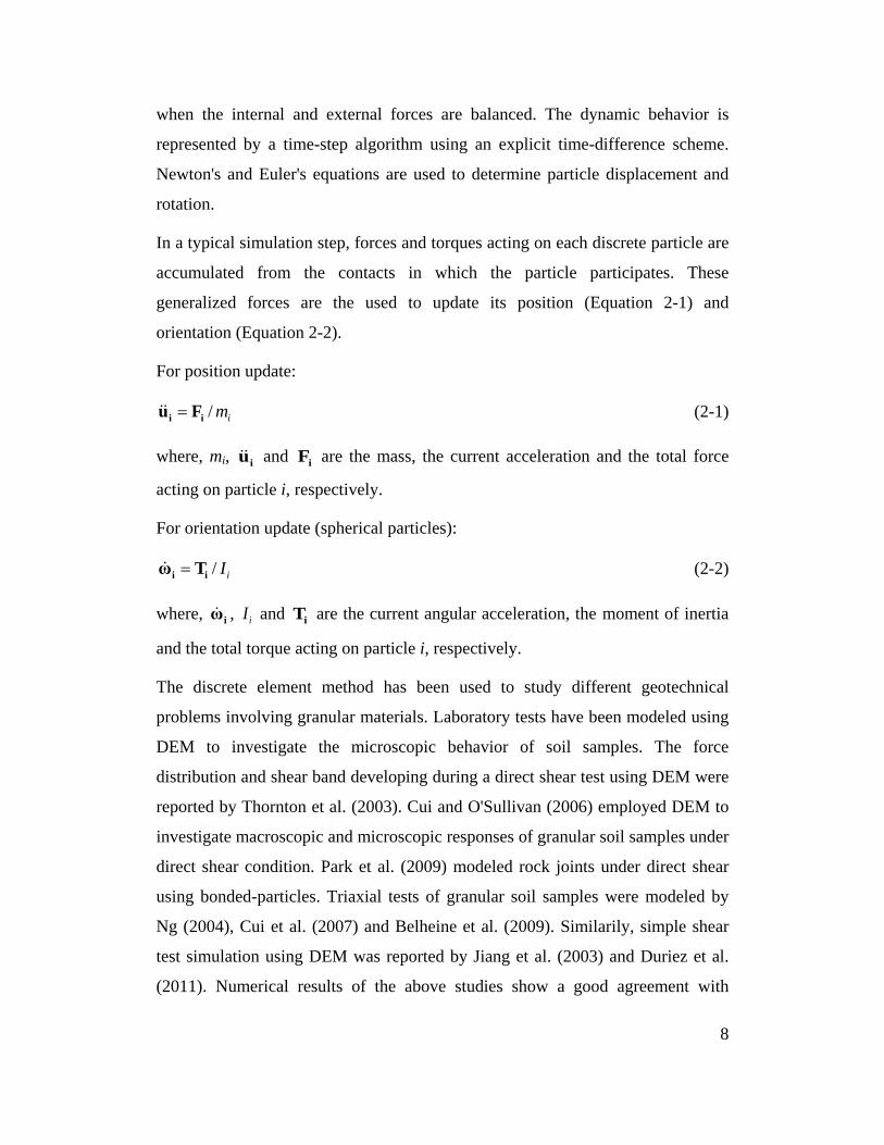
In a typical simulation step, forces and torques acting on each discrete particle are
accumulated from the contacts in which the particle participates. These
generalized forces are the used to update its position (Equation 2-1) and
orientation (Equation 2-2).
For position update:
im/ii Fu = (2-1)
where, mi, iu and iF are the mass, the current acceleration and the total force
acting on particle i, respectively.
For orientation update (spherical particles):
iI/ii Tω = (2-2)
where, iω , iI and iT are the current angular acceleration, the moment of inertia
and the total torque acting on particle i, respectively.
The discrete element method has been used to study different geotechnical
problems involving granular materials. Laboratory tests have been modeled using
DEM to investigate the microscopic behavior of soil samples. The force
distribution and shear band developing during a direct shear test using DEM were
reported by Thornton et al. (2003). Cui and O'Sullivan (2006) employed DEM to
investigate macroscopic and microscopic responses of granular soil samples under
direct shear condition. Park et al. (2009) modeled rock joints under direct shear
using bonded-particles. Triaxial tests of granular soil samples were modeled by
Ng (2004), Cui et al. (2007) and Belheine et al. (2009). Similarily, simple shear
test simulation using DEM was reported by Jiang et al. (2003) and Duriez et al.
(2011). Numerical results of the above studies show a good agreement with
8
experimental data which demonstrates the efficiency of DEM in simulating
laboratory tests.
Large scale geotechnical problems have been also modeled using DEM. Lobo-
Guerrero et al. (2006) investigated the behavior of railtrack ballast degradation
during cyclic loading. The particle breakage process was visualized and the effect
of crushing on the behavior of track ballast material was investigated. Bearing
capacity of driven piles in crushable granular materials was studied by Lobo-
Guerrero and Vallejo (2005) using breakable DE particles. Deluzarche and
Cambou (2006) employed the same approach to study rockfill dam behavior.
Those simulations were capable of simulating particle breakage process which is
difficult to observe using experimental tests.
Earth pressure acting on vertical shafts was studied by Herten and Pulsfort (1999).
Spherical particles were used to model the soil domain. The circular shaft was
assumed to behave as segments made from small flat walls. The shaft wall was
gradually moved inward and lateral pressures acting on the shaft wall were
recorded. Results of the numerical simulation were then compared with
experimental data.
A simplified DEM model was developed by Maynar et al. (2005) to study the
underground tunneling process. Input parameters for the numerical simulation
were determined using triaxial test calibration. The excavation process was
modeled and the tunnel face stability was analyzed. The thrust and torque
evolution with respect to the movement of earth pressure balance machine were
investigated.
Gabrieli et al. (2009) studied the behaviour of a shallow foundation on a model
slope. A particle upscale approach was proposed to reduce the number of DE
particles required for the simulation. Displacement fields and contact force
networks of the model were obtained at the microscopic level.
Jenck et al. (2009) employed DEM to model granular fill supported by piles. A
simplified two-dimensional DE model was developed to investigate soil
9
improvement using vertical rigid piles. Macro scale responses of the platform
over piles such as soil arching, loads transfer to the piles and platform settlement
were analyzed. The DE simulation was compared with experimental data.
Parametric studies were performed to investigate the influence of microscopic
parameters on the macroscopic response of the model.
It can be seen that although DE simulations have been reported in the literature,
the number of DE validations is still limited and needs to be expanded. Moreover,
the studied DE models were often simplified in 2D space (Lobo-Guerrero and
Vallejo, 2005; Deluzarche and Cambou, 2006; Lobo-Guerrero et al., 2006; Jenck
et al., 2009) which limits the capability of DEM to capture the 3D soil behavior at
the microscopic level.
The modeling of soil-structure interaction using DEM has been reported by
Villard and Chareyre (2004), McDowell et al. (2006), Han et al. (2011) and Chen
et al. (2012). Villard and Chareyre (2004) used two-dimensional DEM to model
the failure of geosynthetic sheets anchored in trenches. The geosynthetic sheets
were modeled using "dynamic spar elements" while backfill soil was modeled
using disk elements. Contact laws between dynamic spar elements and disks were
introduced to assure their interaction. Pullout strengths of different anchorage
shapes as well as deformation and failure mechanism of the system were
investigated.
McDowell et al. (2006) and Chen et al. (2012) used DEM to model both the
geogrid and the backfill soil. The geogrid was modeled using a set of spherical
particles bonded together to form the geogrid shape. The interaction between the
geogrid and the surrounding soil was obtained through the contact between
discrete particles. The geogrid was then pulled out to investigate the peak
mobilised resistance and associated displacement (McDowell et al., 2006). In
Chen et al. (2012), the behavior of the geogrid-reinforced ballast under cyclic
loading was investigated and the effectiveness of the geogrid reinforcement was
examined.
10
Han et al. (2011) used DEM to model geogrid-reinforced embankment over piles.
The 2D embankment was modeled using disk elements and the 2D geogrid was
modeled using bonded particles. The changes of stresses, porosities and
displacements within the embankment fill as well as the behavior of the geogrid
were investigated.
In the above soil-structure interaction simulations, the structural elements were
modeled using dynamic spar elements or bonded particles which do not represent
the continuous nature of the structure. Moreover, due to the inflexibility of the
bonded particles and dynamic spar elements, the real deformation as well as
strains and stresses within the structure may not be accurately captured.
2.3. Coupling the Finite and Discrete Element Methods
To take advantage of both FEM and DEM, the coupling of the two numerical
methods has been proposed. In this approach, the analyzed problem is divided
into FE and DE domains. Several algorithms have been developed to assure the
load transfer from the FE domain to DE domain and vice versa.
A procedure for combining finite and discrete elements to simulate the shot
peening process was proposed by Han et al. (2002). Spherical shot was modeled
using rigid discrete elements while the target material was modeled using
deformable finite elements. The developed algorithm could capture the dynamic
nature of the shot peening. However, the element size in the impact area should be
no larger than d/10 where d is the diameter of the shot. This requires a large
number of finite elements which results in high computational cost. A simulation
of the shot peening process using a combined finite-discrete element approach
was also reported by Bhuvaraghan et al. (2010).
An algorithm for coupling the finite and discrete element methods was reported
by Fakhimi (2009). The algorithm was capable of modeling deformable
membrane in a laboratory triaxial test. The membrane was modeled using FE
while the soil was modeled using DE. The membrane-soil interaction was based
11
on the contact between DE and external face of the FE membrane. Both FE and
DE computations were integrated explicitly using a central difference scheme.
Xiao and Belytschko (2004) proposed a bridging domain method for coupling
continuum models with molecular models. In this approach, the continuum and
molecular domains were overlapped in a bridging sub-domain. Using the
linearization of Halmitonian dynamics for both molecular and continuum models,
this multi-scale method can avoid spurious wave reflections at the
molecular/continuum interface. A multiple-time-step algorithm was also proposed
within this framework. Similar techniques to combine the finite and discrete
element domains were reported by Dhia (1998) and Dhia and Rateau (2005).
Although the above coupling approaches have shown their efficiency in analyzing
certain engineering problems, their applications in geotechnical engineering are
still very limited. Villard et al. (2009) proposed a coupled FE-DE approach to
model earth structures reinforced by geosynthetic. Interface elements were
proposed to assure the interaction between the FE and DE domains. The
framework was used to model the interaction between a geosynthetic sheet and
surrounding soil. The geosynthetic sheet was modeled using FE while the soil was
modeled using DE. Elmekati and Shamy (2010) used a similar approach to model
a rigid pile in contact with granular soil. The near-field zone surrounding the pile
was modeled using DE whereas FE was used to model far-field zones. The
interaction between the FE and DE domains was assured using a wall set of
polygons having the same geometry of finite element surfaces at the interface.
Dang and Meguid (2013) proposed a coupled FE-DE approach to model soil-
structure interaction problems involving large deformation. The domain involving
the large deformation was modeled using DE while FE was used to model the rest
of the domain. Interface elements at the boundary of the two domains were
introduced to transmit interacting forces between the DE and FE domains.
Explicit time integration with different damping schemes were applied to each
domain in order to relax the system and to reach the convergence condition. Since
12
a relatively coarse FE mesh is required, the algorithm reduces the computational
time. The framework was then used to simulate a soft ground tunneling problem
involving soil loss near an existing lining.
2.4. Conclusion for the Literature Review
Based on the previous literature review and in addition to the review presented in
the coming chapters, it can be seen that little work has been done to date to
validate discrete element simulations of problems particularly those involving
granular material and large deformation. Although the coupled finite-discrete
element approach has been used in geotechnical engineering to model certain soil-
structure interaction problems, the available validation of the coupling approach is
still very limited. Therefore, there is a need to model and validate complicated
soil-structure interaction problems such as those of three-dimensional soil-geogrid
interaction. It is also necessary to develop an efficient coupled finite-discrete
element framework that reduces computational cost and modeling effort. Such
development will be presented in this thesis along with experiments and
numerical simulations of geotechnical engineering problems.
13
CHAPTER 3
Discrete Element Simulation and Experimental Study of the Earth Pressure Distribution on Cylindrical Shafts *
Abstract
Experimental and numerical studies have been conducted to investigate the earth
pressure distribution on cylindrical shafts in soft ground. A small scale laboratory
setup that involves a mechanically adjustable lining diameter installed in granular
material under axisymmetric condition is first described. The earth pressure acting
on the shaft and the surface displacements are measured for different induced wall
movements. A numerical modeling is then performed using the discrete element
method to allow for the simulation of the large soil displacement and particle
rearrangement near the wall. The experimental and numerical results are
summarized and compared against previously published theoretical solutions.
Conclusions regarding the soil failure and the pressure distributions in both the
radial and circumferential directions are presented.
Keywords: discrete element method, cylindrical shaft, earth pressure, retaining
structures.
* A version of this chapter has been published in International Journal of
Geomechanics ASCE, 2012 (in press).
14
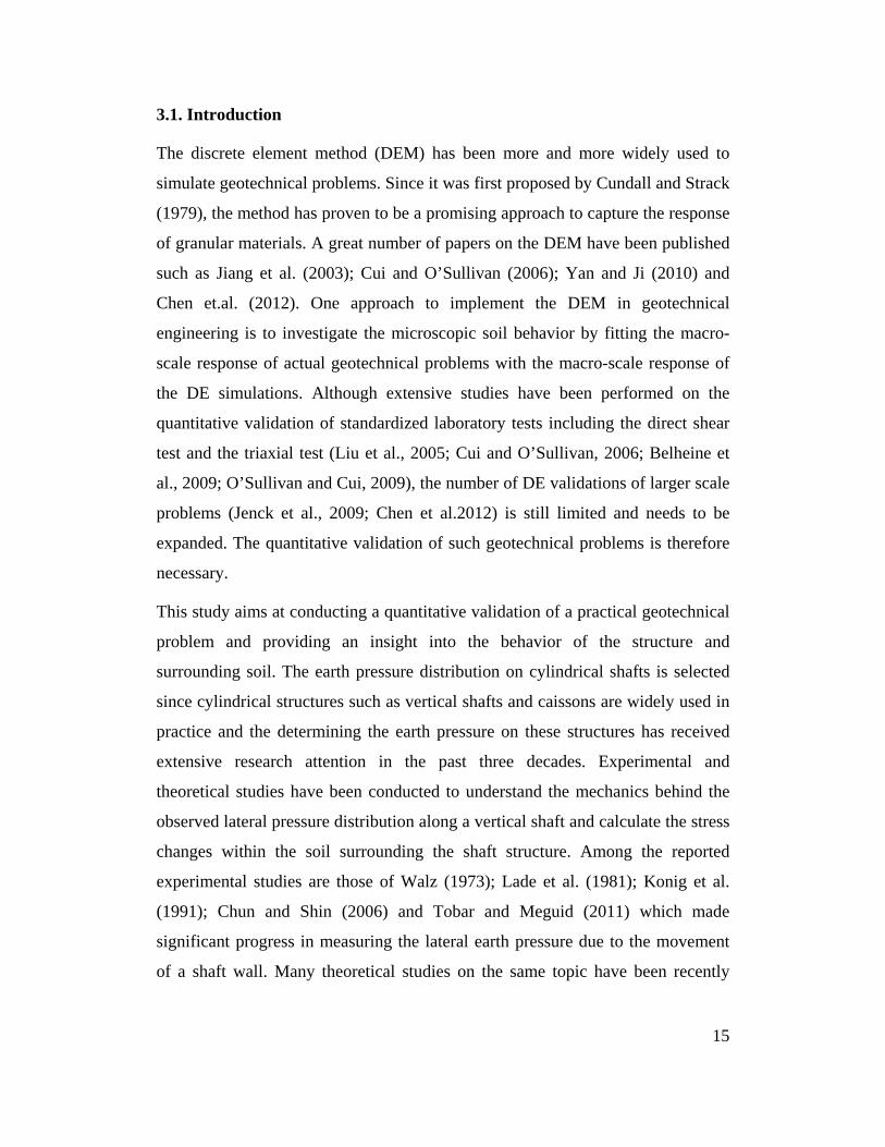
3.1. Introduction
The discrete element method (DEM) has been more and more widely used to
simulate geotechnical problems. Since it was first proposed by Cundall and Strack
(1979), the method has proven to be a promising approach to capture the response
of granular materials. A great number of papers on the DEM have been published
such as Jiang et al. (2003); Cui and O’Sullivan (2006); Yan and Ji (2010) and
Chen et.al. (2012). One approach to implement the DEM in geotechnical
engineering is to investigate the microscopic soil behavior by fitting the macro-
scale response of actual geotechnical problems with the macro-scale response of
the DE simulations. Although extensive studies have been performed on the
quantitative validation of standardized laboratory tests including the direct shear
test and the triaxial test (Liu et al., 2005; Cui and O’Sullivan, 2006; Belheine et
al., 2009; O’Sullivan and Cui, 2009), the number of DE validations of larger scale
problems (Jenck et al., 2009; Chen et al.2012) is still limited and needs to be
expanded. The quantitative validation of such geotechnical problems is therefore
necessary.
This study aims at conducting a quantitative validation of a practical geotechnical
problem and providing an insight into the behavior of the structure and
surrounding soil. The earth pressure distribution on cylindrical shafts is selected
since cylindrical structures such as vertical shafts and caissons are widely used in
practice and the determining the earth pressure on these structures has received
extensive research attention in the past three decades. Experimental and
theoretical studies have been conducted to understand the mechanics behind the
observed lateral pressure distribution along a vertical shaft and calculate the stress
changes within the soil surrounding the shaft structure. Among the reported
experimental studies are those of Walz (1973); Lade et al. (1981); Konig et al.
(1991); Chun and Shin (2006) and Tobar and Meguid (2011) which made
significant progress in measuring the lateral earth pressure due to the movement
of a shaft wall. Many theoretical studies on the same topic have been recently
15
reported such as Cheng and Hu (2005); Cheng et al. (2007); Salgado and Prezzi
(2007); Andresen et al. (2011) and Osman and Randolph (2012).
An attempt has been made by Herten and Pulsfort (1999) to apply the DEM to
simulate a laboratory size shaft construction. Although the study provided useful
results, the circular shaft was assumed to behave as a small flat wall which has
lead to an inadequate simulation of the arching effect and the stress distribution
around the shaft. Furthermore, a quite small segment of the shaft geometry was
modeled resulting in the presence of rigid boundaries close to the investigated
area. Therefore, there is a need for an improved DE simulation of the problem
considering the problem geometry as well as realistic soil properties.
In this paper, an experimental study of a model shaft installed in granular material
is first presented. The recorded lateral earth pressures acting on the shaft with
different wall movements is measured. A DE model that has been developed to
simulate the shaft model is then introduced. A suitable packing method to
generate the soil domain is proposed and a calibration test is conducted to
determine the input parameters needed for the simulation. The results of the
experimental and numerical studies are then analyzed and conclusions are made
regarding the distribution of the radial and circumferential stresses around the
shaft as well as the extent of soil shear failure.
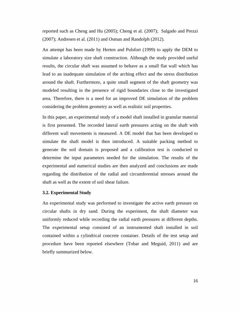
3.2. Experimental Study
An experimental study was performed to investigate the active earth pressure on
circular shafts in dry sand. During the experiment, the shaft diameter was
uniformly reduced while recording the radial earth pressures at different depths.
The experimental setup consisted of an instrumented shaft installed in soil
contained within a cylindrical concrete container. Details of the test setup and
procedure have been reported elsewhere (Tobar and Meguid, 2011) and are
briefly summarized below.
16
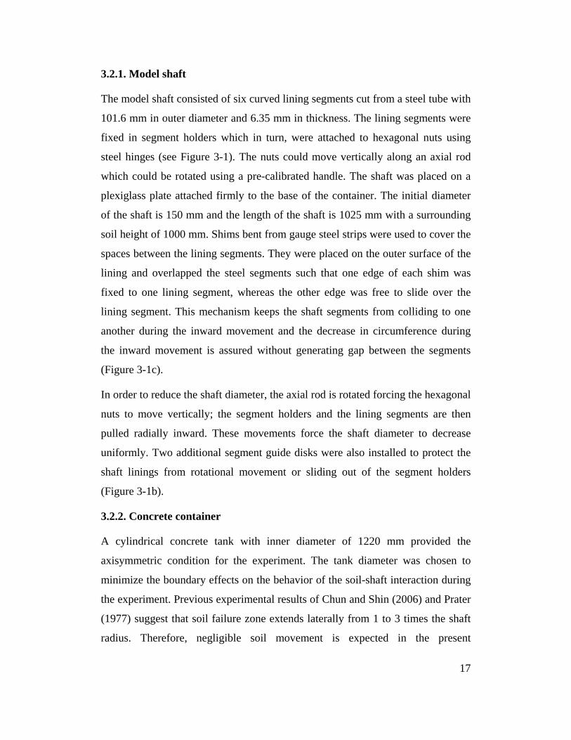
3.2.1. Model shaft
The model shaft consisted of six curved lining segments cut from a steel tube with
101.6 mm in outer diameter and 6.35 mm in thickness. The lining segments were
fixed in segment holders which in turn, were attached to hexagonal nuts using
steel hinges (see Figure 3-1). The nuts could move vertically along an axial rod
which could be rotated using a pre-calibrated handle. The shaft was placed on a
plexiglass plate attached firmly to the base of the container. The initial diameter
of the shaft is 150 mm and the length of the shaft is 1025 mm with a surrounding
soil height of 1000 mm. Shims bent from gauge steel strips were used to cover the
spaces between the lining segments. They were placed on the outer surface of the
lining and overlapped the steel segments such that one edge of each shim was
fixed to one lining segment, whereas the other edge was free to slide over the
lining segment. This mechanism keeps the shaft segments from colliding to one
another during the inward movement and the decrease in circumference during
the inward movement is assured without generating gap between the segments
(Figure 3-1c).
In order to reduce the shaft diameter, the axial rod is rotated forcing the hexagonal
nuts to move vertically; the segment holders and the lining segments are then
pulled radially inward. These movements force the shaft diameter to decrease
uniformly. Two additional segment guide disks were also installed to protect the
shaft linings from rotational movement or sliding out of the segment holders
(Figure 3-1b).
3.2.2. Concrete container
A cylindrical concrete tank with inner diameter of 1220 mm provided the
axisymmetric condition for the experiment. The tank diameter was chosen to
minimize the boundary effects on the behavior of the soil-shaft interaction during
the experiment. Previous experimental results of Chun and Shin (2006) and Prater
(1977) suggest that soil failure zone extends laterally from 1 to 3 times the shaft
radius. Therefore, negligible soil movement is expected in the present
17
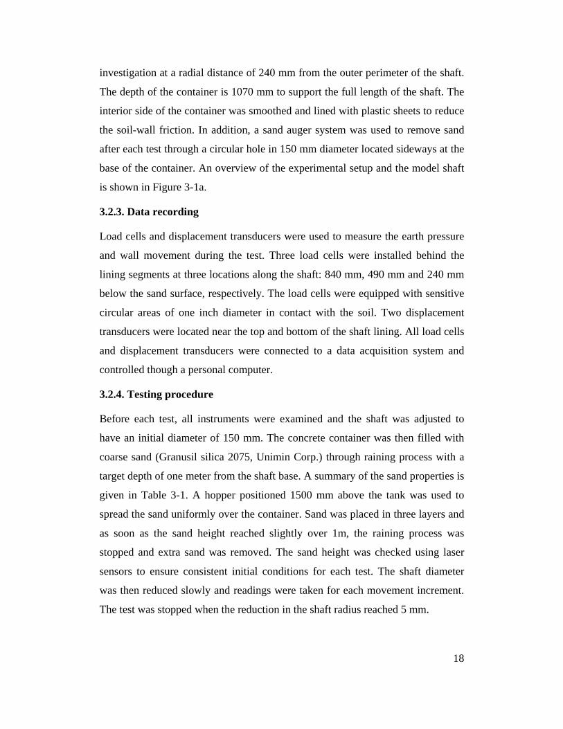
investigation at a radial distance of 240 mm from the outer perimeter of the shaft.
The depth of the container is 1070 mm to support the full length of the shaft. The
interior side of the container was smoothed and lined with plastic sheets to reduce
the soil-wall friction. In addition, a sand auger system was used to remove sand
after each test through a circular hole in 150 mm diameter located sideways at the
base of the container. An overview of the experimental setup and the model shaft
is shown in Figure 3-1a.
3.2.3. Data recording
Load cells and displacement transducers were used to measure the earth pressure
and wall movement during the test. Three load cells were installed behind the
lining segments at three locations along the shaft: 840 mm, 490 mm and 240 mm
below the sand surface, respectively. The load cells were equipped with sensitive
circular areas of one inch diameter in contact with the soil. Two displacement
transducers were located near the top and bottom of the shaft lining. All load cells
and displacement transducers were connected to a data acquisition system and
controlled though a personal computer.
3.2.4. Testing procedure
Before each test, all instruments were examined and the shaft was adjusted to
have an initial diameter of 150 mm. The concrete container was then filled with
coarse sand (Granusil silica 2075, Unimin Corp.) through raining process with a
target depth of one meter from the shaft base. A summary of the sand properties is
given in Table 3-1. A hopper positioned 1500 mm above the tank was used to
spread the sand uniformly over the container. Sand was placed in three layers and
as soon as the sand height reached slightly over 1m, the raining process was
stopped and extra sand was removed. The sand height was checked using laser
sensors to ensure consistent initial conditions for each test. The shaft diameter
was then reduced slowly and readings were taken for each movement increment.
The test was stopped when the reduction in the shaft radius reached 5 mm.
18
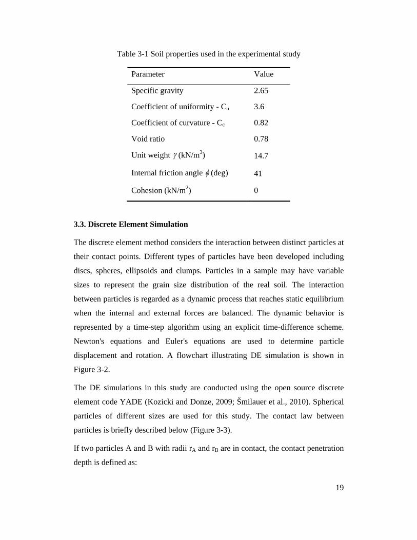
Table 3-1 Soil properties used in the experimental study
Parameter Value
Specific gravity 2.65
Coefficient of uniformity - Cu 3.6
Coefficient of curvature - Cc 0.82
Void ratio 0.78
Unit weight γ (kN/m3) 14.7
Internal friction angle φ (deg) 41
Cohesion (kN/m2) 0
3.3. Discrete Element Simulation
The discrete element method considers the interaction between distinct particles at
their contact points. Different types of particles have been developed including
discs, spheres, ellipsoids and clumps. Particles in a sample may have variable
sizes to represent the grain size distribution of the real soil. The interaction
between particles is regarded as a dynamic process that reaches static equilibrium
when the internal and external forces are balanced. The dynamic behavior is
represented by a time-step algorithm using an explicit time-difference scheme.
Newton's equations and Euler's equations are used to determine particle
displacement and rotation. A flowchart illustrating DE simulation is shown in
Figure 3-2.
The DE simulations in this study are conducted using the open source discrete
element code YADE (Kozicki and Donze, 2009; Šmilauer et al., 2010). Spherical
particles of different sizes are used for this study. The contact law between
particles is briefly described below (Figure 3-3).
If two particles A and B with radii rA and rB are in contact, the contact penetration
depth is defined as:
19
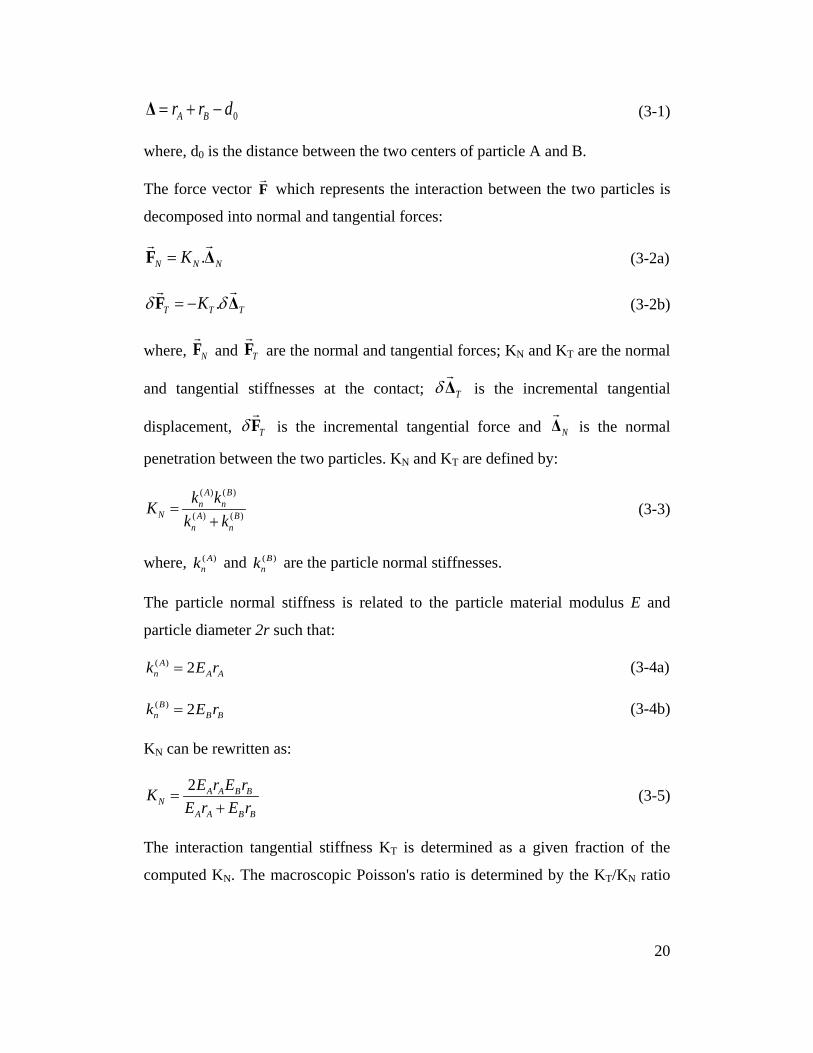
0A Br r d= + −Δ (3-1)
where, d0 is the distance between the two centers of particle A and B.
The force vector F
which represents the interaction between the two particles is
decomposed into normal and tangential forces:
.N N NK=F Δ
(3-2a)
.T T TKδ δ= −F Δ
(3-2b)
where, NF
and TF
are the normal and tangential forces; KN and KT are the normal
and tangential stiffnesses at the contact; TδΔ
is the incremental tangential
displacement, Tδ F
is the incremental tangential force and NΔ
is the normal
penetration between the two particles. KN and KT are defined by:
( ) ( )
( ) ( )
A Bn n
N A Bn n
k kKk k
=+
(3-3)
where, ( )Ank and ( )B
nk are the particle normal stiffnesses.
The particle normal stiffness is related to the particle material modulus E and
particle diameter 2r such that:
( ) 2An A Ak E r= (3-4a)
( ) 2Bn B Bk E r= (3-4b)
KN can be rewritten as:
2 A A B BN
A A B B
E r E rKE r E r
=+
(3-5)
The interaction tangential stiffness KT is determined as a given fraction of the
computed KN. The macroscopic Poisson's ratio is determined by the KT/KN ratio
20
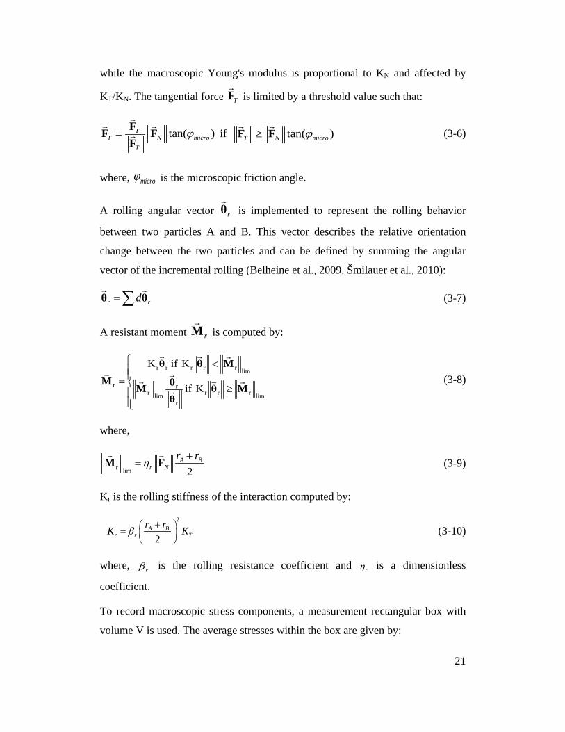
while the macroscopic Young's modulus is proportional to KN and affected by
KT/KN. The tangential force TF
is limited by a threshold value such that:
tan( )TT N micro
T
ϕ=FF FF
if tan( )T N microϕ≥F F
(3-6)
where, microϕ is the microscopic friction angle.
A rolling angular vector rθ
is implemented to represent the rolling behavior
between two particles A and B. This vector describes the relative orientation
change between the two particles and can be defined by summing the angular
vector of the incremental rolling (Belheine et al., 2009, Šmilauer et al., 2010):
r rd= ∑θ θ
(3-7)
A resistant moment rM
is computed by:
≥
<
=limrrr
r
rlimr
limrrrrr
r K if
K if K
MθθθM
Mθθ
M
(3-8)
where,
r lim 2A B
r Nr rη +
=M F
(3-9)
Kr is the rolling stiffness of the interaction computed by:
2
2A B
r r Tr rK Kβ + =
(3-10)
where, rβ is the rolling resistance coefficient and rη is a dimensionless
coefficient.
To record macroscopic stress components, a measurement rectangular box with
volume V is used. The average stresses within the box are given by:
21
, ,
1
1 cNc i c j
ijc
x fV
σ=
= ∑ (3-11)
where, cN is the number of contacts within the measurement box, jcf , is the
contact force vector at contact c, icx , is the branch vector connecting two contact
particles A and B, and indices i and j indicate the Cartesian coordinates.
Figure 3-1 a) An overview of the experimental setup; b) Model shaft during
assemblage and c) Lower-end section during assemblage (Adapted from Tobar,
2009)
Steel frame
Shaft model
Sand auger system
a)
Pre-calibrated handle
22
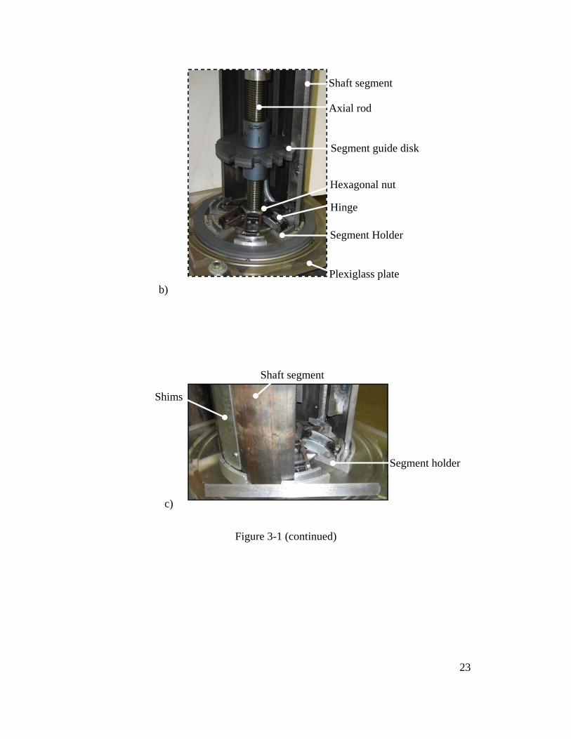
Figure 3-1 (continued)
Shims
Shaft segment
Segment holder
c))
Shaft segment
Plexiglass plate
Segment guide disk
Hinge
Segment Holder
b)
Hexagonal nut
Axial rod
23
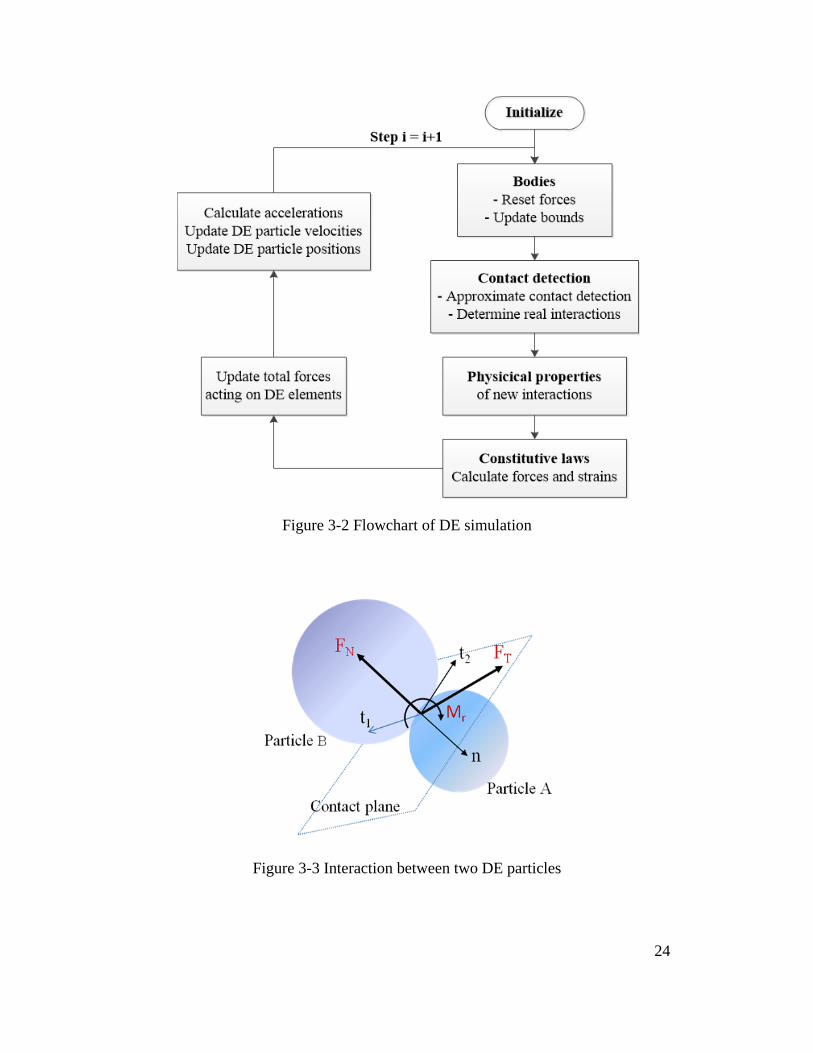
Figure 3-2 Flowchart of DE simulation
Figure 3-3 Interaction between two DE particles
24
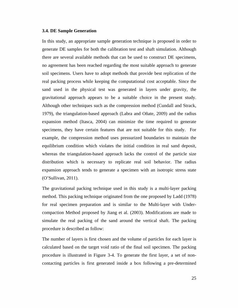
3.4. DE Sample Generation
In this study, an appropriate sample generation technique is proposed in order to
generate DE samples for both the calibration test and shaft simulation. Although
there are several available methods that can be used to construct DE specimens,
no agreement has been reached regarding the most suitable approach to generate
soil specimens. Users have to adopt methods that provide best replication of the
real packing process while keeping the computational cost acceptable. Since the
sand used in the physical test was generated in layers under gravity, the
gravitational approach appears to be a suitable choice in the present study.
Although other techniques such as the compression method (Cundall and Strack,
1979), the triangulation-based approach (Labra and Oñate, 2009) and the radius
expansion method (Itasca, 2004) can minimize the time required to generate
specimens, they have certain features that are not suitable for this study. For
example, the compression method uses pressurized boundaries to maintain the
equilibrium condition which violates the initial condition in real sand deposit,
whereas the triangulation-based approach lacks the control of the particle size
distribution which is necessary to replicate real soil behavior. The radius
expansion approach tends to generate a specimen with an isotropic stress state
(O’Sullivan, 2011).
The gravitational packing technique used in this study is a multi-layer packing
method. This packing technique originated from the one proposed by Ladd (1978)
for real specimen preparation and is similar to the Multi-layer with Under-
compaction Method proposed by Jiang et al. (2003). Modifications are made to
simulate the real packing of the sand around the vertical shaft. The packing
procedure is described as follow:
The number of layers is first chosen and the volume of particles for each layer is
calculated based on the target void ratio of the final soil specimen. The packing
procedure is illustrated in Figure 3-4. To generate the first layer, a set of non-
contacting particles is first generated inside a box following a pre-determined
25
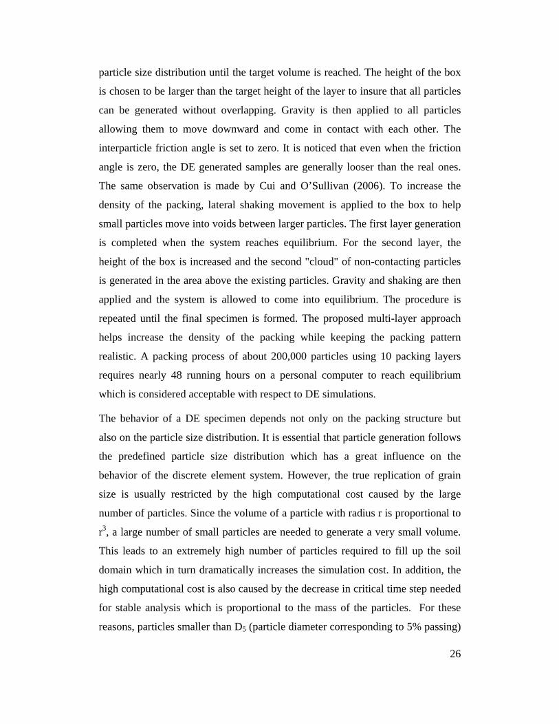
particle size distribution until the target volume is reached. The height of the box
is chosen to be larger than the target height of the layer to insure that all particles
can be generated without overlapping. Gravity is then applied to all particles
allowing them to move downward and come in contact with each other. The
interparticle friction angle is set to zero. It is noticed that even when the friction
angle is zero, the DE generated samples are generally looser than the real ones.
The same observation is made by Cui and O’Sullivan (2006). To increase the
density of the packing, lateral shaking movement is applied to the box to help
small particles move into voids between larger particles. The first layer generation
is completed when the system reaches equilibrium. For the second layer, the
height of the box is increased and the second "cloud" of non-contacting particles
is generated in the area above the existing particles. Gravity and shaking are then
applied and the system is allowed to come into equilibrium. The procedure is
repeated until the final specimen is formed. The proposed multi-layer approach
helps increase the density of the packing while keeping the packing pattern
realistic. A packing process of about 200,000 particles using 10 packing layers
requires nearly 48 running hours on a personal computer to reach equilibrium
which is considered acceptable with respect to DE simulations.
The behavior of a DE specimen depends not only on the packing structure but
also on the particle size distribution. It is essential that particle generation follows
the predefined particle size distribution which has a great influence on the
behavior of the discrete element system. However, the true replication of grain
size is usually restricted by the high computational cost caused by the large
number of particles. Since the volume of a particle with radius r is proportional to
r3, a large number of small particles are needed to generate a very small volume.
This leads to an extremely high number of particles required to fill up the soil
domain which in turn dramatically increases the simulation cost. In addition, the
high computational cost is also caused by the decrease in critical time step needed
for stable analysis which is proportional to the mass of the particles. For these
reasons, particles smaller than D5 (particle diameter corresponding to 5% passing)
26
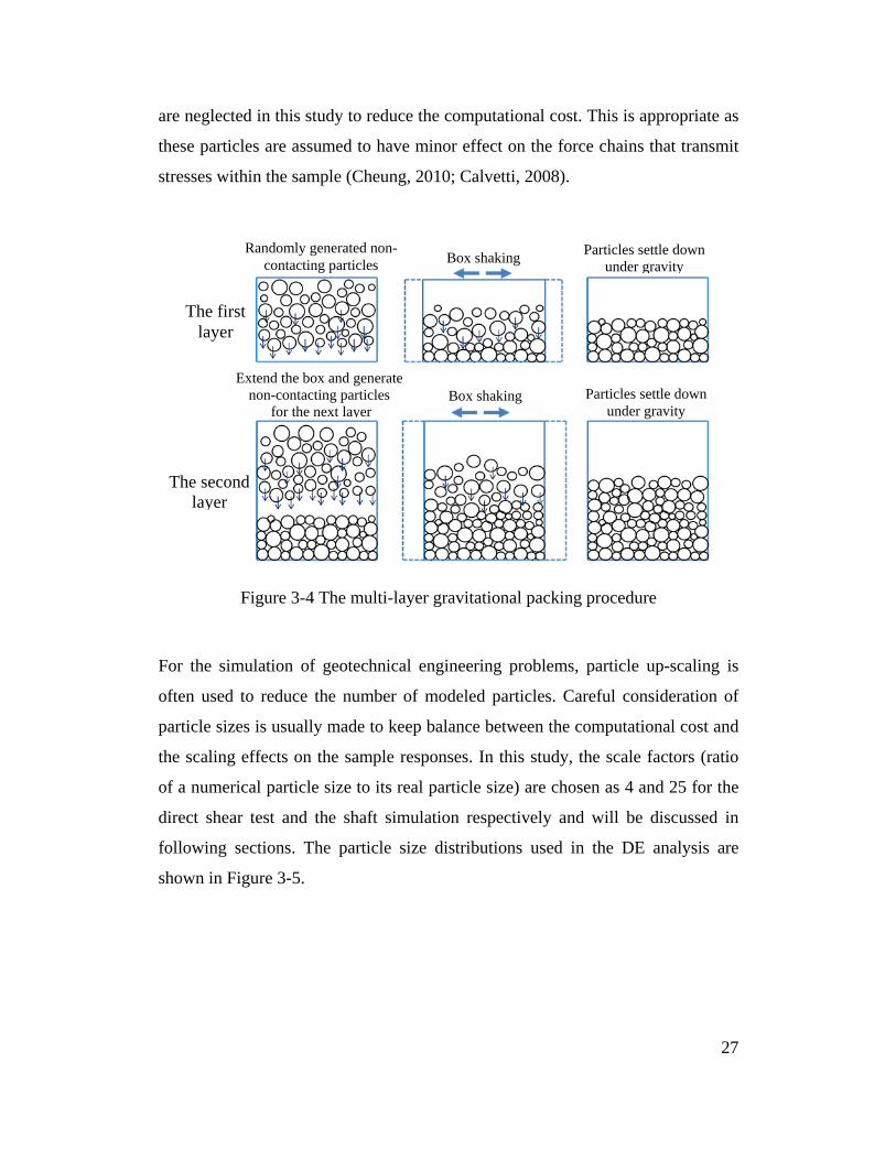
are neglected in this study to reduce the computational cost. This is appropriate as
these particles are assumed to have minor effect on the force chains that transmit
stresses within the sample (Cheung, 2010; Calvetti, 2008).
Figure 3-4 The multi-layer gravitational packing procedure
For the simulation of geotechnical engineering problems, particle up-scaling is
often used to reduce the number of modeled particles. Careful consideration of
particle sizes is usually made to keep balance between the computational cost and
the scaling effects on the sample responses. In this study, the scale factors (ratio
of a numerical particle size to its real particle size) are chosen as 4 and 25 for the
direct shear test and the shaft simulation respectively and will be discussed in
following sections. The particle size distributions used in the DE analysis are
shown in Figure 3-5.
The first layer
The second layer
Randomly generated non-contacting particles
Particles settle down under gravity
Extend the box and generate non-contacting particles
for the next layer
Particles settle down under gravity
Box shaking
Box shaking
27
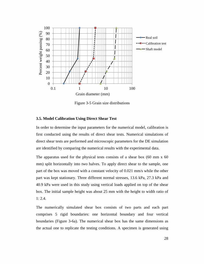
Figure 3-5 Grain size distributions
3.5. Model Calibration Using Direct Shear Test
In order to determine the input parameters for the numerical model, calibration is
first conducted using the results of direct shear tests. Numerical simulations of
direct shear tests are performed and microscopic parameters for the DE simulation
are identified by comparing the numerical results with the experimental data.
The apparatus used for the physical tests consists of a shear box (60 mm x 60
mm) split horizontally into two halves. To apply direct shear to the sample, one
part of the box was moved with a constant velocity of 0.021 mm/s while the other
part was kept stationary. Three different normal stresses, 13.6 kPa, 27.3 kPa and
40.9 kPa were used in this study using vertical loads applied on top of the shear
box. The initial sample height was about 25 mm with the height to width ratio of
1: 2.4.
The numerically simulated shear box consists of two parts and each part
comprises 5 rigid boundaries: one horizontal boundary and four vertical
boundaries (Figure 3-6a). The numerical shear box has the same dimensions as
the actual one to replicate the testing conditions. A specimen is generated using
0 10 20 30 40 50 60 70 80 90
100
0.1 1 10 100
Perc
ent w
eigh
t pas
sing
(%)
Grain diameter (mm)
Real soil
Calibration test
Shaft model
28
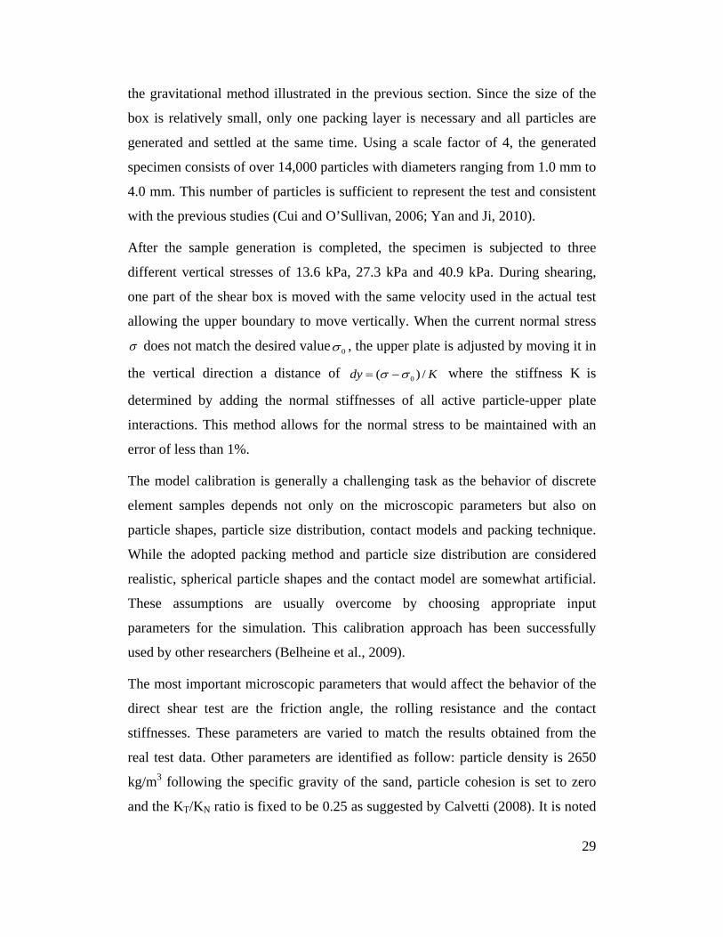
the gravitational method illustrated in the previous section. Since the size of the
box is relatively small, only one packing layer is necessary and all particles are
generated and settled at the same time. Using a scale factor of 4, the generated
specimen consists of over 14,000 particles with diameters ranging from 1.0 mm to
4.0 mm. This number of particles is sufficient to represent the test and consistent
with the previous studies (Cui and O’Sullivan, 2006; Yan and Ji, 2010).
After the sample generation is completed, the specimen is subjected to three
different vertical stresses of 13.6 kPa, 27.3 kPa and 40.9 kPa. During shearing,
one part of the shear box is moved with the same velocity used in the actual test
allowing the upper boundary to move vertically. When the current normal stress
σ does not match the desired value 0σ , the upper plate is adjusted by moving it in
the vertical direction a distance of 0( ) /dy Kσ σ= − where the stiffness K is
determined by adding the normal stiffnesses of all active particle-upper plate
interactions. This method allows for the normal stress to be maintained with an
error of less than 1%.
The model calibration is generally a challenging task as the behavior of discrete
element samples depends not only on the microscopic parameters but also on
particle shapes, particle size distribution, contact models and packing technique.
While the adopted packing method and particle size distribution are considered
realistic, spherical particle shapes and the contact model are somewhat artificial.
These assumptions are usually overcome by choosing appropriate input
parameters for the simulation. This calibration approach has been successfully
used by other researchers (Belheine et al., 2009).
The most important microscopic parameters that would affect the behavior of the
direct shear test are the friction angle, the rolling resistance and the contact
stiffnesses. These parameters are varied to match the results obtained from the
real test data. Other parameters are identified as follow: particle density is 2650
kg/m3 following the specific gravity of the sand, particle cohesion is set to zero
and the KT/KN ratio is fixed to be 0.25 as suggested by Calvetti (2008). It is noted
29
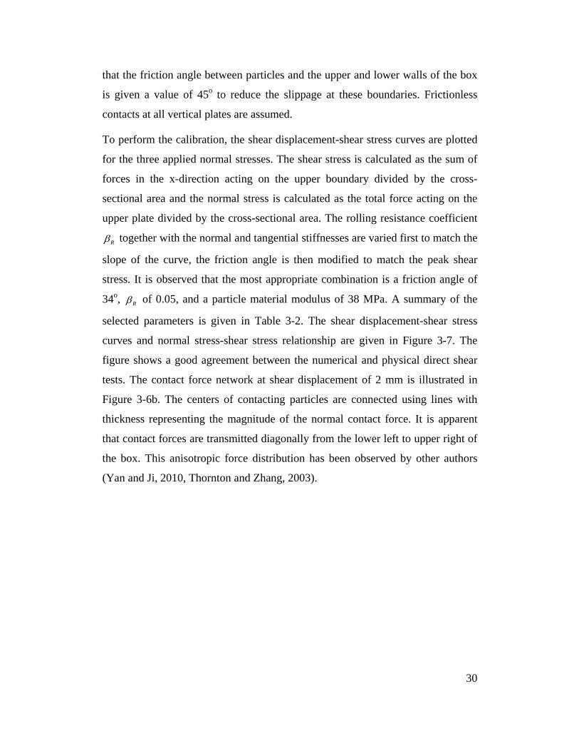
that the friction angle between particles and the upper and lower walls of the box
is given a value of 45o to reduce the slippage at these boundaries. Frictionless
contacts at all vertical plates are assumed.
To perform the calibration, the shear displacement-shear stress curves are plotted
for the three applied normal stresses. The shear stress is calculated as the sum of
forces in the x-direction acting on the upper boundary divided by the cross-
sectional area and the normal stress is calculated as the total force acting on the
upper plate divided by the cross-sectional area. The rolling resistance coefficient
Rβ together with the normal and tangential stiffnesses are varied first to match the
slope of the curve, the friction angle is then modified to match the peak shear
stress. It is observed that the most appropriate combination is a friction angle of
34o, Rβ of 0.05, and a particle material modulus of 38 MPa. A summary of the
selected parameters is given in Table 3-2. The shear displacement-shear stress
curves and normal stress-shear stress relationship are given in Figure 3-7. The
figure shows a good agreement between the numerical and physical direct shear
tests. The contact force network at shear displacement of 2 mm is illustrated in
Figure 3-6b. The centers of contacting particles are connected using lines with
thickness representing the magnitude of the normal contact force. It is apparent
that contact forces are transmitted diagonally from the lower left to upper right of
the box. This anisotropic force distribution has been observed by other authors
(Yan and Ji, 2010, Thornton and Zhang, 2003).
30
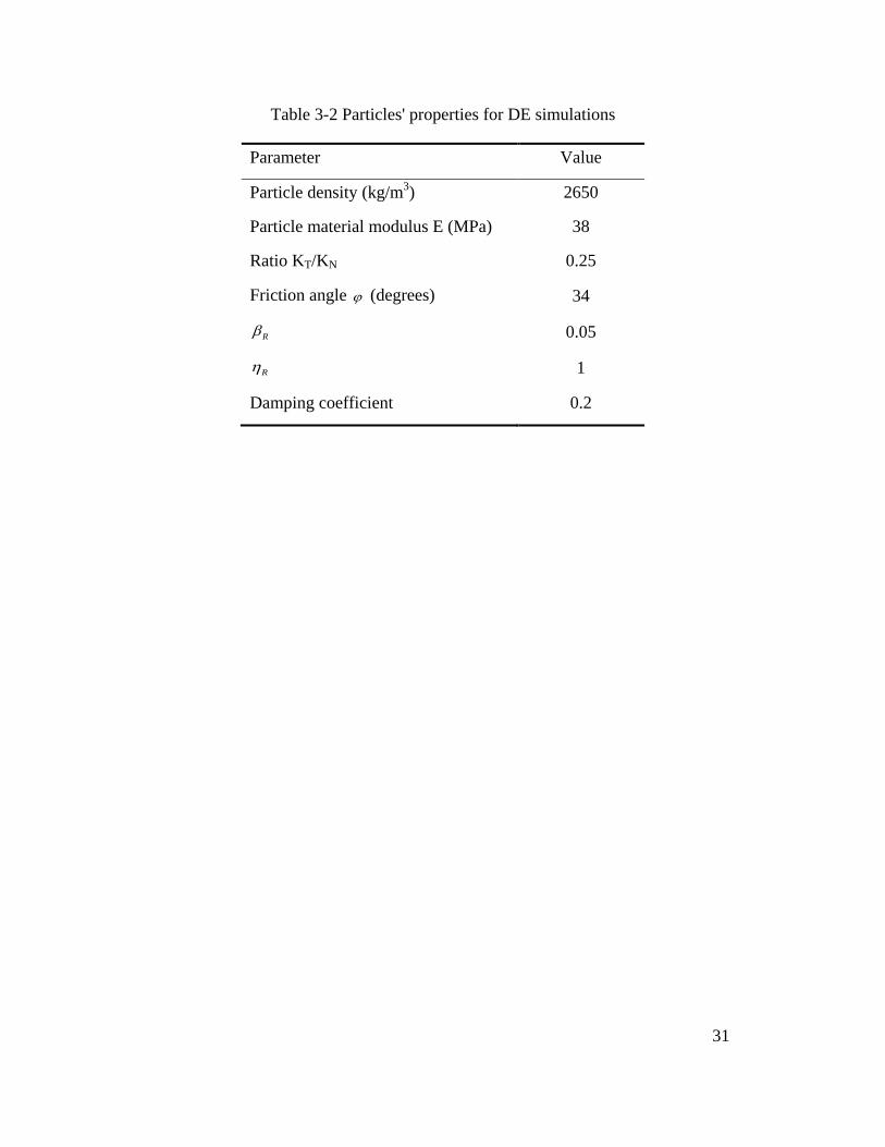
Table 3-2 Particles' properties for DE simulations
Parameter Value
Particle density (kg/m3) 2650
Particle material modulus E (MPa) 38
Ratio KT/KN 0.25
Friction angle ϕ (degrees) 34
Rβ 0.05
Rη 1
Damping coefficient 0.2
31

Figure 3-6 a) Three-dimensional direct shear sample and b) Three-dimensional
contact force network (at shear displacement of 2 m)
Direction of shearing
a)
b)
60 mm
60 mm
X
Z
Y
O
32
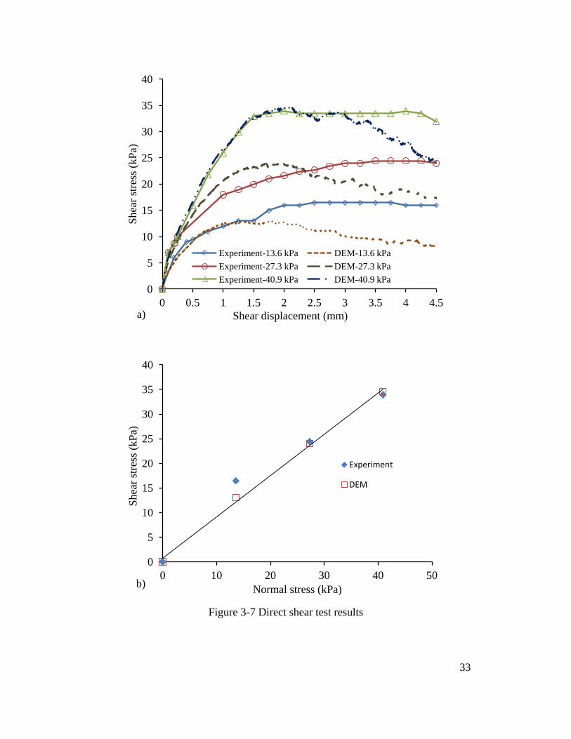
Figure 3-7 Direct shear test results
0
5
10
15
20
25
30
35
40
0 0.5 1 1.5 2 2.5 3 3.5 4 4.5
Shea
r stre
ss (k
Pa)
Shear displacement (mm)
Experiment-13.6 kPa DEM-13.6 kPa Experiment-27.3 kPa DEM-27.3 kPa Experiment-40.9 kPa DEM-40.9 kPa
a)
0
5
10
15
20
25
30
35
40
0 10 20 30 40 50
Shea
r stre
ss (k
Pa)
Normal stress (kPa)
Experiment
DEM
b)
33
3.6. Shaft-Soil Interaction Simulation
The vertical shaft is modeled using a cylinder 1.0 m in height and initial diameter
of 150 mm that comprises 12 equally distributed segments. Since the modeled
problem is axisymmetric, only part of the domain is modeled to reduce the
computational cost. In addition, better representation of the experiment can be
achieved by simulating one "slice" of the soil domain with a large number of
particles while keeping the simulation time acceptable. To capture the problem
geometry, a quarter of the problem is modeled in this study. The model consists of
a quarter of the shaft and four boundaries including three vertical and one
horizontal at the bottom of the container (Figure 3-8). Each quarter of the shaft is
divided into three segments to capture the curved shaft geometry. The friction
angles between particles and the wall boundaries are set to zero and pressures
acting on the shaft are recorded at the middle segment to reduce the boundary
effects. Similar technique has been used by Weatherley et al. (2011) to model
slope collapse and hopper flow problems.
The soil domain is generated using the proposed multi-layer packing technique
with 10 layers. In order to replicate the actual soil generation process, the friction
coefficient between the particles and the shaft is assumed to have a value of 0.2 to
account for the frictional contact between the shaft and the soil and is maintained
during the entire simulation. Using a scale factor of 25 and a total of over 245,000
particles are generated with diameters ranging from 6.25 mm to 25 mm. The
average void ratio of the generated soil sample is about 0.85 which is slightly
greater than the void ratio of the real sand (0.78). This is attributed to the removal
of excess sand to reach the target sample height.
The generated soil sample is checked to assure its equivalence (have the same
characteristics) to the soil specimen used in the direct shear test calibration. The
fabric tensor and coordination number are determined for the two samples at their
initial states. The fabric tensor is given by:
34
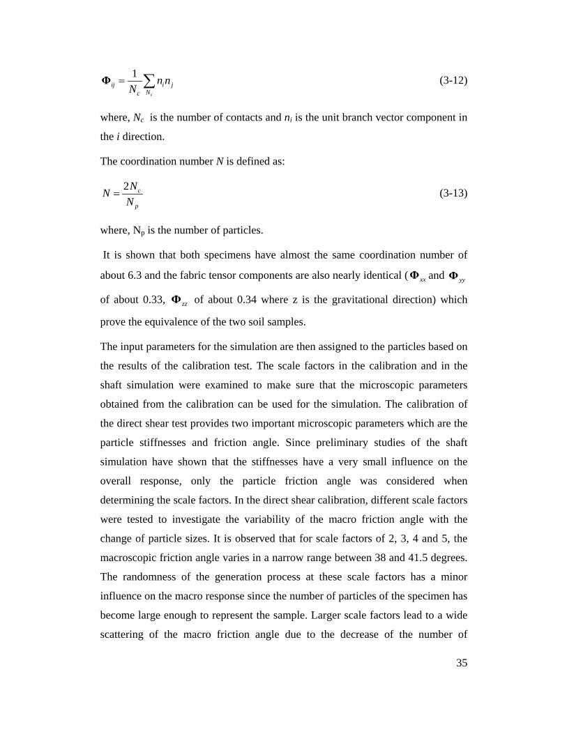
1
c
ij i jNc
n nN
= ∑Φ (3-12)
where, Nc is the number of contacts and ni is the unit branch vector component in
the i direction.
The coordination number N is defined as:
2 c
p
NNN
= (3-13)
where, Np is the number of particles.
It is shown that both specimens have almost the same coordination number of
about 6.3 and the fabric tensor components are also nearly identical ( xxΦ and yyΦ
of about 0.33, zzΦ of about 0.34 where z is the gravitational direction) which
prove the equivalence of the two soil samples.
The input parameters for the simulation are then assigned to the particles based on
the results of the calibration test. The scale factors in the calibration and in the
shaft simulation were examined to make sure that the microscopic parameters
obtained from the calibration can be used for the simulation. The calibration of
the direct shear test provides two important microscopic parameters which are the
particle stiffnesses and friction angle. Since preliminary studies of the shaft
simulation have shown that the stiffnesses have a very small influence on the
overall response, only the particle friction angle was considered when
determining the scale factors. In the direct shear calibration, different scale factors
were tested to investigate the variability of the macro friction angle with the
change of particle sizes. It is observed that for scale factors of 2, 3, 4 and 5, the
macroscopic friction angle varies in a narrow range between 38 and 41.5 degrees.
The randomness of the generation process at these scale factors has a minor
influence on the macro response since the number of particles of the specimen has
become large enough to represent the sample. Larger scale factors lead to a wide
scattering of the macro friction angle due to the decrease of the number of
35
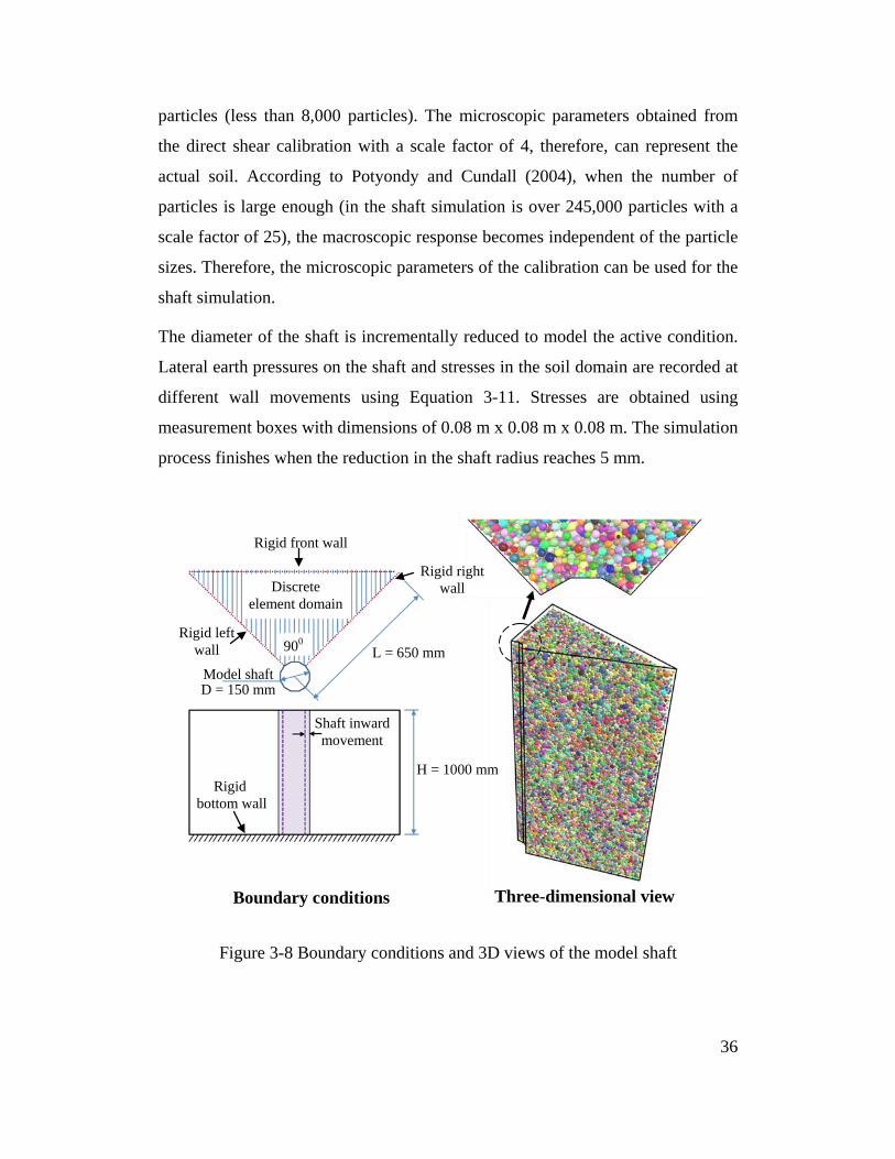
particles (less than 8,000 particles). The microscopic parameters obtained from
the direct shear calibration with a scale factor of 4, therefore, can represent the
actual soil. According to Potyondy and Cundall (2004), when the number of
particles is large enough (in the shaft simulation is over 245,000 particles with a
scale factor of 25), the macroscopic response becomes independent of the particle
sizes. Therefore, the microscopic parameters of the calibration can be used for the
shaft simulation.
The diameter of the shaft is incrementally reduced to model the active condition.
Lateral earth pressures on the shaft and stresses in the soil domain are recorded at
different wall movements using Equation 3-11. Stresses are obtained using
measurement boxes with dimensions of 0.08 m x 0.08 m x 0.08 m. The simulation
process finishes when the reduction in the shaft radius reaches 5 mm.
Figure 3-8 Boundary conditions and 3D views of the model shaft
Boundary conditions Three-dimensional view
Rigid bottom wall
Rigid right wall
Rigid left wall L = 650 mm
Discrete element domain
900
Model shaft D = 150 mm
Shaft inward movement
Rigid front wall
H = 1000 mm
36
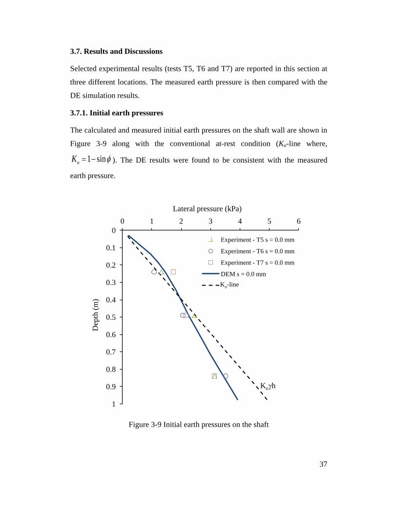
3.7. Results and Discussions
Selected experimental results (tests T5, T6 and T7) are reported in this section at
three different locations. The measured earth pressure is then compared with the
DE simulation results.
3.7.1. Initial earth pressures
The calculated and measured initial earth pressures on the shaft wall are shown in
Figure 3-9 along with the conventional at-rest condition (Ko-line where,
1 sinoK φ= − ). The DE results were found to be consistent with the measured
earth pressure.
Figure 3-9 Initial earth pressures on the shaft
0
0.1
0.2
0.3
0.4
0.5
0.6
0.7
0.8
0.9
1
0 1 2 3 4 5 6
Dep
th (m
)
Lateral pressure (kPa)
Experiment - T5 s = 0.0 mm
Experiment - T6 s = 0.0 mm
Experiment - T7 s = 0.0 mm
DEM s = 0.0 mm
KO- line Ko-line
Koγh
37
3.7.2. Earth pressure reduction with wall movement
Lateral pressures at different locations along the shaft are shown in Figure 3-10 to
3-13. The pressures are plotted versus the wall movement. Both the DE
simulation and the experimental results showed a consistent reduction in lateral
pressures as the wall movement increases. The earth pressure became independent
of the wall movement when the displacement reached about 3 mm. To study the
effects of the wall movement on the active earth pressure, the pressure, p, at a
certain depth is normalized with respect to the initial pressure, p0.
Normalized earth pressures at the three examined levels (0.24H, 0.49H and
0.84H) for different shaft wall movements are illustrated in Figure 3-14, 3-15 and
3-16, respectively. It can be seen that the DE results are in good agreement with
the experimental data. For a very small wall movement, a large reduction in
lateral earth pressure is observed. At a wall movement of 0.5 mm, the calculated
earth pressures decreased from 100% at the initial state to 55% at 0.24H and
0.49H and to 45% at 0.84H. For the same wall movement, the measured earth
pressures reached about 65% at 0.24H and 0.49H and about 50% at 0.84H. With
further increase in wall movement, the DE results were found to be identical to
the measured values. For movements between 1 mm and 2 mm, the earth pressure
decreased to 25% of the initial value at 0.24H and 0.49H and to 18% at 0.84H.
Additional movements larger than 3 mm did not cause significant pressure
reduction and the lateral pressures became constant when reached approximately
20% of the initial pressure at 0.24H and 0.49H and approximately 10% at 0.84H.
It can be concluded that the axisymmetric active earth pressure fully develops
when the shaft wall moves about 2 to 3 mm or about 2.5% to 4% of the shaft
radius. Furthermore, the most rapid reduction in the earth pressure is observed
near the bottom of the shaft.
38
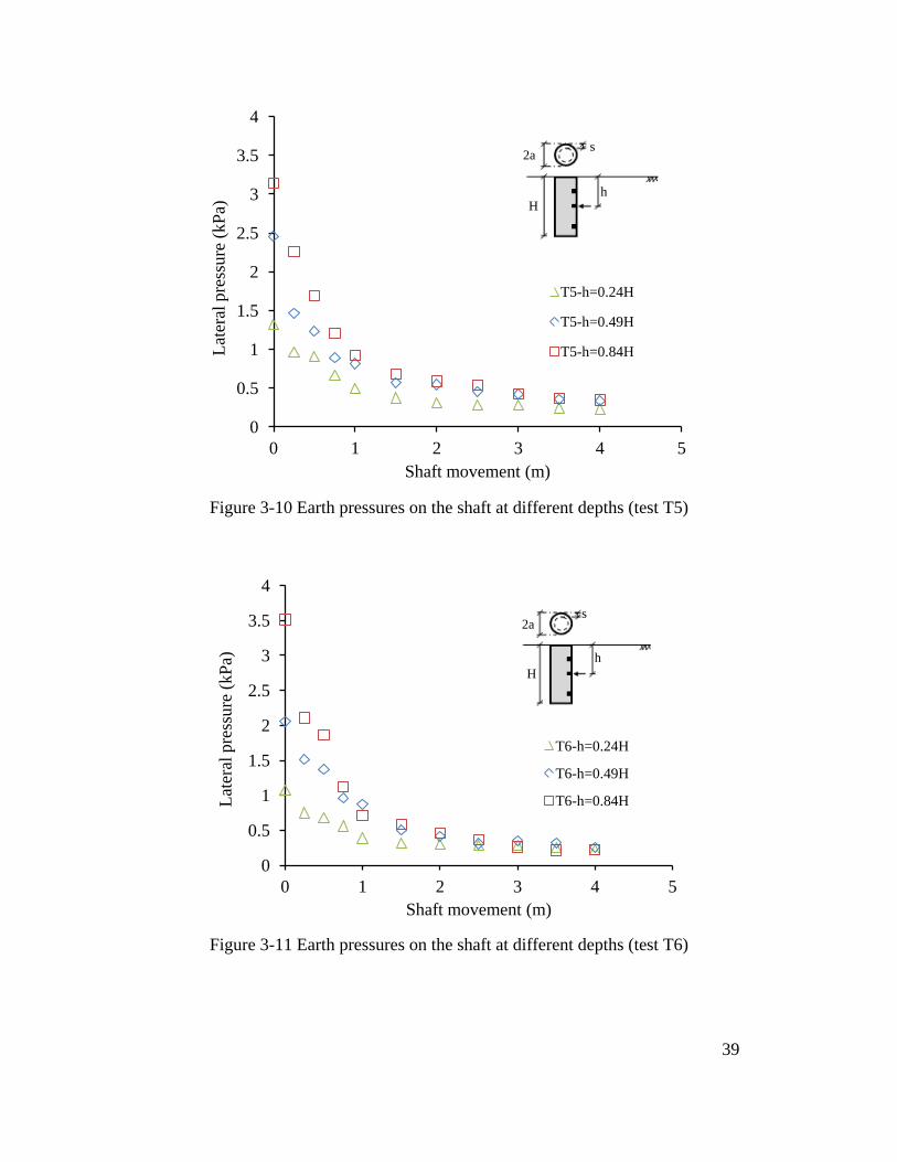
Figure 3-10 Earth pressures on the shaft at different depths (test T5)
Figure 3-11 Earth pressures on the shaft at different depths (test T6)
0
0.5
1
1.5
2
2.5
3
3.5
4
0 1 2 3 4 5
Late
ral p
ress
ure
(kPa
)
Shaft movement (m)
T5-h=0.24H
T5-h=0.49H
T5-h=0.84H
2a s
H h
0
0.5
1
1.5
2
2.5
3
3.5
4
0 1 2 3 4 5
Late
ral p
ress
ure
(kPa
)
Shaft movement (m)
T6-h=0.24H
T6-h=0.49H
T6-h=0.84H
2a
H h
s
39
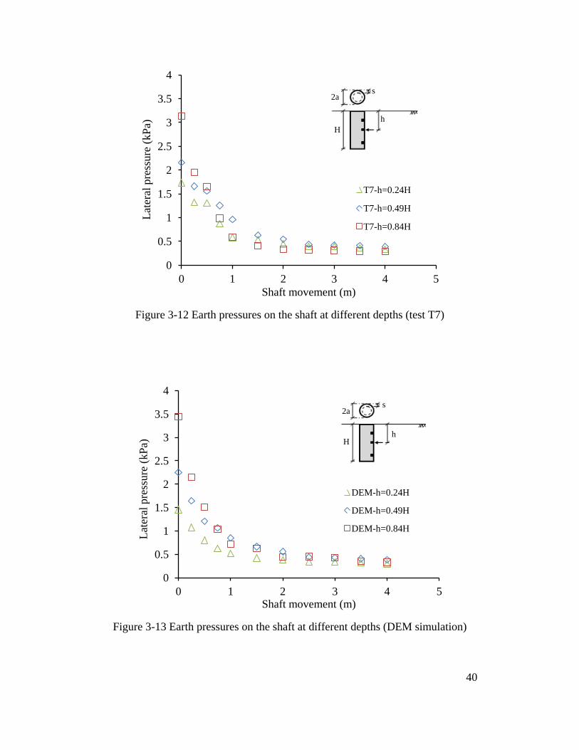
Figure 3-12 Earth pressures on the shaft at different depths (test T7)
Figure 3-13 Earth pressures on the shaft at different depths (DEM simulation)
0
0.5
1
1.5
2
2.5
3
3.5
4
0 1 2 3 4 5
Late
ral p
ress
ure
(kPa
)
Shaft movement (m)
T7-h=0.24H
T7-h=0.49H
T7-h=0.84H
2a s
H h
0
0.5
1
1.5
2
2.5
3
3.5
4
0 1 2 3 4 5
Late
ral p
ress
ure
(kPa
)
Shaft movement (m)
DEM-h=0.24H
DEM-h=0.49H
DEM-h=0.84H
2a s
H h
40
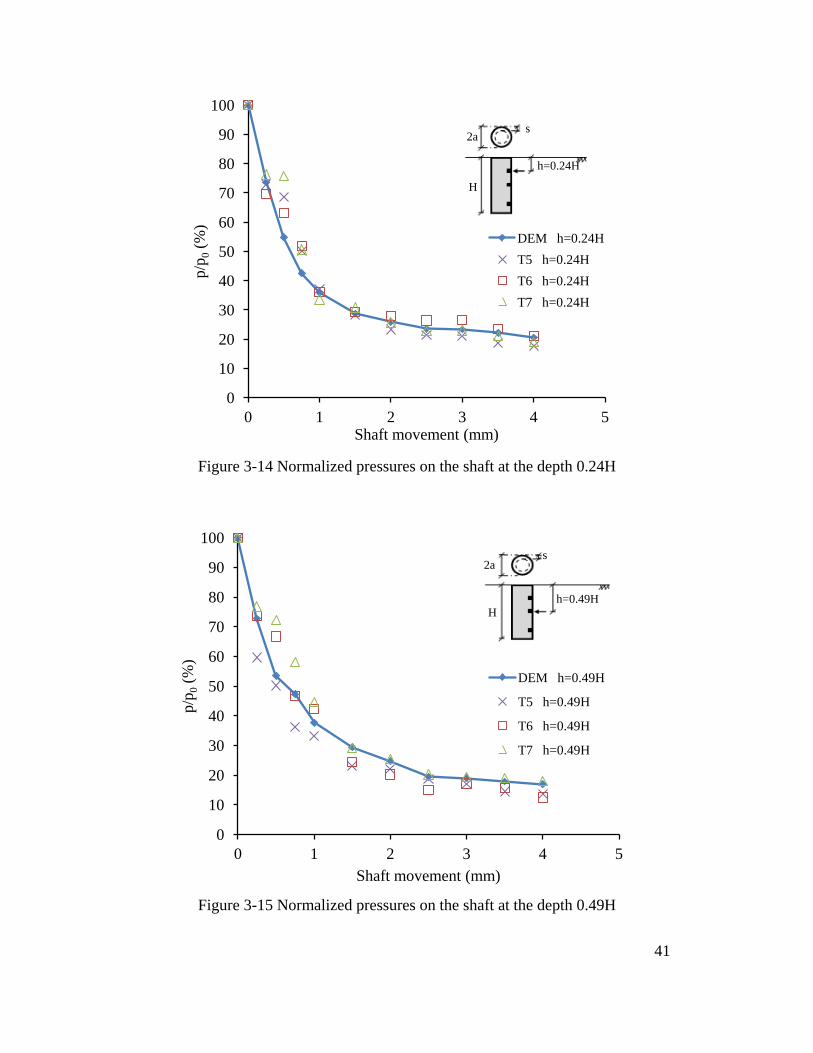
Figure 3-14 Normalized pressures on the shaft at the depth 0.24H
Figure 3-15 Normalized pressures on the shaft at the depth 0.49H
0
10
20
30
40
50
60
70
80
90
100
0 1 2 3 4 5
p/p 0
(%)
Shaft movement (mm)
DEM h=0.24H T5 h=0.24H T6 h=0.24H T7 h=0.24H
h=0.24H
H
2a s
0
10
20
30
40
50
60
70
80
90
100
0 1 2 3 4 5
p/p 0
(%)
Shaft movement (mm)
DEM h=0.49H
T5 h=0.49H
T6 h=0.49H
T7 h=0.49H
h=0.49H H
s 2a
41
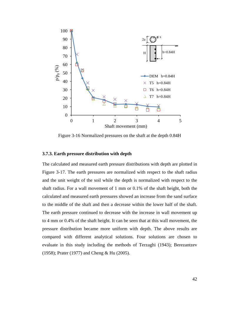
Figure 3-16 Normalized pressures on the shaft at the depth 0.84H
3.7.3. Earth pressure distribution with depth
The calculated and measured earth pressure distributions with depth are plotted in
Figure 3-17. The earth pressures are normalized with respect to the shaft radius
and the unit weight of the soil while the depth is normalized with respect to the
shaft radius. For a wall movement of 1 mm or 0.1% of the shaft height, both the
calculated and measured earth pressures showed an increase from the sand surface
to the middle of the shaft and then a decrease within the lower half of the shaft.
The earth pressure continued to decrease with the increase in wall movement up
to 4 mm or 0.4% of the shaft height. It can be seen that at this wall movement, the
pressure distribution became more uniform with depth. The above results are
compared with different analytical solutions. Four solutions are chosen to
evaluate in this study including the methods of Terzaghi (1943); Berezantzev
(1958); Prater (1977) and Cheng & Hu (2005).
0
10
20
30
40
50
60
70
80
90
100
0 1 2 3 4 5
p/p 0
(%)
Shaft movement (mm)
DEM h=0.84H
T5 h=0.84H
T6 h=0.84H
T7 h=0.84H
2a s
h=0.84H H
42
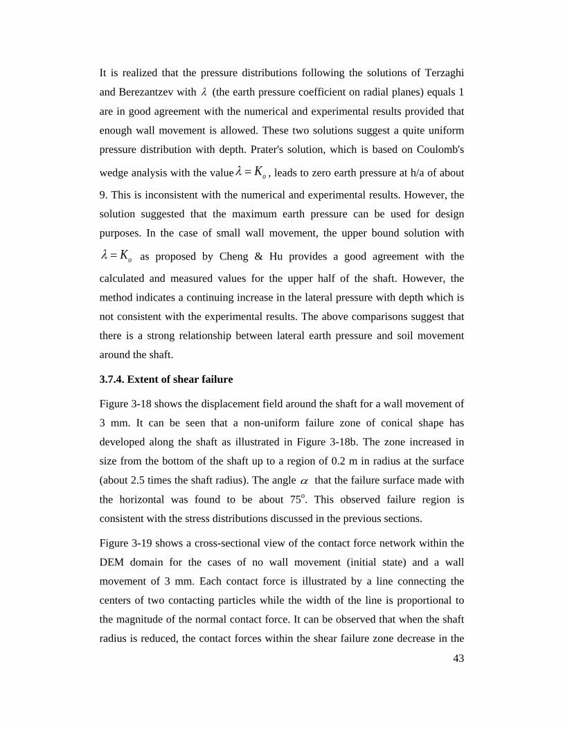
It is realized that the pressure distributions following the solutions of Terzaghi
and Berezantzev with λ (the earth pressure coefficient on radial planes) equals 1
are in good agreement with the numerical and experimental results provided that
enough wall movement is allowed. These two solutions suggest a quite uniform
pressure distribution with depth. Prater's solution, which is based on Coulomb's
wedge analysis with the value oKλ = , leads to zero earth pressure at h/a of about
9. This is inconsistent with the numerical and experimental results. However, the
solution suggested that the maximum earth pressure can be used for design
purposes. In the case of small wall movement, the upper bound solution with
oKλ = as proposed by Cheng & Hu provides a good agreement with the
calculated and measured values for the upper half of the shaft. However, the
method indicates a continuing increase in the lateral pressure with depth which is
not consistent with the experimental results. The above comparisons suggest that
there is a strong relationship between lateral earth pressure and soil movement
around the shaft.
3.7.4. Extent of shear failure
Figure 3-18 shows the displacement field around the shaft for a wall movement of
3 mm. It can be seen that a non-uniform failure zone of conical shape has
developed along the shaft as illustrated in Figure 3-18b. The zone increased in
size from the bottom of the shaft up to a region of 0.2 m in radius at the surface
(about 2.5 times the shaft radius). The angle α that the failure surface made with
the horizontal was found to be about 75o. This observed failure region is
consistent with the stress distributions discussed in the previous sections.
Figure 3-19 shows a cross-sectional view of the contact force network within the
DEM domain for the cases of no wall movement (initial state) and a wall
movement of 3 mm. Each contact force is illustrated by a line connecting the
centers of two contacting particles while the width of the line is proportional to
the magnitude of the normal contact force. It can be observed that when the shaft
radius is reduced, the contact forces within the shear failure zone decrease in the
43
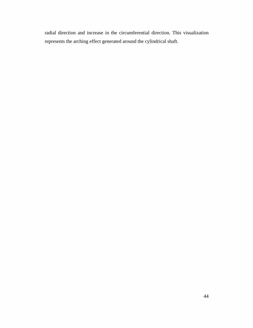
radial direction and increase in the circumferential direction. This visualization
represents the arching effect generated around the cylindrical shaft.
44
Figure 3-17 Comparison between modeled results and theoretical earth pressures
along the shaft. a) Shaft movement = 1 mm and b) Shaft movement = 4 mm
0
3
6
9
12
15 0 1 2 3
h / a
p / a· γ
T5
T6
T7
Terzaghi (1943)
Berezantzev (1958)
Prater (1977)
Cheng & Hu (2005)
DEM simulation
a)
λ=Ko
λ=1
λ=Ko
0
3
6
9
12
15 0 1 2 3
h / a
p / a· γ
T5
T6
T7
Terzaghi (1943)
Berezantzev (1958)
Prater (1977)
Cheng & Hu (2005)
DEM simulation
b)
λ=Ko
λ=1
λ=Ko
45
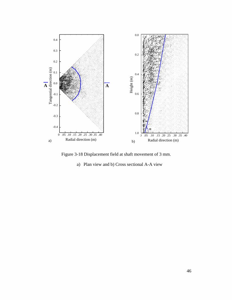
Figure 3-18 Displacement field at shaft movement of 3 mm.
a) Plan view and b) Cross sectional A-A view
Radial direction (m) 0 .05 .10 .15 .20 .25 .30 .35 .40 0 .05 .10 .15 .20 .25 .30 .35 .40
Radial direction (m)
0.0
0.2
0.4
0.6
0.8
1.0 H
eigh
t (m
)
0.4
0.3
0.2
0.1
0.0
-0.1
-0.2
-0.3
-0.4
Tang
entia
l dire
ctio
n (m
)
A A
a) b)
46
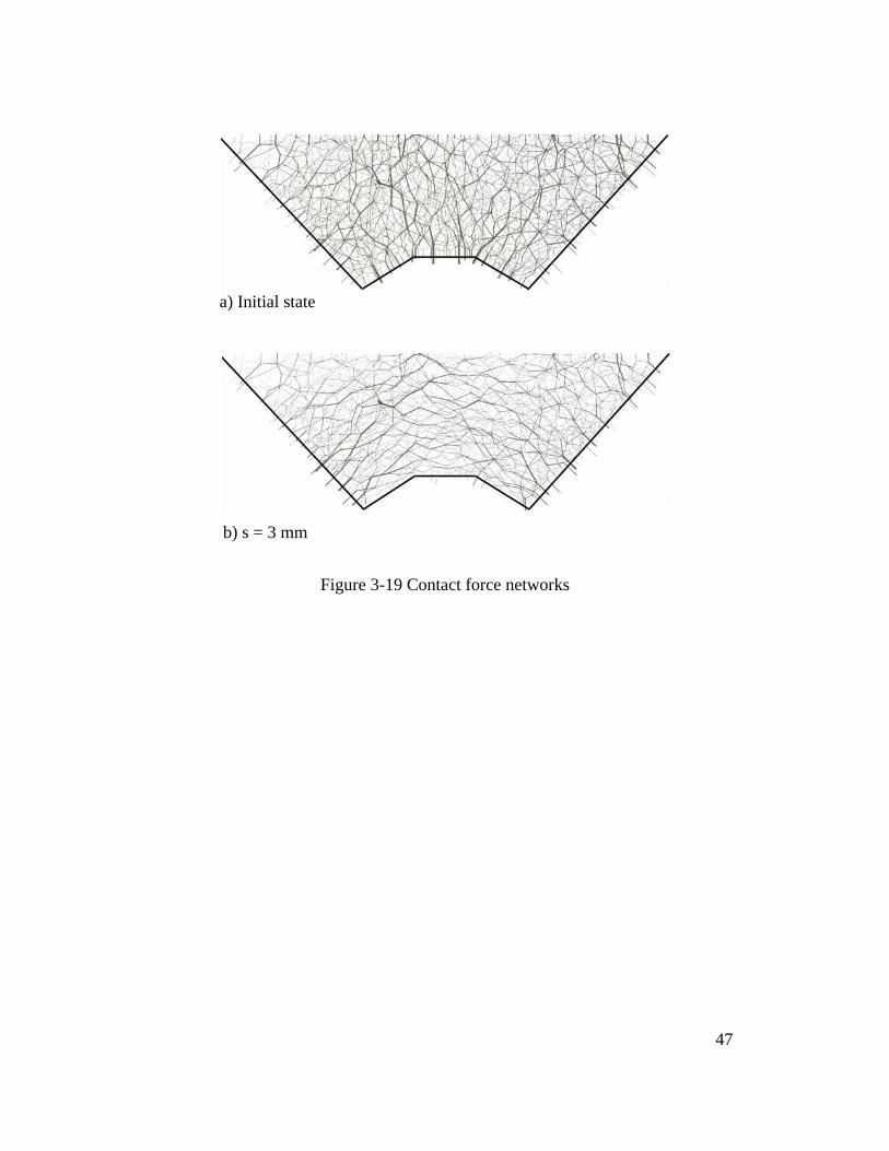
Figure 3-19 Contact force networks
a) Initial state
b) s = 3 mm
47

3.7.5. Stress distribution within the soil
Stresses within the soil mass including the radial, circumferential and vertical
components (see Figure 3-20) are analyzed at a chosen depth of 0.49H using the
DEM. The radial stress versus radial distance from the shaft centre is shown in
Figure 3-21. It can be seen in Figure 3-21a that radial stresses near the shaft wall
dropped rapidly even for a small wall movement of 1 mm. Increase in wall
movements from 2 mm to 3 mm caused the radial stress to further decrease.
However, no significant change in radial stress was observed for movements
larger than 3 mm. The radial stress in the vicinity of the shaft remained at about
60% of the initial value for wall movement of 1 mm and about 40% for wall
movement of 3 mm. The distribution of the radial stress in a cross section is
shown in Figure 3-21b. It was found that the changes in radial stress mostly
occurred within 0.3 m from the center of the shaft. The stresses outside this region
remained close to its initial state despite the wall movement.
Figure 3-20 Stresses acting on a soil element
r
z
Radial stress σr
Vertical stress σz
τzr
τrz σθ Circumferential stress
48
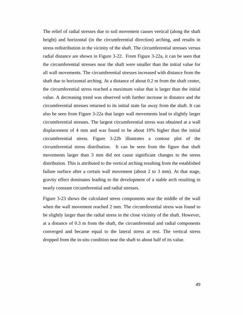
The relief of radial stresses due to soil movement causes vertical (along the shaft
height) and horizontal (in the circumferential direction) arching, and results in
stress redistribution in the vicinity of the shaft. The circumferential stresses versus
radial distance are shown in Figure 3-22. From Figure 3-22a, it can be seen that
the circumferential stresses near the shaft were smaller than the initial value for
all wall movements. The circumferential stresses increased with distance from the
shaft due to horizontal arching. At a distance of about 0.2 m from the shaft center,
the circumferential stress reached a maximum value that is larger than the initial
value. A decreasing trend was observed with further increase in distance and the
circumferential stresses returned to its initial state far away from the shaft. It can
also be seen from Figure 3-22a that larger wall movements lead to slightly larger
circumferential stresses. The largest circumferential stress was obtained at a wall
displacement of 4 mm and was found to be about 10% higher than the initial
circumferential stress. Figure 3-22b illustrates a contour plot of the
circumferential stress distribution. It can be seen from the figure that shaft
movements larger than 3 mm did not cause significant changes to the stress
distribution. This is attributed to the vertical arching resulting from the established
failure surface after a certain wall movement (about 2 to 3 mm). At that stage,
gravity effect dominates leading to the development of a stable arch resulting in
nearly constant circumferential and radial stresses.
Figure 3-23 shows the calculated stress components near the middle of the wall
when the wall movement reached 2 mm. The circumferential stress was found to
be slightly larger than the radial stress in the close vicinity of the shaft. However,
at a distance of 0.3 m from the shaft, the circumferential and radial components
converged and became equal to the lateral stress at rest. The vertical stress
dropped from the in-situ condition near the shaft to about half of its value.
49
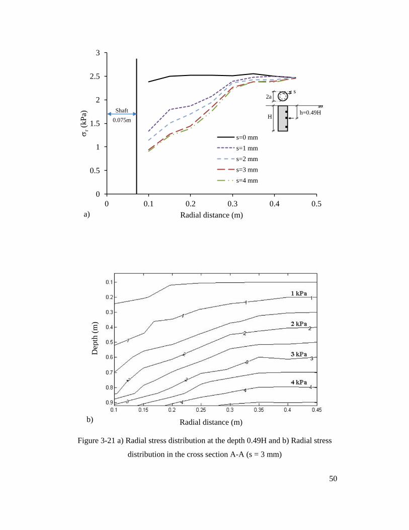
Figure 3-21 a) Radial stress distribution at the depth 0.49H and b) Radial stress
distribution in the cross section A-A (s = 3 mm)
0
0.5
1
1.5
2
2.5
3
0 0.1 0.2 0.3 0.4 0.5
σ r (k
Pa)
Radial distance (m)
s=0 mm s=1 mm s=2 mm s=3 mm s=4 mm
s 2a
H h=0.49H Shaft
0.075m
a)
b) Radial distance (m)
Dep
th (m
)
50
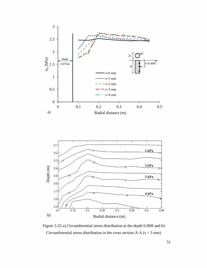
Figure 3-22 a) Circumferential stress distribution at the depth 0.49H and b)
Circumferential stress distribution in the cross section A-A (s = 3 mm)
0
0.5
1
1.5
2
2.5
3
0 0.1 0.2 0.3 0.4 0.5
σ θ (k
Pa)
Radial distance (m)
s=0 mm s=1 mm s=2 mm s=3 mm s=4 mm
s 2a
H h=0.49H
Shaft 0.075m
a)
b) Radial distance (m)
Dep
th (m
)
51
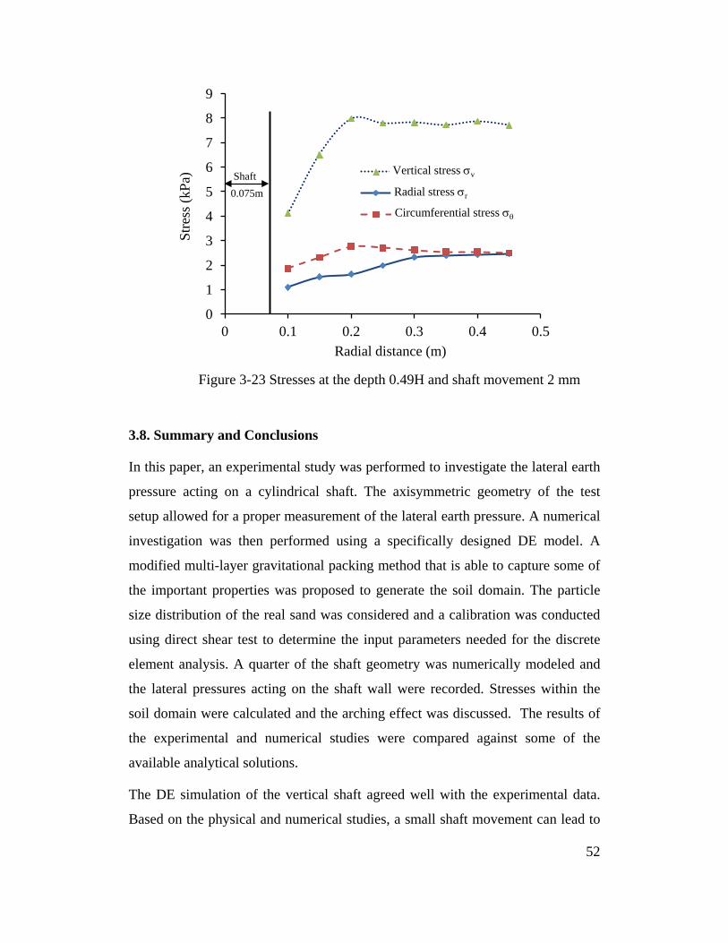
Figure 3-23 Stresses at the depth 0.49H and shaft movement 2 mm
3.8. Summary and Conclusions
In this paper, an experimental study was performed to investigate the lateral earth
pressure acting on a cylindrical shaft. The axisymmetric geometry of the test
setup allowed for a proper measurement of the lateral earth pressure. A numerical
investigation was then performed using a specifically designed DE model. A
modified multi-layer gravitational packing method that is able to capture some of
the important properties was proposed to generate the soil domain. The particle
size distribution of the real sand was considered and a calibration was conducted
using direct shear test to determine the input parameters needed for the discrete
element analysis. A quarter of the shaft geometry was numerically modeled and
the lateral pressures acting on the shaft wall were recorded. Stresses within the
soil domain were calculated and the arching effect was discussed. The results of
the experimental and numerical studies were compared against some of the
available analytical solutions.
The DE simulation of the vertical shaft agreed well with the experimental data.
Based on the physical and numerical studies, a small shaft movement can lead to
0
1
2
3
4
5
6
7
8
9
0 0.1 0.2 0.3 0.4 0.5
Stre
ss (k
Pa)
Radial distance (m)
sigma_V
Sigma_R
Sigma_T
Shaft 0.075m
Vertical stress σv
Radial stress σr
Circumferential stress σθ
52
a rapid decrease in the earth pressure acting on the shaft wall. The required shaft
movement to reach the full active condition was found to range from 2.5% to 4%
of the shaft radius or 0.2% to 0.3% of the shaft height. At this wall movement, the
earth pressure can significantly decrease to a value of 10% of the initial pressure
and the lateral pressure becomes uniform with depth. The analytical solutions of
Terzaghi and Berezantzev were found to be in good agreement with the observed
pressure distribution.
The movement of the shaft wall resulted in stress redistribution within the soil
medium. The arching effect has lead to a decrease in radial stresses and increase
in circumferential stresses within a region of radius 0.3 m from the shaft center.
The stresses in the soil domain became quite stable when the wall movement
reached 3 mm. The agreement between the numerical and measured results
demonstrated the efficiency of the DEM in validating geotechnical problems
involving granular material and large deformation.
53
Preface to Chapter 4
The results presented in the previous chapter demonstrate the efficiency of the
discrete element method in investigating the behavior of granular material. In
these analyses, the soil particles were modeled using spherical particles whereas
the wall was modeled as a rigid boundary. Therefore, the response of the wall was
not investigated. In problems involving soil-structure interaction, it is challenging
to simultaneously model both the 3D discontinuous nature of the soil and the
continuous nature of the structural elements using traditional discrete or finite
element method. The coupling of the finite and discrete element methods allows
for the simulation of such problems. In this chapter, a coupled Finite-Discrete
framework is presented and then used to investigate the behavior of a biaxial
geogrid sheet embedded in sand material subjected to pullout loading.
54
CHAPTER 4
Three-Dimensional Modeling of Geogrid-Soil Interaction under Pullout Loading Conditions *
Abstract
The behavior of a geogrid-soil system is dependent on the properties of the
geogrid material, the backfill soil and the interface condition. Modeling the
geogrid-soil interaction taking into account the true geogrid geometry is a
challenging numerical problem that requires the consideration of the
discontinuous nature of the soil and the different modes of resistance that
contribute to the pullout capacity of the geogrid layer. In this study, a coupled
Finite-Discrete framework has been developed to investigate the behavior of a
biaxial geogrid sheet embedded in granular material and subjected to pullout
loading. Validation is performed by comparing experimental data and numerically
calculated results using the proposed model. The detailed behavior of the geogrid
and the surrounding soil is then investigated. The numerical results indicated the
suitability of the coupled model to solve this class of problems.
Keywords: soil reinforcement, biaxial geogrid, pullout loading, finite-discrete
element.
* A version of this chapter has been published in Geotextiles and Geomembranes,
2013, 37: 1-9.
55
4.1. Introduction
Geosynthetics are extensively used in civil engineering practice to facilitate cost
effective building, environmental, transportation and other construction projects.
A geogrid is geosynthetic material used to reinforce soils and improve the overall
performance of foundations, roadways, walls and slopes. In the past two decades,
both theoretical and experimental studies have been used to investigate the
mechanics of reinforced soil systems under pullout loading condition (Farrag et
al., 1993; Bergado and Chai, 1994; Ochiai et al., 1996; Sugimoto et. al., 2001;
Palmeira, 2004; Moraci and Recalcati, 2006; Sieira et al., 2009). While it possible
to track the load-displacement response of geogrid in pullout experiments, the
behavior of the backfill soil as it interacts with the geogrid material is hard to
evaluate experimentally and numerical methods are considered more suitable for
that purpose.
Finite element method (FEM) is widely used as a numerical tool to model the soil
reinforcement pullout procedure (Sugimoto and Alagiyawanna, 2003; Khedkar
and Mandal, 2009). The geogrid geometry is often simplified either as a truss
structure (in 2D analysis) or a continuous sheet (in 3D analysis). Using this
approach makes it difficult to separate the contributions of the frictional and
bearing resistances with respect to the overall pullout capacity of a reinforced
system. In addition, it makes it also challenging to determine the stress and strain
distributions in the geogrid members as well as in the surrounding soil material.
As an alternative to the continuum approach, the discrete element method (DEM)
has been used by several researchers to model the soil-geogrid interaction.
McDowell et al. (2006) and Chen et al. (2012) used DE method to model both the
geogrid and the backfill soil. In this approach, the geogrid is modeled using a set
of spherical particles bonded together to form the geogrid shape. The interaction
between the geogrid and the surrounding soil is obtained through the contact
between discrete particles. Although microscopic parameters of the geogrid
bonded particles are determined using some index load tests, the complex geogrid
56
deformation during the actual test may not be accurately captured due to the
inflexibility of the bonded particles. Moreover, since a set of bonded discrete
particles can roughly capture the geogrid continuous nature, the accuracy of the
strains and stresses within the geogrid layer may not be obtained.
To take advantage of both the FE and DE methods, the reinforcement layer can be
modeled using FE whereas the backfill soil can be modeled using DE method.
The coupling of the two methods can efficiently model the behavior of the
geogrid as well as the backfill soil material. This approach has been used by
several researchers to solve certain problems such as: geosynthetic-reinforced
earth structures (Villard et al., 2009), pile installation (Elmekati and Shamy,
2010) and earth pressure on tunnel linings (Dang and Meguid, 2011). In this
paper, a coupled Finite-Discrete element (FE-DE) framework is presented.
Geogrid pullout tests based on laboratory experiments are modeled using the
developed framework. The results of the numerical simulation including the
detailed response of the geogrid and the surrounding soil are presented and
compared with experimental data. Although emphasis is placed in this study on
the frictional and bearing components of the pullout resistance, displacements,
stresses, and strain fields in the vicinity of the geogrid layer are also highlighted.
4.2. Coupled Finite-Discrete Element Framework
The coupled FE-DE framework used in this study is a continuation of the original
work of Dang and Meguid (2010, 2013). The developed algorithm is implemented
into an open source discrete element code YADE (Kozicki and Donze, 2009;
Šmilauer et al., 2010) and is briefly described in the following sections.
4.2.1. Discrete Elements
The contact law between particles used in the framework is briefly described
below:
57
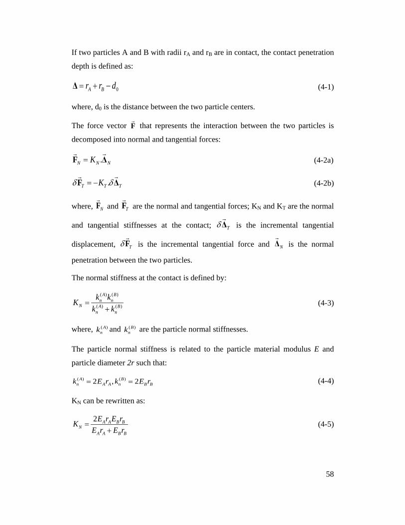
If two particles A and B with radii rA and rB are in contact, the contact penetration
depth is defined as:
0A Br r d= + −Δ (4-1)
where, d0 is the distance between the two particle centers.
The force vector F
that represents the interaction between the two particles is
decomposed into normal and tangential forces:
.N N NK=F Δ
(4-2a)
.T T TKδ δ= −F Δ
(4-2b)
where, NF
and TF
are the normal and tangential forces; KN and KT are the normal
and tangential stiffnesses at the contact; TδΔ
is the incremental tangential
displacement, Tδ F
is the incremental tangential force and NΔ
is the normal
penetration between the two particles.
The normal stiffness at the contact is defined by:
( ) ( )
( ) ( )
A Bn n
N A Bn n
k kKk k
=+
(4-3)
where, ( )Ank and ( )B
nk are the particle normal stiffnesses.
The particle normal stiffness is related to the particle material modulus E and
particle diameter 2r such that:
( ) ( )2 , 2A Bn A A n B Bk E r k E r= = (4-4)
KN can be rewritten as:
2 A A B BN
A A B B
E r E rKE r E r
=+
(4-5)
58
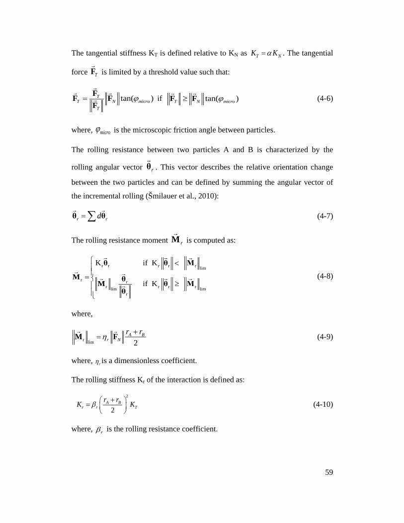
The tangential stiffness KT is defined relative to KN as T NK Kα= . The tangential
force TF
is limited by a threshold value such that:
tan( )TT N micro
T
ϕ=FF FF
if tan( )T N microϕ≥F F
(4-6)
where, microϕ is the microscopic friction angle between particles.
The rolling resistance between two particles A and B is characterized by the
rolling angular vector rθ
. This vector describes the relative orientation change
between the two particles and can be defined by summing the angular vector of
the incremental rolling (Šmilauer et al., 2010):
r rd= ∑θ θ
(4-7)
The rolling resistance moment rM
is computed as:
r r r r r lim
r rr r r rlim lim
r
K if K
if K
<=
≥
θ θ M
M θM θ Mθ
(4-8)
where,
r lim 2A B
r Nr rη +
=M F
(4-9)
where, rη is a dimensionless coefficient.
The rolling stiffness Kr of the interaction is defined as:
2
2A B
r r Tr rK Kβ + =
(4-10)
where, rβ is the rolling resistance coefficient.
59
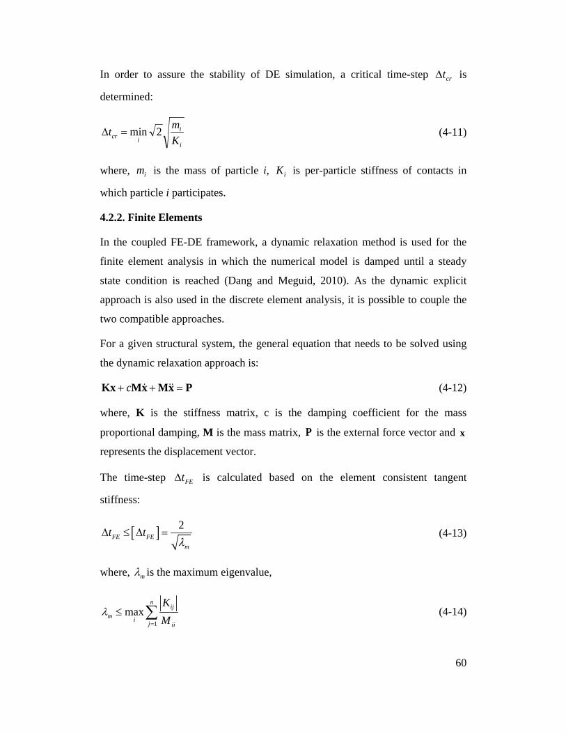
In order to assure the stability of DE simulation, a critical time-step crt∆ is
determined:
i
iicr K
mt 2min=∆ (4-11)
where, im is the mass of particle i, iK is per-particle stiffness of contacts in
which particle i participates.
4.2.2. Finite Elements
In the coupled FE-DE framework, a dynamic relaxation method is used for the
finite element analysis in which the numerical model is damped until a steady
state condition is reached (Dang and Meguid, 2010). As the dynamic explicit
approach is also used in the discrete element analysis, it is possible to couple the
two compatible approaches.
For a given structural system, the general equation that needs to be solved using
the dynamic relaxation approach is:
PxMxMKx =++ c (4-12)
where, K is the stiffness matrix, c is the damping coefficient for the mass
proportional damping, M is the mass matrix, P is the external force vector and x
represents the displacement vector.
The time-step FEt∆ is calculated based on the element consistent tangent
stiffness:
[ ] 2FE FE
m
t tλ
∆ ≤ ∆ = (4-13)
where, mλ is the maximum eigenvalue,
1max
nij
m i j ii
KM
λ=
≤ ∑ (4-14)
60
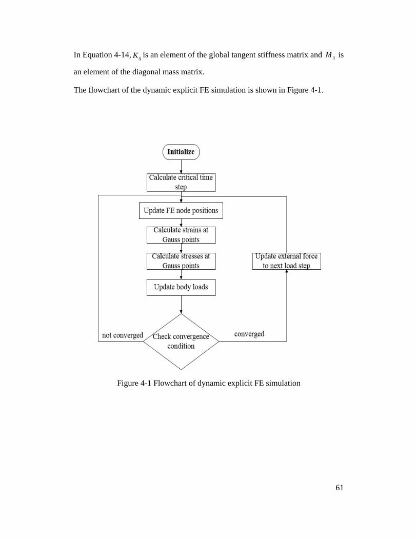
In Equation 4-14, ijK is an element of the global tangent stiffness matrix and iiM is
an element of the diagonal mass matrix.
The flowchart of the dynamic explicit FE simulation is shown in Figure 4-1.
Figure 4-1 Flowchart of dynamic explicit FE simulation
61
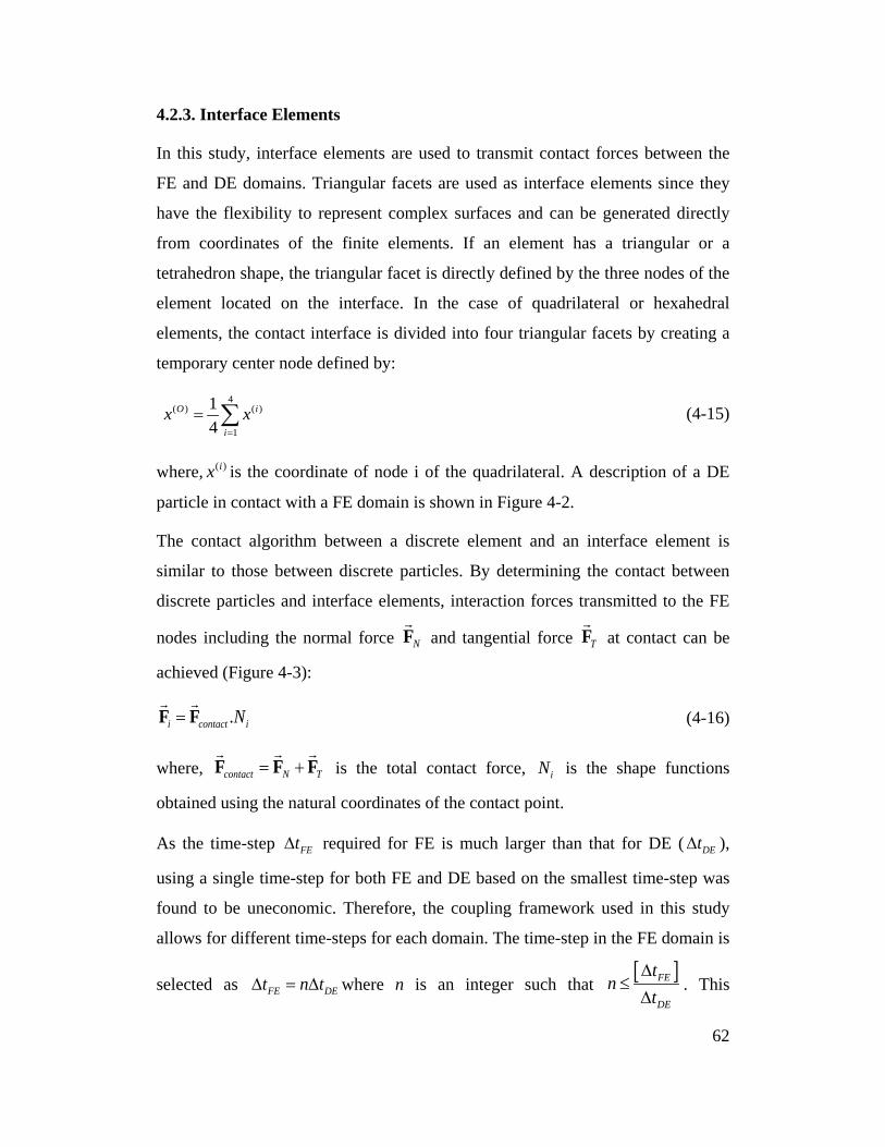
4.2.3. Interface Elements
In this study, interface elements are used to transmit contact forces between the
FE and DE domains. Triangular facets are used as interface elements since they
have the flexibility to represent complex surfaces and can be generated directly
from coordinates of the finite elements. If an element has a triangular or a
tetrahedron shape, the triangular facet is directly defined by the three nodes of the
element located on the interface. In the case of quadrilateral or hexahedral
elements, the contact interface is divided into four triangular facets by creating a
temporary center node defined by:
4
( ) ( )
1
14
O i
ix x
=
= ∑ (4-15)
where, ( )ix is the coordinate of node i of the quadrilateral. A description of a DE
particle in contact with a FE domain is shown in Figure 4-2.
The contact algorithm between a discrete element and an interface element is
similar to those between discrete particles. By determining the contact between
discrete particles and interface elements, interaction forces transmitted to the FE
nodes including the normal force NF
and tangential force TF
at contact can be
achieved (Figure 4-3):
.i contact iN=F F
(4-16)
where, contact N T= +F F F
is the total contact force, iN is the shape functions
obtained using the natural coordinates of the contact point.
As the time-step FEt∆ required for FE is much larger than that for DE ( DEt∆ ),
using a single time-step for both FE and DE based on the smallest time-step was
found to be uneconomic. Therefore, the coupling framework used in this study
allows for different time-steps for each domain. The time-step in the FE domain is
selected as FE DEt n t∆ = ∆ where n is an integer such that [ ]FE
DE
tn
t∆
≤∆
. This
62
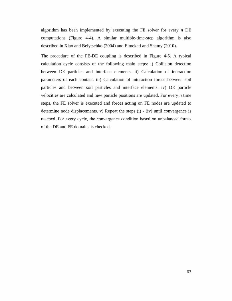
algorithm has been implemented by executing the FE solver for every n DE
computations (Figure 4-4). A similar multiple-time-step algorithm is also
described in Xiao and Belytschko (2004) and Elmekati and Shamy (2010).
The procedure of the FE-DE coupling is described in Figure 4-5. A typical
calculation cycle consists of the following main steps: i) Collision detection
between DE particles and interface elements. ii) Calculation of interaction
parameters of each contact. iii) Calculation of interaction forces between soil
particles and between soil particles and interface elements. iv) DE particle
velocities are calculated and new particle positions are updated. For every n time
steps, the FE solver is executed and forces acting on FE nodes are updated to
determine node displacements. v) Repeat the steps (i) - (iv) until convergence is
reached. For every cycle, the convergence condition based on unbalanced forces
of the DE and FE domains is checked.
63
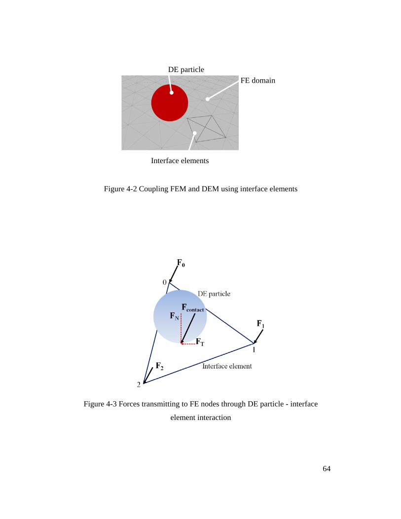
Figure 4-2 Coupling FEM and DEM using interface elements
Figure 4-3 Forces transmitting to FE nodes through DE particle - interface
element interaction
Interface elements
DE particle FE domain
64
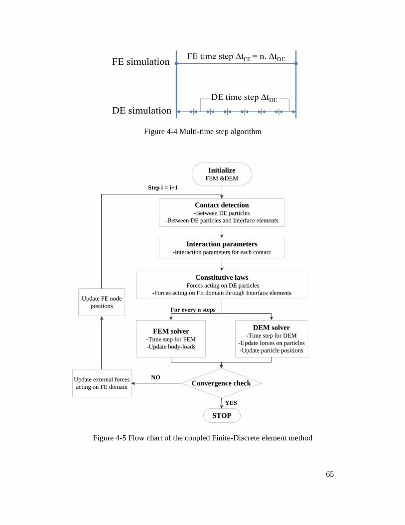
Figure 4-4 Multi-time step algorithm
InitializeFEM &DEMInitialize
FEM &DEM
Contact detection-Between DE particles
-Between DE particles and Interface elements
Contact detection-Between DE particles
-Between DE particles and Interface elements
Constitutive laws-Forces acting on DE particles
-Forces acting on FE domain through Interface elements
Constitutive laws-Forces acting on DE particles
-Forces acting on FE domain through Interface elements
FEM solver-Time step for FEM-Update body-loads
FEM solver-Time step for FEM-Update body-loads
Convergence checkConvergence checkUpdate external forces acting on FE domain
Update external forces acting on FE domain
DEM solver-Time step for DEM
-Update forces on particles-Update particle positions
DEM solver-Time step for DEM
-Update forces on particles-Update particle positions
YES
NO
Update FE node positions
Update FE node positions
Step i = i+1
STOPSTOP
For every n steps
Interaction parameters-Interaction parameters for each contact
Interaction parameters-Interaction parameters for each contact
Figure 4-5 Flow chart of the coupled Finite-Discrete element method
65
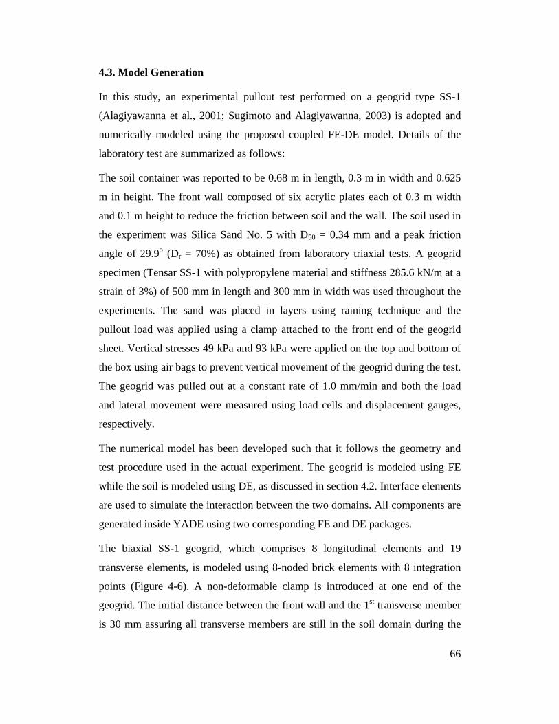
4.3. Model Generation
In this study, an experimental pullout test performed on a geogrid type SS-1
(Alagiyawanna et al., 2001; Sugimoto and Alagiyawanna, 2003) is adopted and
numerically modeled using the proposed coupled FE-DE model. Details of the
laboratory test are summarized as follows:
The soil container was reported to be 0.68 m in length, 0.3 m in width and 0.625
m in height. The front wall composed of six acrylic plates each of 0.3 m width
and 0.1 m height to reduce the friction between soil and the wall. The soil used in
the experiment was Silica Sand No. 5 with D50 = 0.34 mm and a peak friction
angle of 29.9o (Dr = 70%) as obtained from laboratory triaxial tests. A geogrid
specimen (Tensar SS-1 with polypropylene material and stiffness 285.6 kN/m at a
strain of 3%) of 500 mm in length and 300 mm in width was used throughout the
experiments. The sand was placed in layers using raining technique and the
pullout load was applied using a clamp attached to the front end of the geogrid
sheet. Vertical stresses 49 kPa and 93 kPa were applied on the top and bottom of
the box using air bags to prevent vertical movement of the geogrid during the test.
The geogrid was pulled out at a constant rate of 1.0 mm/min and both the load
and lateral movement were measured using load cells and displacement gauges,
respectively.
The numerical model has been developed such that it follows the geometry and
test procedure used in the actual experiment. The geogrid is modeled using FE
while the soil is modeled using DE, as discussed in section 4.2. Interface elements
are used to simulate the interaction between the two domains. All components are
generated inside YADE using two corresponding FE and DE packages.
The biaxial SS-1 geogrid, which comprises 8 longitudinal elements and 19
transverse elements, is modeled using 8-noded brick elements with 8 integration
points (Figure 4-6). A non-deformable clamp is introduced at one end of the
geogrid. The initial distance between the front wall and the 1st transverse member
is 30 mm assuring all transverse members are still in the soil domain during the
66
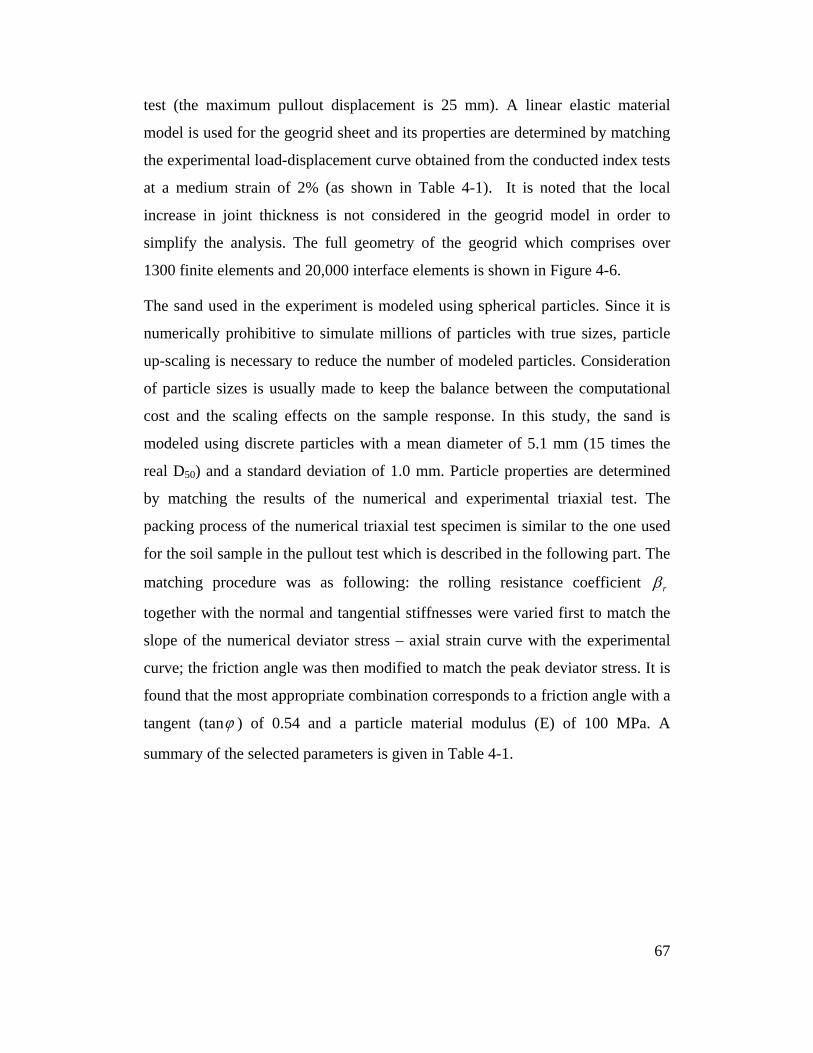
test (the maximum pullout displacement is 25 mm). A linear elastic material
model is used for the geogrid sheet and its properties are determined by matching
the experimental load-displacement curve obtained from the conducted index tests
at a medium strain of 2% (as shown in Table 4-1). It is noted that the local
increase in joint thickness is not considered in the geogrid model in order to
simplify the analysis. The full geometry of the geogrid which comprises over
1300 finite elements and 20,000 interface elements is shown in Figure 4-6.
The sand used in the experiment is modeled using spherical particles. Since it is
numerically prohibitive to simulate millions of particles with true sizes, particle
up-scaling is necessary to reduce the number of modeled particles. Consideration
of particle sizes is usually made to keep the balance between the computational
cost and the scaling effects on the sample response. In this study, the sand is
modeled using discrete particles with a mean diameter of 5.1 mm (15 times the
real D50) and a standard deviation of 1.0 mm. Particle properties are determined
by matching the results of the numerical and experimental triaxial test. The
packing process of the numerical triaxial test specimen is similar to the one used
for the soil sample in the pullout test which is described in the following part. The
matching procedure was as following: the rolling resistance coefficient rβ
together with the normal and tangential stiffnesses were varied first to match the
slope of the numerical deviator stress – axial strain curve with the experimental
curve; the friction angle was then modified to match the peak deviator stress. It is
found that the most appropriate combination corresponds to a friction angle with a
tangent (tanϕ ) of 0.54 and a particle material modulus (E) of 100 MPa. A
summary of the selected parameters is given in Table 4-1.
67
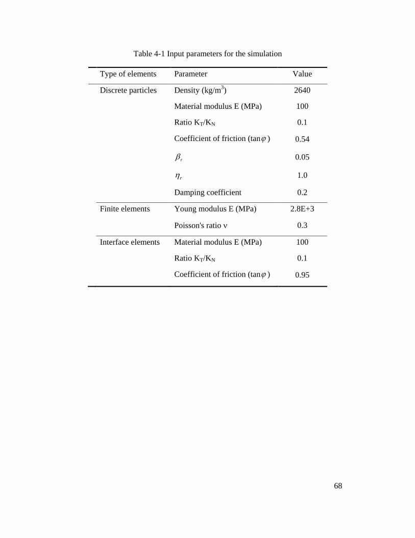
Table 4-1 Input parameters for the simulation
Type of elements Parameter Value
Discrete particles Density (kg/m3) 2640
Material modulus E (MPa) 100
Ratio KT/KN 0.1
Coefficient of friction (tanϕ ) 0.54
rβ 0.05
rη 1.0
Damping coefficient 0.2
Finite elements Young modulus E (MPa) 2.8E+3
Poisson's ratio ν 0.3
Interface elements Material modulus E (MPa) 100
Ratio KT/KN 0.1
Coefficient of friction (tanϕ ) 0.95
68
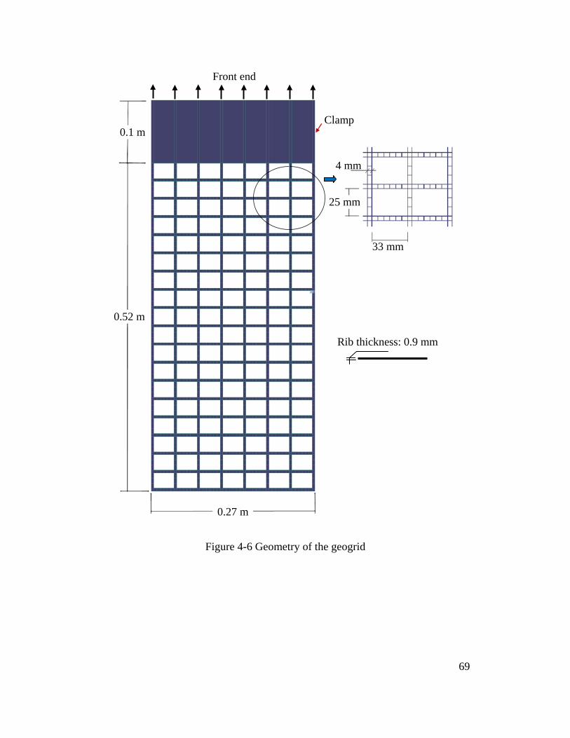
Figure 4-6 Geometry of the geogrid
0.27 m
0.52 m
33 mm
25 mm
4 mm
Rib thickness: 0.9 mm
Front end
Clamp 0.1 m
69
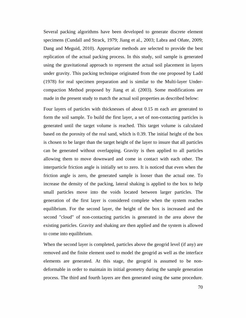
Several packing algorithms have been developed to generate discrete element
specimens (Cundall and Strack, 1979; Jiang et al., 2003; Labra and Oñate, 2009;
Dang and Meguid, 2010). Appropriate methods are selected to provide the best
replication of the actual packing process. In this study, soil sample is generated
using the gravitational approach to represent the actual soil placement in layers
under gravity. This packing technique originated from the one proposed by Ladd
(1978) for real specimen preparation and is similar to the Multi-layer Under-
compaction Method proposed by Jiang et al. (2003). Some modifications are
made in the present study to match the actual soil properties as described below:
Four layers of particles with thicknesses of about 0.15 m each are generated to
form the soil sample. To build the first layer, a set of non-contacting particles is
generated until the target volume is reached. This target volume is calculated
based on the porosity of the real sand, which is 0.39. The initial height of the box
is chosen to be larger than the target height of the layer to insure that all particles
can be generated without overlapping. Gravity is then applied to all particles
allowing them to move downward and come in contact with each other. The
interparticle friction angle is initially set to zero. It is noticed that even when the
friction angle is zero, the generated sample is looser than the actual one. To
increase the density of the packing, lateral shaking is applied to the box to help
small particles move into the voids located between larger particles. The
generation of the first layer is considered complete when the system reaches
equilibrium. For the second layer, the height of the box is increased and the
second "cloud" of non-contacting particles is generated in the area above the
existing particles. Gravity and shaking are then applied and the system is allowed
to come into equilibrium.
When the second layer is completed, particles above the geogrid level (if any) are
removed and the finite element used to model the geogrid as well as the interface
elements are generated. At this stage, the geogrid is assumed to be non-
deformable in order to maintain its initial geometry during the sample generation
process. The third and fourth layers are then generated using the same procedure.
70
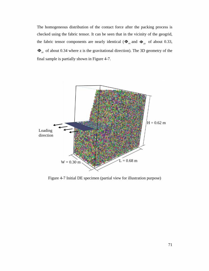
The homogeneous distribution of the contact force after the packing process is
checked using the fabric tensor. It can be seen that in the vicinity of the geogrid,
the fabric tensor components are nearly identical ( xxΦ and yyΦ of about 0.33,
zzΦ of about 0.34 where z is the gravitational direction). The 3D geometry of the
final sample is partially shown in Figure 4-7.
Figure 4-7 Initial DE specimen (partial view for illustration purpose)
L = 0.68 m
H = 0.62 m
W = 0.30 m
Loading direction
71
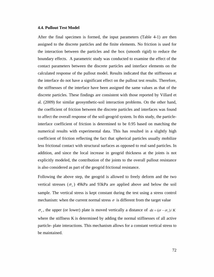
4.4. Pullout Test Model
After the final specimen is formed, the input parameters (Table 4-1) are then
assigned to the discrete particles and the finite elements. No friction is used for
the interaction between the particles and the box (smooth rigid) to reduce the
boundary effects. A parametric study was conducted to examine the effect of the
contact parameters between the discrete particles and interface elements on the
calculated response of the pullout model. Results indicated that the stiffnesses at
the interface do not have a significant effect on the pullout test results. Therefore,
the stiffnesses of the interface have been assigned the same values as that of the
discrete particles. These findings are consistent with those reported by Villard et
al. (2009) for similar geosynthetic-soil interaction problems. On the other hand,
the coefficient of friction between the discrete particles and interfaces was found
to affect the overall response of the soil-geogrid system. In this study, the particle-
interface coefficient of friction is determined to be 0.95 based on matching the
numerical results with experimental data. This has resulted in a slightly high
coefficient of friction reflecting the fact that spherical particles usually mobilize
less frictional contact with structural surfaces as opposed to real sand particles. In
addition, and since the local increase in geogrid thickness at the joints is not
explicitly modeled, the contribution of the joints to the overall pullout resistance
is also considered as part of the geogrid frictional resistance.
Following the above step, the geogrid is allowed to freely deform and the two
vertical stresses ( vσ ) 49kPa and 93kPa are applied above and below the soil
sample. The vertical stress is kept constant during the test using a stress control
mechanism: when the current normal stress σ is different from the target value
vσ , the upper (or lower) plate is moved vertically a distance of ( ) /vdz Kσ σ= −
where the stiffness K is determined by adding the normal stiffnesses of all active
particle- plate interactions. This mechanism allows for a constant vertical stress to
be maintained.
72
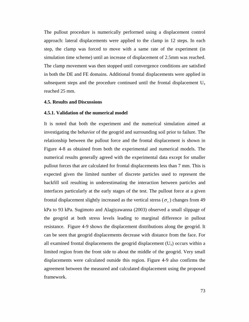
The pullout procedure is numerically performed using a displacement control
approach: lateral displacements were applied to the clamp in 12 steps. In each
step, the clamp was forced to move with a same rate of the experiment (in
simulation time scheme) until an increase of displacement of 2.5mm was reached.
The clamp movement was then stopped until convergence conditions are satisfied
in both the DE and FE domains. Additional frontal displacements were applied in
subsequent steps and the procedure continued until the frontal displacement Ux
reached 25 mm.
4.5. Results and Discussions
4.5.1. Validation of the numerical model
It is noted that both the experiment and the numerical simulation aimed at
investigating the behavior of the geogrid and surrounding soil prior to failure. The
relationship between the pullout force and the frontal displacement is shown in
Figure 4-8 as obtained from both the experimental and numerical models. The
numerical results generally agreed with the experimental data except for smaller
pullout forces that are calculated for frontal displacements less than 7 mm. This is
expected given the limited number of discrete particles used to represent the
backfill soil resulting in underestimating the interaction between particles and
interfaces particularly at the early stages of the test. The pullout force at a given
frontal displacement slightly increased as the vertical stress ( vσ ) changes from 49
kPa to 93 kPa. Sugimoto and Alagiyawanna (2003) observed a small slippage of
the geogrid at both stress levels leading to marginal difference in pullout
resistance. Figure 4-9 shows the displacement distributions along the geogrid. It
can be seen that geogrid displacements decrease with distance from the face. For
all examined frontal displacements the geogrid displacement (Ux) occurs within a
limited region from the front side to about the middle of the geogrid. Very small
displacements were calculated outside this region. Figure 4-9 also confirms the
agreement between the measured and calculated displacement using the proposed
framework.
73
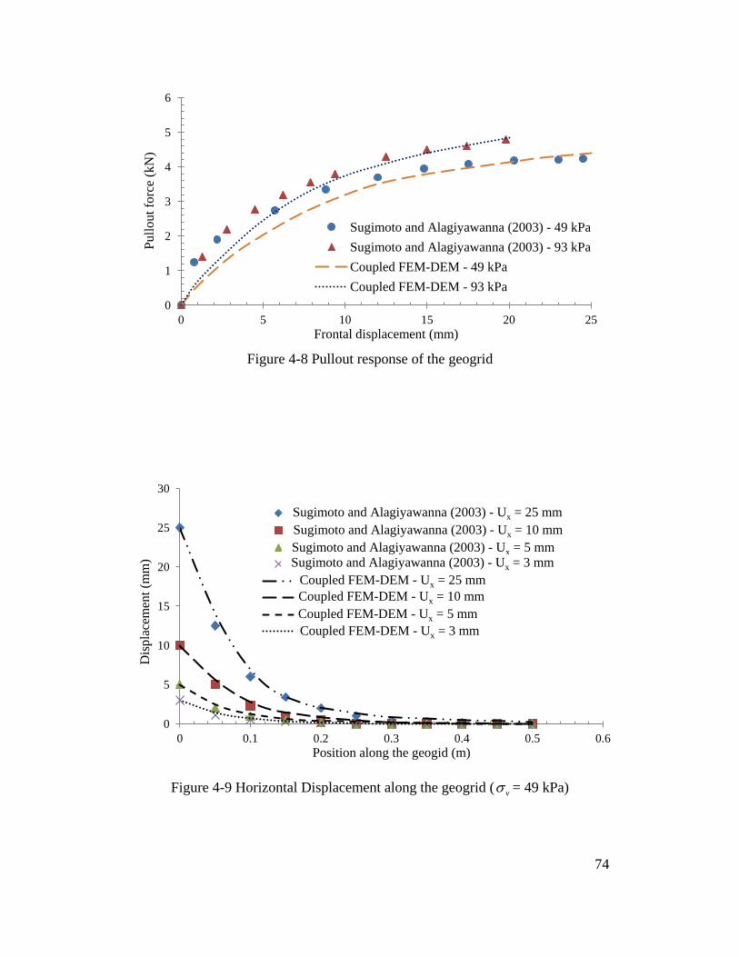
Figure 4-8 Pullout response of the geogrid
Figure 4-9 Horizontal Displacement along the geogrid ( vσ = 49 kPa)
0
1
2
3
4
5
6
0 5 10 15 20 25
Pullo
ut fo
rce
(kN
)
Frontal displacement (mm)
Sugimoto and Alagiyawanna (2003) - 49 kPa Sugimoto and Alagiyawanna (2003) - 93 kPa Coupled FEM-DEM - 49 kPa Coupled FEM-DEM - 93 kPa
0
5
10
15
20
25
30
0 0.1 0.2 0.3 0.4 0.5 0.6
Dis
plac
emen
t (m
m)
Position along the geogid (m)
Experiment - Ux = 25 mm Experiment - Ux = 10 mm Experiment - Ux = 5 mm Experiment - Ux = 3 mm Coupled DEM/FEM - Ux = 25 mm Coupled DEM/FEM - Ux = 10 mm Coupled DEM/FEM - Ux = 5 mm Coupled DEM/FEM - Ux = 3 mm
Sugimoto and Alagiyawanna (2003) - Ux = 25 mm Sugimoto and Alagiyawanna (2003) - Ux = 10 mm Sugimoto and Alagiyawanna (2003) - Ux = 5 mm Sugimoto and Alagiyawanna (2003) - Ux = 3 mm
Coupled FEM-DEM - Ux = 25 mm Coupled FEM-DEM - Ux = 10 mm Coupled FEM-DEM - Ux = 5 mm Coupled FEM-DEM - Ux = 3 mm
74
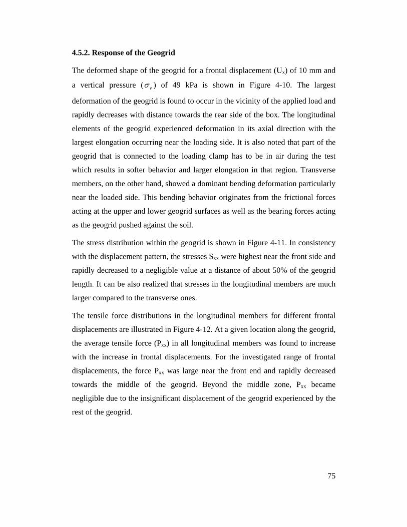
4.5.2. Response of the Geogrid
The deformed shape of the geogrid for a frontal displacement (Ux) of 10 mm and
a vertical pressure ( vσ ) of 49 kPa is shown in Figure 4-10. The largest
deformation of the geogrid is found to occur in the vicinity of the applied load and
rapidly decreases with distance towards the rear side of the box. The longitudinal
elements of the geogrid experienced deformation in its axial direction with the
largest elongation occurring near the loading side. It is also noted that part of the
geogrid that is connected to the loading clamp has to be in air during the test
which results in softer behavior and larger elongation in that region. Transverse
members, on the other hand, showed a dominant bending deformation particularly
near the loaded side. This bending behavior originates from the frictional forces
acting at the upper and lower geogrid surfaces as well as the bearing forces acting
as the geogrid pushed against the soil.
The stress distribution within the geogrid is shown in Figure 4-11. In consistency
with the displacement pattern, the stresses Sxx were highest near the front side and
rapidly decreased to a negligible value at a distance of about 50% of the geogrid
length. It can be also realized that stresses in the longitudinal members are much
larger compared to the transverse ones.
The tensile force distributions in the longitudinal members for different frontal
displacements are illustrated in Figure 4-12. At a given location along the geogrid,
the average tensile force (Pxx) in all longitudinal members was found to increase
with the increase in frontal displacements. For the investigated range of frontal
displacements, the force Pxx was large near the front end and rapidly decreased
towards the middle of the geogrid. Beyond the middle zone, Pxx became
negligible due to the insignificant displacement of the geogrid experienced by the
rest of the geogrid.
75
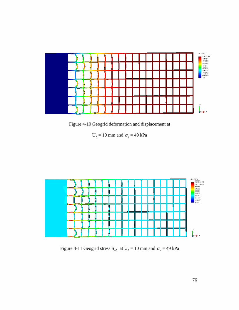
Figure 4-10 Geogrid deformation and displacement at
Ux = 10 mm and vσ = 49 kPa
Figure 4-11 Geogrid stress Sxx at Ux = 10 mm and vσ = 49 kPa
76
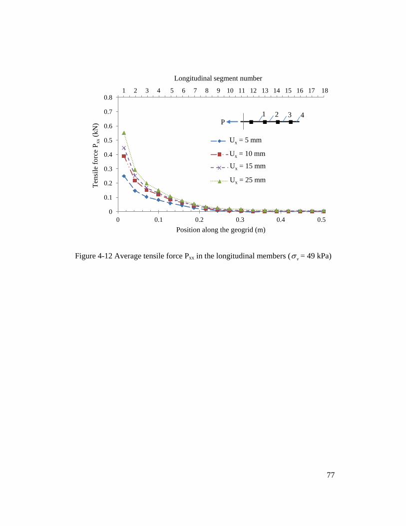
Figure 4-12 Average tensile force Pxx in the longitudinal members ( vσ = 49 kPa)
0
0.1
0.2
0.3
0.4
0.5
0.6
0.7
0.8
0 0.1 0.2 0.3 0.4 0.5
Longitudinal segment number
Tens
ile fo
rce
P xx (
kN)
Position along the geogrid (m)
Ux = 5 mm
Ux = 10 mm
Ux = 15 mm
Ux = 25 mm
1 2 3 4 5 6 7 8 9 10 11 12 13 14 15 16 17 18
Ux = 5 mm
Ux = 10 mm
Ux = 15 mm
Ux = 25 mm
1 2 3 4 P
77
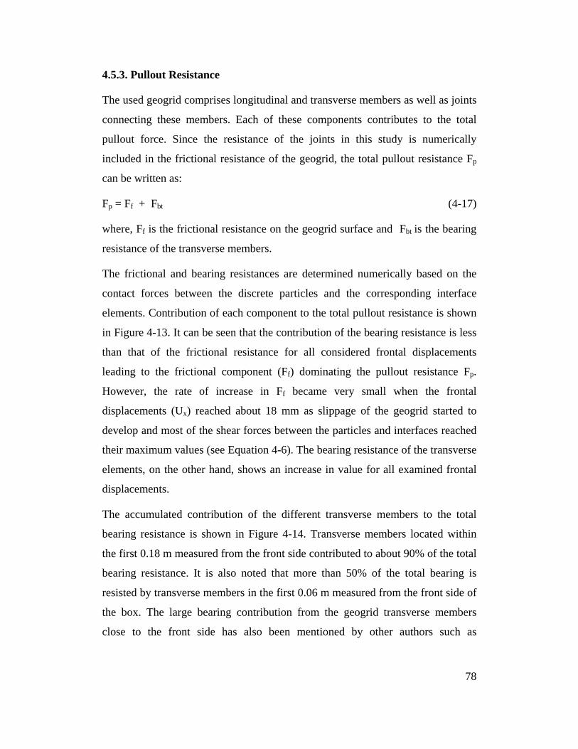
4.5.3. Pullout Resistance
The used geogrid comprises longitudinal and transverse members as well as joints
connecting these members. Each of these components contributes to the total
pullout force. Since the resistance of the joints in this study is numerically
included in the frictional resistance of the geogrid, the total pullout resistance Fp
can be written as:
Fp = Ff + Fbt (4-17)
where, Ff is the frictional resistance on the geogrid surface and Fbt is the bearing
resistance of the transverse members.
The frictional and bearing resistances are determined numerically based on the
contact forces between the discrete particles and the corresponding interface
elements. Contribution of each component to the total pullout resistance is shown
in Figure 4-13. It can be seen that the contribution of the bearing resistance is less
than that of the frictional resistance for all considered frontal displacements
leading to the frictional component (Ff) dominating the pullout resistance Fp.
However, the rate of increase in Ff became very small when the frontal
displacements (Ux) reached about 18 mm as slippage of the geogrid started to
develop and most of the shear forces between the particles and interfaces reached
their maximum values (see Equation 4-6). The bearing resistance of the transverse
elements, on the other hand, shows an increase in value for all examined frontal
displacements.
The accumulated contribution of the different transverse members to the total
bearing resistance is shown in Figure 4-14. Transverse members located within
the first 0.18 m measured from the front side contributed to about 90% of the total
bearing resistance. It is also noted that more than 50% of the total bearing is
resisted by transverse members in the first 0.06 m measured from the front side of
the box. The large bearing contribution from the geogrid transverse members
close to the front side has also been mentioned by other authors such as
78

Costalonga (1988 and 1990), Milligan et al. (1990) and Palmeira (1987, 2004 and
2009).
79
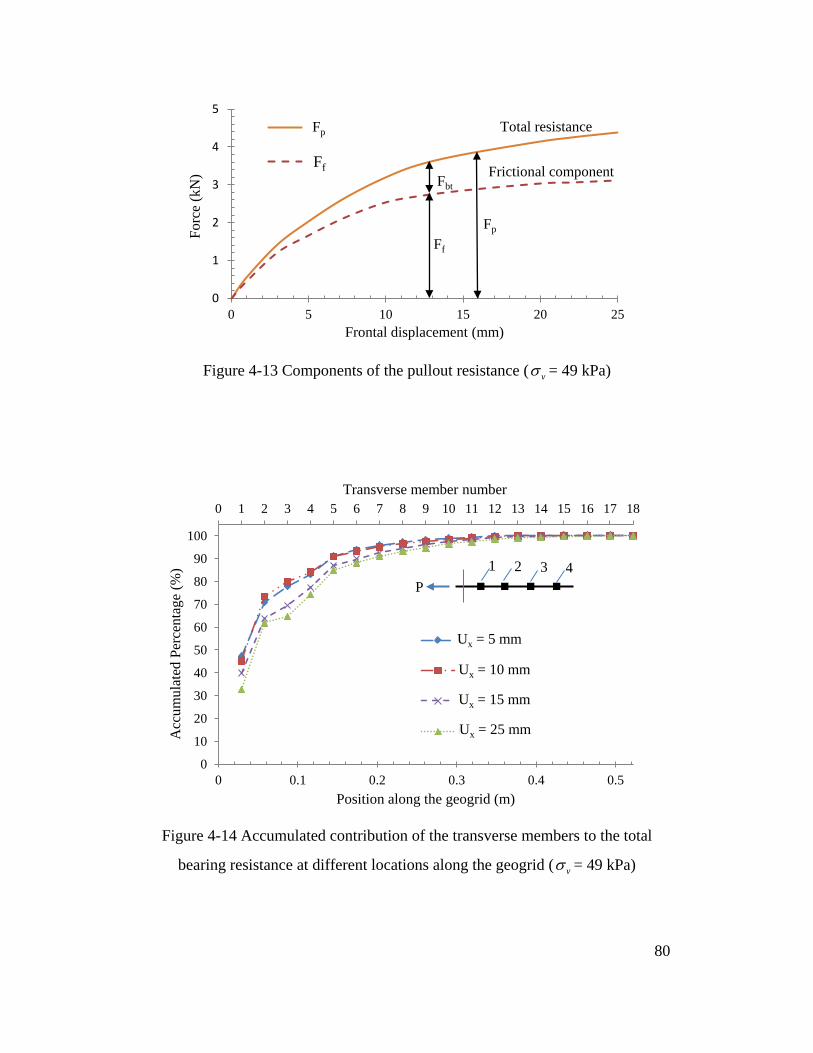
Figure 4-13 Components of the pullout resistance ( vσ = 49 kPa)
Figure 4-14 Accumulated contribution of the transverse members to the total
bearing resistance at different locations along the geogrid ( vσ = 49 kPa)
0
1
2
3
4
5
0 5 10 15 20 25
Forc
e (k
N)
Frontal displacement (mm)
Fp
Ff Fbt
Ff
Fp
Fp
Ff
Total resistance
Frictional component
0 1 2 3 4 5 6 7 8 9 10 11 12 13 14 15 16 17 18
0
10
20
30
40
50
60
70
80
90
100
0 0.1 0.2 0.3 0.4 0.5
Transverse member number
Acc
umul
ated
Per
cent
age
(%)
Position along the geogrid (m)
Ux = 5 mm
Ux = 10 mm
Ux = 15 mm
Ux = 25 mm
Ux = 5 mm
Ux = 10 mm
Ux = 15 mm
Ux = 25 mm
P 1 2 3 4
80
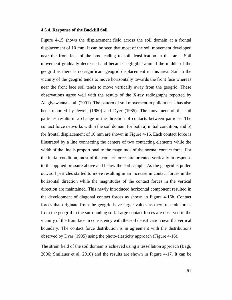
4.5.4. Response of the Backfill Soil
Figure 4-15 shows the displacement field across the soil domain at a frontal
displacement of 10 mm. It can be seen that most of the soil movement developed
near the front face of the box leading to soil densification in that area. Soil
movement gradually decreased and became negligible around the middle of the
geogrid as there is no significant geogrid displacement in this area. Soil in the
vicinity of the geogrid tends to move horizontally towards the front face whereas
near the front face soil tends to move vertically away from the geogrid. These
observations agree well with the results of the X-ray radiographs reported by
Alagiyawanna et al. (2001). The pattern of soil movement in pullout tests has also
been reported by Jewell (1980) and Dyer (1985). The movement of the soil
particles results in a change in the direction of contacts between particles. The
contact force networks within the soil domain for both a) initial condition; and b)
for frontal displacement of 10 mm are shown in Figure 4-16. Each contact force is
illustrated by a line connecting the centers of two contacting elements while the
width of the line is proportional to the magnitude of the normal contact force. For
the initial condition, most of the contact forces are oriented vertically in response
to the applied pressure above and below the soil sample. As the geogrid is pulled
out, soil particles started to move resulting in an increase in contact forces in the
horizontal direction while the magnitudes of the contact forces in the vertical
direction are maintained. This newly introduced horizontal component resulted in
the development of diagonal contact forces as shown in Figure 4-16b. Contact
forces that originate from the geogrid have larger values as they transmit forces
from the geogrid to the surrounding soil. Large contact forces are observed in the
vicinity of the front face in consistency with the soil densification near the vertical
boundary. The contact force distribution is in agreement with the distributions
observed by Dyer (1985) using the photo-elasticity approach (Figure 4-16).
The strain field of the soil domain is achieved using a tessellation approach (Bagi,
2006; Šmilauer et al. 2010) and the results are shown in Figure 4-17. It can be
81
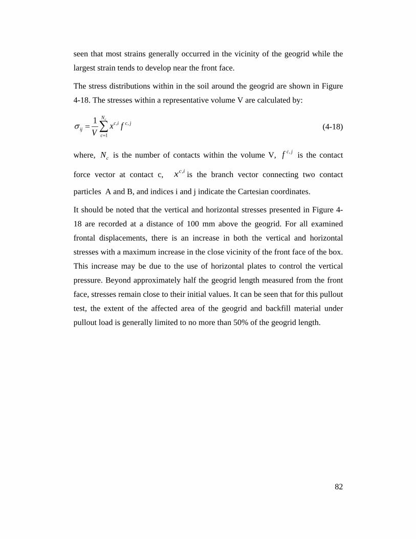
seen that most strains generally occurred in the vicinity of the geogrid while the
largest strain tends to develop near the front face.
The stress distributions within in the soil around the geogrid are shown in Figure
4-18. The stresses within a representative volume V are calculated by:
, ,
1
1 cNc i c j
ijc
x fV
σ=
= ∑ (4-18)
where, cN is the number of contacts within the volume V, jcf , is the contact
force vector at contact c, icx , is the branch vector connecting two contact
particles A and B, and indices i and j indicate the Cartesian coordinates.
It should be noted that the vertical and horizontal stresses presented in Figure 4-
18 are recorded at a distance of 100 mm above the geogrid. For all examined
frontal displacements, there is an increase in both the vertical and horizontal
stresses with a maximum increase in the close vicinity of the front face of the box.
This increase may be due to the use of horizontal plates to control the vertical
pressure. Beyond approximately half the geogrid length measured from the front
face, stresses remain close to their initial values. It can be seen that for this pullout
test, the extent of the affected area of the geogrid and backfill material under
pullout load is generally limited to no more than 50% of the geogrid length.
82
Figure 4-15 Displacement field of the soil domain at Ux = 10 mm and vσ = 49 kPa
0.0 0.1 0.2 0.3 0.4 0.5 0.6
Distance from front face (m)
0.2
0.1
0.0
-0.1
-0.2
Dis
tanc
e fr
om b
ase
(m)
83
Figure 4-16 Contact force networks within the soil around the geogrid
a) Contact-force network at the initial condition ( 49v kPaσ = )
b) Contact-force network at Ux = 10 mm ( 49v kPaσ = )
84
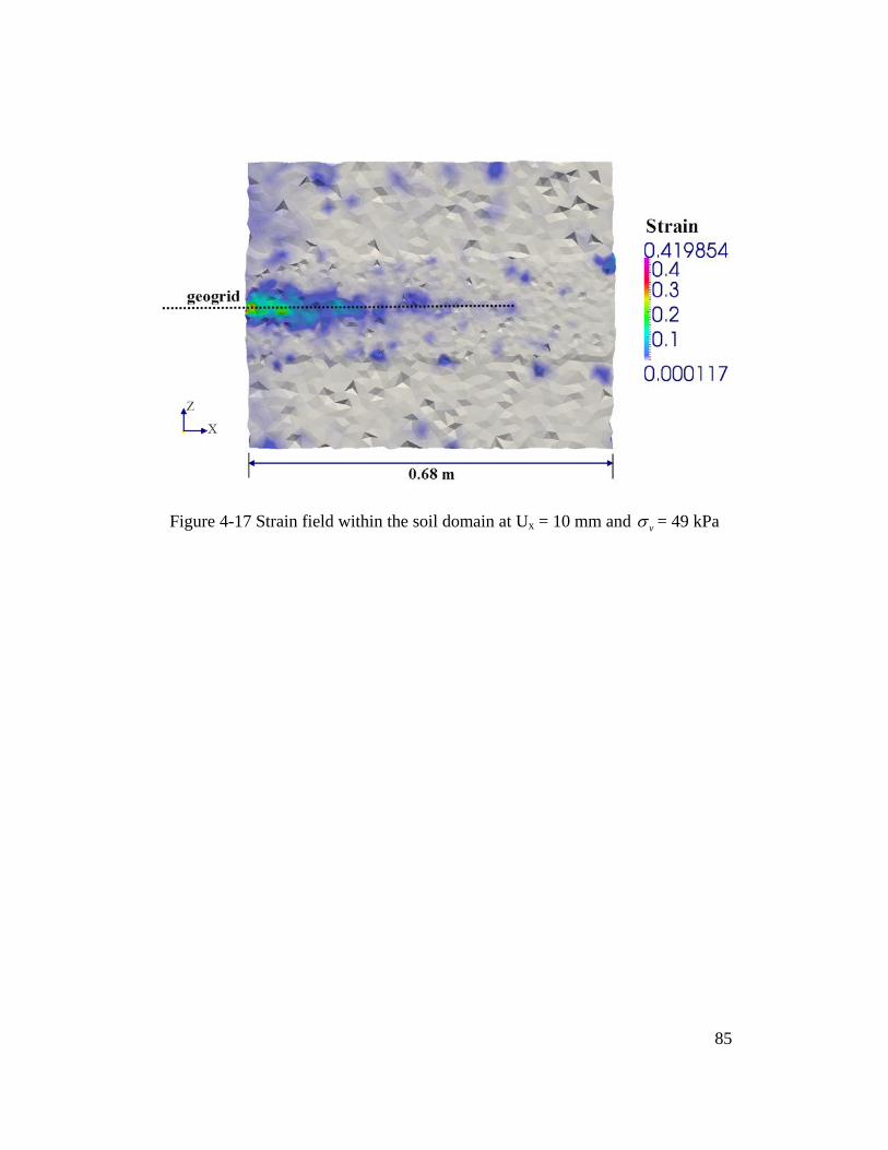
Figure 4-17 Strain field within the soil domain at Ux = 10 mm and vσ = 49 kPa
85
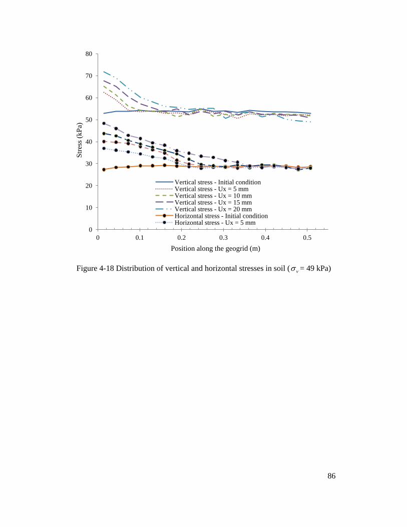
Figure 4-18 Distribution of vertical and horizontal stresses in soil ( vσ = 49 kPa)
0
10
20
30
40
50
60
70
80
0 0.1 0.2 0.3 0.4 0.5
Stre
ss (k
Pa)
Position along the geogrid (m)
Vertical stress - Initial condition Vertical stress - Ux = 5 mm Vertical stress - Ux = 10 mm Vertical stress - Ux = 15 mm Vertical stress - Ux = 20 mm Horizontal stress - Initial condition Horizontal stress - Ux = 5 mm
86
4.6. Summary and Conclusions
In this paper, a framework for coupling finite and discrete element methods was
developed. Interface elements were introduced to ensure the transmission of
forces between the DE and FE domains. A multiple-time-step scheme was applied
to optimize the computational cost. Using the developed framework, a three-
dimensional numerical study was performed to investigate the behavior of a
biaxial geogrid embedded in granular material under pullout loading condition.
The geogrid was modeled using finite elements while the backfill material was
modeled using discrete elements. The results of the analysis were compared with
experimental data. The displacements and stresses developing in the geogrid were
analyzed and the micro-mechanical behavior of the soil domain was investigated.
Most of the geogrid stresses and displacements occurred near the front side of the
box with rapid decrease with distance and reached very small values around the
middle of the geogrid. For the investigated geogrid and soil conditions, the
contribution of the frictional resistance to the total pullout resistance was found to
be larger than the bearing resistance. The contribution of the bearing resistance to
the overall capacity increased as the geogrid displacement increased. The soil
movement and the contact force distribution within the soil domain agreed with
experimental observations. An increase in soil stresses and strains was observed
near the front face.
Finally, the proposed coupled FE-DE method has proven to be efficient to model
the pullout experiment in three-dimensional space and capture the response of
both the geogrid and the surrounding backfill material.
87
Preface to Chapter 5
The developed coupled Finite-Discrete element framework has demonstrated its
efficiency in investigating the 3D response of soil-geogrid interaction under
geogrid pullout testing condition. To continually demonstrate the robustness of
the coupled Finite-Discrete element algorithm, the framework is now used to
analyze a strip footing over geogrid-reinforced sand. Both unreinforced and
geogrid reinforced foundations are studied from which the efficiency of geogrid
reinforcement is investigated. The capability of the framework to model the soil-
geogrid interaction at the microscopic scale is demonstrated.
88
CHAPTER 5
Three-Dimensional Analysis of Geogrid Reinforced Foundation Using Finite-Discrete Element Framework *
Abstract
Three-dimensional analysis of soil-structure interaction problems considering the
detailed response at the particle scale level is a challenging numerical modeling
problem. An efficient numerical framework that takes advantage of both the finite
and discrete element approaches to investigate soil-geogrid interaction is
described in this paper. The method uses finite elements to model the structural
components and discrete particles to model the surrounding soil to reflect the
discontinuous nature of the granular material. The coupled framework is used to
investigate the behavior of strip footing over geogrid-reinforced sand. The
numerical results are validated using experimental data. New insight into the
three-dimensional interaction between the soil and the geogrid is presented.
Keywords: geogrid reinforcement, finite-discrete element, strip foundation,
numerical simulation.
* A version of this chapter has been submitted to International Journal of
Geomechanics ASCE, 2013.
89
5.1. Introduction
Continuum approaches (e.g., Finite Element and Finite Difference) are generally
used for the numerical analysis of soil-structure interaction problems. The finite
element method (FE) has proven to be a powerful tool to model both structural
elements and the surrounding soil. Although FE can be used efficiently to model
the soil behavior at the macroscopic scale, the discontinuous nature of the soil
particles is not easy to represent. This discontinuous nature has an important role
in the behavior of different soil-structure interaction systems such as soil-geogrid
interlocking (McDowell et al., 2006), soil arching in embankments (Han et al.,
2011) and particle erosion in the vicinity of subsurface structures (Meguid and
Dang, 2009). The discrete element method (DE) proposed by Cundall and Strack
(1979) is an alternative approach for the modeling of these systems. While the DE
method can efficiently model soil discontinuous behavior (Maynar and
Rodríguez, 2005; Lobo-Guerrero and Vallejo; 2006; Tran et al., 2012), using the
DE method to model structural elements can lead to inaccurate responses.
Researches including McDowell et al. (2006), Han et al. (2011) and Chen et al.
(2012), used sets of discrete particles bonded together to model structural
components. However, since micro voids generally develop in a structure
generated by bonded particles, the continuous nature of the structure may not be
fully captured.
To take advantage of both FE and DE methods, the structure can be modeled
using FE whereas the soil can be modeled using the DE method. The coupling of
the two methods can efficiently model the behavior of both the soil and the
structure. This approach has been used by several researchers to analyze certain
geotechnical problems. Elmekati and Shamy (2010) used this approach to model
pile installation in which the pile was modeled using FE while the surrounding
soil was modeled using DE. Dang and Meguid (2013) studied the earth pressure
distribution on tunnel linings by modeling the tunnel lining using FE and
surrounding soil using DE. Geotextile-reinforced embankment analysis using a
coupled framework was reported by Villard et al. (2009). Soil-geogrid interaction
90
during the geogrid pullout process was studied by Tran et al. (2013). The geogrid
was modeled using FE representing the 3D geometry of the geogrid whereas the
backfill soil was modeled using DE. The soil-geogrid interaction was ensured
using interface elements. In this paper, a coupled Finite-Discrete element (FE-DE)
framework that is capable of modeling soil-structure interaction problems at the
microscopic scale level is used to investigate the behavior of foundation over
reinforced soil. Literature review of the investigated problem is presented below.
Over the past three decades, the use of geosynthetics to increase bearing capacity
of shallow foundations has received extensive research attention. The bearing
capacity of reinforced soil has been studied experimentally by many researches
across the world, including Guido et al. (1986), Huang and Tatsuoka (1990),
Khing et al. (1993), Shin et al. (1993), Das et al.(1994), Yetimoglu et al. (1994),
Adams and Collin (1997), Dash et al. (2001), DeMerchant et al. (2002), Patra et
al. (2006), Basudhar et al. (2007), Chen et al. (2007), Chen et al. (2009), Abu-
Farsakh et al. (2008), Ghazavi and Lavasan (2008), Ghosh and Dey (2009), Latha
and Somwanshi (2009a, b), Sadoglu et al. (2009), Choudhary et al. (2010),
Mohamed (2010) and Tafreshi and Dawson (2010). Results from these
experimental studies show that the bearing capacity of a given foundation
generally increases with the placement of geosynthetic material within the
supporting ground. The effects of different variables such as geosynthetic length,
vertical spacing between multiple reinforcing layers, depth to the top layer,
number of layers and types of geosynthetics that contribute to the bearing
capacity were also examined. Analytical solutions were also developed by
Binquet and Lee (1975a,b), Michalowski (2004), Wayne et al. (1998), Kumar and
Saran (2003), Abu-Farsakh et al. (2008), Huang and Menq (1997) and Sharma et
al. (2009). Numerical simulation is an alternative way to study the stresses and
strains within soil and in the geosynthetic layers. Finite element modeling of
reinforced foundations has been reported by Yetimoglu et al. (1994), Kurian et al.
(1997), Siddiquee and Huang (2001), Yamamoto and Otani (2002), Basudhar et
al. (2007), Chung and Cascante (2007), Ghazavi and Lavasan (2008), Latha and
91
Somwanshi (2009a, b) and Li et al. (2012). In these studies, the reinforcement
was often simplified either as a truss structure (in 2D analysis) or a continuous
sheet (in 3D analysis). This simplification does not represent the true geometry of
the geosynthetics particularly for geogrids. The interaction between geogrid and
the surrounding soil was often modeled using interface elements in which contact
properties were considered while the interlocking effect is not generally
represented. It is known that the soil-geogrid interlocking in reinforced soils plays
an important role in the bearing capacity of the foundation (Guido et al., 1986).
The interlocking of the soil particles through the apertures of the grid mobilizes
tensile strength in the reinforcing layer and generate anchoring effect in the soil-
geogrid system. This leads to better geotechnical performance compared to
geotextile-reinforced soil foundations. The coupled FE-DE approach presented in
this study allows for the interlocking effect to be explicitly simulated considering
the soils as DE particles while the 3D geometry of the geogrid is represented
using FE elements. The interaction between the two domains is ensured using
interface elements.
5.2. Model Generation
In this study, the experimental results reported by Das et al. (1994) and Khing et
al. (1993) of a strip foundation supported by geogrid-reinforced sand is used to
validate the proposed coupled FE-DE model. The soil container was reported to
be 1.1m in length, 0.3m in width and 0.9m in height. The walls were polished to
reduce the friction between the soil and the wall. The strip foundation had a width
of 76 mm (noted as B) and a length of 300 mm. A rough condition at the base of
the foundation was generated by cementing a thin layer of sand at the contact
surface. The soil used in the experiment was medium-grained silica sand with D50
= 0.51 mm, average dry unit weight of 17.14 kN/m3 and a peak friction angle of
41o (at Dr = 70%) obtained from laboratory direct shear tests. Biaxial geogrids
(Tensar SS-0 with PP/HDPE copolymer material and tensile modulus of 182
kN/m at 2% strain) of 760 mm in length and 300mm in width were used in the
experiment. The top geogrid layer was installed at a depth 25 mm (0.33B) below
92
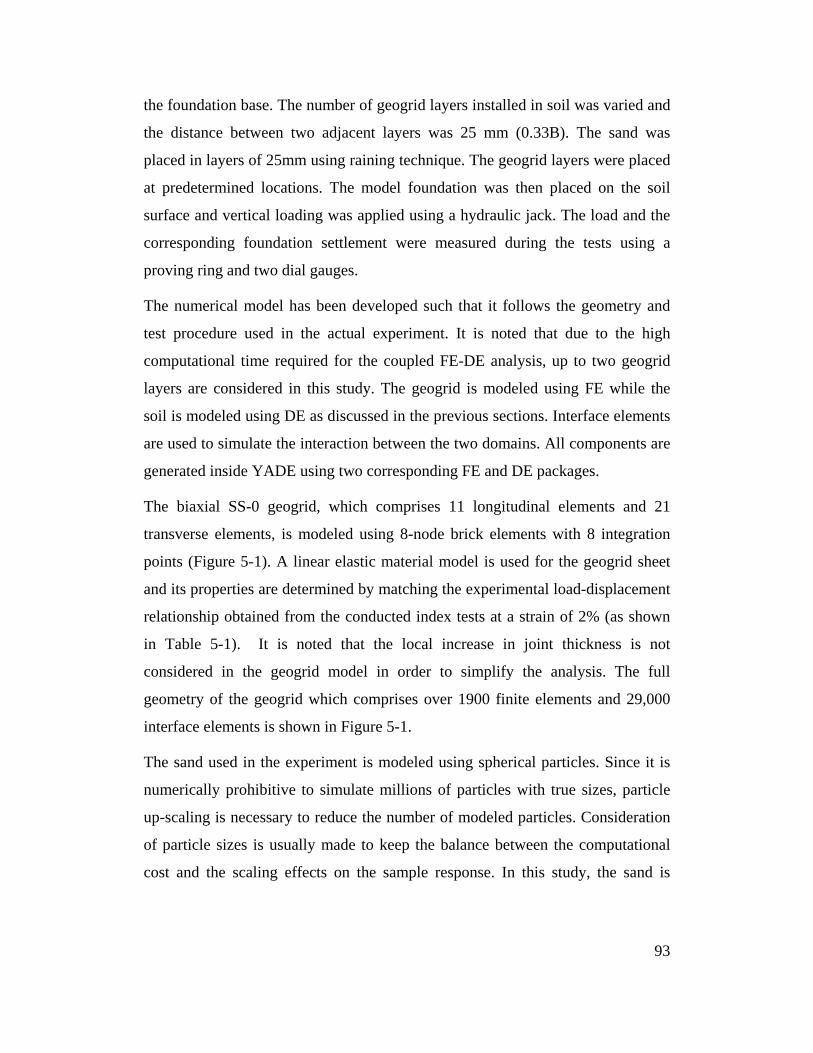
the foundation base. The number of geogrid layers installed in soil was varied and
the distance between two adjacent layers was 25 mm (0.33B). The sand was
placed in layers of 25mm using raining technique. The geogrid layers were placed
at predetermined locations. The model foundation was then placed on the soil
surface and vertical loading was applied using a hydraulic jack. The load and the
corresponding foundation settlement were measured during the tests using a
proving ring and two dial gauges.
The numerical model has been developed such that it follows the geometry and
test procedure used in the actual experiment. It is noted that due to the high
computational time required for the coupled FE-DE analysis, up to two geogrid
layers are considered in this study. The geogrid is modeled using FE while the
soil is modeled using DE as discussed in the previous sections. Interface elements
are used to simulate the interaction between the two domains. All components are
generated inside YADE using two corresponding FE and DE packages.
The biaxial SS-0 geogrid, which comprises 11 longitudinal elements and 21
transverse elements, is modeled using 8-node brick elements with 8 integration
points (Figure 5-1). A linear elastic material model is used for the geogrid sheet
and its properties are determined by matching the experimental load-displacement
relationship obtained from the conducted index tests at a strain of 2% (as shown
in Table 5-1). It is noted that the local increase in joint thickness is not
considered in the geogrid model in order to simplify the analysis. The full
geometry of the geogrid which comprises over 1900 finite elements and 29,000
interface elements is shown in Figure 5-1.
The sand used in the experiment is modeled using spherical particles. Since it is
numerically prohibitive to simulate millions of particles with true sizes, particle
up-scaling is necessary to reduce the number of modeled particles. Consideration
of particle sizes is usually made to keep the balance between the computational
cost and the scaling effects on the sample response. In this study, the sand is
93
modeled using discrete particles with a mean diameter of 10.2 mm (20 times the
real D50) and a standard deviation of 2.0 mm.
To generate DE samples, appropriate packing methods are considered to provide
the best replication of the actual packing process. Several packing algorithms
have been developed to generate discrete element specimens (Cundall and Strack,
1979; Jiang et al., 2003; Labra and Oñate, 2009; Dang and Meguid, 2010a; Tran
et al. 2012). In this study, soil samples are generated using the gravitational
approach proposed by Tran et al. (2012) to represent the actual soil placement in
layers under gravity as described below:
Layers of particles with thicknesses of about 0.05 m each are generated to form
the soil sample. To build the first layer, a set of non-contacting particles is
generated until the target volume is reached. This target volume is calculated
based on the porosity of the sand, which is 0.36. The initial height of the box is
chosen to be larger than the target height of the layer to insure that all particles
can be generated without overlapping. Gravity is then applied to all particles
allowing them to move downward and contact with each other. The interparticle
friction angle is initially set to zero. It is noticed that the generated sample is
looser than the actual one even when the friction angle is zero. To increase the
density of the packing, lateral shaking is applied to the box to help small particles
move into the voids located between larger particles. The generation of the first
layer is considered to be completed when the system reaches equilibrium. For the
second layer, the height of the box is increased and the second "cloud" of non-
contacting particles is generated in the area above the existing particles. Gravity
and shaking are then applied and the system is allowed to come into equilibrium.
The geogrids are generated during the packing process to ensure the proper
interaction with the DE particles. Particles above the geogrid level are removed
and the geogrid and interface elements are generated. At this stage, the geogrid is
assumed to be non-deformable in order to maintain its initial geometry during the
sample generation process. A next cloud of particles is generated and the
procedure is repeated until the final specimen is formed. The generated assembly
94
is then checked using the fabric tensor and contact orientation as shown in
following parts. The 3D geometry of the final sample with over 245,000 particles
is shown in Figure 5-2. A partial view of the particle-geogrid interaction is shown
in Figure 5-3. It can be seen that the interlocking of the soil through the apertures
of the grid is properly simulated by allowing the particles to penetrate into the
geogrid apertures. Furthermore, the particles from one side of the geogrid can
interact with other particles from the other side which represents closely the real
behavior of the soil-geogrid interaction.
Microscopic parameters used for the simulation are identified as follow: particle
density is 2650 kg/m3 following the specific gravity of the sand, KT/KN ratio is
fixed to be 0.25, Rβ is 0.01 and particle material modulus of 38 MPa as suggested
by Tran et al. (2012). The friction angles of DE particles are determined by
matching the results of the numerical and experimental direct shear tests. The
numerically simulated shear box has dimensions of 60 mm x 60 mm. The
generated direct shear test sample consists of over 100,000 particles with a mean
diameter of 1.0 mm (double the real D50). The packing process mentioned above
is used to generate the specimen to ensure its equivalence (same characteristics) to
the soil sample used in the analysis (Tran et al. 2012). The microscopic friction
angle is varied to match the peak friction angle of the experiment. A friction angle
tangent (tanϕ ) of 0.68 is found to provide the best agreement with the experiment.
It is noted that although the particle size used in the numerical direct shear test
differs from that used in the simulation, the parameters obtained from the direct
shear test were found to represent the real soil and can be used in the numerical
model. The randomness of the generation process at these scale factors was found
to have a minor influence on the macro response since the number of particles in
the specimens is large enough to represent the sample (Tran et al. 2012).
95

Table 5-1 Input parameters for the simulation
Type of elements Parameter Value
Discrete particles Density (kg/m3) 2650
Material modulus E (MPa) 38
Ratio KT/KN 0.25
Coefficient of friction (tanϕ ) 0.68
rβ 0.01
rη 1.0
Damping coefficient 0.2
Finite elements Young modulus E (MPa) 1.4E+3
Poisson's ratio ν 0.3
Interface elements Material modulus E (MPa) 38
Ratio KT/KN 0.25
Coefficient of friction (tanϕ ) 0.42
96
Figure 5-1 Plan view of the geogrid
0.76 m
0.3 m
33 mm
25 mm
4 mm Rib thickness: 0.9 mm 8-node
brick element
97
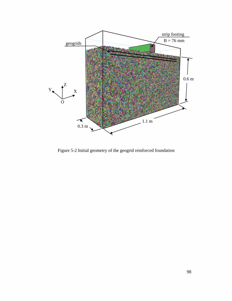
Figure 5-2 Initial geometry of the geogrid reinforced foundation
1.1 m 0.3 m
0.6 m
strip footing B = 76 mm geogrids
O
Z X Y
98
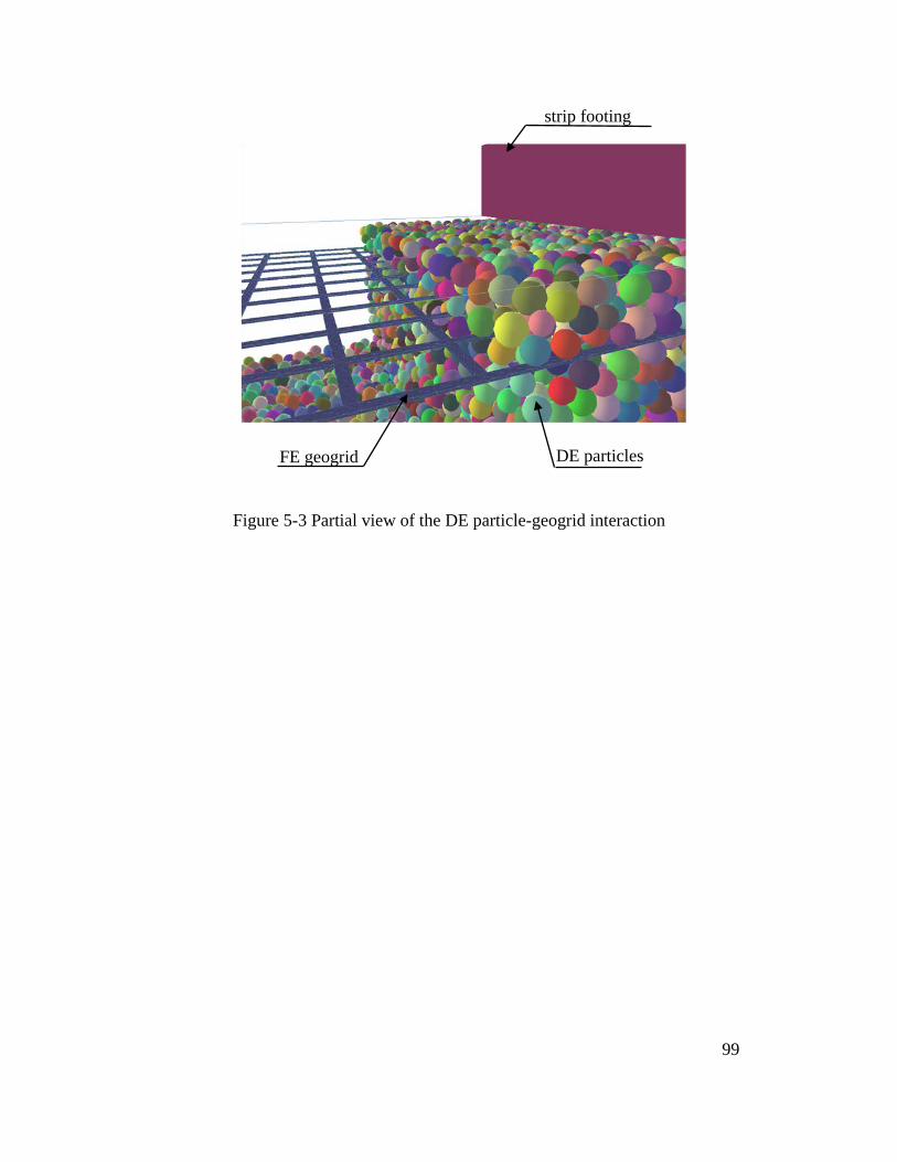
Figure 5-3 Partial view of the DE particle-geogrid interaction
strip footing
DE particles FE geogrid
99
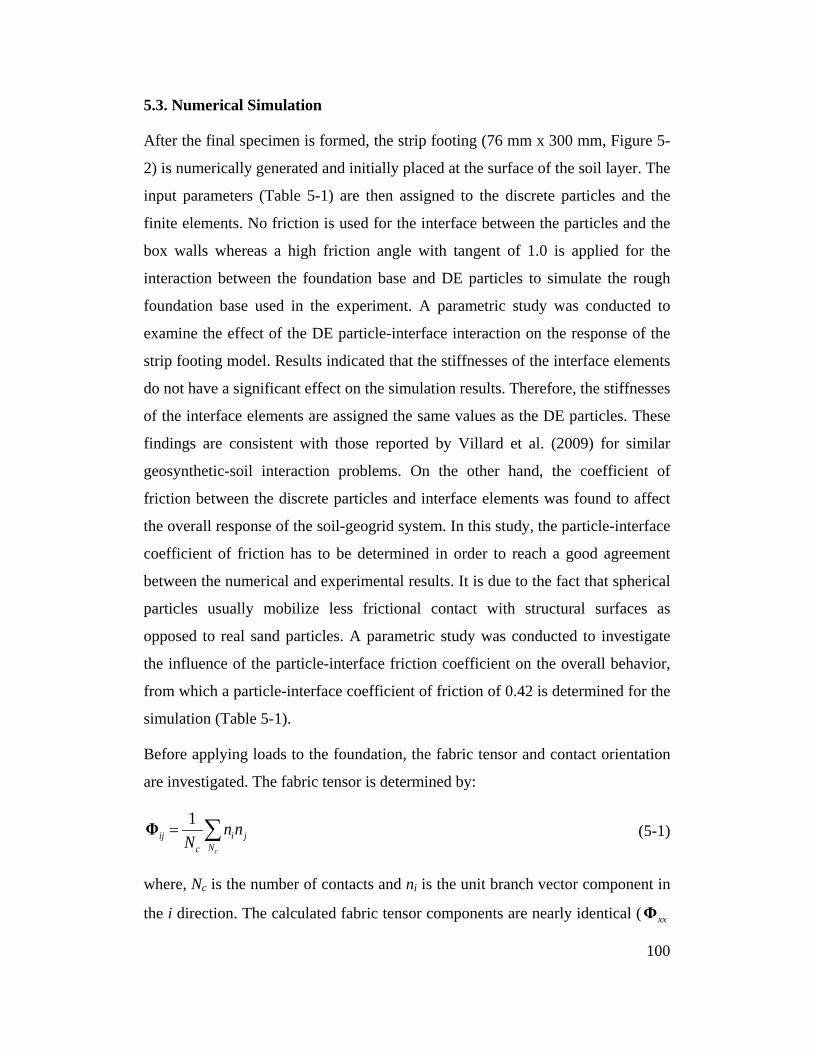
5.3. Numerical Simulation
After the final specimen is formed, the strip footing (76 mm x 300 mm, Figure 5-
2) is numerically generated and initially placed at the surface of the soil layer. The
input parameters (Table 5-1) are then assigned to the discrete particles and the
finite elements. No friction is used for the interface between the particles and the
box walls whereas a high friction angle with tangent of 1.0 is applied for the
interaction between the foundation base and DE particles to simulate the rough
foundation base used in the experiment. A parametric study was conducted to
examine the effect of the DE particle-interface interaction on the response of the
strip footing model. Results indicated that the stiffnesses of the interface elements
do not have a significant effect on the simulation results. Therefore, the stiffnesses
of the interface elements are assigned the same values as the DE particles. These
findings are consistent with those reported by Villard et al. (2009) for similar
geosynthetic-soil interaction problems. On the other hand, the coefficient of
friction between the discrete particles and interface elements was found to affect
the overall response of the soil-geogrid system. In this study, the particle-interface
coefficient of friction has to be determined in order to reach a good agreement
between the numerical and experimental results. It is due to the fact that spherical
particles usually mobilize less frictional contact with structural surfaces as
opposed to real sand particles. A parametric study was conducted to investigate
the influence of the particle-interface friction coefficient on the overall behavior,
from which a particle-interface coefficient of friction of 0.42 is determined for the
simulation (Table 5-1).
Before applying loads to the foundation, the fabric tensor and contact orientation
are investigated. The fabric tensor is determined by:
1
c
ij i jNc
n nN
= ∑Φ (5-1)
where, Nc is the number of contacts and ni is the unit branch vector component in
the i direction. The calculated fabric tensor components are nearly identical ( xxΦ
100
and yyΦ of about 0.33, zzΦ of about 0.34 where, z is the gravitational direction).
The distribution of contact orientation is shown in Figure 5-4. It can be seen that
the contacts are homogeneously distributed in all directions.
Following the above steps, the geogrids are then allowed to freely deform and
pressure at the foundation base is applied in small increments using a stress
control mechanism: for each loading stage, when the current pressure σ is
different from the target value vσ , the foundation moves vertically a distance of
( ) /vdz Kσ σ= − where, the stiffness K is determined by adding the normal
stiffnesses of all active particle-foundation base interactions. This mechanism
allows for a constant pressure to be maintained. Each load increment is kept
constant until convergence conditions are satisfied in both the DE and FE
domains. The foundation pressure is then increased for the next stage.
101
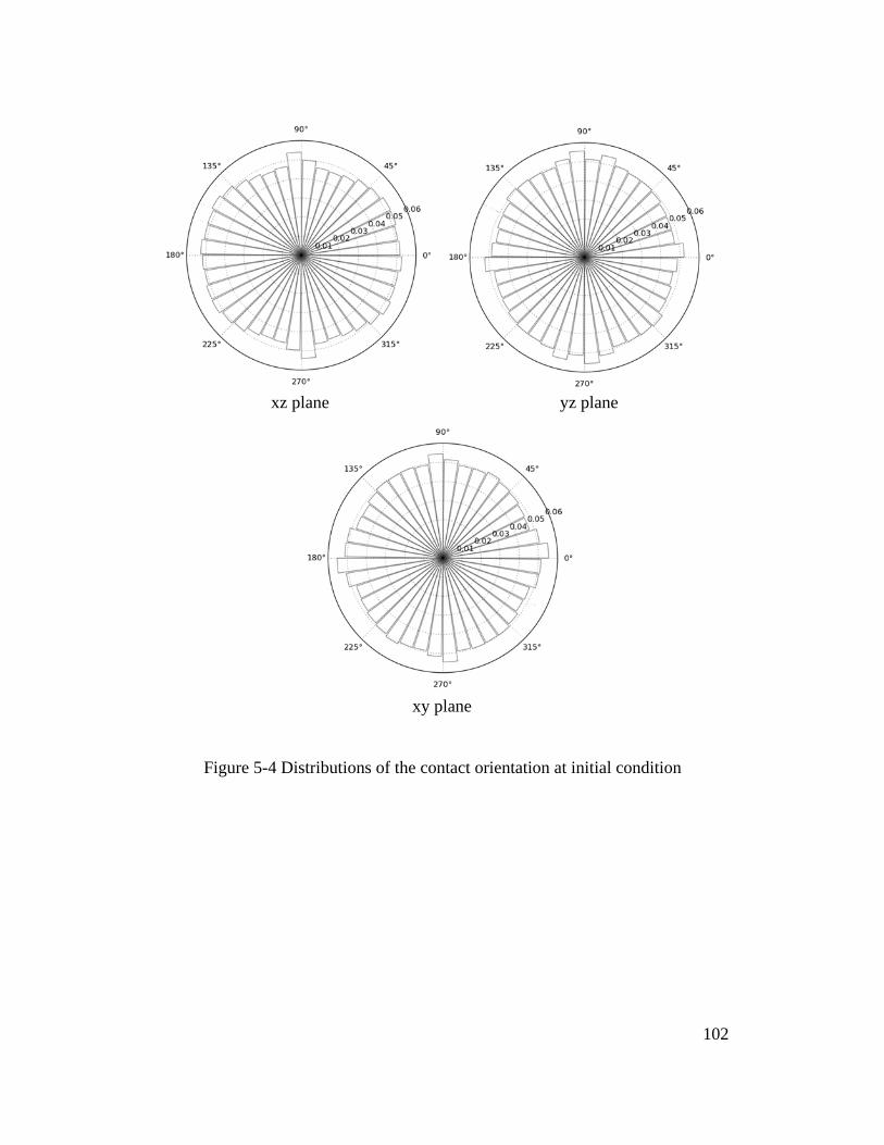
Figure 5-4 Distributions of the contact orientation at initial condition
xz plane yz plane
xy plane
102
5.4. Results and Discussions
5.4.1. Validation of the Numerical Model
In this section, the use of one or two geogrid sheets to reinforce the soil is
analyzed and compared to the case of no reinforcement. To validate the model,
the coupled FE-DE simulation results are first compared with the experimental
data. Figure 5-5 shows the relationship between the foundation pressure and
settlement for three cases: no reinforcement (N = 0), one geogrid layer (N = 1)
and two geogrid layers (N = 2). It can be seen that the numerical results agreed
well with the experimental data for all cases. For a given settlement, the load the
foundation can carry increased with the use of geogrid reinforcement. The
ultimate bearing capacity also increased with the number of geogrid layers (N). It
is also observed that the increase in the ultimate bearing capacity occurred with an
increase in the foundation settlement. The ultimate bearing capacity calculated by
Das et al. (1994) is consistent with the numerical results. This confirms the
agreement between the experiment and numerical simulations using the proposed
numerical framework.
5.4.2. Response of the Geogrids
The deformed shapes of the geogrid layers for a foundation pressure q = 125 kPa
are shown in Figure 5-6. The vertical displacement of the geogrid for one
reinforcement layer (N = 1) is shown in Figure 5-6a whereas the case of two
geogrid layers (N = 2) is shown in Figure 5-6b. It can be seen that the vertical
displacement of the geogrid for N = 1 is generally larger than that for N = 2. In
addition, the vertical displacement of the upper geogrid sheet is larger than that of
the lower one. Consistent with the displacement pattern, the tensile stresses in the
geogrid for N = 1 were found to be larger than that for N = 2 (Figure 5-7). It is
also noted that the upper geogrid layer experienced higher tensile stresses than the
lower layer. In both cases, the deformations of the geogrids occurred mainly in a
region below the foundation and very small deformations were observed outside
that region. The stresses Sxx were highest below the foundation and decreased
103
with distance from the loading area. The vertical displacement and tensile stress
distributions of the geogrid for N = 1 are shown in Figure 5-8. It can be seen that
the vertical displacements and tensile stresses of the geogrid occurred within a
distance of 1.5B from the foundation center and became negligible outside this
region. The maximum calculated vertical displacements and tensile stresses in the
geogrid for different footing pressures are shown in Figure 5-9. It is observed that
for a given pressure, the vertical displacements and tensile stresses in the geogrid
were larger for N = 1 than for N = 2. It is also noted from Figure 5-9a and 5-9b
that the deformation and tensile stresses of the upper geogrid layer were generally
larger than the lower one for N = 2.
104
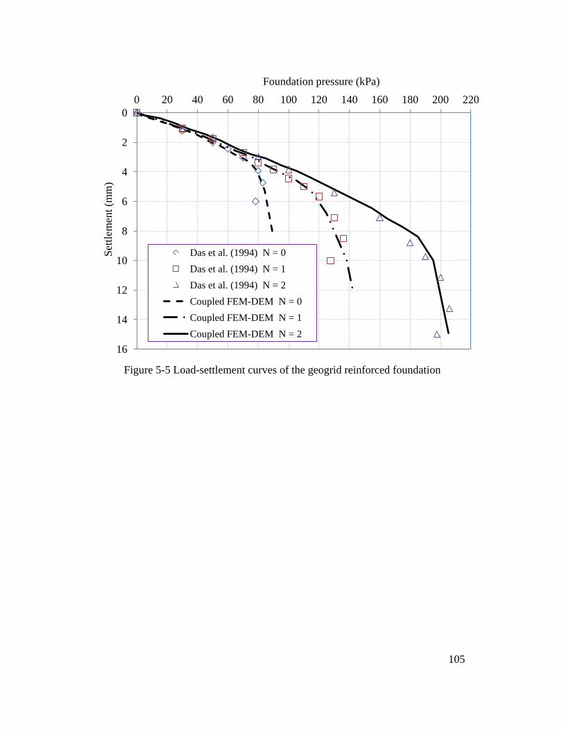
Figure 5-5 Load-settlement curves of the geogrid reinforced foundation
0
2
4
6
8
10
12
14
16
0 20 40 60 80 100 120 140 160 180 200 220 Se
ttlem
ent (
mm
)
Foundation pressure (kPa)
Das et al. (1994) N = 0 Das et al. (1994) N = 1 Das et al. (1994) N = 2 Coupled FEM-DEM N = 0 Coupled FEM-DEM N = 1 Coupled FEM-DEM N = 2
105
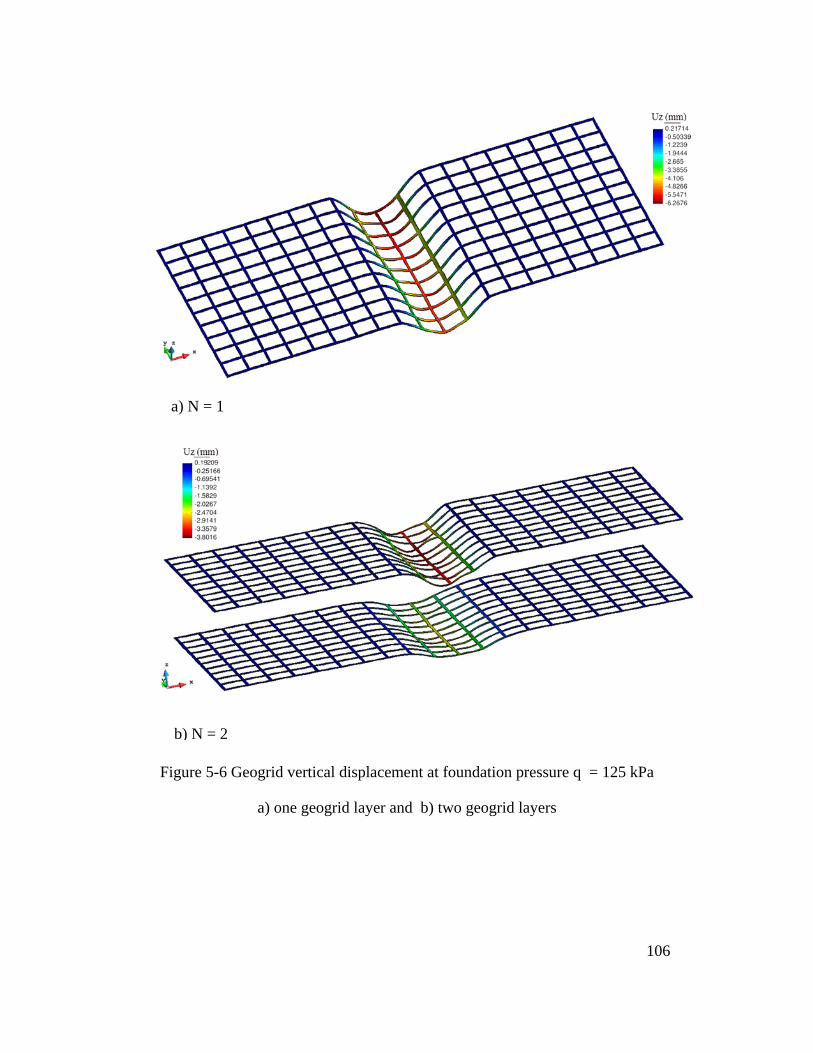
Figure 5-6 Geogrid vertical displacement at foundation pressure q = 125 kPa
a) one geogrid layer and b) two geogrid layers
b) N = 2
a) N = 1
106
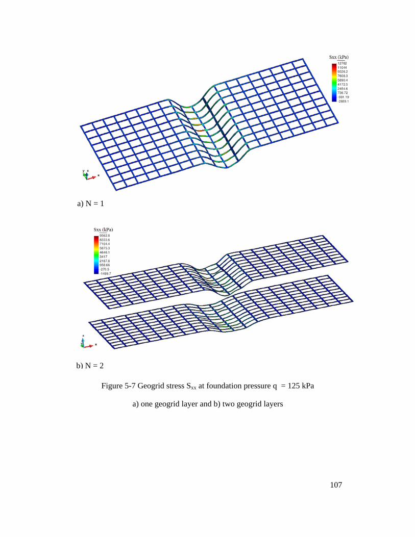
Figure 5-7 Geogrid stress Sxx at foundation pressure q = 125 kPa
a) one geogrid layer and b) two geogrid layers
b) N = 2
a) N = 1
107
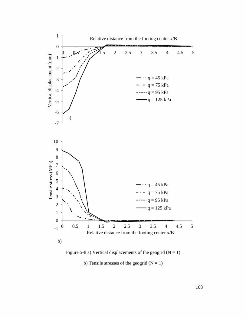
Figure 5-8 a) Vertical displacements of the geogrid (N = 1)
b) Tensile stresses of the geogrid (N = 1)
-7
-6
-5
-4
-3
-2
-1
0
1
0 0.5 1 1.5 2 2.5 3 3.5 4 4.5 5 Ve
rtica
l dis
plac
emen
t (m
m)
Relative distance from the footing center x/B
q = 45 kPa q = 75 kPa q = 95 kPa q = 125 kPa
a)
-1 0 1 2 3 4 5 6 7 8 9
10
0 0.5 1 1.5 2 2.5 3 3.5 4 4.5 5
Tens
ile st
ress
(MPa
)
Relative distance from the footing center x/B
q = 45 kPa q = 75 kPa q = 95 kPa q = 125 kPa
b)
108
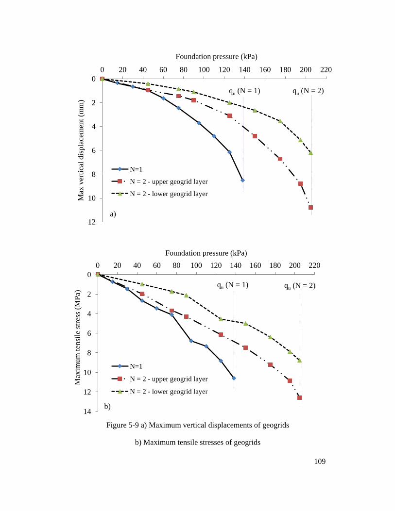
Figure 5-9 a) Maximum vertical displacements of geogrids
b) Maximum tensile stresses of geogrids
0
2
4
6
8
10
12
0 20 40 60 80 100 120 140 160 180 200 220 M
ax v
ertic
al d
ispl
acem
ent (
mm
)
Foundation pressure (kPa)
N=1
N = 2 - upper geogrid layer
N = 2 - lower geogrid layer
a)
qu (N = 1) qu (N = 2)
0
2
4
6
8
10
12
14
0 20 40 60 80 100 120 140 160 180 200 220
Max
imum
tens
ile st
ress
(MPa
)
Foundation pressure (kPa)
N=1
N = 2 - upper geogrid layer
N = 2 - lower geogrid layer
b)
qu (N = 1) qu (N = 2)
109
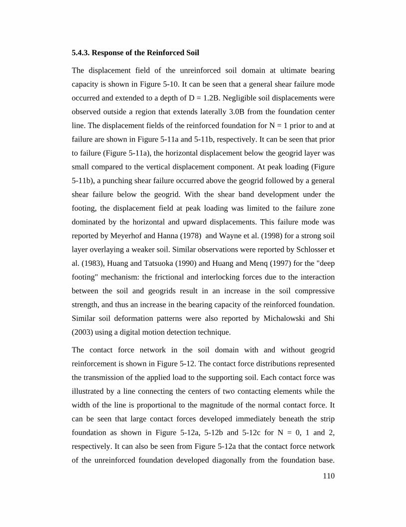
5.4.3. Response of the Reinforced Soil
The displacement field of the unreinforced soil domain at ultimate bearing
capacity is shown in Figure 5-10. It can be seen that a general shear failure mode
occurred and extended to a depth of D = 1.2B. Negligible soil displacements were
observed outside a region that extends laterally 3.0B from the foundation center
line. The displacement fields of the reinforced foundation for N = 1 prior to and at
failure are shown in Figure 5-11a and 5-11b, respectively. It can be seen that prior
to failure (Figure 5-11a), the horizontal displacement below the geogrid layer was
small compared to the vertical displacement component. At peak loading (Figure
5-11b), a punching shear failure occurred above the geogrid followed by a general
shear failure below the geogrid. With the shear band development under the
footing, the displacement field at peak loading was limited to the failure zone
dominated by the horizontal and upward displacements. This failure mode was
reported by Meyerhof and Hanna (1978) and Wayne et al. (1998) for a strong soil
layer overlaying a weaker soil. Similar observations were reported by Schlosser et
al. (1983), Huang and Tatsuoka (1990) and Huang and Menq (1997) for the "deep
footing" mechanism: the frictional and interlocking forces due to the interaction
between the soil and geogrids result in an increase in the soil compressive
strength, and thus an increase in the bearing capacity of the reinforced foundation.
Similar soil deformation patterns were also reported by Michalowski and Shi
(2003) using a digital motion detection technique.
The contact force network in the soil domain with and without geogrid
reinforcement is shown in Figure 5-12. The contact force distributions represented
the transmission of the applied load to the supporting soil. Each contact force was
illustrated by a line connecting the centers of two contacting elements while the
width of the line is proportional to the magnitude of the normal contact force. It
can be seen that large contact forces developed immediately beneath the strip
foundation as shown in Figure 5-12a, 5-12b and 5-12c for N = 0, 1 and 2,
respectively. It can also be seen from Figure 5-12a that the contact force network
of the unreinforced foundation developed diagonally from the foundation base.
110
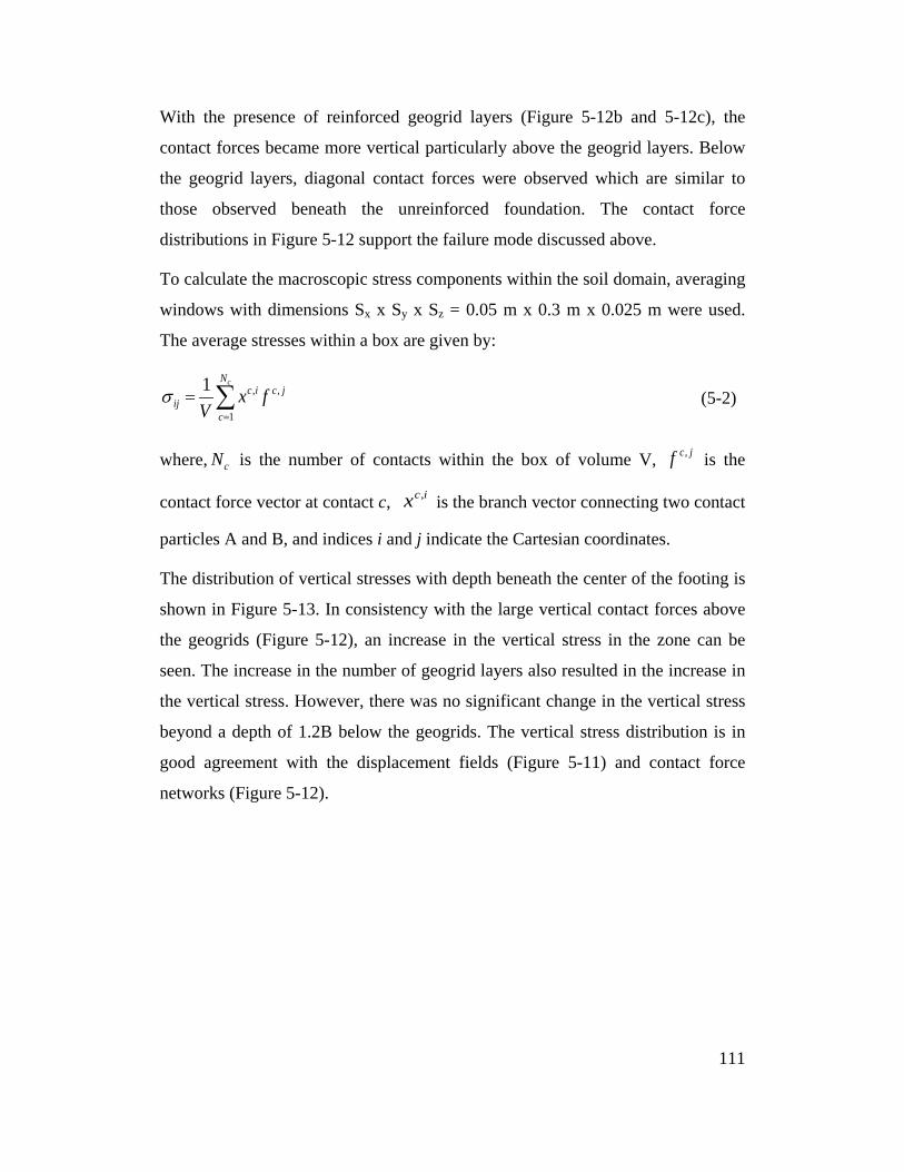
With the presence of reinforced geogrid layers (Figure 5-12b and 5-12c), the
contact forces became more vertical particularly above the geogrid layers. Below
the geogrid layers, diagonal contact forces were observed which are similar to
those observed beneath the unreinforced foundation. The contact force
distributions in Figure 5-12 support the failure mode discussed above.
To calculate the macroscopic stress components within the soil domain, averaging
windows with dimensions Sx x Sy x Sz = 0.05 m x 0.3 m x 0.025 m were used.
The average stresses within a box are given by:
, ,
1
1 cNc i c j
ijc
x fV
σ=
= ∑ (5-2)
where, cN is the number of contacts within the box of volume V, jcf , is the
contact force vector at contact c, icx , is the branch vector connecting two contact
particles A and B, and indices i and j indicate the Cartesian coordinates.
The distribution of vertical stresses with depth beneath the center of the footing is
shown in Figure 5-13. In consistency with the large vertical contact forces above
the geogrids (Figure 5-12), an increase in the vertical stress in the zone can be
seen. The increase in the number of geogrid layers also resulted in the increase in
the vertical stress. However, there was no significant change in the vertical stress
beyond a depth of 1.2B below the geogrids. The vertical stress distribution is in
good agreement with the displacement fields (Figure 5-11) and contact force
networks (Figure 5-12).
111
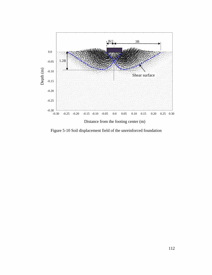
Figure 5-10 Soil displacement field of the unreinforced foundation
-0.30 -0.25 -0.20 -0.15 -0.10 -0.05 0.0 0.05 0.10 0.15 0.20 0.25 0.30
Distance from the footing center (m)
0.0
-0.05
-0.10
-0.15
-0.20
-0.25
-0.30
Dep
th (m
)
3B
1.2B
B/2
Shear surface
112
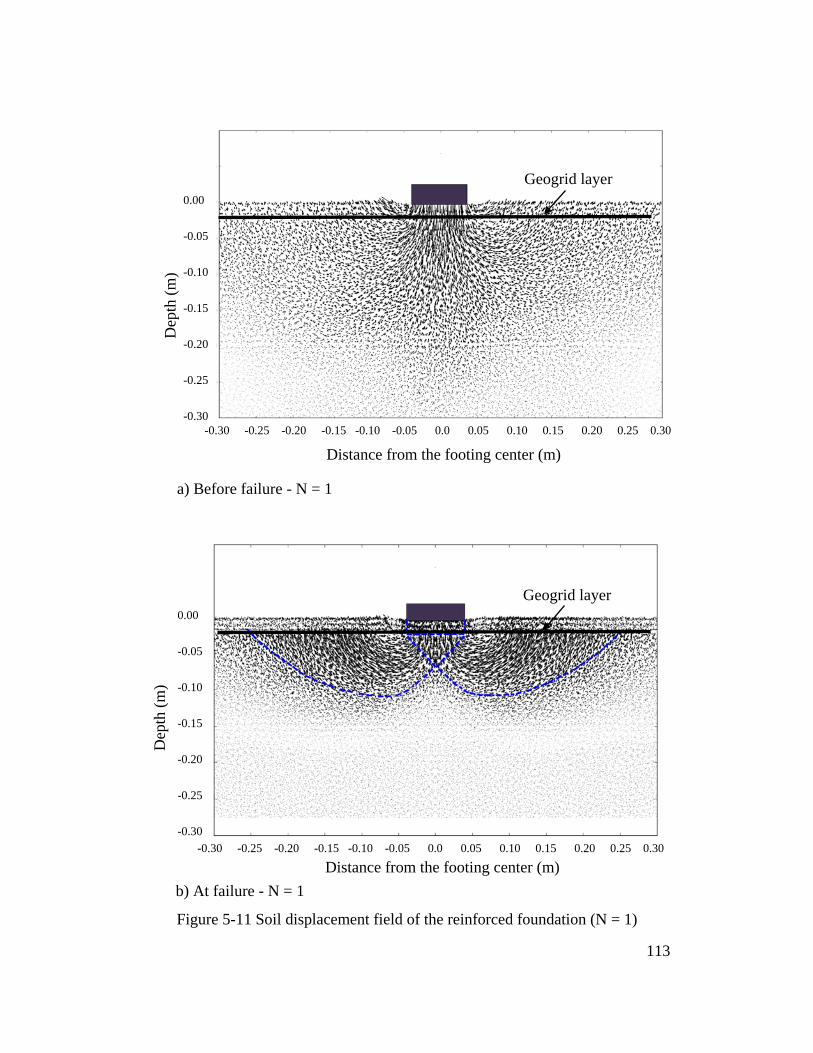
Figure 5-11 Soil displacement field of the reinforced foundation (N = 1)
-0.30 -0.25 -0.20 -0.15 -0.10 -0.05 0.0 0.05 0.10 0.15 0.20 0.25 0.30
Distance from the footing center (m)
0.00
-0.05
-0.10
-0.15
-0.20
-0.25
-0.30
Dep
th (m
)
Geogrid layer
b) At failure - N = 1
-0.30 -0.25 -0.20 -0.15 -0.10 -0.05 0.0 0.05 0.10 0.15 0.20 0.25 0.30
Distance from the footing center (m)
0.00
-0.05
-0.10
-0.15
-0.20
-0.25
-0.30
Dep
th (m
)
Geogrid layer
a) Before failure - N = 1
113
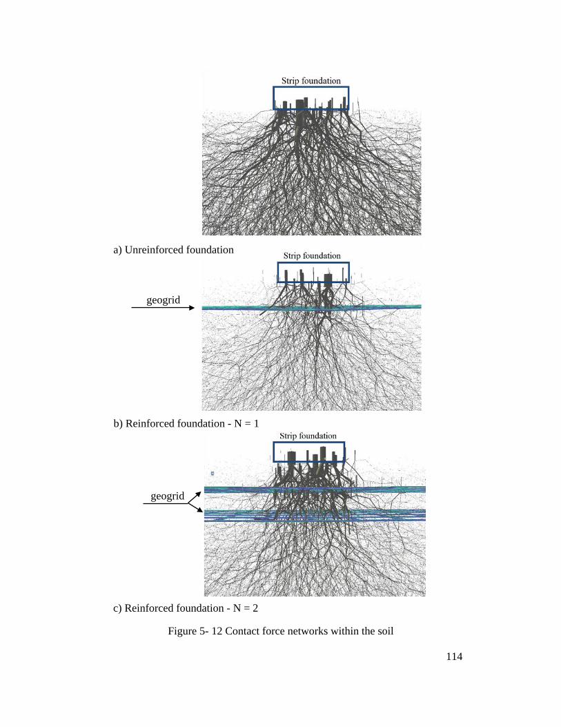
Figure 5- 12 Contact force networks within the soil
a) Unreinforced foundation
b) Reinforced foundation - N = 1
geogrid
geogrid
c) Reinforced foundation - N = 2
114
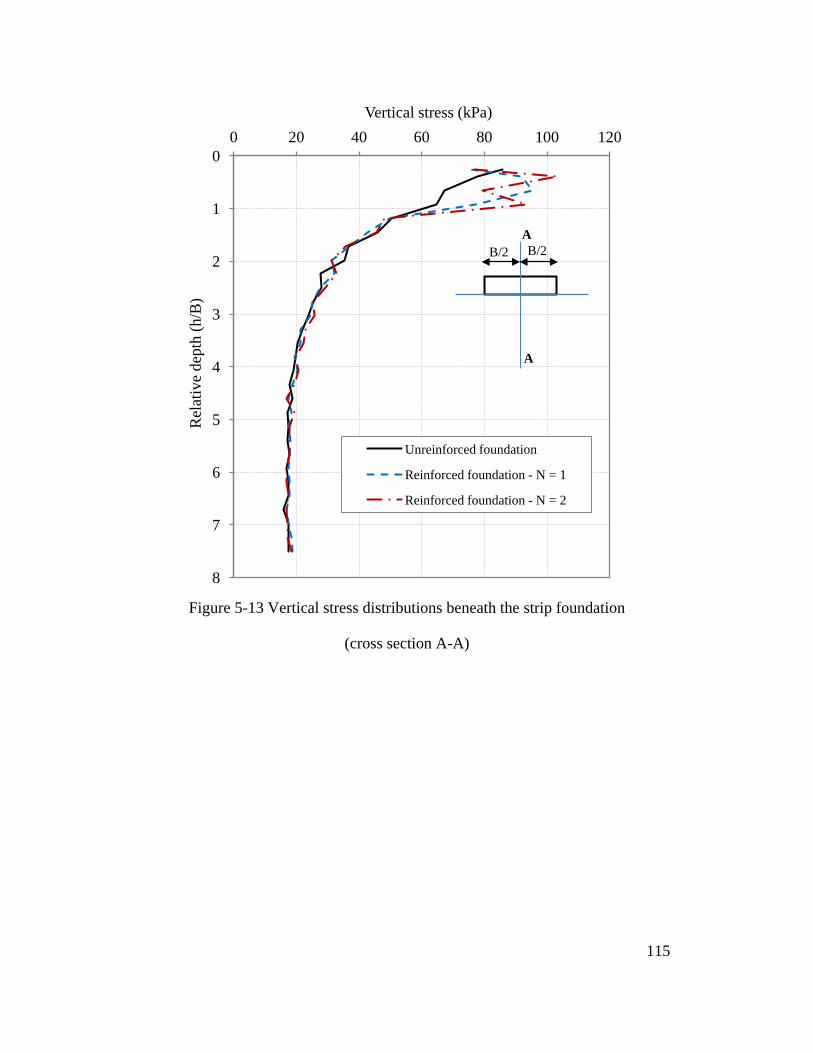
Figure 5-13 Vertical stress distributions beneath the strip foundation
(cross section A-A)
0
1
2
3
4
5
6
7
8
0 20 40 60 80 100 120
Rel
ativ
e de
pth
(h/B
)
Vertical stress (kPa)
Unreinforced foundation
Reinforced foundation - N = 1
Reinforced foundation - N = 2
B/2 B/2 A
A
115
5.5. Summary and Conclusions
This study investigated soil-geogrid interaction using a coupled FE-DE
framework. The soil was modeled using DE while the geogrid was modeled using
FE. The interaction between the DE and FE domains was ensured by using
interface elements. The developed framework was used to investigate the
behavior of strip foundation over geogrid reinforced sand. The soil-geogrid
interlocking effect was demonstrated. The 3D geometry of the geogrid, its
deformation and stress distribution were represented. The microscopic behavior of
the soil domain relative to soil displacements, contact orientations, contact forces
were also analyzed.
The numerical modeling of the geogrid reinforced strip foundation provided a
very good agreement with the experimental results. Increasing the number of
geogrid layers resulted in an increase of the ultimate bearing capacity. Geogrid
deformations and tensile stresses for N = 1 were larger than those for N = 2.
When two layers of geogrid were used, the upper layer was subjected to larger
deformations and tensile stresses than the lower layer. At the ultimate load, a
punching shear failure occurred above the geogrid followed by a general shear
failure below the geogrid. The use of geogrid reinforcement also resulted in an
increase in the vertical stresses in the soil.
The proposed coupled FE-DE method has proven to be effective in capturing soil-
geogrid interaction and analyzing the behavior of both geogrid and surrounding
material.
116
Preface to Chapter 6
The efficiency of the coupled Finite-Discrete element framework in analyzing
soil-structure interaction problems has been demonstrated in the previous
chapters: geogrid pullout test (Chapter 4) and geogrid reinforced strip foundation
(Chapter 5). A different soil reinforcement problem, which is geogrid-reinforced
fill over void, is analyzed in this chapter as an example of a condition where soil
below the reinforced layers experiences large vertical deformation. The
microscopic behavior of the fill overlying void with and without geogrid
reinforcement is investigated. The efficiency of the developed coupled program in
such challenging condition is therefore demonstrated.
117
CHAPTER 6
Three-Dimensional Analysis of Geogrid Reinforced Fill over Void Using Finite-Discrete Element Framework *
Abstract
Three-dimensional analysis of soil-structure interaction problems considering the
detailed response at the particle scale level is a challenging numerical modeling
problem. An efficient numerical framework that takes advantage of both the finite
and discrete element approaches to investigate soil-geogrid interaction is
described in this paper. The method uses finite elements to model the structural
components and discrete particles to model the surrounding soil to reflect the
discontinuous nature of the granular material. The coupled framework is used to
investigate the behavior of geogrid-reinforced fill over strong formation
containing void. The numerical results provide a new insight into the nature of the
three-dimensional interaction between the soil and the geogrid.
Keywords: geogrid reinforcement, finite-discrete element, fill system over void,
numerical simulation.
* A version of this chapter has been submitted to International Journal of
Geomechanics ASCE, 2013.
118
6.1. Introduction
Fill structures such as embankments and highways are often constructed on
natural ground. Although site investigation is usually performed before the design
process, it is possible that existing voids are not detected or cavities may develop
during the service life of the fill. Cavities are common in coral and karstic
formations or in rock with soft inclusions (Agaiby and Jones, 1995). These voids
can collapse and cause severe damage to structures in their vicinity. This problem
was first studied by Terzaghi (1936). A trap door at the base of a soil-filled
container was lowered causing the soil to move into the generated void. The trap
door problem was also modeled numerically by Koutsabeloulis and Grifiths
(1989) using the FEM. One method to protect the surface structure over voids is
using reinforcement beneath the foundation of the structure. Reinforcement that
bridges over voids reduces settlements and protects the structures from failure.
Kinney and Connor (1987) conducted field tests to investigate the performance of
road embankments over voids. Results suggested that geosynthetics can be
beneficial when a fill is placed over voids. The ability of geogrid reinforced
pavements to provide an early warning system of a void beneath a road was
reported by Bridle et al. (1994). The efficiency of reinforcement in road
applications was also reported by Villard et. al (2000). Analytical solutions for
reinforced systems over voids have been reported by Giroud et al. (1990),
Poorooshasb (1991), Agaiby and Jones (1995), Wang et al. (1996), Villard et al.
(2000) and Briançon and Villard (2008). FE modeling of the reinforced systems
has been reported by Gabr et al. (1992), Gabr and Hunter (1994), Lawson et al.
(1994), Agaiby and Jones (1995) and Gaetano (2010). In most cases, only 2D
models were used and the 3D geometry of the geosynthetics was not represented.
DE modeling of similar problems such as geogrid-reinforced embankments over
piles (Han et al., 2011) did not consider the 3D geogrid geometry. However,
Bridle et al. (1994) shown that interlocking mechanism generates a stiffened
granular layer which prevents collapse into the void. A simplified 2D model of
the geogrid geometry, may therefore, misrepresent the behavior of the reinforced
119
earth structures. In this study, a fill on a geogrid layer overlying a void is
simulated using the coupled FE-DE framework. The proposed framework is
capable of representing the 3D geometry of the geogrid and the interlocking
mechanism associated with the soil-geogrid interaction.
6.2. Model Generation
A granular fill layer reinforced with a geogrid layer overlying a void is analyzed
in this section using the proposed coupled FE-DE framework. While cavities may
not be always detected during geophysical investigation, the presence of these
cavities can have a negative impact on overlying structures such as highway
embankments. The numerical analysis aims at investigating the soil-geogrid
interaction mechanism and the behavior of the geogrid and supported soil with the
presence of small subsurface voids. In this study, a fill layer with a thickness 0.6m
constructed over a natural soil formation experiencing the development of a
sudden cavity (width 0.2m and height 0.3m) is simulated (Figure 6-1). It is
assumed that the void develops in a rigid formation layer and is infinitely long in
the out-of-plane direction. Previous studies (Giroud et al., 1990;
Poorooshasb,1991; Agaiby and Jones, 1995; Wang et al., 1996, Villard et al.,
2000; Briançon and Villard, 2008) generally assumed the geosynthetics layers are
installed right above the rigid surface. This assumption simplifies the analysis
however it does not always represent the case when a natural soil formation
overlies bedrock in which voids develop. In this study, both cases have been
studied using the coupled FE-DE method. The geogrid is simulated using FE
while the fill (and the underlying soil) is simulated using DE whereas the rigid
formation is modeled as non-deformable FE domain. The placement of the
geogrid directly on the rigid formation was found to cause numerical instability in
the model unless additional restraints are applied to the geogrid. These restraints
affect the soil-geogrid frictional resistance and interlocking effect as they prevent
the geogrid from deforming laterally. To ensure proper interaction between the
geogrid and soil, the geogrid is installed over a thin soil layer of thickness 0.1m
overlying the non-deformable foundation as shown in Figure 6-1. The geogrid is
120
assumed to be installed on the natural soil surface prior to the construction of the
fill. A surcharge of 5kN/m2 is applied on top of the fill to simulate surface
loading. This surcharge is modeled using a DE layer of thickness 0.05m placed on
top of the fill with high density particles. The cavity is assumed to develop after
the fill has been constructed.
6.3. Numerical Simulation
The soil properties used in the previous reinforced foundation problem in Chapter
5 are used for the fill material (Table 6-1). The properties of the natural soil and
the fill are assumed to be the same for the purpose of simplification. The geogrid
type (Tensar SS-0) from the previous reinforced foundation experiment (Chapter
5) is also used for the reinforcement. Parametric studies show that a void width of
0.2m results in negligible deformations of the soil and geogrid outside a region
0.45 m from the void center line. Therefore, an assemblage of particles with a
length 1.1m is appropriate to represent the soil domain. The numerical geogrid
has a length of 1.1 m and a width of 0.3m which represents the placement of the
reinforcement over the soil layer (Figure 6-2).
The assembly is generated using the multi-layer packing process mentioned
previously. The rigid formation is first modeled using non-deformable FE
elements without voids. The natural soil layer of thickness 0.1m is then generated
followed by the generation of the geogrid layer. The fill is then generated in
layers until the target thickness of 0.6 m is achieved. A surcharge of 5kN/m2 is
applied on top of the fill by generating a 0.05 m thick layer of high density
particles. The final assemblage consists of over 280,000 DE particles and 2800 FE
elements. After material properties have been assigned to all FE and DE elements,
the geogrid is allowed to freely deform. The initial condition of the soil
assemblage is achieved when the convergence conditions are satisfied (all internal
and external forces are balanced). The FE elements in the void location are then
removed to numerically simulate the development of the void.
121

Table 6-1 Input parameters for the simulation
Type of elements Parameter Value
Discrete particles Density (kg/m3) 2650
Material modulus E (MPa) 38
Ratio KT/KN 0.25
Coefficient of friction (tanϕ ) 0.68
rβ 0.01
rη 1.0
Damping coefficient 0.2
Finite elements Young modulus E (MPa) 1.4E+3
Poisson's ratio ν 0.3
Interface elements Material modulus E (MPa) 38
Ratio KT/KN 0.25
Coefficient of friction (tanϕ ) 0.42
122
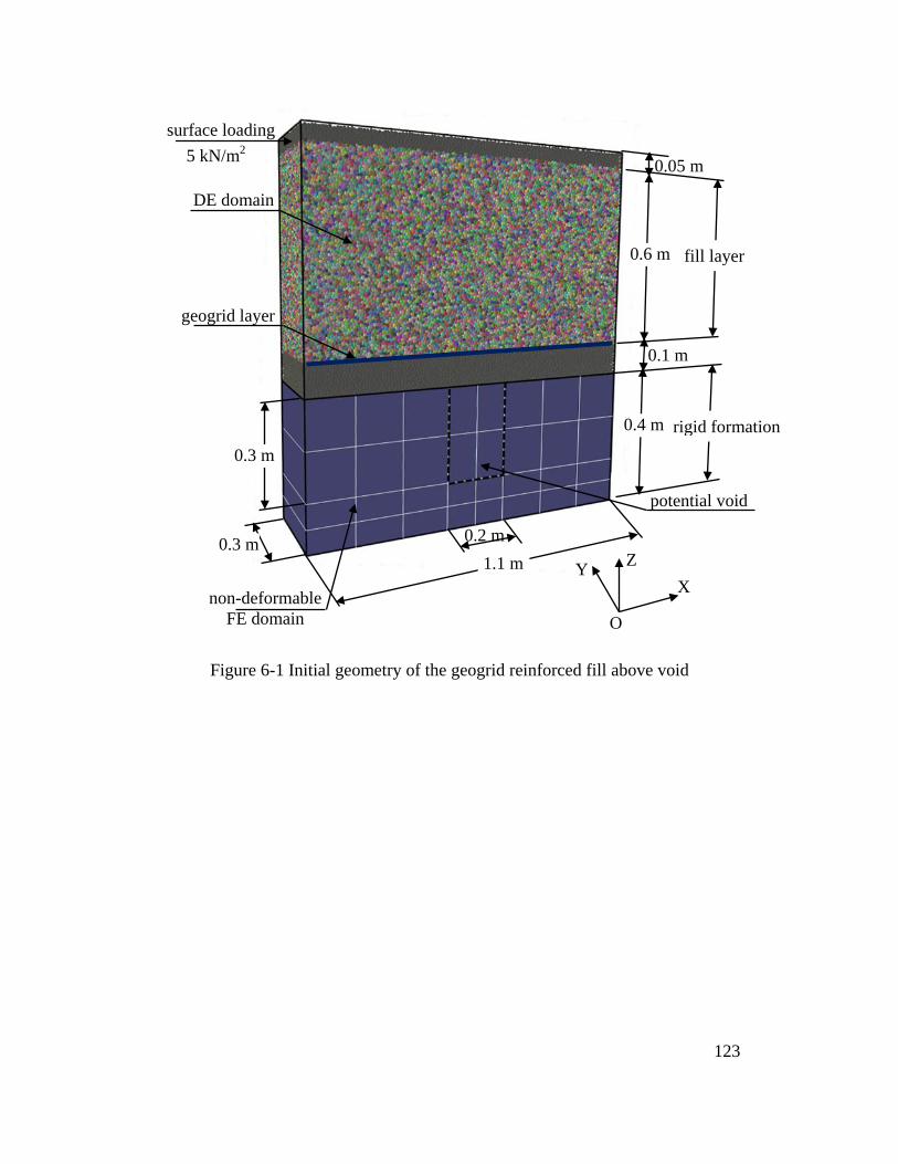
Figure 6-1 Initial geometry of the geogrid reinforced fill above void
1.1 m 0.3 m
0.4 m
0.2 m
0.3 m
non-deformable FE domain
DE domain
X Z Y
O
geogrid layer
potential void
surface loading 5 kN/m2 0.05 m
0.1 m
rigid formation
0.6 m fill layer
123
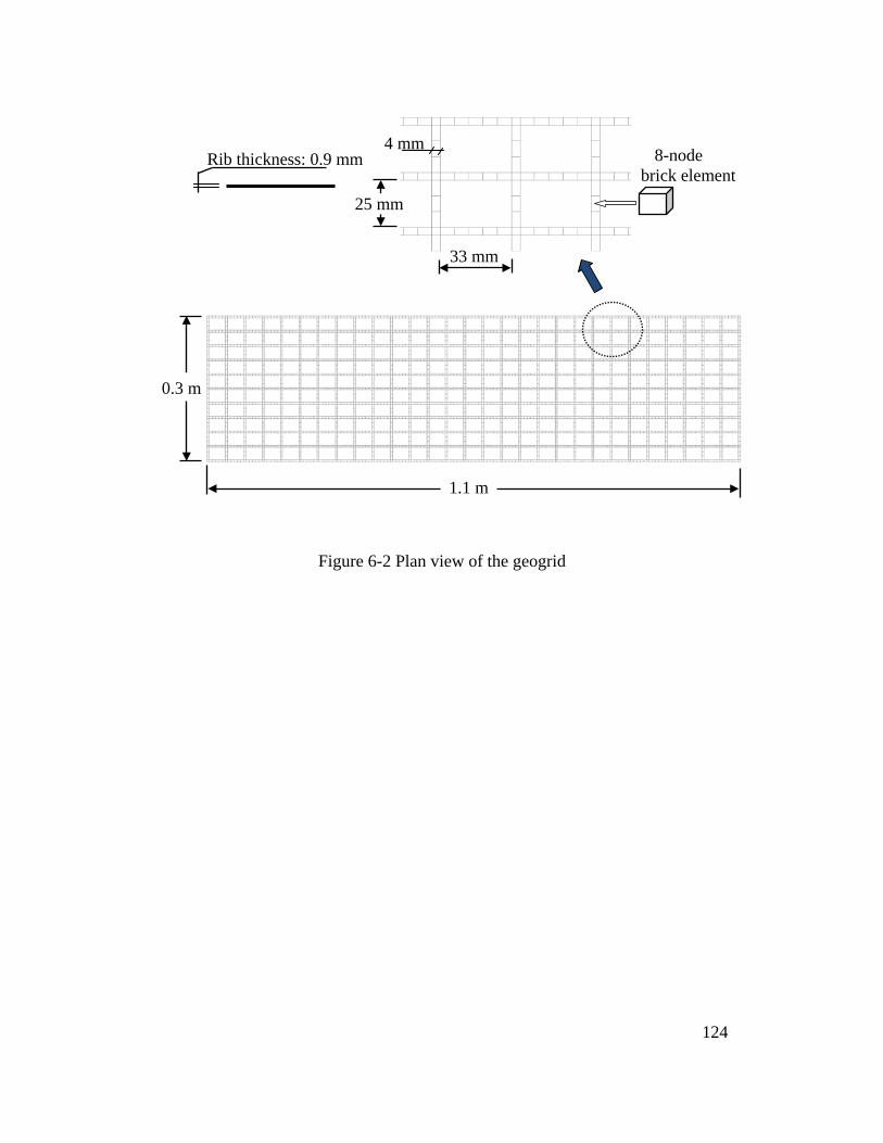
Figure 6-2 Plan view of the geogrid
1.1 m
0.3 m
33 mm
25 mm
4 mm Rib thickness: 0.9 mm 8-node
brick element
124
6.4. Results and Discussions
6.4.1. Response of the Geogrid
The deformed shape of the geogrid is shown in Figure 6-3. The largest
deformations and tensile stresses were observed in a region above the void. Due
to the soil movement toward the void, the geogrid deformed and tensile stress in
the geogrid developed to balance the loads acting on the geogrid sheet.
Distributions of the vertical displacements and tensile stresses along the geogrid
are shown in Figure 6-4. It can be seen that the vertical displacements and tensile
stresses were small near the two geogrid ends and largest at the geogrid center.
The interlocking and frictional contact forces contribute to the anchoring
mechanism. To examine the importance of the interlocking effect, a parametric
study has been performed by reducing the friction coefficient between the soil and
geogrid. It was found that when the interface friction coefficient is reduced to
zero, the geogrid anchoring is still ensured with a small increase in the geogrid
vertical displacement. This demonstrates the dominant role of the interlocking
effect in the geogrid anchoring mechanism. A similar observation on the
importance of the geogrid interlocking effect was reported by Bridle et al. (1994).
The feasibility of the coupled FE-DE framework to model the interlocking effect
is therefore verified.
6.4.2. Response of the Reinforced Soil
The displacement fields of the fill layer without and with geogrid reinforcement
are shown in Figure 6-5. In the case of unreinforced fill (Figure 6-5a), downward
soil movement developed above the void location. However, soil collapse at the
fill surface did not occur and the fill stability was achieved due to soil arching
over the void. Figure 6-5b shows the displacement field of the geogrid reinforced
fill. It can be seen that soil displacements above the geogrid layer were much
smaller compared to the unreinforced fill and the geogrid efficiently prevented the
soil from moving toward the void. This demonstrates the efficiency of the
125
interlocking effect in generating a stiffened granular layer above the geogrid
(Bridle et al., 1994).
The contact orientations in the unreinforced fill are shown in Figure 6-6. It can be
seen that with the development of the soil arching within the fill, more contacts
were seen in the x direction than in the z direction (xz plane view). This strong
anisotropy induced by the soil arching which demonstrated a stronger contact
orientation in the horizontal direction than in the vertical direction. The
distribution of contacts in the yz plane was elliptical, with the z component being
slightly larger than the y component. Meanwhile, quite uniform distribution of the
contact orientation was observed in the xy plane. With the placement of a geogrid
layer above the void, the distribution of contact orientations in the xz plane of the
reinforced fill (Figure 6-7) showed less arching with only a slightly larger value in
the horizontal direction compared to the vertical direction. Uniform contact
distributions in the yz and xy planes were also observed. The geogrid
reinforcement prevents the rearrangement of contact forces compared to the
unreinforced fill with the creation of a void.
The soil deformation in the fill layer can also be evaluated by analyzing the
change in porosity in the soil domain. Using the DE analysis, the change of
porosity is obtained by comparing the change in the volume of DE particles
within a given volume of dimensions Sx x Sy x Sz = 0.1 m x 0.3 m x 0.1m. The
changes in porosity without and with the geogrid reinforcement are shown in
Figure 6-8a and 6-8b, respectively. In both cases, there was an increase in
porosity corresponding to the volumetric dilation in the fill. Maximum dilations
occurred above the void location. Up to 10% of porosity changes were observed
in the unreinforced fill while much smaller changes (less than 1.1%) were
observed in the geogrid reinforced fill. The volumetric dilation in the fill was also
reported by Costa et al. (2009) and Han et al. (2011).
Soil arching development results in the stress redistribution within the soil mass.
Average stresses in the fill were calculated with boxes with dimensions Sx x Sy x
126
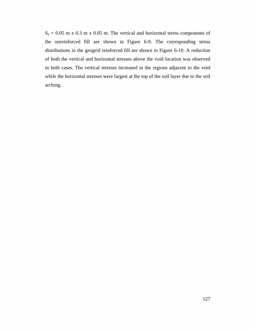
Sz = 0.05 m x 0.3 m x 0.05 m. The vertical and horizontal stress components of
the unreinforced fill are shown in Figure 6-9. The corresponding stress
distributions in the geogrid reinforced fill are shown in Figure 6-10. A reduction
of both the vertical and horizontal stresses above the void location was observed
in both cases. The vertical stresses increased in the regions adjacent to the void
while the horizontal stresses were largest at the top of the soil layer due to the soil
arching.
127
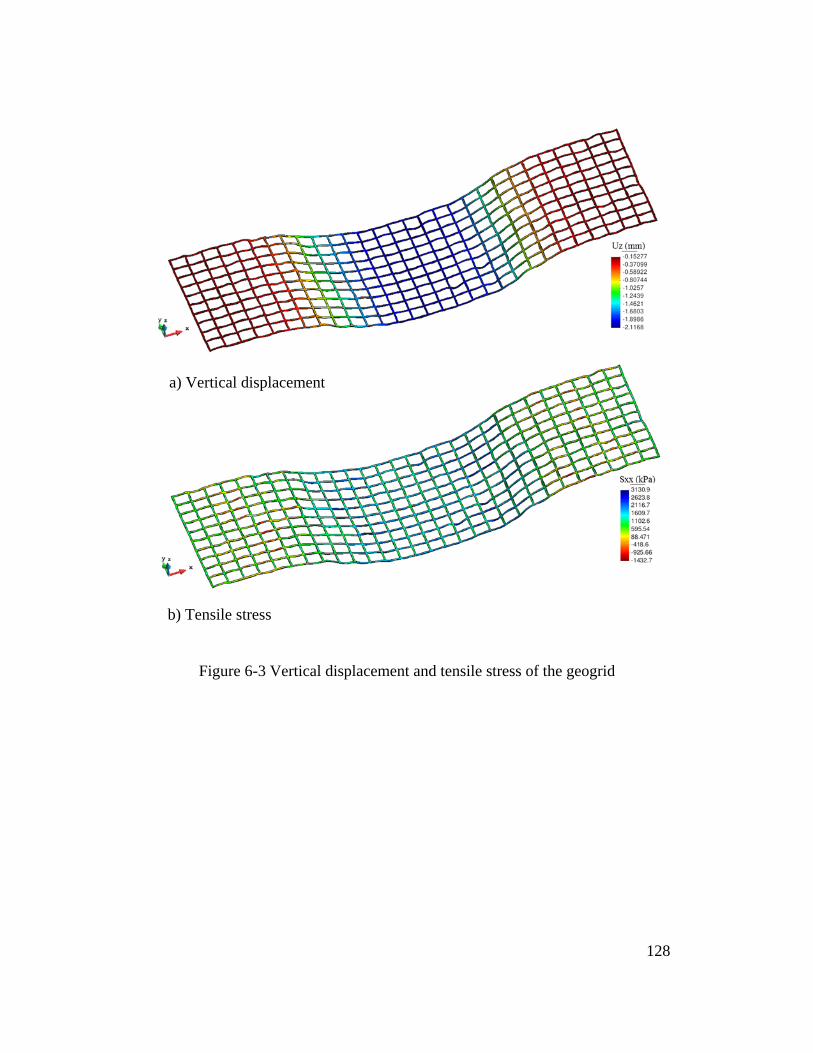
Figure 6-3 Vertical displacement and tensile stress of the geogrid
a) Vertical displacement
b) Tensile stress
128
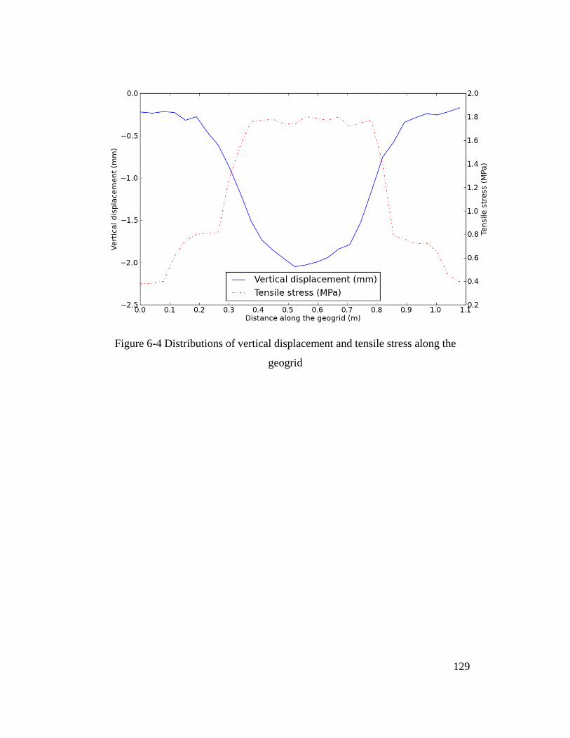
Figure 6-4 Distributions of vertical displacement and tensile stress along the
geogrid
129
Figure 6-5 Soil displacement fields
0.0 0.1 0.2 0.3 0.4 0.5 0.6 0.7 0.8 0.9 1.0 1.1
0.0 0.1 0.2 0.3 0.4 0.5 0.6 0.7 0.8 0.9 1.0 1.1
Distance (m)
Distance (m)
0.0
-0.1
-0.2
-0.3
-0.4
-0.5
-0.6
-0.7
-0.8
Dep
th (m
)
0.0
-0.1
-0.2
-0.3
-0.4
-0.5
-0.6
-0.7
-0.8
Dep
th (m
)
void
FE domain
FE domain
FE domain
FE domain
void
geogrid layer
a) Unreinforced fill
b) Reinforced fill
130
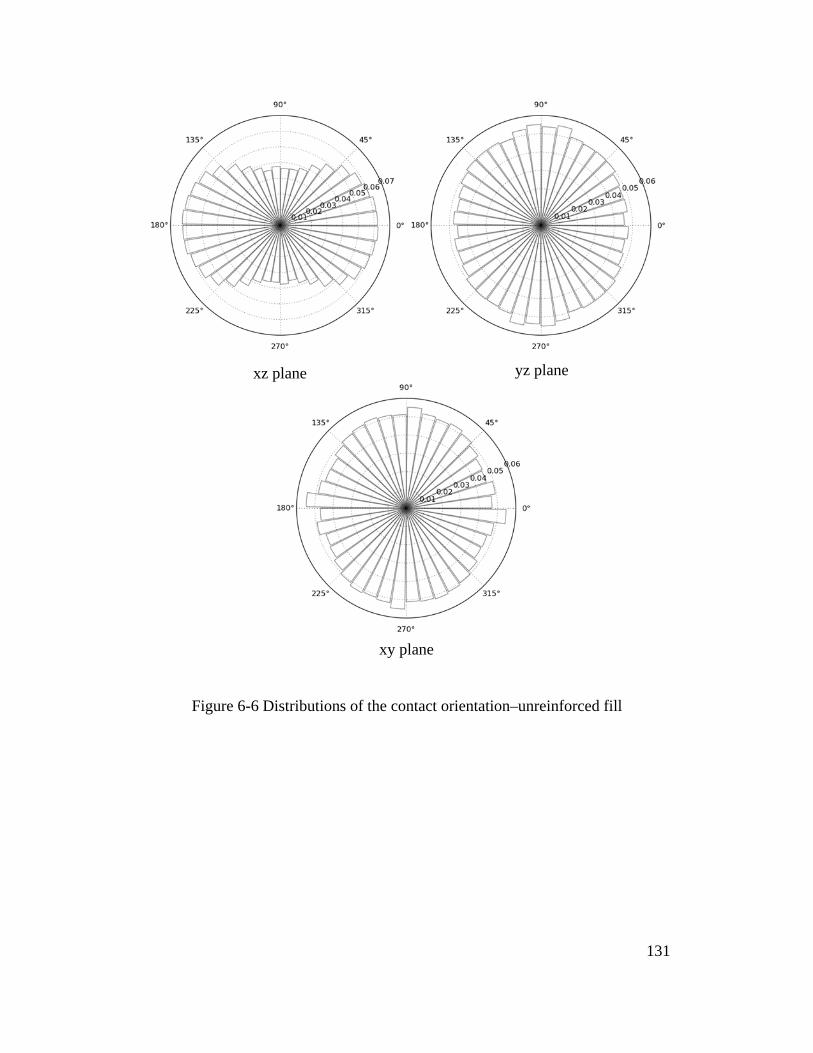
Figure 6-6 Distributions of the contact orientation–unreinforced fill
xz plane yz plane
xy plane
131
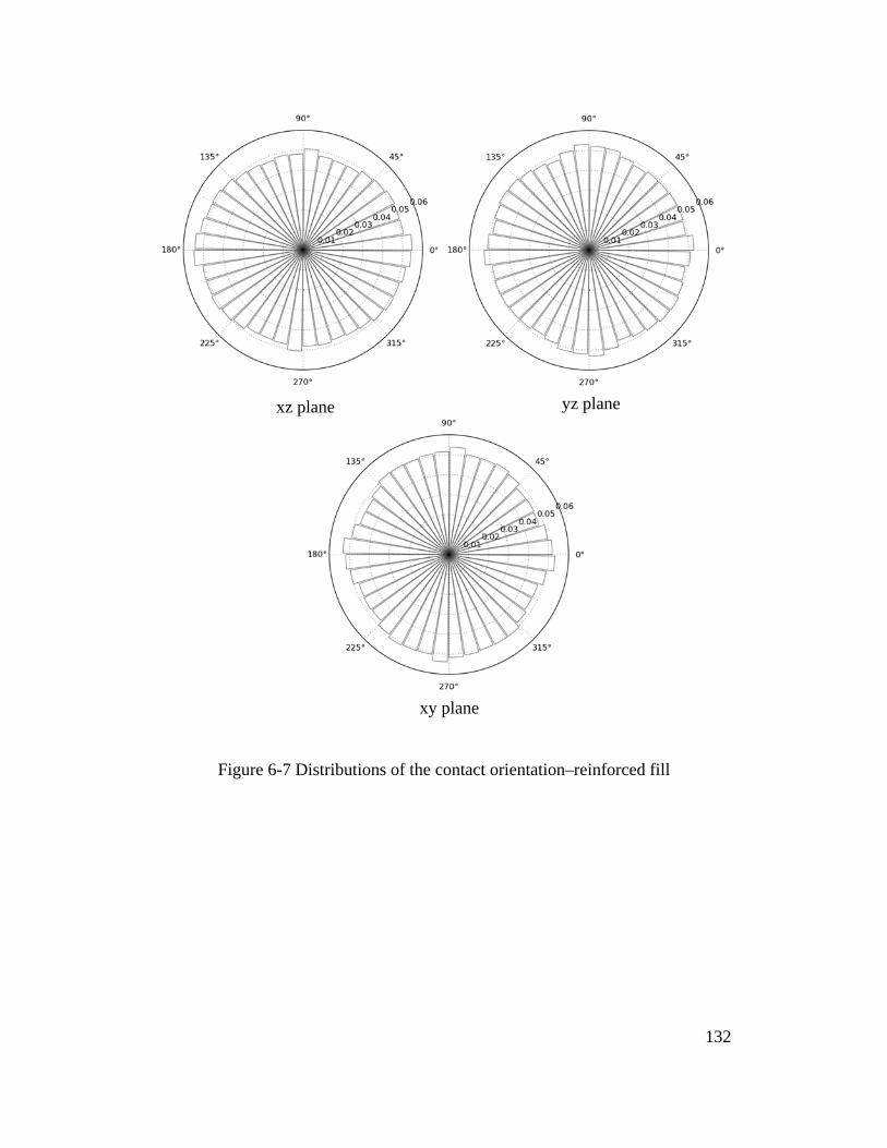
Figure 6-7 Distributions of the contact orientation–reinforced fill
xz plane yz plane
xy plane
132
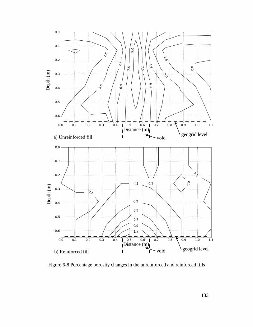
Figure 6-8 Percentage porosity changes in the unreinforced and reinforced fills
Distance (m)
Dep
th (m
)
Distance (m)
Dep
th (m
)
a) Unreinforced fill
b) Reinforced fill
geogrid level void
geogrid level void
133

Figure 6-9 Stress distributions in the unreinforced fill
Distance (m)
Dep
th (m
)
Distance (m)
Dep
th (m
)
a) Vertical stress
b) Horizontal stress
geogrid level void
geogrid level void
134
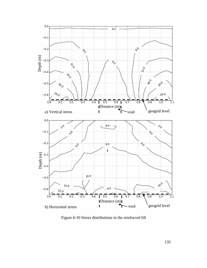
Figure 6-10 Stress distributions in the reinforced fill
Distance (m)
Dep
th (m
)
Distance (m)
Dep
th (m
)
a) Vertical stress
b) Horizontal stress
geogrid level void
geogrid level void
135
6.5. Summary and Conclusions
This study investigated the 3D soil-geogrid interaction using the developed FE-
DE framework. The soil was modeled using DE while the geogrid was modeled
using FE. The interaction between the DE and FE domains was ensured by using
interface elements. The developed framework was used to investigate behavior of
geogrid reinforced fill over void. The 3D geometry of the geogrid, its deformation
and stress distribution were represented. The microscopic behavior of the soil
domain relative to soil displacements, contact orientations, stresses and porosity
changes were analyzed.
The use of geogrid to reinforce a fill over a void is effective in preventing soil
from moving toward the void. The stability of the fill was therefore improved.
The change in porosity in the geogrid reinforced fill was much smaller than for
the unreinforced case. The formation of soil arching produced a stress
redistribution in the fill. A reduction of vertical and horizontal stresses above the
void location was observed. Vertical stresses increased in the vicinity of the void
while the largest horizontal stresses were obtained at top of the fill layer.
The proposed coupled FE-DE method has proven to be effective in capturing soil-
geogrid interaction and analyzing the behavior of both geogrid and surrounding
material.
136
CHAPTER 7
Conclusions and Recommendations
7.1. Conclusions
In this thesis, the discrete element method has been used to analyze the earth
pressure distribution acting on a cylindrical shaft. Numerical results were
compared with experimental and analytical solutions. The efficiency of the
discrete element method in analyzing geotechnical problems involving granular
material and large deformation was demonstrated. Using the validated discrete
element code, a coupled finite-discrete element framework has been developed to
allow soil-structure interaction analysis to be performed. The developed coupled
finite-discrete element method has been implemented and used to analyze selected
soil-structure interaction problems including geogrid pullout test, strip footing
over geogrid-reinforced sand and geogrid-reinforced fill over potential void. The
numerical results of the coupled finite-discrete element simulations were first
validated using experimental data. New insight into the nature of the three-
dimensional interaction between the soil and the reinforcing layer was provided.
The following conclusions can be drawn from the thesis:
1) In chapter 3, a discrete element analysis was performed to investigate the
lateral earth pressure acting on a cylindrical shaft. A modified multi-layer
gravitational packing method was proposed to replicate the real soil
packing procedure. The packing algorithm is capable of representing the
actual particle size distribution. Both the physical and numerical studies
demonstrated that even a limited movement of the shaft wall can lead to a
rapid decrease in the lateral earth pressure acting on the shaft wall. A
movement equivalent to 2.5% to 4% of the shaft radius was required to
reach the full active earth pressure on the wall. Analytical solutions
137
proposed by Terzaghi and Berezantzev provided good agreement with the
observed and calculated pressure distributions. A decrease in radial stresses
and an increase in circumferential stresses in the vicinity of the shaft due to
the arching effect were observed. Results obtained in this phase of the
analysis provided the needed confidence in the discrete element framework
that has been further used in developing the coupled Finite-Discrete
element framework.
2) In chapter 4, a coupled Finite-Discrete element framework was developed
to simulate the soil-structure interaction. This algorithm allows for the
coupling of the finite and discrete element methods. The interaction
between the finite and discrete element domains is assured using interface
elements. A multiple-time-step scheme was applied to optimize the
computational cost. The developed algorithm was used to investigate the
behavior of a biaxial geogrid embedded in granular material and subjected
to pullout loading. The geogrid was modeled using finite elements while
the backfill material was modeled using discrete elements. A good
agreement between numerical results and experimental data was observed.
For the investigated geogrid and soil conditions, largest displacements and
stresses in the geogrid occurred near the front side of the box with rapid
decrease with distance away from the geogrid. The contribution of the
frictional component to the total pullout resistance was found to be larger
than the bearing resistance. It was also found that the contribution of the
bearing resistance to the overall capacity increased as the geogrid
displacement increased. The soil movement and the contact force
distribution within the soil domain agreed well with experimental
observations.
3) In chapter 5, the developed coupled Finite-Discrete element framework
was implemented to analyze a strip footing over geogrid-reinforced sand.
Both unreinforced and geogrid reinforced foundations were studied from
which the efficiency of geogrid reinforcement was investigated. Validation
138
of the developed method was performed by simulating a laboratory
experiment and comparing the calculated and measured data. An increase
in the ultimate bearing capacity of the footing was found to depend on the
number of reinforcing layers. Geogrid deformation and tensile stress for the
case of one geogrid layer were found to be larger than those calculated for
the case of two geogrid layers. The upper geogrid layer experienced larger
deformation and tensile stress compared to the lower layer. At the ultimate
load, a punching shear failure occurred above the geogrid followed by a
general shear failure below the geogrid. An increase in the vertical stresses
in the soil was also observed with the use of geogrid reinforcement.
4) In chapter 6, the behavior of a geogrid-reinforced fill over strong formation
containing void was studied using the developed Finite-Discrete element
method. The efficiency of the geogrid in protecting the overlying fill layer
was investigated. The three-dimensional interaction between the soil and
the geogrid was also analyzed. The use of geogrid to reinforce a fill layer
over a locally developed void is effective in preventing soil from excessive
movement and improving the stability of the fill layer. The change in
porosity in the geogrid reinforced fill was found to be much smaller
compared to the unreinforced case. The developed soil arching resulted in
stress redistribution in the fill with a reduction of vertical and horizontal
stresses above the void location. Vertical stresses increased in the vicinity
of the void while the largest horizontal stresses were observed at top of the
fill layer.
5) The coupled finite-discrete element analysis has proven its efficiency in
analyzing soil-structure interaction problems. The framework has been
implemented in an open source code with computational engines written in
C++ and scripts written in Python.
139
7.2. Recommendations for future work
Various soil-structure interaction problems can be studied using the developed
coupled finite-discrete element framework including:
• Earth pressure distribution on flexible pipes buried in granular backfill
material.
• Cyclic loading of geogrid-reinforced ballast.
• Pile driving in granular material.
Computational fluid dynamics (CFD) can be coupled with the finite-discrete
element framework to investigate soil-structure interaction problems involving
groundwater. Computational engines for CFD can be written and incorporated
into the existing framework. The coupling can also be performed using an
external CFD package as an add-on such as OpenFOAM and CCFD.
The computational parts of the coupled finite-discrete element framework are
written in C++ with object oriented approach. Scripts are built using Python,
which assures rapid and flexible simulation construction. However, capability of
the graphical interface is still limited. Additional effort to improve the graphical
interface is therefore encouraged. Advanced constitutive models for the finite
elements can also be added to the framework to allow for a wide range of
structural elements to be modeled and enhance the capability of the analysis tool.
140
APPENDIX A
User Manual for the Developed 3D Coupled Finite-Discrete Element Analysis Tool
141
A.1. INTRODUCTION
This appendix presents a user manual for the developed 3D coupled Finite-
Discrete element analysis. The developed framework is implemented in YADE, an
open source code for DE analysis. Since both FE and DE simulations are handled
in a common package, the tool provides an efficient approach for solving coupled
FE-DE geotechnical problems.
The computational parts of the coupled FE-DE framework are written in C++
with object oriented approach. Scripts are built using Python, which assures rapid
and flexible simulation construction. Users who do not wish to modify C++
engines can develop their own analyses using Python scripts. Commands written
in Python are first presented in the User Manual. C++ framework of the analysis
tool is briefly presented in latter section. Many of the commands used in the DE
module are also listed in the YADE’s documentation (https://yade-dem.org/doc/).
Knowledge of Linux operating system, C++ and Python programming languages
is strongly recommended for further development of the coupled FE-DE tool.
142
A.2. INSTALLATION
The developed package can be installed in many Linux distributions. Installations
in Kubuntu and Ubuntu have been verified. It is required to install some external
libraries and packages prior to compiling the package. In Kubuntu, required
libraries and packages can be installed using the following commands:
sudo apt-get install scons cmake libcgal-dev git freeglut3-dev libloki-dev \ libboost-date-time-dev libboost-filesystem-dev libboost-thread-dev \ libboost-program-options-dev libboost-regex-dev fakeroot dpkg-dev \ build-essential g++ libboost-iostreams-dev liblog4cxx10-dev \ python-dev libboost-python-dev ipython python-matplotlib \ libsqlite3-dev python-numpy python-tk gnuplot doxygen \ libgts-dev python-pygraphviz libvtk5-dev python-scientific bzr \ libeigen3-dev binutils-gold python-xlib python-qt4 pyqt4-dev-tools \ gtk2-engines-pixbuf python-argparse libqglviewer-qt4-dev python-imaging \ libjs-jquery python-sphinx python-git python-bibtex libxmu-dev \ libxi-dev libgmp3-dev libcgal-dev help2man libqt3-mt-dev qt3-dev-tools \
After all prerequisites have been installed, the coupled FE-DE codes can be
compiled inside the downloaded directory of the source code:
scons PREFIX=/home/username/directory
For example, we can install the tool inside /home/Thomas/YADE folder:
scons PREFIX=/home/Thomas/YADE
The directory of the installed package can be defined by editing the profile file
scons.profile-default of the source code, for example:
PREFIX=/home/Thomas/YADE
YADE can now be compiled by simply typing:
scons
143
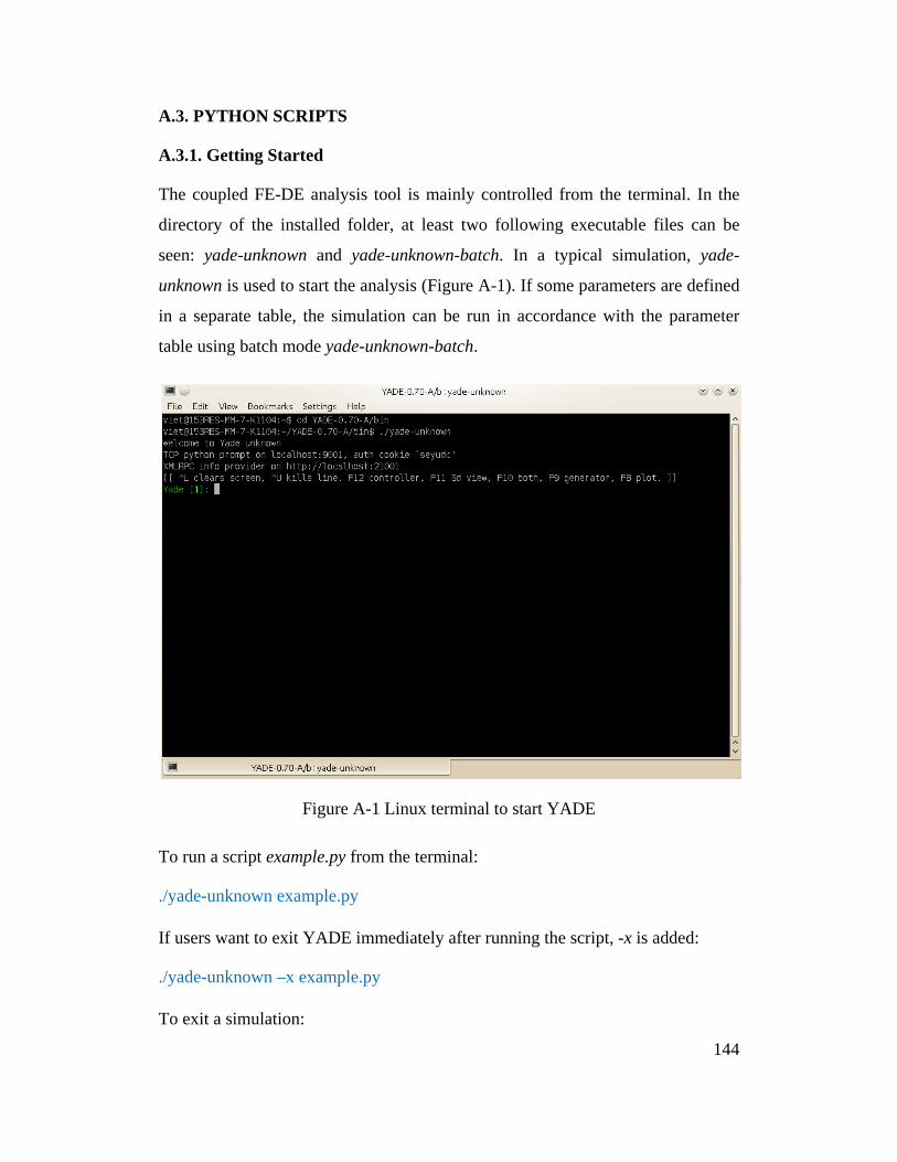
A.3. PYTHON SCRIPTS
A.3.1. Getting Started
The coupled FE-DE analysis tool is mainly controlled from the terminal. In the
directory of the installed folder, at least two following executable files can be
seen: yade-unknown and yade-unknown-batch. In a typical simulation, yade-
unknown is used to start the analysis (Figure A-1). If some parameters are defined
in a separate table, the simulation can be run in accordance with the parameter
table using batch mode yade-unknown-batch.
Figure A-1 Linux terminal to start YADE
To run a script example.py from the terminal:
./yade-unknown example.py
If users want to exit YADE immediately after running the script, -x is added:
./yade-unknown –x example.py
To exit a simulation:
144
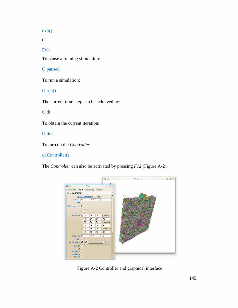
exit()
or
Exit
To pause a running simulation:
O.pause()
To run a simulation:
O.run()
The current time-step can be achieved by:
O.dt
To obtain the current iteration:
O.iter
To turn on the Controller:
qt.Controller()
The Controller can also be activated by pressing F12 (Figure A-2).
Figure A-2 Controller and graphical interface
145

A.3.2. Basic Commands
The number of bodies in a simulation is obtained using:
len(O.bodies)
Time-step for DE simulation can be determined using utils.PWaveTimeStep():
O.dt = 0.5*utils.PWaveTimeStep()
where 0.5 is a user-determined safety coefficient.
The current position of a body can be achieved:
O.bodies[i].state.pos
where O.bodies[i] is ith body stored in the simulation.
For example, positions of all bodies are printed to screen using the following
commands:
# go through all bodies for body in O.bodies: print body.state.pos
Similarly, the current velocity of a body can be determined:
O.bodies[i].state.vel
For example:
for body in O.bodies: print body.state.vel
To get information of the shape of a body:
O.bodies[i].shape
For example, radii of spherical particles with ids from 20 to 23 are printed:
for i in range (20, 24): print O.bodies[i].shape.radius
146
Material of a body is achieved by:
O.bodies[i].mat
For example:
for body in O.bodies:
# check body's Id if body.id < 5:
# print density print body.mat.density
To investigate forces acting on ith element:
O.forces.f(i)
For example:
# go through all bodies for i in range (0, len(O.bodies)):
# print the first component of the force print O.forces.f(i)[1]
The interaction between two particles i and j can be checked using:
O.interactions[i,j]
For example:
# loop through all interactions for I in O.interactions:
# print ids of the two particles in contact print I.id1, I.id2
A.3.3. Sample Generation
The coupled FE-DE framework consists of several types of elements which can
be categorized as:
• DE elements: spheres, clumps, walls, boxes and facets.
147
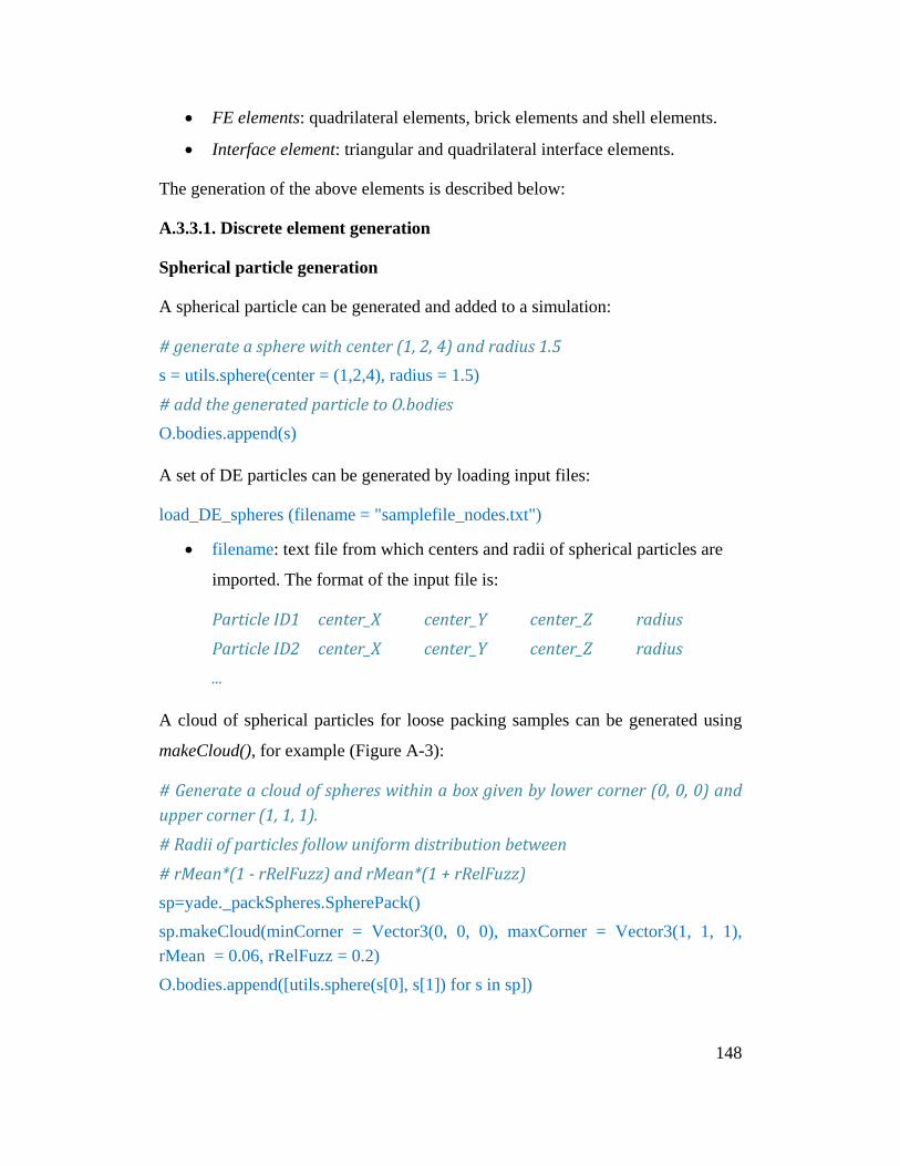
• FE elements: quadrilateral elements, brick elements and shell elements.
• Interface element: triangular and quadrilateral interface elements.
The generation of the above elements is described below:
A.3.3.1. Discrete element generation
Spherical particle generation
A spherical particle can be generated and added to a simulation:
# generate a sphere with center (1, 2, 4) and radius 1.5 s = utils.sphere(center = (1,2,4), radius = 1.5)
# add the generated particle to O.bodies O.bodies.append(s)
A set of DE particles can be generated by loading input files:
load_DE_spheres (filename = "samplefile_nodes.txt")
• filename: text file from which centers and radii of spherical particles are
imported. The format of the input file is:
Particle ID1 center_X center_Y center_Z radius
Particle ID2 center_X center_Y center_Z radius ...
A cloud of spherical particles for loose packing samples can be generated using
makeCloud(), for example (Figure A-3):
# Generate a cloud of spheres within a box given by lower corner (0, 0, 0) and upper corner (1, 1, 1). # Radii of particles follow uniform distribution between
# rMean*(1 - rRelFuzz) and rMean*(1 + rRelFuzz) sp=yade._packSpheres.SpherePack() sp.makeCloud(minCorner = Vector3(0, 0, 0), maxCorner = Vector3(1, 1, 1), rMean = 0.06, rRelFuzz = 0.2) O.bodies.append([utils.sphere(s[0], s[1]) for s in sp])
148
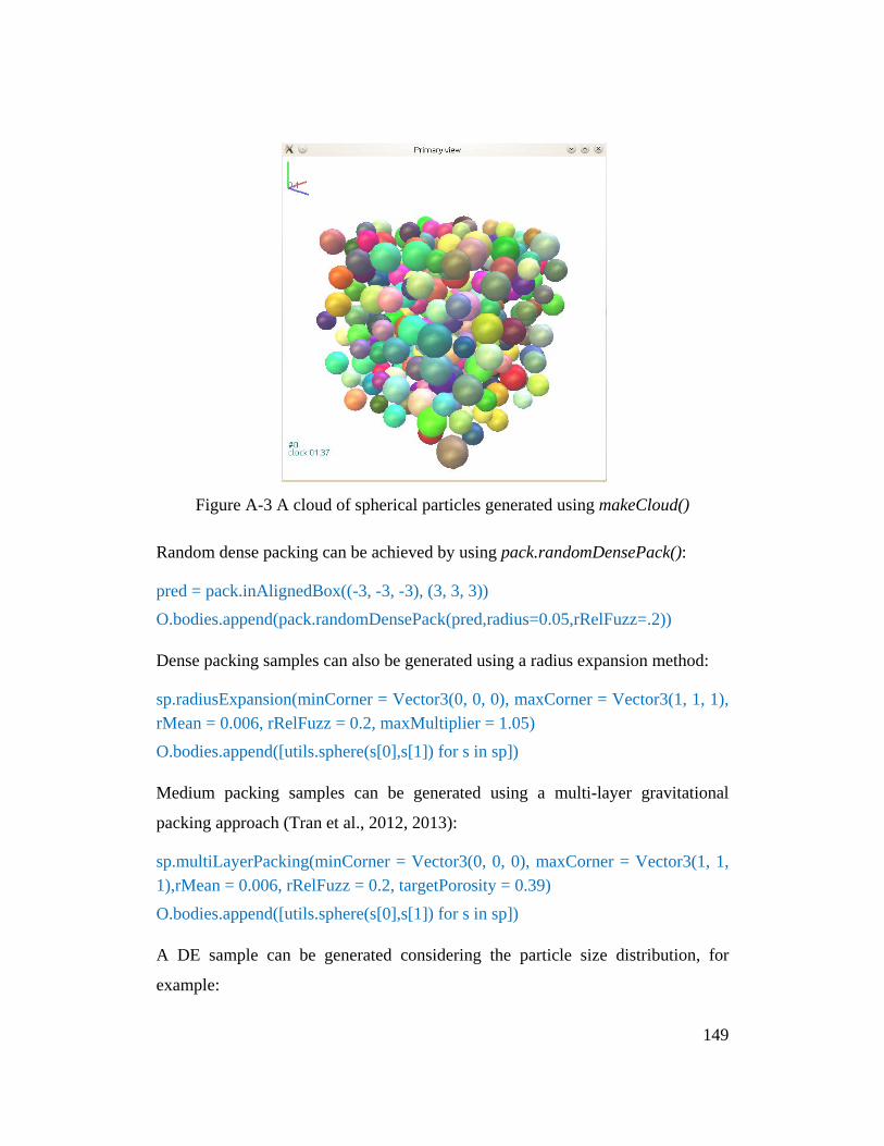
Figure A-3 A cloud of spherical particles generated using makeCloud()
Random dense packing can be achieved by using pack.randomDensePack():
pred = pack.inAlignedBox((-3, -3, -3), (3, 3, 3)) O.bodies.append(pack.randomDensePack(pred,radius=0.05,rRelFuzz=.2))
Dense packing samples can also be generated using a radius expansion method:
sp.radiusExpansion(minCorner = Vector3(0, 0, 0), maxCorner = Vector3(1, 1, 1), rMean = 0.006, rRelFuzz = 0.2, maxMultiplier = 1.05) O.bodies.append([utils.sphere(s[0],s[1]) for s in sp])
Medium packing samples can be generated using a multi-layer gravitational
packing approach (Tran et al., 2012, 2013):
sp.multiLayerPacking(minCorner = Vector3(0, 0, 0), maxCorner = Vector3(1, 1, 1),rMean = 0.006, rRelFuzz = 0.2, targetPorosity = 0.39) O.bodies.append([utils.sphere(s[0],s[1]) for s in sp])
A DE sample can be generated considering the particle size distribution, for
example:
149
sieve = []
# add a sieve with particle size 0.0075 and % (in mass) of finer particles: 0% sieve.append((0.0075,0)) sieve.append((0.01,85)) sieve.append((0.025,97)) sieve.append((0.03,100)) sp. makeCloud (minCorner = Vector3(0, 0, 0), maxCorner = Vector3(1, 1, 1),sieveMass = sieve, targetPorosity = 0.39) O.bodies.append([utils.sphere(s[0],s[1]) for s in sp])
Clump generation
Rigid aggregate of individual particles can be generated using appendClumped(),
for example (Figure A-4):
s1 = utils.sphere(center = (0, 1, 0), radius = 0.5) s2 = utils.sphere(center = (0, 1.6, 0), radius = 0.6)
#Tie two spheres together and add the generated clump to O.bodies O.bodies. appendClumped ([s1, s2])
Wall generation
A rigid wall can be generated using utils.box() such as:
O.bodies.append(utils.box(center=[-1, 0, 1],extents=[1, 1, 0]))
• center: center point of the box.
• extents: half lengths of the box sides.
Box generation
In order to generate a box, a function aabbWalls() can be used, for example:
mn, mx=Vector3(0,0,0),Vector3(1,1,1) walls=utils.aabbWalls([mn,mx],thickness=0.05) O.bodies.append(walls)
Facet generation
Facets are generated using utils.facet() such as:
150
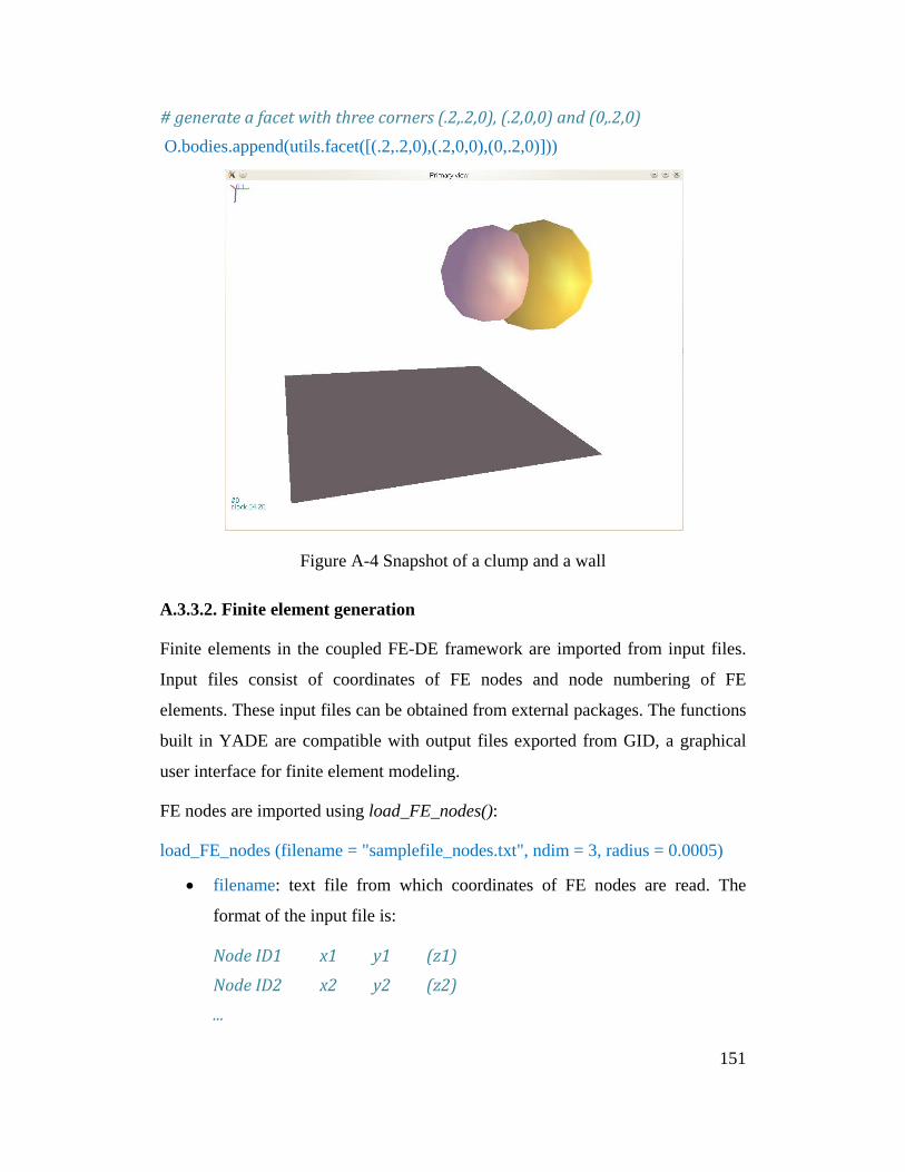
# generate a facet with three corners (.2,.2,0), (.2,0,0) and (0,.2,0) O.bodies.append(utils.facet([(.2,.2,0),(.2,0,0),(0,.2,0)]))
Figure A-4 Snapshot of a clump and a wall
A.3.3.2. Finite element generation
Finite elements in the coupled FE-DE framework are imported from input files.
Input files consist of coordinates of FE nodes and node numbering of FE
elements. These input files can be obtained from external packages. The functions
built in YADE are compatible with output files exported from GID, a graphical
user interface for finite element modeling.
FE nodes are imported using load_FE_nodes():
load_FE_nodes (filename = "samplefile_nodes.txt", ndim = 3, radius = 0.0005)
• filename: text file from which coordinates of FE nodes are read. The
format of the input file is:
Node ID1 x1 y1 (z1)
Node ID2 x2 y2 (z2) ...
151
• ndim: number of dimensions of the simulated problem.
• radius: radius of FE nodes, for illustration purpose only.
Solid FE elements are imported using load_solid_elements():
load_solid_elements (filename = "samplefile_elements.txt", ndim = 3, elementType = "Hexahedron8N8I", matFlag = "elastic")
• filename: text file from which FE elements are imported. The format of
the file is:
Element ID1 Node ID1 Node ID2 Node ID3 ... Element ID2 Node ID1 Node ID2 Node ID3 ...
...
• ndim: number of dimensions of the simulated problem.
• elementType: type of FE elements. Different FE elements are available in
the package including:
"Quadrilateral": quadratic quadrilateral element with eight integration
points.
"Hexahedron8N1I": eight-node quadratic brick element with one
integration point.
"Hexahedron8N8I": eight-node quadratic brick element with eight
integration points.
"Hexahedron20N8I": twenty-node quadratic brick element with eight
integration points.
• matFlag: flag indicating material of FE elements.
"elastic": elastic material
"mohrCoulomb": Mohr-Coulomb failure criterion
Shell elements are imported using load_shell_elements():
load_shell_elements (filename = "samplefile_shells.txt", thickness = 0.002, matFlag = "elastic")
152
• filename: text file from which FE elements are imported. The format of
the text file is:
Element ID1 Node ID1 Node ID2 Node ID3 Node ID4
Element ID2 Node ID1 Node ID2 Node ID3 Node ID4 ...
• thickness: thickness of shell elements
A.3.3.3. Interface element generation
Interface elements are used to assure the interaction between FE and DE domains.
In the coupled FE-DE framework, both triangular facets and quadrilateral facets
are available. A quadrilateral facet is directly defined by the four nodes of the
element (quadrilateral or hexahedron shape) located on the interface. If triangular
facets are used for quadrilateral and hexahedral elements, the contact interface is
divided into four triangular facets by creating a temporary center node. In the case
of triangular or tetrahedron elements, a triangular facet is defined by the three
nodes of the element located on the interface.
Interface elements are imported using load_interface_elements():
load_interface_elements (filename = "samplefile_interfaces.txt", elementType = "Tri-interface")
• filename: text file from which interface elements are imported. The format
of the file is:
Element ID1 Node ID1 Node ID2 Node ID3 (Node ID4) Element ID2 Node ID1 Node ID2 Node ID3 (Node ID4) ...
• elementType: type of interface elements consisting of:
"Tri-interface": triangular interface
"Quad- interface": quadrilateral interface
153
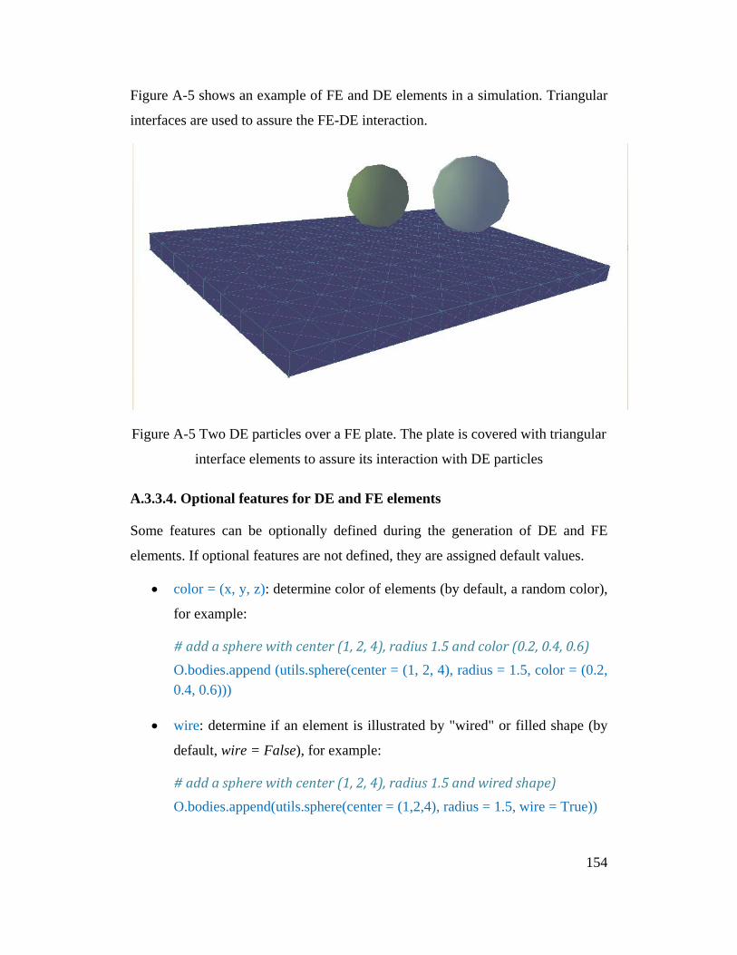
Figure A-5 shows an example of FE and DE elements in a simulation. Triangular
interfaces are used to assure the FE-DE interaction.
Figure A-5 Two DE particles over a FE plate. The plate is covered with triangular
interface elements to assure its interaction with DE particles
A.3.3.4. Optional features for DE and FE elements
Some features can be optionally defined during the generation of DE and FE
elements. If optional features are not defined, they are assigned default values.
• color = (x, y, z): determine color of elements (by default, a random color),
for example:
# add a sphere with center (1, 2, 4), radius 1.5 and color (0.2, 0.4, 0.6) O.bodies.append (utils.sphere(center = (1, 2, 4), radius = 1.5, color = (0.2, 0.4, 0.6)))
• wire: determine if an element is illustrated by "wired" or filled shape (by
default, wire = False), for example:
# add a sphere with center (1, 2, 4), radius 1.5 and wired shape) O.bodies.append(utils.sphere(center = (1,2,4), radius = 1.5, wire = True))
154
• dynamic: determine whether a body will be moved by Newton’s law (by
default, dynamic = True for DE particles and dynamic = False for FE
particles). For example:
# add to O.bodies a non-dynamic sphere O.bodies.append (utils.sphere(center = (1,2,4), radius = 1.5, dynamic = False))
A.3.4. Boundary Conditions
A.3.4.1. Discrete elements
The motion of DE elements can be restrained in several ways:
• dynamic: force a DE element to be non-dynamic (not moved by
NewtonIntegrator) by setting dynamic = False:
utils.sphere([x, y, z), radius, dynamic = False )
• fixed: positions of elements will not change in space by setting fixed =
True, for example:
O.bodies.append(utils.box(center=[0, 0, 0],extents=[.5,.5,.5],fixed=True)).
Note: when fixed = True, DE elements can still be moved manually using
commands in Python or C++.
• blockedDOFs: block any of six degrees of freedom of a particle. For
example, a sphere that can only move in the yz plane is generated:
O.bodies.append(utils.sphere( [1, 2, 4], 1.5)) O.bodies[0].state.blockedDOFs = [‘x’, ‘ry’, ‘rz’]
Restrained conditions of DE particles during simulation can also be achieved
using engines such as UniaxialStrainer(), TriaxialStressController(),
PeriTriaxController(), ForceEngine(), RotationEngine() and TranslationEngine().
A.3.4.2. Finite elements
Movement restraints of FE nodes are assigned using load_restraints():
155
load_restraint(filename = "samplefile_restraints.txt")
The format of the input file is:
Node ID1 Restraint_x1 Restraint_y1 Restraint_z1 Node ID2 Restraint_x2 Restraint_y2 Restraint_z2
...
All restraint values of a FE node are set to zero as default. If a FE node is
restrained in a direction, the restraint value corresponding to that direction is set to
a value of 1.
A.3.5. Assigning Forces and Displacments
A.3.5.1. Discrete elements
Forces acting on DE particles are stored temporarily during one simulation step
and reset to zero at the beginning of the next step. Forces on DE particles can be
added in a simulation step:
# add a force (1, 5, 7) to O.bodies[25] O.forces.addF(25, Vector3(1,5,7))
It is noted that modification of forces using Python is rarely used. It is usually
done using C++.
Forcing the wall to move with a certain velocity can be achieved using:
# translational motion O.bodies[i].state.vel = (0, 0.5, 0)
# rotational motion O.bodies[i].state.angVel=(0.1, 0, 0)
A.3.5.2. Finite elements
External forces acting on a FE domain are imported from input files using
load_external_force():
load_external_force(filename = "samplefile_loads.txt", stepLoad = stepLoading)
156
• stepLoad: a user-defined vector which defines simulation load-steps, for
instance:
stepLoad = [0, 100, 200, 300]
• filename: input file which contains external forces acting on FE nodes.
The format of the input file is:
Node ID1 fx fy fz Node ID2 fx fy fz ...
It is noted that for a certain stepLoad[i], real forces acting on a FE node:
(fx. stepLoad[i], fy. stepLoad[i], fz. stepLoad[i])
For displacement-controlled problems, prescribed displacements can be applied to
certain FE nodes using command:
set_displacements (filename = "samplefile_displacement.txt", stepDisp=stepdisp)
• stepDisp: represents simulation displacement-steps, for instance:
stepDisp = [0, 0.05, 0.1, 0.2]
• filename: the format of the input file is:
Node ID1 Ux Uy Uz
Node ID2 Ux Uy Uz ...
Pre-determined displacements of a FE node for a certain displacement-step are:
(fx. stepDisp[i], fy. stepDisp[i], fz. stepDisp[i]).
A.3.6. Material Models
A.3.6.1. Discrete elements
There are many material models available in YADE, some of them are:
• FrictMat
• CohFrictMat
157
• NormalInelasticMat
• ViscElMat
• CpmMat
• WireMat
New materials are added to the simulation using append command, for example:
O.materials.append(FrictMat(young=4E7,poisson=0.2,frictionAngle=0.5, density=2650, label = "sand"))
A DE particle can be assigned its material properties during generation stage:
O.bodies.append (utils.sphere(center = (1,2,4), radius = 1.5, material ="sand")) load_DE_spheres (filename = "samplefile_nodes.txt", material ="soil")
A.3.6.2. Finite elements
Material properties of FE elements are defined:
For elastic model:
FE_Elastic(young = 3E9, gamma = 15, v = 0.3, EleID = [])
For Mohr_Coulomb model (perfect-plasticity):
FE_MohrCoulomb(young = 3E9, gamma = 15, v = 0.3, c = 2, phi = 0.6, psi = 0, EleID = [])
• young: Young’s modulus
• gamma: specific weight
• v: Poisson’s ratio
• c: cohesion
• phi: friction angle
• psi: dilatancy angle
• EleID: Only FE elements with certain IDs are assigned material
properties. By default, EleID is an empty list and all FE elements are
assigned the newest material properties.
158
A.3.6.3. Interface elements
Material models for DE particles can be used for interface elements. Material
properties of interface elements are defined during their generation:
# add a FrictMat material O.materials.append(FrictMat(young=4E7,poisson=0.2,frictionAngle=0.5,density=2650, label = "interface"))
# Generate interfaces from input file and assign materials. load_interface_elements (filename = "samplefile_interfaces.txt", elementType = "Tri-interface", material ="interface")
A.3.7. Simulation Engines
Main engines of the coupled FE-DE analysis tool can be categorized as follows:
• DE simulation engines
• FE simulation engines
• Interface – DE particle interaction engines
• Additional engines
Different engines types are discussed below:
A.3.7.1. DE simulation engines
A typical DE simulation loop consists of the following tasks (as shown in Figure
A-6):
• Reset forces acting on bodies.
• Approximate and real interaction detections
• Determine physical properties of interactions.
• Calculate forces acting on DE elements from constitutive laws
• Update total forces acting on DE elements
• Update DE element positions
159
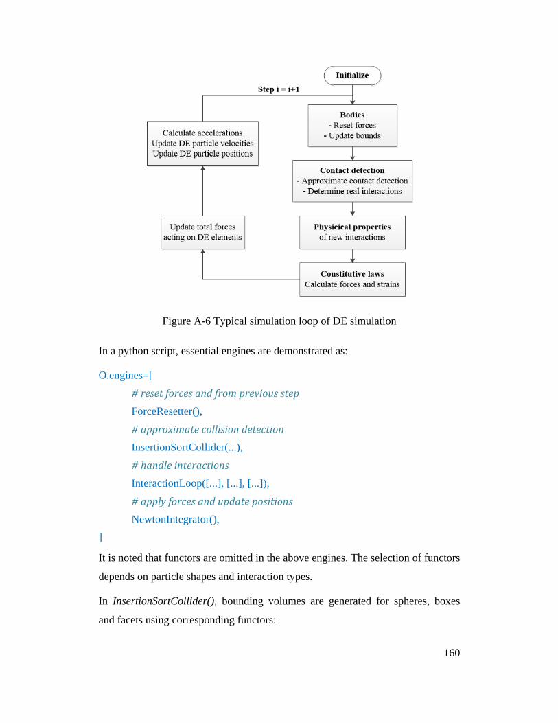
Figure A-6 Typical simulation loop of DE simulation
In a python script, essential engines are demonstrated as:
O.engines=[
# reset forces and from previous step ForceResetter(),
# approximate collision detection InsertionSortCollider(...),
# handle interactions InteractionLoop([...], [...], [...]),
# apply forces and update positions NewtonIntegrator(), ]
It is noted that functors are omitted in the above engines. The selection of functors
depends on particle shapes and interaction types.
In InsertionSortCollider(), bounding volumes are generated for spheres, boxes
and facets using corresponding functors:
160
• Bo1_Sphere_Aabb(): for spheres.
• Bo1_Box_Aabb(): for walls.
• Bo1_Facet_Aabb(): for facets.
In consistency with particle shapes and constitutive laws, interaction functions
determined in InteractionLoop() consist of:
• Functors that determine potential interactions and generate geometrical
information about each potential interaction. Some typical functors are
listed below:
# 6 Dofs sphere-sphere interaction Ig2_Sphere_Sphere_ScGeom6D()
# 6 Dofs wall-sphere interaction Ig2_Box_Sphere_ScGeom6D()
# 6 Dofs facet-sphere interaction Ig2_Facet_Sphere_ScGeom6D()
and:
# 6 Dofs sphere-sphere interaction Ig2_Sphere_Sphere_L6Geom()
# 3 Dofs wall-sphere interaction Ig2_Wall_Sphere_L3Geom()
# 3 Dofs facet-sphere interaction Ig2_ Facet _Sphere_L3Geom()
• Functors that determine non-geometrical features of interactions, some are
listed below:
Ip2_FrictMat_FrictMat_MindlinPhys() Ip2_FrictMat_FrictMat_FrictPhys() Ip2_2xNormalInelasticMat_NormalInelasticityPhys() Ip2_FrictMat_CpmMat_FrictPhys() Ip2_ViscElMat_ViscElMat_ViscElPhys()
161
• Functors that determine constitutive laws, for example:
Law2_ScGeom_MindlinPhys_Mindlin() Law2_ScGeom_FrictPhys_CundallStrack() Law2_ScGeom6D_NormalInelasticityPhys_NormalInelasticity() Law2_ScGeom_CpmPhys_Cpm() Law2_ScGeom_ViscElPhys_Basic()
NewtonIntegrator() is used to apply forces and update positions of DE particles.
This engine also defines gravity acting on DE particles and damping ratio, for
example:
# Apply NewtonIntegrator() with gravity (0, 0, -9.81) and damping ratio of 0.2 NewtonIntegrator (gravity = (0,0,-9.81), damping = 0.2)
Problem 1: A simple script for DE simulation is presented. In the problem, a
sphere and a solid box are generated. The box is fixed while the sphere can move
under gravity. The simulation is set to run 20000 steps.
print "------------Simulation started------------"
# Omega is the super-class that controls the whole simulation O=Omega()
# add a material FrictMat O.materials.append(FrictMat(young=4E7,poisson=0.2,frictionAngle=0.5,density=2650))
# add a fixed box O.bodies.append(utils.box(center=[0,0,0],extents=[.5,.5,.5],color=[0,0,1],fixed = True))
# add a sphere O.bodies.append(utils.sphere([0,0,2],1,color=[0,1,0]))
# Engines which are called consecutively in a calculation step O.engines=[ ForceResetter(), InsertionSortCollider([ Bo1_Sphere_Aabb(),
162
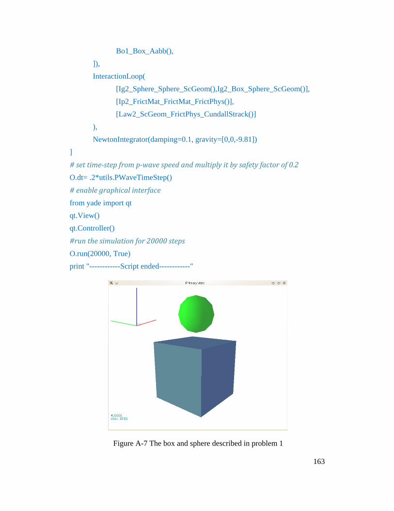
Bo1_Box_Aabb(), ]), InteractionLoop( [Ig2_Sphere_Sphere_ScGeom(),Ig2_Box_Sphere_ScGeom()], [Ip2_FrictMat_FrictMat_FrictPhys()], [Law2_ScGeom_FrictPhys_CundallStrack()] ), NewtonIntegrator(damping=0.1, gravity=[0,0,-9.81]) ]
# set time-step from p-wave speed and multiply it by safety factor of 0.2 O.dt= .2*utils.PWaveTimeStep()
# enable graphical interface from yade import qt qt.View() qt.Controller()
#run the simulation for 20000 steps O.run(20000, True) print "------------Script ended------------"
Figure A-7 The box and sphere described in problem 1
163
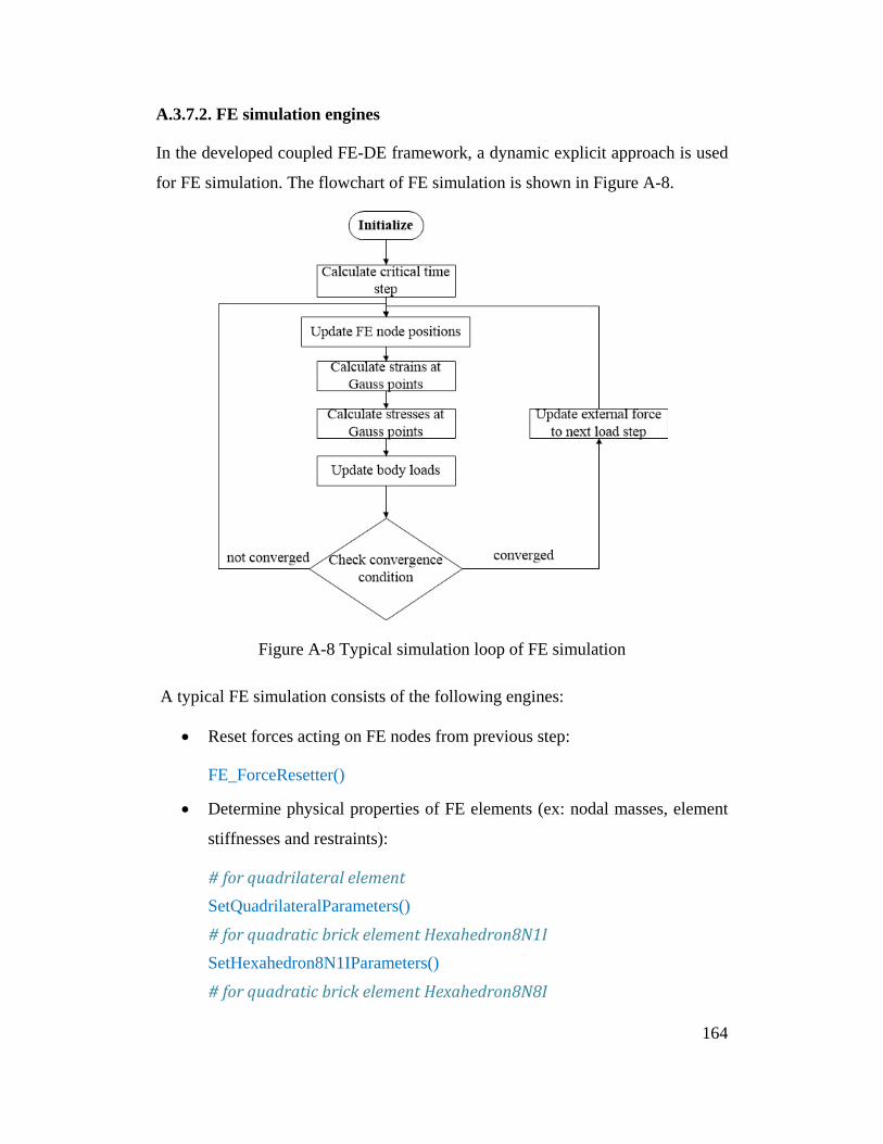
A.3.7.2. FE simulation engines
In the developed coupled FE-DE framework, a dynamic explicit approach is used
for FE simulation. The flowchart of FE simulation is shown in Figure A-8.
Figure A-8 Typical simulation loop of FE simulation
A typical FE simulation consists of the following engines:
• Reset forces acting on FE nodes from previous step:
FE_ForceResetter()
• Determine physical properties of FE elements (ex: nodal masses, element
stiffnesses and restraints):
# for quadrilateral element SetQuadrilateralParameters()
# for quadratic brick element Hexahedron8N1I SetHexahedron8N1IParameters()
# for quadratic brick element Hexahedron8N8I
164
SetHexahedron8N8IParameters()
# for quadratic brick element Hexahedron20N8I SetHexahedron20N8IParameters()
# for shell element SetShellBT4()
• Update geometrical properties of FE elements:
# for quadrilateral element SetGeoQuadrilateral2D()
# for quadratic brick element Hexahedron8N1I and Hexahedron8N8I SetGeoHexahedron()
# for quadratic brick element Hexahedron20N8I SetGeoHexahedron20N()
# for shell element SetGeoShellBT4()
• Determine external loads acting on FE nodes:
SetMultiStepExternalForce()
• Determine FE critical time-step and multiply it by a safety factor:
GlobalTangentStiffnessTimeStepper(ratio = 0.5)
• Set FE time-step equal to n times (n >= 1) DE time-step (for coupled FE-
DE problems):
setdtFEM(n = 100)
• Determine damping coefficient:
DampingRayleigh()
• Check convergence conditions:
CheckConvergence()
• Calculate strains and stresses at Gauss points and update body loads:
# for quadrilateral and brick elements TangentStiffnessCPPM()
165
# for shell element ElasticShellSolver()
• Calculate nodal velocities and update nodal positions
CentralDifference()
• Record outputs
OutputRecording()
Problem 2: This example presents a simple script for FE simulation in which a
square footing over granular soil is simulated. FE elements, material properties,
boundary conditions and loading information are imported from corresponding
input files. Pressure acting on the footing is increased to investigate the
foundation bearing capacity (Figure A-9).
print "------------Simulation started------------" from yade import plot from yade.pack import * O=Omega()
## loading necessary files and generate FEM nodes, elements, loading conditions,..
# Generate FE nodes load_FE_nodes (filename = "squarefooting_nodes.txt", ndim = 3, radius = 0.001)
# Generate FE elements load_solid_elements (filename = "squarefooting_elements.txt", ndim = 3, elementType = "Hexahedron8N8I", matFlag = "elastic")
# Apply boundary conditions load_restraint(filename = "squarefooting_restraints.txt")
# Apply material properties FE_Elastic(young = 3E9, gamma = 15, v = 0.3)
# Apply loading steps step = [0, 100, 200, 300] load_external_force(filename = "squarefooting_loads.txt", stepLoad = step)
## Engines that run during the simulation
166
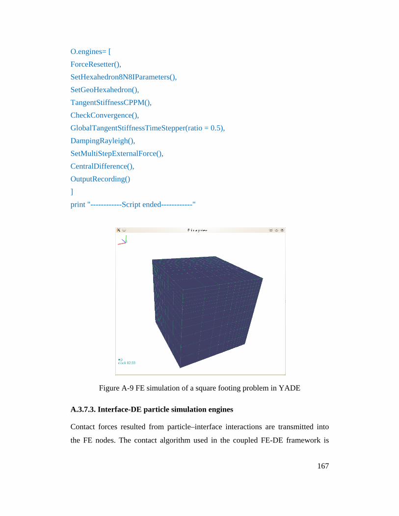
O.engines= [ ForceResetter(), SetHexahedron8N8IParameters(), SetGeoHexahedron(), TangentStiffnessCPPM(), CheckConvergence(), GlobalTangentStiffnessTimeStepper(ratio = 0.5), DampingRayleigh(), SetMultiStepExternalForce(), CentralDifference(), OutputRecording() ] print "------------Script ended------------"
Figure A-9 FE simulation of a square footing problem in YADE
A.3.7.3. Interface-DE particle simulation engines
Contact forces resulted from particle–interface interactions are transmitted into
the FE nodes. The contact algorithm used in the coupled FE-DE framework is
167
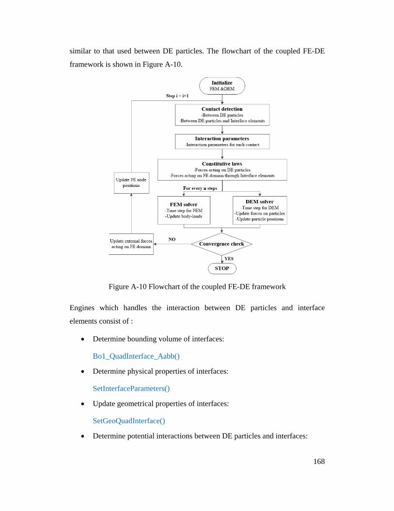
similar to that used between DE particles. The flowchart of the coupled FE-DE
framework is shown in Figure A-10.
Figure A-10 Flowchart of the coupled FE-DE framework
Engines which handles the interaction between DE particles and interface
elements consist of :
• Determine bounding volume of interfaces:
Bo1_QuadInterface_Aabb()
• Determine physical properties of interfaces:
SetInterfaceParameters()
• Update geometrical properties of interfaces:
SetGeoQuadInterface()
• Determine potential interactions between DE particles and interfaces:
168
# 6 Dofs interface-sphere interaction Ig2_ Interface _Sphere_ScGeom6D()
Problem 3: A coupled FE-DE problem which illustrates the interaction between
the two domains is presented. Two spheres are generated using DEM while a
plate is generated using FEM. The two spheres are then allowed to fall onto the
plate. The interaction between the DE particles and the FE plate is modeled using
interface elements (Figure A-11).
print "------------Simulation started------------" from yade import plot from yade.pack import * O=Omega()
## Define materials # for DE particles O.materials.append(FrictMat(young = 10E7, poisson = 0.25, frictionAngle = 0.75, density = 2650, label="sphere"))
#for interfaces O.materials.append(FrictMat(young=10E7, poisson = 0.25, frictionAngle = 0.75, density = 2650, label="interface"))
## Load necessary files and generate FEM nodes, elements, loading conditions,.. # Generate FE nodes load_FE_nodes (filename = "plate_nodes.txt", radius = 0.001)
# Generate FE elements load_solid_elements (filename = "plate_elements.txt", elementType = "Hexahedron8N8I", matFlag = "elastic")
# Generate interface elements load_interface_elements (filename = "plate_interfaces.txt", elementType = "Tri-interface", material ="interface")
# Apply boundary conditions load_restraint(filename = "plate_restraints.txt")
# Apply material properties for FE elements FE_Elastic(young = 3E6, gamma = 16.0, v = 0.25)
169
# Generate 2 spherical DE particles O.bodies.append(utils.sphere([0.3, 0.25, 0.1], 0.05, material = "sphere ")) O.bodies.append(utils.sphere([0.4, 0.15, 0.12], 0.06, material ="sphere "))
# Enable graphical interface from yade import qt qt.View() qt.Controller()
## Engines that run during the simulation O.engines= [ ForceResetter(),
ResetInteractingSphere(),
# execute only at the first step SetHexahedron8N8IParameters(),
# execute only at the first step SetInterfaceParameters(), SetGeoHexahedron(), SetGeoQuadInterface(), TangentStiffnessCPPM(), CheckConvergence(), DampingRayleigh(), SetMultiStepExternalForce(),
# set time-step for DE calculation, O.dt= 0.9*utils.PWaveTimeStep() setdtDEM(ratio = 0.9), InsertionSortCollider([ Bo1_Sphere_Aabb(), Bo1_QuadInterface_Aabb() ]), InteractionLoop([
Ig2_Sphere_Sphere_ScGeom6D(), Ig2_Interface_Sphere_ScGeom6D() ],
[Ip2_2xNormalInelasticMat_NormalInelasticityPhys()], [Law2_ScGeom6D_NormalInelasticityPhys_NormalInelasticity()]
170

), NewtonIntegrator(damping=0.1, gravity = [0,0,-9.81]),
# set time-step for FE calculation = 100 times DE time-sep setdtFEM(n = 10), CentralDifference(), OutputRecording() ] print "------------Script ended------------"
Figure A-11 Deformation of a FE plate in interaction with two DE particles using
the coupled FE-DE framework
It is noted that in the above Python script, the FE time-step is 100 times the DE
time-step. Since the time-step FEt∆ required for FE is much larger than that for
DE ( DEt∆ ), it is not efficient to use a common time-step for both FE and DE
models. Thus, different time-steps for each domain are implemented in the
171
coupling framework to improve the computational efficiency. The time-step in the
FE domain is selected as FE DEt n t∆ = ∆ where n is an integer such that [ ]FE
DE
tn
t∆
≤∆
.
This algorithm is implemented by executing the FE solver for every n DE
computations.
A.3.7.4. Additional engines
Additional functions can be added to the simulation to handle other required
tasks. In YADE, users can develop their own functions either in Python or C++.
Functions written in Python are added to the main engine using PyRunner().
Problem 4: A loose sample is generated inside a container using makeCloud(). A
function named vertical_compress() is written in Python to vertically compress
the top wall until the wall movement reaches a target value of 0.18. Vertical
position and pressure acting on the top wall are monitored during the simulation
using a defined function monitor(). The two functions vertical_compress() and
monitor() are executed for every 100 time-steps (Figure A-12).
print "------------Simulation started------------"
# Omega is the super-class that controls the whole simulation O=Omega()
# add a material type FrictMat O.materials.append(FrictMat(young = 1E7, poisson = 0.25, frictionAngle = 0.6, density = 2650))
# Corners of the box x_min, y_min, z_min = 0.0, 0.0, 0.0 x_max, y_max, z_max = 0.5, 0.2, 0.3
## Generate a container
# top wall O.bodies.append(utils.box(center = [(x_min + x_max)/2, (y_min + y_max)/2, z_max], extents = [(-x_min + x_max)/2, (-y_min + y_max)/2, 0], fixed = True, wire=True))
# bottom wall
172
O.bodies.append(utils.box(center = [(x_min + x_max)/2, (y_min + y_max)/2, z_min], extents = [(-x_min + x_max)/2, (-y_min + y_max)/2, 0], fixed=True, wire=True))
# left wall O.bodies.append(utils.box(center = [x_min, (y_min + y_max)/2, (z_min + z_max)/2], extents=[0, (-y_min + y_max)/2, (-z_min + z_max)/2], fixed=True, wire=True))
# right wall O.bodies.append(utils.box(center = [x_max, (y_min + y_max)/2, (z_min + z_max)/2], extents=[0, (-y_min + y_max)/2, (-z_min + z_max)/2], fixed=True, wire=True))
# front wall O.bodies.append(utils.box(center = [(x_min + x_max)/2, y_min, (z_min + z_max)/2], extents = [(-x_min + x_max)/2, 0, (-z_min + z_max)/2], fixed=True, wire=True))
# behind wall O.bodies.append(utils.box(center = [(x_min + x_max)/2, y_max, (z_min + z_max)/2], extents = [(-x_min + x_max)/2, 0, (-z_min + z_max)/2], fixed=True, wire=True))
# Generate a cloud of spheres sp=yade._packSpheres.SpherePack() sp.makeCloud(Vector3(x_min, y_min, z_min), Vector3(x_max, y_max, z_max), 0.006, 0.2) O.bodies.append([utils.sphere(s[0], s[1]) for s in sp])
# determine whether the top wall is still moved moving_box = True
# Engines which are called consecutively in a calculation step O.engines=[ ForceResetter(), InsertionSortCollider([ Bo1_Sphere_Aabb(), Bo1_Box_Aabb(), ]), InteractionLoop(
173
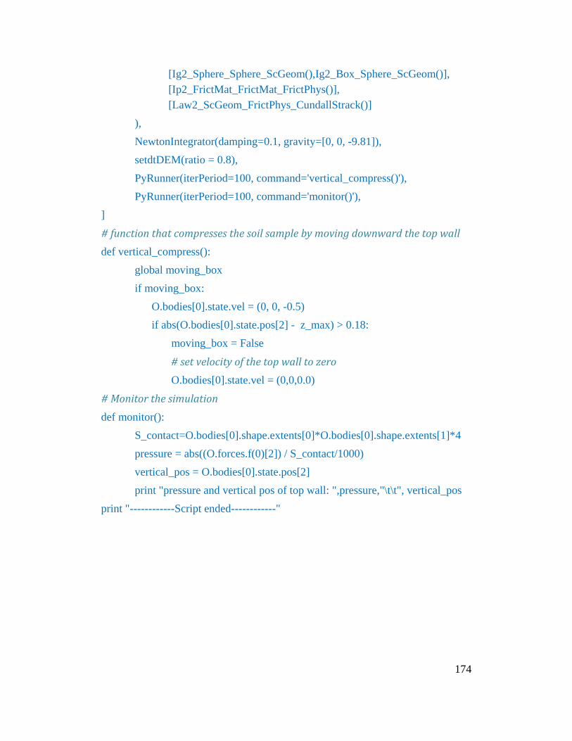
[Ig2_Sphere_Sphere_ScGeom(),Ig2_Box_Sphere_ScGeom()], [Ip2_FrictMat_FrictMat_FrictPhys()], [Law2_ScGeom_FrictPhys_CundallStrack()] ), NewtonIntegrator(damping=0.1, gravity=[0, 0, -9.81]), setdtDEM(ratio = 0.8), PyRunner(iterPeriod=100, command='vertical_compress()'), PyRunner(iterPeriod=100, command='monitor()'), ]
# function that compresses the soil sample by moving downward the top wall def vertical_compress(): global moving_box if moving_box: O.bodies[0].state.vel = (0, 0, -0.5) if abs(O.bodies[0].state.pos[2] - z_max) > 0.18: moving_box = False
# set velocity of the top wall to zero O.bodies[0].state.vel = (0,0,0.0)
# Monitor the simulation def monitor():
S_contact=O.bodies[0].shape.extents[0]*O.bodies[0].shape.extents[1]*4 pressure = abs((O.forces.f(0)[2]) / S_contact/1000) vertical_pos = O.bodies[0].state.pos[2] print "pressure and vertical pos of top wall: ",pressure,"\t\t", vertical_pos
print "------------Script ended------------"
174
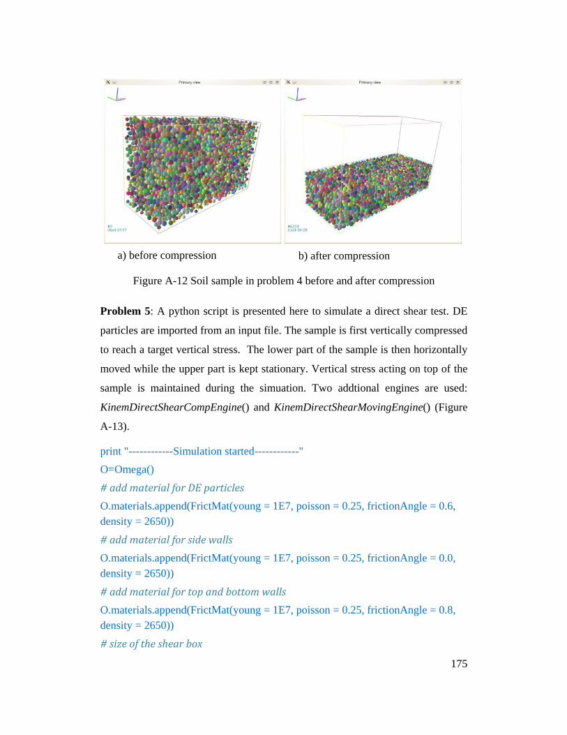
Figure A-12 Soil sample in problem 4 before and after compression
Problem 5: A python script is presented here to simulate a direct shear test. DE
particles are imported from an input file. The sample is first vertically compressed
to reach a target vertical stress. The lower part of the sample is then horizontally
moved while the upper part is kept stationary. Vertical stress acting on top of the
sample is maintained during the simuation. Two addtional engines are used:
KinemDirectShearCompEngine() and KinemDirectShearMovingEngine() (Figure
A-13).
print "------------Simulation started------------" O=Omega()
# add material for DE particles O.materials.append(FrictMat(young = 1E7, poisson = 0.25, frictionAngle = 0.6, density = 2650))
# add material for side walls O.materials.append(FrictMat(young = 1E7, poisson = 0.25, frictionAngle = 0.0, density = 2650))
# add material for top and bottom walls O.materials.append(FrictMat(young = 1E7, poisson = 0.25, frictionAngle = 0.8, density = 2650))
# size of the shear box
a) before compression b) after compression
175
L_x, L_y, L_z = 0.06, 0.0125, 0.06
# names of input and output files sphere_input_file_name = "Direct_shear_test_sphere_input.txt" out_put_file_name = "Direct-shear-test-ouput.txt"
## now define boxes
# lower part, left wall left_low_center, left_low_extents = (0, L_y/2, L_z/2), (0, L_y/2, L_z/2)
# lower part, right wall right_low_center, right_low_extents = (L_x, L_y/2, L_z/2), (0, L_y/2, L_z/2)
# bottom wall bot_center, bot_extents = (L_x/2, 0, L_z/2), (L_x/2, 0, L_z/2)
# lower part, behind wall behind_low_center, behind_low_extents = (L_x/2, L_y/2, 0), (L_x/2, L_y/2, 0)
# lower part, front wall front_low_center, front_low_extents = (L_x/2, L_y/2, L_z), (L_x/2, L_y/2, 0)
# upper part, left wall left_upper_center, left_upper_extents = (0, 3*L_y/2 , L_z/2), (0, L_y/2, L_z/2)
# upper part, right wall right_upper_center, right_upper_extents = (L_x, 3*L_y/2, L_z/2), (0,L_y/2, L_z/2)
# top wall top_center, top_extents = (L_x/2, 2*L_y, L_z/2), (L_x/2, 0, L_z/2)
# upper part, behind wall behind_upper_center, behind_upper_extents=(L_x/2,3*L_y/2,0),(L_x/2,L_y/2, 0)
# upper part, front wall front_upper_center, front_upper_extents = (L_x/2, 3*L_y/2,L_z), (L_x/2,L_y/2, 0)
## generate two additional panels at the middle height of the sample to avoid particles from falling out during shearing, the two panels will be expanded following shearing process. # left panel left_panel_center, left_panel_extents = (0, L_y, L_z/2), (0, 0, L_z/2)
176
# right panel right_panel_center, right_panel_extents = (L_x, L_y , L_z/2), (0, 0, L_z/2)
# now add walls to simulation leftBox_low = utils.box(center = left_low_center, extents = left_low_extents, fixed = True, wire = True, material = O.materials[1]) rightBox_low = utils.box(center = right_low_center, extents = right_low_extents, fixed = True, wire = True, material=O.materials[1]) botBox = utils.box(center = bot_center, extents=bot_extents, fixed = True, wire = True, material=O.materials[2]) behindBox_low = utils.box(center = behind_low_center, extents = behind_low_extents, fixed = True, wire = True, material=O.materials[1]) frontBox_low = utils.box(center = front_low_center, extents = front_low_extents , fixed = True, wire = True, material=O.materials[1]) leftBox_upper = utils.box(center = left_upper_center, extents = left_upper_extents, fixed = True, wire = True, material=O.materials[1]) rightBox_upper = utils.box(center = right_upper_center, extents = right_upper_extents , fixed=True, wire = True, material=O.materials[1]) topBox = utils.box(center=top_center, extents = top_extents, fixed = True, wire = True, material=O.materials[2]) behindBox_upper = utils.box( center = behind_upper_center, extents = behind_upper_extents , fixed=True,wire=True,material=O.materials[1]) frontBox_upper = utils.box( center = front_upper_center, extents = front_upper_extents, fixed=True,wire=True,material=O.materials[1]) leftPanel = utils.box( center = left_panel_center, extents = left_panel_extents, fixed=True,wire=True) rightPanel = utils.box( center = right_panel_center, extents = right_panel_extents, fixed=True,wire=True)
# add to O.bodies O.bodies.append([leftBox_low, rightBox_low, botBox, behindBox_low, frontBox_low, leftBox_upper, rightBox_upper, topBox, behindBox_upper, frontBox_upper,leftPanel, rightPanel])
# add spheres infile = open(sphere_input_file_name,"r") lines = infile.readlines()
177
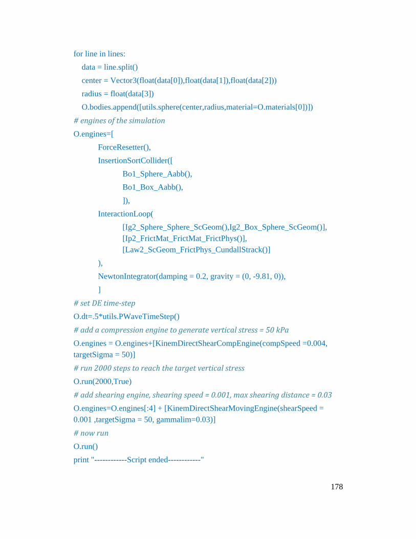
for line in lines: data = line.split() center = Vector3(float(data[0]),float(data[1]),float(data[2])) radius = float(data[3]) O.bodies.append([utils.sphere(center,radius,material=O.materials[0])])
# engines of the simulation O.engines=[ ForceResetter(), InsertionSortCollider([ Bo1_Sphere_Aabb(), Bo1_Box_Aabb(), ]), InteractionLoop( [Ig2_Sphere_Sphere_ScGeom(),Ig2_Box_Sphere_ScGeom()], [Ip2_FrictMat_FrictMat_FrictPhys()], [Law2_ScGeom_FrictPhys_CundallStrack()] ), NewtonIntegrator(damping = 0.2, gravity = (0, -9.81, 0)), ]
# set DE time-step O.dt=.5*utils.PWaveTimeStep()
# add a compression engine to generate vertical stress = 50 kPa O.engines = O.engines+[KinemDirectShearCompEngine(compSpeed =0.004, targetSigma = 50)]
# run 2000 steps to reach the target vertical stress O.run(2000,True)
# add shearing engine, shearing speed = 0.001, max shearing distance = 0.03 O.engines=O.engines[:4] + [KinemDirectShearMovingEngine(shearSpeed = 0.001 ,targetSigma = 50, gammalim=0.03)]
# now run O.run() print "------------Script ended------------"
178
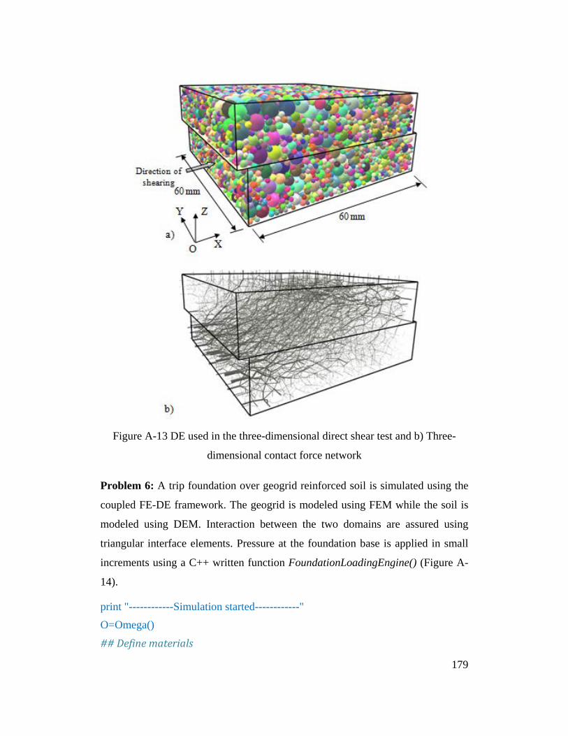
Figure A-13 DE used in the three-dimensional direct shear test and b) Three-
dimensional contact force network
Problem 6: A trip foundation over geogrid reinforced soil is simulated using the
coupled FE-DE framework. The geogrid is modeled using FEM while the soil is
modeled using DEM. Interaction between the two domains are assured using
triangular interface elements. Pressure at the foundation base is applied in small
increments using a C++ written function FoundationLoadingEngine() (Figure A-
14).
print "------------Simulation started------------" O=Omega()
## Define materials
179
# for DE particles O.materials.append (NormalInelasticMat(young=4E7,poisson=0.2, frictionAngle=0.5, density=2650, label="sphere"))
# for interfaces O.materials.append(NormalInelasticMat(young=4E7,poisson=0.2,frictionAngle =0.5, density=2650, label="interface"))
## Load necessary files and generate FEM nodes, elements, loading conditions,.. # Generate FE nodes load_FE_nodes (filename = "foundation_nodes.txt", ndim = 3, radius = 0.001)
# Generate FE elements load_solid_elements (filename = " foundation _elements.txt", ndim = 3, elementType = "Hexahedron8N8I", matFlag = "elastic") load_interface_elements (filename = " foundation _interfaces.txt", elementType = "Tri-interface", material ="interface")
# Apply boundary conditions load_restraint(filename = " foundation _restraints.txt")
# Apply material properties for FE elements FE_Elastic(young = 3E9, gamma = 15, v = 0.3)
# Generate spheres from input file load_DE_spheres(filename = "sphere_nodes.txt", material ="sphere")
# generate the container x_min, y_min, z_min = 0.0, 0.0, 0.0 x_max, y_max, z_max = 1.1, 0.3, 0.6
# add bottom wall O.bodies.append(utils.box(center=[(x_min + x_max)/2, (y_min + y_max)/2, z_min], extents=[(-x_min + x_max)/2, (-y_min + y_max)/2, 0], fixed=True, wire=True))
# add left wall O.bodies.append(utils.box(center=[x_min,(y_min + y_max)/2,(z_min + z_max)/2], extents=[0, (-y_min + y_max)/2,(-z_min + z_max)/2], fixed=True, wire=True))
# add right wall
180
O.bodies.append(utils.box(center=[x_max,(y_min + y_max)/2,(z_min + z_max)/2], extents=[0, (-y_min + y_max)/2,(-z_min + z_max)/2],fixed=True, wire=True))
# add front wall O.bodies.append(utils.box(center=[(x_min + x_max)/2,y_min,(z_min + z_max)/2], extents=[(-x_min + x_max)/2 , 0, (-z_min + z_max)/2 ],fixed=True, wire=True))
# add behind wall O.bodies.append(utils.box(center=[(x_min + x_max)/2,y_max,(z_min + z_max)/2], extents=[(-x_min + x_max)/2 , 0, (-z_min + z_max)/2 ],fixed=True,wire=True))
## generate the strip footing footing_width = 0.1 f_x_min = (x_min + x_max)/2 - footing_width/2 f_x_max = (x_min + x_max)/2 + footing_width/2 f_y_min = y_min f_y_max = y_max f_z_min = z_max
# determine id of the strip footing ID = len(O.bodies)
# add the footing to O.bodies() O.bodies.append(utils.box(center=[(f_x_min + f_x_max)/2,(f_y_min + f_y_max)/2, f_z_min ],extents=[(footing_width)/2, (-f_y_min + f_y_max)/2, 0],fixed=True, wire=False))
# Loading steps: footing pressure increases from 0 to 200 kPa pressure = [] for i in range (0,11): pressure.append(i*20)
# Enable graphical interface from yade import qt qt.View() qt.Controller()
## Engines that run during the simulation
181
O.engines= [ ForceResetter(), FE_ForceResetter(), SetHexahedron8N8IParameters(), SetInterfaceParameters() , SetGeoHexahedron(), SetGeoQuadInterface(), TangentStiffnessCPPM(), CheckConvergence(), DampingRayleigh(), SetMultiStepExternalForce(),
# time-step for DE simulation setdtDEM(ratio = 0.9), InsertionSortCollider([ Bo1_Sphere_Aabb(), Bo1_Box_Aabb(), Bo1_QuadInterface_Aabb() ]), InteractionLoop([ Ig2_Sphere_Sphere_ScGeom6D(), Ig2_Box_Sphere_ScGeom6D(), Ig2_Interface_Sphere_ScGeom6D() ], [Ip2_2xNormalInelasticMat_NormalInelasticityPhys()], [Law2_ScGeom6D_NormalInelasticityPhys_NormalInelasticity()] ), NewtonIntegrator(damping=0.1, gravity=[0, 0, -9.81]),
## Moving the strip foundation downward following defined pressure steps # compression speed = 0.005
182

FoundationLoadingEngine(id_top = ID, val = pressure, compSpeed = 0.005), setdtFEM (n = 100), CentralDifference(), OutputRecording() ] print "------------Script ended------------"
183
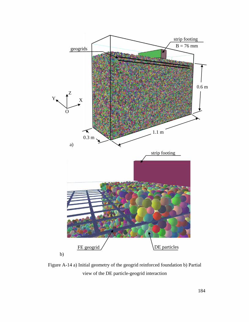
Figure A-14 a) Initial geometry of the geogrid reinforced foundation b) Partial
view of the DE particle-geogrid interaction
strip footing
DE particles FE geogrid b)
1.1 m 0.3 m
0.6 m
strip footing B = 76 mm geogrids
a)
O
Z X Y
184
Problem 7: A geogrid pullout test is simulated using the coupled FE-DE
framework. The geogrid is modeled using FEM while the soil is modeled using
DEM. Vertical stress acting on top of the sample is kept constant during the test
using a stress control mechanism. The pullout procedure is numerically performed
using a displacement control approach in which lateral displacements were
applied in different increments. Two new C++ built engines are used in the
simulation: PressureControlEngine() to control the vertical stress and
GeogridPulloutEngine() to numerically simulate the pullout of the geogrid
(Figure A-15).
print "------------Simulation started------------" O=Omega()
## Define materials # for DE particles O.materials.append(NormalInelasticMat(young=4E7,poisson=0.2,frictionAngle=0.5, density=2650, label="sphere"))
# for interfaces O.materials.append(NormalInelasticMat(young=4E7,poisson=0.2,frictionAngle=0.5, density=2650, label="interface"))
## load necessary files and generate FEM nodes, elements, loading conditions,.. # generate FE nodes load_FE_nodes (filename = "geogrid_nodes.txt", ndim = 3, radius = 0.001)
# generate FE elements load_solid_elements (filename = "geogrid_elements.txt", elementType = "Hexahedron8N8I", matFlag = "elastic")
# generate interfaces load_interface_elements (filename = "geogrid_interfaces.txt", elementType = "Tri-interface", material ="interface")
# apply boundary conditions load_restraint(filename = "geogrid_restraints.txt")
# apply material properties for FE elements FE_Elastic(young = 3E9, gamma = 15, v = 0.3)
# load spheres from input file
185
load_DE_spheres(filename = "sphere_nodes.txt", material ="sphere")
# generate the box x_min, y_min, z_min = 0.0, 0.0, 0.0 x_max, y_max, z_max = 0.68, 0.3, 0.62
# determine id of the top wall ID = len(O.bodies)
## add walls of the container # top wall O.bodies.append(utils.box(center=[(x_min + x_max)/2,(y_min + y_max)/2, z_max], extents=[(-x_min + x_max)/2, (-y_min + y_max)/2, 0],fixed=True, wire=True))
# bottom wall O.bodies.append(utils.box(center=[(x_min + x_max)/2,(y_min + y_max)/2, z_min], extents=[(-x_min + x_max)/2, (-y_min + y_max)/2, 0],fixed=True, wire=True))
# left wall O.bodies.append(utils.box(center=[x_min,(y_min + y_max)/2,(z_min + z_max)/2], extents=[0, (-y_min + y_max)/2,(-z_min + z_max)/2],fixed=True, wire=True))
# right wall O.bodies.append(utils.box(center=[x_max,(y_min + y_max)/2,(z_min + z_max)/2], extents=[0, (-y_min + y_max)/2,(-z_min + z_max)/2],fixed=True, wire=True))
# front wall O.bodies.append(utils.box(center=[(x_min + x_max)/2,y_min,(z_min + z_max)/2], extents=[(-x_min + x_max)/2 , 0, (-z_min + z_max)/2 ],fixed=True, wire=True)) # behind wall O.bodies.append(utils.box(center=[(x_min + x_max)/2,y_max,(z_min + z_max)/2], extents=[(-x_min + x_max)/2 , 0, (-z_min + z_max)/2 ],fixed=True, wire=True))
# pullout displacement: from 0 to 40 mm geogrid_disp = [] for i in range (0,11):
186
geogrid_disp.append(i*0.004)
# target vertical stress acting on top of the sample (kPa) vertical_stress = 50
# enable graphical interface from yade import qt qt.View() qt.Controller()
## Engines that run during simulation O.engines= [ ForceResetter(), ResetInteractingSphere(), SetHexahedron8N8IParameters(), SetInterfaceParameters() , SetGeoHexahedron(), SetGeoQuadInterface(), TangentStiffnessCPPM(), CheckConvergence(), DampingRayleigh(), SetMultiStepExternalForce(), setdtDEM(ratio = 0.9), #set time-step for DE calculation InsertionSortCollider([ Bo1_Sphere_Aabb(), Bo1_Box_Aabb(), Bo1_QuadInterface_Aabb() ]), InteractionLoop([ Ig2_Sphere_Sphere_ScGeom6D(), Ig2_Box_Sphere_ScGeom6D(), Ig2_Interface_Sphere_ScGeom6D() ], [Ip2_2xNormalInelasticMat_NormalInelasticityPhys()], [Law2_ScGeom6D_NormalInelasticityPhys_NormalInelasticity()] ), NewtonIntegrator(damping=0.1,gravity=[0,0,-9.81]),
187
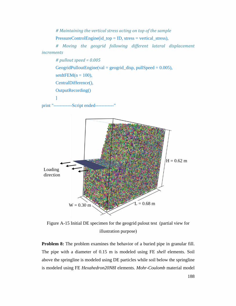
# Maintaining the vertical stress acting on top of the sample PressureControlEngine(id_top = ID, stress = vertical_stress),
# Moving the geogrid following different lateral displacement increments # pullout speed = 0.005 GeogridPulloutEngine(val = geogrid_disp, pullSpeed = 0.005), setdtFEM(n = 100), CentralDifference(), OutputRecording() ] print "------------Script ended------------"
Figure A-15 Initial DE specimen for the geogrid pulout test (partial view for
illustration purpose)
Problem 8: The problem examines the behavior of a buried pipe in granular fill.
The pipe with a diameter of 0.15 m is modeled using FE shell elements. Soil
above the springline is modeled using DE particles while soil below the springline
is modeled using FE Hexahedron20N8I elements. Mohr-Coulomb material model
L = 0.68 m
H = 0.62 m
W = 0.30 m
Loading direction
188
is used for the FE soil domain while elastic behavior is assumed for the pipe. A
material NormalInelasticMat() is used for the DE particles. Vertical stresses are
uniformly applied to top of the fill using PressureControlEngine(). Deformations
and earth pressures acting on the pipe at different vertical stresses are illustrated
in Figure A-16.
print "------------Simulation started------------" O=Omega()
## Define materials # for DE particles O.materials.append(NormalInelasticMat(young=10E7,poisson=0.3,frictionAngle=0.65, density=2650, label="sphere")) # for interfaces O.materials.append(NormalInelasticMat(young=10E7,poisson=0.3,frictionAngle=0.4, density=2650, label="interface"))
## load necessary files and generate FEM nodes, elements, loading conditions,.. # generate FE nodes load_FE_nodes (filename = "fill_nodes.txt", ndim = 3, radius = 0.001)
# generate FE elements for soil domain load_solid_elements (filename = "fill_FE_soil.txt", elementType = "Hexahedron20N8I", matFlag = "mohrCoulomb")
# generate FE shell element for pipe load_shell_elements (filename = "fill_FE_shells.txt", thickness = 0.004, matFlag = "elastic")
# generate interfaces load_interface_elements (filename = "fill_interfaces.txt", elementType = "Tri-interface", material ="interface") # apply boundary conditions load_restraint(filename = "fill_restraints.txt")
# apply material properties for FE soil elements FE_MohrCoulomb(young = 20E6, gamma = 19, v = 0.3, c = 2, phi = 0.6, psi = 0, forShell = False)
# apply material properties for FE shell elements
189
FE_Elastic (young = 450E6, gamma = 15, v = 0.46, forShell = True)
# load spheres from input file load_DE_spheres(filename = "sphere_nodes.txt", material ="sphere")
# generate the box x_min, y_min, z_min = 0.0, 0.0, -0.1 x_max, y_max, z_max = 0.8, 0.15, 0.4
# determine id of the top wall ID = len(O.bodies)
## add walls of the container, the bottom wall is not generated letting soil be in contact with the FE domain.
# top wall O.bodies.append(utils.box(center=[(x_min + x_max)/2,(y_min + y_max)/2, z_max], extents=[(-x_min + x_max)/2, (-y_min + y_max)/2, 0],fixed=True, wire=True))
# left wall O.bodies.append(utils.box(center=[x_min,(y_min + y_max)/2,(z_min + z_max)/2], extents=[0, (-y_min + y_max)/2,(-z_min + z_max)/2],fixed=True, wire=True))
# right wall O.bodies.append(utils.box(center=[x_max,(y_min + y_max)/2,(z_min + z_max)/2], extents=[0, (-y_min + y_max)/2,(-z_min + z_max)/2],fixed=True, wire=True))
# front wall O.bodies.append(utils.box(center=[(x_min + x_max)/2,y_min,(z_min + z_max)/2], extents=[(-x_min + x_max)/2 , 0, (-z_min + z_max)/2 ],fixed=True, wire=True))
# behind wall O.bodies.append(utils.box(center=[(x_min + x_max)/2,y_max,(z_min + z_max)/2], extents=[(-x_min + x_max)/2 , 0, (-z_min + z_max)/2 ],fixed=True, wire=True))
# loading steps: vertical stress increases from 0 to 500 kPa pressure = [] for i in range (0,11): pressure.append(i*50)
190
# enable graphical interface from yade import qt qt.View() qt.Controller()
## Engines that run during simulation O.engines= [ ForceResetter(), ResetInteractingSphere(), SetHexahedron8N8IParameters(),
# physical parameters of shell elements SetShellBT4(), SetInterfaceParameters(), SetGeoHexahedron(),
# geometrical parameters of shell elements SetGeoShellBT4(), SetGeoQuadInterface(),
# stresses, strains, body loads for brick elements TangentStiffnessCPPM(),
# stresses, strains, body loads for shell elements ElasticShellSolver(), CheckConvergence(), DampingRayleigh(), SetMultiStepExternalForce(), setdtDEM(ratio = 0.9), InsertionSortCollider([ Bo1_Sphere_Aabb(), Bo1_Box_Aabb(), Bo1_QuadInterface_Aabb() ]), InteractionLoop([ Ig2_Sphere_Sphere_ScGeom6D(), Ig2_Box_Sphere_ScGeom6D(),
191

Ig2_Interface_Sphere_ScGeom6D() ], [Ip2_2xNormalInelasticMat_NormalInelasticityPhys()], [Law2_ScGeom6D_NormalInelasticityPhys_NormalInelasticity()] ), NewtonIntegrator(damping=0.1,gravity=[0, 0, -9.81]),
# maintaining the vertical stress acting on top of the sample PressureControlEngine(id_top = ID, stress = pressure), setdtFEM(n = 100), CentralDifference(), OutputRecording() ] print "------------Script ended------------"
Figure A-16 Initial sample geometry for problem 8
192
In the coupled FE-DE analyis tool, some engines written in C++ have been
developed and used to model certain geotechnical engineering problems
including:
• ThreeDTriaxialEngine(): triaxial test
• KinemSimpleShearBox(): simple shear test
• KinemDirectShearBox(): direct shear test
• PressureControlEngine(): control pressure acting on a wall
• GeogridPulloutEngine(): geogrid pullout test
• FoundationLoadingEngine(): foundation bearing capacity
• TunnellingEngine(): tunnelling simulation.
A.3.8. Post-processing
It is necessary to interpret calculated data from export files. Users can use many
tools to extract required data. In this section, python scripts and external packages
are discussed.
A.3.8.1. Displacement field
Soil displacement fields can be generated by tracking movements of DE particles.
Displacements of DE particles are calculated using OutputRecording() and saved
in DEdisplacementField.txt. A displacement field can be plotted using Python, for
example:
from pylab import *
# initial x-coordinates of DE particles ini_X = []
# initial y-coordinates of DE particles ini_Y = []
# initial z-coordinates of DE particles ini_Z = []
193
# x-displacements of DE particles Disp_X = []
# y-displacements of DE particles Disp_Y = []
# z-displacements of DE particles Disp_z = []
# get data from file infile = open("DEdisplacementField.txt","r") lines = infile.readlines() for line in lines: data = line.split() ini_X.append(float(data[0])) ini_Y.append(float(data[1])) ini_Z.append(float(data[2])) Disp_X.append(float(data[3])) Disp_Y.append(float(data[4])) Disp_Z.append(float(data[5])) figure() Q = quiver( ini_X, ini_Z, Disp_X, Disp_Z,width = 0.01) qk = quiverkey(Q, 0.5, 0.92, 0.000,"", labelpos='W', fontproperties={'weight': 'bold', 'size':52}) axis([min(ini_X), max(ini_X), min(ini_Z),max(ini_Z)]) xlabel("X (m)",size = 14) ylabel("Z (m)",size = 14) plt.show()
194
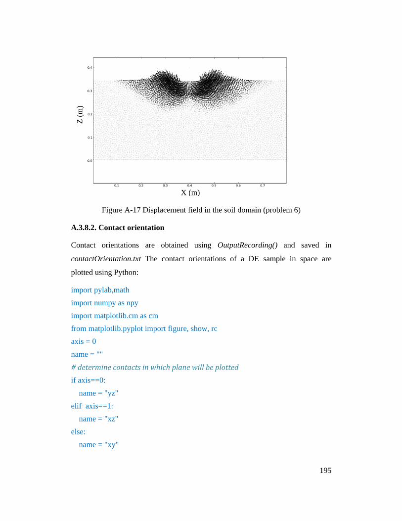
Figure A-17 Displacement field in the soil domain (problem 6)
A.3.8.2. Contact orientation
Contact orientations are obtained using OutputRecording() and saved in
contactOrientation.txt The contact orientations of a DE sample in space are
plotted using Python:
import pylab,math import numpy as npy import matplotlib.cm as cm from matplotlib.pyplot import figure, show, rc axis = 0 name = ""
# determine contacts in which plane will be plotted if axis==0: name = "yz" elif axis==1: name = "xz" else: name = "xy"
X (m)
Z (m
)
195
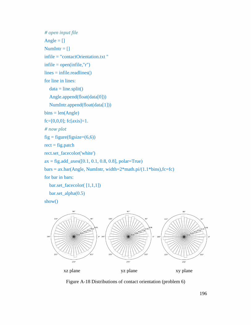
# open input file Angle = [] NumIntr = [] infile = "contactOrientation.txt " infile = open(infile,"r") lines = infile.readlines() for line in lines: data = line.split() Angle.append(float(data[0])) NumIntr.append(float(data[1])) bins = len(Angle) fc=[0,0,0]; fc[axis]=1.
# now plot fig = figure(figsize=(6,6)) rect = fig.patch rect.set_facecolor('white') ax = fig.add_axes([0.1, 0.1, 0.8, 0.8], polar=True) bars = ax.bar(Angle, NumIntr, width=2*math.pi/(1.1*bins),fc=fc) for bar in bars: bar.set_facecolor( [1,1,1]) bar.set_alpha(0.5) show()
Figure A-18 Distributions of contact orientation (problem 6)
xz plane yz plane xy plane
196
A.3.8.3. Stresses in soil
Stresses in soil can be calculated based on contact forces between DE particles. In
the framework, soil stresses are calculated using OutputRecording() and saved in
soilStress.txt. Soil stresses can be plotted using Python:
import matplotlib import numpy as np import matplotlib.cm as cm import matplotlib.mlab as mlab import matplotlib.pyplot as plt
# devide the soil domain into grids num_row x num_col num_row, num_col = 0, 0 min_X, max_X = 0.0, 0.0 min_Z, max_Z = 0.0, 0.0
# x-stresses from file sX = []
# z-stresses from file sZ = [] infile = open("soilStress.txt","r") lines = infile.readlines() count = 0 for line in lines: count += 1 data = line.split()
# first line if count == 1: num_row = float(data[0]) num_col = float(data[1]) min_X = float(data[2]) max_X = float(data[3]) min_Z = float(data[4])
197
max_Z = float(data[5]) else: sX.append(float(data[0])) sZ.append(float(data[1]))
# stresses arranged in arrays stress_X = [] stress_Z = [] count = 0 for i in range (0, num_row): stress_X.append([]) stress_Z.append([]) for j in range (0, num_col): count = i*num_col + j stress_X[i].append(sX[count]) stress_Z[i].append(sZ[count]) x = np.linspace(min_X, max_X, num_col) z = np.linspace(min_Z, max_Z, num_row) X, Z = np.meshgrid(x, z) plt.figure() CS = plt.contour(X, Z, stress_Z) plt.axis([min_X, max_X, min_Z,max_Z]) plt.clabel(CS, inline=1, fontsize=8) plt.title('Vertical stress') plt.xlabel('X (m)',size = 8) plt.ylabel('Y (m)',size = 8) plt.show()
198
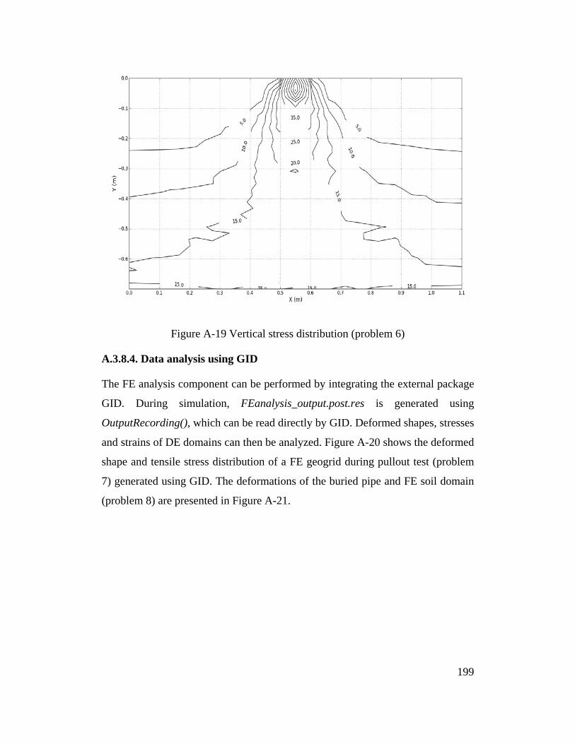
Figure A-19 Vertical stress distribution (problem 6)
A.3.8.4. Data analysis using GID
The FE analysis component can be performed by integrating the external package
GID. During simulation, FEanalysis_output.post.res is generated using
OutputRecording(), which can be read directly by GID. Deformed shapes, stresses
and strains of DE domains can then be analyzed. Figure A-20 shows the deformed
shape and tensile stress distribution of a FE geogrid during pullout test (problem
7) generated using GID. The deformations of the buried pipe and FE soil domain
(problem 8) are presented in Figure A-21.
199
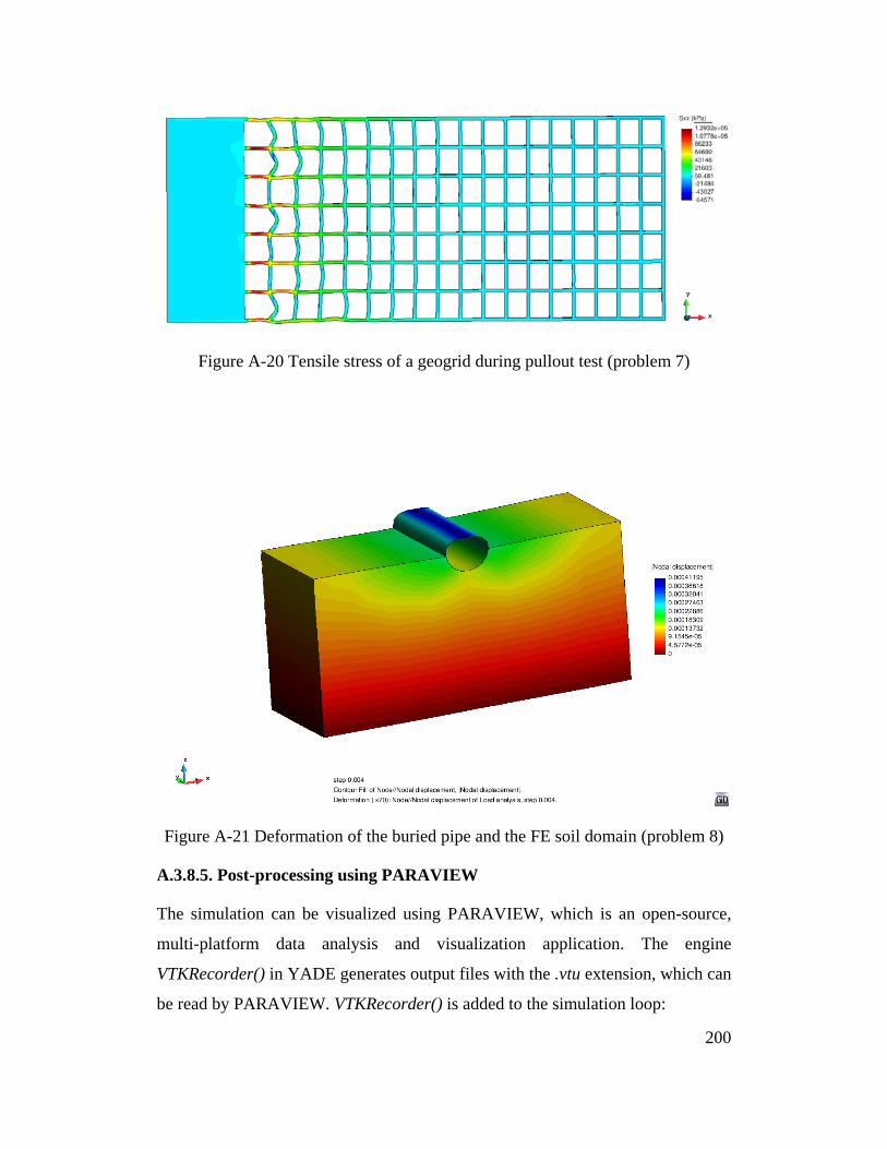
Figure A-20 Tensile stress of a geogrid during pullout test (problem 7)
Figure A-21 Deformation of the buried pipe and the FE soil domain (problem 8)
A.3.8.5. Post-processing using PARAVIEW
The simulation can be visualized using PARAVIEW, which is an open-source,
multi-platform data analysis and visualization application. The engine
VTKRecorder() in YADE generates output files with the .vtu extension, which can
be read by PARAVIEW. VTKRecorder() is added to the simulation loop:
200
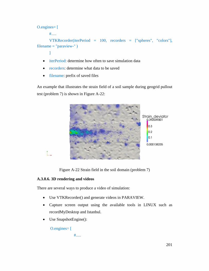
O.engines= [ #..... VTKRecorder(iterPeriod = 100, recorders = ["spheres", "colors"], filename = "paraview-" ) ]
• iterPeriod: determine how often to save simulation data
• recorders: determine what data to be saved
• filename: prefix of saved files
An example that illustrates the strain field of a soil sample during geogrid pullout
test (problem 7) is shown in Figure A-22:
Figure A-22 Strain field in the soil domain (problem 7)
A.3.8.6. 3D rendering and videos
There are several ways to produce a video of simulation:
• Use VTKRecorder() and generate videos in PARAVIEW.
• Capture screen output using the available tools in LINUX such as
recordMyDesktop and Istanbul.
• Use SnapshotEngine():
O.engines= [ #.....
201
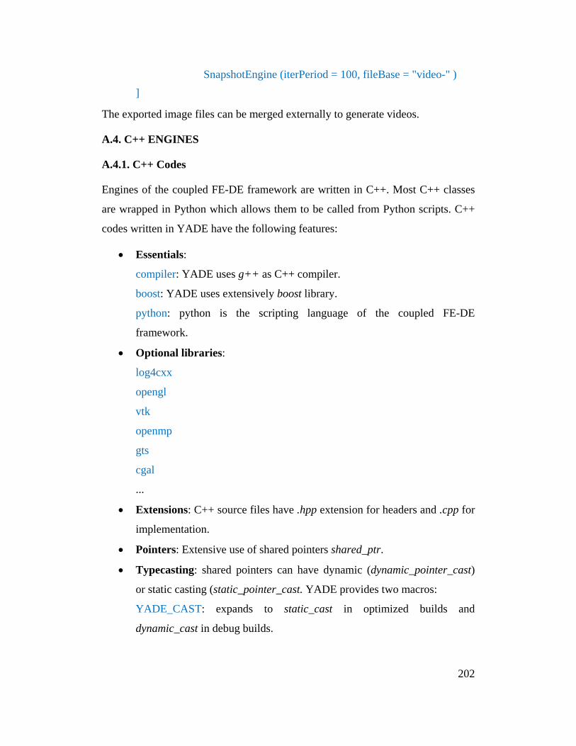
SnapshotEngine (iterPeriod = 100, fileBase = "video-" ) ]
The exported image files can be merged externally to generate videos.
A.4. C++ ENGINES
A.4.1. C++ Codes
Engines of the coupled FE-DE framework are written in C++. Most C++ classes
are wrapped in Python which allows them to be called from Python scripts. C++
codes written in YADE have the following features:
• Essentials:
compiler: YADE uses g++ as C++ compiler.
boost: YADE uses extensively boost library.
python: python is the scripting language of the coupled FE-DE
framework.
• Optional libraries:
log4cxx
opengl
vtk
openmp
gts
cgal
...
• Extensions: C++ source files have .hpp extension for headers and .cpp for
implementation.
• Pointers: Extensive use of shared pointers shared_ptr.
• Typecasting: shared pointers can have dynamic (dynamic_pointer_cast)
or static casting (static_pointer_cast. YADE provides two macros:
YADE_CAST: expands to static_cast in optimized builds and
dynamic_cast in debug builds.
202
YADE_PTR_CAST: expands to static_ptr_cast in optimized builds and
dynamic_ptr_cast in debug builds.
A.4.2. C++ Framework
• Scene: is the object containing the whole simulation. All engines and
functors have a Scene* scene pointer which assures the current scene can
be accessed from codes.
• BodyContainer: contains all bodies of a simulation. BodyContainer stores
bodies using their shared_ptr.
A new body can be inserted in C++:
scene = shared_ptr<Scene>(new Scene); shared_ptr<Body> femElement; createElement(femElement); //define element scene ->bodies->insert(femElement);
BodyContainer can be iterated using FOREACH macro:
FOREACH(const shared_ptr<Body> & body, *scene->bodies) { if (body->groupMask==1) { //do something } }
• InteractionContainer: stores interactions during simulation. Interactions
between particles are identified by a pair of ids of the two particles.
shared_ptr storage is used by InteractionContainer. Iteration over
interactions can be handled using FOREACH or:
InteractionContainer::iterator ii = scene->interactions->begin(); InteractionContainer::iterator iiEnd = scene->interactions->end(); for( ; ii!=iiEnd ; ++ii ) { if ((*ii)->isReal()) { //do something }
203
}
• ForceContainer: stores forces and torques of each body.
Adding a force to a body in C++ :
scene->forces.addForce(id, force);
Getting force acting on a body:
scene->forces.sync(); //sync before reading Vector3r f = scene->forces.getForce(id);
• Handling interactions: the following actions are performed to handle
interactions:
Potential interactions are identified using Collider.
InteractionLoop calls appropriate IGeomFunctor based on Shape of both
bodies.
InteractionLoop calls appropriate IPhysFunctor based on Material of both
bodies.
InteractionLoop calls appropriate LawFunctor based on IGeom and IPhys
of the interaction.
A.4.3. Omega Class
All simulation-related functionality is handled by Omega class. In the current
scene, Omega.materials corresponds to Scene::materials, which is the same for
bodies, interactions, engines, iter, dt, time, realtime and stopAtIter.
A.4.4. Wrapping C++ Classes
All C++ classes deriving from Serializable can be called from Python. This is
achieved via YADE_CLASS_BASE_DOC_* macro family.
204
REFERENCES
Abu-Farsakh, Murad, CHEN QIMING, Radhey Sharma, and Xiong Zhang (2008)
"Large-Scale Model Footing Tests on Geogrid-Reinforced Foundation and
Marginal Embankment Soils," ASTM geotechnical testing journal, Vol. 31,
No. 5, pp 413-423.
Adams, M.T., and Collin, J.G. (1997) "Large model spread footing load tests on
geosynthetic reinforced soil foundations," Journal of Geotechnical and
Geoenvironmental Engineering, Vol. 123, No. 1, pp 66-72.
Agaiby, Sherif W, and Colin JFP Jones (1995) "Design of reinforced fill systems
over voids," Canadian Geotechnical Journal, Vol. 32, No. 6, pp 939-945.
Alagiyawanna, AMN, M Sugimoto, S Sato, and H Toyota (2001) "Influence of
longitudinal and transverse members on geogrid pullout behavior during
deformation," Geotextiles and Geomembranes, Vol. 19, No. 8, pp 483-507.
Andresen, Lars, Hans Petter Jostad, and Knut H Andersen (2011) "Finite Element
Analyses Applied in Design of Foundations and Anchors for Offshore
Structures," International Journal of Geomechanics, Vol. 11, No. 6, pp 417-
430.
Bagi, Katalin (2006) "Analysis of microstructural strain tensors for granular
assemblies," International Journal of Solids and Structures, Vol. 43, No. 10,
pp 3166-3184.
Basudhar, PK, Santanu Saha, and Kousik Deb (2007) "Circular footings resting
on geotextile-reinforced sand bed," Geotextiles and Geomembranes, Vol. 25,
No. 6, pp 377-384.
Belheine, N, J-P Plassiard, F-V Donzé, F Darve, and A Seridi (2009) "Numerical
simulation of drained triaxial test using 3D discrete element modeling,"
Computers and Geotechnics, Vol. 36, No. 1, pp 320-331.
205
Berezantzev, V. G. (1958) "Earth pressure on the cylindrical retaining walls,"
Conference on earth pressure problems, Brussels, pp 21-27.
Bergado, Dennes T, and Jin-Chun Chai (1994) "Pullout force/displacement
relationship of extensible grid reinforcements," Geotextiles and
Geomembranes, Vol. 13, No. 5, pp 295-316.
Bfer, G (1985) "An isoparametric joint/interface element for finite element
analysis," International journal for numerical methods in engineering, Vol.
21, No. 4, pp 585-600.
Bhuvaraghan, Baskaran, Sivakumar M Srinivasan, Bob Maffeo, Robert D
McCLain, Yogesh Potdar, and Om Prakash (2010) "Shot peening simulation
using discrete and finite element methods," Advances in Engineering
Software, Vol. 41, No. 12, pp 1266-1276.
Binquet, Jean, and Kenneth L Lee (1975) "Bearing capacity analysis of reinforced
earth slabs," Journal of the geotechnical Engineering Division, Vol. 101, No.
12, pp 1257-1276.
Binquet, Jean, and Kenneth L Lee (1975) "Bearing capacity tests on reinforced
earth slabs," Journal of the geotechnical Engineering Division, Vol. 101, No.
12, pp 1241-1255.
Briancon, LAURENT, and Pascal Villard (2008) "Design of geosynthetic-
reinforced platforms spanning localized sinkholes," Geotextiles and
Geomembranes, Vol. 26, No. 5, pp 416-428.
Bridle, R.J., Jenner, C.G., and Barr, B. (1994) "Novel applications of geogrids in
areas of shallow mineworkings," 5th Int Conf on Geotextiles, Geomembranes
and Related Products, Singapore, Vol. 1, pp 297-300.
Calvetti, Francesco (2008) "Discrete modelling of granular materials and
geotechnical problems," European Journal of Environmental and Civil
Engineering, Vol. 12, No. 7-8, pp 951-965.
206
Chen, Cheng, GR McDowell, and NH Thom (2012) "Discrete element modelling
of cyclic loads of geogrid-reinforced ballast under confined and unconfined
conditions," Geotextiles and Geomembranes, Vol. 35, pp 76-86.
Chen, Q., Abu-Farsakh, M., Sharma, R., and Zhang, X. (2007) "Laboratory
investigation of behavior of foundations on geosynthetic-reinforced clayey
soil," Transportation Research Record: Journal of the Transportation
Research Board, Vol. 2004, pp 28–38.
Chen, Qiming, Murad Abu-Farsakh, and Radhey Sharma (2009) "Experimental
and Analytical studies of reinforced crushed limestone," Geotextiles and
Geomembranes, Vol. 27, No. 5, pp 357-367.
Cheng, YM, YY Hu, and WB Wei (2007) "General axisymmetric active earth
pressure by method of characteristics—theory and numerical formulation,"
International Journal of Geomechanics, Vol. 7, No. 1, pp 1-15.
Cheng, Y. M., and Hu, Y. Y. (2005) "Active earth pressure on circular shaft lining
obtained by simplified slip line solution with general tangential stress
coefficient," Chinese Journal of Geotechnical Engineering, Vol. 27, No. 1, pp
110-115.
Cheung, G. (2010) "Micromechanics of sand production in oil wells," Ph.D thesis,
Imperial College London.
Choudhary, AK, JN Jha, and KS Gill (2010) "Laboratory investigation of bearing
capacity behaviour of strip footing on reinforced flyash slope," Geotextiles
and Geomembranes, Vol. 28, No. 4, pp 393-402.
Chun, B., and Shin, Y. (2006) "Active earth pressure acting on the cylindrical
retaining wall of a shaft," South Korea Ground and Environmental
Engineering Journal, Vol. 7, No. 4, pp 15-24.
Chung, Wilson, and Giovanni Cascante (2007) "Experimental and numerical
study of soil-reinforcement effects on the low-strain stiffness and bearing
207
capacity of shallow foundations," Geotechnical and Geological Engineering,
Vol. 25, No. 3, pp 265-281.
Costa, Yuri D, Jorge G Zornberg, Benedito S Bueno, and Carina L Costa (2009)
"Failure mechanisms in sand over a deep active trapdoor," Journal of
Geotechnical and Geoenvironmental Engineering, Vol. 135, No. 11, pp 1741-
1753.
Costalonga, M.A.R. (1988) "Geogrid pull-out tests in clay," MSc. Dissertation,
The University of Alberta, Alberta, Canada.
Costalonga, M.A.R. (1990) "Geogrid pull-out tests in clay," 4th International
Conference on Geotextiles, Geomembranes and Related Products, The
Hague, The Netherlands, Vol. 2.
Cui, L, and C O'Sullivan (2006) "Exploring the macro-and micro-scale response
of an idealised granular material in the direct shear apparatus," Geotechnique,
Vol. 56, No. 7, pp 455-468.
Cui, L, C O'sullivan, and S O'neill (2007) "An analysis of the triaxial apparatus
using a mixed boundary three-dimensional discrete element model,"
Geotechnique, Vol. 57, No. 10, pp 831-844.
Cundall, Peter A, and Otto DL Strack (1979) "A discrete numerical model for
granular assemblies," Geotechnique, Vol. 29, No. 1, pp 47-65.
Dang, HK, and MA Meguid (2009) "Algorithm to generate a discrete element
specimen with predefined properties," International Journal of
Geomechanics, Vol. 10, No. 2, pp 85-91.
Dang, HK, and MA Meguid (2010) "Evaluating the performance of an explicit
dynamic relaxation technique in analyzing non-linear geotechnical
engineering problems," Computers and Geotechnics, Vol. 37, No. 1, pp 125-
131.
Dang, HK, and MA Meguid (2013) "An efficient finite–discrete element method
for quasi‐static nonlinear soil–structure interaction problems," International
208
journal for numerical and analytical methods in geomechanics, Vol. 37, No.
2, pp 130-149.
Das, BM, EC Shin, and MT Omar (1994) "The bearing capacity of surface strip
foundations on geogrid-reinforced sand and clay—a comparative study,"
Geotechnical & Geological Engineering, Vol. 12, No. 1, pp 1-14.
Dash, Sujit Kumar, NR Krishnaswamy, and K Rajagopal (2001) "Bearing
capacity of strip footings supported on geocell-reinforced sand," Geotextiles
and Geomembranes, Vol. 19, No. 4, pp 235-256.
Deluzarche, R, and B Cambou (2006) "Discrete numerical modelling of rockfill
dams," International journal for numerical and analytical methods in
geomechanics, Vol. 30, No. 11, pp 1075-1096.
Dhia, Hachmi Ben (1998) "Problèmes mécaniques multi-échelles: la méthode
Arlequin," Comptes Rendus de l'Académie des Sciences-Series IIB-
Mechanics-Physics-Astronomy, Vol. 326, No. 12, pp 899-904.
Dhia, Hashmi Ben, and Guillaume Rateau (2005) "The Arlequin method as a
flexible engineering design tool," International journal for numerical methods
in engineering, Vol. 62, No. 11, pp 1442-1462.
Duriez, J, F Darve, and F-V Donze (2011) "A discrete modeling-based
constitutive relation for infilled rock joints," International journal of rock
mechanics and mining sciences, Vol. 48, No. 3, pp 458-468.
Dyer, M.R. (1985) "Observations of the stress distribution in crushed glass with
applications to soil reinforcement," D.Phil. Thesis, University of Oxford,
Oxford, UK.
Elmekati, Ahmed, and Usama El Shamy (2010) "A practical co-simulation
approach for multiscale analysis of geotechnical systems," Computers and
Geotechnics, Vol. 37, No. 4, pp 494-503.
209
Faheem, Hamdy, Fei Cai, and Keizo Ugai (2004) "Three-dimensional base
stability of rectangular excavations in soft soils using FEM," Computers and
Geotechnics, Vol. 31, No. 2, pp 67-74.
Fakhimi, Ali (2009) "A hybrid discrete–finite element model for numerical
simulation of geomaterials," Computers and Geotechnics, Vol. 36, No. 3, pp
386-395.
Farrag, Khalid, Yalcin B Acar, and Ilan Juran (1993) "Pull-out resistance of
geogrid reinforcements," Geotextiles and Geomembranes, Vol. 12, No. 2, pp
133-159.
Finno, Richard J, J Tanner Blackburn, and Jill F Roboski (2007) "Three-
dimensional effects for supported excavations in clay," Journal of
Geotechnical and Geoenvironmental Engineering, Vol. 133, No. 1, pp 30-36.
Gabr, MA, and TJ Hunter (1994) "Stress-strain analysis of geogrid-supported
liners over subsurface cavities," Geotechnical & Geological Engineering,
Vol. 12, No. 2, pp 65-86.
Gabr, M.A., Hunter, T.J., and Collin, J.G. (1992) "Stability of geogrid-reinforced
landfill liners over sinkholes," Proceedings, Earth Reinforcement practice.
Edited by H . Ochiai, S. Hayashi and J. Otani. A.A. Balkema, pp 595-600.
Gabrieli, Fabio, Simonetta Cola, and Francesco Calvetti (2009) "Use of an up-
scaled DEM model for analysing the behaviour of a shallow foundation on a
model slope," Geomechanics and Geoengineering: An International Journal,
Vol. 4, No. 2, pp 109-122.
Gaetano, E.A. (2010) "The response of flexible pavement systems to local
deterioration of the base layer," Master thesis, McGill University.
Galli, G, ANTONIO Grimaldi, and A Leonardi (2004) "Three-dimensional
modelling of tunnel excavation and lining," Computers and Geotechnics, Vol.
31, No. 3, pp 171-183.
210
Garikipati, K.R. and Hughes, T.J.R. (1998) "A study of strain localization in a
multiple scale framework—the one dimensional problem," Comput. Methods
Appl. Mech. Eng., Vol. 159, pp 193–222.
Ghazavi, Mahmoud, and Arash Alimardani Lavasan (2008) "Interference effect of
shallow foundations constructed on sand reinforced with geosynthetics,"
Geotextiles and Geomembranes, Vol. 26, No. 5, pp 404-415.
Ghosh, Ambarish, and Utpal Dey (2009) "Bearing ratio of reinforced fly ash
overlying soft soil and deformation modulus of fly ash," Geotextiles and
Geomembranes, Vol. 27, No. 4, pp 313-320.
Giroud, JP, R Bonaparte, JF Beech, and BA Gross (1990) "Design of soil layer-
geosynthetic systems overlying voids," Geotextiles and Geomembranes, Vol.
9, No. 1, pp 11-50.
Guido, Vito A, Dong K Chang, and Michael A Sweeney (1986) "Comparison of
geogrid and geotextile reinforced earth slabs," Canadian Geotechnical
Journal, Vol. 23, No. 4, pp 435-440.
Han, Jie, Anil Bhandari, and Fei Wang (2011) "DEM analysis of stresses and
deformations of geogrid-reinforced embankments over piles," International
Journal of Geomechanics, Vol. 12, No. 4, pp 340-350.
Han, K, DRJ Owen, and D Peric (2002) "Combined finite/discrete element and
explicit/implicit simulations of peen forming process," Engineering
Computations, Vol. 19, No. 1, pp 92-118.
Herten, Markus, and Matthias Pulsfort (1999) "Determination of spatial earth
pressure on circular shaft constructions," Granular matter, Vol. 2, No. 1, pp
1-7.
Huang, CC, and FY Menq (1997) "Deep-footing and wide-slab effects in
reinforced sandy ground," Journal of Geotechnical and Geoenvironmental
Engineering, Vol. 123, No. 1, pp 30-36.
211
Huang, Ching-Chuan, and Fumio Tatsuoka (1990) "Bearing capacity of
reinforced horizontal sandy ground," Geotextiles and Geomembranes, Vol. 9,
No. 1, pp 51-82.
Hughes, Thomas JR (1995) "Multiscale phenomena: Green's functions, the
Dirichlet-to-Neumann formulation, subgrid scale models, bubbles and the
origins of stabilized methods," Computer methods in applied mechanics and
engineering, Vol. 127, No. 1, pp 387-401.
Imamura, S., Nomoto, T., Fujii, T., and Hagiwara, T. (1999) "Earth pressures
acting on a deep shaft and the movements of adjacent ground in sand,"
Proceedings of the international symposium on geotechnical aspects of
underground construction in soft ground. Tokyo, Japan: Balkema, Rotterdam,
pp 647-652.
Itasca (2004) "PFC 2D 3.10 Particle Flow Code in two dimensions, theory and
background volume (third ed.)," Minneapolis, Minnesota.
Jenck, Orianne, Daniel Dias, and Richard Kastner (2009) "Discrete element
modelling of a granular platform supported by piles in soft soil–Validation on
a small scale model test and comparison to a numerical analysis in a
continuum," Computers and Geotechnics, Vol. 36, No. 6, pp 917-927.
Jewell, R. (1980) "Some effects of reinforcement on soils," PhD. Thesis,
University of Cambridge, UK.
Jiang, MJ, JM Konrad, and S Leroueil (2003) "An efficient technique for
generating homogeneous specimens for DEM studies," Computers and
Geotechnics, Vol. 30, No. 7, pp 579-597.
Karabatakis, DA, and TN Hatzigogos (2002) "Analysis of creep behaviour using
interface elements," Computers and Geotechnics, Vol. 29, No. 4, pp 257-277.
Karthigeyan, S, VVGST Ramakrishna, and K Rajagopal (2007) "Numerical
investigation of the effect of vertical load on the lateral response of piles,"
212
Journal of Geotechnical and Geoenvironmental Engineering, Vol. 133, No. 5,
pp 512-521.
Kasper, Thomas, and Günther Meschke (2004) "A 3D finite element simulation
model for TBM tunnelling in soft ground," International journal for
numerical and analytical methods in geomechanics, Vol. 28, No. 14, pp 1441-
1460.
Khedkar, MS, and JN Mandal (2009) "Pullout behaviour of cellular
reinforcements," Geotextiles and Geomembranes, Vol. 27, No. 4, pp 262-
271.
Khing, KH, BM Das, VK Puri, EE Cook, and SC Yen (1993) "The bearing-
capacity of a strip foundation on geogrid-reinforced sand," Geotextiles and
Geomembranes, Vol. 12, No. 4, pp 351-361.
Khodair, Yasser A., and Sophia Hassiotis (2005) "Analysis of soil–pile interaction
in integral abutment," Computers and Geotechnics, Vol. 32, No. 3, pp 201-
209.
Kinney, Thomas C, and Billy Connor (1987) "Geosynthetics supporting
embankments over voids," Journal of cold regions engineering, Vol. 1, No. 4,
pp 158-170.
Konig, D., Guettler, U., and Jessberger, H. L. (1991) "Stress redistribution during
tunnel and shaft construction," Proceedings of the International Conference
Centrifuge 1991, Boulder, Colorado, pp 129-135.
Koutsabeloulis, NC, and DV Griffiths (1989) "Numerical modelling of the trap
door problem," Geotechnique, Vol. 39, No. 1, pp 77-89.
Kozicki, J, and FV Donzé (2009) "Yade-open dem: an open-source software
using a discrete element method to simulate granular material," Engineering
Computations, Vol. 26, No. 7, pp 786-805.
213
Kumar, Arvind, and Swami Saran (2003) "Bearing capacity of rectangular footing
on reinforced soil," Geotechnical & Geological Engineering, Vol. 21, No. 3,
pp 201-224.
Kurian, Nainan P, KS Beena, and R Krishna Kumar (1997) "Settlement of
reinforced sand in foundations," Journal of Geotechnical and
Geoenvironmental Engineering, Vol. 123, No. 9, pp 818-827.
Labra, Carlos, and Eugenio Onate (2009) "High‐density sphere packing for
discrete element method simulations," Communications in Numerical
Methods in Engineering, Vol. 25, No. 7, pp 837-849.
Ladd, R. S. (1978) "Preparing test specimens using undercompaction,"
Geotechnical Testing Journal, GTJODJ 1978, Vol. 1, No. 1, pp 16-23.
Lade, P. V., Jessberger, H. L., Makowski, E., and Jordan, P. (1981) "Modeling of
deep shafts in centrifuge test," Proceedings of the International Conference
on Soil Mechanics and Foundation Engineering, Stockholm, Sweden, Vol. 1,
pp 683-691.
Latha, G Madhavi, and Amit Somwanshi (2009) "Bearing capacity of square
footings on geosynthetic reinforced sand," Geotextiles and Geomembranes,
Vol. 27, No. 4, pp 281-294.
Lawson, C.R., Jones, C.J.F.P., Kempton, G.T., and Passaris, E.K.S. (1994)
"Advanced analysis of reinforced fills over areas prone to subsidence,"
Proceedings, 5th International Conference on Geotextiles, Geomembranes
and Related Products. A.A. Balkema, Singapore, Vol. 1, pp 311-317.
Li, Fu-Lin, Fang-Le Peng, Yong Tan, W Kongkitkul, and MSA Siddiquee (2012)
"FE simulation of viscous behavior of geogrid-reinforced sand under
laboratory-scale plane-strain-compression testing," Geotextiles and
Geomembranes, Vol. 31, pp 72-80.
Liu, SH, De’an Sun, and Hajime Matsuoka (2005) "On the interface friction in
direct shear test," Computers and Geotechnics, Vol. 32, No. 5, pp 317-325.
214
Lobo-Guerrero, S, and LE Vallejo (2005) "DEM analysis of crushing around
driven piles in granular materials," Geotechnique, Vol. 55, No. 8.
Lobo-Guerrero, Sebastian, and Luis E Vallejo (2006) "Discrete element method
analysis of railtrack ballast degradation during cyclic loading," Granular
matter, Vol. 8, No. 3-4, pp 195-204.
Madhavi Latha, G, and Amit Somwanshi (2009) "Effect of reinforcement form on
the bearing capacity of square footings on sand," Geotextiles and
Geomembranes, Vol. 27, No. 6, pp 409-422.
Maheshwari, BK, KZ Truman, PL Gould, and MH El Naggar (2005) "Three-
dimensional nonlinear seismic analysis of single piles using finite element
model: effects of plasticity of soil," International Journal of Geomechanics,
Vol. 5, No. 1, pp 35-44.
Maynar, Manuel J, and Luis E Rodríguez (2005) "Discrete numerical model for
analysis of earth pressure balance tunnel excavation," Journal of
Geotechnical and Geoenvironmental Engineering, Vol. 131, No. 10, pp 1234-
1242.
McDowell, G.R., Harireche, O., Konietzky, H., Brown, S.F., Thom, N.H. (2006)
"Discrete element modelling of geogrid-reinforced aggregates," Proceedings
of the ICE - Geotechnical Engineering, Vol. 159, No. 1, pp 35-48.
Meguid, MA, and HK Dang (2009) "The effect of erosion voids on existing
tunnel linings," Tunnelling and Underground Space Technology, Vol. 24, No.
3, pp 278-286.
Meguid, MA, and RK Rowe (2006) "Stability of D-shaped tunnels in a Mohr
Coulomb material under anisotropic stress conditions," Canadian
Geotechnical Journal, Vol. 43, No. 3, pp 273-281.
Meyerhof, GG, and AM Hanna (1978) "Ultimate bearing capacity of foundations
on layered soils under inclined load," Canadian Geotechnical Journal, Vol.
15, No. 4, pp 565-572.
215
Michalowski, Radoslaw L (2004) "Limit loads on reinforced foundation soils,"
Journal of Geotechnical and Geoenvironmental Engineering, Vol. 130, No. 4,
pp 381-390.
Michalowski, Radoslaw L, and Lei Shi (2003) "Deformation patterns of
reinforced foundation sand at failure," Journal of Geotechnical and
Geoenvironmental Engineering, Vol. 129, No. 5, pp 439-449.
Milligan, G.W.E., Earl, R.F., Bush, D.I. (1990) "Observations of photo-elastic
pullout tests on geotextiles and geogrids," 4th International Conference on
Geotextiles, Geomembranes and Related Products, The Hague, The
Netherlands, Vol. 2, pp 747-751.
Mohamed, MHA (2010) "Two dimensional experimental study for the behaviour
of surface footings on unreinforced and reinforced sand beds overlying soft
pockets," Geotextiles and Geomembranes, Vol. 28, No. 6, pp 589-596.
Moraci, Nicola, and Piergiorgio Recalcati (2006) "Factors affecting the pullout
behaviour of extruded geogrids embedded in a compacted granular soil,"
Geotextiles and Geomembranes, Vol. 24, No. 4, pp 220-242.
Mroueh, Hussein, and Isam Shahrour (2002) "Three‐dimensional finite element
analysis of the interaction between tunneling and pile foundations,"
International journal for numerical and analytical methods in geomechanics,
Vol. 26, No. 3, pp 217-230.
Ng, Tang-Tat (2004) "Triaxial test simulations with discrete element method and
hydrostatic boundaries," Journal of engineering mechanics, Vol. 130, No. 10,
pp 1188-1194.
O’Sullivan, C. (2011) "Particulate discrete element modeling, a geomechanics
perspective," Spon Press.
Ochiai, Hidetoshi, Jun Otani, Shigenori Hayashic, and Takao Hirai (1996) "The
pull-out resistance of geogrids in reinforced soil," Geotextiles and
Geomembranes, Vol. 14, No. 1, pp 19-42.
216
Onate, E, and J Rojek (2004) "Combination of discrete element and finite element
methods for dynamic analysis of geomechanics problems," Computer
methods in applied mechanics and engineering, Vol. 193, No. 27, pp 3087-
3128.
Osman, Ashraf S, and Mark F Randolph (2011) "Analytical Solution for the
Consolidation around a Laterally Loaded Pile," International Journal of
Geomechanics, Vol. 12, No. 3, pp 199-208.
O'Sullivan, Catherine, and Liang Cui (2009) "Micromechanics of granular
material response during load reversals: Combined DEM and experimental
study," Powder Technology, Vol. 193, No. 3, pp 289-302.
Palmeira, E.M. (1987) "The study of soil-reinforcement interaction by means of
large scale laboratory tests," DPhil. Thesis, University of Oxford, Oxford,
UK.
Palmeira, Ennio Marques (2004) "Bearing force mobilisation in pull-out tests on
geogrids," Geotextiles and Geomembranes, Vol. 22, No. 6, pp 481-509.
Palmeira, Ennio Marques (2009) "Soil–geosynthetic interaction: Modelling and
analysis," Geotextiles and Geomembranes, Vol. 27, No. 5, pp 368-390.
Pan, JL, ATC Goh, KS Wong, and AR Selby (2002) "Three‐dimensional analysis
of single pile response to lateral soil movements," International journal for
numerical and analytical methods in geomechanics, Vol. 26, No. 8, pp 747-
758.
Park, Jung-Wook, and Jae-Joon Song (2009) "Numerical simulation of a direct
shear test on a rock joint using a bonded-particle model," International
journal of rock mechanics and mining sciences, Vol. 46, No. 8, pp 1315-
1328.
Patra, CR, BM Das, M Bhoi, and EC Shin (2006) "Eccentrically loaded strip
foundation on geogrid-reinforced sand," Geotextiles and Geomembranes,
Vol. 24, No. 4, pp 254-259.
217
Poorooshasb, Hormoz B (1991) "Load settlement response of a compacted fill
layer supported by a geosynthetic overlying a void," Geotextiles and
Geomembranes, Vol. 10, No. 3, pp 179-201.
Potyondy, DO, and PA Cundall (2004) "A bonded-particle model for rock,"
International journal of rock mechanics and mining sciences, Vol. 41, No. 8,
pp 1329-1364.
Prater, EG (1977) "An examination of some theories of earth pressure on shaft
linings," Canadian Geotechnical Journal, Vol. 14, No. 1, pp 91-106.
Sadoglu, Erol, Evrim Cure, Berkan Moroglu, and Bayram Ali Uzuner (2009)
"Ultimate loads for eccentrically loaded model shallow strip footings on
geotextile-reinforced sand," Geotextiles and Geomembranes, Vol. 27, No. 3,
pp 176-182.
Salgado, R, and M Prezzi (2007) "Computation of cavity expansion pressure and
penetration resistance in sands," International Journal of Geomechanics, Vol.
7, No. 4, pp 251-265.
Schlosser, F., Jacobsen, H.M., and Juran, I. (1983) "Soil reinforcement," Genereal
Report, Eighth European Conference on Soil Mechanics and Foundation
Engineering, Balkema, Helsinki, pp 83–103.
Sharma, Radhey, Qiming Chen, Murad Abu-Farsakh, and Sungmin Yoon (2009)
"Analytical modeling of geogrid reinforced soil foundation," Geotextiles and
Geomembranes, Vol. 27, No. 1, pp 63-72.
Shin, E.C., Das, B.M., Puri, V.K., Yen, S.C., and Cook, E.E. (1993) "Bearing
capacity of strip foundation on geogrid-reinforced clay," Geotechnical
Testing Journal, ASTM, Vol. 16, No. 4, pp 534–541.
Siddiquee, MSA, and CC Huang (2001) "FEM simulation of the bearing capacity
of level reinforced sand ground subjected to footing load," Geosynthetics
International, Vol. 8, No. 6, p 501.
218
Sieira, Ana Cristina CF, Denise Gerscovich, and Alberto SFJ Sayão (2009)
"Displacement and load transfer mechanisms of geogrids under pullout
condition," Geotextiles and Geomembranes, Vol. 27, No. 4, pp 241-253.
Šmilauer, V., Catalano, E., Chareyre, B., Dorofeenko, S., Duriez, J., Gladky, A.,
Kozicki, J., Modenese, C., Scholtès, L., Sibille, L., Stránský, J., and Thoeni,
K. (2010) "Yade Documentation," The Yade Project 2010. (http://yade-
dem.org/doc/).
Sugimoto, M, and AMN Alagiyawanna (2003) "Pullout behavior of geogrid by
test and numerical analysis," Journal of Geotechnical and Geoenvironmental
Engineering, Vol. 129, No. 4, pp 361-371.
Sugimoto, M, AMN Alagiyawanna, and K Kadoguchi (2001) "Influence of rigid
and flexible face on geogrid pullout tests," Geotextiles and Geomembranes,
Vol. 19, No. 5, pp 257-277.
Tafreshi, SN, and AR Dawson (2010) "Behaviour of footings on reinforced sand
subjected to repeated loading–Comparing use of 3D and planar geotextile,"
Geotextiles and Geomembranes, Vol. 28, No. 5, pp 434-447.
Terzaghi, K. (1936) "Stress distribution in dry and saturated sand above a yielding
trap door," Proceedings, International Conference of Soil Mechanics, Harvard
University, Cambridge, Mass., Vol. 1, pp 307-311.
Terzaghi, K. (1943) "Theoretical soil mechanics," New York: John Wiley & sons
Inc.
Thornton, Colin, and Ling Zhang (2003) "Numerical simulations of the direct
shear test," Chemical engineering & technology, Vol. 26, No. 2, pp 153-156.
Tobar, T. (2009) "An experimental study of the earth pressure distribution on
cylindrical shafts," Master’s thesis, McGill University.
Tobar, Tatiana, and Mohamed A Meguid (2011) "Experimental study of the earth
pressure distribution on cylindrical shafts," Journal of Geotechnical and
Geoenvironmental Engineering, Vol. 137, No. 11, pp 1121-1125.
219
Tran, VDH, MA Meguid, and LE Chouinard (2013) "A finite–discrete element
framework for the 3D modeling of geogrid–soil interaction under pullout
loading conditions," Geotextiles and Geomembranes, Vol. 37, pp 1-9.
Tran, VDH, MA Meguid, and LE Chouinard (2013) "Three-Dimensional
Analysis of Geogrid Reinforced Soil Using Finite-Discrete Element
Framework," International Journal of Geomechanics (submitted).
Tran, VDH, MA Meguid, and LE Chouinard (2012) "Discrete Element and
Experimental Investigations of the Earth Pressure Distribution on Cylindrical
Shafts," International Journal of Geomechanics (in press).
Van Langen, H, and PA Vermeer (1991) "Interface elements for singular
plasticity points," International journal for numerical and analytical methods
in geomechanics, Vol. 15, No. 5, pp 301-315.
Villard, Pascal, and Bruno Chareyre (2004) "Design methods for geosynthetic
anchor trenches on the basis of true scale experiments and discrete element
modelling," Canadian Geotechnical Journal, Vol. 41, No. 6, pp 1193-1205.
Villard, P, B Chevalier, B Le Hello, and G Combe (2009) "Coupling between
finite and discrete element methods for the modelling of earth structures
reinforced by geosynthetic," Computers and Geotechnics, Vol. 36, No. 5, pp
709-717.
Villard, P, JP Gourc, and H Giraud (2000) "A geosynthetic reinforcement solution
to prevent the formation of localized sinkholes," Canadian Geotechnical
Journal, Vol. 37, No. 5, pp 987-999.
Walz, B. (1973) "Left bracket apparatus for measuring the three-dimensional
active soil pressure on a round model caisson right bracket," Baumaschine
und Bautechnik, Vol. 20, No. 9, pp 339-344
Wang, MC, YX Feng, and M Jao (1996) "Stability of geosynthetic-reinforced soil
above a cavity," Geotextiles and Geomembranes, Vol. 14, No. 2, pp 95-109.
220
Wayne, M.H., Han, J., and Akins, K. (1998) "The design of geosynthetic
reinforced foundations," Proceedings of ASCE’s 1998 Annual Convention &
Exposition. ASCE Geotechnical Special Publication, Vol. 76, pp 1–18.
Weatherley, D., Boros, V., and Hancock, W. (2011) "ESyS - Particle Tutorial and
User's Guide Version 2.1," The University of Queensland.
Xiao, SP, and Ted Belytschko (2004) "A bridging domain method for coupling
continua with molecular dynamics," Computer methods in applied mechanics
and engineering, Vol. 193, No. 17, pp 1645-1669.
Yamamoto, Kentaro, and Jun Otani (2002) "Bearing capacity and failure
mechanism of reinforced foundations based on rigid-plastic finite element
formulation," Geotextiles and Geomembranes, Vol. 20, No. 6, pp 367-393.
Yan, Ying, and Shunying Ji (2010) "Discrete element modeling of direct shear
tests for a granular material," International journal for numerical and
analytical methods in geomechanics, Vol. 34, No. 9, pp 978-990.
Yetimoglu, Temel, Jonathan TH Wu, and Ahmet Saglamer (1994) "Bearing
capacity of rectangular footings on geogrid-reinforced sand," Journal of
Geotechnical Engineering, Vol. 120, No. 12, pp 2083-2099.
Yoo, Chungsik (2013) "Interaction between tunneling and bridge foundation–A
3D numerical investigation," Computers and Geotechnics, Vol. 49, pp 70-78.
Zdravkovic, L, DM Potts, and HD St John (2005) "Modelling of a 3D excavation
in finite element analysis," Geotechnique, Vol. 55, No. 7, pp 497-513.
Zienkiewicz, OC, and GC Huang (1990) "A note on localization phenomena and
adaptive finite‐element analysis in forming processes," Communications in
applied numerical methods, Vol. 6, No. 2, pp 71-76.
Zienkiewicz, O. C., M. Pastor, and Mao-song Huang (1995) "Softening,
localisation and adaptive remeshing. Capture of discontinuous solutions,"
Computational mechanics, Vol. 17, No. 1-2, pp 98-106.
221
Zienkiewicz, O. C. and Huang, G. C. (1990) "A note on localization phenomena
and adaptive finite-element analysis in forming processes," Commun. appl.
numer. methods, Vol. 6, pp 71–76.
222