1

Ninth International Conference on Computational Fluid Dynamics (ICCFD9), Istanbul, Turkey, July 11-15, 2016

ICCFD9-0207

A coupled Discrete Element Method and Finite Volume Method

for the simulation of elastic fishnets in interaction with fluid. Paolo Sassi1, Jorge Freiría1 & Gabriel Usera1

1Department of Fluid Mechanics and Environmental Engineering, School of Engineering, University of the Republic, Montevideo, Uruguay

Corresponding author: gusera@fing.edu.uy

Abstract: Several devices and manmade structures interact dynamically with fluids such as water and air, behaving essentially as flexible elastic systems with large deformations and undergoing complex dynamics. The design and analysis of the configurations that these devices may acquire under different flow conditions can be carried out using numerical modeling tools. This paper presents the implementation of a Discrete Element Method (DEM) coupled with a Finite Volume Method (FVM) to represent the bi-directional dynamic interaction of flexible elastic systems with fluids, and its application to fishnets. Keywords: Computational Fluid Dynamics, Discrete Element Method, Fishnets.

1 Introduction The dynamic of fishing nets is a matter of high complexity, the fundamental reason being that the forces acting on these devices depend on their shape, and at the same time, due to the elastic nature of the materials that shape it, the form it adopts is strongly influenced by its interaction with the hydrodynamic flow and other forces. Being able to design and define the shapes that various types of fishing gear might acquire under different flow conditions, represents an important challenge in terms of energy, trading and sustainability. Improvements are needed in design configurations in order to achieve greater efficiency in fishing, allowing better gear selectivity and reducing also the hydrodynamic resistance to reduce fuel consumption [3]. There are many researches aimed at making changes in the construction of fish nets that help to improve the selectivity. Selectivity is the ability of the net to retain a target species and within it, individuals whose sizes are above the average size that define the maturity of the specimen. This ensures that young specimens can escape the device and continue to maintain the sustainability of the resource. And also ensures an improvement in the efficiency of the net from an economic standpoint and especially in environmental terms. The design and setup of fishing nets can be aided by numerical simulations of their interaction during trawling with water and free bodies dragged by the stream, with the aim of predicting the shape adopted by the fishnet and the forces exerted onto it. The Discrete Element Method (DEM) is well suited to represent elastic structures such as fishnets, while the Finite Volume Method (FVM) is widely used to simulate fluid flow. In this work we present a coupled model where a simple DEM method is implemented to represent the dynamics of the fishnet, while the fluid flow is solved using caffa3d.MBRi [6, 7], an open source fully implicit finite volume method for the 3D incompressible Navier-Stokes equations in complex geometry. Validation of the flow solver as well as mesh and time

2

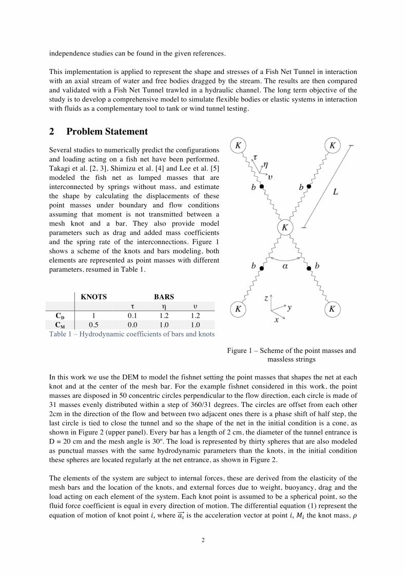
independence studies can be found in the given references. This implementation is applied to represent the shape and stresses of a Fish Net Tunnel in interaction with an axial stream of water and free bodies dragged by the stream. The results are then compared and validated with a Fish Net Tunnel trawled in a hydraulic channel. The long term objective of the study is to develop a comprehensive model to simulate flexible bodies or elastic systems in interaction with fluids as a complementary tool to tank or wind tunnel testing. 2 Problem Statement Several studies to numerically predict the configurations and loading acting on a fish net have been performed. Takagi et al. [2, 3], Shimizu et al. [4] and Lee et al. [5] modeled the fish net as lumped masses that are interconnected by springs without mass, and estimate the shape by calculating the displacements of these point masses under boundary and flow conditions assuming that moment is not transmitted between a mesh knot and a bar. They also provide model parameters such as drag and added mass coefficients and the spring rate of the interconnections. Figure 1 shows a scheme of the knots and bars modeling, both elements are represented as point masses with different parameters, resumed in Table 1.

KNOTS BARS τ η υ

CD 1 0.1 1.2 1.2 CM 0.5 0.0 1.0 1.0

Table 1 – Hydrodynamic coefficients of bars and knots

In this work we use the DEM to model the fishnet setting the point masses that shapes the net at each knot and at the center of the mesh bar. For the example fishnet considered in this work, the point masses are disposed in 50 concentric circles perpendicular to the flow direction, each circle is made of 31 masses evenly distributed within a step of 360/31 degrees. The circles are offset from each other 2cm in the direction of the flow and between two adjacent ones there is a phase shift of half step, the last circle is tied to close the tunnel and so the shape of the net in the initial condition is a cone, as shown in Figure 2 (upper panel). Every bar has a length of 2 cm, the diameter of the tunnel entrance is D = 20 cm and the mesh angle is 30º. The load is represented by thirty spheres that are also modeled as punctual masses with the same hydrodynamic parameters than the knots, in the initial condition these spheres are located regularly at the net entrance, as shown in Figure 2. The elements of the system are subject to internal forces, these are derived from the elasticity of the mesh bars and the location of the knots, and external forces due to weight, buoyancy, drag and the load acting on each element of the system. Each knot point is assumed to be a spherical point, so the fluid force coefficient is equal in every direction of motion. The differential equation (1) represent the equation of motion of knot point 𝑖, where 𝑎! is the acceleration vector at point 𝑖, 𝑀! the knot mass, 𝜌

Figure 1 – Scheme of the point masses and massless strings

3

the fluid density, 𝑉𝑜𝑙! the volume of knot 𝑖, 𝐶!" the added mass coefficient, the vectors 𝑇! , 𝑊! , 𝐵! ,𝐷! and 𝐹! are the tension, weight, buoyancy, drag force and interaction with fishing load force respectively.

𝑎! · 𝑀! + 𝜌 · 𝑉𝑜𝑙! · 𝐶!" = 𝑇! +𝑊! + 𝐵! + 𝐷! + 𝐹! (1)

On the other hand, the mesh bars are modeled as cylindrical elements and the fluid forces vary with different directions of relative fluid velocity, thus it is needed to transform the forces applied to each bar into the local system of the corresponding bar, add them and then transform again to the reference system (Figure 1 shows both coordinate systems). Equation (2) represent the equation of motion of the bar 𝑖 where 𝑻𝑴𝒊 is the transformation matrix between the reference coordinate system and the bar 𝑖 fixed coordinates, and the supra index ′ represents that the vector is in the local, body-fixed coordinates. Note that the Drag forces are calculated in the local coordinates.

𝑎′! · 𝑀! + 𝜌 · 𝑉𝑜𝑙! · 𝐶!" = 𝑇! · 𝑻𝑴𝒊 +𝑊! · 𝑻𝑴𝒊 + 𝐵! · 𝑻𝑴𝒊 + 𝐷′! · 𝑻𝑴𝒊 + 𝑭! (2)

𝑎! = 𝑻𝑴𝒊 · 𝑎′!! (3)

These equations have the position and velocity of each knot point and mesh bar implicit in the tension and drag force, so the displacement of the device is given by a system of ordinary differential equations. The equations can be solved numerically for each point, given an initial position of the net. Shimizu et al. [4] introduces a Fishing Net Shape Simulator (NaLA) that incorporates the sixth order Runge-Kutta method for solving the ordinary differential equation system to simulate a bottom gill net. We found that the fourth order Runge-Kutta method [1] gives the best performance to solve the ordinary differential equations system, in our case. Equations (4 – 7) summarize the method where 𝜙 is the vector with the velocity and position of every element of the system and 𝑓 is the vector containing the acceleration and velocity calculated with 𝜙 and the corresponding time.

𝜙!!!!

∗ = 𝜙! +∆𝑡2𝑓 𝑡!,𝜙! (4)

𝜙!!!!

∗∗ = 𝜙! +∆𝑡2𝑓 𝑡

!!!!,𝜙

!!!!

∗ (5)

𝜙!!!∗ = 𝜙! + ∆𝑡 𝑓 𝑡!!!!

,𝜙!!!!

∗∗ (6)

𝜙!!! = 𝜙! +∆𝑡6

𝑓 𝑡!,𝜙! + 2𝑓 𝑡!!!!

,𝜙!!!!

∗ + 2𝑓 𝑡!!!!

,𝜙!!!!

∗∗ + 𝑓 𝑡!!!,𝜙!!!∗ (7)

The domain of this simulation is covered by one prism block of 4 meter in the direction of the fluid (x direction) and 70 cm in y and z directions, the entrance circle of the net is set and fixed at x = 1 m and centered in y and z. The discretization grid for the flow solver is made by cubic cells of 1 cm length (400x70x70). The west boundary of the domain has inlet boundary condition where a uniform flow U=1 m/s in the x direction enters to the domain, without turbulence modeling. The east boundary is the outlet, and the rest of the boundaries, north, south, top and bottom are non-slip walls. In these conditions a time step of 0.01 second is enough to solve the flow, but not enough to solve the Fishnet with the Runge-Kutta solver. So, for every time step of the fluid solver the Runge-Kutta is executed 100 times to reach the convergence of the system. To obtain the external forces acting on the fishnet, the fluid flow properties at each time step and the location of each element of the fishnet are required in order to compute the drag forces. The velocity is obtained by a search and interpolation routine that interrogates the finite volume grid for each lumped mass location. The drag forces are then calculated and applied to both the fishnet and the

4

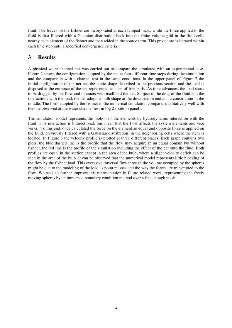
fluid. The forces on the fishnet are incorporated at each lumped mass, while the force applied to the fluid is first filtered with a Gaussian distribution back into the finite volume grid in the fluid cells nearby each element of the fishnet and then added in the source term. This procedure is iterated within each time step until a specified convergence criteria. 3 Results

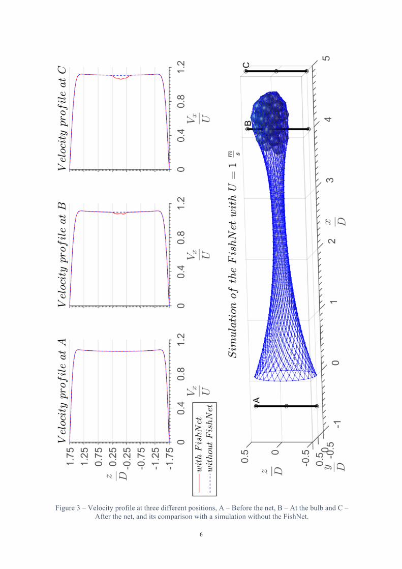
A physical water channel test was carried out to compare the simulated with an experimental case. Figure 2 shows the configuration adopted by the net at four different time steps during the simulation and the comparison with a channel test in the same conditions. In the upper panel of Figure 2 the initial configuration of the net has the conic shape described in the previous section and the load is disposed at the entrance of the net represented as a set of free balls. As time advances, the load starts to be dragged by the flow and interacts with itself and the net. Subject to the drag of the fluid and the interactions with the load, the net adopts a bulb shape at the downstream end and a constriction in the middle. The form adopted by the fishnet in the numerical simulation compares qualitatively well with the one observed at the water channel test in Fig 2 (bottom panel). The simulation model represents the motion of the elements by hydrodynamic interaction with the fluid. This interaction is bidirectional, this mean that the flow affects the system elements and vice versa. To this end, once calculated the force on the element an equal and opposite force is applied on the fluid, previously filtered with a Gaussian distribution, in the neighboring cells where the item is located. In Figure 3 the velocity profile is plotted at three different places. Each graph contains two plots, the blue dashed line is the profile that the flow may acquire in an equal domain but without fishnet, the red line is the profile of the simulation including the effect of the net onto the fluid. Both profiles are equal in the section except in the area of the bulb, where a slight velocity deficit can be seen in the area of the bulb. It can be observed that the numerical model represents little blocking of the flow by the fishnet load. This excessive traversal flow through the volume occupied by the spheres might be due to the modeling of the load as point masses and the way the forces are transmitted to the flow. We seek to further improve this representation in future related work, representing the freely moving spheres by an immersed boundary condition method over a fine enough mesh.

5

Figure 2: Fishnet shape adopted at 4 time steps of the computational simulation, t = 0, 1, 2 and 4 seconds and comparison with a water channel test (bottom).

6

Figure 3 – Velocity profile at three different positions, A – Before the net, B – At the bulb and C – After the net, and its comparison with a simulation without the FishNet.

7

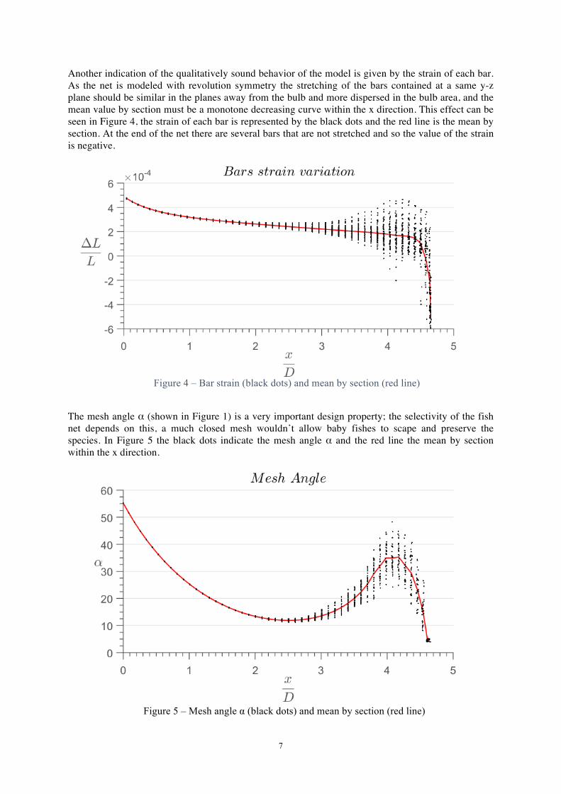
Another indication of the qualitatively sound behavior of the model is given by the strain of each bar. As the net is modeled with revolution symmetry the stretching of the bars contained at a same y-z plane should be similar in the planes away from the bulb and more dispersed in the bulb area, and the mean value by section must be a monotone decreasing curve within the x direction. This effect can be seen in Figure 4, the strain of each bar is represented by the black dots and the red line is the mean by section. At the end of the net there are several bars that are not stretched and so the value of the strain is negative.

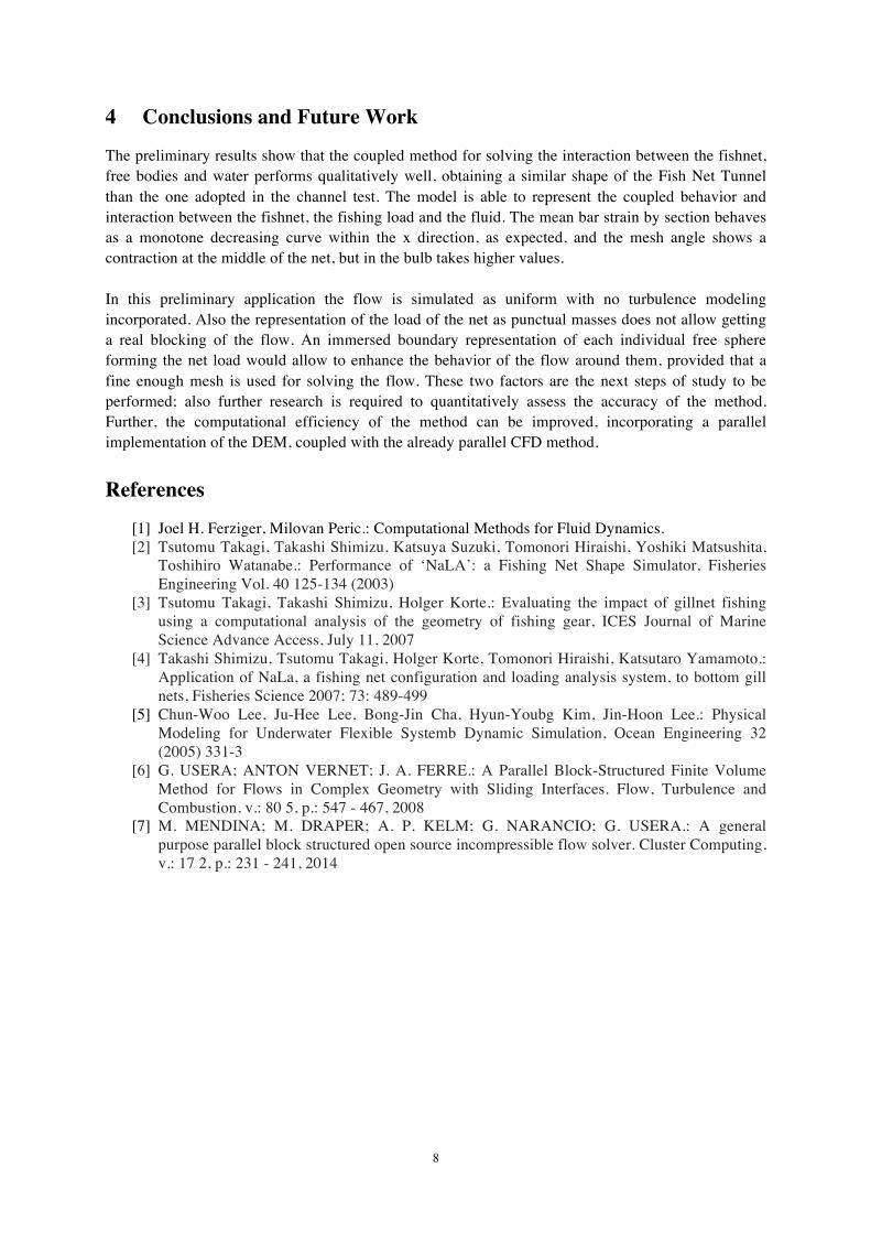
The mesh angle α (shown in Figure 1) is a very important design property; the selectivity of the fish net depends on this, a much closed mesh wouldn’t allow baby fishes to scape and preserve the species. In Figure 5 the black dots indicate the mesh angle α and the red line the mean by section within the x direction.

Figure 5 – Mesh angle α (black dots) and mean by section (red line)

Figure 4 – Bar strain (black dots) and mean by section (red line)

8

4 Conclusions and Future Work The preliminary results show that the coupled method for solving the interaction between the fishnet, free bodies and water performs qualitatively well, obtaining a similar shape of the Fish Net Tunnel than the one adopted in the channel test. The model is able to represent the coupled behavior and interaction between the fishnet, the fishing load and the fluid. The mean bar strain by section behaves as a monotone decreasing curve within the x direction, as expected, and the mesh angle shows a contraction at the middle of the net, but in the bulb takes higher values. In this preliminary application the flow is simulated as uniform with no turbulence modeling incorporated. Also the representation of the load of the net as punctual masses does not allow getting a real blocking of the flow. An immersed boundary representation of each individual free sphere forming the net load would allow to enhance the behavior of the flow around them, provided that a fine enough mesh is used for solving the flow. These two factors are the next steps of study to be performed; also further research is required to quantitatively assess the accuracy of the method. Further, the computational efficiency of the method can be improved, incorporating a parallel implementation of the DEM, coupled with the already parallel CFD method. References

[1] Joel H. Ferziger, Milovan Peric.: Computational Methods for Fluid Dynamics. [2] Tsutomu Takagi, Takashi Shimizu, Katsuya Suzuki, Tomonori Hiraishi, Yoshiki Matsushita,

Toshihiro Watanabe.: Performance of ‘NaLA’: a Fishing Net Shape Simulator, Fisheries Engineering Vol. 40 125-134 (2003)

[3] Tsutomu Takagi, Takashi Shimizu, Holger Korte.: Evaluating the impact of gillnet fishing using a computational analysis of the geometry of fishing gear, ICES Journal of Marine Science Advance Access, July 11, 2007

[4] Takashi Shimizu, Tsutomu Takagi, Holger Korte, Tomonori Hiraishi, Katsutaro Yamamoto.: Application of NaLa, a fishing net configuration and loading analysis system, to bottom gill nets, Fisheries Science 2007; 73: 489-499

[5] Chun-Woo Lee, Ju-Hee Lee, Bong-Jin Cha, Hyun-Youbg Kim, Jin-Hoon Lee.: Physical Modeling for Underwater Flexible Systemb Dynamic Simulation, Ocean Engineering 32 (2005) 331-3

[6] G. USERA; ANTON VERNET; J. A. FERRE.: A Parallel Block-Structured Finite Volume Method for Flows in Complex Geometry with Sliding Interfaces. Flow, Turbulence and Combustion, v.: 80 5, p.: 547 - 467, 2008

[7] M. MENDINA; M. DRAPER; A. P. KELM; G. NARANCIO; G. USERA.: A general purpose parallel block structured open source incompressible flow solver. Cluster Computing, v.: 17 2, p.: 231 - 241, 2014