A Convenient Category forHigher-Order Probability Theory

Chris HeunenUniversity of Edinburgh, UK

Ohad KammarUniversity of Oxford, UK

Sam StatonUniversity of Oxford, UK

Hongseok YangUniversity of Oxford, UK

Abstract—Higher-order probabilistic programminglanguages allow programmers to write sophisticatedmodels in machine learning and statistics in a succinctand structured way, but step outside the standardmeasure-theoretic formalization of probability theory.Programs may use both higher-order functions andcontinuous distributions, or even define a probabilitydistribution on functions. But standard probability the-ory cannot support higher-order functions, that is, thecategory of measurable spaces is not cartesian closed.

Here we introduce quasi-Borel spaces. We show thatthese spaces: form a new formalization of probabilitytheory replacing measurable spaces; form a cartesianclosed category and so support higher-order functions;form an extensional category and so support good proofprinciples for equational reasoning; and support con-tinuous probability distributions. We demonstrate theuse of quasi-Borel spaces for higher-order functions andprobability by: showing that a well-known constructionof probability theory involving random functions gainsa cleaner expression; and generalizing de Finetti’s the-orem, that is a crucial theorem in probability theory,to quasi-Borel spaces.

I. Introduction

To express probabilistic models in machine learning andstatistics in a succinct and structured way, it pays to usehigher-order programming languages, such as Church [16],Venture [24], or Anglican [37]. These languages supportadvanced features from both programming language the-ory and probability theory, while providing generic infer-ence algorithms for answering probabilistic queries, such asmarginalization and posterior computation, for all modelswritten in the language. As a result, the programmercan succinctly express a sophisticated probabilistic modeland explore its properties while avoiding the nontrivialbusywork of designing a custom inference algorithm.

This exciting development comes at a foundationalprice. Programs in these languages may combine higher-order functions and continuous distributions, or even de-fine a probability distribution on functions. But the stan-dard measure-theoretic formalization of probability theorycannot support higher-order functions, as the category ofmeasurable spaces is not cartesian closed [1]. For instance,the Anglican implementation of Bayesian linear regressionin Figure 1 goes beyond the standard measure-theoreticfoundation of probability theory, as it defines a probabilitydistribution on functions R→ R.

1 (let [var (/ 1 (sample (gamma 0.1 0.1)))2 mu (sample (normal 0.0 3))]3 (sample (normal mu (sqrt var))))

4 (defquery Bayesian-linear-regression

5 (let [f (let [s (sample (normal 0.0 3.0))6 b (sample (normal 0.0 3.0))]7 (fn [x] (+ (* s x) b)))]

8 (observe (normal (f 1.0) 0.5) 2.5)9 (observe (normal (f 2.0) 0.5) 3.8)

10 (observe (normal (f 3.0) 0.5) 4.5)11 (observe (normal (f 4.0) 0.5) 6.2)12 (observe (normal (f 5.0) 0.5) 8.0)

13 (predict :f f)))

Fig. 1. Bayesian linear regression in Anglican. The program definesa probability distribution on functions R → R. It first samples arandom linear function f by randomly selecting slope s and interceptb. It then adjusts the probability distribution of the function to betterdescribe five observations (1.0, 2.5), (2.0, 3.8), (3.0, 4.5), (4.0, 6.2) and(5.0, 8.0) by posterior computation. In the graph, each line has beensampled from the posterior distribution over functions.

We introduce a new formalization of probability theorythat accommodates higher-order functions. The main no-tion replacing a measurable space is a quasi-Borel space:a set X equipped with a collection of functions MX ⊆[R→ X] satisfying certain conditions (Def. 7). Intuitively,MX is the set of random variables of type X. Here R meansthat the randomness of random variables in MX comesfrom (a probability distribution on) R, one of the bestbehaving measurable spaces. Thus the primitive notionshifts from measurable subset to random variable, whichis traditionally a derived notion. For related ideas see §IX.

Quasi-Borel spaces have good properties and structure.

• The category of quasi-Borel spaces is extensional,since a morphism is just a structure-preserving func-tion (§III), and so it supports good proof principlesfor equational reasoning (in contrast to [34, §8]).

• The category of quasi-Borel spaces is cartesian closed(§IV), so that it becomes a setting to study probabil-ity distributions on higher-order functions.

• There is a natural notion of probability measure onquasi-Borel spaces (Def. 10). The space of all proba-bility measures is again a quasi-Borel space, and formsthe basis for a commutative monad on the category ofquasi-Borel spaces (§V). Thus quasi-Borel spaces formsemantics for a probabilistic programming languagein the monadic style [26].

We also illustrate the use of quasi-Borel spaces.• Bayesian regression (§VI). Quasi-Borel spaces are a

natural setting for understanding programs such asthe one in Figure 1: the prior (Lines 2–4) definesa probability distribution over functions f, i.e. ameasure on RR, and the posterior (illustrated inthe graph), is again a probability measure on RR,conditioned by the observations (Lines 5–9).

• Randomization (§VII). A key idea of categorical logicis that ∀∃ statements should become statementsabout quotients of objects. The structure of quasi-Borel spaces allows us to rephrase a crucial random-ization lemma in this way. Classically, it says that ev-ery probability kernel arises from a random function.In the setting of quasi-Borel spaces, it says that thespace of probability kernels P (R)X is a quotient ofthe space of random functions, P (RX) (Theorem 25).Notice that the higher-order structure of quasi-Borelspaces allows us to succinctly state this result.

• De Finetti’s theorem (§VIII). Probability theoristsoften encounter problems when working with arbi-trary probability measures on arbitrary measurablespaces. Quasi-Borel spaces allow us to better managethe source of randomness. For example, de Finetti’stheorem is a foundational result in Bayesian statisticswhich says that all exchangeable random sequencescan be generated from independent and identicallydistributed samples. The theorem is known to hold forstandard Borel spaces [8] or measurable spaces thatarise from good topologies [19], but not for arbitrarymeasurable spaces [9]. We show that it holds for allquasi-Borel spaces (Theorem 28).

All of this is evidence that quasi-Borel spaces form aconvenient category for higher-order probability theory.

II. Preliminaries on probability measures andmeasurable spaces

Definition 1. The Borel sets form the family ΣR of subsetsof R inductively defined as follows:• intervals (a, b) are Borel sets;• complements of Borel sets are Borel;

• countable unions of Borel sets are Borel.

The Borel sets play a crucial role in probability theorybecause of the tight connection between the notion ofprobability measure and the axiomatization of Borel sets.

Definition 2. A probability measure on R is a functionµ : ΣR → [0, 1] satisfying µ(R) = 1 and µ(

⊎Si) =

∑µ(Si)

for any countable sequence of disjoint Borel sets Si.

The natural generalization gives measurable spaces.

Definition 3. A σ-algebra on a set X is a nonemptyfamily of subsets of X that is closed under complements andcountable unions. A measurable space is a pair (X,ΣX) ofa set X and a σ-algebra ΣX on it. A probability measureon a measurable space X is a function µ : ΣX → [0, 1]satisfying µ(X) = 1 and µ(

⊎Si) =

∑µ(Si) for any

countable sequence of disjoint sets Si ∈ ΣX .

The Borel sets of the reals form a leading example of a σ-algebra. Other important examples are countable sets withtheir discrete σ-algebra, which contains all subsets. We cancharacterize these spaces as standard Borel spaces, butfirst introduce the appropriate structure-preserving maps.

Definition 4. Let (X,ΣX) and (Y,ΣY ) be measurablespaces. A measurable function f : X → Y is a functionsuch that f -1(U) ∈ ΣX when U ∈ ΣY .

Thus a measurable function f : X → Y lets us push-forward a probability measure µ on X to a probabilitymeasure f∗µ on Y by (f∗µ)(U) = µ(f -1(U)). Measurablespaces and measurable functions form a category Meas.

Real-valued measurable functions f : X → R can beintegrated with respect to a probability measure µ on(X,ΣX). The integral of a nonnegative function f is∫

X

f dµ def= supUi

∑i

(µ(Ui) · inf

x∈Ui

f(x))

,

where Ui ranges over the finite partitions of X consistingof measurable subsets. When f may be negative, theintegral of f is defined if those of min(0, f) and min(0,−f)are finite, in which case∫

X

f dµ def=(∫

X

min(0, f) dµ)−(∫

X

min(0,−f) dµ)

.

When it is convenient to make the integrated variable ex-plicit, we write

∫x∈U f(x) dµ for

∫X

(λx. f(x) · [x ∈ U ]) dµ,where U ∈ ΣX is a measurable subset and [ϕ] has thevalue 1 if ϕ holds and 0 otherwise.

A. Standard Borel spacesProposition 5 (e.g. [23], App. A1). For a measurablespace (X,ΣX) the following are equivalent:• (X,ΣX) is a retract of (R,ΣR), that is, there exist

measurable X f−→ R g−→ X such that g f = idX ;• (X,ΣX) is either measurably isomorphic to (R,ΣR) or

countable and discrete;

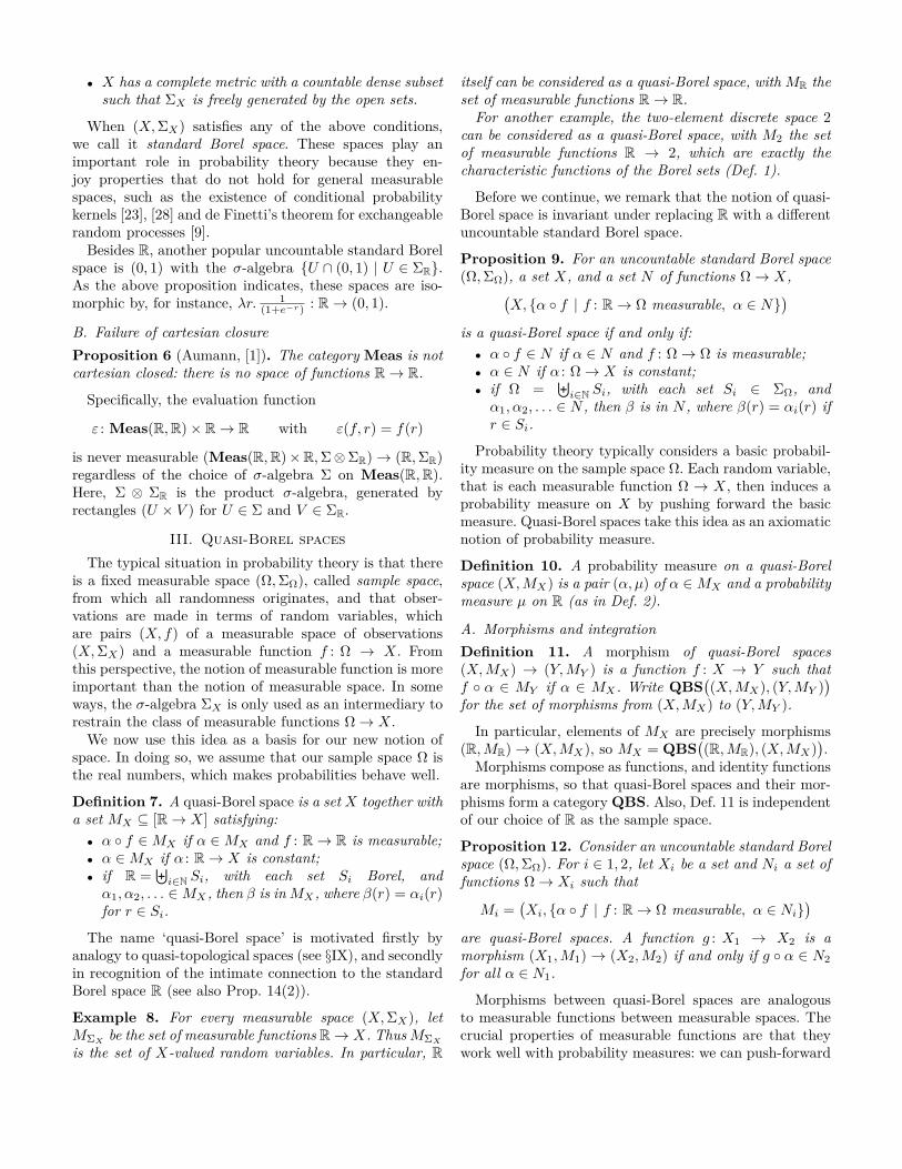
• X has a complete metric with a countable dense subsetsuch that ΣX is freely generated by the open sets.

When (X,ΣX) satisfies any of the above conditions,we call it standard Borel space. These spaces play animportant role in probability theory because they en-joy properties that do not hold for general measurablespaces, such as the existence of conditional probabilitykernels [23], [28] and de Finetti’s theorem for exchangeablerandom processes [9].

Besides R, another popular uncountable standard Borelspace is (0, 1) with the σ-algebra U ∩ (0, 1) | U ∈ ΣR.As the above proposition indicates, these spaces are iso-morphic by, for instance, λr. 1

(1+e−r) : R→ (0, 1).

B. Failure of cartesian closureProposition 6 (Aumann, [1]). The category Meas is notcartesian closed: there is no space of functions R→ R.

Specifically, the evaluation function

ε : Meas(R,R)× R→ R with ε(f, r) = f(r)

is never measurable (Meas(R,R)×R,Σ⊗ΣR)→ (R,ΣR)regardless of the choice of σ-algebra Σ on Meas(R,R).Here, Σ ⊗ ΣR is the product σ-algebra, generated byrectangles (U × V ) for U ∈ Σ and V ∈ ΣR.

III. Quasi-Borel spacesThe typical situation in probability theory is that there

is a fixed measurable space (Ω,ΣΩ), called sample space,from which all randomness originates, and that obser-vations are made in terms of random variables, whichare pairs (X, f) of a measurable space of observations(X,ΣX) and a measurable function f : Ω → X. Fromthis perspective, the notion of measurable function is moreimportant than the notion of measurable space. In someways, the σ-algebra ΣX is only used as an intermediary torestrain the class of measurable functions Ω→ X.

We now use this idea as a basis for our new notion ofspace. In doing so, we assume that our sample space Ω isthe real numbers, which makes probabilities behave well.

Definition 7. A quasi-Borel space is a set X together witha set MX ⊆ [R→ X] satisfying:• α f ∈MX if α ∈MX and f : R→ R is measurable;• α ∈MX if α : R→ X is constant;• if R =

⊎i∈N Si, with each set Si Borel, and

α1, α2, . . . ∈MX , then β is in MX , where β(r) = αi(r)for r ∈ Si.

The name ‘quasi-Borel space’ is motivated firstly byanalogy to quasi-topological spaces (see §IX), and secondlyin recognition of the intimate connection to the standardBorel space R (see also Prop. 14(2)).

Example 8. For every measurable space (X,ΣX), letMΣX

be the set of measurable functions R→ X. Thus MΣX

is the set of X-valued random variables. In particular, R

itself can be considered as a quasi-Borel space, with MR theset of measurable functions R→ R.

For another example, the two-element discrete space 2can be considered as a quasi-Borel space, with M2 the setof measurable functions R → 2, which are exactly thecharacteristic functions of the Borel sets (Def. 1).

Before we continue, we remark that the notion of quasi-Borel space is invariant under replacing R with a differentuncountable standard Borel space.

Proposition 9. For an uncountable standard Borel space(Ω,ΣΩ), a set X, and a set N of functions Ω→ X,(

X, α f | f : R→ Ω measurable, α ∈ N)

is a quasi-Borel space if and only if:• α f ∈ N if α ∈ N and f : Ω→ Ω is measurable;• α ∈ N if α : Ω→ X is constant;• if Ω =

⊎i∈N Si, with each set Si ∈ ΣΩ, and

α1, α2, . . . ∈ N , then β is in N , where β(r) = αi(r) ifr ∈ Si.

Probability theory typically considers a basic probabil-ity measure on the sample space Ω. Each random variable,that is each measurable function Ω → X, then induces aprobability measure on X by pushing forward the basicmeasure. Quasi-Borel spaces take this idea as an axiomaticnotion of probability measure.

Definition 10. A probability measure on a quasi-Borelspace (X,MX) is a pair (α, µ) of α ∈MX and a probabilitymeasure µ on R (as in Def. 2).

A. Morphisms and integrationDefinition 11. A morphism of quasi-Borel spaces(X,MX) → (Y,MY ) is a function f : X → Y such thatf α ∈ MY if α ∈ MX . Write QBS

((X,MX), (Y,MY )

)for the set of morphisms from (X,MX) to (Y,MY ).

In particular, elements of MX are precisely morphisms(R,MR)→ (X,MX), so MX = QBS

((R,MR), (X,MX)

).

Morphisms compose as functions, and identity functionsare morphisms, so that quasi-Borel spaces and their mor-phisms form a category QBS. Also, Def. 11 is independentof our choice of R as the sample space.

Proposition 12. Consider an uncountable standard Borelspace (Ω,ΣΩ). For i ∈ 1, 2, let Xi be a set and Ni a set offunctions Ω→ Xi such that

Mi =(Xi, α f | f : R→ Ω measurable, α ∈ Ni

)are quasi-Borel spaces. A function g : X1 → X2 is amorphism (X1,M1) → (X2,M2) if and only if g α ∈ N2for all α ∈ N1.

Morphisms between quasi-Borel spaces are analogousto measurable functions between measurable spaces. Thecrucial properties of measurable functions are that theywork well with probability measures: we can push-forward

these measures, and integrate over them. Morphisms ofquasi-Borel spaces also support these constructions.• Pushing forward: if f : X → Y is a morphism and

(α, µ) is a probability measure on X then f α isby definition in MY and so (f α, µ) is a probabilitymeasure on Y .

• Integrating: If f : X → R is a morphism of quasi-Borelspaces and (α, µ) is a probability measure on X, theintegral of f with respect to (α, µ) is∫

f d(α, µ) def=∫R

(f α) dµ. (1)

So integration formally reduces to integration on R.

B. Relationship to measurable spacesIf we regard a subset S ⊆ X as its characteristic function

χS : X → 2, then we can regard a σ-algebra on a set X asa set of characteristic functions FX ⊆ [X → 2] satisfyingcertain conditions. Thus a measurable space (Def. 3) couldequivalently be described as a pair (X,FX) of a set X anda collection FX ⊆ [X → 2] of characteristic functions.Moreover, from this perspective, a measurable functionf : (X,FX) → (Y, FY ) is simply a function f : X → Ysuch that χ f ∈ FX if χ ∈ FY . Thus quasi-Borel spacesshift the emphasis from characteristic functions X → 2 torandom variables R→ X.

1) Quasi-Borel spaces as structured measurable spaces:A subset S ⊆ X is in the σ-algebra ΣX of a measurablespace (X,ΣX) if and only if its characteristic functionX → 2 is measurable. With this in mind, we define ameasurable subset of a quasi-Borel space (X,MX) to be asubset S ⊆ X such that the characteristic function X → 2is a morphism of quasi-Borel spaces.

Proposition 13. The collection of all measurable subsetsof a quasi-Borel space (X,MX) is characterized as

ΣMX

def= U | ∀α ∈MX . α-1(U) ∈ ΣR (2)

and forms a σ-algebra.

Thus we can understand a quasi-Borel space as a mea-surable space (X,ΣX) equipped with a class of measurablefunctions MX ⊆ [R → X] generating the σ-algebra byΣX = ΣMX

as in (2).Moreover, every morphism (X,MX) → (Y,MY ) is also

a measurable function (X,ΣMX) → (Y,ΣMY

) (but theconverse does not hold in general).

A probability measure (α, µ) on a quasi-Borel space(X,MX) induces a probability measure α∗µ on the un-derlying measurable space. Integration as in (1) matchesthe standard definition for measurable spaces.

2) An adjunction embedding standard Borel spaces: Un-der some circumstances morphisms of quasi-Borel spacescoincide with measurable functions.

Proposition 14. Let (Y,ΣY ) be a measurable space.

1) If (X,MX) is a quasi-Borel space, a function X → Yis a measurable function (X,ΣMX

)→ (Y,ΣY ) if andonly if it is a morphism (X,MX)→ (Y,MΣY

).2) If (X,ΣX) is a standard Borel space, a function X →

Y is a morphism (X,MΣX)→ (Y,MΣY

) if and onlyif it is a measurable function (X,ΣX)→ (Y,ΣY ).

Proposition 14(1) means there is an adjunction

MeasR

22 QBSL

⊥rr

where L(X,MX) = (X,ΣMX) and R(X,ΣX) = (X,MΣX

).Proposition 14(2) means that the functor R is full andfaithful when restricted to standard Borel spaces. Equiv-alently, L(R(X,ΣX)) = (X,ΣX), that is ΣX = ΣMΣX

forstandard Borel spaces (X,ΣX).

IV. Products, coproducts and function spacesQuasi-Borel spaces support products, coproducts, and

function spaces. These basic constructions form the basisfor interpreting simple type theory in quasi-Borel spaces.

Proposition 15 (Products). If (Xi,MXi)i∈I is a family ofquasi-Borel spaces indexed by a set I, then (

∏iXi,MΠiXi

)is a quasi-Borel space, where

∏iXi is the set product, and

MΠiXi

def=f : R→

∏iXi | ∀i. (πi f) ∈MXi

.

The projections∏iXi → Xi are morphisms, and provide

the structure of a categorical product in QBS.

Proposition 16 (Coproducts). If (Xi,MXi)i∈I is a familyof quasi-Borel spaces indexed by a countable set I, then(∐iXi,MqiXi

) is a quasi-Borel space, where∐iXi is the

disjoint union of sets,

MqiXi

def= λr. (f(r), αf(r)(r)) | f : R→ I is measurable,(αi ∈MXi

)i∈image(f),

and I carries the discrete σ-algebra. This space has theuniversal property of a coproduct in the category QBS.

Proof notes. The third condition of quasi-Borel spaces isneeded here. It is a crucial step in showing that for anI-indexed family of morphisms (fi : Xi → Z)i∈I , thecopairing [fi]i∈I :

∐i∈I Xi → Z is again a morphism.

Proposition 17 (Function spaces). If (X,MX) and(Y,MY ) are quasi-Borel spaces, so is (Y X ,MY X ), whereY X

def= QBS(X,Y ) is the set of morphisms X → Y , and

MY Xdef= α : R→ Y X | uncurry(α) ∈ QBS(R×X,Y ).

The evaluation function Y X ×X → Y is a morphism andhas the universal property of the function space. Thus QBSis a cartesian closed category.

Proof notes. The only difficult part is showing that(Y X ,MY X ) satisfies the third condition of quasi-Borelspaces. Prop. 16 is useful here.

A. Relationship with standard Borel spacesRecall that standard Borel spaces can be thought of as

a full subcategory of the quasi-Borel spaces, that is, thefunctor R : Meas→ QBS is full and faithful (Prop. 14(2))when restricted to the standard Borel spaces. This fullsubcategory has the same countable products, coproductsand function spaces (whenever they exist). We may thusregard quasi-Borel spaces as a conservative extension ofstandard Borel spaces that supports simple type theory.

Proposition 18. The functor R(X,ΣX) = (X,MΣX):

1) preserves products of standard Borel spaces:R(∏iXi) =

∏iR(Xi), where (Xi,ΣXi

)i∈I is acountable family of standard Borel spaces;

2) preserves spaces of functions between standard Borelspaces whenever they exist: if (Y,ΣY ) is countableand discrete, and (X,ΣX) is standard Borel, thenR(XY ) = R(X)R(Y );

3) preserves coproducts of standard Borel spaces:R(∐iXi) =

∐iR(Xi), where (Xi,ΣXi

)i∈I is acountable family of standard Borel spaces.

Consequently, a standard programming language se-mantics in standard Borel spaces can be conservativelyembedded in quasi-Borel spaces, allowing higher-orderfunctions while preserving all the type theoretic structure.

We note, however, that in light of Prop. 6, the quasi-Borel space RR does not come from a standard Borel space.Moreover, the left adjoint L : QBS→Meas does not pre-serve products in general. For quasi-Borel spaces (X,MX)and (Y,MY ), we always have ΣMX

⊗ΣMY⊆ ΣMX×Y

, butnot always ⊇. Indeed, ΣMRR

⊗ΣR 6= ΣM(RR×R), by Prop. 6.

V. A monad of probability measuresIn this section we will show that the probability mea-

sures on a quasi-Borel space form a quasi-Borel spaceagain. This gives a commutative monad that generalizesthe Giry monad for measurable spaces [15].

A. MonadsWe use the Kleisli triple formulation of monads (see

e.g. [26]). Recall that a monad on a category C comprises• for any object X, an object T (X);• for any object X, a morphism η : X → T (X);• for any objects X,Y , a function

(>>=) : C(X,T (Y ))→ C(T (X), T (Y )).

We write (t>>=f) for (>>=)(f)(t).This is subject to the conditions (t>>=η) = t, (η(x)>>=f) =f(x), and t >>= (λx. (f(x) >>= g)) = (t >>= f) >>= g.

The intuition is that T (X) is an object of computationsreturning X, that η is the computation that returnsimmediately, and that t>>=f sequences computations, firstrunning computation t and then calling f with the result.

When C is cartesian closed, a monad is strong if (>>=) in-ternalizes to an operation (>>=) : (T (Y ))X → (T (Y ))T (X),

and then the conditions are understood as expressions ina cartesian closed category.

B. Kernels and the Giry monadWe recall the notion of probability kernel, which is a

measurable family of probability measures.

Definition 19. Let (X,ΣX) and (Y,ΣY ) be measurablespaces. A probability kernel from X to Y is a functionk : X ×ΣY → [0, 1] such that k(x,−) is a probability mea-sure for all x ∈ X (Def. 3), and k(−, U) is a measurablefunction for all U ∈ ΣY (Def. 4).

We can classify probability kernels as follows. LetG(X) be the set of probability measures on (X,ΣX).We can equip this set with the σ-algebra generated byµ ∈ G(X) | µ(U) < r, for U ∈ ΣX and r ∈ [0, 1], to forma measurable space (G(X),ΣG(X)). A measurable functionX → G(Y ) amounts to a probability kernel from X to Y .

The construction G has the structure of a monad, asfirst discussed by Giry and Lawvere [15]. A computationalintuition is that G(X) is a space of probabilistic compu-tations over X, and this provides a semantic foundationfor a first-order probabilistic programming language (seee.g. [34]). The unit η : X → G(X) lets η(x) be the Diracmeasure on x, with η(x)(U) = 1 if x ∈ U , and η(x)(U) = 0if x 6∈ U . If µ ∈ G(X) and k is a measurable functionX → G(Y ), then (µ>>=Gk) is the measure in G(Y ) with(µ>>=Gk)(U) =

∫x∈X k(x)(U) dµ.

C. Equivalent measures on quasi-Borel spacesRecall (Def. 10) that a probability measure (α, µ) on a

quasi-Borel space (X,MX) is a pair (α, µ) of a functionα ∈ MX and a probability measure µ on R. Randomvariables are often equated when they describe the samedistribution. Every probability measure (α, µ) determinesa push-forward measure α∗µ on the corresponding mea-surable space (X,ΣMX

), that assigns to U ⊆ X the realnumber µ(α−1(U)). We will identify two probability mea-sures when they define the same push-forward measure,and write ∼ for this equivalence relation.

This is a reasonable notion of equality even if weput aside the notion of measurable space, because twoprobability measures have the same push-forward measureprecisely when they have the same integration operator:(α, µ) ∼ (α′, µ′) if and only if

∫f d(α, µ) =

∫f d(α′, µ′)

for all morphisms f : (X,MX)→ R.

D. A probability monadWe now explain how to build a monad of probability

measures on the category of quasi-Borel spaces, modulothis notion of equivalence. This monad P will inheritproperties from the Giry monad. Technically, the functorL : QBS → Meas (Prop. 14) is a ‘monad opfunctor’taking P to the Giry monad G, which means that itextends to a functor from the Kleisli category of P to theKleisli category of G [36].

a) On objects: For a quasi-Borel space (X,MX), let

P (X) = (α, µ) probability measure on (X,MX)/ ∼ ,MP (X) = β : R→ P (X) | ∃α ∈MX .∃g ∈Meas(R, G(R)).

∀r ∈ R. β(r) = [α, g(r)].

Note that

P (X) ∼= α∗µ ∈ G(X,ΣMX) | α ∈MX , µ ∈ G(R) (3)

so lX([α, µ]) = α∗µ defines a measurable injectionlX : L(P (X)) G(X,ΣMX

).b) Monad unit (return): Recall that the constant

functions (λr.x) are all in MX . For any measure µ on R,the push-forward measure (λr.x)∗ µ on (X,ΣMX

) is theDirac measure on x, with ((λr.x)∗ µ)(U) = 1 if x ∈ U and0 otherwise. Thus (λr.x, µ) ∼ (λr.x, µ′) for all measuresµ, µ′ on R. The unit of P at (X,MX) is the morphismη : X → P (X) given by

η(X,MX)(x) = [λr.x, µ] (4)

for an arbitrary measure µ on R.c) Bind: To define (>>=) : P (Y )X → (P (Y ))P (X), sup-

pose f : X → P (Y ) is a morphism and [α, µ] in P (X).Since f is a morphism, there is a measurable g : R→ G(R)and a function β ∈ MY such that (f α)(r) = [β, g(r)].Set ([α, µ] >>= f) = [β, µ >>=G g], where µ >>=G g is the bindof the Giry monad. This matches the bind of the Girymonad, since ((α∗µ) >>=G (lY f)) = β∗(µ >>=G g).

Theorem 20. The data (P, η, (>>=)) above defines a strongmonad on the category QBS of quasi-Borel spaces.

Proof notes. The monad laws can be reduced to the lawsfor the monad G on Meas [15]. The monad on QBSis strong because (>>=) : P (Y )X → (P (Y ))P (X) is a mor-phism, which is shown by expanding the definitions.

Proposition 21. The monad P satisfies these properties:1) For f : (X,MX) → (Y,MY ), the functorial action

P (f) : P (X)→ P (Y ) is [α, µ] 7→ [f α, µ].2) It is a commutative monad, i.e. the order of sequenc-

ing doesn’t matter: if p ∈ P (X), q ∈ P (Y ), and f isa morphism X × Y → P (Z), then p >>= λx. q >>=λy. f(x, y) equals q >>= λy. p >>= λx. f(x, y).

3) The faithful functor L : QBS→Meas withL(X,MX) = (X,ΣMX

) extends to a faithfulfunctor Kleisli(P )→ Kleisli(G), i.e. (L, l) is a monadopfunctor [36].

4) When (X,ΣX) is a standard Borel space, the map lXof Eq. (3) is a measurable isomorphism.

VI. Example: Bayesian regressionWe are now in a position to explain the semantics of

the Anglican program in Figure 1. The program can besplit into three parts: a prior, a likelihood, and a posterior.Recall that Bayes’ law says that the posterior is propor-tionate to the product of the prior and the posterior.

Fig. 2. Illustration of 1000 sampled functions from the prior on RR

for Bayesian linear regression (5).

a) Prior: Lines 2–4 define a prior measure on RR:

prior def= (let [s (sample (normal 0.0 3.0))b (sample (normal 0.0 3.0))]

(fn [x] (+ (* s x) b)))

To describe this semantically, observe the following.

Proposition 22. Let (Ω,ΣΩ) be a standard Borel space,and (X,MX) a quasi-Borel space. Let α : R(Ω,ΣΩ) → Xbe a morphism and µ a probability measure on (Ω,ΣΩ).Any section-retraction pair (Ω ς−→ R ρ−→ Ω) = idΩ has aprobability measure [αρ, ς∗µ] ∈ P (X), that is independentof the choice of ς and ρ.

Write [α, µ] for the probability measure in this case.Now, the program fragment prior describes the distribu-

tion [α, ν⊗ν] in P (RR) where ν is the normal distributionon R with mean 0 and standard deviation 3, and whereα : R×R→ RR is given by α(s, b) def= λr. s·r+b. Informally,

JpriorK = [α, ν ⊗ ν] ∈ P (RR). (5)

Figure 2 illustrates this measure [α, ν ⊗ ν]. This deno-tational semantics can be made compositional, by usingthe commutative monad structure of P and the cartesianclosed structure of the category QBS (following e.g. [26],[34]), but in this paper we focus on this example ratherthan spelling out the general case once again.

b) Likelihood: Lines 5–9 define the likelihood of theobservations:

obs def= (observe (normal (f 1.0) 0.5) 2.5)

. . . (observe (normal (f 5.0) 0.5) 8.0)

This program fragment has a free variable f of type RR.Let us focus on line 5 for a moment:

obs1def= (observe (normal (f 1.0) 0.5) 2.5)

Given a function f : R→ R, the likelihood of drawing 2.5from a normal distribution with mean f(1.0) and standarddeviation 0.5 is

Jf : RR ` obs1K = d(f(1.0), 2.5),

where d : R2 → [0,∞) is the density of the normaldistribution function with standard deviation 0.5:

d(µ, x) =√

2π e−2(x−µ)2

.

Notice that we use a normal distribution to allow for somenoise in the measurement. Informally, we are not recordingan observation that f(1.0) is exactly 2.5, since this wouldmake regression impossible; rather, f(1.0) is roughly 2.5.

Overall, lines 5–9 describe a likelihood weight which isthe product of the likelihoods of the five data points, givenf : RR.

Jf : RR ` obsK = d(f(1), 2.5) · d(f(2), 3.8) · d(f(3), 4.5)· d(f(4), 6.2) · d(f(5), 8.0).

c) Posterior: We follow the recipe for a semanticposterior given in [34]. Putting the prior and likelihood to-gether gives a probability measure in P (RR×[0,∞)) whichis found by pushing forward the measure JpriorK ∈ P (R)along the function (id , JobsK) : RR → RR × [0,∞). Thispush-forward measure

P (id , JobsK) (JpriorK) ∈ P (RR × [0,∞))

is a measure over pairs (f, w) of functions together withtheir likelihood weight. We now find the posterior bymultiplying the prior and the likelihood, and dividing bya normalizing constant. To do this we define a morphismnorm : P (X × [0,∞))→ P (X) ] error by

norm([(α, β), ν]) def=

[α, νβ/(νβ(R))] if 0 6= νβ(R) 6=∞error otherwise

where νβ : ΣR → [0,∞] def= λU.∫r∈U (β(r)) dν. The idea is

that if β : R → [0,∞) and ν is a probability measure onR then νβ is always a posterior measure on R, but it istypically not normalized, i.e. νβ(R) 6= 1. We normalize itby dividing by the normalizing constant, as long as thisdivision is well-defined.

Now, the semantics of the entire program in Figure 1is norm(P (id , JobsK) (JpriorK)), which is a measure inP (RR). Calculating this posterior using Anglican’s infer-ence algorithm lmh gives the plot in the lower half ofFigure 1.

d) Defunctionalized regression and non-linear regres-sion: Of course, one can do regression without explicitlyconsidering distributions over the space of all measurablefunctions, by instead directly calculating posterior distri-butions for the slope s and the intercept b. For example,one could defunctionalize the program in Fig. 1 in thestyle of Reynolds [29]. But defunctionalization is a whole-program transformation. By structuring the semanticsusing quasi-Borel spaces, we are able to work composition-ally, without mentioning s and b explicitly on lines 5–10.The internal posterior calculations actually happen at thelevel of standard Borel spaces, and so a defunctionalizedversion would be in some sense equivalent, but from the

programming perspective it helps to abstract away fromthis. The regression program in Fig. 1 is quickly adaptedto fit other kinds of functions, e.g. polynomials, or evenprograms from a small domain-specific language, simplyby changing the prior in Lines 2–4.

VII. Random functionsWe discuss random variables and random functions,

starting from the traditional setting. Let (Ω,ΣΩ) be ameasurable space with a probability measure. A randomvariable is a measurable function (Ω,ΣΩ) → (X,ΣX). Arandom function between measurable spaces (X,ΣX) and(Y,ΣY ) is a measurable function (Ω × X,ΣΩ ⊗ ΣX) →(Y,ΣY ).

We can push forward a probability measure on Ω alonga random variable (Ω,ΣΩ)→ (X,ΣX) to get a probabilitymeasure on X, but in the traditional setting we cannotpush forward a measure along a random function. Mea-surable spaces are not cartesian closed (Prop. 6), and sowe cannot form a measurable space Y X and we cannotcurry a random function in general.

Now, if we revisit these definitions in the setting ofquasi-Borel spaces, we do have function spaces, and so wecan push forward along random functions. In fact, thisis somewhat tautologous because a probability measure(Def. 10) on a function space is essentially the same thingas random function: a probability measure on a functionspace (Y,ΣY )(X,ΣX) is defined to be a pair (f, µ) of aprobability measure µ on R, our sample space, and amorphism f : R→ Y X ; but to give a morphism R→ Y X

is to give a morphism R × X → Y (Prop. 17) as in thetraditional definition of random function.

We have already encountered an example of a randomfunction in Section VI: the prior for linear regression is arandom function from R to R over the measurable space(R× R,ΣR ⊗ ΣR) with the measure ν ⊗ ν. Random func-tions abound throughout probability theory and stochasticprocesses. The following section explores their use in theso-called randomization lemma, which is used throughoutprobability theory. By moving to quasi-Borel spaces, wecan state this lemma succinctly (Theorem 25).

A. RandomizationAn elementary but useful trick in probability theory is

that every probability distribution on R arises as a push-forward of the uniform distribution on [0, 1]. Even moreuseful is that this can be done in a parameterized way.

Proposition 23 ([23], Prop. 3.22). Let (X,ΣX) bea measurable space. For any kernel k : X × ΣR → [0, 1]there is a measurable function f : R×X → R such thatk(x, U) = υr | f(r, x) ∈ U, where υ is the uniform dis-tribution on [0, 1].

For quasi-Borel spaces we can phrase this more suc-cinctly: it is a result about a quotient of the space ofrandom functions. We first define quotient spaces.

Proposition 24. Let (X,MX) be a quasi-Borel space, letY be a set, and let q : X → Y be a surjection. Then (Y,MY )is a quasi-Borel space with MY = q α | α ∈MX.

We call such a space a quotient space.

Theorem 25. Let (X,MX) be a quasi-Borel space. Thespace (P (R))X of kernels is a quotient of the space P (RX)of random functions.

Before proving this theorem, we use Prop. 23 to give analternative characterization of our probability monad.

Lemma 26. Let (X,MX) be a quasi-Borel space. Thefunction q : XR → P (X) given by q(α) def= [α, υ] is a sur-jection, with corresponding quotient space (P (X),MP (X)):

MP (X) = λr ∈ R. [γ(r), υ] | γ ∈MXR, (6)

where υ is the uniform distribution on [0, 1].

Proof notes. The direction (⊆) follows immediately fromProp. 23. For the direction (⊇) we must consider γ ∈MXR

and show that (λr ∈ R. [γ(r), υ]) is in MP (X). This followsby considering the kernel k : R → G(R × R) with k(r) =υ ⊗ δr, so that [γ(r), υ] = [uncurry(γ), k(r)]. Here we areusing Prop. 22.

Proof of Theorem 25. Consider the evident morphismq : P (RX) → (P (R))X that comes from the monadicstrength. That is, (q([α, µ]))(x) = [λr. α(r)(x), µ]. Weshow that q is a quotient morphism.

We first show that q is surjective. To give a morphismk : (X,MX) → P (R) is to give a measurable function(X,ΣMX

)→ G(R), since (P (R),MP (R)) ∼= (G(R),MΣG(R))(Prop. 4(4)) and by using the adjunction between measur-able spaces and quasi-Borel spaces (Prop. 14(1)). Directly,we understand a morphism k : (X,MX) → P (R) as thekernel k] : X × ΣR → [0, 1] with k](x, U) def= µx(α-1

x (U))whenever k(x) = [αx, µx]. The definition of k] does notdepend on the choice of αx, µx.

Now we can use the randomization lemma (Prop. 23)to find a measurable function fk] : R × X → R suchthat k](x, U) = υr | fk](r, x) ∈ U. In general, if afunction Y ×X → Z is jointly measurable then it is alsoa morphism from the product quasi-Borel space (but theconverse is unknown). So fk] is a morphism, and we canform (curryfk]) : R→ RX . So,

q([curryfk] , υ])(x) = [λr.curryfk](r)(x), υ]= [λr.fk](r, x), υ] = k(x),

and q is surjective, as required.Finally we show that M(P (R))X = q α | α ∈MP (RX).

We have (⊇) since q is a morphism, so it remains toshow (⊆). Consider β ∈ M(P (R))X . We must show thatβ = qα for some α ∈MP (RX). By Prop. 17, β ∈M(P (R))X

means the uncurried function (uncurry β) : R×X → P (R)is a morphism. As above, this morphism corresponds to

a kernel (uncurry β)] : (R × X) × ΣR → [0, 1]. The ran-domization lemma (Prop. 23) gives a measurable functionfβ : R × (R ×X) → R such that (uncurry β)]((r, x), U) =υs | fβ(s, (r, x)) ∈ U. By Prop. 14(1) and the fact thatthe σ-algebra of a product quasi-Borel space R× (R×X)includes the product σ-algebras ΣR ⊗ ΣMR×X

, this func-tion fβ is also a morphism. Define γ : R → (RX)R byγ = λr. λs. λx. fβ(s, (r, x)). This is a morphism since wecan interpret λ-calculus in a cartesian closed category.Define α : R→ P (RX) by α(r) = [γ(r), υ]; this function isin MP (RX) by Lemma 26. A direct calculation now givesβ = q α, as required.

VIII. De Finetti’s theoremDe Finetti’s theorem [8] is one of the foundational re-

sults in Bayesian statistics. It says that every exchangeablesequence of random observations on R or another well-behaved measurable space can be modeled accurately bythe following two-step process: first choose a probabilitymeasure on R randomly (according to some distributionon probability measures) and then generate a sequencewith independent samples from this measure. Limitingobservations to values in a well-behaved space like R inthe theorem is important: Dubins and Freedman provedthat the theorem fails for a general measurable space [9].

In this section, we show that a version of de Finetti’stheorem holds for all quasi-Borel spaces, not just R. Ourresult does not contradict Dubins and Freedman’s obstruc-tion; probability measures on quasi-Borel spaces may onlyuse R as their source of randomness, whereas those onmeasurable spaces are allowed to use any measurable spacefor the same purpose. As we will show shortly, this carefulchoice of random source makes it possible to generalizekey arguments behind a proof of de Finetti’s theorem [2]to quasi-Borel spaces.

Let (X,MX) be a quasi-Borel space and (Xn,MXn) theproduct quasi-Borel space

∏ni=1X for each positive integer

n. Recall that P (X) consists of equivalence classes [β, ν]of probability measures (β, ν) on X. For n ≥ 1, define amorphism iidn : P (X)→ P (Xn) by

iidn([β, ν]) =[(∏ni=1 β ιn) ,

((ι-1n)∗⊗n

i=1 ν)]

where ιn is a measurable isomorphism R →∏ni=1 R, and⊗n

i=1 ν is the product measure formed by n copies ofν. The name iidn represents ‘independent and identicallydistributed’. Indeed, iidn transforms a probability measure(β, ν) on X to the measure of the random sequence in Xn

that independently samples from (β, ν). The function iidnis a morphism P (X) → P (Xn) because it can also bewritten in terms of the strength of the monad P .

Write (Xω,MXω ) for the countable product∏∞i=1X.

Definition 27. A probability measure (α, µ) on Xω isexchangeable if for all permutations π on positive integers,[α, µ] = [απ, µ], where απ(r)i

def= α(r)π(i) for all r and i.

Theorem 28 (Weak de Finetti for quasi-Borel spaces). If(α, µ) is an exchangeable probability measure on Xω, thenthere exists a probability measure (β, ν) in P (P (X)) suchthat for all n ≥ 1, the measure ([β, ν] >>= iidn) on P (Xn)equals P ((−)1...n)(α, µ) when considered as a measureon the product measurable space (Xn,

⊗ni=1 ΣMX

). (Here(−)1...n : Xω → Xn is (x)1...n

def= (x1, . . . , xn).)

In the theorem, (β, ν) represents a random variable thathas a probability measure on X as its value. The theoremsays that (every finite prefix of) a sample sequence from(α, µ) can be generated by first sampling a probabilitymeasure on X according to (β, ν), then generating inde-pendent X-valued samples from the measure, and finallyforming a sequence with these samples.

We call the theorem weak for two reasons. First, the σ-algebra ΣMXn includes the product σ-algebra

⊗ni=1 ΣMX

,but we do not know that they are equal; two different prob-ability measures in P (Xn) may induce the same measureon (Xn,

⊗ni=1 ΣMX

), although they always induce differ-ent measures on (Xn,ΣMXn ). In the theorem, we equatesuch measures, which lets us use a standard technique forproving the equality of measures on product σ-algebras.Second, we are unable to construct a version of iidn forinfinite sequences, i.e. a morphism P (X)→ P (Xω) imple-menting the independent identically-distributed randomsequence. The theorem is stated only for finite prefixes.

The rest of this section provides an overview of our proofof Theorem 28. The starting point is to unpack definitionsin the theorem, especially those related to quasi-Borelspaces, and to rewrite the statement of the theorem purelyin terms of standard measure-theoretic notions.

Lemma 29. Let (α, µ) be an exchangeable probabilitymeasure on Xω. Then, the conclusion of Theorem 28 holdsif and only if there exist a probability measure ξ ∈ G(R), ameasurable function k : R→ G(R), and γ ∈MX such thatfor all n ≥ 1 and all U1, . . . , Un ∈ ΣMX

,∫r∈R

(n∏i=1

[α(r)i ∈ Ui])

dµ

=∫r∈R

n∏i=1

(∫s∈R

[γ(s) ∈ Ui] d(k(r)))

dξ.

Here we express the domain of integration and the inte-grated variable explicitly to avoid confusion.

Proof. Let (α, µ) be an exchangeable probability measureon Xω. We unpack definitions in the conclusion of Theo-rem 28. The first definition to unpack is the notion of prob-ability measure in P (P (X)). Here are the crucial facts thatenable this unpacking. First, for every probability measure(β, ν) on P (X), there exist a function γ : R → X in MX

and a measurable k : R→ G(R) such that β(r) = [γ, k(r)]for all r ∈ R. Second, conversely, for a function γ ∈ MX ,a measurable k : R → G(R), and a probability measureν ∈ G(R), the function (λr. [γ, k(r)], ν) is a probability

measure in P (P (X)). Thus, we can look for (γ, k, ν) inthe conclusion of the theorem instead of (β, ν).

The second is the definition of [β, ν] >>= iidn. Using(γ, k, ν) instead of (β, ν), we find that [β, ν] >>= iidn is[(∏ni=1 γ) ιn, (ι-1n )∗ (ν >>= λr.

⊗ni=1 k(r))].

Recall that two measures p and q on the productspace (Xn,

⊗ni=1X) are equivalent when p(U1× · · ·×Un)

equals q(U1 × · · · × Un) for all U1, . . . , Un ∈ ΣMX. Thus

we must show that ((−)1...n α)∗µ)(U1 × . . . × Un) is((∏ni=1 γ)∗ (ν >>= λr.

⊗ni=1 k(r))

)(U1 × . . . × Un). This

equation is equivalent to the one in the statement of thelemma with ξ = ν.

Thus we just need to show how to construct ξ, k and γ inLemma 29 from a given exchangeable probability measure(α, µ) on Xω. Constructing ξ and γ is easy:

ξdef= µ, γ

def= λr. α(r)1.

Note that these definitions type-check: ξ = µ ∈ G(R), andγ ∈ MX because α ∈ MXω and the first projection (−)1is a morphism Xω → X.

Constructing k is not that easy. We need to use thefact that µ is defined over R, a standard Borel space. Thisfact itself holds because all probability measures on quasi-Borel spaces use R as their source of randomness. Definemeasurable functions αe, αo : (R,ΣR)→ (Xω,ΣMXω ) by

αe(r)idef= α(r)2i (even), αo(r)i

def= α(r)2i−1 (odd).

Since µ is a probability measure on R, there exists ameasurable function k′ : (Xω,ΣMXω ) → (G(R),ΣG(R)),called a conditional probability kernel, such that for allmeasurable f : R→ R and U ∈ (αe)-1(ΣMXω ),∫

r∈Uf(r) dµ =

∫r∈U

(∫Rf d((k′ αe)(r))

)dµ. (7)

Define k def= k′ αe.Our ξ, k and γ satisfy the requirement in Lemma 29

because of the following three properties, which followfrom exchangeability of (α, µ).

Lemma 30. For all n ≥ 1 and all U1, . . . , Un ∈ ΣMX,∫

r∈R

(n∏i=1

[α(r)i ∈ Ui])

dµ =∫r∈R

(n∏i=1

[αo(r)i ∈ Ui])

dµ.

Proof. Consider n ≥ 1 and U1, . . . , Un ∈ ΣMX. Pick a

permutation π on positive integers such that π(i) = 2i−1for all integers 1 ≤ i ≤ n. Then, [α, µ] = [απ, µ] by theexchangeability of (α, µ). Thus∫r∈R

(n∏i=1

[α(r)i ∈ Ui])

dµ =∫r∈R

(n∏i=1

[απ(r)i ∈ Ui])

dµ,

from which the statement follows.

Lemma 31. For all U ∈ ΣMXand all i, j ≥ 1,∫

s∈R[αo(s)i ∈ U ] d(k(r)) =

∫s∈R

[αo(s)j ∈ U ] d(k(r))

holds for µ-almost all r ∈ R.

Proof. Consider a measurable set U ∈ ΣMXand i, j ≥ 1.

The function λr.∫s∈R [αo(s)i ∈ U ] d(k(r)) : R→ R is

a conditional expectation of the indicator functionλs. [αo(s)i ∈ U ] with respect to the probability measureµ and the σ-algebra generated by the measurable func-tion αe : R → (Xω,ΣMXω ). By the almost-sure unique-ness of conditional expectation, it suffices to show thatλr.

∫s∈R [αo(s)j ∈ U ] d(k(r)) is also a conditional expecta-

tion of λs. [αo(s)i ∈ U ] with respect to µ and αe. Pick ameasurable subset V ∈ ΣMXω . Then:∫

r∈R[αe(r) ∈ V ] ·

(∫s∈R

[αo(s)j ∈ U ] d(k(r)))

dµ

=∫r∈R

[αo(r)j ∈ U ∧ αe(r) ∈ V ] dµ

=∫r∈R

[αo(r)i ∈ U ∧ αe(r) ∈ V ] dµ.

The first equation holds because the functionλr.

∫s∈R [αo(s)j ∈ U ] d(k(r)) is a conditional expectation

of λs. [αo(s)j ∈ U ] with respect to µ and αe. The secondequation follows from the exchangeability of (α, µ). Wehave just shown that λr.

∫s∈R [αo(s)j ∈ U ] d(k(r)) is a

conditional expectation of λs. [αo(s)i ∈ U ] with respectto µ and αe.

Lemma 32. For all n ≥ 1 and all U1, . . . , Un ∈ ΣMX,∫

s∈R

(n∏i=1

[αo(s)i ∈ Ui])

d(k(r))

=n∏i=1

∫s∈R

[αo(s)i ∈ Ui] d(k(r))

holds for µ-almost all r ∈ R.

Proof notes. The complete proof appears in the full ver-sion of this paper. Our proof is by induction on n ≥ 1.There is nothing to prove for the base case n = 1. To han-dle the inductive case, assume that n > 1. Let U1, . . . , Unbe subsets in ΣMX

. Define a function α′ : R → Xω asfollows:

α′(r)i =αo(r)i if 1 ≤ i ≤ n− 1αe(r)i−n+1 otherwise.

Then, α′ is in MXω , so that α′ is a measurable function(R,ΣR) → (Xω,ΣMXω ). Thus, there exists a measur-able k′0 : (Xω,ΣMXω ) → (G(R),ΣG(R)), the conditionalprobability kernel, such that for all measurable functionsf : R → R, the function λr.

∫R f d((k′0 α′)(r)) is a

conditional expectation of f with respect to µ and theσ-algebra generated by α′. Define k′ : R→ G(R) = k′0 α′.Then, k′ is measurable because so are k′0 and α′. Moreimportantly, for µ-almost all r ∈ R,∫s∈R

[αo(s)n ∈ Un] d(k(r)) =∫s∈R

[αo(s)n ∈ Un] d(k′(r)).(8)

The proof of this equality appears in the full version ofthis paper.

Recall that k = k0 αe and k′ = k′0 α′ are definedin terms of conditional expectation. Thus, they inherit allthe properties of conditional expectation. In particular, forµ-almost all r ∈ R and all measurable h : R→ R,∫

s∈R

n∏i=1

[αo(s)i ∈ Ui] d(k(r))

=∫s∈R

(∫t∈R

n∏i=1

[αo(t)i ∈ Ui] d(k′(s)))

d(k(r)),(9)

∫s∈R

n∏i=1

[αo(s)i ∈ Ui] d(k′(r))

=n−1∏i=1

[αo(r)i ∈ Ui] ·∫s∈R

[αo(s)n ∈ Un] d(k′(r)),(10)

∫s∈R

(h(s) ·

∫t∈R

[αo(t)n ∈ Un] d(k(s)))

d(k(r))

=(∫

t∈R[αo(t)n ∈ Un] d(k(r))

)·(∫

s∈Rh(s) d(k(r))

).

(11)

Using the assumption (8) and the properties (9), (10) and(11), we complete the proof of the inductive case as follows:for all subsets V ∈ (αe)-1(ΣMXω ),∫

r∈V

∫s∈R

n∏i=1

[αo(s)i ∈ Ui] d(k(r)) dµ

=∫r∈V

∫s∈R

∫t∈R

n∏i=1

[αo(t)i ∈ Ui] d(k′(s)) d(k(r)) dµ

=∫r∈V

∫s∈R

n−1∏i=1

[αo(s)i ∈ Ui]

·∫t∈R

[αo(t)n ∈ Un] d(k′(s)) d(k(r)) dµ

=∫r∈V

∫s∈R

n−1∏i=1

[αo(s)i ∈ Ui]

·∫t∈R

[αo(t)n ∈ Un] d(k(s)) d(k(r)) dµ

=∫r∈V

(∫t∈R

[αo(t)n ∈ Un] d(k(r)))

·

(∫s∈R

n−1∏i=1

[αo(s)i ∈ Ui] d(k(r)))

dµ

=∫r∈V

n∏i=1

∫s∈R

[αo(s)i ∈ Ui] d(k(r)) dµ.

The first and the second equalities hold becauseof (9) and (10). The third equality uses (8), andthe fourth the equality in (11). The fifth followsfrom the induction hypothesis. Our derivation im-plies that both λr.

∫s∈R

∏ni=1 [αo(s)i ∈ Ui] d(k(r)) and

λr.∏ni=1∫s∈R [αo(s)i ∈ Ui] d(k(r)) are conditional expec-

tations of the same function with respect to µ and the sameσ-algebra. So, they are equal for µ-almost all inputs r.

The following calculation combines these lemmas andshows that ξ, k and γ satisfy the requirement in Lemma 29:∫r∈R

n∏i=1

[α(r)i ∈ Ui] dµ

=∫r∈R

n∏i=1

[αo(r)i ∈ Ui] dµ Lem. 30

=∫r∈R

(∫s∈R

n∏i=1

[αo(s)i ∈ Ui] d(k(r)))

dµ Eq. (7)

=∫r∈R

n∏i=1

(∫s∈R

[αo(s)i ∈ Ui] d(k(r)))

dµ Lem. 32

=∫r∈R

n∏i=1

(∫s∈R

[αo(s)1 ∈ Ui] d(k(r)))

dµ Lem. 31

=∫r∈R

n∏i=1

(∫s∈R

[γ(s) ∈ Ui] d(k(r)))

dξ Def. of γ, ξ.

This concludes our proof outline for Theorem 28.

IX. Related workA. Quasi-topological spaces and categories of functors

Our development of a cartesian closed category frommeasurable spaces mirrors the development of cartesianclosed categories of topological spaces over the years.

For example, quasi-Borel spaces are reminiscent of sub-sequential spaces [20]: a set X together with a collection offunctions Q ⊆ [N ∪ ∞ → X] satisfying some conditions.The functions in Q are thought of as convergent sequences.Another notion of generalized topological space is C-space [38]: a setX together with a collectionQ ⊆ [2N → X]of ‘probes’ satisfying some conditions; this is a variationon Spanier’s early notion of quasi-topological space [33].Another reminiscent notion in the context of differentialgeometry is a diffeological space [3]: a set X together witha set QU ⊆ [U → X] of ‘plots’ for each open subset Uof Rn satisfying some conditions. These examples all formcartesian closed categories.

A common pattern is that these spaces can be under-stood as extensional (concrete) sheaves on an establishedcategory of spaces. Let SMeas be the category of standardBorel spaces and measurable functions. There is a functorJ : QBS→ [SMeasop,Set] with

(J(X,MX))(Y,ΣY

) def=QBS

((Y,MΣY

), (X,MX)), which is full and faithful by

Prop. 14(2). We can characterize those functors that arisein this way.

Proposition 33. Let F : SMeasop → Set be a functor.The following are equivalent:• F is naturally isomorphic to J(X,MX), for some

quasi-Borel space (X,MX);

• F preserves countable products and F is extensional:the functions i(X,ΣX) : F (X,ΣX)→ Set(X,F (1)) areinjective, where (i(X,ΣX)(ξ))(x) = (F (pxq))(ξ), andwe consider x ∈ X as a function pxq : 1→ X.

There are similar characterizations of subsequentialspaces [20], quasi-topological spaces [10] and diffeologicalspaces [3]. Prop. 33 is an instance of a general pattern(e.g. [3], [10]); but that is not to say that the definitionof quasi-Borel space (Def. 7) arises automatically. Themethod of extensional presheaves also arises in othermodels of computation such as finiteness spaces [11] andrealizability models [30]. This work appears to be the firstapplication to probability theory, although via Prop. 33there are connections to Simpson’s ‘random topos’ [32].

The characterization of Prop. 33 gives a canonicalcategorical status to quasi-Borel spaces. It also connectswith our earlier work [34], which used the cartesianclosed category of countable-product-preserving functorsin [SMeasop,Set]. Quasi-Borel spaces have several ad-vantages over this functor category. For one thing, theyare more concrete, leading to better intuitions for theirconstructions. For example, measures in [34] are builtabstractly from left Kan extensions, whereas for quasi-Borel spaces they have a straightforward concrete defi-nition (Def. 10). For another thing, in contrast to thefunctor category in [34], quasi-Borel spaces form a well-pointed category: if two morphisms (X,MX) → (Y,MY )are different then they disagree on some point in X. Fromthe perspective of semantics of programming languages,where terms in context Γ ` t : A are interpreted asmorphisms JtK : JΓK → JAK, well-pointedness is a crucialproperty. It says that if two open terms are different, JtK 6=JuK : JΓK→ JAK, then there is a ground context C : 1→ JΓKthat distinguishes them: JC[t]K 6= JC[u]K : 1→ JAK.

Quasi-Borel spaces add objects to make the categoryof measurable spaces cartesian closed. Another interestingfuture direction is to add morphisms to make more objectsisomorphic, and so find a cartesian closed subcategory [35].

B. Domains and valuationsIn this paper our starting point has been the standard

foundation for probability theory, based on σ-algebrasand probability measures. An alternative foundation forprobability is based on topologies and valuations. Anadvantage of our starting point is that we can reference thecanon of work on probability theory. Having said this, anadvantage to the approach based on valuations is that it isrelated to domain theoretic methods, which have alreadybeen used to give semantics to programming languages.

Jones and Plotkin [21] showed that valuations form amonad which is analogous to our probability monad. How-ever, there is considerable debate about which cartesianclosed category this monad should be based on (e.g. [22],[18]). For a discussion of the concerns in the context ofprogramming languages, see e.g. [13]. One recent proposal

is to use Girard’s probabilistic coherence spaces [12]. An-other is to use a topological domain theory as a cartesianclosed category for analysis and probability ([5], [27]).

Concerns about probabilistic powerdomains have ledinstead to domains of random variables (e.g. [17], [25],[4], [31]). We cannot yet connect formally with this work,but there are many intuitive links. For example, ourmeasures on quasi-Borel spaces (Def. 10) are reminiscentof continuous random variables on a dcpo ([17, III.1]).

An additional advantage of a domain theoretic approachis that it naturally supports recursion. We are currentlyinvestigating a notion of ‘ordered quasi-Borel space’, byenriching Prop. 33 over dcpo’s.

C. Other related workOur work is related to two recent semantic stud-

ies on probabilistic programming languages. The firstis Borgstrom et al.’s operational (not denotational asin this paper) semantics for a higher-order probabilisticprogramming language with continuous distributions [6],which has been used to justify a basic inference algorithmfor the language. Recently, Culpepper and Cobb refinedthis operational approach using logical relations [7]. Thesecond study is Freer and Roy’s results on a computablevariant of de Finetti’s theorem and its implication onexchangeable random processes implemented in higher-order probabilistic programming languages [14]. One inter-esting future direction is to revisit the results about logicalrelations and computability in these studies with quasi-Borel spaces, and to see whether they can be extended tospaces other than standard Borel spaces.

X. ConclusionWe have shown that quasi-Borel spaces (§III) support

higher-order functions (§IV) as well as spaces of probabil-ity measures (§V). We have illustrated the power of thisnew formalism by giving a semantic analysis of Bayesianregression (§VI), by rephrasing the randomization lemmaas a quotient-space construction (§VII), and by showingthat it supports de Finetti’s theorem (§VIII).

AcknowledgmentWe thank Radha Jagadeesan and Dexter Kozen for

encouraging us to think about an extensional cartesianclosed category for probability theory, Vincent Danos andDan Roy for nudging us to work on de Finetti’s theorem,Mike Mislove for discussions of quasi-Borel spaces, andMartin Escardo for explaining C-spaces.

References[1] R. J. Aumann, “Borel structures for function spaces,” Illinois

Journal of Mathematics, vol. 5, pp. 614–630, 1961.[2] T. Austin, “Exchangeable random arrays,” 2013. [Online].

Available: https://cims.nyu.edu/ tim/ExchnotesforIISc.pdf[3] J. C. Baez and A. E. Hoffnung, “Convenient categories of

smooth spaces,” Trans. Amer. Math. Soc., vol. 363, 2011.[4] T. Barker, “A monad for randomized algorithms,” in

Proc. MFPS, 2016, pp. 47–62.

[5] I. Battenfeld, M. Schroder, and A. Simpson, “A convenientcategory of domains,” ser. ENTCS, vol. 172, 2007.

[6] J. Borgstrom, U. Dal Lago, A. D. Gordon, and M. Szymczak,“A lambda-calculus foundation for universal probabilistic pro-gramming,” in Proc. ICFP, 2016, pp. 33–46.

[7] R. Culpepper and A. Cobb, “Contextual equivalence for prob-abilistic programs with continuous random variables and scor-ing,” in Proc. ESOP, 2017.

[8] B. de Finetti, “La prevision : ses lois logiques, ses sourcessubjectives,” Annales de l’institut Henri Poincare, vol. 7, 1937.

[9] L. E. Dubins and D. A. Freedman, “Exchangeable processesneed not be mixtures of independent, identically distributedrandom variables,” Z. Angew. Math. Mech., vol. 48, 1979.

[10] E. J. Dubuc, “Concrete quasitopoi,” in Applications of sheaves,ser. Lect. Notes Math. Springer, 1977, vol. 753, pp. 239–254.

[11] T. Ehrhard, “On finiteness spaces and extensional presheavesover the Lawvere theory of polynomials,” J. Pure Appl. Algebra,2007, to appear.

[12] T. Ehrhard, C. Tasson, and M. Pagani, “Probabilistic coherencespaces are fully abstract for probabilistic PCF,” in POPL 2014.

[13] M. H. Escardo, “Semi-decidability of may, must and probabilis-tic testing in a higher-type setting,” in Proc. MFPS, 2009.

[14] C. E. Freer and D. M. Roy, “Computable de finetti measures,”Ann. Pure Appl. Logic, vol. 163, no. 5, pp. 530–546, 2012.

[15] M. Giry, “A categorical approach to probability theory,” inCategorical Aspects of Topology and Analysis, 1982, pp. 68–85.

[16] N. Goodman, V. Mansinghka, D. M. Roy, K. Bonawitz, andJ. B. Tenenbaum, “Church: a language for generative models,”in UAI, 2008.

[17] J. Goubault-Larrecq and D. Varacca, “Continuous random vari-ables,” in Proc. LICS, 2011, pp. 97–106.

[18] J. Goubault-Larrecq, “ωQRB-domains and the probabilisticpowerdomain,” in Proc. LICS, 2010, pp. 352–361.

[19] E. Hewitt and L. J. Savage, “Symmetric measures on cartesianproducts,” Trans. Amer. Math. Soc, vol. 80, pp. 470–501, 1955.

[20] P. Johnstone, “On a topological topos,” Proc. LondonMath. Soc., vol. 3, no. 38, pp. 237–271, 1979.

[21] C. Jones and G. D. Plotkin, “A probabilistic powerdomain ofevaluations,” in Proc. LICS, 1989, pp. 186–195.

[22] A. Jung and R. Tix, “The troublesome probabilistic powerdo-main,” ser. ENTCS, vol. 13, 1998, pp. 70–91.

[23] O. Kallenberg, Foundations of Modern Probability, 2nd ed.Springer, 2002.

[24] V. K. Mansinghka, D. Selsam, and Y. N. Perov, “Venture:a higher-order probabilistic programming platform with pro-grammable inference,” arXiv:1404.0099, 2014.

[25] M. W. Mislove, “Anatomy of a domain of continuous randomvariables I,” Theor. Comput. Sci., vol. 546, pp. 176–187, 2014.

[26] E. Moggi, “Notions of computation and monads,” Inf. Comput.,vol. 93, no. 1, pp. 55–92, 1991.

[27] M. Pape and T. Streicher, “Computability in basic quantummechanics,” August 2016, unpublished.

[28] C. Preston, “Some notes on standard Borel and related spaces,”2008. [Online]. Available: https://arxiv.org/abs/0809.3066

[29] J. C. Reynolds, “Definitional interpreters for higher-order pro-gramming languages,” in Proc. ACM Conference, 1972.

[30] G. Rosolini and T. Streicher, “Comparing models of higher typecomputation,” ser. ENTCS, vol. 23, 1999.

[31] D. S. Scott, “Stochastic λ-calculi: An extended abstract,” J. Ap-plied Logic, vol. 12, no. 3, pp. 369–376, 2014.

[32] A. Simpson, “Probability sheaves,” Dec 2015, talk at IHES.[33] E. Spanier, “Quasi-topologies,” Duke Math. J., pp. 1–14, 1963.[34] S. Staton, H. Yang, C. Heunen, O. Kammar, and F. Wood, “Se-

mantics for probabilistic programming: higher-order functions,continuous distributions, and soft constraints,” in LICS, 2016.

[35] N. E. Steenrod, “A convenient category of topological spaces,”Michigan Mathematical Journal, vol. 14, pp. 133–152, 1967.

[36] R. Street, “The formal theory of monads,” J. Pure Appl. Alge-bra, vol. 2, pp. 149–168, 1972.

[37] F. Wood, J. W. van de Meent, and V. Mansinghka, “A newapproach to probabilistic programming inference,” in Proc. AIS-TATS, 2014.

[38] C. Xu and M. Escardo, “A constructive model of uniformcontinuity,” in Proc. TLCA, 2013.