A Comparison of Discrete Damage Modeling Methods: the

A Comparison of Discrete Damage Modeling Methods: the Effect of Stacking Sequence on

Progressive Failure of the Skin Laminate in a Composite Pi-joint Subject to Pull-off Load

A Thesis

By

JOSEPH KEITH NOVAK

Presented to the Faculty of the Graduate School of

The University of Texas at Arlington in Partial Fulfillment

of the Requirements for the Degree of

MASTER OF SCIENCE IN MECHANICAL ENGINEERING

Chair of Committee: Robert M. Taylor

Committee Members: Endel V. Iarve

Alex Selvarathinam

Head of Department: Erian Armanios

THE UNIVERSITY OF TEXAS AT ARLINGTON

May 2019

ii

ABSTRACT

Discrete damage modeling of composite failure mechanisms including delamination, matrix

cracking, and their interactions was performed for the skin laminate in a composite pi-joint test

specimen subject to a pull-off load. The skin laminate stacking sequence was varied, and the pull-

off load and path of predicted damage were recorded. Within the study two discrete damage

modeling tools were used, Abaqus XFEM with a LaRC05 built-in user subroutine and BSAM.

Both tools implement failure criteria developed at the NASA Langley Research Center (LaRC) to

predict the location of damage initiation and both tools use similar cohesive zone models to model

damage accumulation and crack propagation of matrix cracks and delaminations. However, the

tools differ in their approach of modeling mesh independent matrix cracks in the bulk lamina.

Abaqus XFEM implements a standard formulation of the eXtended Finite Element Method

(XFEM), whereas BSAM uses a Regularized eXtended Finite Element Method (RxFEM). The

results of the discrete damage modeling tools were compared with baseline models that only

considered interface damage. It was shown that by including effects of matrix cracks the peak pull-

off loads were considerably reduced. Moreover, the predicted failure path between the baseline

and discrete damage models were vastly different. Comparing the discrete damage models, the

prediction of the first damage site was in agreement, and the paths of predicted damage and peak

pull-off loads were similar. The convergence of the BSAM solver was found to be superior as the

Abaqus solver would diverge when damage occurred at multiple sites and the interaction became

complex.

iii

Copyright © by JOSEPH KEITH NOVAK 2019

All Rights Reserved

iv

ACKNOWLEDGEMENTS

I sincerely appreciate the guidance I received from my advising professor, Dr. Robert Taylor,

whom it has been a pleasure to work under for years past. Dr. Taylor not only provided me with

guidance for the present thesis, but also with my professional career and difficult decisions I have

had to make along the way. He pushed me to perform to my potential and always ensured my work

was of the highest standard. I could not have asked for a better adviser.

I would also like to thank Dr. Alex Selvarathinam and Dr. Scott Norwood from Lockheed Martin

for defining my research topic. Specifically, Dr. Selvarathinam for providing continued guidance

and expert advice throughout my work. With impossible schedules, Dr. Selvarathinam and Dr.

Norwood always made time to provide me with guidance for both the present thesis and my

professional career.

Additionally, I would like to thank Dr. Endel Iarve for allowing me to work with his research team

at UTARI and providing me with access to computing resources that were essential in completing

the present thesis. Moreover, his expert knowledge of the tools used in the present work and

assistance with understanding the theoretical concepts used within.

Finally, I would like to thank Scott McQuien for all the time he spent teaching me how to use

BSAM and running BSAM models for the present thesis. I would not have been able to complete

the work within without his help.

v

This thesis is dedicated to my entire support structure, namely, my parents, girlfriend and friends.

Specifically, my mother without whom I would not be in the position I am in today. Thank you

mom for all you have done for me over the years, I love you.

- Joe

vi

TABLE OF CONTENTS

ABSTRACT ....................................................................................................................................... II

ACKNOWLEDGEMENTS .................................................................................................................. IV

TABLE OF CONTENTS .................................................................................................................... VI

LIST OF FIGURES ........................................................................................................................ VIII

LIST OF TABLES .............................................................................................................................. X

1. INTRODUCTION ................................................................................................................... 1

1.1 Composite Material Qualification and Structural Testing ............................................................... 1

1.2 Historical Aerospace Failures and Evolution of Structural Analysis Philosophy ............................ 3

1.3 Progressive Failure Examples .......................................................................................................... 5

2. LITERATURE REVIEW ........................................................................................................ 7

2.1 Development of Failure Criteria ...................................................................................................... 7

2.2 Methods of Modeling Damage in Laminated Composites .............................................................. 9

2.3 Composite Pi-joint Structure.......................................................................................................... 12

3. THEORETICAL FRAMEWORK ........................................................................................... 15

3.1 Damage Initiation Criteria (LaRC Failure Criteria) ....................................................................... 15

3.1.1 In-situ Strengths ............................................................................................................................ 16

3.1.2 LaRC04 Matrix Tension Failure Index ......................................................................................... 18

3.1.3 LaRC04 Matrix Compression Failure Index ................................................................................. 19

3.1.4 LaRC05 Matrix Failure Index ....................................................................................................... 21

3.2 Modeling Discontinuities in the Displacement Field (XFEM/RxFEM) ........................................ 22

3.2.1 Finite Element Method .................................................................................................................. 22

3.2.2 eXtended Finite Element Method (Abaqus XFEM) ...................................................................... 28

3.2.3 Regularized eXtended Finite Element Method (BSAM/RxFEM) ................................................ 34

3.3 Modeling Damage Accumulation and Crack Propagation (CZM) ................................................ 40

3.3.1 Brief History ................................................................................................................................. 41

3.3.2 Traction-Separation Laws ............................................................................................................. 42

3.3.3 Cohesive Zone Model and Linear Elastic Fracture Mechanics ..................................................... 45

3.3.4 Cohesive Zone Parameters ............................................................................................................ 46

3.3.5 General Case – Mixed-mode Constitutive Model ......................................................................... 50

4. VERIFICATION STUDY ...................................................................................................... 57

vii

4.1 Design of the Verification Study ................................................................................................... 57

4.1.1 Overview ....................................................................................................................................... 57

4.1.2 Selected Pi-preform Parameters .................................................................................................... 58

4.2 Verification Study Results ............................................................................................................. 59

4.2.1 Peel and Shear Distribution Comparison ...................................................................................... 59

4.2.2 Global Load-Displacement Comparison ....................................................................................... 62

5. PRESENT WORK ............................................................................................................... 63

5.1 Selection of Parameters.................................................................................................................. 63

5.1.1 Penalty Stiffness Selection ............................................................................................................ 63

5.1.2 Stacking Sequence Selection for the Present Study ...................................................................... 65

5.2 Model Generation .......................................................................................................................... 67

5.2.1 Python Tool ................................................................................................................................... 67

5.2.2 Models for the Present Work ........................................................................................................ 70

5.3 Modeling Details ............................................................................................................................ 74

6. RESULTS ........................................................................................................................... 78

6.1 Mesh Convergence Study .............................................................................................................. 78

6.2 Abaqus XFEM and BSAM Comparison ........................................................................................ 80

6.2.1 Damage Progression ..................................................................................................................... 82

6.2.2 Global Load-Displacement Comparison ....................................................................................... 90

7. CONCLUSIONS ................................................................................................................... 92

REFERENCES ................................................................................................................................. 96

APPENDIX A - PYTHON TOOL .................................................................................................... 100

viii

LIST OF FIGURES

Figure 1.1 – Building block schematic, adapted from reference [1] ................................................................................................ 2

Figure 1.2 – Historical Failures and Aircraft Fatigue Design Methods, adapted from reference [2] ............................................. 3

Figure 1.3 – Failure of F-111, adapted from ‘The Surface Crack; Physical Problems and Computational Solutions, by J. L.

Swedlow, ASME, 22, 1972. ............................................................................................................................................................... 4

Figure 1.4 – Examples of Progressive Failure in Composites, tensile failure (left), compressive failure (right) ............................. 5

Figure 2.1 – Evolution of Stress Interaction Failure Criteria .......................................................................................................... 7

Figure 2.2 – Comparison of Theoretical Foundation for Abaqus XFEM and BSAM ..................................................................... 11

Figure 2.3 – Schematic of Composite Pi-joint ................................................................................................................................ 12

Figure 2.4 – Weaving Diagram for Pi-joint, adapted from Schmidt, R.P., European Patent No. EP1379716B1, 2002. ............... 13

Figure 3.1 – Schematic for Fracture Mechanics problem for a composite ply with an initial crack, adapted from reference [17] 16

Figure 3.2 – Ply geometry and boundary conditions for in-situ strengths, adapted from reference [21] ....................................... 17

Figure 3.3 – Stress state on matrix fracture plane, adapted from reference [16] ........................................................................... 19

Figure 3.4 – Mohr’s circle diagram for compressive matrix failure, adapted from reference [17] ............................................... 20

Figure 3.5 – Connectivity of three truss elements for stiffness matrix assembly example............................................................... 26

Figure 3.6 – Crack representation using the signed distance function ........................................................................................... 29

Figure 3.7 – Duplicated element divided by a crack ...................................................................................................................... 31

Figure 3.8 – Displacement field approximation for element divided by a crack............................................................................. 31

Figure 3.9 – Example of XFEM representation of a displacement field that contains a discontinuity ........................................... 32

Figure 3.10 – Computation of the regularized Heaviside function and displacement field approximation of a discontinuous

displacement field using RxFEM .................................................................................................................................................... 36

Figure 3.11 – Comparison of standard Heaviside function, regularized Heaviside function and their derivatives........................ 38

Figure 3.12 – Visualization of cohesive zone insertion into XFEM framework .............................................................................. 40

Figure 3.13 – CZM representation of the crack tip ........................................................................................................................ 41

Figure 3.14 – Traction-Separation Law example for DCB specimen ............................................................................................. 43

Figure 3.15 – Relationship of CZM and LEFM through J-Integral ................................................................................................ 45

Figure 3.16 – 1D model of two sub-laminates joined by a cohesive zone loaded in tension, adapted from reference [13] ........... 47

Figure 3.17 – Stiffness loss due to compliance of the cohesive zone .............................................................................................. 49

Figure 3.18 – Mixed-mode Traction-Separation law, based on figure from reference [12] ........................................................... 51

Figure 4.1 – Mean sensitivities of pi-joint parameters, results from reference [20] ...................................................................... 58

ix

Figure 4.2 – Parameterized geometry (left) and table of selected values for verification study (right), adapted from reference [20]

........................................................................................................................................................................................................ 59

Figure 4.3 – Stress distribution along bond-line between pi-preform and skin laminate ............................................................... 61

Figure 4.4 – Comparison of global load-displacement curves for verification study ..................................................................... 62

Figure 5.1 – (a) Model without interlaminar cohesive zones, (b) model with interlaminar cohesive zones ................................... 64

Figure 5.2 – Stress distribution in bond-line for K=5.0e4 (top) and K=5.0e5 (bottom) ................................................................. 65

Figure 5.3 – Parameterized geometry and datums for python tool ................................................................................................. 68

Figure 5.4 – Sectioned pi-joint for mesh density specification using python tool ........................................................................... 69

Figure 5.5 – Schematic of Abaqus CZM Interface models (base-line models) ............................................................................... 71

Figure 5.6 – Schematic of Abaqus XFEM models........................................................................................................................... 72

Figure 5.7 – Preprocessing Diagram for BSAM models ................................................................................................................ 74

Figure 5.8 – Coordinate system definitions .................................................................................................................................... 77

Figure 6.1 – Mesh convergence plots ............................................................................................................................................. 79

Figure 6.2 – Schematic for presentation of results ......................................................................................................................... 81

Figure 6.3 – Results for Abaqus Interface CZM model, stacking sequence A ................................................................................. 83

Figure 6.4 – Results for Abaqus XFEM model, stacking sequence A ............................................................................................. 84

Figure 6.5 – Results for BSAM model, stacking sequence A ........................................................................................................... 84

Figure 6.6 – Results for Abaqus Interface CZM model, stacking sequence B ................................................................................. 85

Figure 6.7 – Results for Abaqus XFEM model, stacking sequence B ............................................................................................. 86

Figure 6.8 – Results for BSAM model, stacking sequence B ........................................................................................................... 87

Figure 6.9 – Results for Abaqus Interface CZM model, stacking sequence C ................................................................................ 88

Figure 6.10 – Results for Abaqus XFEM model, stacking sequence C ........................................................................................... 89

Figure 6.11 – Results for BSAM model, stacking sequence C ........................................................................................................ 90

Figure 6.12 – Global load-displacement plots for stacking sequence A (top), stacking sequence B (middle) and stacking sequence

C (bottom) ....................................................................................................................................................................................... 91

x

LIST OF TABLES

Table 4-1 – Global load-displacement values at step prior to damage onset ................................................................................. 60

Table 5-1 – Stacking sequences for the present work ..................................................................................................................... 66

Table 5-2 – Pi-joint geometric parameters used in the present work ............................................................................................. 70

Table 5-3 – Summary of model types and damage captured ........................................................................................................... 74

Table 5-4 – Material properties used in the present work .............................................................................................................. 75

Table 5-5 – Material properties used to define cohesive zones....................................................................................................... 76

Table 5-6 – Cohesive zone model comparison for Abaqus and BSAM ........................................................................................... 76

Table 6-1 – Mesh densities for mesh convergence study ................................................................................................................ 79

Table 6-2 – Stacking Sequence A .................................................................................................................................................... 82

Table 6-3 – Stacking Sequence B .................................................................................................................................................... 85

Table 6-4 – Stacking Sequence C .................................................................................................................................................... 88

1

1. INTRODUCTION

The need to better understand failure in laminated composites is evident in the current durability

and damage tolerance procedures for composite structures in the aerospace industry. The current

process is empirically based and requires a large amount of testing to produce allowables and

knockdowns for different levels of damage in composite structures. Moreover, a substantial

portion of the cost associated with using composite materials is the vast amount of testing required

for certification. Analysis of laminated composites has been a prime area of research since the

1960’s and a great amount of progress has been made. In recent years, the development of detailed

fracture models of composite structures has been identified as a critical step in eventually reducing

the amount of physical testing by utilizing accurate numerical simulation. In the present work, two

state-of-the-art discrete damage modeling (DDM) tools were used to predict damage initiation and

evolution in a composite pi-joint test specimen subjected to a pull-off load. The location of

predicted damage was confined to the top four plies of the skin laminate and the bond-line between

the pi-preform and skin laminate.

1.1 Composite Material Qualification and Structural Testing

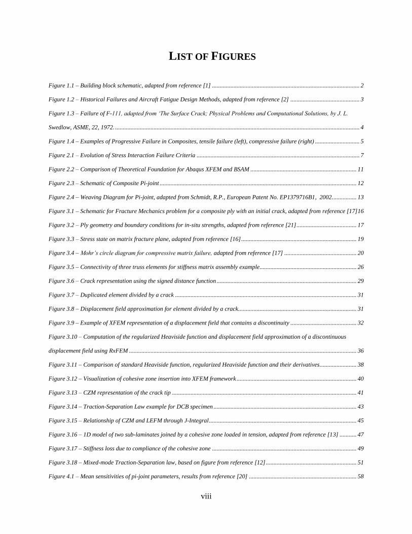
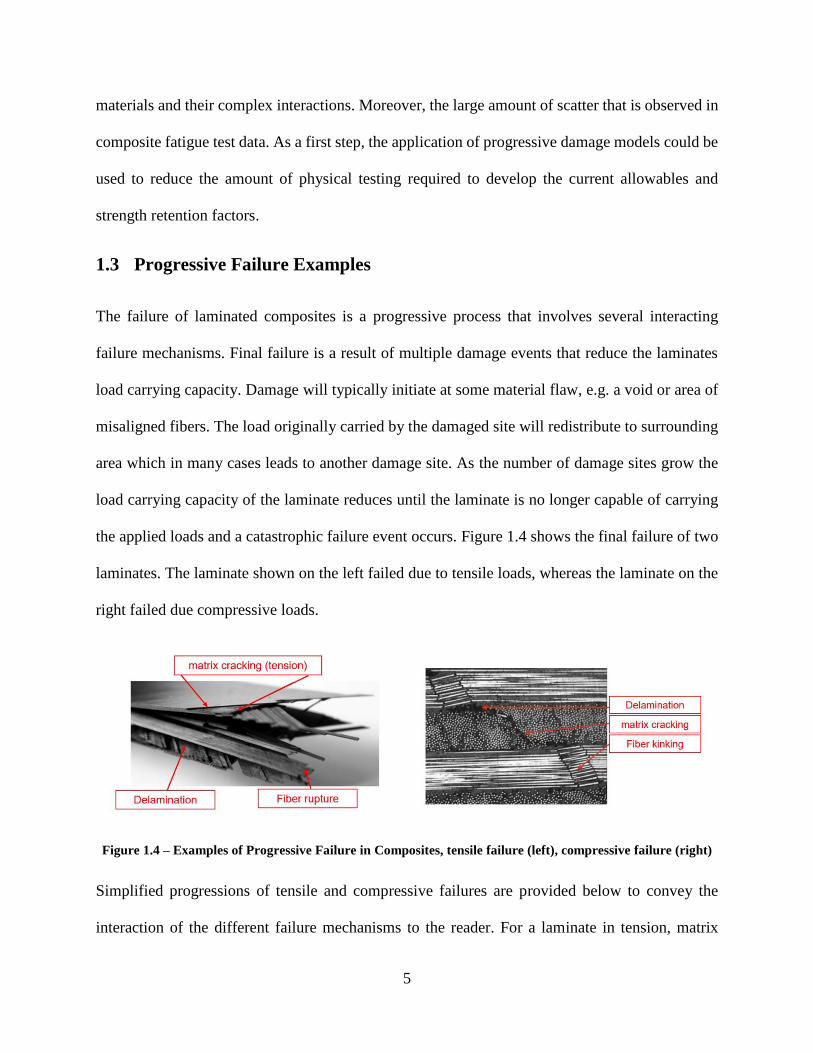
Structural testing and design validation of composite structures in the aerospace industry follow a

building block approach. A depiction of this approach is shown in Figure 1.1 [1].

2

Figure 1.1 – Building block schematic, adapted from reference [1]

At the base of the pyramid is coupon level testing that is used to generate allowables for different

laminate configurations. The allowables generated from the coupon level can be used to design

structural elements at the next level, which then can be used to design structural detail, sub-

components, and eventually components. As the level of the pyramid increases the amount of

testing decreases, i.e. the largest amount of testing will be at the coupon level to determine the

stacking sequences and laminate configurations that will be used in the higher levels. A sizable

amount of the total cost of physical testing for a composite structure is spent at the coupon and

structural element levels. It is at these levels that accurate simulation of progressive damage in

composite materials can be used to provide a cost savings in the development of a composite

structure.

3

1.2 Historical Aerospace Failures and Evolution of Structural Analysis Philosophy

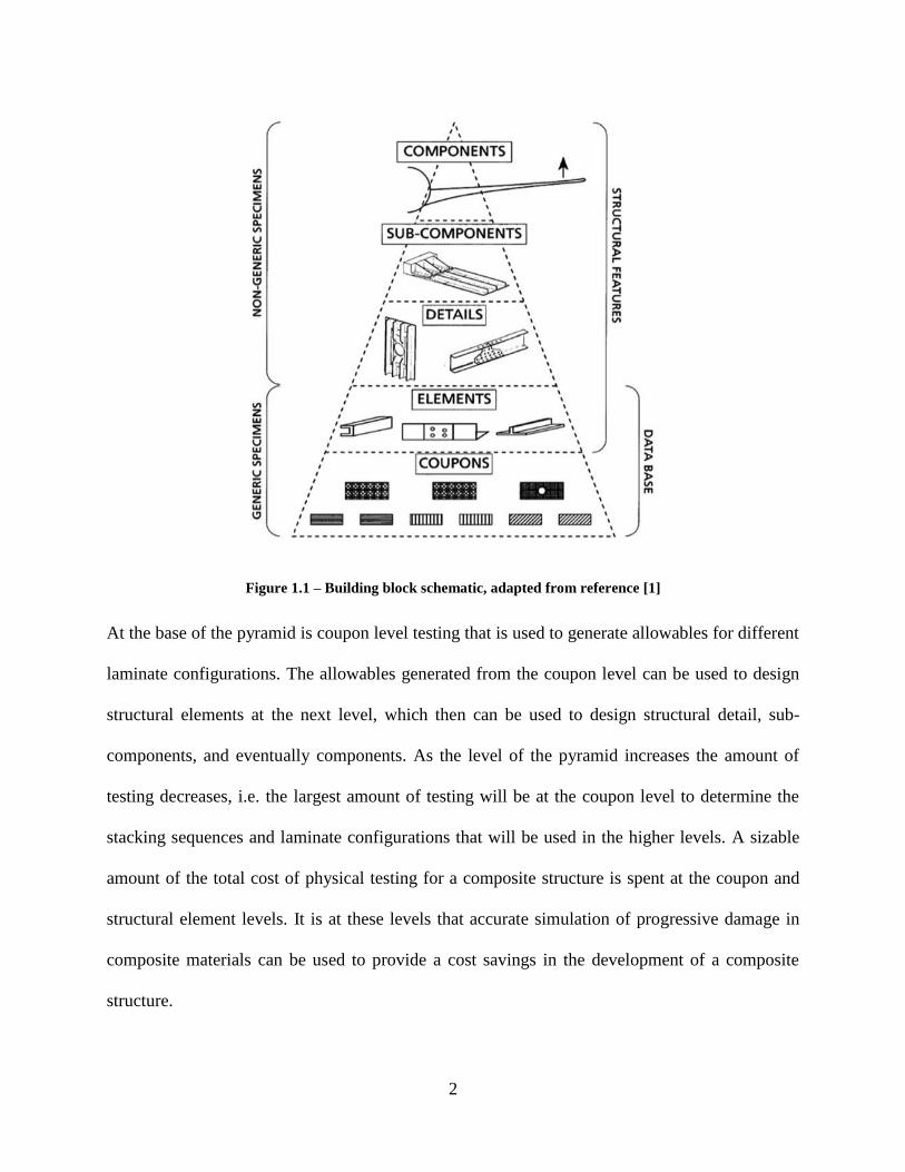
Historical catastrophic failures that resulted in loss of life have shaped the current standards for

designing fatigue resistant aircraft. Figure 1.2 provides a timeline of the different structural

analysis philosophies used to manage fatigue in aircraft since the 1950’s.

Figure 1.2 – Historical Failures and Aircraft Fatigue Design Methods, adapted from reference [2]

Prior to the De Havilland Comet failures in 1954, a Safe-Life approach was used. The Safe-Life

approach used S-N curves to predict fatigue failure and attempted to keep stresses below the

fatigue limit of the material. After the Comet failures in 1954, the Safe-Life approach was deemed

inadequate and the industry adopted the Fail-Safe approach [1]. The Fail-Safe philosophy ensured

that satisfactory fatigue life was achieved without significant cracking and that the structure was

inspectable in service. During this era, the structural requirements were largely met by establishing

redundant load paths that allowed the aircraft to pass residual strength requirements if a single

structural element failed. However, in 1969 a General Dynamics F-111 crashed due to a severed

left wing after only 107 airframe flight hours. Investigations revealed that the wing failed due to

fast fracture after a short period of fatigue growth that initiated from a large manufacturing flaw

[2]. This failure was instrumental in the aerospace industry adopting the Damage Tolerant

approach used today. Damage tolerant design is a fracture mechanics approach that sizes fracture

4

critical parts by assuming that the structure initially contains a flaw of detectable size. Within this

approach the rate at which the initial flaw grows is used to develop the inspection schedule and

ensure that the aircraft can maintain safe flight between inspection intervals.

Figure 1.3 – Failure of F-111, adapted from ‘The Surface Crack; Physical Problems and Computational

Solutions, by J. L. Swedlow, ASME, 22, 1972.

For metallic structure, the failure mechanisms are well understood, and reliable analysis

procedures have been developed to predict fatigue crack growth. Therefore, damage tolerance

requirements can be satisfied by detailed analysis and verifying test data. Conversely, composite

structures satisfy damage tolerant requirements through extensive testing and empirically fitting

test data to generate allowables. The required testing includes residual strength tests after fatigue

and impact damage to develop strength retention factors for various levels of damage that can be

applied in analysis. In other words, the fatigue and damage tolerance requirements are built in to

the static strength allowables through physical testing. While it is unlikely in the near-future,

detailed fracture models of composite materials could one day be used to develop a mechanistic

approach for predicting fatigue crack growth similar to the damage tolerant analysis procedures

for metallic structures. The problem lies with the various failure mechanisms in composite

5

materials and their complex interactions. Moreover, the large amount of scatter that is observed in

composite fatigue test data. As a first step, the application of progressive damage models could be

used to reduce the amount of physical testing required to develop the current allowables and

strength retention factors.

1.3 Progressive Failure Examples

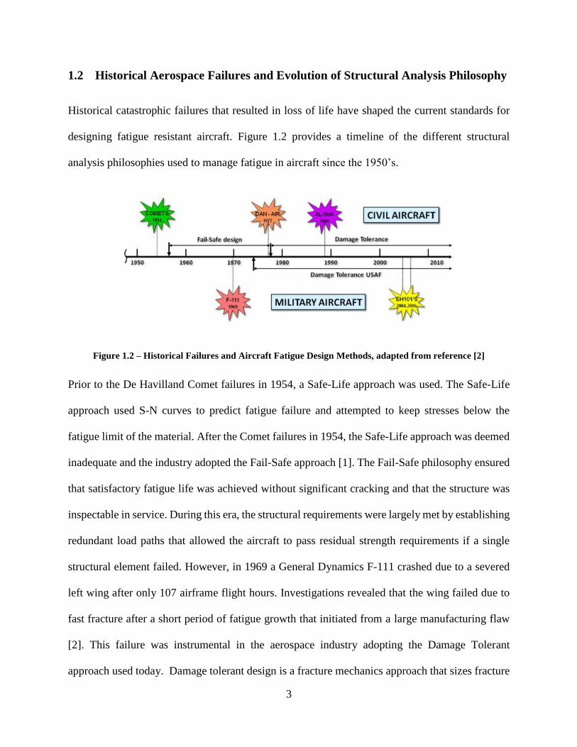
The failure of laminated composites is a progressive process that involves several interacting

failure mechanisms. Final failure is a result of multiple damage events that reduce the laminates

load carrying capacity. Damage will typically initiate at some material flaw, e.g. a void or area of

misaligned fibers. The load originally carried by the damaged site will redistribute to surrounding

area which in many cases leads to another damage site. As the number of damage sites grow the

load carrying capacity of the laminate reduces until the laminate is no longer capable of carrying

the applied loads and a catastrophic failure event occurs. Figure 1.4 shows the final failure of two

laminates. The laminate shown on the left failed due to tensile loads, whereas the laminate on the

right failed due compressive loads.

Figure 1.4 – Examples of Progressive Failure in Composites, tensile failure (left), compressive failure (right)

Simplified progressions of tensile and compressive failures are provided below to convey the

interaction of the different failure mechanisms to the reader. For a laminate in tension, matrix

6

cracking of plies not aligned with the loading direction typically occur first. The number of matrix

cracks grow as the load redistributes in the laminate. Eventually a delamination will initiate from

a matrix crack as a result of localized stress redistribution in the vicinity of the crack. This often

occurs at free edges where the interlaminar stresses are the highest. The delamination will connect

networks of matrix cracks resulting in large redistribution of load throughout the laminate, which

in turn causes more matrix cracks and delaminations to form. At some point, the reduction of load

carrying capacity due to the accumulated damage will reach a critical level. The fibers will no

longer be able to withstand the applied loads and fiber rupture will occur resulting in final laminate

failure.

For a laminate in compression, failure will often occur at locations of fiber misalignment or fiber

waviness. The misalignment of fibers causes an eccentricity of the compressive load and local

fiber bending occurs. This results in a local increase in shear stress at the fiber-matrix interface

and eventually fiber-matrix debonding and matrix cracking. As the fiber-matrix bonds fail, load

redistributes to the neighboring plies which leads to matrix cracking. Delaminations initiate from

the matrix crack networks causing a large redistribution of load and local fiber buckling occurs

resulting in kink-bands at the locations of fiber misalignment and final laminate failure.

It is important to emphasize that the progressive failure descriptions above are purely speculation

and the order of damage events could be different, i.e. matrix cracking could precede the fiber-

matrix debonding in the compressive description. These descriptions are purely intended to

establish the importance of accurately capturing the local effects of damage events as they will

have a large effect on the next predicted event. The more important question becomes how these

failure mechanisms and their interactions are accurately captured using numerical simulation.

7

2. LITERATURE REVIEW

2.1 Development of Failure Criteria

The importance of accounting for stress interaction in predicting failure in composite laminates

has been recognized since the work of Tsai and associates [3] in the late 1960’s and early 1970’s.

The criteria that emerged from these works are known as the Tsai-Hill criterion and Tsai-Wu

criterion. Both criteria use a quadratic approximation and create a smooth failure envelope. Since

a single quadratic expression is used to define the failure envelope, these criteria do not distinguish

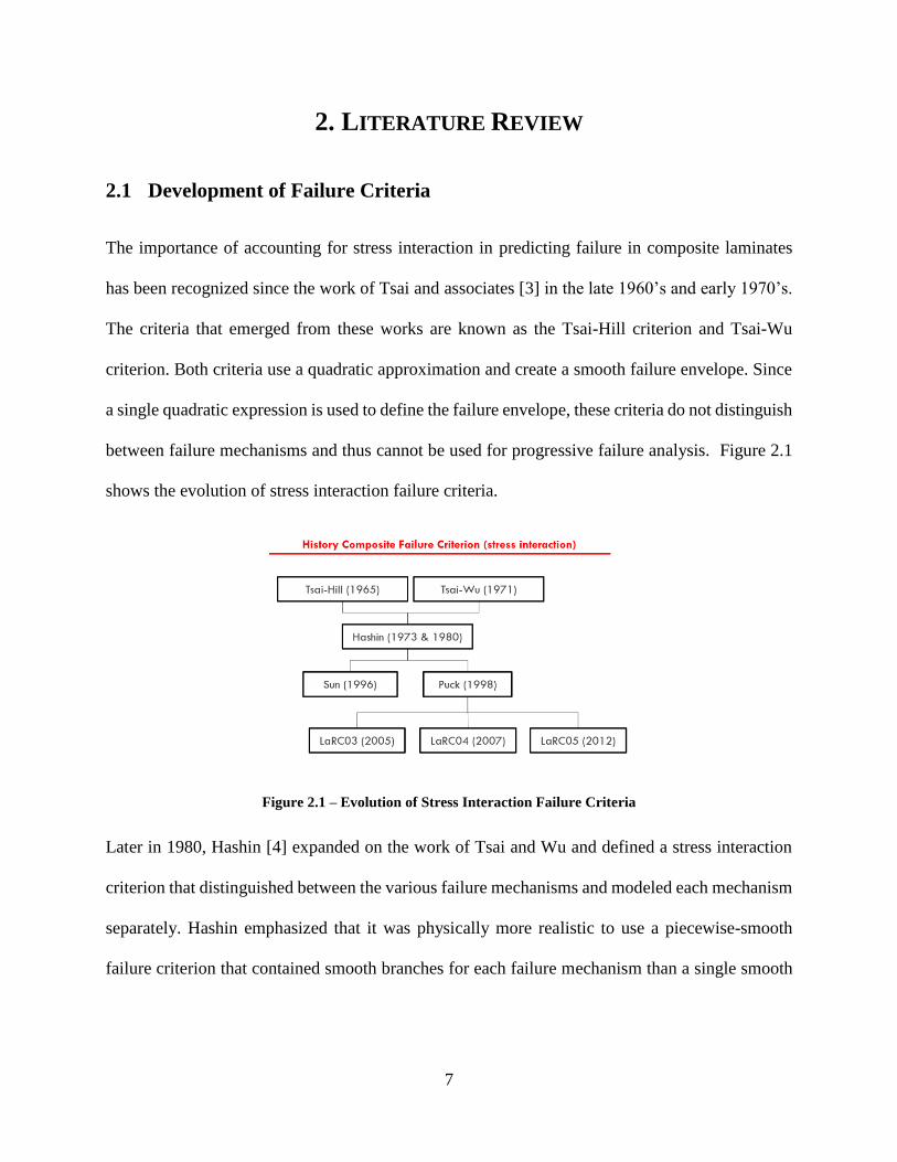
between failure mechanisms and thus cannot be used for progressive failure analysis. Figure 2.1

shows the evolution of stress interaction failure criteria.

Figure 2.1 – Evolution of Stress Interaction Failure Criteria

Later in 1980, Hashin [4] expanded on the work of Tsai and Wu and defined a stress interaction

criterion that distinguished between the various failure mechanisms and modeled each mechanism

separately. Hashin emphasized that it was physically more realistic to use a piecewise-smooth

failure criterion that contained smooth branches for each failure mechanism than a single smooth

8

criterion. Perhaps most importantly, by distinguishing between the different failure mechanisms,

Hashin’s criterion is easily coupled with progressive damage models.

In the early 1990’s, the World Wide Failure Exercise (WWFE) was initiated after a meeting of

subject matter experts on failure in polymeric composites. It was clear after the meeting that there

was a lack of faith in the failure criteria in use at the time and a competition amongst the world’s

experts was initiated to develop a more reliable failure criterion for polymeric composites [5].

Near the conclusion of the WWFE, Puck published his criterion which performed well in the

WWFE. Like Hashin’s criterion, Puck’s criterion was piece-wise smooth and distinguished

between failure mechanisms. It also included effects of shear non-linearity, computation of

fracture plane in compressive matrix failure, and degradation of properties after initial failure [6].

However, as pointed out by Davila in [7] Puck’s criterion incorporated several material parameters

that are not physically based and could be difficult to determine without significant experience

with a given material system.

In the mid 2000’s, at the NASA Langley Research Center (LaRC) a family of failure criteria were

developed by Davila, Pinho and Camanho that were based on the concepts developed by Hashin

and Puck. Like Puck’s criterion, the family of LaRC criteria compute the angle of the fracture

plane for compressive matrix failure, consider kink-band failure mode, and matrix failure in the

misaligned frame. In contrast, all material parameters required for the family of LaRC criteria are

physically based and can be obtained from standard tests [7]. In addition, in-situ strengths are

introduced which establish that matrix strengths are structural properties and account for ply

thickness and boundary conditions. For example, a surface ply of the same material will have a

lower transverse tensile strength than an embedded ply. It is important to note that the LaRC03

criterion is two-dimensional, whereas LaRC04 and LaRC05 are three-dimensional.

9

2.2 Methods of Modeling Damage in Laminated Composites

Continuum Damage Mechanics Approach

Progressive damage of laminated composites has been regularly modeled in the framework of

continuum damage mechanics (CDM). Within the CDM framework, damage is represented by

directionally degrading the volumetric stiffness based on the predicted failure mode. Any

discontinuities in the displacement field due to matrix cracking or fiber damage does not enter the

finite element model. As a result, CDM is easily implemented into conventional non-linear finite

element solvers. In [8], Maimi and Camanho used a CDM approach to model damage

accumulation in an open hole tension specimen with good agreement between numerical

predictions and experimental results. However, a key limitation of this approach is accurately

capturing highly localized interaction of failure modes, i.e. matrix cracking and delamination. [9].

Techniques for Modeling Interface Damage

Delamination has been often modeled using either the virtual crack closure technique (VCCT) or

the cohesive zone model (CZM). VCCT is a fracture mechanics method for predicting

delamination based on the Irwin’s crack closure integral and the assumption that the energy

released by the extension of a crack is equal to the work required to close the crack to its original

length. In [10], Krueger provides a comprehensive summary of the theory and application of

VCCT. In contrast, CZM is a damage mechanics approach for predicting delamination based on

Barentblatt’s theory that there exists a cohesive zone near the crack tip where the upper and lower

faces are held together by a cohesive traction [11]. In the formulation of CZM, the cohesive

tractions are a function of the crack tip opening displacement. At a critical displacement, the

cohesive traction has zero value and the crack propagates. Camanho and Turon have made

10

significant contributions in the development and implementation of cohesive elements into modern

numerical tools. In [12], [13], and [14] the numerical formulation and verification of methods

developed by Camanho and Turon are covered in detail.

Discrete Damage Modeling Approach

In contrast to CDM, in DDM, the kinematics of the displacement jumps due to discontinuities in

the displacement field are directly modeled. In other words, the cracks created due to matrix failure

and delamination are modeled explicitly and the local effects of stress distribution about the cracks

are captured. Delaminations occur at material interfaces where element boundaries exist and

therefore can be implemented into the conventional finite element method as proposed by

Camanho and Turon [14]. However, matrix cracking requires a mesh-independent method that

will allow the cracks to form independent of the mesh orientation. To accomplish this, DDM

methods use the extended finite element method to model matrix cracking independent of the mesh

[15].

Discrete Damage Models in the Current Work

In the current work, two DDM methods were used to predict damage initiation and evolution in a

composite pi-joint test specimen subjected to a pull-off load. These methods will be referred to as

Abaqus XFEM and BSAM. Abaqus XFEM is a commercially available software, whereas BSAM

is research code developed by Iarve and others at the Dayton Research Institute [9], [15] and [25].

DDM methods require three primary components; a failure criterion for predicting damage

initiation, a method for modeling discontinuities in the displacement field, and a constitutive model

for damage accumulation and crack propagation. Figure 2.2 provides a comparison of the

theoretical foundation of the two methods.

11

Figure 2.2 – Comparison of Theoretical Foundation for Abaqus XFEM and BSAM

As shown in Figure 2.2, both Abaqus XFEM and BSAM use failure criteria developed by the

NASA Langley Research Center (LaRC) for crack insertion. Abaqus XFEM uses the LaRC05

criterion [16], whereas BSAM uses the LaRC04 [17] criterion. The two criteria are very similar

with only slight differences on specific failure modes. For more detail on the differences between

LaRC04 and LaRC05 failure criteria refer to Section 3.1. Moreover, both methods use CZM to

model damage accumulation and propagation of matrix cracks and delaminations. Abaqus XFEM

uses a model developed by Camanho and Davila [12], whereas BSAM uses a model developed by

Turon [13]. The formulation of the two CZM models are very similar and will not have a great

effect on the results. The primary theoretical difference between the two methods is the

formulation of the mesh-independent method for modeling matrix cracking. Abaqus XFEM uses

the standard extended finite element formulation [18], whereas BSAM uses a regularized extended

finite element formulation (RxFEM) [15] and [9]. The detail of each formulation is presented latter

in this manuscript. It is important to note that the above comparison is on the theoretical foundation

of the numerical tools and that the numerical engines that run the two methods are vastly different.

12

2.3 Composite Pi-joint Structure

A composite pi-joint is a structural element designed to join spars to skins in aircraft structures.

These joints got their name from utilizing three-dimensional woven preforms that resemble the

Greek letter 𝜋. Figure 2.3 provides a pi-joint configuration for reference. The pi-joint

configuration out performs conventional L-shaped adhesive joints by more evenly redistributing

stress along the bond-line and reducing spikes in peel stress along the preform-skin interface [19].

Figure 2.3 – Schematic of Composite Pi-joint

Moreover, the three-dimensional weaving pattern of the preform provides through-the-thickness

reinforcement and mitigates interlaminar failure modes that commonly occur where the out-of-

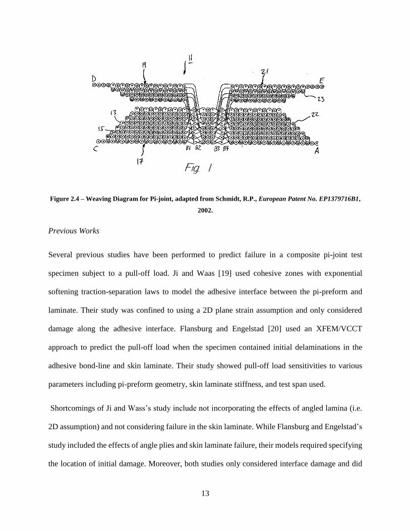
plane stresses are significant. To give the reader an idea of how a pi-preform is constructed, Figure

2.4 provides a schematic of a pi-preform weaving process from a patent filed by Lockheed Martin

Corporation in 2002.

13

Figure 2.4 – Weaving Diagram for Pi-joint, adapted from Schmidt, R.P., European Patent No. EP1379716B1,

2002.

Previous Works

Several previous studies have been performed to predict failure in a composite pi-joint test

specimen subject to a pull-off load. Ji and Waas [19] used cohesive zones with exponential

softening traction-separation laws to model the adhesive interface between the pi-preform and

laminate. Their study was confined to using a 2D plane strain assumption and only considered

damage along the adhesive interface. Flansburg and Engelstad [20] used an XFEM/VCCT

approach to predict the pull-off load when the specimen contained initial delaminations in the

adhesive bond-line and skin laminate. Their study showed pull-off load sensitivities to various

parameters including pi-preform geometry, skin laminate stiffness, and test span used.

Shortcomings of Ji and Wass’s study include not incorporating the effects of angled lamina (i.e.

2D assumption) and not considering failure in the skin laminate. While Flansburg and Engelstad’s

study included the effects of angle plies and skin laminate failure, their models required specifying

the location of initial damage. Moreover, both studies only considered interface damage and did

14

not include the effect of damage within the individual lamina, i.e. matrix cracking and fiber

damage.

Current Study

The current study addresses these shortcomings by using DDM tools that can predict both damage

initiation and evolution in a pristine pi-joint test specimen. Moreover, the DDM tools model both

interlaminar damage (e.g. delamination) and intralaminar damage (e.g. matrix cracking) and their

interaction. To show the effect of ignoring damage within the individual lamina, models that only

accumulate interface damage are included and the results are compared. Using the tool developed

in this work, the location of damage initiation for a given pi-joint configuration can be identified

and flaws can be incorporated at this location to generate durability and damage tolerance

knockdowns.

15

3. THEORETICAL FRAMEWORK

Within this section, the theoretical foundation for the three primary components of discrete damage

modeling are covered in detail. These include a failure criterion for predicting damage initiation,

a method for modeling discontinuities in the displacement field, and a constitutive model for

damage accumulation and crack propagation. For the discrete damage modeling methods used in

this work the following will be covered. First, the LaRC04 and LaRC05 failure criterions will be

presented in the failure criterion section. Next, the traditional finite element method, extended

finite element method, and regularized extended finite element method will be covered in the

section for modeling discontinuities in the displacement field. Finally, the cohesive zone model

will be covered for modeling damage accumulation and crack propagation. Each of these sections

are covered assuming the reader has little knowledge of the subject a priori. Any reader with

detailed knowledge on the subject can use this section purely for reference.

3.1 Damage Initiation Criteria (LaRC Failure Criteria)

For the current work, the LaRC family of failure criteria are used to determine failure locations

and failure mechanisms at the location in question. The LaRC family of failure criteria are based

on the concepts developed by Hashin [4] and Puck [6]. Each criterion in the LaRC family have

different criteria for the following failure modes; matrix tension, matrix compression, matrix

failure in the fiber misalignment frame, fiber tension, and fiber compression. The matrix failure

modes use in-situ strengths in the failure index equations, which account for the ply thickness and

boundary condition of the ply. Note that for the current work, only matrix failure modes were seen

and thus only the formulation of the matrix failure indices will be covered in detail. The reader is

pointed to references [7], [16] and [17] for details on the fiber failure modes.

16

3.1.1 In-situ Strengths

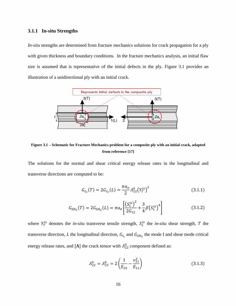
In-situ strengths are determined from fracture mechanics solutions for crack propagation for a ply

with given thickness and boundary conditions. In the fracture mechanics analysis, an initial flaw

size is assumed that is representative of the initial defects in the ply. Figure 3.1 provides an

illustration of a unidirectional ply with an initial crack.

Figure 3.1 – Schematic for Fracture Mechanics problem for a composite ply with an initial crack, adapted

from reference [17]

The solutions for the normal and shear critical energy release rates in the longitudinal and

transverse directions are computed to be:

𝐺𝐼𝐶(𝑇) = 2𝐺𝐼𝐶(𝐿) =𝜋𝑎𝑜2𝛬220 (𝑌𝑇

𝑖𝑠)2 (3.1.1)

𝐺𝑆𝐻C(𝑇) = 2𝐺𝑆𝐻C(𝐿) = 𝜋𝑎0 [(𝑆𝐿

𝑖𝑠)2

2𝐺12+3

4𝛽(𝑆𝐿

𝑖𝑠)4] (3.1.2)

where 𝑌𝑇𝑖𝑠 denotes the in-situ transverse tensile strength, 𝑆𝐿

𝑖𝑠 the in-situ shear strength, 𝑇 the

transverse direction, 𝐿 the longitudinal direction, 𝐺𝐼𝑐 and 𝐺𝑆𝐻C the mode I and shear mode critical

energy release rates, and [𝚲] the crack tensor with 𝛬220 component defined as:

𝛬220 = 𝛬23

0 = 2(1

𝐸22−𝜈212

𝐸11) (3.1.3)

17

These solutions include the effect of shear non-linearity and the reader is pointed to reference [17]

for detail on their derivations. It is important to note that the relation shown in Equation 3.1.4 is

for the special case of the non-linear shear stress-strain relation being approximated by:

𝛾12 =1

𝐺12𝜎12 + 𝛽𝜎12

3 (3.1.5)

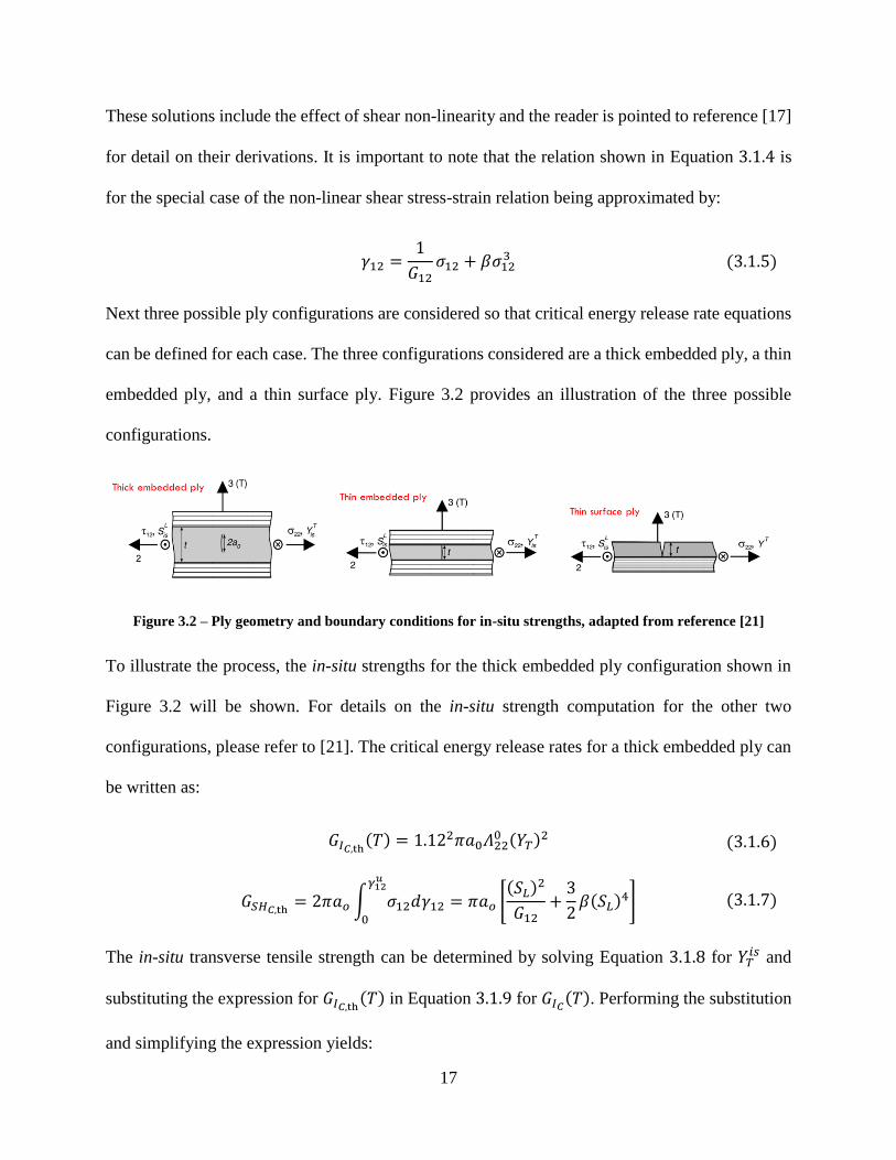
Next three possible ply configurations are considered so that critical energy release rate equations

can be defined for each case. The three configurations considered are a thick embedded ply, a thin

embedded ply, and a thin surface ply. Figure 3.2 provides an illustration of the three possible

configurations.

Figure 3.2 – Ply geometry and boundary conditions for in-situ strengths, adapted from reference [21]

To illustrate the process, the in-situ strengths for the thick embedded ply configuration shown in

Figure 3.2 will be shown. For details on the in-situ strength computation for the other two

configurations, please refer to [21]. The critical energy release rates for a thick embedded ply can

be written as:

𝐺𝐼𝐶,th(𝑇) = 1.122𝜋𝑎0𝛬220 (𝑌𝑇)

2 (3.1.6)

𝐺𝑆𝐻𝐶,th = 2𝜋𝑎𝑜∫ 𝜎12𝑑𝛾12

𝛾12𝑢

0

= 𝜋𝑎𝑜 [(𝑆𝐿)

2

𝐺12+3

2𝛽(𝑆𝐿)

4] (3.1.7)

The in-situ transverse tensile strength can be determined by solving Equation 3.1.8 for 𝑌𝑇𝑖𝑠 and

substituting the expression for 𝐺𝐼𝐶,th(𝑇) in Equation 3.1.9 for 𝐺𝐼𝐶(𝑇). Performing the substitution

and simplifying the expression yields:

18

𝑌𝑇𝑖𝑠 = 1.12√2 𝑌𝑇 (3.1.10)

The computation of the in-situ shear strength is a bit for involved because the resulting expression

has four roots. Performing the same substitution defined above, but using Equations 3.1.11 and

3.1.12 yields the following expression:

(𝑆𝐿

𝑖𝑠)2

2𝐺12+3

4𝛽(𝑆𝐿

𝑖𝑠)4=(𝑆𝐿)

2

𝐺12+3

2𝛽(𝑆𝐿)

4 (3.1.13)

The expression in 3.1.14 has four roots, two imaginary and two real [17]. The in-situ shear strength

𝑆𝐿𝑖𝑠 is the positive real root. A similar process is performed for the other two-ply configuration, but

with different expressions for 3.1.15 and 3.1.16.

3.1.2 LaRC04 Matrix Tension Failure Index

The LaRC04 matrix failure index for transverse tension is based on a mixed-mode fracture

criterion proposed by Hahn [22]. Hahn observed that the fracture surface of specimens that

experienced a higher degree of mode II loading contained more resin hackles. From this

observation, Hahn concluded that more energy is absorbed when larger amounts of mode II loading

are present. As a result, Hahn proposed a criterion for matrix cracking under tension that was

written in terms of the mode I and mode II energy release rates and critical energy release rates as:

(1 − 𝑔)√𝐺𝐼(𝑖)

𝐺𝐼𝐶(𝑖)+ 𝑔

𝐺𝐼(𝑖)

𝐺𝐼𝐶(𝑖)+𝐺𝑆𝐻(𝑖)

𝐺𝑆𝐻𝐶(𝑖)≤ 1, 𝑖 = 𝑇, 𝐿 (3.1.17)

where 𝑔 is the ratio of mode I to mode II critical energy release rates:

𝑔 =𝐺𝐼𝐶𝐺𝑆𝐻𝐶

=𝛬220 (𝑌𝑇

𝑖𝑠)2

𝜒(𝛾12𝑢,𝑖𝑠)

(3.1.18)

19

Substituting in the relations for energy release rates derived in the previous section yields the

LaRC04 failure index for matrix failure under transverse tension.

𝐹𝐼𝑀𝑇= (1 − 𝑔)

𝜎22

𝑌𝑇𝑖𝑠+ 𝑔(

𝜎22

𝑌𝑇𝑖𝑠)

2

+𝛬230 𝜏23

2 + 𝜒(𝛾12𝑢,𝑖𝑠)

𝜒(𝛾12)≤ 1 (3.1.19)

Note that by setting the ratio 𝑔 = 1, ignoring shear non-linearity, and reducing the formulation to

two-dimensions yields the well known-Hashin criterion for matrix failure under transverse tension.

𝐹𝐼𝑀𝑇= (

𝜎22𝑌𝑇)2

+ (𝜏12𝑆𝐿)2

≤ 1 (3.1.20)

3.1.3 LaRC04 Matrix Compression Failure Index

The LaRC04 matrix failure index for transverse compression is assumed to be due to shear stresses

acting on some plane rotated by angle 𝛼 from the plane normal to the loading direction. For pure

compression, many would assume that 𝛼 would be on the plane of maximum shear, i.e. 𝛼 = 45°.

However, it has been experimentally observed by Puck [6] that the fracture occurs on a plane

inclined slightly greater with 𝛼 = 53° ± 2°. The increase in fracture plane under pure compression

is attributed to some amount of friction on the fracture plane. The associated friction is assumed

to decrease as the angle of the fracture plane increases. Therefore, the final fracture occurs on a

plane with 𝛼 > 45°. Figure 3.3 shows the stresses acting on the fracture plane.

Figure 3.3 – Stress state on matrix fracture plane, adapted from reference [16]

20

The stress components acting on the fracture plane can be written in terms of the global ply stresses

using transformation equations as:

𝜎𝑁 =𝜎2 + 𝜎32

+𝜎2 − 𝜎32

𝑐𝑜𝑠(2𝛼) + 𝜏23 𝑠𝑖𝑛(2𝛼) (3.1.21)

𝜏𝑇 = −𝜎2 − 𝜎32

sin(2𝛼) + 𝜏23 cos(2𝛼) (3.1.22)

𝜏𝐿 = 𝜏21 cos(𝛼) + 𝜏31 sin(𝛼) (3.1.23)

The LaRC04 failure index is for matrix compression is then written in terms of the of the stresses

acting on the fracture plane.

𝐹𝐼𝑀c = (𝜏𝑇

𝑆𝑇 − 휂𝑇𝜎𝑁)2

+ (𝜏𝐿

𝑆𝐿𝑖𝑠 − 휂𝐿𝜎𝑁

)

2

≤ 1 (3.1.24)

The fracture plane 𝛼 ∈ [−𝜋, 𝜋] is computed numerically by maximizing the failure index in

Equation 3.1.25. The transverse shear strength 𝑆𝑇 and transverse friction coefficient 휂𝑇 can be

determined geometrically from the Mohr’s circle diagram of the pure compression case shown in

Figure 3.4.

Figure 3.4 – Mohr’s circle diagram for compressive matrix failure, adapted from reference [17]

Using the Mohr’s circle diagram in Figure 3.4, the transverse shear strength is determined by

drawing a line tangent to the Mohr’s circle at an angle of 2𝛼𝑜 from the shear stress axis. The point

at which the tangent line crosses the shear axis is the transverse shear strength. Moreover, the

21

transverse friction factor is the slope of the tangent line. Note that 𝛼𝑜 is the fracture plane under

pure compression and 𝑌𝐶 is the transverse compressive strength, and both are determined

experimentally. These parameters can be written explicitly as:

휂𝑇 = −1

2 tan(2𝛼𝑜) (3.1.26)

𝑆𝑇 = 𝑌𝐶 cos(𝛼𝑜) (sin(𝛼𝑜) +cos(𝛼𝑜)

tan(2𝛼𝑜)) (3.1.27)

The final unknown parameter is the longitudinal friction factor 휂𝐿 and is determined

experimentally. However, Puck [6] suggested in the absence of experimental data the following

relation can be used.

휂𝐿𝑆𝐿=휂𝑇𝑆𝑇

(3.1.28)

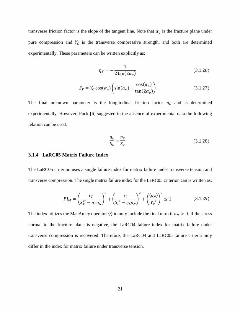
3.1.4 LaRC05 Matrix Failure Index

The LaRC05 criterion uses a single failure index for matrix failure under transverse tension and

transverse compression. The single matrix failure index for the LaRC05 criterion can is written as:

𝐹𝐼𝑀 = (𝜏𝑇

𝑆𝑇𝑖𝑠 − 휂𝑇𝜎𝑁

)

2

+ (𝜏𝐿

𝑆𝐿𝑖𝑠 − 휂𝐿𝜎𝑁

)

2

+ (⟨𝜎𝑁⟩

𝑌𝑇𝑖𝑠)

2

≤ 1 (3.1.29)

The index utilizes the MacAuley operator ⟨∙⟩ to only include the final term if 𝜎𝑁 > 0. If the stress

normal to the fracture plane is negative, the LaRC04 failure index for matrix failure under

transverse compression is recovered. Therefore, the LaRC04 and LaRC05 failure criteria only

differ in the index for matrix failure under transverse tension.

22

3.2 Modeling Discontinuities in the Displacement Field (XFEM/RxFEM)

3.2.1 Finite Element Method

The finite element method is a numerical solution technique for solving complex systems and

geometries for desired field quantities. [23] For this work, the focus will be on the application of

the finite element method in solving structural problems. For a structural problem, it is desired to

acquire the displacement field for a given geometry and set of boundary conditions. To do this, the

continuous geometry is discretized into a discrete domain and the displacements are solved for at

a finite number of points or nodes in the geometry. The nodes are connected by elements which

define the spatial variation and interaction of field quantities between nodes. Using the nodal

displacements and a simple interpolation scheme the displacement at any point in the discretized

domain can be approximated. The stress and strain fields can then be computed from the

approximated displacements.

Isoparametric Formulation

The element formulation implemented in commercial software uses an isoparametric formulation

where the element geometry and displacement field are computed using the same set of

approximation functions, or shape functions. To do this, a reference coordinate system, (𝜉, 휂, 휁),

is used to map a physical element that may be skewed or distorted to a reference element that is a

perfect cube. The equations for the global position and displacements fields as functions of the

reference coordinate system can be written as:

𝑥(𝜉, 휂, 휁) =∑𝑁𝑖(𝜉, 휂, 휁)𝑥𝑖

𝑛

𝑖=1

(3.2.1)

23

𝑢(𝜉, 휂, 휁) =∑𝑁𝑖(𝜉, 휂, 휁)𝑢𝑖

𝑛

𝑖=1

(3.2.2)

where 𝑥𝑖 are the nodal coordinates, 𝑢𝑖 are the nodal displacements, and 𝑁𝑖 are the shape functions.

To obtain the strain field, the displacement field is differentiated with respect to the global

coordinates. However, with the change of coordinates, this is not readily done and the chain rule

must be implemented. This point is illustrated for a simple one-dimensional case below.

휀(𝜉) =𝑑𝑢(𝜉)

𝑑𝑥=𝑑𝜉

𝑑𝑥

𝑑

𝑑𝜉𝑢(𝜉) (3.2.3)

In Equation 3.2.4, the differentiation of the reference coordinate, 𝜉, with respect to the global

coordinate, 𝑥, is not immediately available, however its inverse is. This parameter is the relative

change in distance between coordinate systems or scale factor known as the Jacobian, 𝐽.

𝐽 =𝑑𝑥(𝜉)

𝑑𝜉=∑𝑁𝑖,𝜉(𝜉)𝑥𝑖

𝑛

𝑖=1

(3.2.5)

It is important to note that for two or three-dimensional space, the chain rule will result in a system

of equations and the Jacobian will become a Jacobian matrix. To obtain the strain field, the

expression for the Jacobian is substituted into:.

휀(𝜉) =1

𝐽∑𝑁𝑖,𝜉(𝜉)𝑢𝑖

𝑛

𝑖=1

= [𝐁]{𝐝} (3.2.6)

where

{𝐝} = {𝑢1, 𝑢2…𝑢𝑖 …𝑢𝑛−1, 𝑢𝑛}𝑇 (3.2.7)

and [𝐁] is the strain-displacement matrix. With the strain field obtained, the stress field can be

computed using the appropriate constitutive matrix, [𝐃].

24

𝜎(𝜉) = [𝐃]휀(𝜉) = [𝐃][𝐁]{𝐝} (3.2.8)

Element Stiffness Matrix

Computation of the displacement field, strain field, and stress field have all stemmed from

knowing the nodal displacement vector, {𝐝}. To solve for the nodal displacement vector, the global

stiffness matrix for the discretized structure must be assembled, inverted, and multiplied by the

nodal force vector. The global stiffness matrix is assembled from the individual element stiffness

matrices and the element connectivity. Therefore, the element stiffness matrices must be computed

first. The derivation of the element stiffness matrices can be performed by using the principle of

virtual work. [23]. Mathematically, the principle of virtual work is written as:

∫ {𝛿𝜺}𝑇{𝝈}𝑑ΩΩ

= ∫ {𝛿𝒖}𝑇{𝚽}𝑑𝛤𝛤𝐹

+∫ {𝛿𝒖}𝑇{𝐅}𝑑ΩΩ

(3.2.9)

where {𝚽} represents the surface tractions and {𝐅} the body forces. Note that the symbol 𝛿 has the

same properties as the differential operator, 𝑑. The relations for the stress and strain fields in

Equations 3.2.10 and 3.2.11 can be substituted into 3.2.12 to obtain:

∫ {𝛿𝒅}𝑇[𝐁]𝑇[𝐃][𝐁]{𝐝}𝑑ΩΩ

= ∫ [𝐍]𝑇{𝛿𝒅}𝑇{𝚽}𝑑𝛤𝛤𝐹

+∫ [𝐍]𝑇{𝛿𝒅}𝑇{𝐅}𝑑ΩΩ

(3.2.13)

Note that {𝛿𝒅}𝑇 and {𝐝} can be removed from the integrals because they are not functions of the

coordinates. Doing this and dividing through by {𝛿𝒅}𝑇 yields:

[𝐊𝑒]{𝐝} = {𝐫𝑒} (3.2.14)

where [𝐊𝑒] is the element stiffness matrix, {𝐫𝑒} is the force vector applied to the nodes by the

element, and {𝐝} is the nodal displacements for a given element defined in Equation 3.2.15. Note

that terms for initial stress and strain has been omitted in {𝐫𝑒}.

25

[𝐊𝑒] = ∫ [𝐁]𝑇[𝐃][𝐁]𝑑ΩΩ

(3.2.16)

{𝐫𝑒} = ∫ [𝐍]𝑇{𝚽}𝑑𝛤𝛤𝐹

+∫ [𝐍]𝑇{𝐅}𝑑ΩΩ

(3.2.17)

Evaluating Equation 3.2.18, 𝐽 is a function of 𝜉, therefore the strain-displacement matrix, [𝐁],

contains terms that are rational functions of 𝜉 which cannot be analytically integrated. As a result,

numerical integration techniques are employed to carry out the integration for the element stiffness

matrix. The most commonly used numerical integration scheme is Gauss quadrature because it

provides the highest level of accuracy for a given number of sampling points [23]. The element

stiffness matrix for the one-dimensional case can be approximated numerically as:

[𝐊𝑒] = ∫ [𝐁]𝑇[𝐃][𝐁]1

−1

𝐽 𝑑𝜉 =∑([𝐁]𝑇[𝐃][𝐁] 𝐽)𝜉𝑖𝑊𝑖

𝑛int

𝑖

(3.2.19)

where 𝑛int denotes the number of integration points the integrand is evaluated at, 𝜉𝑖 are the location

of the Gauss or integration points, and 𝑊𝑖 are the corresponding weight factors. This is the standard

process for generating element stiffness matrices for every element in the finite domain. Note that

the stiffness matrix is a function of the nodal geometry (i.e. quad, tri, ect.), shape functions (i.e.

linear or second order), and numerical integration scheme (i.e. full, reduced, ect.) selected. The

different combinations of these parameters make up the vast element library available in

commercial finite element suites.

Assembly of the Global Stiffness Matrix

Using Equation 3.2.20, the element stiffness matrix for all elements in the finite domain can be

computed and the global stiffness matrix can be assembled. The assembly process is straight

26

forward and is based on the fact that elements with shared nodes will mutually influence one

another. For example, consider the assembly of three truss elements shown in Figure 3.5.

Figure 3.5 – Connectivity of three truss elements for stiffness matrix assembly example

The individual element stiffness matrices can be written as:

[𝐊𝑒𝑖 ] = [

𝑘𝑖 −𝑘𝑖

−𝑘𝑖 𝑘𝑖] (3.2.21)

and the global stiffness matrix as:

[𝐊𝐆] =

[ 𝑘1 −𝑘1 0 0

−𝑘1 𝑘1 + 𝑘2 −𝑘2 0

0 −𝑘2 𝑘2 + 𝑘3 −𝑘3

0 0 −𝑘3 𝑘3 ]

(3.2.22)

Comparing Figure 3.5 and the global stiffness matrix, the first node is only affected by the first

spring stiffness. Therefore, only the first spring stiffness contributes to the first entry in the global

stiffness matrix. Similarly, for the fourth node, where only the third spring stiffness contributes.

However, for the second node, both the first and second spring contribute, and the entry in the

global stiffness matrix reflects this by being the sum of the two spring stiffness’s. The same

concept is used to construct global stiffness matrices for complex structures.

27

Computation of the Nodal Displacement Vector

Finally, the nodal displacement vector, {𝐔}, can be obtained using the global stiffness matrix and

nodal force vector, {𝐑}. The fundamental force-displacement relation used in the finite element

method is written as:

[𝐊𝐆]{𝐔} = {𝐑} (3.2.23)

or

{𝐔} = [𝐊𝐆]−𝟏{𝐑} (3.2.24)

With the nodal displacement vector obtained, the displacement field, stress field, and strain field

can all be computed as shown in Equations 3.2.25, 3.2.26, and 3.2.27, respectively.

Key Points

The global stiffness matrix for a finite element domain contains several properties that make the

finite element method robust and scalable for solving large problems. The most critical being

symmetry, sparsity, and that it is singular. The fact that the global stiffness matrix is both

symmetric and sparse allows for highly efficient algorithms to be used when inverting the matrix.

Inverting the global stiffness matrix is an essential step for solving problems with the finite element

method and is typically the most time intensive process. The symmetric and sparse properties allow

this to be done in a fraction of the time it would take to invert a matrix without these properties. In

addition, the global stiffness matrix is singular until boundary conditions that restrain rigid body

motion are applied. This property will make the stiffness matrix un-invertible until proper

boundary conditions are applied providing a check for the user.

In summary, the finite element method provides a simple formulation that can solve problems in

highly complex engineering systems. However, introducing discontinuities to the finite element

28

domain is problematic. A fundamental requirement for convergence in the finite element

formulation is that inter-element continuity is satisfied, meaning that the displacement field cannot

be discontinuous at any point within an element. This makes the modeling of cracks only possible

through element boundaries, which means that the original mesh must be created considering the

location of the crack and re-meshing must be performed as the crack grows. Specifying the location

of an initial crack defeats the purpose of predictive damage modeling, and re-meshing is both time

consuming and has influence on the crack growth.

3.2.2 eXtended Finite Element Method (Abaqus XFEM)

As described in the previous section, introduction of discontinuities into a discretized finite

element domain is not easily handled using the traditional finite element method. Such

discontinuities are limited to element boundaries as the formulation requires inter-element

continuity to obtain a converged solution. To remedy this shortcoming, the eXtended finite element

method (XFEM) was developed. Discontinuities in the finite element domain are essential for

crack growth and will be present in modeling both delamination and matrix cracking in this work.

While delamination can be easily modeled along element boundaries, accurate simulation of

matrix cracking requires a mesh independent method for crack growth.

XFEM Mathematical Formulation

Several XFEM formulations have been proposed for modeling cracks, but the emphasis will be on

the formulation developed by Hansbo and Hansbo [18] that is the basis of the method used in this

work. For a general overview of the different formulations, the reader is pointed to reference [24],

where Belytschko performed a survey on XFEM applications for material modeling. The partition

29

of unity concept of enriching a local domain by adding additional degrees of freedom is common

to all approaches.

In Hansbo and Hansbo’s formulation, discontinuities in a displacement field are handled by

duplicating the original domain and formulating the discontinuous displacement field as a linear

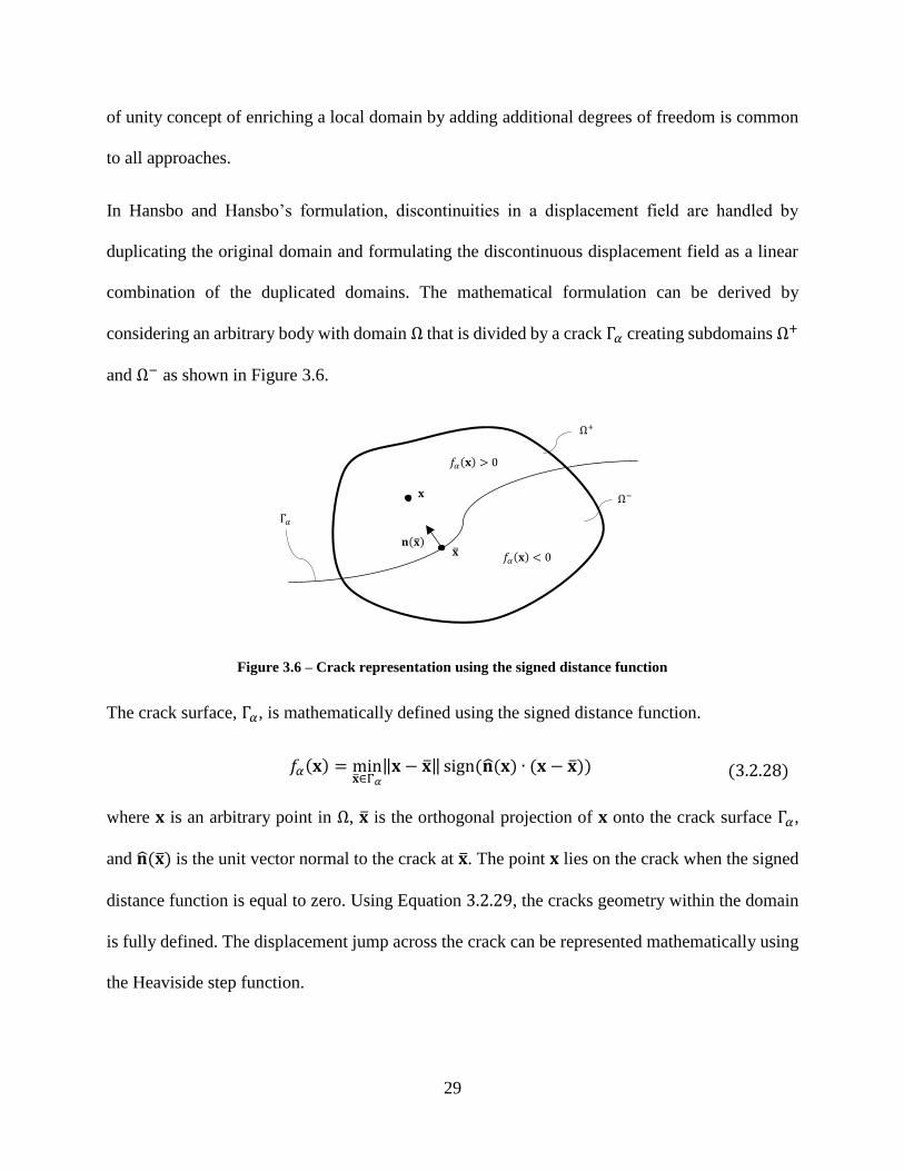
combination of the duplicated domains. The mathematical formulation can be derived by

considering an arbitrary body with domain Ω that is divided by a crack Γ𝛼 creating subdomains Ω+

and Ω− as shown in Figure 3.6.

Figure 3.6 – Crack representation using the signed distance function

The crack surface, Γ𝛼, is mathematically defined using the signed distance function.

𝑓𝛼(𝐱) = min�̅�∈Γ𝛼

‖𝐱 − �̅�‖ sign(�̂�(𝐱) ∙ (𝐱 − �̅�)) (3.2.28)

where 𝐱 is an arbitrary point in Ω, �̅� is the orthogonal projection of 𝐱 onto the crack surface Γ𝛼,

and �̂�(�̅�) is the unit vector normal to the crack at �̅�. The point 𝐱 lies on the crack when the signed

distance function is equal to zero. Using Equation 3.2.29, the cracks geometry within the domain

is fully defined. The displacement jump across the crack can be represented mathematically using

the Heaviside step function.

𝐱

�̅� 𝐧(�̅�)

𝑓𝛼(𝐱) > 0

𝑓𝛼(𝐱) < 0

Γ𝛼

Ω+

Ω−

30

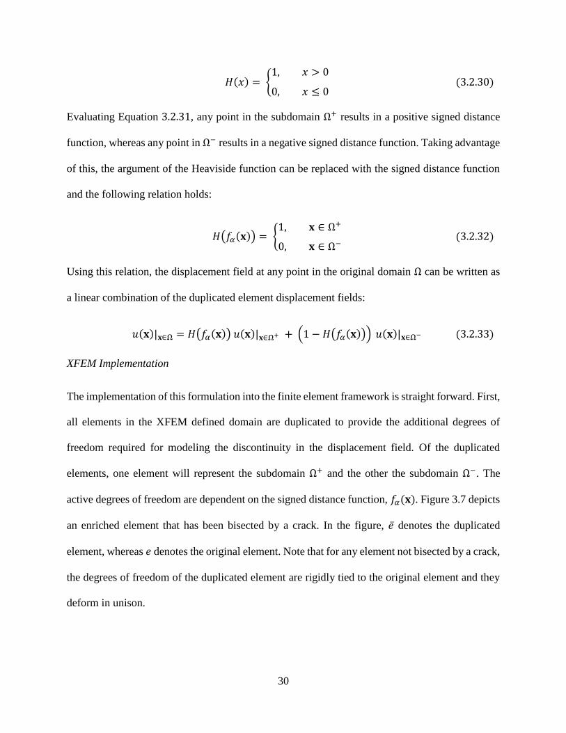
𝐻(𝑥) = {1, 𝑥 > 0

0, 𝑥 ≤ 0 (3.2.30)

Evaluating Equation 3.2.31, any point in the subdomain Ω+ results in a positive signed distance

function, whereas any point in Ω− results in a negative signed distance function. Taking advantage

of this, the argument of the Heaviside function can be replaced with the signed distance function

and the following relation holds:

𝐻(𝑓𝛼(𝐱)) = {1, 𝐱 ∈ Ω+

0, 𝐱 ∈ Ω− (3.2.32)

Using this relation, the displacement field at any point in the original domain Ω can be written as

a linear combination of the duplicated element displacement fields:

𝑢(𝐱)|𝐱∈Ω = 𝐻(𝑓𝛼(𝐱)) 𝑢(𝐱)|𝐱∈Ω+ + (1 − 𝐻(𝑓𝛼(𝐱))) 𝑢(𝐱)|𝐱∈Ω− (3.2.33)

XFEM Implementation

The implementation of this formulation into the finite element framework is straight forward. First,

all elements in the XFEM defined domain are duplicated to provide the additional degrees of

freedom required for modeling the discontinuity in the displacement field. Of the duplicated

elements, one element will represent the subdomain Ω+ and the other the subdomain Ω−. The

active degrees of freedom are dependent on the signed distance function, 𝑓𝛼(𝐱). Figure 3.7 depicts

an enriched element that has been bisected by a crack. In the figure, �̅� denotes the duplicated

element, whereas 𝑒 denotes the original element. Note that for any element not bisected by a crack,

the degrees of freedom of the duplicated element are rigidly tied to the original element and they

deform in unison.

31

Figure 3.7 – Duplicated element divided by a crack

To determine if an element has been split by a crack, the signed distance function is computed for

all nodes in the discretized domain. All nodes that have a positive signed distance function are

assigned to Ω+, whereas nodes with a negative signed distance function are assigned to Ω−. If an

element contains nodes that belong to both subdomains, the element is deemed to be cracked. As

shown in Figure 3.8, let 𝑒 represent the subdomain Ω+ and �̅� the subdomain Ω− [25].

Figure 3.8 – Displacement field approximation for element divided by a crack

The mathematical formulation for the discontinuous displacement field in Equation 3.2.34 is easily

employed into the finite element framework by replacing the displacement fields of elements 𝑒

and �̅� with their finite element approximation, Equation 3.2.35 from Section 3.2.1.

Γ𝛼

Added DOF

Original DOF

Ω𝑒 = Ω�̅�

Twinned

Original Node Non-contributing domain

Contributing domain

Γ𝛼−

Γ𝛼+

�̅� = 𝑒Ω− 𝑒

+ =

32

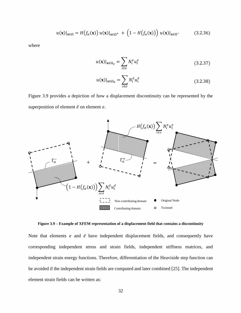
𝑢(𝐱)|𝐱∈Ω = 𝐻(𝑓𝛼(𝐱)) 𝑢(𝐱)|𝐱∈Ω+ + (1 − 𝐻(𝑓𝛼(𝐱))) 𝑢(𝐱)|𝐱∈Ω− (3.2.36)

where

𝑢(𝐱)|𝐱∈Ω𝑒 =∑𝑁𝑖𝑒𝑢𝑖

𝑒

𝑖∈𝑒

(3.2.37)

𝑢(𝐱)|𝐱∈Ω�̅� =∑𝑁𝑖�̅�𝑢𝑖

�̅�

𝑖∈�̅�

(3.2.38)

Figure 3.9 provides a depiction of how a displacement discontinuity can be represented by the

superposition of element �̅� on element 𝑒.

Figure 3.9 – Example of XFEM representation of a displacement field that contains a discontinuity

Note that elements 𝑒 and �̅� have independent displacement fields, and consequently have

corresponding independent stress and strain fields, independent stiffness matrices, and

independent strain energy functions. Therefore, differentiation of the Heaviside step function can

be avoided if the independent strain fields are computed and later combined [25]. The independent

element strain fields can be written as:

+ =

(1 − 𝐻(𝑓𝛼(𝐱)))∑𝑁𝑖�̅�𝑢𝑖

�̅�

𝑖∈�̅�

Γ𝛼− Γ𝛼

+

𝐻(𝑓𝛼(𝐱))∑𝑁𝑖𝑒𝑢𝑖

𝑒

𝑖∈𝑒

Original Node

Twinned Contributing domain

Non-contributing domain

33

휀(𝐱)|𝐱∈Ω𝑒 =∑𝑁𝑖,𝐱𝑒 𝑢𝑖

𝑒

𝑖∈𝑒

= [𝐁]{𝐝𝑒} (3.2.39)

휀(𝐱)|𝐱∈Ω�̅� =∑𝑁𝑖,𝐱�̅� 𝑢𝑖

�̅�

𝑖∈�̅�

= [𝐁]{𝐝�̅�} (3.2.40)

With the independent strain fields, the independent stress fields can be computed using the

appropriate constitutive matrix, [𝐃].

𝜎(𝐱)|𝐱∈Ω𝑒 = [𝐃]휀(𝐱)|𝐱∈Ω𝑒 = [𝐃][𝐁]{𝐝𝑒} (3.2.41)

𝜎(𝐱)|𝐱∈Ω�̅� = [𝐃]휀(𝐱)|𝐱∈Ω�̅� = [𝐃][𝐁]{𝐝�̅�} (3.2.42)

Like the combined displacement field in Equation 3.2.43, the combined stress and strain fields in

the enriched element can be written as:

휀(𝐱)|𝐱∈Ω = 𝐻(𝑓𝛼(𝐱)) 휀(𝐱)|𝐱∈Ω𝑒 + (1 − 𝐻(𝑓𝛼(𝐱))) 휀(𝐱)|𝐱∈Ω�̅� (3.2.44)

𝜎(𝐱)|𝐱∈Ω = 𝐻(𝑓𝛼(𝐱)) 𝜎(𝐱)|𝐱∈Ω𝑒 + (1 − 𝐻(𝑓𝛼(𝐱)))𝜎(𝐱)|𝐱∈Ω�̅� (3.2.45)

Finally, the force-displacement relation for the XFEM element can be obtained by using the

principle of virtual work, Equation 3.2.46, and is expressed as a combination of the independent

stiffness matrices, nodal degrees of freedom, and nodal reaction forces for elements 𝑒 and �̅�.

[𝐊𝑒 𝟎

𝟎 𝐊�̅�] {𝐝𝑒

𝐝�̅�} = {

𝐫𝑒

𝐫�̅�} (3.2.47)

where

[𝐊𝑒] = ∫ [𝐁]𝑇[𝐃][𝐁]𝐻(𝑓𝛼(𝐱))𝑑ΩΩ

(3.2.48)

[𝐊�̅�] = ∫ [𝐁]𝑇[𝐃][𝐁] (1 − 𝐻(𝑓𝛼(𝐱))) 𝑑ΩΩ

(3.2.49)

34

The formulation presented in this section has provided a straight forward extension of the finite

element method to represent element displacement fields that contain discontinuities. However,

the use of the Heaviside function in the formulation has resulted in discontinuous functions in the

integrands of the element stiffness matrices, therefore Gauss quadrature integration defined in

Section 3.2.1 cannot be directly applied [24]. This shortcoming has been remedied by dividing the

original element domain into subdomains with new integration points and performing the

necessary numerical integration only over these subdomains. However, the large number of

possible subdomain configurations and defining the new location of integration points make this

task tedious, time consuming, and not robust. Therefore, it is desirable to develop a formulation

that maintains the elements original integration points so element stiffness matrices can be

computed quickly and consistently.

3.2.3 Regularized eXtended Finite Element Method (BSAM/RxFEM)

As demonstrated in the previous section, XFEM employs the Heaviside step function to introduce

displacement discontinuities across a crack surface. While the introduction of this function allowed

for discontinuities to be modeled within the finite element framework, it also introduced

discontinuous functions into the integrand of the element stiffness matrices. The regularized

extended finite element method provides a solution to this problem by replacing the Heaviside step

function with its continuous approximation. This regularization allows the original element

integration points to be maintained and standard Gauss quadrature integration can be employed.

Heaviside Function Approximation

The regularization of the Heaviside step function was proposed by Iarve [15] where he suggested

that the element shape functions could be used to provide a continuous approximation of the step

35

function. Using the standard Lagrangian shape functions, the step function approximation can be

written as:

�̃�(𝐱) =∑𝑁𝑖(𝐱)ℎ𝑖

𝑛𝑋

𝑖=1

(3.2.50)

where 𝑛𝑋 defines the number of approximation functions and ℎ𝑖 are the Heaviside coefficients

computed by:

ℎ𝑖 =1

2(1 +

∫ 𝑁𝑖(𝐱)𝑓𝛼(𝐱)𝑑𝑉𝑉

∫ 𝑁𝑖(𝐱)|𝑓𝛼(𝐱)|𝑑𝑉𝑉

) (3.2.51)

The coefficients ℎ𝑖 are equal to zero or one if the signed distance function does not change sign in

the nodal support domain, i.e. no member of the nodal support domain is divided by a crack.

Conversely, coefficients ℎ𝑖 will be between zero and one in nodes where any member of its support

domain are divided by a crack [9].

Effects of Heaviside Approximation

The use of the Heaviside approximation does not come without penalty of altering the

mathematical representation of the crack. By using the approximation, the crack surface becomes

a small volume around the crack defined by the region where |∇�̃�(𝐱)| > 0. As a result, the effect

of the crack is distributed across the divided element and its neighbors. To visualize this, a five-

element case is depicted in Figure 3.10.

36

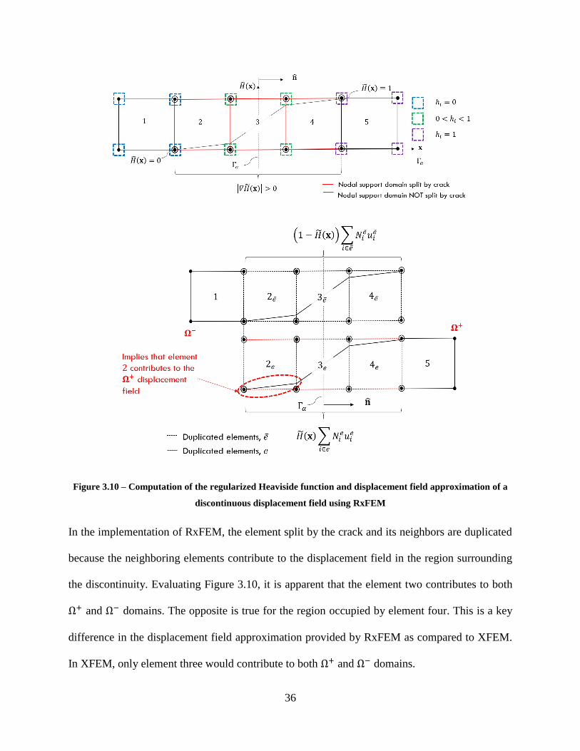
Figure 3.10 – Computation of the regularized Heaviside function and displacement field approximation of a

discontinuous displacement field using RxFEM

In the implementation of RxFEM, the element split by the crack and its neighbors are duplicated

because the neighboring elements contribute to the displacement field in the region surrounding

the discontinuity. Evaluating Figure 3.10, it is apparent that the element two contributes to both

Ω+ and Ω− domains. The opposite is true for the region occupied by element four. This is a key

difference in the displacement field approximation provided by RxFEM as compared to XFEM.

In XFEM, only element three would contribute to both Ω+ and Ω− domains.

37

Distributing the effect of the crack across multiple elements requires justification that considerable

error will not be introduced into the analysis. Evaluating the gradient of the approximated

Heaviside function in Figure 3.11, the size of the zone with non-zero values of ∇𝐻(𝑥) is a function

of element size. This implies that in the limit of mesh refinement the approximated Heaviside

function will approach the true Heaviside function and the magnitude of the approximate gradient

will approach the Dirac delta function. As a result, the gradient of the approximate Heaviside

function will maintain the mathematical properties of the Dirac delta function. Specifically, its

selective property.

∫ 𝛿(𝑥 − 𝑥𝑜)𝑔(𝑥) = 𝑔(𝑥𝑜)∞

−∞

(3.2.52)

This property can be extended to three dimensions and the Dirac delta function can be used to

compute the surface area of the crack.

𝑆𝑣 = ∫ 𝛿𝐷(𝑓𝛼(𝐱))𝑣

𝑑𝑉 ≅ ∫ | ∇�̃�|𝑣

𝑑𝑉 (3.2.53)

This property is key in defining the required fracture energy for crack propagation. A comparison

of an approximated Heaviside function, actual Heaviside function, and their derivatives for a one-

dimensional problem using the standard Lagrangian shape functions is shown in Figure 3.11.

𝐻(𝑥)

𝑥

1

�̃�(𝑥)

𝑥

1

𝑓(𝐿𝑒)

38

Figure 3.11 – Comparison of standard Heaviside function, regularized Heaviside function and their

derivatives

While there is no mathematical proof or derivation that the approximated Heaviside function will

approach the true Heaviside function, Iarve has shown close agreement between RxFEM

approximations and physical test data with sufficient mesh refinement for a number of

configurations [15].

Element Fields and Stiffness Matrix

Accepting agreement of numerical approximation and test data as sufficient proof, the exact

Heaviside step function can be directly replaced with its approximation for the XFEM element

displacement, stress and strain fields as:

𝑢(𝐱)|𝐱∈Ω = �̃�(𝐱) 𝑢(𝐱)|𝐱∈Ω𝑒 + (1 − �̃�(𝐱))𝑢(𝐱)|𝐱∈Ω�̅� (3.2.54)

휀(𝐱)|𝐱∈Ω = �̃�(𝐱) 휀(𝐱)|𝐱∈Ω𝑒 + (1 − �̃�(𝐱)) 휀(𝐱)|𝐱∈Ω�̅� (3.2.55)

𝜎(𝐱)|𝐱∈Ω = �̃�(𝐱) 𝜎(𝐱)|𝐱∈Ω𝑒 + (1 − �̃�(𝐱)) 𝜎(𝐱)|𝐱∈Ω�̅� (3.2.56)

Resulting in the following integrals for the element stiffness matrices:

𝛿(𝑥)

𝑥

∇�̃�(𝑥)

𝑥

𝑓(𝐿𝑒)

39

[𝐊𝑒] = ∫ [𝐁]𝑇[𝐃][𝐁]�̃�(𝐱)𝑑ΩΩ

(3.2.57)

[𝐊�̅�] = ∫ [𝐁]𝑇[𝐃][𝐁] (1 − �̃�(𝐱)) 𝑑ΩΩ

(3.2.58)

The integrands of the stiffness matrices for elements 𝑒 and �̅� are now composed of continuous

functions and the integration domains coincide with the original element domain, therefore the

standard Gauss quadrature method can be employed [25]. For a one-dimensional case the

numerical integration can be written as:

[𝐊𝑒] = ∫ [𝐁]𝑇[𝐃][𝐁]1

−1

�̃�(𝜉𝑖) 𝐽 𝑑𝜉 = ∑([𝐁]𝑇[𝐃][𝐁] 𝐽)𝜉𝑖�̃�(𝜉𝑖)𝑊𝑖

𝑛int

𝑖

(3.2.59)

[𝐊�̅�] = ∫ [𝐁]𝑇[𝐃][𝐁]1

−1

(1 − �̃�(𝜉𝑖)) 𝐽 𝑑𝜉 =∑([𝐁]𝑇[𝐃][𝐁] 𝐽)𝜉𝑖 (1 − �̃�(𝜉𝑖))𝑊𝑖

𝑛int

𝑖

(3.2.60)

Finally, stiffness matrices from Equations 3.2.61 and 3.2.62 can be directly substituted into the

force-displacement relation in Equation 3.2.63.

[ ∫ [𝐁]𝑇[𝐃][𝐁]�̃�(𝐱)𝑑ΩΩ

0

0 ∫ [𝐁]𝑇[𝐃][𝐁] (1 − �̃�(𝐱)) 𝑑ΩΩ ]

{𝐝𝑒

𝐝�̅�} = {

𝐫𝑒

𝐫�̅�} (3.2.64)

Note that the formulation derived in this section is for an element that has been completely divided

by a crack. The complete separation is represented in the element stiffness matrix by the off-

diagonal terms being equal to zero. In other words, the zero valued off diagonal terms physically

represent no interaction between the 𝑒 and �̅� element displacement fields. Conversely, if an

element is in the fracture process zone, a cohesive zone can be directly inserted along the crack

surface or in the case of the RxFEM the gradient zone. If this is done, the zero value off diagonal

terms will become non-zero and will be dependent on the traction-separation law used in the

40

model. In this work, cohesive zone models will be used explicitly to model the crack behavior in

fracture process zones. A detailed overview of the cohesive zone models used in this work are

outlined in Section 3.3. Figure 3.12 gives a visualization of how the cohesive zone is inserted into

the XFEM framework. For RxFEM cohesive traction-separation laws would also be entered into

neighboring elements where |∇�̃�(𝑥)| > 0.

Figure 3.12 – Visualization of cohesive zone insertion into XFEM framework

3.3 Modeling Damage Accumulation and Crack Propagation (CZM)

For the current work, cohesive zone models will be used exclusively to model damage

accumulation in a composite pi-joint. Baseline finite element models with cohesive interfaces will

be compared with Abaqus XFEM and BSAM models that include the effects of matrix cracking

on damage progression. The Abaqus Interface models and Abaqus XFEM models will use the

traditional point-wise crack opening displacements to track interface damage, whereas the BSAM

model will use a fracture energy balance in the gradient zone for both matrix cracks and interface

delamination [9].

Original Node

Twinned Node Contributing domain

Non-contributing domain

Traction-Separation Law

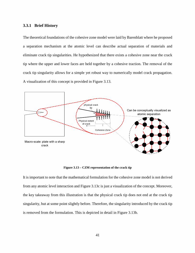
41

3.3.1 Brief History

The theoretical foundations of the cohesive zone model were laid by Barenblatt where he proposed

a separation mechanism at the atomic level can describe actual separation of materials and

eliminate crack tip singularities. He hypothesized that there exists a cohesive zone near the crack

tip where the upper and lower faces are held together by a cohesive traction. The removal of the

crack tip singularity allows for a simple yet robust way to numerically model crack propagation.

A visualization of this concept is provided in Figure 3.13.

Figure 3.13 – CZM representation of the crack tip

It is important to note that the mathematical formulation for the cohesive zone model is not derived

from any atomic level interaction and Figure 3.13c is just a visualization of the concept. Moreover,

the key takeaway from this illustration is that the physical crack tip does not end at the crack tip

singularity, but at some point slightly before. Therefore, the singularity introduced by the crack tip

is removed from the formulation. This is depicted in detail in Figure 3.13b.

42

3.3.2 Traction-Separation Laws

In a cohesive zone model, traction-separation laws are used to define the nodal tractions as a

function of the displacement jumps. A traction-separation law can be thought of as unique spring

behavior, where the spring stiffness is a function of displacement and degrades after a critical

displacement is reached until final failure occurs. In the finite element method, nodal

displacements are readily available, therefore defining interface behavior as a function of

displacement is ideal.

There have been several traction-separation laws proposed over the years with the most popular

being the bi-linear, linear-parabolic, exponential, and trapezoidal. In 2005, Alfano performed a

study in which he compared the accuracy and numerical efficiency of these laws for pure mode

loading [26]. Alfano determined that the shape of the traction-separation law had negligible effect

on the accuracy of the solution away from the peak load. Moreover, the bi-linear law provided the

best combination of accuracy and numerical performance. Figure 3.14 provides a schematic that

shows how points in a bi-linear traction-separation law correlate to the physical state of the

interface.

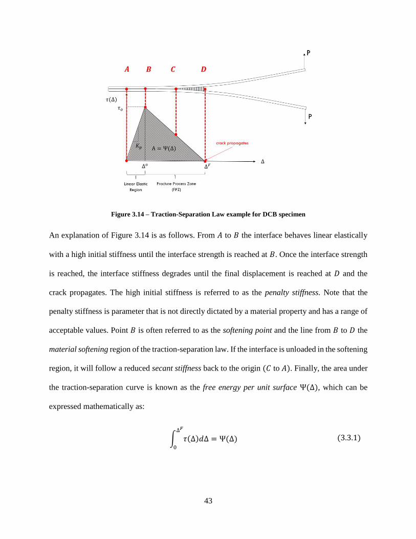
43

Figure 3.14 – Traction-Separation Law example for DCB specimen

An explanation of Figure 3.14 is as follows. From 𝐴 to 𝐵 the interface behaves linear elastically

with a high initial stiffness until the interface strength is reached at 𝐵. Once the interface strength

is reached, the interface stiffness degrades until the final displacement is reached at 𝐷 and the

crack propagates. The high initial stiffness is referred to as the penalty stiffness. Note that the

penalty stiffness is parameter that is not directly dictated by a material property and has a range of

acceptable values. Point 𝐵 is often referred to as the softening point and the line from 𝐵 to 𝐷 the

material softening region of the traction-separation law. If the interface is unloaded in the softening

region, it will follow a reduced secant stiffness back to the origin (𝐶 to 𝐴). Finally, the area under

the traction-separation curve is known as the free energy per unit surface Ψ(∆), which can be

expressed mathematically as:

∫ 𝜏(∆)𝑑∆∆𝐹

0

= Ψ(∆) (3.3.1)

44

For a bi-linear law, Ψ(∆) is simply the area of the triangle with height equal to the interface

strength 𝜏𝑜 and base the maximum displacement ∆𝐹. Using this, the maximum displacement can

be written as:

∆𝐹=2Ψ(∆)

𝜏𝑜 (3.3.2)

To fully define the shape of the bi-linear law, the displacement at the onset of damage ∆𝑜 must be

computed. Knowing the interface behaves linearly elastic up to the interface strength, ∆𝑜 can be

determined from the interface strength and initial or penalty stiffness 𝐾𝑝.

∆𝑜=𝜏𝑜𝐾𝑝

(3.3.3)

While there is no clear definition of what the penalty stiffness should be, it is known that it must

be great enough to ensure a stiff connection between the two neighboring layers, but not so high

that numerical instability becomes an issue [13]. The selection of this parameter has a greater

influence on the numerical stability than the accuracy of the solution. Further detail on penalty

stiffness latter in this section.

In summary, traction-separation laws are used to define interface behavior in cohesive zones.

Having the interface behavior as a function of displacement allows for easy implementation in the

finite element method. A bi-linear law is fully defined with input parameters 𝜏𝑜, Ψ(∆), and 𝐾𝑝.

The materials interface strength and fracture toughness can be used to define 𝜏𝑜 and Ψ(∆),

respectively, whereas 𝐾𝑝 is selected based on a rough set of guidelines. These parameters are input

into Equations 3.3.4 and 3.3.5 to compute critical displacements for damage onset and crack

propagation.

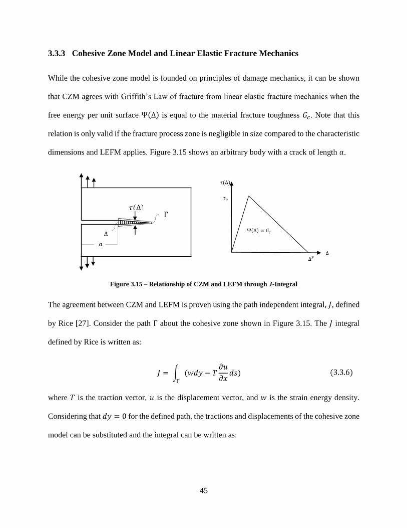
45

3.3.3 Cohesive Zone Model and Linear Elastic Fracture Mechanics

While the cohesive zone model is founded on principles of damage mechanics, it can be shown

that CZM agrees with Griffith’s Law of fracture from linear elastic fracture mechanics when the

free energy per unit surface Ψ(∆) is equal to the material fracture toughness 𝐺𝑐. Note that this

relation is only valid if the fracture process zone is negligible in size compared to the characteristic

dimensions and LEFM applies. Figure 3.15 shows an arbitrary body with a crack of length 𝑎.

Figure 3.15 – Relationship of CZM and LEFM through J-Integral

The agreement between CZM and LEFM is proven using the path independent integral, 𝐽, defined

by Rice [27]. Consider the path Γ about the cohesive zone shown in Figure 3.15. The 𝐽 integral

defined by Rice is written as:

𝐽 = ∫ (𝑤𝑑𝑦 − 𝑇𝜕𝑢

𝜕𝑥𝑑𝑠)

Γ

(3.3.6)

where 𝑇 is the traction vector, 𝑢 is the displacement vector, and 𝑤 is the strain energy density.

Considering that 𝑑𝑦 = 0 for the defined path, the tractions and displacements of the cohesive zone

model can be substituted and the integral can be written as:

𝜏(∆)

∆ ∆𝐹

Ψ(∆) = 𝐺𝑐

𝜏𝑜

Γ 𝜏(∆)

∆

𝑎

46

𝐽 = −∫ 𝜏(∆)𝑑∆

𝑑𝑥𝑑𝑥

Γ

= −∫𝑑

𝑑𝑥(∫ 𝜏(∆)𝑑𝛿

∆𝐹

0

)𝑑𝑥Γ

= ∫ 𝜏(∆)𝑑∆∆𝐹

0

(3.3.7)

Similarly, using Griffith’s theory it has been shown for small scale yielding in LEFM the 𝐽 integral

can be used to define the change in potential energy with respect to the crack length and written as

[28]:

𝐽 = −𝜕Π

𝜕𝑎= 𝐺 (3.3.8)

where Π is the total potential energy, 𝑎 is the crack length, and 𝐺 is the energy release rate. When

𝐽 reaches the critical value before crack propagation the following relation holds.

𝐽 = 𝐺𝑐 = ∫ 𝜏(∆)𝑑∆∆𝐹

0

(3.3.9)

where 𝐺𝑐 is the fracture toughness of the material and ∆𝐹 is the maximum displacement before

crack propagation occurs.

3.3.4 Cohesive Zone Parameters

The selection of parameters that define the constitutive behavior are key to obtaining converged

and accurate solutions when modeling cohesive interfaces. As previously pointed out, the

parameters that fully define the constitutive behavior of the cohesive zone are 𝐾𝑝, 𝜏𝑜 and Ψ(∆).

The value of Ψ(∆) is defined by the interface fracture toughness and altering its value will have a

large effect on the accuracy of the solution. Conversely, 𝐾𝑝 and 𝜏𝑜 have a range of acceptable

values that will provide accurate solutions.

While the interface strength 𝜏𝑜 is a material property, it has been shown by Turon [13] that

changing its value has little effect on the accuracy of the solution if the area under the traction-

separation law remains equivalent to the interface fracture toughness and LEFM applies.

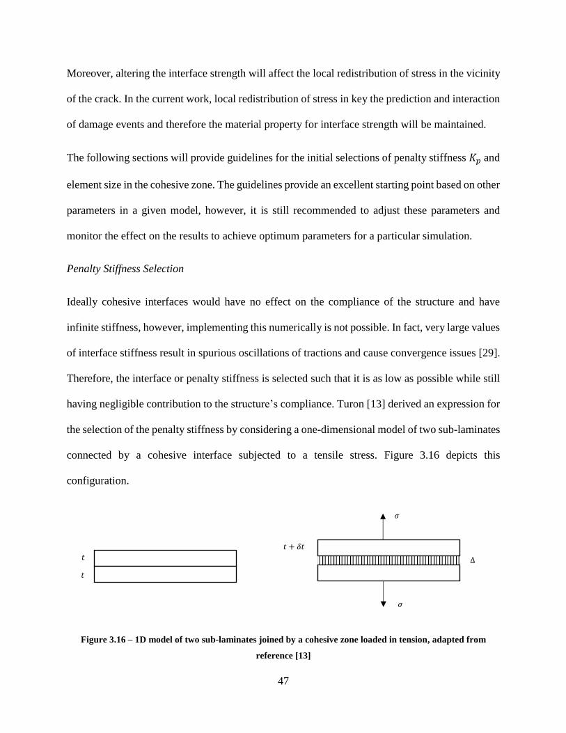
47

Moreover, altering the interface strength will affect the local redistribution of stress in the vicinity

of the crack. In the current work, local redistribution of stress in key the prediction and interaction

of damage events and therefore the material property for interface strength will be maintained.

The following sections will provide guidelines for the initial selections of penalty stiffness 𝐾𝑝 and

element size in the cohesive zone. The guidelines provide an excellent starting point based on other

parameters in a given model, however, it is still recommended to adjust these parameters and

monitor the effect on the results to achieve optimum parameters for a particular simulation.

Penalty Stiffness Selection

Ideally cohesive interfaces would have no effect on the compliance of the structure and have

infinite stiffness, however, implementing this numerically is not possible. In fact, very large values

of interface stiffness result in spurious oscillations of tractions and cause convergence issues [29].

Therefore, the interface or penalty stiffness is selected such that it is as low as possible while still

having negligible contribution to the structure’s compliance. Turon [13] derived an expression for

the selection of the penalty stiffness by considering a one-dimensional model of two sub-laminates

connected by a cohesive interface subjected to a tensile stress. Figure 3.16 depicts this

configuration.

Figure 3.16 – 1D model of two sub-laminates joined by a cohesive zone loaded in tension, adapted from

reference [13]

𝑡

𝑡

𝑡 + 𝛿𝑡

∆

𝜎

𝜎

48

Equilibrium requires that:

𝜎 = 𝐾𝑝∆= 𝐸3휀 = 𝐸eff휀eff (3.3.10)

The effective strain of the sub-laminate and cohesive interface can be written as:

휀eff =𝛿𝑡

𝑡+∆

𝑡= 휀 +

∆

𝑡 (3.3.11)

From the equilibrium equation the sub-laminate strain can be expressed as:

휀 =𝐾𝑝∆

𝐸3 (3.3.12)

Substituting Equation 3.3.13 into 3.3.14 then into 3.3.15 the effective modulus as a function of

the sub-laminate modulus and penalty stiffness becomes:

𝐸eff = 𝐸3(1

1 +𝐸3𝐾𝑝𝑡

) (3.3.16)

Evaluating Equation 3.3.17 the compliance of the sub-laminate is not affected by the cohesive

interface when 𝐾𝑝𝑡 ≫ 𝐸3, which leads to the following expression for the selection of the penalty

stiffness.

𝐾𝑝 =𝛼𝐸3𝑡

(3.3.18)

Figure 3.17 shows a plot of 𝐸eff 𝐸3⁄ as a function of the defined constant 𝛼. When 𝛼 > 50 the

stiffness loss due to the cohesive interface is less than two percent.

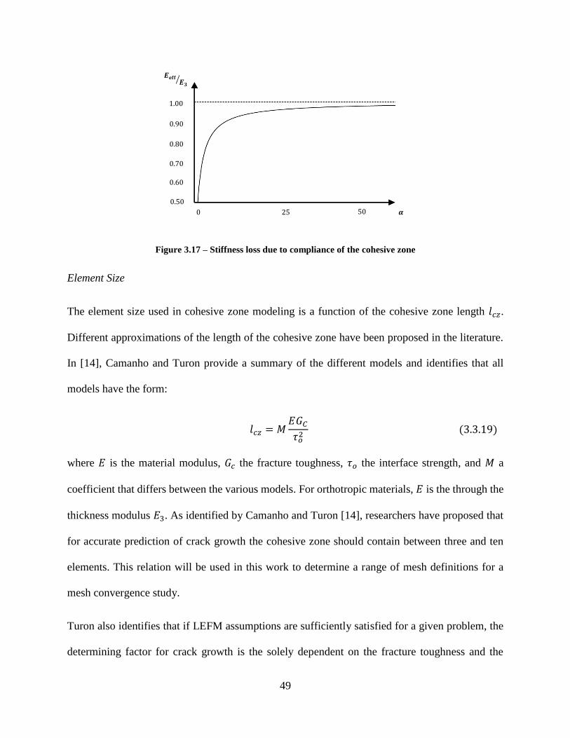
49

Figure 3.17 – Stiffness loss due to compliance of the cohesive zone

Element Size

The element size used in cohesive zone modeling is a function of the cohesive zone length 𝑙𝑐𝑧.

Different approximations of the length of the cohesive zone have been proposed in the literature.

In [14], Camanho and Turon provide a summary of the different models and identifies that all

models have the form:

𝑙𝑐𝑧 = 𝑀𝐸𝐺𝐶𝜏𝑜2

(3.3.19)

where 𝐸 is the material modulus, 𝐺𝑐 the fracture toughness, 𝜏𝑜 the interface strength, and 𝑀 a

coefficient that differs between the various models. For orthotropic materials, 𝐸 is the through the

thickness modulus 𝐸3. As identified by Camanho and Turon [14], researchers have proposed that

for accurate prediction of crack growth the cohesive zone should contain between three and ten

elements. This relation will be used in this work to determine a range of mesh definitions for a

mesh convergence study.

Turon also identifies that if LEFM assumptions are sufficiently satisfied for a given problem, the

determining factor for crack growth is the solely dependent on the fracture toughness and the

𝑬𝐞𝐟𝐟𝑬𝟑ൗ

1.00

0.90

0.80

0.70

0.60

0.50

0 25 50 𝜶

50

interface strength can be adjusted to increase the size of the cohesive zone. In Equation 3.3.20, the

length of the cohesive zone is inversely proportional to the square of the interface strength 𝜏𝑜,

therefore, reducing the interface strength will have a considerable effect on the cohesive zone

length and coarser meshes can be used. However, reducing the interface strength will also alter the

redistribution of stress, which is critical in predicting local damage events and their interactions in

the current work. Therefore, this technique will not be used.

3.3.5 General Case – Mixed-mode Constitutive Model

This section will cover the mixed-mode constitutive model developed by Camanho and Davila

[12] that is used in the Abaqus Interface models and Abaqus XFEM models. The mixed-mode

constitutive behavior developed by Turon [13] that is implemented in the BSAM models is very

similar and will not be repeated. One key difference in the computation of damage onset will be

identified. The reader is pointed to [13] for more details on Turron’s model.

When a delamination occurs in a structure, the interface loading is typically a function of multiple

modes of fracture. Additionally, it is common for the mode-mix to change as delamination

propagates in the structure. Therefore, there is a need for a generalized constitutive behavior that

is valid for any combination of normal and shear loading. The traction-separation law shown in

Section 3.3.2 is for a particular mode-mix, say pure mode I loading. A generalized traction-

separation law valid for any mode-mix is represented in Figure 3.18.

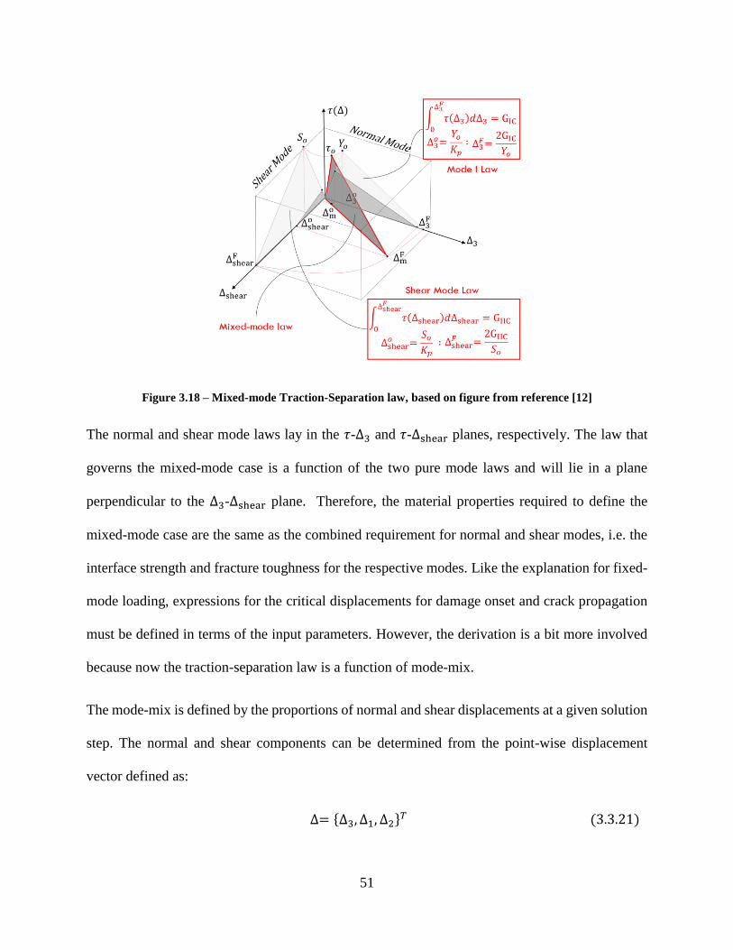
51

Figure 3.18 – Mixed-mode Traction-Separation law, based on figure from reference [12]

The normal and shear mode laws lay in the 𝜏-∆3 and 𝜏-∆shear planes, respectively. The law that

governs the mixed-mode case is a function of the two pure mode laws and will lie in a plane

perpendicular to the ∆3-∆shear plane. Therefore, the material properties required to define the

mixed-mode case are the same as the combined requirement for normal and shear modes, i.e. the

interface strength and fracture toughness for the respective modes. Like the explanation for fixed-

mode loading, expressions for the critical displacements for damage onset and crack propagation

must be defined in terms of the input parameters. However, the derivation is a bit more involved

because now the traction-separation law is a function of mode-mix.

The mode-mix is defined by the proportions of normal and shear displacements at a given solution

step. The normal and shear components can be determined from the point-wise displacement

vector defined as:

∆= {∆3, ∆1, ∆2}𝑇 (3.3.21)

52

where ∆1 and ∆2 are the shear displacement components and ∆3 is the normal displacement

component. Note that in this constitutive model, the fracture mechanism for mode II and mode III

are assumed to be the same and their combined interaction is lumped into a single shear mode.

This allows the kinematic formulation for the interface defined in references [12] and [13] to be

valid. In terms of the local displacements, the shear displacement is defined as the norm of the

mode II and mode III displacement components and can be written as:

∆shear= √∆22 + ∆1

2 (3.3.22)

Note that the assumption made to combine the shear interactions leads to the following relations:

𝑇 = 𝑆 (3.3.23)

∆1𝑜= ∆2

𝑜= ∆shear𝑜 =

𝑆

𝐾𝑝

(3.3.24)

where 𝑆 and 𝑇 are the interface strengths in mode II and mode III, respectively. The mixed-mode

traction-separation law uses a total displacement jump ∆m to determine the points of damage

initiation and crack propagation. The total mixed-mode displacement jump is defined as the norm

of the normal and shear displacement components.

∆m= √∆shear2 + ⟨∆3⟩2 (3.3.25)

where ⟨∙⟩ is the MacAuley operator and is defined as:

⟨𝑥⟩ = {𝑥, 𝑥 > 00, 𝑥 ≤ 0

(3.3.26)

This displacement value will be computed at each solution step and compared against the critical

displacement values. The critical displacement values are points at which damage onset and crack

propagation occur and are defined by a selected failure criteria and propagation criteria,

53

respectively. A number of failure and propagation criteria are available in Abaqus. The following

paragraphs will define the selections used in this work. Note that Equation 3.3.27 is written so that

normal displacements only contribute if the displacement correlates to a tensile or crack opening

load at the interface.

During mixed-mode delamination, damage can initiate before any of the individual interface

strengths are reached. To account for the mode interaction, the damage initiation criteria used in

the Abaqus Interface and Abaqus XFEM models is a quadratic approximation analogous to the

Tsai-Hill criterion for composite laminates. In Abaqus, this failure criteria is referred to as the

quadratic traction criteria.

(⟨𝜏3⟩

𝑁)

2

+ (𝜏2𝑆)2

+ (𝜏1𝑇)2

= 1 (3.3.28)

Using this failure criteria, the total mixed-mode displacement jump at the onset of damage ∆m𝑜 can

be computed. Substituting the mode I, II, and II interface strengths in term of penalty stiffness and

critical displacements into the quadratic traction criteria, ∆m𝑜 can be written as:

∆mo =

{

∆3o∆shear

o√

1 + 𝛽2

(∆ shearo )

2+ (𝛽∆)2

, ∆3> 0

∆shearo , ∆3≤ 0

(3.3.29)

where 𝛽 is the shear-normal mode-mix ratio defined as:

𝛽 =∆shear∆3

, ∆3 > 0 (3.3.30)

A complete derivation of the expression in Equation 3.3.31 is provided in reference [12]. The final

parameter needed to fully define the mixed-mode traction-separation law is the criteria for crack

propagation. For this work, an energy method is used that is based on an equivalent fracture

54

toughness for a given mode-mix. For delamination of composites, the B-K criterion has been

shown to be the most accurate [12]. Benzeggagh and Kenane developed this criterion using a

mixed-mode bending test specimen and empirically fitting the measured equivalent fracture

toughness with a curve that is a function of the two pure mode fracture toughnesses and the energy

mode ratio 𝐵 [31]. This empirical formula is written as:

𝐺𝐶(𝐵) = 𝐺𝐼𝐶 + (𝐺𝐼𝐼𝐶 − 𝐺𝐼𝐶)𝐵𝜂 (3.3.32)

where the energy mode ratio is:

𝐵 =𝐺shear𝐺𝑇

(3.3.33)

and 휂 is the empirical constant determined from a least square curve fit of the experimental data.

The relation between the ratio 𝐵 and 𝛽 is shown to be:

𝐵 =𝛽2

1 + 𝛽2 (3.3.34)

Similar to Section 3.3.2, the critical displacement before crack propagation ∆m𝐹 can be computed

from the equivalent fracture toughness 𝐺𝐶(𝐵) and the displacement at the onset of damage ∆m𝑜 .

∆m𝐹 =

2𝐺𝐶(𝐵)

∆m𝑜 (3.3.35)

Substituting Equation 3.3.36 into 3.3.37 then into 3.3.38 and solving for the critical displacement

for crack propagation yields.

∆m𝐹 = {

2

𝐾𝑝∆m𝑜 [𝐺𝐼𝐶 + (𝐺𝐼𝐼𝐶 − 𝐺𝐼𝐶) (

𝛽2

1 + 𝛽2)

𝜂

] , ∆3> 0

∆shear𝐹 , ∆3≤ 0

(3.3.39)

55

With 𝐾𝑝, 𝐺𝑐(𝐵), ∆m𝑜 , and ∆m

𝐹 the traction-separation law for the mixed-mode case is fully defined

as a function of the local displacements and is valid for any mode-mix ratio. The constitutive

equation for the tractions at any point on the mixed-mode bi-linear law can be written as:

{𝝉} = [𝐃]{∆} (3.3.40)

where

𝐷𝑖𝑗 = 𝛿�̅�𝑗𝐾𝑝 [(1 − 𝑑) + 𝛿3̅𝑗 (𝑑⟨−∆𝑗⟩

−∆𝑗)] (3.3.41)

and 𝛿̅ denotes the Kronecker delta which holds the following property:

𝛿�̅�𝑗 = {1, 𝑖 = 𝑗

0, 𝑖 ≠ 𝑗 (3.3.42)

Equivalently in Voigt notation:

{

𝜏3

𝜏2

𝜏1

} = (1 − 𝑑)𝐾𝑝 {

∆3

∆2

∆1

} − 𝑑𝐾𝑝 {

⟨−∆3⟩

0

0

} (3.3.43)

where 𝑑 is the current value of the damage variable and is defined by:

𝑑 =∆m𝐹 (∆m

max − ∆m𝑜 )

∆mmax (∆m𝐹 − ∆m

𝑜 ) , 𝑑 ∈ [0,1] (3.3.44)

and the amount of accumulated damage at the interface is tracked by storing the maximum total

displacement jump and loading function to account for loading and unloading.

∆mmax = max{∆m

max , ∆m} (3.3.45)

𝐹(∆m − ∆mmax ) =

⟨∆m − ∆mmax ⟩

∆m − ∆mmax (3.3.46)

56

The constitutive model defined by Turon [13] that is used in the BSAM models for the current

work is very similar. The key difference in the two models is the criteria for damage initiation.

Where Camanho and Davila use the quadratic traction criteria to define damage initiation, Turon

uses the empirical formula derived by Benzeggagh and Kenane and replaces the fracture toughness

with square of the interface strengths to obtain the following relation:

(𝜏𝑜(𝐵))2= 𝑌𝑜

2 + (𝑆𝑜2 − 𝑌𝑜

2)𝐵𝜂 (3.3.47)

where 𝑌𝑜 is the interface tensile strength and 𝑆𝑜 is the interface shear strength.

57

4. VERIFICATION STUDY

A verification study was performed to confirm proper behavior of the pi-joint models used in the

present work by comparing the pull-off loads of three models with different pi-preform geometries

to the results of a previous parametric study performed by Flansburg and Engelstad [20]. The

verification study only considered interface damage like Flansburg and Engelstad’s, however, did

not consider initial flaws or delaminations.

4.1 Design of the Verification Study

4.1.1 Overview

The geometric parameters selected for the verification study were determined based on Flansburg

and Engelstad’s conclusion that a thin, wide, fully tapered, flexible pi-base with thick uprights was

desired for maximizing the pull-off load capability [20]. Using this conclusion, three models were

generated by varying three pi-preform geometric parameters. The models were designed such that

the pull-off loads would increase from Model-v1 to Model-v3. For the study, the global load-

displacement curves and peel and shear stress distributions were plotted and compared. Figure 4.1

provides a summary of the sensitivity study performed by Flansburg and Engelstad, where the

parameters selected for the verification study are circled.

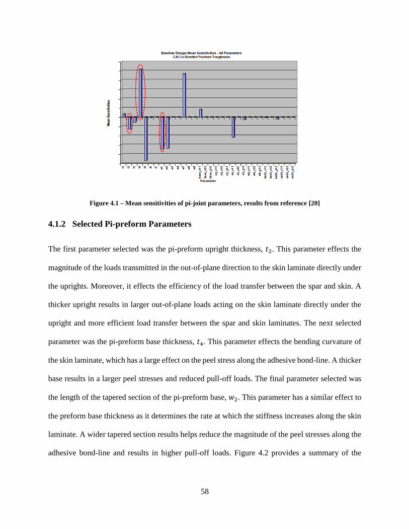
58

Figure 4.1 – Mean sensitivities of pi-joint parameters, results from reference [20]

4.1.2 Selected Pi-preform Parameters

The first parameter selected was the pi-preform upright thickness, 𝑡2. This parameter effects the

magnitude of the loads transmitted in the out-of-plane direction to the skin laminate directly under

the uprights. Moreover, it effects the efficiency of the load transfer between the spar and skin. A

thicker upright results in larger out-of-plane loads acting on the skin laminate directly under the

upright and more efficient load transfer between the spar and skin laminates. The next selected

parameter was the pi-preform base thickness, 𝑡4. This parameter effects the bending curvature of

the skin laminate, which has a large effect on the peel stress along the adhesive bond-line. A thicker

base results in a larger peel stresses and reduced pull-off loads. The final parameter selected was

the length of the tapered section of the pi-preform base, 𝑤2. This parameter has a similar effect to

the preform base thickness as it determines the rate at which the stiffness increases along the skin

laminate. A wider tapered section results helps reduce the magnitude of the peel stresses along the

adhesive bond-line and results in higher pull-off loads. Figure 4.2 provides a summary of the

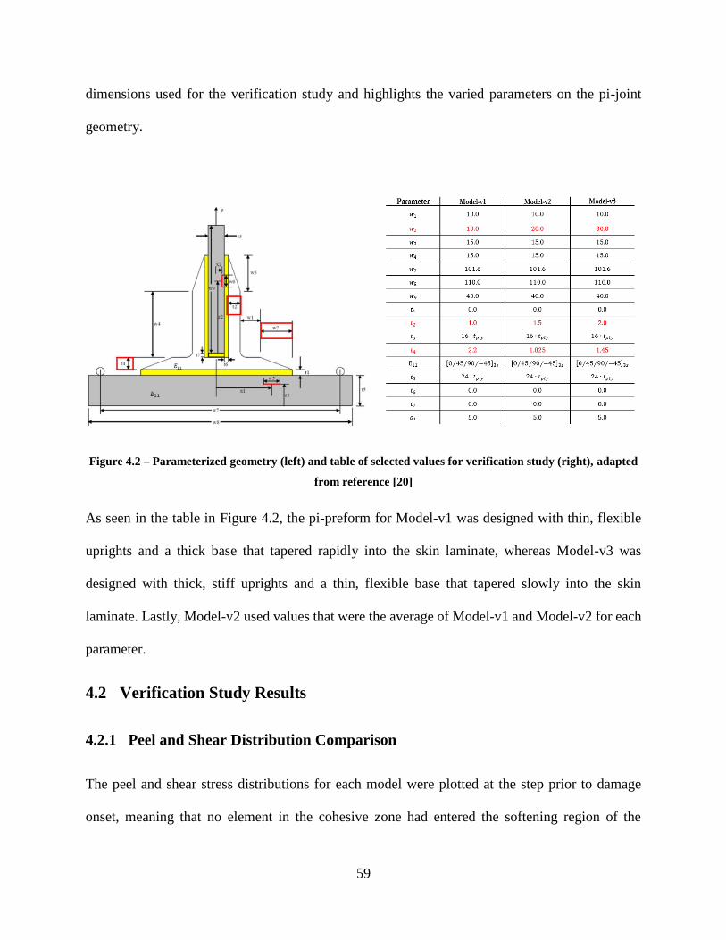
59

dimensions used for the verification study and highlights the varied parameters on the pi-joint

geometry.

Figure 4.2 – Parameterized geometry (left) and table of selected values for verification study (right), adapted

from reference [20]

As seen in the table in Figure 4.2, the pi-preform for Model-v1 was designed with thin, flexible

uprights and a thick base that tapered rapidly into the skin laminate, whereas Model-v3 was

designed with thick, stiff uprights and a thin, flexible base that tapered slowly into the skin

laminate. Lastly, Model-v2 used values that were the average of Model-v1 and Model-v2 for each

parameter.

4.2 Verification Study Results

4.2.1 Peel and Shear Distribution Comparison

The peel and shear stress distributions for each model were plotted at the step prior to damage

onset, meaning that no element in the cohesive zone had entered the softening region of the

60

traction-separation law. The point on the global load-displacement curves at which the stress

distributions were recorded are provided in Table 4-1. Note that the load is reported in per

millimeter width and equivalent load for a 50mm test specimen, because the models built for the

study were only 5mm wide, but a typical test specimen is 50mm wide.

Table 4-1 – Global load-displacement values at step prior to damage onset

Displacement

(mm) Load (N/mm)

Load for 50mm

Specimen (N)

Model-v1 0.76 28.02 1400.95

Model-v2 1.50 63.57 3178.39

Model-v3 4.24 173.37 8668.35

The peel and shear stress distributions are shown in Figure 4.3. Evaluating the stress distribution

in the adhesive bond-line, the effects of the selected parameters are evident. Model-v1 had the

highest peel stress at the edges of the pi-preform, even though the global applied load was roughly

one-sixth that of Model-v3. This is related to the pi-preform base thickness and taper distance,

parameters 𝑡4 and 𝑤2, respectively. Model-v1 had the highest value of 𝑡4 and lowest value of 𝑤2.

This resulted in a sudden change in stiffness along the skin laminate, which correlated to a local

change in the bending curvature and a spike in the peel stress. Conversely, the flexible pi-base of

Model-v3 allowed for a gradual change in stiffness along the skin laminate and reduced the

magnitude of the peel stress at the edges of the pi-preform. Finally, the effect of the pi-preform

upright thickness 𝑡2 can be observed from the spikes in the peel stress directly under the uprights.

61

Figure 4.3 – Stress distribution along bond-line between pi-preform and skin laminate

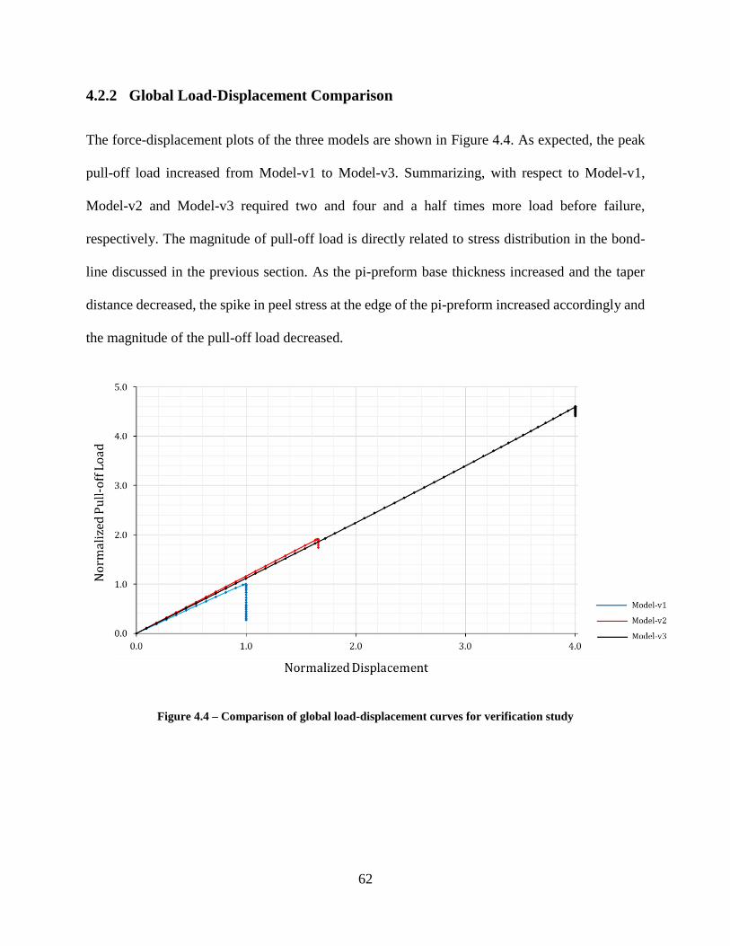
62

4.2.2 Global Load-Displacement Comparison

The force-displacement plots of the three models are shown in Figure 4.4. As expected, the peak

pull-off load increased from Model-v1 to Model-v3. Summarizing, with respect to Model-v1,

Model-v2 and Model-v3 required two and four and a half times more load before failure,

respectively. The magnitude of pull-off load is directly related to stress distribution in the bond-

line discussed in the previous section. As the pi-preform base thickness increased and the taper

distance decreased, the spike in peel stress at the edge of the pi-preform increased accordingly and

the magnitude of the pull-off load decreased.

Figure 4.4 – Comparison of global load-displacement curves for verification study

63

5. PRESENT WORK

The present work considered a composite pi-joint test specimen subject to pull-off load and

compared the predicted pull-off loads and damage paths of two discrete damage modeling tools.

The discrete damage modeling tools used were Abaqus XFEM with a LaRC05 built-in user

subroutine and BSAM. To demonstrate the effect of modeling intralaminar damage, baseline

models that only accounted for interface damage were included. Moreover, the skin laminate

stacking sequences was varied to determine the effect of stacking sequence on pull-off load and

predicted damage paths.

Between the present work and the verification study, a significant number of models needed to be

generated. To expedite the required pre-processing and eliminate user error in the model setup, a

python tool was developed to automate this process. Further detail on the developed python tool

is included in this section.

5.1 Selection of Parameters

5.1.1 Penalty Stiffness Selection

As outlined in Section 3.3.4, there is no clear definition of what the penalty stiffness should be,

and a large range of values can be used with almost no effect on the accuracy of the solution.

However, Turon showed in [13] that higher values of penalty stiffness require more Newton-

Raphson iterations and sporadic oscillations are apparent in the results. Thus, for the present work,

the goal was to select the penalty stiffness such that it was as low as possible while having

negligible contribution to the structure’s compliance. Substituting the material properties for IM7-

8552 into Equation 3.3.48 yield a penalty stiffness of 5.0𝐸6 N/mm for 𝛼 = 50. Therefore, a

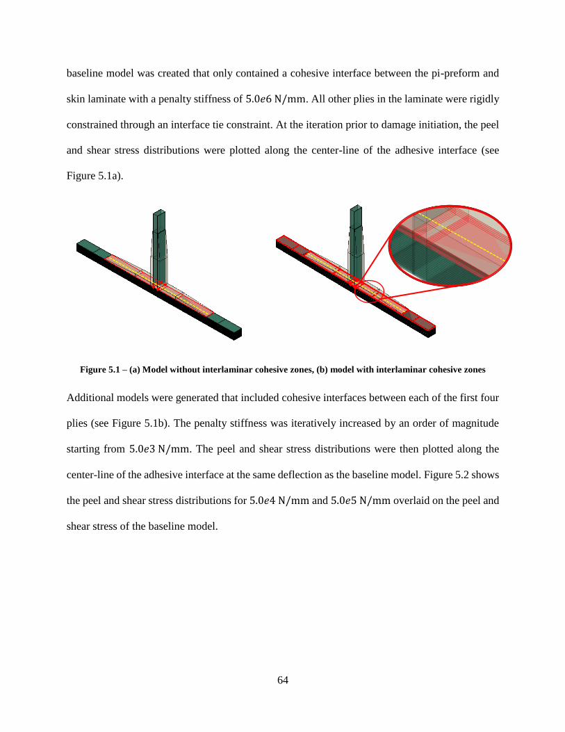
64

baseline model was created that only contained a cohesive interface between the pi-preform and

skin laminate with a penalty stiffness of 5.0𝑒6 N/mm. All other plies in the laminate were rigidly

constrained through an interface tie constraint. At the iteration prior to damage initiation, the peel

and shear stress distributions were plotted along the center-line of the adhesive interface (see

Figure 5.1a).

Figure 5.1 – (a) Model without interlaminar cohesive zones, (b) model with interlaminar cohesive zones

Additional models were generated that included cohesive interfaces between each of the first four

plies (see Figure 5.1b). The penalty stiffness was iteratively increased by an order of magnitude

starting from 5.0𝑒3 N/mm. The peel and shear stress distributions were then plotted along the

center-line of the adhesive interface at the same deflection as the baseline model. Figure 5.2 shows

the peel and shear stress distributions for 5.0𝑒4 N/mm and 5.0𝑒5 N/mm overlaid on the peel and

shear stress of the baseline model.

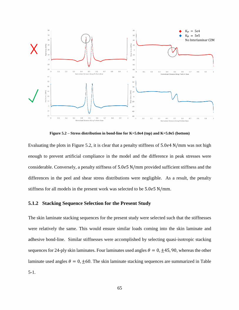
65

Figure 5.2 – Stress distribution in bond-line for K=5.0e4 (top) and K=5.0e5 (bottom)

Evaluating the plots in Figure 5.2, it is clear that a penalty stiffness of 5.0𝑒4 N/mm was not high

enough to prevent artificial compliance in the model and the difference in peak stresses were

considerable. Conversely, a penalty stiffness of 5.0𝑒5 N/mm provided sufficient stiffness and the

differences in the peel and shear stress distributions were negligible. As a result, the penalty

stiffness for all models in the present work was selected to be 5.0𝑒5 N/mm.

5.1.2 Stacking Sequence Selection for the Present Study

The skin laminate stacking sequences for the present study were selected such that the stiffnesses

were relatively the same. This would ensure similar loads coming into the skin laminate and

adhesive bond-line. Similar stiffnesses were accomplished by selecting quasi-isotropic stacking

sequences for 24-ply skin laminates. Four laminates used angles 휃 = 0,±45, 90, whereas the other

laminate used angles 휃 = 0,±60. The skin laminate stacking sequences are summarized in Table

5-1.

66

Table 5-1 – Stacking sequences for the present work

Stacking Sequence Wing Skin Coordinate

Sys

Pi-joint Test Specimen

Coordinate Sys.

A [0 45⁄ 90⁄ −45⁄ ]3𝑠 [90 −45⁄ 0⁄ 45⁄ ]3𝑠

B [45 0⁄ −45⁄ 90⁄ ]3𝑠 [−45 90⁄ 45⁄ 0⁄ ]3𝑠

C [60 0⁄ −60⁄ ]4𝑠 [−30 90⁄ 30⁄ ]4𝑠

D [90 −45⁄ 0⁄ 45⁄ ]3𝑠 [0 45⁄ 90⁄ −45⁄ ]3𝑠

E [0𝐹 45⁄ 90⁄ −45⁄ ]3𝑠 [0𝐹 −45⁄ 0⁄ 45⁄ ]3𝑠

*Stacking sequences D and E were not able to be included in the present work .

Note that while the wing skin stacking sequences were defined in the wing skin coordinate system

for entry into the python tool, the stacking sequence aligned with the primary loading direction for

the pi-joint pull-off tests are rotated 90° about the laminate z-axis. Therefore, the stacking

sequences that will be referenced in the results section will be those in the right most column of

Table 5-1. Please refer to Figure 5.8 for coordinate system definitions.

These stacking sequences were selected with care and the reasoning for each is as follows. Stacking

sequence A contains a ninety-degree surface ply with respect to the test specimen coordinate

system. This stacking sequence was selected to demonstrate how large of an effect ignoring bulk

material failure (i.e. matrix cracking) could have on the predicted pull-off loads. It was

hypothesized that a matrix crack would quickly initiate at the termination of the pi-preform and

result in a large reduction in pull-off load. Stacking sequence’s B and D were selected to compare

with the results of stacking sequence A when an angled or zero-degree ply was the surface ply.

Stacking sequence E was selected to model the common practice of applying a woven material to

the outer most plies of a laminate. Finally, stacking sequence C was selected to demonstrate the

effect of maximizing the interlaminar stress by using lamina orientations with the largest Poisson’s

mismatch and coefficient of mutual influence mismatch. For readers that are not familiar with the

67

effects of these mismatch’s please see reference [30]. In short, maximizing the mismatch of these

parameters results in maximizing the interlaminar stresses and greatly increases the chances of

free-edge delamination.

Note that stacking sequence’s D and E highlighted in red in Table 5-1 were not able to be

completed due to an unforeseen failure of computing resources. However, it was important to

include these stacking sequences in this section to communicate the author’s intent for the present

work.

5.2 Model Generation

5.2.1 Python Tool

A python tool was developed for this work to automate the required preprocessing tasks. For the

Abaqus models, the tool was used for all preprocessing tasks and the models were ready for

submission once the script completed. For the BSAM models, the tool could only be used to

generate the geometry and mesh definition and all other preprocessing task had to be completed in

the BSAM GUI or using additional python scripts that operated on the BSAM input files. The

python tool used in the present work is included in Appendix A.

Parametric Geometry

Figure 5.3 provides a schematic of a parameterized pi-joint test specimen. All geometric

dimensions denoted by 𝑤𝑖, 𝑡𝑖 and ℎ𝑖 were parameters that could be varied using the python tool.

The provided dimensions were then used to compute the parametric datums shown on the right

side of Figure 5.3.

68

Figure 5.3 – Parameterized geometry and datums for python tool

It is important to note that all geometric parameters were defined explicitly except for the skin and

spar laminate thicknesses, 𝑡1 and 𝑡2, respectively. These geometric features were computed from

the defined stacking sequence and ply thickness data. Therefore, after the ply thickness data, skin

and spar laminate stacking sequence’s and remaining geometric parameters shown in Figure 5.3

were provided, the pi-joint geometry was fully defined and the python tool could be executed.

Parametric Mesh

Like the geometry, the mesh definition was also parametrized. The relative element size in each

section of the pi-joint model was defined as a function of the ply thickness. All sections with a

different color in Figure 5.4 could have been defined with a different mesh density. This feature

allowed the mesh to be easily optimized and refined to obtain a converged solution.

69

Figure 5.4 – Sectioned pi-joint for mesh density specification using python tool

Additional advanced meshing functionality was programed into the tool that allowed for bias

seeding and local mesh refinement options. For the models generated for the present work, bias

seeding was only used in the beige section in Figure 5.4. The local refinement tool could be used

to accurately predict damage initiation in a local area, but damage progression would be in accurate

as the damage propagated out of the refined location.

Material Input

In addition to the geometric and mesh inputs described previously, the python tool requires

definitions of the material properties for the material system used for the skin and spar laminates.

Furthermore, homogenized orthotropic properties for the pi-preform and the cohesive zone

properties/parameters defined in Section 3.3. After the geometry, mesh, and material inputs are

provided the python tool is ready to be executed.

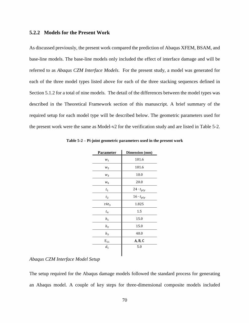
70

5.2.2 Models for the Present Work

As discussed previously, the present work compared the prediction of Abaqus XFEM, BSAM, and

base-line models. The base-line models only included the effect of interface damage and will be

referred to as Abaqus CZM Interface Models. For the present study, a model was generated for

each of the three model types listed above for each of the three stacking sequences defined in

Section 5.1.2 for a total of nine models. The detail of the differences between the model types was

described in the Theoretical Framework section of this manuscript. A brief summary of the

required setup for each model type will be described below. The geometric parameters used for

the present work were the same as Model-v2 for the verification study and are listed in Table 5-2.

Table 5-2 – Pi-joint geometric parameters used in the present work

Parameter Dimension (mm)

𝑤1 101.6

𝑤2 101.6

𝑤3 10.0

𝑤4 20.0

𝑡1 24 ∙ 𝑡𝑝𝑙𝑦

𝑡2 16 ∙ 𝑡𝑝𝑙𝑦

𝑡4𝑡3 1.825

𝑡4 1.5

ℎ1 15.0

ℎ2 15.0

ℎ3 40.0

E11 A, B, C

𝑑1 5.0

Abaqus CZM Interface Model Setup

The setup required for the Abaqus damage models followed the standard process for generating

an Abaqus model. A couple of key steps for three-dimensional composite models included

71

ensuring material orientations were correctly defined and ply interfaces were properly constrained

to avoid rigid body motion in the analysis. For the ply interfaces that did not consider damage, the

interfaces were rigidly tied together using the Abaqus tie constraint. For the ply interfaces that

included damage, the interface tie constraint was replaced with a cohesive contact interaction. The

details of the cohesive zone model and cohesive zone properties were defined within an interaction

property that was selected when generating the cohesive contact interaction.

For the Abaqus CZM Interface models the cohesive contact interaction was defined for the

adhesive bond-line between the pi-preform and skin laminate as well as the interfaces between

each of the top four plies. The interface damage was constrained to the top four plies based on

observation of failures during physical testing that were conveyed to the author by experienced

personnel. Figure 5.5 provides a depiction of the of Abaqus CZM Interface models and where the

cohesive interfaces were applied.

Figure 5.5 – Schematic of Abaqus CZM Interface models (base-line models)

Cohesive zone

interfaces

72

Abaqus XFEM Model Setup

The Abaqus XFEM models followed the same process for the defining the cohesive interfaces,

however, for the XFEM models, an XFEM zone had to be defined where the elements were

duplicated to provide the additional degrees of freedom required for modeling discontinuities in

the displacement field. Like the interface damage, the intralaminar damage was confined to the

top four plies and only extended slightly beyond the termination of the pi-preform. Figure 5.6

provides a depiction of the of Abaqus XFEM models and where the cohesive interfaces and XFEM

defined zones were applied.

Figure 5.6 – Schematic of Abaqus XFEM models

Moreover, the present work implemented the LaRC05 built-in subroutine available in Abaqus.

This subroutine is a new feature and has not yet been integrated into the GUI. The subroutine was

automatically called when the material in the XFEM zone began with the string,

“ABQ_LARC05_DMGINI”. Additionally, there was no form in the GUI that contained the fields

XFEM Defined

Zone Cohesive zone

interfaces

73

for inputting the required material properties, therefore, the input file was directly edited so that

the material was properly defined, and the subroutine could be executed.

BSAM Models

BSAM is a research code used specifically for modeling progressive damage in composite

structures, therefore, the process for setting up a model did not have the added benefits of the

developed commercial code Abaqus. However, BSAM was designed to read Abaqus input files

for the geometry and mesh definitions. Therefore, the python tool was used for the geometry and

mesh definition, which saved a considerable amount time. The BSAM GUI was then used to

create an input file for one model and an additional python script was used to modify the input file

for the different stacking sequences.

After the geometry and mesh are defined, the remaining steps can be explained best with the aid

of Figure 5.7. Let the discretized geometry be referred to as the Analysis Domain. For BSAM

models, the analysis domain is divided into element clusters, which are analogous to a part in

Abaqus. At the cluster level, material assignments are applied, and MIC enriched or RxFEM zones

are defined. Specific clusters or specific sections of clusters may be excluded from the MIC

enriched domain. Clusters that are included in the MIC enriched domain require lamina strength

properties for the insertion of matrix cracks via the LaRC04 failure criteria, and cohesive zone

properties defined for matrix crack propagation. Within each cluster node sets are defined that are

used to define material orientations, boundary conditions, and connections between neighboring

clusters. Connections can be defined strictly as penalty based to maintain displacement continuity

across cluster interfaces, or using cohesive zones to model the kinematics of the displacement

jumps across cluster interfaces during delamination. If a connection is defined using a cohesive

zone, the appropriate cohesive zone properties must be assigned to the connection.

74

Figure 5.7 – Preprocessing Diagram for BSAM models

For the present work, a cluster was defined for each ply in the skin and spar laminates and for the

pi-preform. Like the Abaqus models, the enriched domain was constrained to the top four plies,

however, the cohesive interfaces were defined between each cluster in the model. Table 5-3

provides a summary of the three model types and the damage mechanisms that are captured.

Table 5-3 – Summary of model types and damage captured

Model Type Interlaminar

Damage Intralaminar

Damage

Abaqus CZM Interface x

Abaqus XFEM x x

BSAM x x

5.3 Modeling Details

Material Properties

The IM7-8552 unidirectional material system was used for the skin and spar laminates for all

models presented in this work. This system was selected based on availability of material

75

properties and its wide range use in the aerospace industry. The pi-preform was modeled using

orthotropic homogenous properties that were approximated from IM7-8552 plain weave fabric

properties. To account for the effects of the three-dimensional weaving pattern, the through-the-

thickness plain weave stiffness was slightly increased, and in-plane stiffness was slightly reduced.

Table 5-4, provides a summary of the material properties used in the current work. Note that failure

in the pi-preform was not consider, therefore, only the stiffness properties were required to obtain

the loads acting on the skin laminate.

Table 5-4 – Material properties used in the present work

Unidirectional Plain Weave Preform (Approx)

Fiber Direction Tensile Modulus, 𝐸11(GPa) 161.00 71.70 65.00

Transverse Tensile Modulus, 𝐸22(GPa) 11.38 71.70 65.00

Through-Thickness Tensile Modulus, 𝐸33(GPa) 11.38 10.30 30.00

Poisson’s Ratio, 𝜈12 0.320 0.04 0.12

Poisson’s Ratio, 𝜈13 0.320 0.35 0.30

Poisson’s Ratio, 𝜈23 0.436 0.35 0.30

In-plane Shear Modulus, 𝐺12(GPa) 5.17 4.48 4.40

Transverse Shear Modulus, 𝐺13(GPa) 5.17 4.14 4.25

Transverse Shear Modulus, 𝐺23(GPa) 3.98 4.14 4.25

Tensile/Comp Strength Fiber Direction 𝑌𝑡/𝑌𝑐 (MPa) 2400/1785 N/A N/A

Transverse Tensile/Comp Strength 𝑌𝑡/𝑌𝑐 (MPa) 100/290 N/A N/A

Shear Strength 𝑆12 (MPa) 98 N/A N/A

As outlined in Section 3.3, additional material properties are required for modeling crack

propagation using CZM. IM7-8552 has been a common material system used for this type of

analysis, therefore, the required properties were readily available. For the adhesive, generic

properties were used. The interface material properties used for IM7-8552 and the generic adhesive

are listed in Table 5-5.

76

Table 5-5 – Material properties used to define cohesive zones

IM7-8552 Adhesive

Mode I Strength, 𝑌𝑜 (MPa) 62.0 62.0

Mode II Strength, 𝑆𝑜 (MPa) 93.0 93.0

Mode I Fracture Toughness, 𝐺𝐼𝐶 (kJ/m2 ) 0.240 0.500

Mode II Fracture Toughness, 𝐺𝐼𝐼𝐶 (kJ/m2 ) 0.739 1.500

Overview of CZM Models

Cohesive zone models are used explicitly by the tools in this work to model govern delamination

and matrix crack propagation. Note that the cohesive zone models used in Abaqus and BSAM are

slightly different. The primary difference is the criteria for damage initiation. Abaqus uses the

quadratic traction criteria for predicting damage initiation in the cohesive zone, whereas BSAM

uses an equivalent interlaminar strength as defined by Turon [13]. Table 5-6 provides a summary

of the cohesive zone models that were used in Abaqus and BSAM for the current work. For full

details on the formulation of the cohesive zone models outlined in Table 5-6, the reader is referred

to Section 3.3.5.

Table 5-6 – Cohesive zone model comparison for Abaqus and BSAM

Required

Properties Abaqus CZM [12] BSAM CZM [13]

Damage Initiation Criteria 𝑌𝑜 , 𝑆𝑜 (⟨𝜏3⟩

𝑁)

2

+ (𝜏2𝑆)2

+ (𝜏1𝑇)2

= 1 (𝜏𝑜(𝐵))2= 𝑌𝑜

2 + (𝑆𝑜2 − 𝑌𝑜

2)𝐵𝜂

Damage Evolution Type N/A Energy Energy

Damage Evolution Softening N/A Linear Linear

Mixed-Mode Fracture Toughness [31]

𝐺𝐼𝐶 , 𝐺𝐼𝐼𝐶 𝐺𝐶(𝐵) = 𝐺𝐼𝐶 + (𝐺𝐼𝐼𝐶 − 𝐺𝐼𝐶)𝐵𝜂 𝐺𝐶(𝐵) = 𝐺𝐼𝐶 + (𝐺𝐼𝐼𝐶 − 𝐺𝐼𝐶)𝐵

𝜂

Power (휂) N/A 2.17 2.17

77

Coordinate System Definitions

In the current work, the coordinate system definitions are different for the skin laminate, spar

laminate and pi-joint test specimen. The coordinate system for defining the skin laminate stacking

sequences is defined with the x-axis along the primary axis of the wing and the z-axis pointing

upward. The coordinate system for defining the spar laminate stacking sequence is the skin

coordinate system rotated 90° about the x-axis. Note that these were the referenced coordinate

systems when the wing skin and spar stacking sequences were entered into the python tool that

generated the Abaqus models. Finally, the coordinate system for the pi-joint test specimen is

defined with the x-axis aligned with the primary bending axis of the skin laminate, which is the

skin coordinate system rotated 90° about the z-axis. For clarification refer to Figure 5.8, where the

coordinate system definitions are clearly defined.

Figure 5.8 – Coordinate system definitions

𝒙 𝒚

𝒛

𝒙

𝒚 𝒛

𝒙 𝒚

𝒛

pi-joint test specimen coordinate sys

wing skin coordinate sys

spar coordinate sys

78

6. RESULTS

Within this chapter the results for present work are presented. First, a mesh convergence study is

presented to show the mesh selected for the study is relatively insensitive to the mesh. Next, the

predicted damage progression is presented for stacking sequences A, B and C for each of the three

model types followed by a comparison of the global load-displacement curves.

6.1 Mesh Convergence Study

A mesh refinement study was performed to ensure that the solutions obtained had converged

within an acceptable tolerance. Equation 6.1.1 was used to estimate the length of the cohesive zone

and generate a range of element sizes for the refinement study. The selected element sizes

considered the recommendation of Turon that between three and ten elements should be used in

the cohesive zone [13].

𝑙𝑐𝑧 =𝐸𝐺𝐶𝜏𝑜2

(6.1.1)

In the present work, two materials are represented by zero-thickness cohesive elements. The

adhesive between the pi-preform and the skin laminate and the lamina interlaminar region. The

length of the cohesive zone is directly proportional to the fracture toughness and inversely

proportional to the square of the cohesive strength. The two materials used have the same strength

properties, however, the fracture toughness of the adhesive material is approximately twice the

interlaminar fracture toughness. This infers that the required refinement will be governed by the

interlaminar properties. Still, the refinement study was performed for both materials and the results

were compared. Table 6-1, presents the relative element size that is input into the python tool to

79

generate the mesh and the corresponding number of elements in the cohesive zone for each set of

material properties.

Table 6-1 – Mesh densities for mesh convergence study

Relative

Element Size 𝐍𝐚𝐝𝐡𝐯 𝐍𝐥𝐚𝐦

6 ∙ tply 1.7 N/A

5 ∙ tply 2.1 N/A

4 ∙ tply 2.6 1.3

3 ∙ tply 3.5 1.7

2 ∙ tply 5.2 2.6

tply 10.4 5.1

0.5 ∙ tply N/A 10.3

The refinement study was performed using only a single cohesive zone between the pi-preform

and the skin laminate as shown in Figure 6.11. The peak loads for each mesh density were

normalized by peak load of the mesh with the highest level of refinement. The percent increase in

peak load was then plotted against the number of elements in the cohesive zone to obtain the

convergence curves shown in Figure 6.1.

Figure 6.1 – Mesh convergence plots

𝐺adhv

𝐺lam

80

The relative element size for the study was selected by evaluating the mesh convergence curves

and weighing the computational cost of increased refinement. At a relative element size of twice

the ply thickness, the models contained 600k degrees of freedom. With the available computing

power and time to complete the study this was determined to be the upper bound for the model

size. Therefore, the selected relative element size was twice the ply thickness. Note that the points

that correlate to the selected element size on the mesh convergence curves are highlighted in red.

6.2 Abaqus XFEM and BSAM Comparison

Presentation of Results

In this section, the results of the Abaqus XFEM and BSAM models for stacking sequences A, B

and C are presented and compared to the baseline Abaqus Interface CZM models. The format for

presenting the results is as follows. A top-view of the first four plies in region under the pi-preform

will be shown with a capture of the final damage state for each model type. The damage

progression will be explained in detail from initiation to final failure for each of the model types.

Then a comparison of the global load-displacement plots will be presented accompanied by a brief

discussion.

Figure 6.2 provides a schematic of the location that the damage captures are pulled from. Note

that the contour plots in the damage captures will be of the interface damage and a red element

denotes that the delamination has propagated through that element. The matrix cracks or

intralaminar damage will be highlighted with a bounding box. Moreover, the damage captures are

from a top-view, therefore the interface damage contour is for the interface between the shown ply

and the ply above. The corresponding ply numbers and ply interfaces are clearly designated in

Figure 6.2 below.

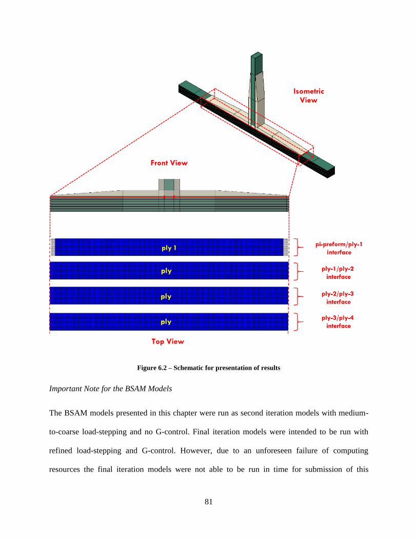
81

Figure 6.2 – Schematic for presentation of results

Important Note for the BSAM Models

The BSAM models presented in this chapter were run as second iteration models with medium-

to-coarse load-stepping and no G-control. Final iteration models were intended to be run with

refined load-stepping and G-control. However, due to an unforeseen failure of computing

resources the final iteration models were not able to be run in time for submission of this

Isometric View

Front View

Top View

ply 1

ply

ply

ply

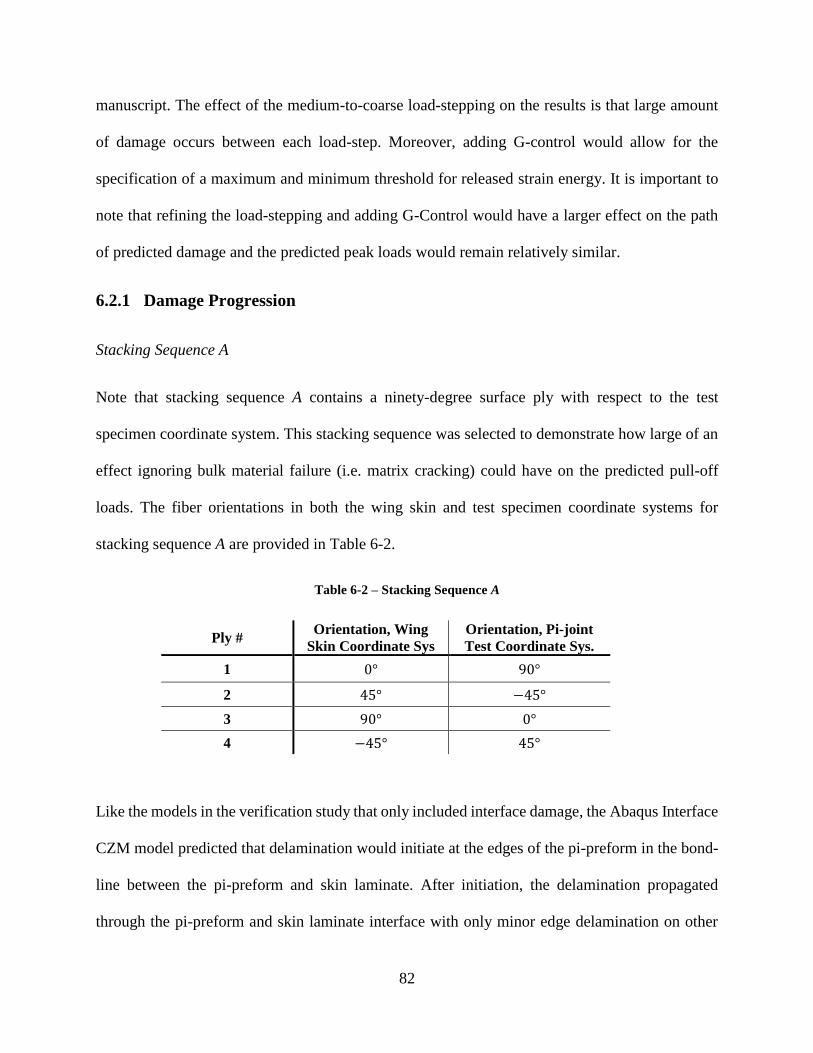
82

manuscript. The effect of the medium-to-coarse load-stepping on the results is that large amount

of damage occurs between each load-step. Moreover, adding G-control would allow for the

specification of a maximum and minimum threshold for released strain energy. It is important to

note that refining the load-stepping and adding G-Control would have a larger effect on the path

of predicted damage and the predicted peak loads would remain relatively similar.

6.2.1 Damage Progression

Stacking Sequence A

Note that stacking sequence A contains a ninety-degree surface ply with respect to the test

specimen coordinate system. This stacking sequence was selected to demonstrate how large of an

effect ignoring bulk material failure (i.e. matrix cracking) could have on the predicted pull-off

loads. The fiber orientations in both the wing skin and test specimen coordinate systems for

stacking sequence A are provided in Table 6-2.

Table 6-2 – Stacking Sequence A

Ply # Orientation, Wing

Skin Coordinate Sys

Orientation, Pi-joint

Test Coordinate Sys.

1 0° 90°

2 45° −45°

3 90° 0°

4 −45° 45°

Like the models in the verification study that only included interface damage, the Abaqus Interface

CZM model predicted that delamination would initiate at the edges of the pi-preform in the bond-

line between the pi-preform and skin laminate. After initiation, the delamination propagated

through the pi-preform and skin laminate interface with only minor edge delamination on other

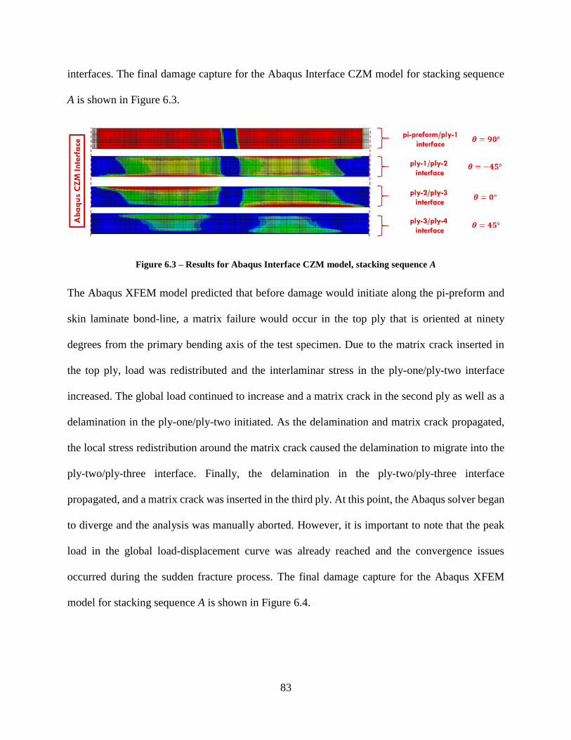
83

interfaces. The final damage capture for the Abaqus Interface CZM model for stacking sequence

A is shown in Figure 6.3.

Figure 6.3 – Results for Abaqus Interface CZM model, stacking sequence A

The Abaqus XFEM model predicted that before damage would initiate along the pi-preform and

skin laminate bond-line, a matrix failure would occur in the top ply that is oriented at ninety

degrees from the primary bending axis of the test specimen. Due to the matrix crack inserted in

the top ply, load was redistributed and the interlaminar stress in the ply-one/ply-two interface

increased. The global load continued to increase and a matrix crack in the second ply as well as a

delamination in the ply-one/ply-two initiated. As the delamination and matrix crack propagated,

the local stress redistribution around the matrix crack caused the delamination to migrate into the

ply-two/ply-three interface. Finally, the delamination in the ply-two/ply-three interface

propagated, and a matrix crack was inserted in the third ply. At this point, the Abaqus solver began

to diverge and the analysis was manually aborted. However, it is important to note that the peak

load in the global load-displacement curve was already reached and the convergence issues

occurred during the sudden fracture process. The final damage capture for the Abaqus XFEM

model for stacking sequence A is shown in Figure 6.4.

84

Figure 6.4 – Results for Abaqus XFEM model, stacking sequence A

Like the Abaqus XFEM model, the BSAM model predicted a matrix failure would occur in the

top ply prior to a delamination of the pi-preform/ply-one interface. The matrix crack resulted in

load redistribution and the interlaminar stress in the ply-one/ply-two interface increased. The

global load continued to increase until a delamination initiated in the ply-one/ply-two interface.

The delamination propagated until a matrix crack was inserted in the second ply. At this point, the

delamination migrated to the ply-two/ply-three interface until the pi-preform and spar laminate

separated from the skin laminate. The final damage capture for the BSAM model for stacking

sequence A is shown in Figure 6.5.

Figure 6.5 – Results for BSAM model, stacking sequence A

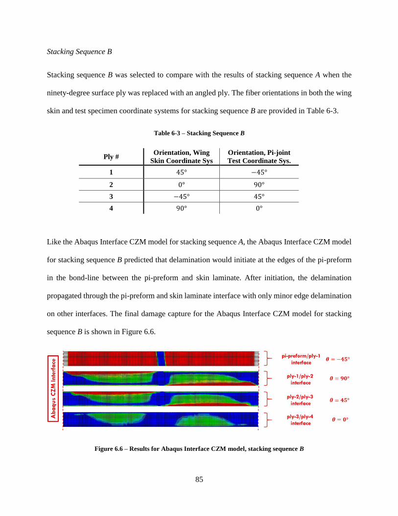
85

Stacking Sequence B

Stacking sequence B was selected to compare with the results of stacking sequence A when the

ninety-degree surface ply was replaced with an angled ply. The fiber orientations in both the wing

skin and test specimen coordinate systems for stacking sequence B are provided in Table 6-3.

Table 6-3 – Stacking Sequence B


Skin Coordinate Sys



1 45° −45°

2 0° 90°

3 −45° 45°

4 90° 0°

Like the Abaqus Interface CZM model for stacking sequence A, the Abaqus Interface CZM model

for stacking sequence B predicted that delamination would initiate at the edges of the pi-preform

in the bond-line between the pi-preform and skin laminate. After initiation, the delamination

propagated through the pi-preform and skin laminate interface with only minor edge delamination

on other interfaces. The final damage capture for the Abaqus Interface CZM model for stacking

sequence B is shown in Figure 6.6.

Figure 6.6 – Results for Abaqus Interface CZM model, stacking sequence B

86

For stacking sequence B, the Abaqus XFEM model predicted that damage initiation would occur

due to a matrix failure in the top ply oriented minus forty-five degrees from the primary bending

axis near the termination of the pi-preform. The localized redistribution of stress about the matrix

crack caused a delamination to initiate on the ply-one/ply-two interface. Concurrently, a

delamination in the pi-preform/ply-one interface initiated on the opposite side of the matrix crack.

The delamination in the pi-preform/ply-one interface propagated towards the pi-preform

termination point, whereas the delamination in the ply-one/ply-two interface propagated towards

center of the specimen. At this point, cracks oriented transverse to the fiber direction were inserted

into the second ply. It was concluded that this was not physically based and was a result of a

numerical error as the cracks should have remained parallel to the fibers. Moreover, the Abaqus

solver began to diverge and the analysis was manually aborted. It is important to note that the peak

load in the global load-displacement curve was already reached and the convergence issues

occurred during the sudden fracture process. The final damage capture for the Abaqus XFEM

model for stacking sequence B is shown in Figure 6.7.

Figure 6.7 – Results for Abaqus XFEM model, stacking sequence B

Like the Abaqus XFEM model, the BSAM model predicted a matrix failure would occur in the

top ply prior to a delamination of the pi-preform/ply-one interface. However, a matrix crack was

only inserted on one side of the joint and never inserted on the other side. A delamination initiated

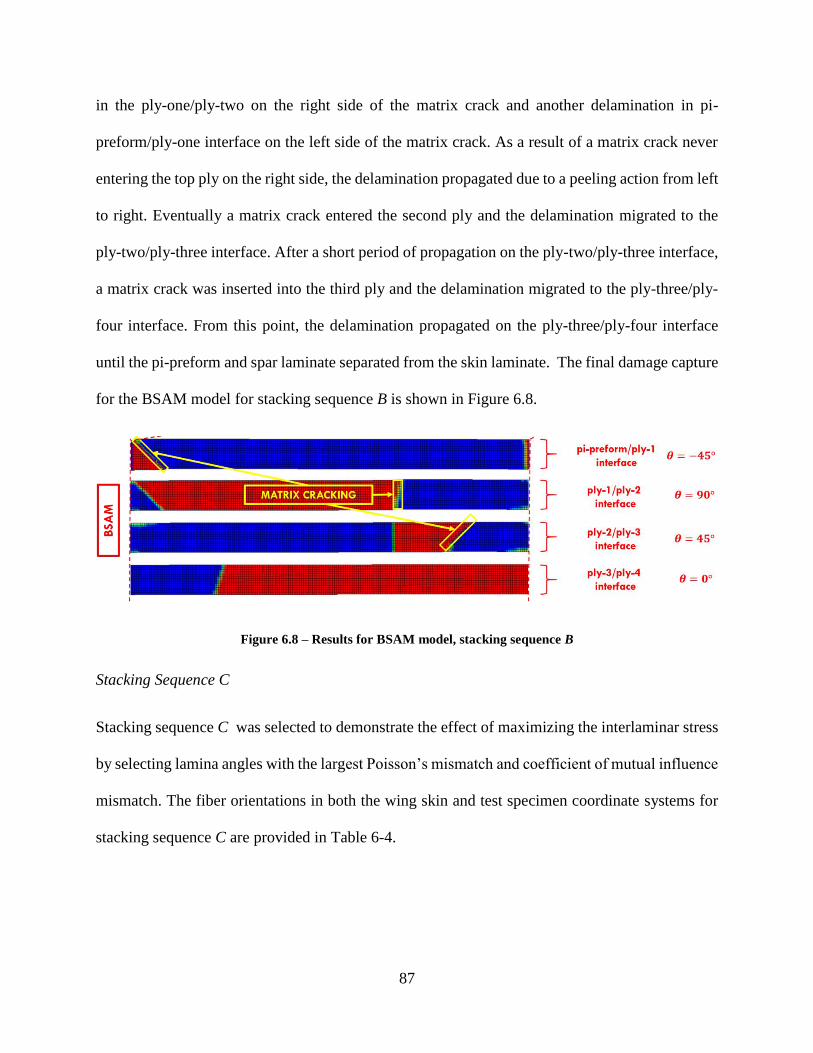
87

in the ply-one/ply-two on the right side of the matrix crack and another delamination in pi-

preform/ply-one interface on the left side of the matrix crack. As a result of a matrix crack never

entering the top ply on the right side, the delamination propagated due to a peeling action from left

to right. Eventually a matrix crack entered the second ply and the delamination migrated to the

ply-two/ply-three interface. After a short period of propagation on the ply-two/ply-three interface,

a matrix crack was inserted into the third ply and the delamination migrated to the ply-three/ply-

four interface. From this point, the delamination propagated on the ply-three/ply-four interface

until the pi-preform and spar laminate separated from the skin laminate. The final damage capture

for the BSAM model for stacking sequence B is shown in Figure 6.8.

Figure 6.8 – Results for BSAM model, stacking sequence B

Stacking Sequence C

Stacking sequence C was selected to demonstrate the effect of maximizing the interlaminar stress

by selecting lamina angles with the largest Poisson’s mismatch and coefficient of mutual influence

mismatch. The fiber orientations in both the wing skin and test specimen coordinate systems for

stacking sequence C are provided in Table 6-4.

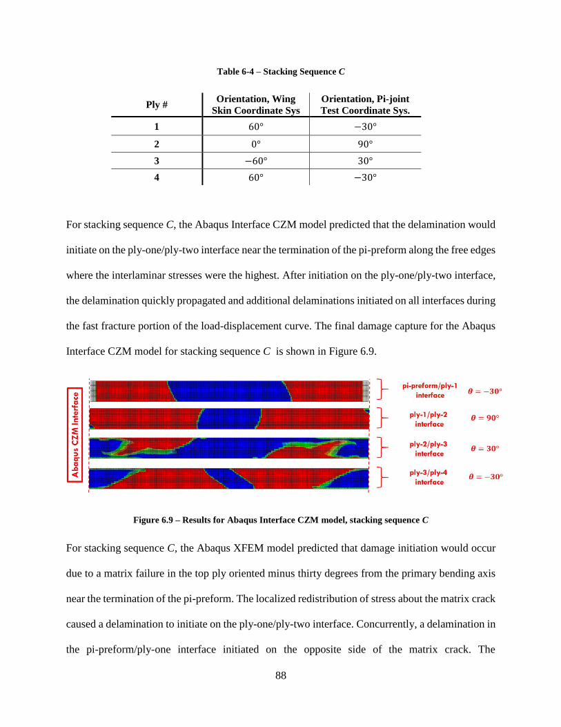
88

Table 6-4 – Stacking Sequence C


Skin Coordinate Sys



1 60° −30°

2 0° 90°

3 −60° 30°

4 60° −30°

For stacking sequence C, the Abaqus Interface CZM model predicted that the delamination would

initiate on the ply-one/ply-two interface near the termination of the pi-preform along the free edges

where the interlaminar stresses were the highest. After initiation on the ply-one/ply-two interface,

the delamination quickly propagated and additional delaminations initiated on all interfaces during

the fast fracture portion of the load-displacement curve. The final damage capture for the Abaqus

Interface CZM model for stacking sequence C is shown in Figure 6.9.

Figure 6.9 – Results for Abaqus Interface CZM model, stacking sequence C

For stacking sequence C, the Abaqus XFEM model predicted that damage initiation would occur

due to a matrix failure in the top ply oriented minus thirty degrees from the primary bending axis

near the termination of the pi-preform. The localized redistribution of stress about the matrix crack

caused a delamination to initiate on the ply-one/ply-two interface. Concurrently, a delamination in

the pi-preform/ply-one interface initiated on the opposite side of the matrix crack. The

89

delamination in the pi-preform/ply-one interface propagated towards the pi-preform termination

point, whereas the delamination in the ply-one/ply-two interface propagated towards center of the

specimen. Again, cracks oriented transverse to the fiber direction were inserted into the second ply

which were a result of numerical error. At this point, the Abaqus solver began to diverge and the

analysis was manually aborted. Again, the peak load in the global load-displacement curve was

already reached and the convergence issues occurred during the sudden fracture process. The final

damage capture for the Abaqus XFEM model for stacking sequence C is shown in Figure 6.10.

Figure 6.10 – Results for Abaqus XFEM model, stacking sequence C

Like the Abaqus XFEM model, the BSAM model predicted damage initiation would occur due to

a matrix failure in the top ply. BSAM also similarly predicted the initiation of delaminations on

either side of the matrix crack in the top ply for both the ply-one/ply-two interface and pi-

preform/ply-one interface. The delamination on the pi-preform/ply-one interface propagated

towards the termination of the pi-preform, whereas the delamination on the ply-one/ply-two

interface propagated towards the center of the specimen. Shortly after, a matrix crack was inserted

into the second ply and delamination migrated to the ply-two/ply-three interface. Eventually,

another matrix crack was inserted into the third ply and the delamination migrated to the ply-

three/ply-four interface until the pi-preform and spar laminate separated from the skin laminate.

The final damage capture for the BSAM model for stacking sequence C is shown in Figure 6.11.

90

Figure 6.11 – Results for BSAM model, stacking sequence C

6.2.2 Global Load-Displacement Comparison

The global load-displacement curves for stacking sequences A, B, and C are shown in Figure 6.12.

Each plot contains a curve for each of the three model types, Abaqus Interface CZM, Abaqus

XFEM and BSAM. For each stacking sequence, all load and displacement values are normalized

by the load and displacement values of the Abaqus Interface CZM model. Therefore, the predicted

peak loads of the discrete damage modeling tools can be read as a percentage of the base-line

model prediction. It is important to note that the slight differences in bending stiffness for the

Abaqus and BSAM models is due to the differences in element and geometric non-linear

formulations used. Abaqus uses selectively reduced eight-node elements and a hybrid updated

Lagrange non-linear formulation, whereas BSAM uses fully integrated eight-node elements and a

total Lagrange non-linear formulation.

Evaluating the plots in Figure 6.12, stacking sequence A showed a peak load reduction of 40-50%,

whereas stacking sequences B and C showed a reduction of 15-30%. Moreover, the peak load

predictions for the discrete damage modeling tools were within 10% for each stacking sequence

and less than 3% for stacking sequence C.

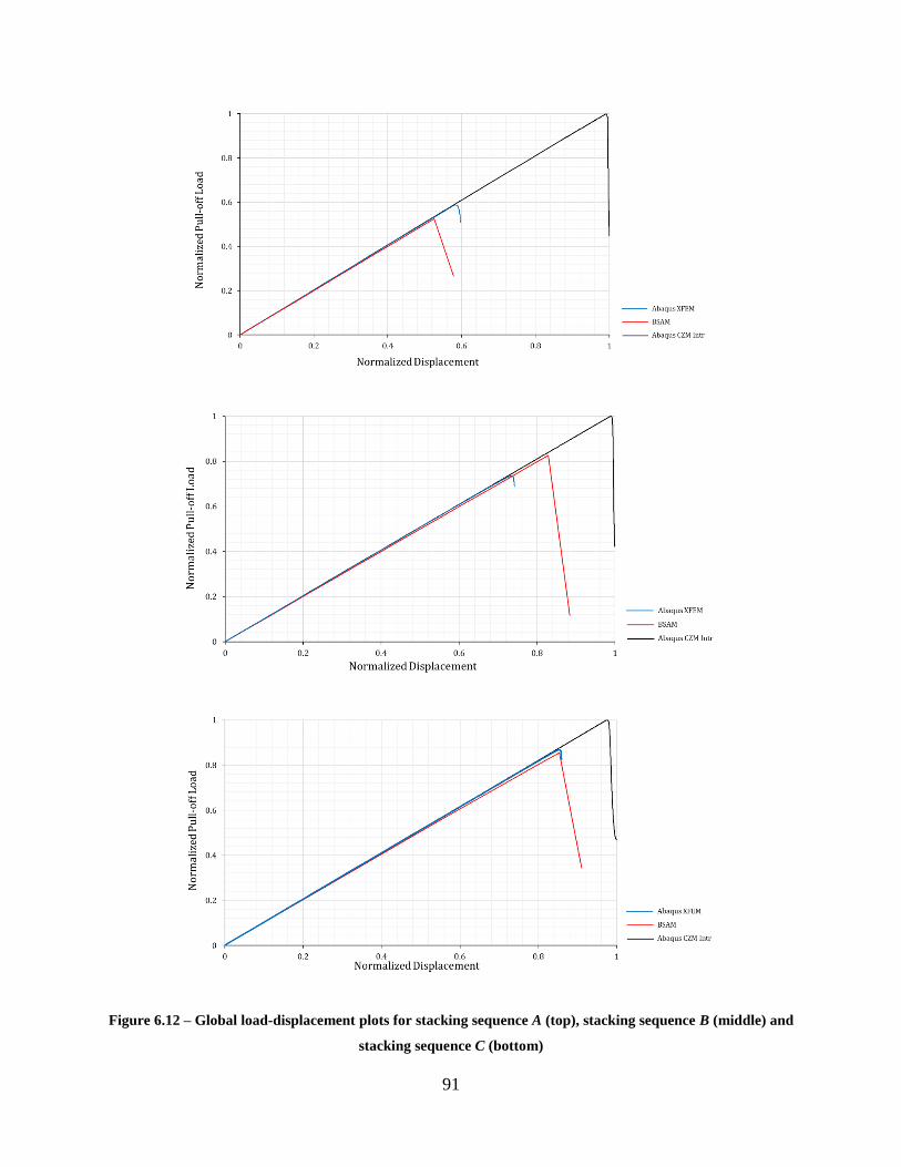
91

Figure 6.12 – Global load-displacement plots for stacking sequence A (top), stacking sequence B (middle) and

stacking sequence C (bottom)

92

7. CONCLUSIONS

The objective of the present work was to compare the predicted damage progression and pull-off

loads of two discrete damage modeling tools for a composite pi-joint test specimen subject to a

pull-off load. The pull-off loads and paths of predicted damage were recorded for three skin

laminate stacking sequences. Base-line models that only accounted for interface damage were

included to demonstrate the effect of intralaminar damage on the results. Prior to the present work,

a verification study was performed based on the conclusions of a parametric study to confirm

proper behavior of the pi-joint models. The predictions of the models built for the present work

were in agreement with the conclusions of the previous study. Due to the large number of models

required for the verification study and the present work, a python tool was developed to expedite

the required pre-processing and reduce user error. In the following sections conclusions will be

presented for the damage progression predictions, global load-displacement curves, and …

Synopsis of Predicted Damage Progression

Assessing the predicted damage paths for stacking sequences A, B, and C for each of the three

model types, the following conclusions were made. First, a strong correlation between matrix

cracking and delamination migration was present. In both the Abaqus XFEM and BSAM models,

the presence of matrix cracks appeared to terminate delaminations on one interface and migrate

them to the next interface in the stack. However, zero-degree plies were resistant to matrix cracking

and would mitigate the migration of delaminations. Moreover, the predicted damage initiation site

for the Abaqus XFEM and BSAM models were in agreement for all three stacking sequences and

the predicted damage paths were similar. Finally, the absence of matrix cracks in the base-line

models prevented delamination from migrating to the skin laminate interfaces for stacking

93

sequences A and B. This resulted in predicted failure along the adhesive bond-line where the

fracture toughness is approximately twice the interlaminar fracture toughness.

The damage progression for stacking sequence A were very similar with the primary difference

being the propagation of the delaminations before the next matrix crack was inserted and the

delamination migrated. It is not irrational to assume that by running the final iteration models with

refined load-stepping and G-control, that the propagation of delamination before the next matrix

crack was inserted would reduce. Moreover, the BSAM model for stacking sequence B never

inserted a matrix crack in the first ply on the right side of the joint. If this matrix crack was inserted

in the final iteration models, the predicted damage path would likely follow a similar progression

of the BSAM model for stacking sequence C. This assumption is supported by the fact that the

predicted damage paths of the Abaqus XFEM models for stacking sequences B and C were very

similar. The assumptions made in this paragraph are entirely speculation and would need to be

verified with future work.

Global Load-Displacement Comparison

The global load-displacement curves showed that including intralaminar damage significantly

affected the magnitude of the predicted pull-off loads. It was concluded that the failure mechanism

that lead to this reduction was matrix cracking that occurred in the top ply. Local stress

redistribution about the matrix cracks resulted in delaminations that initiated in the skin laminate

where the fracture toughness is about one-half the fracture toughness of the adhesive between the

pi-preform and skin laminate. Therefore, the delaminations reached a critical size at a lower peak

load and fast fracture of the specimen occurred. Next, as the angle of the top ply approached zero-

degrees, the reduction in pull-off load reduced and the predictions of the discrete damage modeling

94

tools approached the base-line model prediction. Future work that includes stacking sequences D

and E defined in chapter five would provide more definitive evidence for this conclusion.

Pros and Cons of the Discrete Damage Modeling Tools

The pros of Abaqus XFEM are primarily coupled to the fact that Abaqus is a well-established

commercial code. A well-establish commercial code comes well-developed pre and post

processing GUI’s and automation capabilities. One of the biggest advantages of the Abaqus XFEM

tool was the ability to completely automate the required pre-processing with the python tool,

whereas BSAM required more manual operation and tribal knowledge of the code for setting up a

proper analysis. Similarly, the post process capability of Abaqus made generating animations and

graphics easy. Additionally, Abaqus comes with a full element library that can be utilized in

different sections of the model. While this was not an advantage in the present work, it could be

used to reduce the model size and computational cost. Finally, Abaqus’s non-linear Newton-

Raphson procedure for their implicit solver automates the load-stepping increments based on a set

of defined variables. Conversely, BSAM requires the load-stepping to be defined by the user.

The pros of BSAM were primarily related to the capability of acquiring a converged solution. The

BSAM solver was able to obtain a converged solution for all stacking sequence in the present

work, whereas the Abaqus solver ran into convergence issues for all stacking sequences when

damage began to occur at multiple sites and the interaction became complex. Moreover, a large

amount of time was spent tuning the Abaqus solver to prevent convergence issues before the peak

loads were achieved. These included changing iteration criteria for step size reduction and

implementing line search algorithms for the Newton-Raphson solution procedure. Additionally,

BSAM only locally enriched the domain where cracks were inserted to save on computational

95

efficiency. Conversely, Abaqus required a XFEM domain to be defined and all elements in the

defined domain are duplicated doubling the size of the problem for the specified domain.

In end, both tools predicted the same location for damage initiation and had similar predictions for

initial damage progression and peak pull-off loads. However, the manual tuning required for the

Abaqus solver, convergence issues, and insertion of cracks transverse to the fiber direction raise

question to the current ability of Abaqus XFEM for progressive damage in composite structures.

Conversely, BSAM was able to obtain a converged solution with little effort of the user and has a

proven track-record for modeling progressive damage in composite structures.

96

REFERENCES

[1] Tavares, S. M. O., and Castro, P. M. S. T., An overview of fatigue in aircraft

structures. Fatigue & Fracture Engineering Materials & Structures, 40, 1510– 1529,

2017.

[2] Wanhill, R., Residual Strength Requirements for Aircraft Structures. 2017.

[3] Tsai, S. W., & Wu, E. M., A General Theory of Strength for Anisotropic Materials. Journal

of Composite Materials, 5(1), 58–80, 1971.

[4] Hashin, Z., Failure criteria for unidirectional fiber composites. Journal of Applied

Mechanics, Transactions ASME. 47, 329-334, 1980.

[5] Hinton, M. J., et al. Failure Criteria in Fibre Reinforced Polymer Composites: The World-

Wide Failure Exercise. Elsevier Science & Technology, 1-26, 2004.

[6] Puck, A. and Schürmann, H., Failure analysis of FRP laminates by means of physically

based phenomenological models. Composites Science and Technology, 58, 1045-1067,

1998.

[7] Davila, C., Camanho, P., & Rose, C., Failure Criteria for FRP Laminates. Journal of

Composite Materials, 39(4), 323–345, 2005.

[8] Maimí, P., Camanho P.P., Mayugo, J.A., Dávila, C.G., A continuum damage model for

composite laminates: Part I – Constitutive model. Mechanics of Materials, 39(10), 897-

908, 2007.

[9] Iarve, E. V., Gurvich, M. R., Mollenhauer, D. H., Rose, C. A. and Dávila, C. G., Mesh‐

independent matrix cracking and delamination modeling in laminated composites.

International Journal Numerical Methods Engineering, 88, 749-773, 2011.

97

[10] Krueger, R., Virtual crack closure technique: history, approach, and applications. Applied

Mechanics Review, 57(2), 109-143, 2004.

[11] Barenblatt, G.I., The Mathematical Theory of Equilibrium Cracks in Brittle Fracture.

Advances in Applied Mechanics, 7, 55-129, 1962.

[12] Camanho, P., Davila, C., de Moura, M., Davila, C., & de Moura, M., Numerical

Simulation of Mixed-Mode Progressive Delamination in Composite Materials. Journal of

Composite Materials, 37(16), 1415–1438, 2003.

[13] Turon, A., Simulation of Delamination in Composites Under Quasi-static and Fatigue

Loading Using Cohesive Zone Models. (Unpublished doctoral dissertation), Universitat

de Girona, Girona, Spain, 2006.

[14] Camanho, P. P., Turon, A., Costa, J., and Davila, C. G., A damage model for the

simulation of delamination in advanced composites under variable-mode loading.

Mechanics of Materials, 38(11), 1072-1089, 2006.

[15] Iarve EV. Mesh independent modeling of cracks by using higher order shape functions.

International Journal for Numerical Methods in Engineering, 56, 869–882, 2003.

[16] Pinho, S., Darvizeh, R., Robinson, P., Schuecker, C., & Camanho, P., Material and

structural response of polymer-matrix fibre-reinforced composites. Journal of Composite

Materials, 46(19-20), 2313–2341, 2012.

[17] Pinho, S., Davila, C. G., Camanho, P. P., Iannucci, L., and Robinson, P., Failure models

and criteria for FRP under in-plane or three-dimensional stress states including shear non-

linearity. NASA/TM-2005-213530, L-19089, 2005.

98

[18] Hansbo, A. and Hansbo, P., An unfitted finite element method, based on Nitsche’s

method, for elliptic interface problems. Computer Methods in Applied Mechanics and

Engineering, 191(47-48): 5537-5552, 2002.

[19] Ji, W., Waas, A, and Raveendra, S. Progressive Failure Analysis Method of a Pi Joint

with Uncertainties in Fracture Properties. 53rd AIAA/ASME/ASCE/AHS/ASC

Structures, Structural Dynamics and Materials Conference, 2012.

[20] Flansburg, B., Engelstad, S., and Lua, J., Robust Design of Composite Bonded Pi Joints.

50th AIAA/ASME/ASCE/AHS/ASC Structures, Structural Dynamics, and Materials

Conference. Palm Springs, California, 2009.

[21] Camanho, P. P., Davila, C. G., Pinho, S., Iannucci, L., and Robinson, P., Prediction of in

situ strengths and matrix cracking in composites under transverse tension and in-plane

shear. Composites Part A: Applied Science and Manufacturing, 37(2), 165-176, 2006.

[22] Hahn, H. T., Johannesson, T., Fracture of unidirectional composites: Theory and

applications. Mechanics of Composite Materials, AMD, 135–142, 1983.

[23] Cook, R. Concepts and applications of finite element analysis (4th ed.). New York, NY:

Wiley, 2001.

[24] Belytschko, T., Gracie, R., & Ventura, G. A review of extended/generalized finite element

methods for material modeling. Modelling and Simulation in Materials Science and

Engineering, 17(4), 2009.

[25] Swindeman, J.,. A Regularized Extended Finite Element Method for Modeling the

Coupled Cracking and Delamination of Composite Materials. (Unpublished doctoral

dissertation), University of Dayton, Dayton, Ohio, 2011.

99

[26] Alfano, G. On the influence of the shape of the interface law on the application of

cohesive-zone models. Composites Science and Technology, 66(6), 723-730, 2006.

[27] Rice, J. R., A path independent integral and the approximate analysis of strain

concentration by notches and cracks. Journal of Applied Mechanics, 35, 379-386, 1968.

[28] Anderson, T. L., Fracture mechanics: Fundamentals and applications (3rd ed.). Boca

Raton, FL: Taylor & Francis, 2005.

[29] Camanho, P. P., Turon, A., Davila, C. G., Costa, J., An Engineering Solution for Mesh

Size Effects in the Simulation of Delamination using cohesive zone models. Engineering

Fracture Mechanics, 74(10): 1665-1682, 2007.

[30] Herakovich, C. T., Edge effects and delamination failures. Journal of Strain Analysis for

Engineering Design, 24, 245-252, 1989.

[31] Kenane, M., & Benzeggagh, M. L. Mixed-mode delamination fracture toughness of

unidirectional glass/epoxy composites under fatigue loading. Composites Science and

Technology, 57(5), 597-605, 1997.

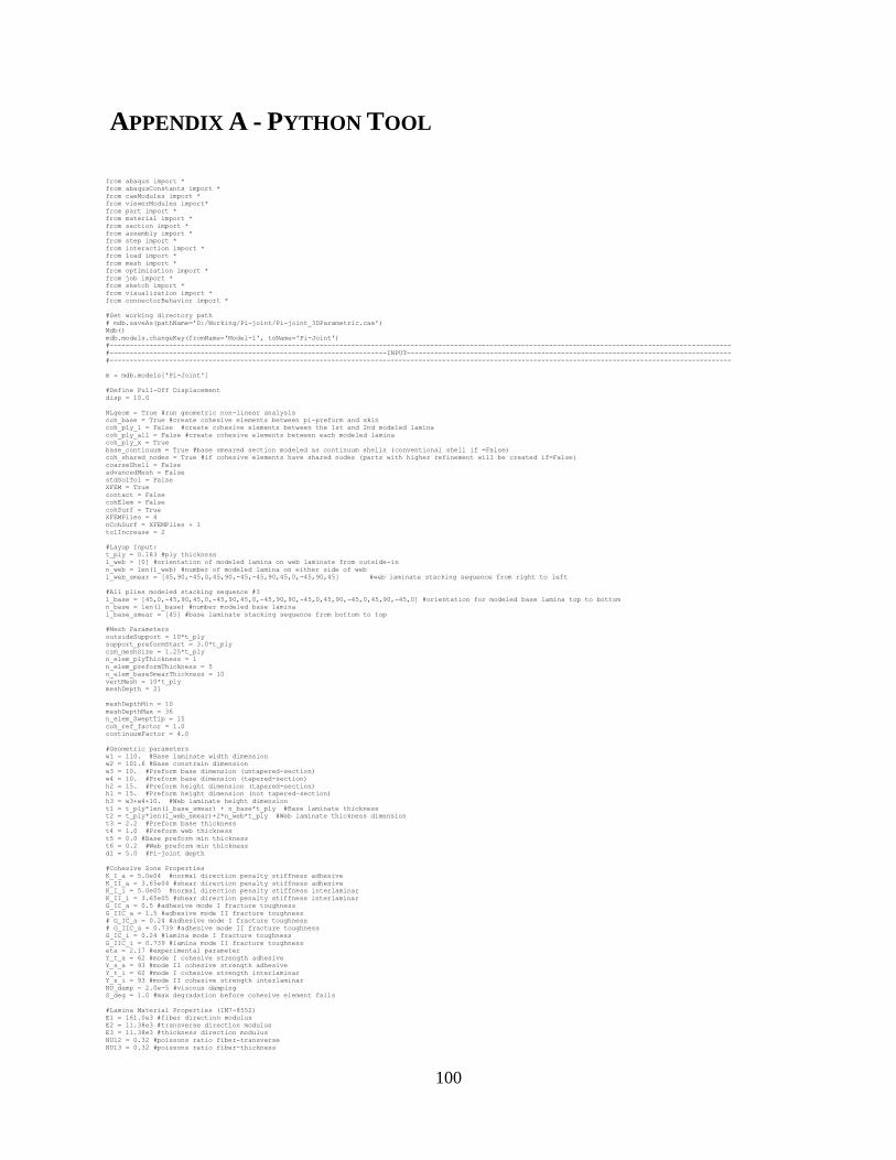
100

APPENDIX A - PYTHON TOOL

from abaqus import *

from abaqusConstants import *

from caeModules import *

from viewerModules import*

from part import *

from material import *

from section import *

from assembly import *

from step import *

from interaction import *

from load import *

from mesh import *

from optimization import *

from job import *

from sketch import *

from visualization import *

from connectorBehavior import *

#Set working directory path

# mdb.saveAs(pathName='D:/Working/Pi-joint/Pi-joint_3DParametric.cae')

Mdb()

mdb.models.changeKey(fromName='Model-1', toName='Pi-Joint')

#-------------------------------------------------------------------------------------------------------------------------------------------------------------

#----------------------------------------------------------------------INPUT----------------------------------------------------------------------------------

#-------------------------------------------------------------------------------------------------------------------------------------------------------------

m = mdb.models['Pi-Joint']

#Define Pull-Off Displacement

disp = 10.0

NLgeom = True #run geometric non-linear analysis

coh_base = True #create cohesive elements between pi-preform and skin

coh_ply_1 = False #create cohesive elements between the 1st and 2nd modeled lamina

coh_ply_all = False #create cohesive elements between each modeled lamina

coh_ply_x = True

base_continuum = True #base smeared section modeled as continuum shells (conventional shell if =False)

coh_shared_nodes = True #if cohesive elements have shared nodes (parts with higher refinement will be created if=False)

coarseShell = False

advancedMesh = False

stdSolTol = False

XFEM = True

contact = False

cohElem = False

cohSurf = True

XFEMPlies = 4

nCohSurf = XFEMPlies + 1

tolIncrease = 2

#Layup Input:

t_ply = 0.183 #ply thickness

l_web = [0] #orientation of modeled lamina on web laminate from outside-in

n_web = len(l_web) #number of modeled lamina on either side of web

l_web_smear = [45,90,-45,0,45,90,-45,-45,90,45,0,-45,90,45] #web laminate stacking sequence from right to left

#All plies modeled stacking sequence #3

l_base = [45,0,-45,90,45,0,-45,90,45,0,-45,90,90,-45,0,45,90,-45,0,45,90,-45,0] #orientation for modeled base lamina top to bottom

n_base = len(l_base) #number modeled base lamina

l_base_smear = [45] #base laminate stacking sequence from bottom to top

#Mesh Parameters

outsideSupport = 10*t_ply

support_preformStart = 3.0*t_ply

czm_meshSize = 1.25*t_ply

n_elem_plyThickness = 1

n_elem_preformThickness = 5

n_elem_baseSmearThickness = 10

vertMesh = 10*t_ply

meshDepth = 21

meshDepthMin = 10

meshDepthMax = 36

n_elem_SweptTip = 15

coh_ref_factor = 1.0

continuumFactor = 4.0

#Geometric parameters

w1 = 110. #Base laminate width dimension

w2 = 101.6 #Base constrain dimension

w3 = 10. #Preform base dimension (untapered-section)

w4 = 10. #Preform base dimension (tapered-section)

h2 = 15. #Preform height dimension (tapered-section)

h1 = 15. #Preform height dimension (not tapered-section)

h3 = w3+w4+10. #Web laminate height dimension

t1 = t_ply*len(l_base_smear) + n_base*t_ply #Base laminate thickness

t2 = t_ply*len(l_web_smear)+2*n_web*t_ply #Web laminate thickness dimension

t3 = 2.2 #Preform base thickness

t4 = 1.0 #Preform web thickness

t5 = 0.0 #Base preform min thickness

t6 = 0.2 #Web preform min thickness

d1 = 5.0 #Pi-joint depth

#Cohesive Zone Properties

K_I_a = 5.0e04 #normal direction penalty stiffness adhesive

K_II_a = 3.65e04 #shear direction penalty stiffness adhesive

K_I_i = 5.0e05 #normal direction penalty stiffness interlaminar

K_II_i = 3.65e05 #shear direction penalty stiffness interlaminar

G_IC_a = 0.5 #adhesive mode I fracture toughness

G_IIC_a = 1.5 #adhesive mode II fracture toughness

# G_IC_a = 0.24 #adhesive mode I fracture toughness

# G_IIC_a = 0.739 #adhesive mode II fracture toughness

G_IC_i = 0.24 #lamina mode I fracture toughness

G_IIC_i = 0.739 #lamina mode II fracture toughness

eta = 2.17 #experimental parameter

Y_t_a = 62 #mode I cohesive strength adhesive

Y_s_a = 93 #mode II cohesive strength adhesive

Y_t_i = 62 #mode I cohesive strength interlaminar

Y_s_i = 93 #mode II cohesive strength interlaminar

NU_damp = 2.0e-5 #viscous damping

S_deg = 1.0 #max degradation before cohesive element fails

#Lamina Material Properties (IM7-8552)

E1 = 161.0e3 #fiber direction modulus

E2 = 11.38e3 #transverse direction modulus

E3 = 11.38e3 #thickness direction modulus

NU12 = 0.32 #poissons ratio fiber-transverse

NU13 = 0.32 #poissons ratio fiber-thickness

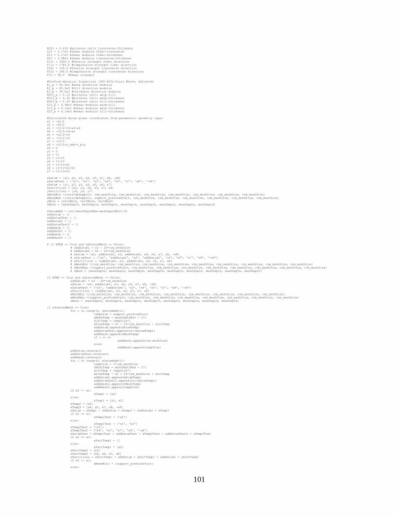
101

NU23 = 0.436 #poissons ratio transverse-thickness

G12 = 5.17e3 #shear modulus fiber-transverse

G13 = 5.17e3 #shear modulus fiber-thickness

G23 = 3.98e3 #shear modulus transverse-thickness

F11t = 2400.0 #Tensile strength fiber direction

F11c = 1785.0 #Compressive strength fiber direction

F22t = 100.0 #Tensile strength transverse direction

F22c = 290.0 #Compressive strength transverse direction

F12 = 98.0 #Shear strength

#Preform Material Properties (IM7-8552-Plain Weave, Adjusted)

E1_p = 65.0e3 #warp direction modulus

E2_p = 65.0e3 #fill direction modulus

E3_p = 30.0e3 #thickness direction modulus

NU12_p = 0.15 #poissons ratio warp-fill

NU13_p = 0.30 #poissons ratio warp-thickness

NU23_p = 0.30 #poissons ratio fill-thickness

G12_p = 4.48e3 #shear modulus warp-fill

G13_p = 4.14e3 #shear modulus warp-thickness

G23_p = 4.14e3 #shear modulus fill-thickness

#Calculated datum plane coordinates from parametric geometry input

x1 = -w1/2

x2 = -w2/2

x3 = -t2/2-t4-w3-w4

x4 = -t2/2-t4-w3

x5 = -t2/2-t4

x6 = -t2/2-t6

x7 = -t2/2

x8 = -t2/2+n_web*t_ply

x9 = 0

y1 = 0

y2 = t1

y3 = t1+t5

y4 = t1+t3

y5 = t1+t3+h1

y6 = t1+t3+h1+h2

y7 = t1+t3+h3

xDatum = [x1, x2, x3, x4, x5, x7, x8, -x8]

xDatumText = ['x1', 'x2', 'x3', 'x4', 'x5', 'x7', 'x8', '-x8']

yDatum = [y1, y2, y3, y4, y5, y6, y7]

xPartitions = [x2, x3, x4, x5, x7, x8]

yPartitions = [y4, y6, y7]

xMeshMin =[outsideSupport, czm_meshSize, czm_meshSize, czm_meshSize, czm_meshSize, czm_meshSize, czm_meshSize, czm_meshSize]

xMeshMax =[outsideSupport, support_preformStart, czm_meshSize, czm_meshSize, czm_meshSize, czm_meshSize, czm_meshSize, czm_meshSize]

yMesh = [vertMesh, vertMesh, vertMesh]

zMesh = [meshDepth, meshDepth, meshDepth, meshDepth, meshDepth, meshDepth, meshDepth, meshDepth]

nDatumAdd = int((meshDepthMax-meshDepthMin)/2)

addDatum = []

addDatumText = []

addDatum2 = []

addDatumText2 = []

addZmesh = []

addZmesh2 = []

addXmesh = []

addXmesh2 = []

# if XFEM == True and advancedMesh == False:

# addDatum1 = x3 - 20*czm_meshSize

# addDatum2 = x4 - 20*czm_meshSize

# xDatum = [x2, addDatum1, x3, addDatum2, x4, x5, x7, x8, -x8]

# xDatumText = ['x2', 'addDatum1', 'x3', 'addDatum2', 'x4', 'x5', 'x7', 'x8', '-x8']

# xPartitions = [addDatum1, x3, addDatum2, x4, x5, x7, x8]

# xMeshMin =[czm_meshSize, czm_meshSize, czm_meshSize, czm_meshSize, czm_meshSize, czm_meshSize, czm_meshSize, czm_meshSize, czm_meshSize]

# xMeshMax =[support_preformStart, czm_meshSize, czm_meshSize, czm_meshSize, czm_meshSize, czm_meshSize, czm_meshSize, czm_meshSize, czm_meshSize]

# zMesh = [meshDepth, meshDepth, meshDepth, meshDepth, meshDepth, meshDepth, meshDepth, meshDepth, meshDepth]

if XFEM == True and advancedMesh == False:

addDatum1 = x3 - 20*czm_meshSize

xDatum = [x2, addDatum1, x3, x4, x5, x7, x8, -x8]

xDatumText = ['x2', 'addDatum1', 'x3', 'x4', 'x5', 'x7', 'x8', '-x8']

xPartitions = [addDatum1, x3, x4, x5, x7, x8]

xMeshMin =[czm_meshSize, czm_meshSize, czm_meshSize, czm_meshSize, czm_meshSize, czm_meshSize, czm_meshSize, czm_meshSize]

xMeshMax =[support_preformStart, czm_meshSize, czm_meshSize, czm_meshSize, czm_meshSize, czm_meshSize, czm_meshSize, czm_meshSize]

zMesh = [meshDepth, meshDepth, meshDepth, meshDepth, meshDepth, meshDepth, meshDepth, meshDepth]

if advancedMesh == True:

for i in range(0, nDatumAdd+1):

tempSize = support_preformStart

zMeshTemp = meshDepthMin + 2*i

distTemp = tempSize*i

datumTemp = x3 - 25*czm_meshSize - distTemp

addDatum.append(datumTemp)

addDatumText.append(str(datumTemp))

addZmesh.append(zMeshTemp)

if i == 0:

addXmesh.append(czm_meshSize)

else:

addXmesh.append(tempSize)

addDatum.reverse()

addDatumText.reverse()

addXmesh.reverse()

for i in range(0, nDatumAdd+1):

tempSize = 3*czm_meshSize

zMeshTemp = meshDepthMax - 2*i

distTemp = tempSize*i

datumTemp = x3 + 25*czm_meshSize + distTemp

addDatum2.append(datumTemp)

addDatumText2.append(str(datumTemp))

addZmesh2.append(zMeshTemp)

addXmesh2.append(tempSize)

if w2 == w1:

xTemp1 = [x2]

else:

xTemp1 = [x1, x2]

xTemp2 = [x3]

xTemp3 = [x4, x5, x7, x8, -x8]

xDatum = xTemp1 + addDatum + xTemp2 + addDatum2 + xTemp3

if w2 == w1:

xTemp1Text = ['x2']

else:

xTemp1Text = ['x1', 'x2']

xTemp2Text = ['x3']

xTemp3Text = ['x4', 'x5', 'x7', 'x8', '-x8']

xDatumText = xTemp1Text + addDatumText + xTemp2Text + addDatumText2 + xTemp3Text

if w2 == w1:

xPartTemp1 = []

else:

xPartTemp1 = [x2]

xPartTemp2 = [x3]

xPartTemp3 = [x4, x5, x7, x8]

xPartitions = xPartTemp1 + addDatum + xPartTemp2 + addDatum2 + xPartTemp3

if w2 == w1:

xMeshMin1 = [support_preformStart]

else:

102

xMeshMin1 = [outsideSupport, support_preformStart]

xMeshMin2 = [czm_meshSize]

xMeshMin3 = [3*czm_meshSize, 3*czm_meshSize, 3*czm_meshSize, 3*czm_meshSize, 3*czm_meshSize, 3*czm_meshSize]

xMeshMin = xMeshMin1 + addXmesh + xMeshMin2 + addXmesh2 + xMeshMin3

xMeshMax = xMeshMin

if w2 == w1:

zMesh1 = [meshDepthMin]

else:

zMesh1 = [meshDepthMin, meshDepthMin]

zMesh2 = [meshDepthMax]

zMesh3 = [meshDepthMin, meshDepthMin, meshDepthMin, meshDepthMin, meshDepthMin]

zMesh = zMesh1 + addZmesh + zMesh2 + addZmesh2 + zMesh3

print len(xDatum)

print len(xMeshMin)

print zMesh1

print addZmesh

print zMesh2

print addZmesh2

print zMesh3

print zMesh

if w2 == w1 and advancedMesh == False and XFEM == False:

xDatum = [x2, x3, x4, x5, x7, x8, -x8]

xDatumText = ['x2', 'x3', 'x4', 'x5', 'x7', 'x8', '-x8']

xPartitions = [x3, x4, x5, x7, x8]

xMeshMin =[czm_meshSize, czm_meshSize, czm_meshSize, czm_meshSize, czm_meshSize, czm_meshSize, czm_meshSize, czm_meshSize]

xMeshMax =[support_preformStart, czm_meshSize, czm_meshSize, czm_meshSize, czm_meshSize, czm_meshSize, czm_meshSize, czm_meshSize]

if t5==0:

addDatum = x3 + n_elem_SweptTip*xMeshMin[2]

xDatum = [x1, x2, x3, addDatum, x4, x5, x7, x8, -x8]

xDatumText = ['x1', 'x2', 'x3', 'addDatum', 'x4', 'x5', 'x7', 'x8', '-x8']

xPartitions = [x2, x3, addDatum, x4, x5, x7, x8]

xMeshMin =[outsideSupport, czm_meshSize, czm_meshSize, czm_meshSize, czm_meshSize, czm_meshSize, czm_meshSize, czm_meshSize, czm_meshSize]

xMeshMax =[outsideSupport, support_preformStart, czm_meshSize, czm_meshSize, czm_meshSize, czm_meshSize, czm_meshSize, czm_meshSize, czm_meshSize]

for i in range(0,len(xDatum)-1):

if xDatumText[i] == 'x7':

pos_x7 = i


pos_x8 = i


pos_x3 = i


pos_x4 = i


pos_x5 = i

if xDatumText[i] == 'addDatum':

pos_addDatum = i

SeedNumber = [0]*len(xDatum)

for j in range(1, len(xDatum)):

if j >= pos_x3+1:

xmin = xDatum[j-1]

xmax = xDatum[j]

SeedNumber[j] = int(abs(round((xmin-xmax)/xMeshMin[j-1],0)))

if SeedNumber[j] == 0:

SeedNumber[j] = SeedNumber[j] + 1

if SeedNumber[j] > 1 and coh_shared_nodes == False:

while SeedNumber[j]%coh_ref_factor != 0:

SeedNumber[j] = SeedNumber[j] + 1

print SeedNumber

SeedNumberCoh = [0]*len(xDatum)


if j < pos_x3+1:

SeedNumberCoh[j] = SeedNumber[j]

else:

SeedNumberCoh[j] = int(SeedNumber[j]*coh_ref_factor)

print SeedNumberCoh

if coh_shared_nodes == False and meshDepth%coh_ref_factor != 0:

while meshDepth%coh_ref_factor != 0:

meshDepth = meshDepth + 1

#-------------------------------------------------------------------------------------------------------------------------------------------------------------

#------------------------------------------------------------------GENERATE MATERIALS-------------------------------------------------------------------------

#-------------------------------------------------------------------------------------------------------------------------------------------------------------

#Lamina Material

m.Material(name='IM7-8552')

m.materials['IM7-8552'].Elastic(

type=ENGINEERING_CONSTANTS,

table=((E1, E2, E3, NU12, NU13, NU23, G12, G13, G23), ))

m.materials['IM7-8552'].elastic.FailStress(

table=((F11t, F11c, F22t, F22c, F12, 0.0, 0.0), ))

#Lamina XFEM Material LARCO5 Built-in Subroutine

m.Material(name='ABQ_LARC05_DMGINI_IM7-8552-Xfem')

m.materials['ABQ_LARC05_DMGINI_IM7-8552-Xfem'].Elastic(


table=((E1, E2, E3, NU12, NU13, NU23, G12, G13, G23), ))

# *Material, name=ABQ_LARC05_DMGINI_IM7-8552-Xfem

# *Depvar, delete=16

# 16,

# *Elastic, type=ENGINEERING CONSTANTS

# 161000.,11380.,11380., 0.32, 0.32, 0.436, 5170., 5170.

# 3980.,

# *DAMAGE INITIATION, CRITERION=USER, FAILURE MECHANISMS=4,PROPERTIES=15,tol=0.1

# 161000., 11380., 0.32, 0.436, 5170., 2400.0, 1785.0, 100.0

# 290.0, 98.0, 53., 2.544, 101., 0.082, 0.29,

# *DAMAGE EVOLUTION,FAILURE INDEX=1,TYPE=ENERGY, mixed mode behavior=BK, power=2.17

# 0.24, 0.739, 0.739

# *DAMAGE EVOLUTION,FAILURE INDEX=2,TYPE=ENERGY

# 106.3


# 50.


# 97.8

# *DAMAGE STABILIZATION

# 1.e-4

#Preform Material

m.Material(name='IM7-8552-W')

m.materials['IM7-8552-W'].Elastic(


table=((E1_p, E2_p, E3_p, NU12_p, NU13_p, NU23_p, G12_p, G13_p, G23_p), ))

#Cohesive property-adhesive (pi-preform and skin)

m.Material(name='pi-skin-prop')

m.materials['pi-skin-prop'].Elastic(table=((K_I_a, K_II_a, K_II_a), ), type=TRACTION)

m.materials['pi-skin-prop'].QuadsDamageInitiation(table=((Y_t_a, Y_s_a, Y_s_a), ))

m.materials['pi-skin-prop'].quadsDamageInitiation.DamageEvolution(

mixedModeBehavior=BK, power=eta, table=((G_IC_a, G_IIC_a, G_IIC_a), ), type=ENERGY)

m.materials['pi-skin-prop'].quadsDamageInitiation.DamageStabilizationCohesive(cohesiveCoeff=NU_damp)

#Cohesive property-lamina (interlamianar)

m.Material(name='interlaminar-prop')

m.materials['interlaminar-prop'].Elastic(table=((K_I_i, K_II_i, K_II_i), ), type=TRACTION)

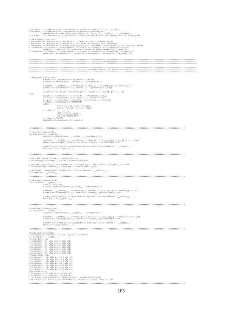
103

m.materials['interlaminar-prop'].QuadsDamageInitiation(table=((Y_t_i, Y_s_i, Y_s_i), ))

m.materials['interlaminar-prop'].quadsDamageInitiation.DamageEvolution(

mixedModeBehavior=BK, power=eta, table=((G_IC_i, G_IIC_i, G_IIC_i), ), type=ENERGY)

m.materials['interlaminar-prop'].quadsDamageInitiation.DamageStabilizationCohesive(cohesiveCoeff=NU_damp)

#Create property sections

m.HomogeneousSolidSection(material='IM7-8552', name='IM7-8552', thickness=None)

m.HomogeneousSolidSection(material='IM7-8552-W', name='IM7-8552-W', thickness=None)

m.HomogeneousSolidSection(material='ABQ_LARC05_DMGINI_IM7-8552-Xfem', name='IM7-8552-Xfem', thickness=None)

m.CohesiveSection(initialThicknessType=SPECIFY, initialThickness=1.0, material='pi-skin-prop',

name='pi-skin-section', outOfPlaneThickness=None, response=TRACTION_SEPARATION)

m.CohesiveSection(initialThicknessType=SPECIFY, initialThickness=1.0, material='interlaminar-prop',

name='interlaminar-section', outOfPlaneThickness=None, response=TRACTION_SEPARATION)

#-------------------------------------------------------------------------------------------------------------------------------------------------------------

#--------------------------------------------------------------------END MATERIALS----------------------------------------------------------------------------

#-------------------------------------------------------------------------------------------------------------------------------------------------------------

#-------------------------------------------------------------------------------------------------------------------------------------------------------------

#-------------------------------------------------------GENERATE GEOMETRY AND ASSIGN SECTION------------------------------------------------------------------

#-------------------------------------------------------------------------------------------------------------------------------------------------------------

if base_continuum == True:

#Create Base Laminate Geometry (smeared section)

m.ConstrainedSketch(name='__profile__', sheetSize=200.0)

m.sketches['__profile__'].rectangle(point1=(x1, y2 - n_base*t_ply), point2=(-x1, y1))

m.Part(dimensionality=THREE_D, name='Base', type=DEFORMABLE_BODY)

m.parts['Base'].BaseSolidExtrude(depth=d1, sketch=m.sketches['__profile__'])

else:

#Create Base-Smear Laminate as 2D Shell (CONVENTIONAL_SHELL)

s = m.ConstrainedSketch(name='__profile__', sheetSize=200)

g, v, d, c = s.geometry, s.vertices, s.dimensions, s.constraints

s.setPrimaryObject(option=STANDALONE)

s.Line(

point1=(x1, y2 - n_base*t_ply),

point2=(-x1, y2 - n_base*t_ply))

p = m.Part(

name='Base',

dimensionality=THREE_D,

type=DEFORMABLE_BODY)

p = m.parts['Base']

p.BaseShellExtrude(depth=d1, sketch=s)

##################################################################################################################################################

#Create Base Modeled Plies

for i in range(1, n_base+1, 1):


m.sketches['__profile__'].rectangle(point1=(x1, y2-i*t_ply), point2=(-x1, y2-(i-1)*t_ply))

m.Part(dimensionality=THREE_D, name='Base-'+str(i), type=DEFORMABLE_BODY)

m.parts['Base-'+str(i)].BaseSolidExtrude(depth=d1, sketch=m.sketches['__profile__'])

del m.sketches['__profile__']

##################################################################################################################################################

#Create Web Laminate Geometry (smeared section)


m.sketches['__profile__'].rectangle(point1=(x7+n_web*t_ply, y4), point2=(-x7-n_web*t_ply, y7))

m.Part(dimensionality=THREE_D, name='Web', type=DEFORMABLE_BODY)

m.parts['Web'].BaseSolidExtrude(depth=d1, sketch=m.sketches['__profile__'])


##################################################################################################################################################

#Create Web-L Modeled Plies

for i in range(1, n_web+1, 1):

theta = l_web[i-1]


m.sketches['__profile__'].rectangle(point1=(x7+(i-1)*t_ply, y4), point2=(x7+i*t_ply, y7))

m.Part(dimensionality=THREE_D, name='Web-L'+str(i), type=DEFORMABLE_BODY)

m.parts['Web-L'+str(i)].BaseSolidExtrude(depth=d1, sketch=m.sketches['__profile__'])


##################################################################################################################################################

#Create Web-R Modeled Plies



m.sketches['__profile__'].rectangle(point1=(-x7-(i-1)*t_ply, y4), point2=(-x7-i*t_ply, y7))

m.Part(dimensionality=THREE_D, name='Web-R'+str(i), type=DEFORMABLE_BODY)

m.parts['Web-R'+str(i)].BaseSolidExtrude(depth=d1, sketch=m.sketches['__profile__'])


##################################################################################################################################################

#Create Preform Geometry


s = m.sketches['__profile__']

#Preform Left-side

s.Line(point1=(x3, y2), point2=(x3, y3))







#Preform Right-side

s.Line(point1=(-x3, y2), point2=(-x3, y3))







#Connecting Lines

s.Line(point1=(x7, y4), point2=(-x7, y4))

s.Line(point1=(x3, y2), point2=(-x3, y2))

m.Part(dimensionality=THREE_D, name='Preform', type=DEFORMABLE_BODY)

m.parts['Preform'].BaseSolidExtrude(depth=d1, sketch=m.sketches['__profile__'])

##################################################################################################################################################

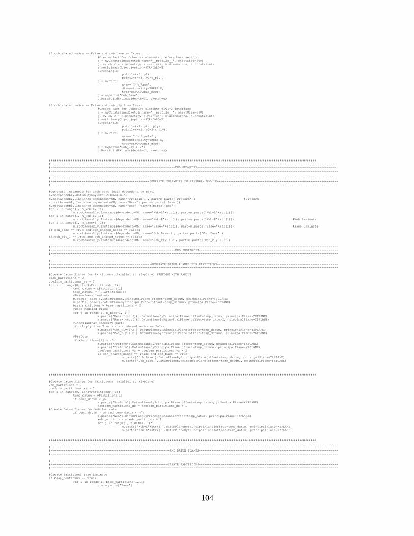
104

if coh_shared_nodes == False and coh_base == True:

#Create Part for Cohesive elements preform base section




s.rectangle(

point1=(x3, y2),

point2=(-x3, y2-t_ply))

p = m.Part(

name='Coh_Base',



p = m.parts['Coh_Base']

p.BaseSolidExtrude(depth=d1, sketch=s)

if coh_shared_nodes == False and coh_ply_1 == True:

#Create Part for Cohesive elements ply1-2 interface




s.rectangle(

point1=(x1, y2-t_ply),

point2=(-x1, y2-2*t_ply))

p = m.Part(

name='Coh_Ply-1-2',



p = m.parts['Coh_Ply-1-2']

p.BaseSolidExtrude(depth=d1, sketch=s)

##################################################################################################################################################

#-------------------------------------------------------------------------------------------------------------------------------------------------------------

#--------------------------------------------------------------------END GEOMETRY----------------------------------------------------------------------------

#-------------------------------------------------------------------------------------------------------------------------------------------------------------

#-------------------------------------------------------------------------------------------------------------------------------------------------------------

#------------------------------------------------------GENERATE INSTANCES IN ASSEMBLY MODULE------------------------------------------------------------------

#-------------------------------------------------------------------------------------------------------------------------------------------------------------

#Generate Instances for each part (mesh dependent on part)

m.rootAssembly.DatumCsysByDefault(CARTESIAN)

m.rootAssembly.Instance(dependent=ON, name='Preform-1', part=m.parts['Preform']) #Preform

m.rootAssembly.Instance(dependent=ON, name='Base', part=m.parts['Base'])

m.rootAssembly.Instance(dependent=ON, name='Web', part=m.parts['Web'])


m.rootAssembly.Instance(dependent=ON, name='Web-L'+str(i), part=m.parts['Web-L'+str(i)])


m.rootAssembly.Instance(dependent=ON, name='Web-R'+str(i), part=m.parts['Web-R'+str(i)]) #Web laminate


m.rootAssembly.Instance(dependent=ON, name='Base-'+str(i), part=m.parts['Base-'+str(i)]) #Base laminate

if coh_base == True and coh_shared_nodes == False:

m.rootAssembly.Instance(dependent=ON, name='Coh_Base-1', part=m.parts['Coh_Base'])

if coh_ply_1 == True and coh_shared_nodes == False:

m.rootAssembly.Instance(dependent=ON, name='Coh_Ply-1-2', part=m.parts['Coh_Ply-1-2'])

#-------------------------------------------------------------------------------------------------------------------------------------------------------------

#--------------------------------------------------------------------END INSTANCES----------------------------------------------------------------------------

#-------------------------------------------------------------------------------------------------------------------------------------------------------------

#-------------------------------------------------------------------------------------------------------------------------------------------------------------

#-------------------------------------------------------GENERATE DATUM PLANES FOR PARTITIONS------------------------------------------------------------------

#-------------------------------------------------------------------------------------------------------------------------------------------------------------

#Create Datum Planes for Partitions (Parallel to YZ-plane) PREFORM WITH RADIUS

base_partitions = 0

preform_partitions_yz = 0

for i in range(0, len(xPartitions), 1):

temp_datum = xPartitions[i]

temp_datum2 = -xPartitions[i]

#Base-Smear Laminate

m.parts['Base'].DatumPlaneByPrincipalPlane(offset=temp_datum, principalPlane=YZPLANE)

m.parts['Base'].DatumPlaneByPrincipalPlane(offset=temp_datum2, principalPlane=YZPLANE)

base_partitions = base_partitions + 2

#Base-Modeled Plies

for j in range(1, n_base+1, 1):

m.parts['Base-'+str(j)].DatumPlaneByPrincipalPlane(offset=temp_datum, principalPlane=YZPLANE)

m.parts['Base-'+str(j)].DatumPlaneByPrincipalPlane(offset=temp_datum2, principalPlane=YZPLANE)

#Interlaminar cohesive parts


m.parts['Coh_Ply-1-2'].DatumPlaneByPrincipalPlane(offset=temp_datum, principalPlane=YZPLANE)

m.parts['Coh_Ply-1-2'].DatumPlaneByPrincipalPlane(offset=temp_datum2, principalPlane=YZPLANE)

#Preform

if xPartitions[i] > x3:

m.parts['Preform'].DatumPlaneByPrincipalPlane(offset=temp_datum, principalPlane=YZPLANE)

m.parts['Preform'].DatumPlaneByPrincipalPlane(offset=temp_datum2, principalPlane=YZPLANE)

preform_partitions_yz = preform_partitions_yz + 2


m.parts['Coh_Base'].DatumPlaneByPrincipalPlane(offset=temp_datum, principalPlane=YZPLANE)

m.parts['Coh_Base'].DatumPlaneByPrincipalPlane(offset=temp_datum2, principalPlane=YZPLANE)

##################################################################################################################################################

#Create Datum Planes for Partitions (Parallel to XZ-plane)

web_partitions = 0

preform_partitions_xz = 0

for i in range(0, len(yPartitions), 1):

temp_datum = yPartitions[i]

if temp_datum < y6:

m.parts['Preform'].DatumPlaneByPrincipalPlane(offset=temp_datum, principalPlane=XZPLANE)

preform_partitions_xz = preform_partitions_xz + 1

#Create Datum Planes for Web Laminate

if temp_datum > y4 and temp_datum < y7:

m.parts['Web'].DatumPlaneByPrincipalPlane(offset=temp_datum, principalPlane=XZPLANE)

web_partitions = web_partitions + 1

for j in range(1, n_web+1, 1):

m.parts['Web-L'+str(j)].DatumPlaneByPrincipalPlane(offset=temp_datum, principalPlane=XZPLANE)

m.parts['Web-R'+str(j)].DatumPlaneByPrincipalPlane(offset=temp_datum, principalPlane=XZPLANE)

##################################################################################################################################################

#-------------------------------------------------------------------------------------------------------------------------------------------------------------

#-----------------------------------------------------------------END DATUM PLANES----------------------------------------------------------------------------

#-------------------------------------------------------------------------------------------------------------------------------------------------------------

#-------------------------------------------------------------------------------------------------------------------------------------------------------------

#----------------------------------------------------------------CREATE PARTITIONS----------------------------------------------------------------------------

#-------------------------------------------------------------------------------------------------------------------------------------------------------------

#Create Partitions Base Laminate


for i in range(1, base_partitions+1,1):

p = m.parts['Base']

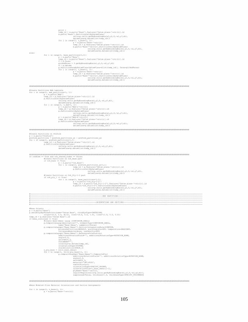
105

print i

temp_id = m.parts['Base'].features['Datum plane-'+str(i)].id

m.parts['Base'].PartitionCellByDatumPlane(

cells=p.cells.getByBoundingBox(x1,y1,0,-x1,y7,d1),

datumPlane=p.datums[int(temp_id)])


p = m.parts['Base-'+str(j)]

temp_id = p.features['Datum plane-'+str(i)].id

m.parts['Base-'+str(j)].PartitionCellByDatumPlane(



else:


p = m.parts['Base']

temp_id = m.parts['Base'].features['Datum plane-'+str(i)].id

f = p.faces

pickedFaces = f.getByBoundingBox(x1,y1,0,-x1,y7,d1)

d = p.datums

p.PartitionFaceByDatumPlane(datumPlane=d[int(temp_id)], faces=pickedFaces)


p = m.parts['Base-'+str(j)]


m.parts['Base-'+str(j)].PartitionCellByDatumPlane(



##################################################################################################################################################

#Create Partitions Web Laminate

for i in range(1, web_partitions+1, 1):

p = m.parts['Web']


p.PartitionCellByDatumPlane(



for j in range(1, n_web+1, 1):

p = m.parts['Web-L'+str(j)]





p = m.parts['Web-R'+str(j)]





##################################################################################################################################################

#Create Partitions on Preform

p = m.parts['Preform']

preform_partitions = preform_partitions_yz + preform_partitions_xz

for i in range(1, preform_partitions+1,):





##################################################################################################################################################

if cohElem == True and coh_shared_nodes == False:

#Create Partitions on Coh_Base part

if coh_base == True:


for i in range(1, preform_partitions_yz+1,):





#Create Partitions on Coh_Ply-1-2 part

if coh_ply_1 == True:



temp_id = m.parts['Coh_Ply-1-2'].features['Datum plane-'+str(i)].id

m.parts['Coh_Ply-1-2'].PartitionCellByDatumPlane(



#-------------------------------------------------------------------------------------------------------------------------------------------------------------

#------------------------------------------------------------------END PARTITIONS-----------------------------------------------------------------------------

#-------------------------------------------------------------------------------------------------------------------------------------------------------------

#-------------------------------------------------------------------------------------------------------------------------------------------------------------

#------------------------------------------------------------ORIENTATIONS AND SECTIONS------------------------------------------------------------------------

#-------------------------------------------------------------------------------------------------------------------------------------------------------------

#Base Orients

p = m.parts['Base']

p.DatumCsysByThreePoints(name='Datum Base', coordSysType=CARTESIAN,

origin=(0.0, 0.0, d1/2), line1=(0.0, 0.0, 1.0), line2=(1.0, 0.0, 0.0))

temp_id = p.features['Datum Base'].id


#Create Base-Smear Layup (CONTINUUM_SHELL)

p.CompositeLayup(description='', elementType=CONTINUUM_SHELL,

name='Base-Smear', symmetric=False)

p.compositeLayups['Base-Smear'].Section(integrationRule=SIMPSON,

poissonDefinition=DEFAULT, preIntegrate=OFF, temperature=GRADIENT,

thicknessModulus=None, useDensity=OFF)

p.compositeLayups['Base-Smear'].ReferenceOrientation(

additionalRotationField='', additionalRotationType=ROTATION_NONE,

angle=0.0,

axis=AXIS_3,

fieldName='',

localCsys=p.datums[temp_id],

orientationType=SYSTEM,

stackDirection=STACK_3)

n_ply_base = len(l_base_smear)

for i in range(1, int(n_ply_base)+1, 1):

p.compositeLayups['Base-Smear'].CompositePly(


angle=0.0,

axis=AXIS_3,

material='IM7-8552',

numIntPoints=3,

orientationType=SPECIFY_ORIENT,

orientationValue=l_base_smear[i-1],

plyName='Base-'+str(i),

region=Region(cells=p.cells.getByBoundingBox(x1,y1,0,-x1,y2,d1)),

suppressed=False, thickness=1.0, thicknessType=SPECIFY_THICKNESS)

##################################################################################################################################################

#Base Modeled Plies Material Orientations and Section Assignments


p = m.parts['Base-'+str(i)]

106

theta = l_base[i-1]

p.DatumCsysByThreePoints(

name='Datum Base-'+str(i),

coordSysType=CARTESIAN,

origin=(0.0, y2-i*t_ply, d1/2),

line1=(0.0, 0.0, 1.0),

line2=(1.0, 0.0, 0.0))

temp_id = p.features['Datum Base-'+str(i)].id

p.MaterialOrientation(

additionalRotationField='', additionalRotationType=ROTATION_ANGLE,

angle=theta,

axis=AXIS_3,

fieldName='',



region=Region(cells=p.cells.getByBoundingBox(x1,y2-i*t_ply,0,-x1,y2-(i-1)*t_ply,d1)),


# if XFEM == True and i < XFEMPlies+1:

# if advancedMesh == False:

# cellOne = p.cells.getByBoundingBox(x1,y2-i*t_ply,0,addDatum1,y2-(i-1)*t_ply,d1)

# cellTwo = p.cells.getByBoundingBox(addDatum2,y2-i*t_ply,0,-addDatum2,y2-(i-1)*t_ply,d1)

# cellThree = p.cells.getByBoundingBox(-addDatum1,y2-i*t_ply,0,-x1,y2-(i-1)*t_ply,d1)

# else:

# cellOne = p.cells.getByBoundingBox(x1,y2-i*t_ply,0,addDatum[len(addDatum)-1],y2-(i-1)*t_ply,d1)

# cellTwo = p.cells.getByBoundingBox(addDatum2[0],y2-i*t_ply,0,-addDatum2[0],y2-(i-1)*t_ply,d1)

# cellThree = p.cells.getByBoundingBox(-addDatum[len(addDatum)-1],y2-i*t_ply,0,-x1,y2-(i-1)*t_ply,d1)

# cells = cellOne + cellTwo + cellThree

# p.SectionAssignment(

# offset=0.0, offsetField='', offsetType=MIDDLE_SURFACE,

# region=Region(cells=cells),

# sectionName='IM7-8552',

# thicknessAssignment=FROM_SECTION)


# cellOne = p.cells.getByBoundingBox(addDatum1,y2-i*t_ply,0,addDatum2,y2-(i-1)*t_ply,d1)

# cellTwo = p.cells.getByBoundingBox(-addDatum2,y2-i*t_ply,0,-addDatum1,y2-(i-1)*t_ply,d1)

# else:

# cellOne = p.cells.getByBoundingBox(addDatum[len(addDatum)-1],y2-i*t_ply,0,addDatum2[0],y2-(i-1)*t_ply,d1)

# cellTwo = p.cells.getByBoundingBox(-addDatum2[0],y2-i*t_ply,0,-addDatum[len(addDatum)-1],y2-(i-1)*t_ply,d1)

# cells = cellOne + cellTwo



# region=Region(cells=cells),

# sectionName='IM7-8552-Xfem',

# thicknessAssignment=FROM_SECTION)

# else:



# region=Region(cells=p.cells.getByBoundingBox(x1,y2-i*t_ply,0,-x1,y2-(i-1)*t_ply,d1)),

# sectionName='IM7-8552', thicknessAssignment=FROM_SECTION)

if XFEM == True and i < XFEMPlies+1:

if advancedMesh == False:

cellOne = p.cells.getByBoundingBox(x1,y2-i*t_ply,0,addDatum1,y2-(i-1)*t_ply,d1)

cellTwo = p.cells.getByBoundingBox(-addDatum1,y2-i*t_ply,0,-x1,y2-(i-1)*t_ply,d1)

cells = cellOne + cellTwo

p.SectionAssignment(

offset=0.0, offsetField='', offsetType=MIDDLE_SURFACE,

region=Region(cells=cells),

sectionName='IM7-8552',

thicknessAssignment=FROM_SECTION)


cellOne = p.cells.getByBoundingBox(addDatum1,y2-i*t_ply,0,-addDatum1,y2-(i-1)*t_ply,d1)

cells = cellOne



region=Region(cells=cells),

sectionName='IM7-8552-Xfem',


else:



region=Region(cells=p.cells.getByBoundingBox(x1,y2-i*t_ply,0,-x1,y2-(i-1)*t_ply,d1)),

sectionName='IM7-8552', thicknessAssignment=FROM_SECTION)

##################################################################################################################################################

#Web-Smear Layup (CONTINUUM_SHELL)

p = m.parts['Web']

p.DatumCsysByThreePoints(name='Datum Web', coordSysType=CARTESIAN,

origin=(0.0, (y4+y7)/2, d1/2), line1=(0.0, 0.0, 1.0), line2=(0.0, 1.0, 0.0))

temp_id = p.features['Datum Web'].id

p.CompositeLayup(description='', elementType=CONTINUUM_SHELL,

name='Web-Smear', symmetric=False)

p.compositeLayups['Web-Smear'].Section(integrationRule=SIMPSON,

poissonDefinition=DEFAULT, preIntegrate=OFF, temperature=GRADIENT,

thicknessModulus=None, useDensity=OFF)

p.compositeLayups['Web-Smear'].ReferenceOrientation(


angle=0.0,

axis=AXIS_3,

fieldName='',




n_ply_web = len(l_web_smear)

for i in range(1, int(n_ply_web)+1, 1):

p.compositeLayups['Web-Smear'].CompositePly(


angle=0.0,

axis=AXIS_3,

material='IM7-8552',

numIntPoints=3,

orientationType=SPECIFY_ORIENT,

orientationValue=l_web_smear[i-1],

plyName='Web-'+str(i),

region=Region(cells=p.cells.getByBoundingBox(x7+n_web*t_ply,y4,0,-x7-n_web*t_ply,y7,d1)),

suppressed=False, thickness=1.0, thicknessType=SPECIFY_THICKNESS)

##################################################################################################################################################

#Web-L Material Orientations and Section Assignments


p = m.parts['Web-L'+str(i)]

theta = l_web[i-1]


name='Datum Web-L'+str(i),


origin=(x7+i*t_ply,(y4+y7)/2, d1/2),

line1=(0.0, 0.0, 1.0), line2=(0.0, 1.0, 0.0))

temp_id = p.features['Datum Web-L'+str(i)].id



angle=theta,

axis=AXIS_3,

fieldName='',



107

region=Region(cells=p.cells.getByBoundingBox(x7+(i-1)*t_ply,y4,0,x7+i*t_ply,y7,d1)),




region=Region(cells=p.cells.getByBoundingBox(x7+(i-1)*t_ply,y4,0,x7+i*t_ply,y7,d1)),


##################################################################################################################################################

#Web-R Material Orientations and Section Assignments


p = m.parts['Web-R'+str(i)]

theta = l_web[i-1]


name='Datum Web-R'+str(i), coordSysType=CARTESIAN,

origin=(-x7-(i-1)*t_ply,(y4+y7)/2, d1/2),

line1=(0.0, 0.0, 1.0), line2=(0.0, 1.0, 0.0))

temp_id = p.features['Datum Web-R'+str(i)].id



angle=theta,

axis=AXIS_3,

fieldName='',



region=Region(cells=p.cells.getByBoundingBox(-x7-i*t_ply,y4,0,-x7-(i-1)*t_ply,y7,d1)),




region=Region(cells=p.cells.getByBoundingBox(-x7-i*t_ply,y4,0,-x7-(i-1)*t_ply,y7,d1)),


##################################################################################################################################################

#Preform Material Orientations and Section Assignments


c = p.cells

f = p.faces

e = p.edges

#Base


name='Datum Preform-Base', coordSysType=CARTESIAN,

origin=(0.0, (y2+y4)/2, d1/2),

line1=(0.0, 0.0, 1.0), line2=(1.0, 0.0, 0.0))

temp_id = p.features['Datum Preform-Base'].id

m.parts['Preform'].MaterialOrientation(


angle=0.0,

axis=AXIS_3,

fieldName='',



region=Region(cells=p.cells.getByBoundingBox(x3,y2,0,-x3,y4,d1)),


#Left Flange


name='Datum Preform-FL',


origin=((x5+x7)/2, (y4+y6)/2, d1/2),

line1=(0.0, 0.0, 1.0), line2=(0.0, 1.0, 0.0))

temp_id = p.features['Datum Preform-FL'].id



angle=0.0,

axis=AXIS_3,

fieldName='',



region=Region(cells=p.cells.getByBoundingBox(x5,y4,0,x7,y7,d1)),


#Right Flange


name='Datum Preform-FR', coordSysType=CARTESIAN,

origin=(-(x5+x7)/2, (y4+y6)/2, d1/2),

line1=(0.0, 0.0, 1.0), line2=(0.0, 1.0, 0.0))

temp_id = p.features['Datum Preform-FR'].id



angle=0.0,

axis=AXIS_3,

fieldName='',



region=Region(cells=p.cells.getByBoundingBox(-x7,y4,0,-x5,y7,d1)),




region=Region(cells=m.parts['Preform'].cells.getByBoundingBox(x1,y1,0,-x1,y7,d1)),

sectionName='IM7-8552-W', thicknessAssignment=FROM_SECTION)

#-------------------------------------------------------------------------------------------------------------------------------------------------------------

#------------------------------------------------------------END ORIENTATIONS AND SECTIONS--------------------------------------------------------------------

#-------------------------------------------------------------------------------------------------------------------------------------------------------------

#-------------------------------------------------------------------------------------------------------------------------------------------------------------

#--------------------------------------------------------------------SEED PARTS-------------------------------------------------------------------------------

#-------------------------------------------------------------------------------------------------------------------------------------------------------------

#Seed Parts

part_array = ['Base','Web','Preform']

for i in range(1, len(part_array)+1, 1):

m.parts[str(part_array[i-1])].seedPart(deviationFactor=0.01, minSizeFactor=0.1, size=support_preformStart*10)

for i in range(1, n_base+1,1):

m.parts['Base-'+str(i)].seedPart(deviationFactor=0.1, minSizeFactor=0.1, size=support_preformStart*10)

for i in range(1, n_web+1,1):

m.parts['Web-L'+str(i)].seedPart(deviationFactor=0.1, minSizeFactor=0.1, size=support_preformStart*10)

m.parts['Web-R'+str(i)].seedPart(deviationFactor=0.1, minSizeFactor=0.1, size=support_preformStart*10)


m.parts['Coh_Base'].seedPart(deviationFactor=0.01, minSizeFactor=0.1, size=support_preformStart*10)

#-------------------------------------------------------------------------------------------------------------------------------------------------------------

#------------------------------------------------------------------END SEED PARTS-----------------------------------------------------------------------------

#-------------------------------------------------------------------------------------------------------------------------------------------------------------

#-------------------------------------------------------------------------------------------------------------------------------------------------------------

#-------------------------------------------------------------------SEED EDGES--------------------------------------------------------------------------------

#-------------------------------------------------------------------------------------------------------------------------------------------------------------

#Seed edges for modeled base plies and smear base laminate

for i in range(1, n_base+1):


xmin = xDatum[j-1]

xmax = xDatum[j]

minSize_temp = xMeshMin[j-1]

maxSize_temp = xMeshMax[j-1]


e = p.edges

108

#Global X-direction (left of orgin, upper edges)

edges = e.findAt((((xmin+xmax)/2, y2-(i-1)*t_ply, d1), ),(((xmin+xmax)/2, y2-(i-1)*t_ply, 0), ),)

if j < pos_x4:

p.seedEdgeByBias(

biasMethod=SINGLE,

constraint=FINER,

end2Edges=edges,

maxSize=maxSize_temp,

minSize=minSize_temp)

else:

p.seedEdgeByNumber(

constraint=FINER,

edges=edges,

number=SeedNumber[j])

#Global X-direction (right of orgin, upper edges)

edges = e.findAt(((-(xmin+xmax)/2, y2-(i-1)*t_ply, d1), ),((-(xmin+xmax)/2, y2-(i-1)*t_ply, 0), ))

if j < pos_x4:

p.seedEdgeByBias(

biasMethod=SINGLE,

constraint=FINER,

end1Edges=edges,



else:

p.seedEdgeByNumber(

constraint=FINER,

edges=edges,


#Global X-direction (left of orgin, lower edges)

edges = e.findAt((((xmin+xmax)/2, y2-(i)*t_ply, d1), ),(((xmin+xmax)/2, y2-(i)*t_ply, 0), ),)

if j < pos_x4:

p.seedEdgeByBias(

biasMethod=SINGLE,

constraint=FINER,

end1Edges=edges,



else:

p.seedEdgeByNumber(

constraint=FINER,

edges=edges,


#Global X-direction (right of orgin, lower edge)

edges = e.findAt(((-(xmin+xmax)/2, y2-(i)*t_ply, d1), ) ,((-(xmin+xmax)/2, y2-(i)*t_ply, 0), ))

if j < pos_x4:

p.seedEdgeByBias(

biasMethod=SINGLE,

constraint=FINER,

end2Edges=edges,



else:

p.seedEdgeByNumber(

constraint=FINER,

edges=edges,


#Global Y-direction Edges (all edges)

edges = e.findAt(((xmin, y2-(i-0.5)*t_ply, 0), ),((xmin, y2-(i-0.5)*t_ply, d1), ),

((-xmin, y2-(i-0.5)*t_ply, 0), ) ,((-xmin, y2-(i-0.5)*t_ply, d1), ),)

p.seedEdgeByNumber(

constraint=FINER,

edges=edges,

number=n_elem_plyThickness)

#Global Z-direction Edges (all edges)

if j < pos_x8+2:

edges = e.findAt(((xmin, y2-(i-1)*t_ply, d1/2), ),((xmin, y2-(i)*t_ply, d1/2), ),

((-xmin, y2-(i-1)*t_ply, d1/2), ) ,((-xmin, y2-(i)*t_ply, d1/2), ),)

p.seedEdgeByNumber(

constraint=FINER,

edges=edges,

number=zMesh[j-1])

if base_continuum==True:


xmin = xDatum[j-1]

xmax = xDatum[j]

p = m.parts['Base']

e = p.edges

if coarseShell == True:

minSize_temp = xMeshMin[j-1] * continuumFactor

maxSize_temp = xMeshMax[j-1] * continuumFactor

tempSeedNumber = int(SeedNumber[j] / continuumFactor)

else:



tempSeedNumber = SeedNumber[j]

# Global X-direction Edges (right of orgin, upper-fore and lower-aft edges)

edges = e.findAt(((-(xmin+xmax)/2, y2-n_base*t_ply, d1), ),((-(xmin+xmax)/2, y1, 0), ))

if j < pos_x4:

p.seedEdgeByBias(

biasMethod=SINGLE,

constraint=FINER,

end1Edges=edges,



else:

p.seedEdgeByNumber(

constraint=FINER,

edges=edges,

number=tempSeedNumber)

# Global X-direction Edges (left of orgin, upper-fore and lower-aft edges)

edges = e.findAt((((xmin+xmax)/2, y2-n_base*t_ply, d1), ),(((xmin+xmax)/2, y1, 0), ))

if j < pos_x4:

p.seedEdgeByBias(

biasMethod=SINGLE,

constraint=FINER,

end2Edges=edges,



else:

p.seedEdgeByNumber(

constraint=FINER,

edges=edges,


# Global X-direction Edges (left of orgin, lower-fore and upper-aft edges)

edges = e.findAt((((xmin+xmax)/2, y1, d1), ),(((xmin+xmax)/2, y2-n_base*t_ply, 0), ))

if j < pos_x4:

p.seedEdgeByBias(

biasMethod=SINGLE,

constraint=FINER,

end1Edges=edges,



else:

p.seedEdgeByNumber(

constraint=FINER,

edges=edges,


109

# Global X-direction Edges (right of orgin, lower-fore and upper-aft edges)

edges = e.findAt(((-(xmin+xmax)/2, y1, d1), ),((-(xmin+xmax)/2, y2-n_base*t_ply, 0), ))

if j < pos_x4:

p.seedEdgeByBias(

biasMethod=SINGLE,

constraint=FINER,

end2Edges=edges,



else:

p.seedEdgeByNumber(

constraint=FINER,

edges=edges,


# Global Y-direction (all edges)

edges = e.findAt(((xmin, (y1+y2)/2, 0), ),((xmin, (y1+y2)/2, d1), ),

((-xmin, (y1+y2)/2, 0), ) ,((-xmin, (y1+y2)/2, d1), ),)

p.seedEdgeByNumber(

constraint=FINER,

edges=edges,

number=n_elem_baseSmearThickness)

# Global Z-direction Edges (all edges)

if j < pos_x8+2:

edges = e.findAt(((xmin, y1, d1/2), ),((xmin, y2-n_base*t_ply, d1/2), ),

((-xmin, y1, d1/2), ) ,((-xmin, y2-n_base*t_ply, d1/2), ),)

p.seedEdgeByNumber(

constraint=FINER,

edges=edges,

number=zMesh[j-1])

else:


xmin = xDatum[j-1]

xmax = xDatum[j]



p = m.parts['Base']

e = p.edges

# Global X-direction Edges (left of orgin fore and right of origin aft edges)

edges = e.findAt((((xmin+xmax)/2, y2-n_base*t_ply, d1), ),((-(xmin+xmax)/2, y2-n_base*t_ply, 0), ))

p.seedEdgeByBias(

biasMethod=SINGLE,

constraint=FINER,

end1Edges=edges,



# Global X-direction Edges (left of orgin, aft and right of origin fore edges)

edges = e.findAt((((xmin+xmax)/2, y2-n_base*t_ply, 0), ),((-(xmin+xmax)/2, y2-n_base*t_ply, d1), ))

p.seedEdgeByBias(

biasMethod=SINGLE,

constraint=FINER,

end2Edges=edges,



##################################################################################################################################################

#Seed edges Preform Base Region


for j in range(pos_x3+1, len(xDatum)):

xmin = xDatum[j-1]

xmax = xDatum[j]

Size_temp = xMeshMin[j-1]

e = p.edges

# Global X-direction Edges (lower-edges)

edges = e.findAt((((xmin+xmax)/2, y2, d1), ),((-(xmin+xmax)/2, y2, d1), ),

(((xmin+xmax)/2, y2, 0), ),((-(xmin+xmax)/2, y2, 0), ),

(((xmin+xmax)/2, y4, d1), ),((-(xmin+xmax)/2, y4, d1), ),

(((xmin+xmax)/2, y4, 0), ),((-(xmin+xmax)/2, y4, 0), ),)

p.seedEdgeByNumber(

constraint=FINER,

edges=edges,


# if j == 3 and t5 == 0:

# edges = e.findAt((((xmin+xmax)/2, (y2+y4)/2, d1), ),(((xmin+xmax)/2, (y2+y4)/2, 0), ),

# ((-(xmin+xmax)/2, (y2+y4)/2, d1), ),((-(xmin+xmax)/2, (y2+y4)/2, 0), ),)

# p.seedEdgeByNumber(

# constraint=FINER,

# edges=edges,

# number=SeedNumber[j])

#if j > pos_x3:

#Global Y-direction (all edges)

ymin = y2

ymax = y2 + t_ply/2

edges = e.findAt(((xmin, (ymin+ymax)/2, 0), ),((xmin, (ymin+ymax)/2, d1), ),

((-xmin, (ymin+ymax)/2, 0), ) ,((-xmin, (ymin+ymax)/2, d1), ),)

p.seedEdgeByNumber(

constraint=FINER,

edges=edges,

number=n_elem_preformThickness)


if j < pos_x8+2:

edges = e.findAt(((xmin, y2, d1/2), ),((-xmin, y2, d1/2), ),

((xmin, y4, d1/2), ),((-xmin, y4, d1/2), ))

p.seedEdgeByNumber(

constraint=FINER,

edges=edges,

number=zMesh[j-1])

if t5 == 0:

ymin = y2+((addDatum-x3)/2)*((y4-y2)/(x4-x3))

edges = e.findAt((((x3+addDatum)/2, ymin, d1), ),((-(x3+addDatum)/2, ymin, d1), ),

(((x3+addDatum)/2, ymin, 0), ),((-(x3+addDatum)/2, ymin, 0), ),)

p.seedEdgeByNumber(

constraint=FINER,

edges=edges,

number=SeedNumber[pos_addDatum])

##################################################################################################################################################

#Seed edges Preform Upright Region


e = p.edges

for j in range(1, len(yPartitions)-1):

Size_temp = yMesh[j-1]

ymin = yPartitions[j-1]

ymax = yPartitions[j]

xmin = x5

xmax = x7

#Global x-direction

edges = e.findAt((((xmin+xmax)/2, ymin, d1), ),(((xmin+xmax)/2, ymin, 0), ),

((-(xmin+xmax)/2, ymin, d1), ),((-(xmin+xmax)/2, ymin, 0), ))

p.seedEdgeByNumber(

constraint=FINER,

edges=edges,

number=SeedNumber[pos_x7])

#Global z-direction

110

edges = e.findAt(((xmin, ymin, d1/2), ),((xmax, ymin, d1/2), ),

((-xmin, ymin, d1/2), ),((-xmax, ymin, d1/2), ))

p.seedEdgeByNumber(

constraint=FINER,

edges=edges,

number=zMesh[pos_x5])

#Global y-direction

edges = e.findAt(((xmin, (ymin+ymax)/2, d1), ),((xmin, (ymin+ymax)/2, 0), ),

((xmax, (ymin+ymax)/2, d1), ),((xmax, (ymin+ymax)/2, 0), ),

((-xmin, (ymin+ymax)/2, d1), ),((-xmin, (ymin+ymax)/2, 0), ),

((-xmax, (ymin+ymax)/2, d1), ),((-xmax, (ymin+ymax)/2, 0), ))

p.seedEdgeBySize(

constraint=FINER,

deviationFactor=0.1,

edges=edges,

minSizeFactor=0.1,

size=Size_temp)

#################################################################################################################################################

#Seed edges for modeled Web-L lamina

for i in range(1, n_web+1):


e = p.edges

for j in range(1, len(yPartitions)):




xmin = x7+(i-1)*t_ply

xmax = x7+i*t_ply

#Global X-direction Edges

edges = e.findAt((((xmin+xmax)/2, ymin, 0), ),(((xmin+xmax)/2, ymin, d1), ),

(((xmin+xmax)/2, ymax, 0), ) ,(((xmin+xmax)/2, ymax, d1), ),)

p.seedEdgeByNumber(

constraint=FINER,

edges=edges,


#Global Y-direction Edges


((xmax, (ymin+ymax)/2, 0), ),((xmax, (ymin+ymax)/2, d1), ))

p.seedEdgeBySize(

constraint=FINER,


edges=edges,

minSizeFactor=0.1,

size=Size_temp)

#Global Z-direction Edges

edges = e.findAt(((xmin, ymin, d1/2), ),((xmin, ymin, d1/2), ),

((xmax, ymin, d1/2), ) ,((xmax, ymin, d1/2), ),)

p.seedEdgeByNumber(

constraint=FINER,

edges=edges,


#Seed edges for modeled Web-R lamina



e = p.edges





xmin = -(x7+(i-1)*t_ply)

xmax = -(x7+i*t_ply)




p.seedEdgeByNumber(

constraint=FINER,

edges=edges,





p.seedEdgeBySize(

constraint=FINER,


edges=edges,

minSizeFactor=0.1,

size=Size_temp)




p.seedEdgeByNumber(

constraint=FINER,

edges=edges,


#Seed edges for Web Smear

p = m.parts['Web']

e = p.edges





xmin = (x7+n_web*t_ply)

xmax = -xmin

if coarseShell == True:

tempSeedNumber = int(SeedNumber[len(SeedNumber)-1] / continuumFactor)

else:

tempSeedNumber = SeedNumber[len(SeedNumber)-1]




p.seedEdgeByNumber(

constraint=FINER,

edges=edges,





p.seedEdgeBySize(

constraint=FINER,


edges=edges,

minSizeFactor=0.1,

size=Size_temp)




p.seedEdgeByNumber(

constraint=FINER,

edges=edges,





111

for j in range(pos_x3+1, len(xDatum)):

xmin = xDatum[j-1]

xmax = xDatum[j]

e = p.edges

# Global X-direction Edges (left of orgin fore and right of origin aft edges)

edges = e.findAt((((xmin+xmax)/2, y2, d1), ),((-(xmin+xmax)/2, y2, 0), ),

(((xmin+xmax)/2, y2, 0), ),((-(xmin+xmax)/2, y2, d1), ),

(((xmin+xmax)/2, y2-t_ply, d1), ),((-(xmin+xmax)/2, y2-t_ply, 0),

),

(((xmin+xmax)/2, y2-t_ply, 0), ),((-(xmin+xmax)/2, y2-t_ply, d1),

),)

p.seedEdgeByNumber(

constraint=FINER,

edges=edges,

number=SeedNumberCoh[j])


edges = e.findAt(((xmin, y2, d1/2), ),((-xmin, y2, d1/2), ),)

p.seedEdgeByNumber(

constraint=FINER,

edges=edges,

number=int(zMesh[j-1]*coh_ref_factor))



e = p.edges


xmin = xDatum[j-1]

xmax = xDatum[j]



# Global X-direction Edges (left of orgin, upper-fore and lower-aft edges)

edges = e.findAt((((xmin+xmax)/2, y2-t_ply, d1), ),(((xmin+xmax)/2, y2-2*t_ply, 0), ))

if j < pos_x4:

p.seedEdgeByBias(

biasMethod=SINGLE,

constraint=FINER,

end2Edges=edges,



else:

p.seedEdgeByNumber(

constraint=FINER,

edges=edges,


# Global X-direction Edges (right of orgin, upper-fore and lower-aft edges)

edges = e.findAt(((-(xmin+xmax)/2, y2-t_ply, d1), ),((-(xmin+xmax)/2, y2-2*t_ply, 0), ))

if j < pos_x4:

p.seedEdgeByBias(

biasMethod=SINGLE,

constraint=FINER,

end1Edges=edges,



else:

p.seedEdgeByNumber(

constraint=FINER,

edges=edges,


# Global X-direction Edges (left of orgin, lower-fore and upper-aft edges)

edges = e.findAt((((xmin+xmax)/2, y2-2*t_ply, d1), ),(((xmin+xmax)/2, y2-t_ply, 0), ))

if j < pos_x4:

p.seedEdgeByBias(

biasMethod=SINGLE,

constraint=FINER,

end1Edges=edges,



else:

p.seedEdgeByNumber(

constraint=FINER,

edges=edges,


# Global X-direction Edges (right of orgin, lower-fore and upper-aft edges)

edges = e.findAt(((-(xmin+xmax)/2, y2-2*t_ply, d1), ),((-(xmin+xmax)/2, y2-t_ply, 0), ))

if j < pos_x4:

p.seedEdgeByBias(

biasMethod=SINGLE,

constraint=FINER,

end2Edges=edges,



else:

p.seedEdgeByNumber(

constraint=FINER,

edges=edges,



edges = e.findAt(((xmin, y2-2*t_ply, d1/2), ),((xmin, y2-t_ply, d1/2), ),

((-xmin, y2-2*t_ply, d1/2), ) ,((-xmin, y2-t_ply, d1/2), ),)

p.seedEdgeByNumber(

constraint=FINER,

edges=edges,

number=int(round(zMesh[j-1]*coh_ref_factor,0)))

#-------------------------------------------------------------------------------------------------------------------------------------------------------------

#------------------------------------------------------------------END SEED EDGES-----------------------------------------------------------------------------

#-------------------------------------------------------------------------------------------------------------------------------------------------------------

#-------------------------------------------------------------------------------------------------------------------------------------------------------------

#-------------------------------------------------------------------MESH CONTROLS-----------------------------------------------------------------------------

#-------------------------------------------------------------------------------------------------------------------------------------------------------------


#Mesh controls Base-smear (CONTINUUM SHELL)

p = m.parts['Base']

region = p.cells.getByBoundingBox(x1,y1,0,-x1,y7,d1)

#Set mesh technique to SWEEP

p.setMeshControls(

algorithm=MEDIAL_AXIS,

minTransition=OFF,

regions=region,

technique=SWEEP)

f, c = p.faces, p.cells

faces = f.findAt((0, y2-n_base*t_ply, d1/2))

cells = c.getByBoundingBox(x1,y1,0,-x1,y7,d1)

#Assign stackdirection (bottom-up)

p.assignStackDirection(

referenceRegion=faces,

cells=cells)

#Create loop to assign sweep direction in positive y-direction for all sub-sections of base-smear

e = p.edges

ymin = y1

ymax = y2 - t_ply*n_base

for i in range (1, len(xDatum)+1):

x = xDatum[i-1]

x_1 = -xDatum[i-1]

edges = e.findAt(((x, (ymin+ymax)/2, 0)))

112

region = p.cells.findAt(((x + 0.1, (ymin+ymax)/2, 0)))

sense = FORWARD

if i == 1:

sense = REVERSE

p.setSweepPath(

edge=edges,

region=region,

sense=sense)

edges = e.findAt(((x_1, (ymin+ymax)/2, 0)))

region = p.cells.findAt(((x_1 - 0.1, (ymin+ymax)/2, 0)))

p.setSweepPath(

edge=edges,

region=region,

sense=FORWARD)

else:

#Mesh controls Base-smear (CONVENTIONAL SHELL)

p = m.parts['Base']

region = p.faces.getByBoundingBox(x1,y1,0,-x1,y7,d1)


p.setMeshControls(


minTransition=OFF,

regions=region,

technique=SWEEP)

##################################################################################################################################################

#Assign mesh controls for Modeled Base Lamina

for i in range(1,n_base+1):



x = 0

y = y2-(i-1)*t_ply

faces = f.findAt((x, y, d1/2))




cells=cells,

referenceRegion=faces)


ymin = y2-i*t_ply

ymax = y2-(i-1)*t_ply

region = p.cells.getByBoundingBox(x1,ymin,0,-x1,ymax,d1)

p.setMeshControls(


minTransition=OFF,

regions=region,

technique=SWEEP)


e = p.edges

#Create loop to assign sweep direction in positive y-direction for all sub-sections of base modeled plies

for j in range (1, len(xDatum)+1):

x = xDatum[j-1]

x_1 = -xDatum[j-1]



sense = FORWARD

p.setSweepPath(

edge=edges,

region=region,

sense=sense)


if j == 1:

sense = REVERSE


p.setSweepPath(

edge=edges,

region=region,

sense=sense)

##################################################################################################################################################

#Mesh controls Web-smear

p = m.parts['Web']



p.setMeshControls(


regions=region,

technique=SWEEP)


faces = f.findAt((x8, (y4+y7)/2, d1/2))


#Assign stackdirection (right-left)

p.assignStackDirection(referenceRegion=faces, cells=cells)


e = p.edges

for i in range (2, len(yPartitions)):

ymin = yPartitions[i-1]

ymax = yPartitions[i]

edges = e.findAt(((0, ymin, 0)))

region = p.cells.findAt(((0, (ymin+ymax)/2, 0)))

sense = FORWARD

if i == len(yPartitions)-1:

sense = REVERSE

p.setSweepPath(

edge=edges,

region=region,

sense=sense)

##################################################################################################################################################

#Mesh controls Preform if base tapers to zero thickness

if t5==0:


f, c, v = p.faces, p.cells, p.vertices

region = p.cells.getByBoundingBox(x3,y1,0,addDatum,y7,d1)


p.setMeshControls(


regions=region,

technique=SWEEP)

region = p.cells.getByBoundingBox(-addDatum,y1,0,-x3,y7,d1)


p.setMeshControls(


regions=region,

technique=SWEEP)

if advancedMesh == True:

#Mesh controls Base-smear (CONTINUUM SHELL)


region = p.cells.getByBoundingBox(x3,y1,0,x4,y7,d1)


p.setMeshControls(


minTransition=OFF,

113

regions=region,

technique=SWEEP)


faces = f.findAt((0, y4, d1/2))

cells = c.getByBoundingBox(x3,y1,0,x4,y7,d1)




cells=cells)

region = p.cells.getByBoundingBox(-x4,y1,0,-x3,y7,d1)


p.setMeshControls(


minTransition=OFF,

regions=region,

technique=SWEEP)



cells = c.getByBoundingBox(-x4,y1,0,-x3,y7,d1)




cells=cells)


e = p.edges

ymin = y2

ymax = y2 + t_ply/2

for i in range (pos_x3, pos_x4):

print xDatumText[i]

print i

x = xDatum[i]

x_1 = -xDatum[i]



sense = FORWARD

if i == 1:

sense = REVERSE

p.setSweepPath(

edge=edges,

region=region,

sense=sense)



p.setSweepPath(

edge=edges,

region=region,

sense=FORWARD)

##################################################################################################################################################



#Mesh controls Cohesive Base




p.setMeshControls(


minTransition=OFF,

regions=region,

technique=SWEEP)







cells=cells)

#Create loop to assign sweep direction in positive y-direction for all sub-sections

e = p.edges

ymin = y2-t_ply

ymax = y2


x = xDatum[i-1]

x_1 = -xDatum[i-1]



sense = FORWARD

if i==3:

sense = REVERSE

p.setSweepPath(

edge=edges,

region=region,

sense=sense)



p.setSweepPath(

edge=edges,

region=region,

sense=FORWARD)


#Mesh controls Cohesive Ply-1-2 Interface




p.setMeshControls(


minTransition=OFF,

regions=region,

technique=SWEEP)


faces = f.findAt((0, y2-t_ply, d1/2))





cells=cells)

#Create loop to assign sweep direction in positive y-direction for all sub-sections

e = p.edges

ymin = y2-2*t_ply

ymax = y2-t_ply


x = xDatum[i-1]

x_1 = -xDatum[i-1]



sense = FORWARD

if i==1:

sense = REVERSE

p.setSweepPath(

edge=edges,

region=region,

sense=sense)


114


p.setSweepPath(

edge=edges,

region=region,

sense=FORWARD)

#-------------------------------------------------------------------------------------------------------------------------------------------------------------

#----------------------------------------------------------------END MESH CONTROLS----------------------------------------------------------------------------

#-------------------------------------------------------------------------------------------------------------------------------------------------------------

#-------------------------------------------------------------------------------------------------------------------------------------------------------------

#--------------------------------------------------------ASSIGN ELEMENT TYPE AND MESH PARTS-------------------------------------------------------------------

#-------------------------------------------------------------------------------------------------------------------------------------------------------------

#Continuum Shell Element Parts (Base-Smear and Web-Smear)

elemType1 = mesh.ElemType(elemCode=SC8R, elemLibrary=STANDARD,

secondOrderAccuracy=OFF, hourglassControl=DEFAULT)

elemType2 = mesh.ElemType(elemCode=SC6R, elemLibrary=STANDARD)

elemType3 = mesh.ElemType(elemCode=UNKNOWN_TET, elemLibrary=STANDARD)

part_array = ['Base', 'Web']

for i in range(1, len(part_array)+1, 1):

if i==1 and base_continuum==False:

continue

p = m.parts[str(part_array[i-1])]

cells = p.cells.getByBoundingBox(x1,y1,0,-x1,y7,d1)

pickedRegions =(cells, )

p.setElementType(

regions=pickedRegions,

elemTypes=(elemType1, elemType2, elemType3))

p.generateMesh()

#Conventional Shell Element Parts (Base-Smear)

elemType1 = mesh.ElemType(elemCode=S8R, elemLibrary=STANDARD,

secondOrderAccuracy=OFF, hourglassControl=DEFAULT)

if base_continuum==False:

p = m.parts['Base']

faces = p.faces.getByBoundingBox(x1,y1,0,-x1,y7,d1)

pickedRegions =(faces, )

p.setElementType(


elemTypes=(elemType1, ))

p.generateMesh()

##################################################################################################################################################

#Incompatible Brick Element Parts (Preform, Base-i)

elemType1 = mesh.ElemType(elemCode=C3D8I, elemLibrary=STANDARD,

secondOrderAccuracy=OFF, distortionControl=DEFAULT)

elemType2 = mesh.ElemType(elemCode=C3D6, elemLibrary=STANDARD)


part_array = ['Preform-BL', 'Preform-BM', 'Preform-BR']


c = p.cells



p.setElementType(



p.generateMesh()

#if XFEM == True:

elemType1 = mesh.ElemType(elemCode=C3D8, elemLibrary=STANDARD,

secondOrderAccuracy=OFF, distortionControl=DEFAULT)



for i in range(1, n_base+1,1):


c = p.cells



p.setElementType(



p.generateMesh()

##################################################################################################################################################

#Standard 8-node Brick Parts (Preform-FL, Preform-FR, Web-i)

for i in range(1, n_web+1,1):


p.generateMesh()


p.generateMesh()

##################################################################################################################################################

if cohElem == True:



p.generateMesh()



p.generateMesh()

#-------------------------------------------------------------------------------------------------------------------------------------------------------------

#----------------------------------------------------------------END MESH PARTS----------------------------------------------------------------------------

#-------------------------------------------------------------------------------------------------------------------------------------------------------------

#-------------------------------------------------------------------------------------------------------------------------------------------------------------

#-----------------------------------------------------------CREATE COHESIVE ELEMENTS--------------------------------------------------------------------------

#-------------------------------------------------------------------------------------------------------------------------------------------------------------

if cohElem == True:

#Cohesive elements between preform and base

if coh_shared_nodes == True and coh_base == True:

p = m.parts['Base-1']

e = p.elements

n1 = len(e)

face2Elements = e.getByBoundingBox(x3-t_ply/10,y2-t_ply/n_elem_plyThickness-t_ply/10,0,-x3+t_ply/10,y2+t_ply/10,d1)

region=regionToolset.Region(face2Elements=face2Elements)

p.generateMeshByOffset(

region=region,

meshType=SOLID,

totalThickness=0.0,

numLayers=1,

constantThicknessCorners=True)

e = p.elements

n2 = len(e)

elements = e[n1:n2]

p.Set(elements=elements, name='coh-base')

p.Surface(face1Elements=elements, name='coh-base-bot')

p.Surface(face2Elements=elements, name='coh-base-top')

elemType1 = mesh.ElemType(

elemCode=COH3D8,

elemLibrary=STANDARD,

maxDegradation=S_deg)

115

pickedRegions = p.sets['coh-base']

p.setElementType(regions=pickedRegions, elemTypes=(elemType1, ))


region=pickedRegions,

sectionName='pi-skin-section',

offset=0.0,

offsetType=MIDDLE_SURFACE,

offsetField='',




e = p.elements

n1 = len(e)

face2Elements = e.getByBoundingBox(x3-t_ply/10,y2-t_ply-t_ply/10,0,-x3+t_ply/10,y2+t_ply/10,d1)



region=region,

meshType=SOLID,

totalThickness=0.0,

numLayers=1,


e = p.elements

n2 = len(e)

elements = e[n1:n2]

p.Set(elements=elements, name='coh-base')

p.Surface(face1Elements=elements, name='coh-base-bot')

p.Surface(face2Elements=elements, name='coh-base-top')


elemCode=COH3D8,



pickedRegions = p.sets['coh-base']




sectionName='pi-skin-section',

offset=0.0,


offsetField='',


p.deleteMesh()

del p.features['Solid extrude-1']

##################################################################################################################################################

#Cohesive elements between 1st and 2nd modeled lamina

if coh_ply_1==True and coh_ply_all == False and coh_shared_nodes == True:

p = m.parts['Base-2']

e = p.elements

n1 = len(e)

face2Elements = e.getByBoundingBox(x1-t_ply/10,y2-t_ply-t_ply/n_elem_plyThickness-t_ply/10,0,-x1+t_ply/10,y2-t_ply+t_ply/10,d1)

region1=regionToolset.Region(face2Elements=face2Elements)


region=region1,

meshType=SOLID,

totalThickness=0.0,

numLayers=1,


e = p.elements

n2 = len(e)

elements = e[n1:n2]

p.Set(elements=elements, name='coh-ply-1-2')

p.Surface(face1Elements=elements, name='coh-ply-1-2-bot')

p.Surface(face2Elements=elements, name='coh-ply-1-2-top')


elemCode=COH3D8,



pickedRegions = p.sets['coh-ply-1-2']




sectionName='interlaminar-section',

offset=0.0,


offsetField='',


if coh_shared_nodes == False and coh_ply_1 == True:


e = p.elements

n1 = len(e)

face2Elements = e.getByBoundingBox(x1-t_ply/10,y2-t_ply-t_ply/n_elem_plyThickness-t_ply/10,0,-x1+t_ply/10,y2-t_ply+t_ply/10,d1)



region=region,

meshType=SOLID,

totalThickness=0.0,

numLayers=1,


e = p.elements

n2 = len(e)

elements = e[n1:n2]

p.Set(elements=elements, name='coh-ply-1-2')

p.Surface(face1Elements=elements, name='coh-ply-1-2-bot')

p.Surface(face2Elements=elements, name='coh-ply-1-2-top')


elemCode=COH3D8,



pickedRegions = p.sets['coh-ply-1-2']





offset=0.0,


offsetField='',


p.deleteMesh()

del p.features['Solid extrude-1']

##################################################################################################################################################

#Cohesive elements between all modeled lamina

if coh_ply_all == True:



e = p.elements

n1 = len(e)

ymin = y2-(i-1)*t_ply-t_ply/n_elem_plyThickness-t_ply/10

ymax = y2-(i-1)*t_ply+t_ply/10

face2Elements = e.getByBoundingBox(x1,ymin,0,-x1,ymax,d1)

region1=regionToolset.Region(face2Elements=face2Elements)


116

region=region1,

meshType=SOLID,

totalThickness=0.0,

numLayers=1,


e = p.elements

n2 = len(e)

elements = e[n1:n2]

p.Set(elements=elements, name='coh-ply-'+str(i-1))

p.Surface(face1Elements=elements, name='coh-ply-bot-'+str(i-1))

p.Surface(face2Elements=elements, name='coh-ply-top-'+str(i-1))


elemCode=COH3D8,



pickedRegions = p.sets['coh-ply-'+str(i-1)]





offset=0.0,


offsetField='',


#-------------------------------------------------------------------------------------------------------------------------------------------------------------

#------------------------------------------------------------END COHESIVE ELEMENTS----------------------------------------------------------------------------

#-------------------------------------------------------------------------------------------------------------------------------------------------------------

#-------------------------------------------------------------------------------------------------------------------------------------------------------------

#-------------------------------------------------------------CREATE INTERACTIONS-----------------------------------------------------------------------------

#-------------------------------------------------------------------------------------------------------------------------------------------------------------

if cohSurf == True:

# Define Contact Property for adhesive

m.ContactProperty('Coh-Contact-Adhv')

m.interactionProperties['Coh-Contact-Adhv'].TangentialBehavior(formulation=FRICTIONLESS)

m.interactionProperties['Coh-Contact-Adhv'].NormalBehavior(allowSeparation=ON, constraintEnforcementMethod=DEFAULT, pressureOverclosure=HARD)

m.interactionProperties['Coh-Contact-Adhv'].CohesiveBehavior(defaultPenalties=OFF, eligibility=SPECIFIED, table=((K_I_a, K_II_a, K_II_a), ))

m.interactionProperties['Coh-Contact-Adhv'].Damage(criterion=QUAD_TRACTION, evolTable=((G_IC_a, G_IIC_a, G_IIC_a), ), evolutionType=ENERGY,

exponent=eta, initTable=((Y_t_a, Y_s_a, Y_s_a), ), mixedModeType=BK, useEvolution=ON, useMixedMode=ON, useStabilization=ON, viscosityCoef=NU_damp)

# Define Contact Property for interlaminar

m.ContactProperty('Coh-Contact-Intl')

m.interactionProperties['Coh-Contact-Intl'].TangentialBehavior(formulation=FRICTIONLESS)

m.interactionProperties['Coh-Contact-Intl'].NormalBehavior(allowSeparation=ON, constraintEnforcementMethod=DEFAULT, pressureOverclosure=HARD)

m.interactionProperties['Coh-Contact-Intl'].CohesiveBehavior(defaultPenalties=OFF, eligibility=SPECIFIED, table=((K_I_i, K_II_i, K_II_i), ))

m.interactionProperties['Coh-Contact-Intl'].Damage(criterion=QUAD_TRACTION, evolTable=((G_IC_i, G_IIC_i, G_IIC_i), ), evolutionType=ENERGY,

exponent=eta, initTable=((Y_t_i, Y_s_i, Y_s_i), ), mixedModeType=BK, useEvolution=ON, useMixedMode=ON, useStabilization=ON, viscosityCoef=NU_damp)

#Create preform bottom surface

a = m.rootAssembly

f = a.instances['Preform-1'].faces

side1Faces1 = f.getByBoundingBox(x3,y2,0,-x3,y2,d1)

a.Surface(side1Faces=side1Faces1, name='Preform-bot')

#Create base-1 top surface

a = m.rootAssembly

f = a.instances['Base-1'].faces

side1Faces1 = f.getByBoundingBox(x3,y2,0,-x3,y2,d1)

a.Surface(side1Faces=side1Faces1, name='Base-1-top')

#Base-1 to Preform Tie

if cohElem == True:

if coh_base == True and coh_shared_nodes == True:

#Tie preform to cohesive elements

region1=a.instances['Base-1'].surfaces['coh-base-top']

region2=a.surfaces['Preform-bot']

m.Tie(

name='Coh-Preform',

master=region2,

slave=region1,

positionToleranceMethod=COMPUTED,

adjust=ON,

tieRotations=ON,

thickness=ON)

#Tie base laminate to cohesive elements

region1=a.instances['Base-1'].surfaces['coh-base-bot']

region2=a.surfaces['Base-1-top']

m.Tie(

name='Coh-Base',

master=region2,

slave=region1,


adjust=ON,

tieRotations=ON,

thickness=ON)

elif coh_base == True and coh_shared_nodes == False:

#Tie preform to cohesive elements

region1=a.instances['Coh_Base-1'].surfaces['coh-base-top']


m.Tie(

name='Coh-Preform',

master=region2,

slave=region1,


adjust=OFF,

tieRotations=OFF,

constraintEnforcement=SURFACE_TO_SURFACE,

thickness=ON)

#Tie base laminate to cohesive elements

region1=a.instances['Coh_Base-1'].surfaces['coh-base-bot']


m.Tie(

name='Coh-Base',

master=region2,

slave=region1,


adjust=OFF,

tieRotations=OFF,

constraintEnforcement=SURFACE_TO_SURFACE,

thickness=ON)

if cohSurf == True:



m.SurfaceToSurfaceContactStd(name='Coh-Base',

createStepName='Initial', master=region1, slave=region2,

sliding=SMALL, thickness=ON, interactionProperty='Coh-Contact-Adhv',

adjustMethod=NONE, initialClearance=OMIT, datumAxis=None,

clearanceRegion=None)

if cohElem == False and cohSurf == False:

#Tie base laminate directly to preform

f = a.instances['Base-1'].faces

faces = f.getByBoundingBox(x3,y2,0,-x3,y2,d1) #Entire Length

117

region1=regionToolset.Region(faces=faces)

m.Tie(

name='Pi-Base-Tie',

master=region2,

slave=region1,


adjust=ON,

tieRotations=ON,

thickness=ON)

##################################################################################################################################################

for i in range(1, n_base):

#Create base-1 bottom surface

a = m.rootAssembly

f = a.instances['Base-'+str(i)].faces

side1Faces1 = f.getByBoundingBox(x1,y2-i*t_ply,0,-x1,y2-i*t_ply,d1)

a.Surface(side1Faces=side1Faces1, name='Base-'+str(i)+'-bot')

#Create base-2 top surface

a = m.rootAssembly

f = a.instances['Base-'+str(i+1)].faces

side1Faces1 = f.getByBoundingBox(x1,y2-i*t_ply,0,-x1,y2-i*t_ply,d1)

a.Surface(side1Faces=side1Faces1, name='Base-'+str(i+1)+'-top')

#Interlaminar Ties

if cohElem == True:

if coh_ply_1==True and coh_ply_all == False and coh_shared_nodes==True:

#Tie coh_elem laminate to ply1

region1=a.instances['Base-2'].surfaces['coh-ply-1-2-top']

region2=a.surfaces['Base-1-bot']

m.Tie(

name='Coh-Ply-1-2-upper',

master=region2,

slave=region1,


adjust=OFF,

tieRotations=ON,

thickness=ON)


region1=a.instances['Base-2'].surfaces['coh-ply-1-2-bot']


m.Tie(

name='Coh-Ply-1-2-lower',

master=region2,

slave=region1,


adjust=OFF,

tieRotations=ON,

thickness=ON)

#Rigidly tie the remaining plies


region1=a.surfaces['Base-'+str(i)+'-bot']

region2=a.surfaces['Base-'+str(i+1)+'-top']

m.Tie(

name='Base-'+str(i),

master=region1,

slave=region2,


adjust=ON,

tieRotations=ON,

thickness=ON)

if coh_ply_1==True and coh_ply_all == False and coh_shared_nodes == False:


region1=a.instances['Coh_Ply-1-2'].surfaces['coh-ply-1-2-top']


m.Tie(

name='Coh-Ply-1-2-upper',

master=region2,

slave=region1,


adjust=OFF,

tieRotations=ON,

thickness=ON)


region1=a.instances['Coh_Ply-1-2'].surfaces['coh-ply-1-2-bot']


m.Tie(

name='Coh-Ply-1-2-lower',

master=region2,

slave=region1,


adjust=OFF,

tieRotations=ON,

thickness=ON)





m.Tie(


master=region1,

slave=region2,


adjust=ON,

tieRotations=ON,

thickness=ON)

elif coh_ply_all == True:


#Tie coh_elem laminate to upper ply

region1=a.instances['Base-'+str(i)].surfaces['coh-ply-top-'+str(i-1)]


m.Tie(

name='Coh-Ply-'+str(i-1)+'-upper',

master=region2,

slave=region1,


adjust=OFF,

tieRotations=ON,

thickness=ON)

#Tie coh_elem laminate to lower ply

region1=a.instances['Base-'+str(i)].surfaces['coh-ply-bot-'+str(i-1)]


m.Tie(

name='Coh-Ply-'+str(i-1)+'-lower',

master=region2,

slave=region1,


adjust=OFF,

tieRotations=ON,

thickness=ON)

if cohSurf == True:

if coh_ply_1 == True and coh_ply_all == False:



m.SurfaceToSurfaceContactStd(name='Coh-Lamina-Interface-1',


118

sliding=SMALL, thickness=ON, interactionProperty='Coh-Contact-Intl',







m.Tie(


master=region1,

slave=region2,


adjust=ON,

tieRotations=ON,

thickness=ON)

elif coh_ply_all == True:




m.SurfaceToSurfaceContactStd(name='Coh-Lamina-Interface-'+str(i),





elif coh_ply_x == True:

for i in range(1, nCohSurf):



m.SurfaceToSurfaceContactStd(name='Coh-Lamina-Interface-'+str(i),





for i in range(nCohSurf, n_base):



m.Tie(


master=region1,

slave=region2,


adjust=ON,

tieRotations=ON,

thickness=ON)

else:




m.Tie(


master=region1,

slave=region2,


adjust=ON,

tieRotations=ON,

thickness=ON)

if cohElem == False and cohSurf == False:




m.Tie(


master=region1,

slave=region2,


adjust=ON,

tieRotations=ON,

thickness=ON)

##################################################################################################################################################

#Base-modeled and Base Smear

x = x1

y = y2 - n_base*t_ply

f = a.instances['Base'].faces

faces = f.getByBoundingBox(x,y,0,-x,y,d1)


f = a.instances['Base-'+str(n_base)].faces




m.Tie(

name='BaseMod-BaseSmear',

master=region1,

slave=region2,


adjust=ON,

tieRotations=ON,

thickness=ON)

else:

m.Tie(

name='BaseMod-BaseSmear',

master=region1,

slave=region2,


adjust=ON,

tieRotations=OFF,

thickness=ON)

##################################################################################################################################################

#Preform and Web-L1

x = x7

ymin = y4

ymax = y6


faces = f.getByBoundingBox(x,ymin,0,x,ymax,d1)


f = a.instances['Web-L1'].faces



m.Tie(

name='Preform-Web-L1',

master=region1,

slave=region2,


adjust=ON,

tieRotations=ON,

thickness=ON)

##################################################################################################################################################

#Preform and Web-R1

x = -x7

ymin = y4

ymax = y6

119




f = a.instances['Web-R1'].faces



m.Tie(

name='Preform-Web-R1',

master=region1,

slave=region2,


adjust=ON,

tieRotations=ON,

thickness=ON)

##################################################################################################################################################

#Web Left Interlaminar Ties

ymin = y4

ymax = y7

for i in range(1, n_web):

x = x7+i*t_ply

s = a.instances['Web-L'+str(i)].faces

side1Faces1 = s.getByBoundingBox(x,ymin,0,x,ymax,d1)

region1=regionToolset.Region(side1Faces=side1Faces1)

s = a.instances['Web-L'+str(i+1)].faces



m.Tie(

name='Web-L'+str(i),

master=region1,

slave=region2,


adjust=ON,

tieRotations=ON,

thickness=ON)

##################################################################################################################################################

#Web Modeled Left - Web Smear

x = x7+n_web*t_ply

ymin = y4

ymax = y7

f = a.instances['Web-L'+str(n_web)].faces



f = a.instances['Web'].faces



m.Tie(

name='WebLMod-WebSmear',

master=region2,

slave=region1,


adjust=ON,

tieRotations=ON,

thickness=ON)

##################################################################################################################################################

#Web Right Interlaminar Ties

ymin = y4

ymax = y7

for i in range(1, n_web):

x = -x7-i*t_ply

s = a.instances['Web-R'+str(i)].faces



s = a.instances['Web-R'+str(i+1)].faces



m.Tie(

name='Web-R'+str(i),

master=region1,

slave=region2,


adjust=ON,

tieRotations=ON,

thickness=ON)

##################################################################################################################################################

#Web Right Modeled - Web Smear

x = -x7-n_web*t_ply

ymin = y4

ymax = y7

f = a.instances['Web-R'+str(n_web)].faces






m.Tie(

name='WebRMod-WebSmear',

master=region2,

slave=region1,


adjust=ON,

tieRotations=ON,

thickness=ON)

##################################################################################################################################################

#Web Laminate to Preform

f_array = list()

a = m.rootAssembly

y = y4



xmax = x7+i*t_ply

f = a.instances['Web-L'+str(i)].faces

faces = f.getByBoundingBox(xmin,y,0,xmax,y,d1)

f_array.append(faces)


xmin = -x7-i*t_ply

xmax = -x7-(i-1)*t_ply

f = a.instances['Web-R'+str(i)].faces



x = x7-n_web*t_ply




faces1 = f_array[0]

for i in range(2, 2*n_web+2):

faces1 = faces1 + f_array[i-1]

region2=regionToolset.Region(faces=faces1)

120

x = x7

y = y4




m.Tie(

name='Preform-Web',

master=region2,

slave=region1,


adjust=ON,

tieRotations=ON,

thickness=ON)

##################################################################################################################################################

if contact == True:

m.ContactProperty('Normal')

m.interactionProperties['Normal'].NormalBehavior(

pressureOverclosure=HARD, allowSeparation=ON,

constraintEnforcementMethod=DEFAULT)

m.ContactStd(name='GENERAL CONTACT',

createStepName='Initial')

m.interactions['GENERAL CONTACT'].includedPairs.setValuesInStep(

stepName='Initial', useAllstar=ON)

m.interactions['GENERAL CONTACT'].contactPropertyAssignments.appendInStep(

stepName='Initial', assignments=((GLOBAL, SELF, 'Normal'), ))

# if XFEM == True:

# a = m.rootAssembly

# for i in range(1, XFEMPlies+1):

# c = a.instances['Base-'+str(i)].cells


# cellOne = c.getByBoundingBox(addDatum1,y2-i*t_ply,0,addDatum2,y2-(i-1)*t_ply,d1)

# cellTwo = c.getByBoundingBox(-addDatum2,y2-i*t_ply,0,-addDatum1,y2-(i-1)*t_ply,d1)

# else:

# cellOne = c.getByBoundingBox(addDatum[len(addDatum)-1],y2-i*t_ply,0,addDatum2[0],y2-(i-1)*t_ply,d1)

# cellTwo = c.getByBoundingBox(-addDatum2[0],y2-i*t_ply,0,-addDatum[len(addDatum)-1],y2-(i-1)*t_ply,d1)

# cells = cellOne + cellTwo

# a.Set(cells=cells, name='Crack-Base-'+str(i))

# crackDomain = a.sets['Crack-Base-'+str(i)]

# if contact == True:

# a.engineeringFeatures.XFEMCrack(

# name='Crack-Base-'+str(i),

# crackDomain=crackDomain,

# interactionProperty='Normal')

# else:

# a.engineeringFeatures.XFEMCrack(

# name='Crack-Base-'+str(i),

# crackDomain=crackDomain)

if XFEM == True:

a = m.rootAssembly

for i in range(1, XFEMPlies+1):

c = a.instances['Base-'+str(i)].cells


cellOne = c.getByBoundingBox(addDatum1,y2-i*t_ply,0,-addDatum1,y2-(i-1)*t_ply,d1)

cells = cellOne

a.Set(cells=cells, name='Crack-Base-'+str(i))

crackDomain = a.sets['Crack-Base-'+str(i)]

if contact == True:

a.engineeringFeatures.XFEMCrack(

name='Crack-Base-'+str(i),

crackDomain=crackDomain,

interactionProperty='Normal')

else:

a.engineeringFeatures.XFEMCrack(

name='Crack-Base-'+str(i),

crackDomain=crackDomain)

#-------------------------------------------------------------------------------------------------------------------------------------------------------------

#--------------------------------------------------------------END INTERACTIONS-------------------------------------------------------------------------------

#-------------------------------------------------------------------------------------------------------------------------------------------------------------

#-------------------------------------------------------------------------------------------------------------------------------------------------------------

#----------------------------------------------------------CREATE REFERENCE GEOMETRY -------------------------------------------------------------------------

#-------------------------------------------------------------------------------------------------------------------------------------------------------------

#Create reference point for displacement boundary condition

a.ReferencePoint(point=(0.0, y7+y7/10, d1/2))

temp_id = a.features['RP-1'].id

a.Set(name='RP-1', referencePoints=(m.rootAssembly.referencePoints[int(temp_id)], ))

##################################################################################################################################################

#Create Face set for coupling constraint

f_array = list()

a = m.rootAssembly

y = y7



xmax = x7+i*t_ply

f = a.instances['Web-L'+str(i)].faces




xmin = -x7-i*t_ply

xmax = -x7-(i-1)*t_ply

f = a.instances['Web-R'+str(i)].faces



x = x7-n_web*t_ply




faces1 = f_array[0]

for i in range(2, 2*n_web+2):

faces1 = faces1 + f_array[i-1]

a.Set(faces=faces1, name='Constrained-Faces')

##################################################################################################################################################

# Coupling constraint for displacement boundary condition

m.Coupling(controlPoint=

a.sets['RP-1'], couplingType=KINEMATIC,

influenceRadius=WHOLE_SURFACE, localCsys=None, name='Coupling-Constraint',

surface=a.sets['Constrained-Faces'], u1=

ON, u2=ON, u3=ON, ur1=ON, ur2=ON, ur3=ON)

##################################################################################################################################################

# Create edge set for vertical constraint at supports

a = m.rootAssembly

e1 = a.instances['Base-1'].edges

edge1 = e1.getByBoundingBox(x2,y2,0,x2,y2,d1)

121

e2 = a.instances['Base-1'].edges

edge2 = e2.getByBoundingBox(-x2,y2,0,-x2,y2,d1)

a.Set(edges=edge1+edge2, name='Supports')

##################################################################################################################################################

#-------------------------------------------------------------------------------------------------------------------------------------------------------------

#-----------------------------------------------------------END REFERENCE GEOMETRY----------------------------------------------------------------------------

#-------------------------------------------------------------------------------------------------------------------------------------------------------------

#-------------------------------------------------------------------------------------------------------------------------------------------------------------

#-------------------------------------------------------CREATE STEP AND REQUEST OUTPUT------------------------------------------------------------------------

#-------------------------------------------------------------------------------------------------------------------------------------------------------------

# Create Step

if NLgeom == True:

name = 'Pull-Off-NLgeom'

m.StaticStep(name=name, nlgeom=ON, previous='Initial', initialInc = 0.01)

else:

name = 'Pull-Off-Linear'

m.StaticStep(name=name, nlgeom=OFF, previous='Initial')

if cohElem == True or cohSurf == True:

m.steps['Pull-Off-NLgeom'].setValues(maxNumInc=1000000,

stabilizationMagnitude=0.0002,

stabilizationMethod=DISSIPATED_ENERGY_FRACTION,

continueDampingFactors=False, adaptiveDampingRatio=0.05,

initialInc=0.01, minInc=1e-15, maxInc=0.01, extrapolation=NONE)

m.steps['Pull-Off-NLgeom'].control.setValues(

allowPropagation=OFF, resetDefaultValues=OFF, discontinuous=ON,

timeIncrementation=(8.0, 10.0, 9.0, 16.0, 10.0, 4.0, 12.0, 20.0, 6.0,

3.0, 50.0))

m.steps['Pull-Off-NLgeom'].control.setValues(lineSearch=(

5.0, 1.0, 0.0001, 0.25, 0.1))

if stdSolTol == True:


displacementField=(0.005, 0.02, 0.0, 0.0, 0.02, 1e-05, 0.001, 1e-08,

1.0, 1e-05, 1e-08),)

else:


displacementField=(tolIncrease*0.01, tolIncrease*0.025, 0.0, 0.0, tolIncrease*0.025, 1e-05, 0.001, 1e-08,

1.0, 1e-05, 1e-08),)

##################################################################################################################################################

#Field Output Request

#Entire Model

m.fieldOutputRequests['F-Output-1'].setValues(variables=('S', 'E', 'U', 'RF', 'EE'), timeInterval=0.01)

m.FieldOutputRequest(

name='Composite',

createStepName='Pull-Off-NLgeom',

variables=('S', 'CTSHR', 'E', 'CFAILURE'),

layupNames=('Base.Base-Smear', ),

layupLocationMethod=SPECIFIED,

outputAtPlyTop=False,

outputAtPlyMid=True,

outputAtPlyBottom=False,

timeInterval=0.01,

rebar=EXCLUDE)

#Cohesive Elements

if cohElem == True:

if coh_base == True and coh_shared_nodes == True:

regionDef=mdb.models['Pi-Joint'].rootAssembly.allInstances['Base-1'].sets['coh-base']

mdb.models['Pi-Joint'].FieldOutputRequest(name='Coh-Base',

createStepName='Pull-Off-NLgeom', variables=('S', 'E', 'U', 'SDEG', 'DMICRT',

'STATUS'), region=regionDef, sectionPoints=DEFAULT, rebar=EXCLUDE)#, timeInterval=0.01)


regionDef=mdb.models['Pi-Joint'].rootAssembly.allInstances['Coh_Base-1'].sets['coh-base']

mdb.models['Pi-Joint'].FieldOutputRequest(name='Coh-Base',



if coh_ply_1 == True and coh_ply_all == False and coh_shared_nodes == True:

regionDef=mdb.models['Pi-Joint'].rootAssembly.allInstances['Base-2'].sets['coh-ply-1-2']

mdb.models['Pi-Joint'].FieldOutputRequest(name='Coh-Ply-1-2',



if coh_ply_1 == True and coh_ply_all == False and coh_shared_nodes == False:

regionDef=mdb.models['Pi-Joint'].rootAssembly.allInstances['Coh_Ply-1-2'].sets['coh-ply-1-2']

mdb.models['Pi-Joint'].FieldOutputRequest(name='Coh-Ply-1-2',




for i in range(1, n_base,1):

regionDef=mdb.models['Pi-Joint'].rootAssembly.allInstances['Base-'+str(i+1)].sets['coh-ply-'+str(i)]

mdb.models['Pi-Joint'].FieldOutputRequest(name='Coh-Ply-'+str(i),



if cohSurf == True:


m.FieldOutputRequest(name='CohSurf-Base',

createStepName='Pull-Off-NLgeom', variables=('CSTRESS', 'CDISP',

'CSDMG', 'CSQUADSCRT'), interactions=('Coh-Base', ),

sectionPoints=DEFAULT, rebar=EXCLUDE)

if coh_ply_1 == True and coh_ply_all == False:

m.FieldOutputRequest(name='CohSurf-Ply-1-2',


'CSDMG', 'CSQUADSCRT'), interactions=('Coh-Lamina-Interface-1', ),




m.FieldOutputRequest(name='CohSurf-Ply-'+str(i)+'-'+str(i+1),


'CSDMG', 'CSQUADSCRT'), interactions=('Coh-Lamina-Interface-'+str(i), ),


if coh_ply_x == True:

for i in range(1, nCohSurf):

m.FieldOutputRequest(name='CohSurf-Ply-'+str(i)+'-'+str(i+1),


'CSDMG', 'CSQUADSCRT'), interactions=('Coh-Lamina-Interface-'+str(i), ),


#XFEM Region

if XFEM == True:

for i in range(1, XFEMPlies+1):

regionDef=a.sets['Crack-Base-'+str(i)]

mdb.models['Pi-Joint'].FieldOutputRequest(name='Crack-Base-'+str(i),

createStepName='Pull-Off-NLgeom', variables=('PHILSM', 'PSILSM','SDV', 'STATUSXFEM'),

region=regionDef, sectionPoints=DEFAULT, rebar=EXCLUDE)

##################################################################################################################################################

#History Output RP-1

del mdb.models['Pi-Joint'].historyOutputRequests['H-Output-1']

regionDef=mdb.models['Pi-Joint'].rootAssembly.sets['RP-1']

mdb.models['Pi-Joint'].HistoryOutputRequest(name='RP-1',

122

createStepName='Pull-Off-NLgeom', variables=('U1', 'U2', 'U3', 'RF1', 'RF2', 'RF3'),

region=regionDef, sectionPoints=DEFAULT, rebar=EXCLUDE)#, timeInterval=0.01)

#-------------------------------------------------------------------------------------------------------------------------------------------------------------

#-----------------------------------------------------------END OUTPUT REQUEST--------------------------------------------------------------------------------

#-------------------------------------------------------------------------------------------------------------------------------------------------------------

#-------------------------------------------------------------------------------------------------------------------------------------------------------------

#--------------------------------------------------------CREATE BOUNDARY CONDITIONS---------------------------------------------------------------------------

#-------------------------------------------------------------------------------------------------------------------------------------------------------------

# Define Boundary conditions

m.DisplacementBC(amplitude=UNSET, createStepName=

name, distributionType=UNIFORM, fieldName='', fixed=OFF, localCsys=

None, name='BC-yConstraint', region=

m.rootAssembly.sets['Supports'], u1=UNSET,

u2=0.0, u3=UNSET, ur1=UNSET, ur2=UNSET, ur3=UNSET)

m.DisplacementBC(amplitude=UNSET, createStepName=

name, distributionType=UNIFORM, fieldName='', fixed=OFF, localCsys=

None, name='Disp', region=

m.rootAssembly.sets['RP-1'], u1=0.0,

u2=disp, u3=0.0, ur1=UNSET, ur2=UNSET, ur3=UNSET)

#-------------------------------------------------------------------------------------------------------------------------------------------------------------

#-----------------------------------------------------------END BOUNDARY CONDITIONS---------------------------------------------------------------------------

#-------------------------------------------------------------------------------------------------------------------------------------------------------------

#-------------------------------------------------------------------------------------------------------------------------------------------------------------

#-----------------------------------------------------------------CREATE JOB----------------------------------------------------------------------------------

#-------------------------------------------------------------------------------------------------------------------------------------------------------------

# Create Job

mdb.Job(name='Pi-Joint', model='Pi-Joint', description='', type=ANALYSIS,

atTime=None, waitMinutes=0, waitHours=0, queue=None, memory=90,

memoryUnits=PERCENTAGE, getMemoryFromAnalysis=True,

explicitPrecision=SINGLE, nodalOutputPrecision=SINGLE, echoPrint=OFF,

modelPrint=OFF, contactPrint=OFF, historyPrint=OFF, userSubroutine='',

scratch='', resultsFormat=ODB, multiprocessingMode=DEFAULT, numCpus=4,

numDomains=4, numGPUs=0)

#-------------------------------------------------------------------------------------------------------------------------------------------------------------

#-----------------------------------------------------------------END SCRIPT----------------------------------------------------------------------------------

#-------------------------------------------------------------------------------------------------------------------------------------------------------------

Documents

A Comparison of Discrete Damage Modeling Methods: the