A comparison of continuous and discrete

tracking-error model-based predictive control

for mobile robots

Igor Skrjanc, Gregor Klancar

Laboratory of Modelling, Simulation and Control, Faculty of ElectricalEngineering, University of Ljubljana, Trzaska 25, SI-1000 Ljubljana, Slovenia

Abstract

Model-based predictive control approaches can be successfully applied to the tra-jectory tracking of wheeled mobile-robot applications if the process nonlinearity isconsidered, if real-time performance is achieved and if assumptions made in thecontrol-law design are met when applied to a particular process. In this paper, con-tinuous tracking-error model-based predictive control is presented. The controller’soptimal actions are obtained from an explicit solution of the optimization criteria,which enables fast real-time applications. Due to its design in continuous time, itsusage is not limited to the uniform sampling restrictions of a host computer, as isusually the case in discrete time design. Therefore, better performance is obtainedin applications with non-uniform sampling, which is natural in many situations dueto imperfect sensors, mismatched clocks, nondeterministic control delays or becauseof the unknown time of the pre-processing. The controller-design parameters are in-sensitive to the sampling time period, which contributes to simpler applications andgrater robustness of the controller.

Key words: Continuous Model-based Predictive control; Trajectory tracking;Mobile robot

1 Introduction

Wheeled-robot motion control is important in practical applications as wellas being an important research problem. Different control laws were proposed

∗ Corresponding author: Gregor Klancar.Tel.: +386-1-4768764; Fax:+386-1-4264631.E-mail address: gregor.klancar@fe.uni-lj.si

Preprint submitted to Elsevier 2 September 2016

for driving mobile robots with differential kinematics. The motion control ofsuch robots can be carried out as a point stabilization [4], [19] or as trajectorytracking [1],[24], [11], [18]. Trajectory tracking appears to be more natural formobile-robot drives with nonholonomic constraints.

A very common and frequently used nonlinear controller design is that whichfirst appears in [6], [23],[18]. It is designed in a Lyapunov frame and guaranteeasymptotic stability. This controller structure has motivated many researchersto include their modifications, such as an adaptive upgrade in [20], a fuzzy ex-tension in [21], an input-output linearisation in [7], a saturation-constraintfeedback in [10], a combined control and observer design in [15], and manyothers. In [18] a dynamic feedback linearization for a flat system output isdescribed, which results in a more robust design and does not require anyorientation measurements. In [3] a Lyapunov analysis is used to design a non-linear control law that is asymptotically stable and overcomes the commondiscontinuity problem in the orientation error. Control of many commercialrobots can be done considering kinematic model only because they alreadyhave internal control handling robot dynamics. If this is not the case a dy-namic compensator [24] should be implemented before applying kinematiccontrol.

Approaches of nonlinear MPC (Model Predictive Control) for tracking in mo-bile robots are rare [9], with the earliest papers being [17], [16] and [27]. Inthese applications the computational burden was prohibitive in fast, real-timeapplications. Later, several real-time implementations followed in [9] and [28]where optimized numeric search approaches are applied to solve the MPCoptimization problem. An analytical solution of the MPC problem for mobilerobots is proposed in [14], which enables fast and simple real-time implementa-tions. Several model predictive approaches apply lineralization to obtain com-putationally more efficient solutions that are valid near the operating point.If environment disturbances are high a nonlinear predictive approaches [27] orrobust solutions should be used. Robust predictive approach which can handleseveral disturbances that usually can appear in outdoor applications is sug-gested by [30]. In these model predictive approaches a discretization of thenonlinear or linearized system model is required, resulting in a discrete con-trol law. However, the discretization to the required periodic sampling is onlyapproximate, especially if the period of the sampling is not exact. Therefore,it introduces some systematic error in the control-law calculation. Discretecontrol approaches used on continuous-time plant lose the information of in-tersample operation of continuous process [33]. A study how variable samplingperiod due to random delays influences stability of mobile robot control is per-formed in [32]. Control of nonlinear system under variable sampling have beeninvestigated in [34] applying a fuzzy control approach.

In this work a continuous model-based predictive control is proposed. The

2

control law has a similar structure to the discrete MPC in [14] and differ-ers mainly in terms of a design that is made in continuous space. The mainnovelties of the proposed approach, with respect to our previously publishedapproach [14], are as follows. The predictive control law is designed in a con-tinuous space, which means that discretization of the tracking-error dynamicsis not needed. Better, or at least equal, trajectory tracking results are obtainedbecause the error due to the discretization is not present in the control law.A grater robustness of the control-law design parameters, such as the timehorizon and the desired control law dynamics, to sampling-time variationsis obtained. The design parameters are insensitive to the used sample time,which is not the case with the discrete design. This means that continuousmodel predictive control can be realized in non-equidistant sampling caseswhere better trajectory-tracking results are obtained compared to the resultsof discrete model predictive controls.

The rest of the paper is organized as follows. In Section 2 the continuous modelpredictive control law is derived for a mobile robot with differential kinematics.Comparisons of the simulation results between the proposed continuous modelpredictive control and the discrete model predictive control are given in Section3. The experimental results and comparisons are presented in Section 4, andthe conclusions are drawn at the end.

2 Trajectory-tracking problem

In this section a continuous tracking-error model-based control algorithm isexplained, which is applied to the mobile robot with differential drive kine-matics as follows

q(t) =

⎡⎢⎢⎢⎢⎢⎣

cos θ(t) 0

sin θ(t) 0

0 1

⎤⎥⎥⎥⎥⎥⎦

⎡⎢⎣ v(t)

ω(t)

⎤⎥⎦ (1)

where v(t) and ω(t) are the tangential and angular velocities of the mobilerobot, q is [x, y, θ] and q is their derivative. Obtained control results in thefollowing can be extrapolated to other mobile platforms such as very oftenused Ackermann type. Model (1) can be applied to Ackermann using trans-

formations v(t) = vs(t) cos α(t) and ω(t) = vs(t)d

sin α(t) where α is the steeringangle, vs velocity of the steering wheel and d the distance among the steeringand the rear wheels [29].

In the trajectory-tracking problem the control task is to follow the given refer-ence trajectory. This can be solved by a nonlinear feedback or a smooth linearfeedback designed for a linearized system around the trajectory ([4], [13],[22]

3

and [23]). To achieve asymptotic stability of the nonholonomic system (1) atime-varying feedback is needed [2].

The reference trajectory xr(t), yr(t) is achievable for a differential drive if itis twice differentiable and does not come to a stop (x2

r(t) + y2r(t) �=0). If the

latter is true, the feedforward controls can be calculated from the referencetrajectory. The tangential feedforward velocity vr(t) is obtained by

vr(t) =(x2

r(t) + y2r(t)

) 12 (2)

and the angular feedforward velocity ωr(t) is obtained from time derivative

of the tangent orientation of the reference trajectory θr(t) = arctan yr(t)xr(t)

asfollows

ωr(t) =xr(t)yr(t) − yr(t)xr(t)

x2r(t) + y2

r(t)(3)

The feedforward control action is only applicable if the robot is perfectlydescribed by the kinematic model and if no disturbances and initial postureerrors are present. In practice, the feedforward control action is supplementedby a suitable feedback control law.

2.1 State tracking-error kinematics

The state trajectory tracking error e(t) defined in the robot coordinate frameis obtained using

e(t) =

⎡⎢⎢⎢⎢⎢⎣

ex(t)

ey(t)

eθ(t)

⎤⎥⎥⎥⎥⎥⎦ =

⎡⎢⎢⎢⎢⎢⎣

cos θ(t) sin θ(t) 0

− sin θ(t) cos θ(t) 0

0 0 1

⎤⎥⎥⎥⎥⎥⎦ (qr(t) − q(t)) (4)

From the kinematics (1) state tracking error (4) and supposing that the imag-inary reference robot has the same kinematics (1), the following model results

e(t) =

⎡⎢⎢⎢⎢⎢⎣

cos eθ(t) 0

sin eθ(t) 0

0 1

⎤⎥⎥⎥⎥⎥⎦

⎡⎢⎣vr(t)

ωr(t)

⎤⎥⎦ +

⎡⎢⎢⎢⎢⎢⎣−1 ey(t)

0 −ex(t)

0 −1

⎤⎥⎥⎥⎥⎥⎦ u(t) (5)

where u(t) = [v(t) ω(t)]T stands for the control vector. Robot control isobtained by combining the feedforward and feedback control actions

u(t) = uf (t) + ub(t) (6)

4

where uf (t) = [vr(t) cos eθ(t) ωr(t)]T is the feedforward part and ub(t) =

[vb(t) ωb(t)]T is the feedback part.

By inserting relation (6) into Eq. (5), the nonlinear state tracking-error kine-matics is obtained as follows

e(t) =

⎡⎢⎢⎢⎢⎢⎣

0 ωr(t) 0

−ωr(t) 0 vr(t)sin eθ(t)

eθ(t)

0 0 0

⎤⎥⎥⎥⎥⎥⎦ e +

⎡⎢⎢⎢⎢⎢⎣−1 ey(t)

0 −ex(t)

0 −1

⎤⎥⎥⎥⎥⎥⎦ ub(t) (7)

For the purposes of continuous model-predictive control a linearization of (7)around the reference trajectory (desired operating point: ex(t) = ey(t) =eθ(t) = 0, vb(t) = ωb(t) = 0) is performed to obtain a linear continuousmodel

e(t) =

⎡⎢⎢⎢⎢⎢⎣

0 ωr(t) 0

−ωr(t) 0 vr(t)

0 0 0

⎤⎥⎥⎥⎥⎥⎦ e +

⎡⎢⎢⎢⎢⎢⎣−1 0

0 0

0 −1

⎤⎥⎥⎥⎥⎥⎦ ub(t) (8)

whose compact form is defined as follows e(t) = A(t)e(t) + Bub(t). This com-pact linear form will be used in the subsequent text to derive explicit controllaw. Note, however that linear model is only valid in vicinity of the operatingpoint (zero error in (8)) and the control performance using linear model maynot be as expected in case of large control errors. Here controller that forceserror towards zero is designed therefore the linear model is acceptable choice.

2.1.1 Prediction of errors

The prediction of a certain error component is obtained with a Taylor seriesexpansion as follows

ei(t + τ) = ei(t) +ne∑

k=1

e(k)i (t)

τ k

k!, i = 1, ..., n, (9)

where e(k)i (t) defines the k − th time derivative of the variable ei(t) as follows

e(k)i (t) =

dkei(t)

dtk. (10)

and ne defines the order of the prediction, i.e., the order of the derivatives inthe series expansion and τ defines the time of the prediction. The error of thisapproximation depends on the order ne and the time of the prediction τ .

5

Eq. (9) is then rewritten in the form as follows

ei(t + τ) = ei(t) +

[τ

τ 2

2!· · · τne

ne!

] [e(1)i (t) e

(2)i (t) · · · e(ne)

i (t)]T

, (11)

The k − th derivative of the error vector is then similarly, taking into accountEq. (8), written in the following form

e(k)(t) = Ane(t)e(t) +[Ane−1(t)B Ane−2(t)B · · · B

]u∗

b(t) (12)

and u∗b(t) stands for u∗

b(t) =[ub(t)

T u(1)b (t)T . . . u

(ne−1)b (t)T

]Tand has the

dimension of m · ne × 1 and e(t) has the dimension n× 1, where m stands forthe input-vector dimension.

By taking into account Eq. (9) and (12), the prediction of all the error variableswill be given as follows

e(t + τ) = e(t) + Te

⎡⎢⎢⎢⎢⎢⎢⎢⎢⎣

e(1)

e(2)

...

e(ne)

⎤⎥⎥⎥⎥⎥⎥⎥⎥⎦

, (13)

where Te stands for the following n × n · ne matrix

Te =

[τIn

τ 2

2!In · · · τne

ne!In

](14)

and In stands for the n × n identity matrix.

Eq. (13) can be further, by taking into account Eq. (12), developed as follows

e(t + τ) = e(t) + TeF (t)e(t) + TeH(t)u∗b(t), (15)

where F (t) stands for the matrix of dimension n · ne × n, defined as

F (t) =[A(t) A2(t) · · · Ane(t)

]T(16)

and H(t) stands for the matrix of dimension n · ne × m · ne, defined as

6

H(t) =

⎡⎢⎢⎢⎢⎢⎢⎢⎢⎣

B 0 0 0

A(t)B B...

......

.... . .

...

Ane−1(t)B Ane−2(t)B · · · B

⎤⎥⎥⎥⎥⎥⎥⎥⎥⎦

(17)

2.2 The reference-error model

The dynamics of the reference trajectory tracking is involved with the reference-error model, which is defined as follows

er(t) = Are(t) (18)

where Ar stands for the reference-error transition matrix defined by Ar =ar · In, where ar < 0. This means that the nature of the trajectory tracking isdefined by matrix Ar with the dimension n× n and diagonal elements, whichdefines the dynamics of the reference trajectory. At the current time instanter(t) = e(t), while the future reference-error prediction must exponentiallydecrease to zero. This leads to a prediction of the reference error for the timeτ ahead (similarly as in 15), which is defined as

er(t + τ) = e(t) + TeFre(t), (19)

where Fr stands for

Fr =[Ar A2

r · · · Aner

]T(20)

2.3 The control law

The criterion function that is optimized to obtain the control law is nowwritten in the matrix form as follows

J =∫ Th

0

[εT Qε + ΔuT

b (τ)RΔub(τ)]dτ. (21)

where Δub(τ) stands for Δub(τ) = ub(t + τ) − ub(t) and ε stands for ε =er(t + τ)− e(t + τ). The prediction of the control variable ub(t + τ) is definedas follows

ub(t + τ) = ub(t) + Tuu∗b (22)

7

where Tu is defined as

Tu =

[τIm

τ 2

2!Im · · · τne

ne!Im

](23)

and Im stands for the m×m identity matrix. The matrix Q defines the matrixof dimension n × n for the weighting of the tracking errors, R stands for them × m matrix to weight the change of the input variable u(t), and Th isprediction horizon time where the criterion is calculated.

Taking into account Eq. (15) and (19), integrating the criterion function andthen calculating the derivative according to u∗

b the following is obtained

dJdu∗

b= −HT TQFre + HT TQFe + HT T T

QFe−−HT TQFre + 2HT TQHu∗

b + 2TRu∗b

(24)

where the shorter notation H = H(t), F = F (t) is used and where TQ and TR

are the following constant positive definite matrices of dimensions n ·ne×n ·ne

and m · ne × m · ne

TQ =∫ Th

0Te

T QTedτ (25)

TR =∫ Th

0Tu

T RTudτ (26)

where Te is defined as given in Eq. 14 and Tu is given in Eq. 23.

The matrices TQ and TR are symmetric and constant matrices that are inde-pendent of time.

A necessary condition the optimality is given by third Euler-Lagrangove equa-tion as follows

∂J∂u∗

b

= 0 , (27)

and the sufficient condition for the optimal solution is given by the Legandre-Clebsch equation as follows

∂2J∂u∗

b2 = 2TR ≥ 0 , (28)

which follows from the fact that the matrix TR is positive definite.

The optimal control law is then given as follows

8

u∗b(t) =

(H(t)T TQH(t) + TR

)−1H(t)T TQ (Fr − F (t)) e(t), (29)

The optimal control variable ub(t) is given by the first m rows of the vectoru∗

b(t).

2.4 The order of the control variable

The control law is given by the control variable u∗b(t), which has the dimension

m · ne × 1. This means that the expansion of the control variable u(t + τ) isof the same order ne as the expansion of the errors e(t + τ). Or, the seriesexpansion of the control variable is given by ne − 1 derivatives. This couldlead to the singularity problem in the case of Eq. (29), where the inverse ofthe expression H(t)T TQH(t) + TR is calculated. This problem is solved byintroducing the control-variable order nu. This means that the Taylor seriesexpansion of the control variable is limited to nu derivatives as follows: u∗

b(t) =[ub(t)

T u(1)b (t)T . . . u

(nu)b (t)T

]Tand has the dimension of m · (nu + 1) × 1.

This also leads to the change of the matrix H(t), which is now of dimensionn · ne × m · (nu + 1), defined as

H(t) =

⎡⎢⎢⎢⎢⎢⎢⎢⎢⎣

B 0 0 0

AB B...

......

.... . .

...

Ane(t)B Ane−1(t)B · · · Ane−nu(t)B

⎤⎥⎥⎥⎥⎥⎥⎥⎥⎦

(30)

and the change of Tu, which is now defined as follows

Tu =

[τIm

τ 2

2!Im · · · τnu

nu!Im

](31)

and Im stands for the m×m identity matrix. This also means that the matrixTR now has dimension m · (nu + 1) × m · (nu + 1). The control variable ordernu should be smaller than the error variable order ne.

3 Validation of the continuous MPC performance

In the following the performance and robustness of the proposed control lawis validated by various simulations, considering the periodic and aperiodicsampling intervals, the noise in the sampling-period duration and the nonde-terministic control delay.

9

The obtained results are compared to the discrete MPC (DMPC) realization[14], with the main purpose being to illustrate in which situations the use ofthe proposed continuous MPC (CMPC) is beneficial over the discrete designand also when it is not.

The reference trajectory for all the experiments is defined by

xr(t) = 1.1 + 0.7 sin(

2πt

30

), yr(t) = 0.9 + 0.7 sin

(4πt

30

)

where t ∈ [0, 30]s. The robot starts with an initial state error according to thereference trajectory, its starting pose is q = [1.1 0.8 0]T . The robot velocitiesand wheel accelerations are limited as follows: vMAX = 1 m/s, ωMAX = 15and aMAX = 3 m/s2.

The design parameters for the continuous MPC are as follows:

Q =

⎡⎢⎢⎢⎢⎢⎣

2 0 0

0 10 0

0 0 0.4

⎤⎥⎥⎥⎥⎥⎦ , R =

⎡⎢⎣ 0.001 0

0 0.001

⎤⎥⎦ , Ar =

⎡⎢⎢⎢⎢⎢⎣−13 0 0

0 −13 0

0 0 −13

⎤⎥⎥⎥⎥⎥⎦

The order of the prediction is ne = 3, the order of the control variable isnu = 2, the prediction horizon time Th = 4Ts and the diagonal element in thereference trajectory matrix is ar = −13.

Additional parameters needed for the discrete MPC algorithm’s realizationthat give a comparable performance to the continuous realization are as follows

Adr = earTs

⎡⎢⎢⎢⎢⎢⎣

1 0 0

0 1 0

0 0 1

⎤⎥⎥⎥⎥⎥⎦ =

⎡⎢⎢⎢⎢⎢⎣

0.65 0 0

0 0.65 0

0 0 0.65

⎤⎥⎥⎥⎥⎥⎦

where the control horizon h = 4 and the sampling period of the control loopTs = 0.033s.

3.1 Performance simulation under ideal conditions

In this simulation we suppose that the process inputs are changed at regularsampling intervals Ts and no noise is present in the controlled system.

The obtained results (trajectory tracking and velocity inputs) of the contin-uous MPC and the discrete MPC realization are shown in Fig. 1. Both have

10

very similar performance, because of the periodic sampling and the appropri-ate sampling period selection.

0.5 1 1.5 20

0.2

0.4

0.6

0.8

1

1.2

1.4

1.6

1.8

x [m]

y [m

]

0 5 10 15 20 25 30−2

0

2

4

6

8

10

12

14

t [s]

v [m

/s],

ω [r

ad/s

]

Fig. 1. Trajectory tracking of continuous (thin) and discrete (thick) model-predictivecontroller under ideal sampling. First figure: robot path (—), reference path (- -),second figure: tangential velocity v (- -) and angular velocity ω (—) .

3.2 Robustness of the design parameters to the sampling period

An important advantage of the continuous control approach is the insensitivityof the design parameters to the sampling time. In the discrete case the designparameters of the control law depend on the sampling time. This, however, isnot the case in the continuous approach. To clarify this claim the simulated

11

sampling period is now changed to Ts = 0.066s, which is two times longer thanin the previous example (Figs. 1. The process inputs are changed at regularsampling intervals Ts = 0.066s, but the design parameters (Ar, Q, R, Th) forthe control law remain the same as in the previous example, so they are validfor a 0.033s sampling period.

The results of the continuous and discrete MPC are shown in Fig. 2. Theresults of continuous realization are very much the same as in Section 3.1,while the performance of the discrete case is worse. The CMPC is derivedin continuous space and therefore the discretization of the continuous systemmodel is not needed, as it is in the discrete-case design. Consequentially, thedesign parameters of the CMPC are also not dependent on the sampling periodTs. Therefore, the CMPC is more robust to the sampling-period deviations(aperiodic sampling). And also in the case of the periodic sampling, the tuningof the controller parameters is not required if sampling period is changed.While DMPC controller parameters need to be tuned again when samplingtime is changed.

3.3 Performance under variable sampling

Usually, the elements of the control loop (sensors, actuators, controller) areevent-driven and ideal periodic sampling is rarely available [26]. However, thestatistically expected value of the sampling period Ts must fulfil the criterion0.2 ≤ ωTs ≤ 0.6, as stated in [25], where ω is the closed-loop natural frequency.

The true sampling time TsTrue is therefore nondeterministic, which in thissimulation is modelled by the normal probability density function

p (TsTrue) =1√

2πσ2s

e− 1

2

((TsTrue−Ts)

σs

)2

where Ts = 0.033s is the mean value and σs = 0.01s is the standard devi-ation. So, the process inputs are changed at time intervals TsTrue, which isnondeterministic.

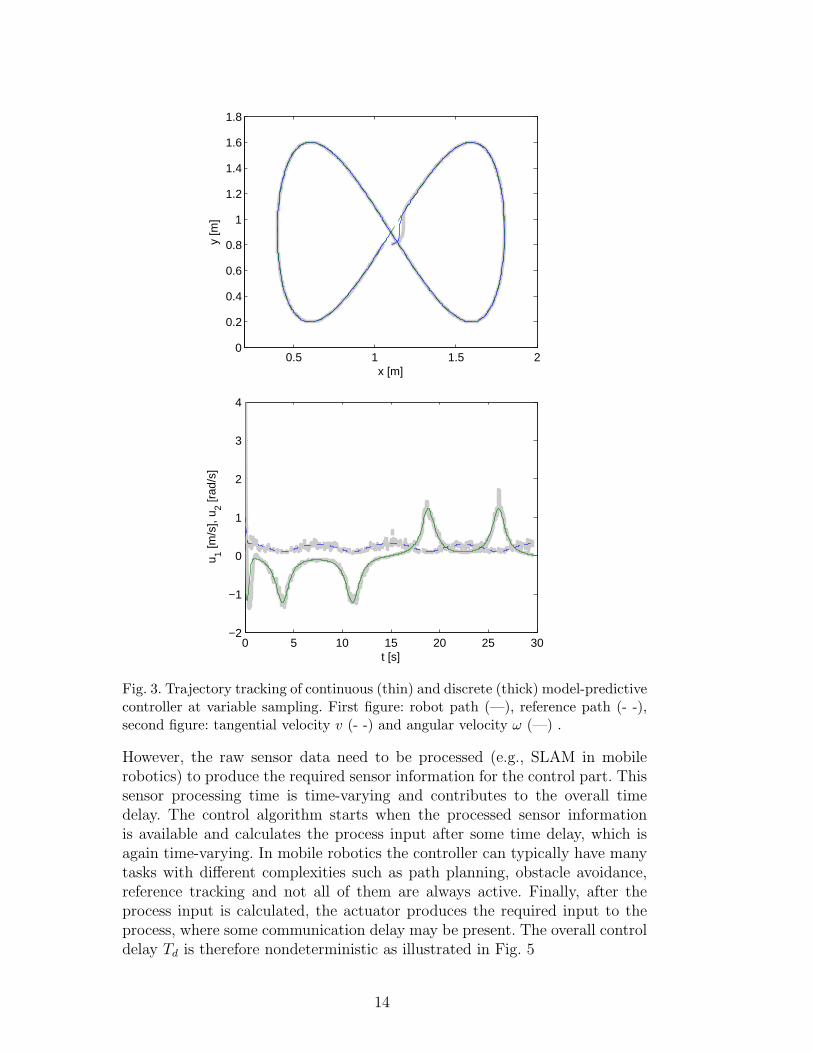
The results of the continuous MPC and discrete MPC are shown in Fig. 3.Due to the sample-time variation during the simulation (see Fig. 4), the noisein the control signals from the discrete MPC appears. This happens becausethe discrete control is not performed for regular periodic time samples and theerror due to the discretization is then propagated over the whole control-lawalgorithm.

12

0.5 1 1.5 20

0.2

0.4

0.6

0.8

1

1.2

1.4

1.6

1.8

x [m]

y [m

]

0 5 10 15 20 25 30−2

0

2

4

6

8

10

12

14

t [s]

v [m

/s],

ω [r

ad/s

]

Fig. 2. Trajectory tracking of continuous (thin) and discrete (thick) model-predictivecontroller at double sampling time (Ts = 0.066). First figure: robot path (—),reference path (- -), second figure: tangential velocity v (- -) and angular velocity ω(—) .

3.4 Performance under variable sampling and control delay

In practice, a control delay is present, which can again be modelled as anondeterministic process. The sensor processing, controller and actuators areusually event-driven parts of the closed-loop system. So, the sensor informationfor the control law starts processing as soon as the raw data from the physicalsensor is available, which can be assumed to be at regular sampling intervals Ts

or at nondeterministic intervals TsTrue (usually with quite a low uncertainty).

13

0.5 1 1.5 20

0.2

0.4

0.6

0.8

1

1.2

1.4

1.6

1.8

x [m]

y [m

]

0 5 10 15 20 25 30−2

−1

0

1

2

3

4

t [s]

u 1 [m/s

], u 2 [r

ad/s

]

Fig. 3. Trajectory tracking of continuous (thin) and discrete (thick) model-predictivecontroller at variable sampling. First figure: robot path (—), reference path (- -),second figure: tangential velocity v (- -) and angular velocity ω (—) .

However, the raw sensor data need to be processed (e.g., SLAM in mobilerobotics) to produce the required sensor information for the control part. Thissensor processing time is time-varying and contributes to the overall timedelay. The control algorithm starts when the processed sensor informationis available and calculates the process input after some time delay, which isagain time-varying. In mobile robotics the controller can typically have manytasks with different complexities such as path planning, obstacle avoidance,reference tracking and not all of them are always active. Finally, after theprocess input is calculated, the actuator produces the required input to theprocess, where some communication delay may be present. The overall controldelay Td is therefore nondeterministic as illustrated in Fig. 5

14

0 100 200 300 400 500 600 700 800 900 1000−0.01

0

0.01

0.02

0.03

0.04

0.05

0.06

0.07

0.08

sample

TsT

rue [s

]

Fig. 4. Sample-time variation during the simulation.

k(k-1) (k+1)

rawsensor

processedsensordata

calculatedcontrolaction

processactuator

TsTrue

Ta

Td

Fig. 5. Variable sampling demonstration. Raw sensor data are obtained at sampleintervals TsTrue, which triggers the processing algorithms to extract the requiredcontrol information from the raw sensor data. The latter triggers the control algo-rithms and finally the control variables are communicated to the process actuators.All the mentioned algorithms and the communication cause a control delay Td,which is usually nondeterministic as well as instants of the control inputs (actua-tion period Ta).

The results of the continuous and discrete MPC realization are shown in Fig.6. From the obtained results in Fig. 6 better performance is observed for thecontinuous MPC, where less noise appears in the control signal. The controldelay disturbs both control designs, which is seen from the noise in the controlsignals. However, due to the variable actuation period Ta the performance of

15

0.5 1 1.5 20

0.2

0.4

0.6

0.8

1

1.2

1.4

1.6

1.8

x [m]

y [m

]

0 5 10 15 20 25 30−2

−1

0

1

2

3

4

t [s]

u 1 [m/s

], u 2 [r

ad/s

]

Fig. 6. Trajectory tracking of continuous (thin) and discrete (thick) model-predictivecontroller at variable sampling and control delay. First figure: robot path (—),reference path (- -), second figure: tangential velocity v (- -) and angular velocity ω(—) .

the continuous controller realization is better as it has a faster response andlower noise at the control inputs. The variable period Ta is shown in Fig. 7and results from a nondeterministic sensor sampling and control delay.

In general, the noise at the control inputs is propagated from the processoutput noise and also from the noise in the sampling period and control delay.The faster the controller dynamics, the larger the control noise is. However,from Fig. 6 a faster response of continuous MPC is observed at a lower controlnoise than in discrete MPC.

16

0 100 200 300 400 500 600 700 8000

0.02

0.04

0.06

0.08

0.1

0.12

sample

Ta [s

]

Fig. 7. Sample time of actuation Ta varies due to the nondeterministic sensor sam-pling and the nondeterministic process delay.

Similar conclusions can also be made for the different reference trajectories.Example of a discontinues reference trajectory, which are usually the outputof path planing approaches [31], is given in Fig. 8.

3.5 Quality index comparison

A comparison of the performance for the simulated scenarios from Subsections3.1, 3.2, 3.3 and 3.4 is given in Table 1. The performance is evaluated by the

root-sum-square of the position error (RSSx =√∑

e2x, RSSy =

√∑e2

y) and

the orientation error (RSSθ =√∑

e2θ), by the norm of the root-sum-square of

the position errors (NSS =√

(RSS2x + RSS2

y)) from the reference trajectory

and by the standard deviations of the control inputs (σv, σω).

In first line of Table 1 an ideal situation is compared (Subsection 3.1) fromwhich it is clear that there is no noticeable difference in performance betweenthe continuous (CMPC) and the discrete (DMPC) realizations.

In the second line of Table 1 the robustness of the control design parameters tothe sampling period is tested (Subsection 3.2). The parameters optimized forthe sampling period Ts = 0.033 s are used on the simulation with the samplingperiod Ts = 0.066 s. It is clear that the performance (pose tracking and controlsignals) of the discrete realization performs much worse than the continuousone. It has to be noted that the RSS and NSS values of the second line andthe first line could not be compared due to the different number of sampling

17

0.5 1 1.5 20

0.2

0.4

0.6

0.8

1

1.2

1.4

1.6

1.8

x [m]

y [m

]

0 2 4 6 8 10 12 14−4

−2

0

2

4

6

t [s]

u 1 [m/s

], u 2 [r

ad/s

]

Fig. 8. Trajectory tracking with the continuous model-predictive controller at vari-able sampling and control delay. First figure: robot path (—), reference path (- -),second figure: tangential velocity v (- -) and angular velocity ω (—) .

instants for the same duration of the simulation.

In the third line of Table 1 a variable sampling is simulated (Section 3.3). Themain difference can be observed in the larger control-inputs noise standarddeviation of the DMPC, while the CMPC performs similarly to the in idealcase. In the DMPC the noise in the control signals is caused by the noise inthe sampling time, where the sampling instants are not periodic. Due to theclosed-loop operation the noise in the sampling time mostly affects the controlinputs, while the tracking errors are similar for the CMPC and DMPC.

In the fourth line of Table 1 a variable sampling and variable control delay

18

experiment method RSSx RSSy RSSθ NSS σv σω

[m] [m] [rad] [m] [m/s] [rad/s]

correct sampling CMPC 0.033 0.024 0.55 0.04 0.002 0.008

Ts = 0.033 DMPC 0.073 0.017 1.24 0.07 0.002 0.008

double sampling CMPC 0.021 0.025 0.24 0.035 0.003 0.016

Ts = 0.066 DMPC 0.068 0.030 1.07 0.075 0.005 0.018

variable sampling CMPC 0.110 0.210 93.6 0.23 0.002 0.009

TsTrue DMPC 0.123 0.214 94.9 0.25 0.059 0.064

variable TsTrue CMPC 0.112 0.233 85.9 0.26 0.024 0.052

and var. delay DMPC 0.130 0.269 93.2 0.30 0.086 0.099Table 1Performance of continuous and discrete control for the simulated scenarios evalu-ated by the root-sum-square of the pose errors and the standard deviations of thecontrols.

is simulated. The delay affects the performance of both control designs. Thevariable delay also contributes to a larger variance of the time between thesuccessive instants of the control-inputs update and, therefore increases thecontrol-inputs noise in the DMPC.

4 Experimental results

In the experiments the proposed continuous model-based predictive controlis compared to the discrete predictive control presented in [14]. Two mobilerobot platforms are used in experiments, a smaller two-wheeled mobile robotand four-wheeled Pioneer 3AT mobile robot (see Fig. 9). Both robot motioncan be approximated by differential kinematics but with different parameters.As already explained in section 2 (comment of Eq. (1)) the controller can alsobe applied to Ackermann robot type using simple velocities transformations.This covers majority of wheeled mobile robots used in practice.

The small robot is designed for robot soccer competitions where speed, robust-ness and accuracy are needed. It fits in a cube with a 7.5-cm side and weighs 0.5kg. The robot pose is estimated with an image sensor and a computer-visionalgorithm running at Ts = 0.033 s sampling. The maximum allowed tangentialvelocity and angular velocity were vMAX = 1m/s and ωMAX = 15rad/s, whilethe maximum allowed tangential wheel acceleration was aMAX = 3 m/s2. Pi-oneer 3AT is all-purpose outdoor mobile robot used mainly for research. Ituses laser range finder running with 10Hz (Ts = 0.1 s) for its localization.

19

Fig. 9. Small mobile robot (left) and Pioneer 3AT robot (right) used in experiments.

Maximum allowed velocities are set to vMAX = 0.8 m/s and ωMAX = 5 rad/s.

The optimal continuous feedback control law is derived in (29) and by takingthe first two rows of (HT TQH + TR)−1HT TQ(Fr −F ) the gain matrix Kc(t) isdefined for the applied control as follows

ub(t) = Kc(t)e(t), (32)

where e(t) is the undelayed system-tracking error, which is not available inpractice due to the different sources of system delay. The main delay sourceof the smaller robot is an image-based sensor delay where the current cameraimage needs to be precessed to obtain the robot pose. The other sources caus-ing an additional system delay are: the control algorithm computational timeand the communication delay. The overall delay is nondeterministic, whereTD = 2Ts is its estimated mean value. Delay of the Pioneer robot is less thanTs and is not compensated in the control.

The undelayed tracking error e(t) can be estimated from the delayed systemoutput ed(t) = e(t−Td) and the simulated system outputs em(t) and em(t−Td)using the Smith predictor scheme as follows

e(t) = ed(t) + em(t) − em(t − Td), (33)

which in the frequency domain reads

e(s) = ed(s) + (sI3 − A)−1Bu(s) − (sI3 − A)−1Be−sTdu(s), (34)

inserting (34) into the control law(32) defines the control input for the delayedsystem as follows

20

ub(s) = Kce(s) =

= Kced(s) + Kc(sI3 − A)−1B(I2 − e−sTd)ub(s)(35)

where Ij is the identity matrix of dimension j. The optimal controller transferfunction for the delayed system then reads

C(s) =ub(s)

yd(s)=

(I2 − Kc(sI3 − A)−1B(I2 − e−sTd)

)−1Kc, (36)

The same reference-trajectory and control-design parameters as selected insimulation section are used for the smaller robot. While the reference trajec-tory of the Pioneer robot is xr(t) = 1.4 sin

(2πt50

), yr(t) = 1.4 sin

(4πt50

)and

design parameters for CMPC are: Th = 4Ts

Q =

⎡⎢⎢⎢⎢⎢⎣

1 0 0

0 5 0

0 0 0.2

⎤⎥⎥⎥⎥⎥⎦ , R =

⎡⎢⎣ 0.3 0

0 0.3

⎤⎥⎦ , Ar =

⎡⎢⎢⎢⎢⎢⎣−3 0 0

0 −3 0

0 0 −3

⎤⎥⎥⎥⎥⎥⎦

The control parameters for both control laws (CMPC and DMPC) are selectedequivalently to have the same performance.

The trajectory-tracking results (for the small robot), obtained using the pro-posed continuous model-predictive controller (CMPC) and comparison to dis-crete model-predictive controller (DMPC), are shown in Fig. 10 The trajectory-tracking results of both approaches are of approximately similar quality. Bothresult in good tracking in the presence of the system delay and noisy sensordata, with a standard deviation of approximately 2 mm for position and 1◦ fororientation. During the experiments sensor disturbances, such as the wrongpose estimation (outliers; 2% of all measurements) and some camera distortion(perspective and radial distortion) are also present.

A closer comparison of trajectories in Fig. 10 reveals slightly better track-ing results for the CMPC during the initial transition. This is also seen inthe comparison of the quality indexes in the first row of table Table 2. Themain difference between both approaches is observed by comparing velocityinputs.A much higher jitter in the tangential and angular velocity is presentin the discrete model predictive control, which is also seen from the standarddeviations of the control variables in the first row of table Table 2.The lat-ter statement was observed in experiment as a much smoother motion of therobot platform in the case of the CMPC.

More detailed validation is done for the Pioneer robot using constant sampling,double sampling and variable sampling as follows in Figs. 11- 13 and in table

21

0.4 0.6 0.8 1 1.2 1.4 1.6 1.80.2

0.4

0.6

0.8

1

1.2

1.4

1.6

x [m]

y [m

]

0 5 10 15 20 25 30−2

−1

0

1

2

3

4

5

6

t [s]

v [m

/s],

ω [r

ad/s

]

Fig. 10. Trajectory tracking experiment of the small robot with the CMPC (thin)and DMPC (thick). at variable sampling and control delay. First figure: robot path(—), reference path (- -), second figure: tangential velocity v (- -) and angularvelocity ω (—).

2. From figures and table of performances the same conclusions can be drawnas in section 3. Continuous and discrete approaches are equivalent at regularsampling time where actual sampling time is the same as the one selectedin the tuning phase (see Fig. 11). If sampling time is changed (in Fig. 12is doubled so Ts = 0.2 s) and the control design parameters are not adapted(they are valid for Ts = 0.1 s) then the performance od DMPC becomes worsewhile the CMPC performance is not affected noticeably. Similarly if samplingtime is changing randomly then the performance of DMPC becomes worsewhile the CMPC is insensitive to the sampling time period variation (in Fig.13 sample is lost with 50% probability).

22

−1.5 −1 −0.5 0 0.5 1 1.5

−1

−0.5

0

0.5

1

x [m]

y [m

]

0 10 20 30 40 50 60−1.5

−1

−0.5

0

0.5

1

1.5

t [s]

u 1 [m/s

], u 2 [r

ad/s

]

Fig. 11. Trajectory tracking experiment of Pioneer robot with the CMPC (thin) andDMPC (thick) at regular sampling time Ts = 0.1 s. First figure: robot path (—),reference path (- -), second figure: tangential velocity v (- -) and angular velocity ω(—).

From the above comparisons the CMPC approach gives better results, whichis to be expected because of the varying sampling times, mostly due to thevariable control delay. The CMPC algorithm is derived in continuous spaceand therefore the discretization of the continuous system tracking model (7) isnot needed, as it is in the case for the DMPC. This statement is also consistentwith the simulation analysis made.

In the DMPC the tracking-error model discretization according to the desiredsample time is made. Because the actual sampling time instants are nondeter-ministic, the error due to the discretization is then propagated over the whole

23

−2 −1.5 −1 −0.5 0 0.5 1 1.5

−1.5

−1

−0.5

0

0.5

1

x [m]

y [m

]

0 10 20 30 40 50 60−5

0

5

t [s]

u 1 [m/s

], u 2 [r

ad/s

]

Fig. 12. Trajectory tracking experiment of Pioneer robot with the CMPC (thin) andDMPC (thick) at double sampling time (Ts = 0.2 s) and control design parameterstuned to Ts = 0.1 s. First figure: robot path (—), reference path (- -), second figure:tangential velocity v (- -) and angular velocity ω (—).

control-law algorithm, while in the CMPC the continuous control signal isonly evaluated in actual discrete time samples at the end of each control-loopiteration before sending the velocity commands to the robot platform.

5 Conclusion

The continuous model-predictive trajectory-tracking control of a mobile robotis presented in this paper. The proposed control law minimizes the quadratic

24

−2 −1 0 1 2

−1.5

−1

−0.5

0

0.5

1

1.5

x [m]

y [m

]

0 10 20 30 40 50−3

−2

−1

0

1

2

3

t [s]

u 1 [m/s

], u 2 [r

ad/s

]

Fig. 13. Trajectory tracking experiment of Pioneer robot with the CMPC (thin) andDMPC (thick) at variable sampling time where sample is lost with 50% probability.First figure: robot path (—), reference path (- -), second figure: tangential velocityv (- -) and angular velocity ω (—).

cost function consisting of tracking errors and control effort as is also thecase in the discrete version. The solution to the control is derived analyti-cally, which enables fast, real-time implementations. The proposed continuousmodel-predictive control was validated by simulation and also on a real mobilerobot.

Continuous model-predictive control design has, in ideal situations, similarperformance to the equivalent discrete model-predictive control. However, ingeneral situations the assumption of having a uniform sampling time and adeterministic control delay is not always realistic. It has been shown that a con-

25

experiment method RSSx RSSy RSSθ NSS σv σω

[m] [m] [rad] [m] [m/s] [rad/s]

small robot

sampling CMPC 0.31 0.83 3.27 0.88 0.032 0.53

Ts = 0.033 DMPC 0.32 0.90 3.88 0.95 0.055 0.78

Pioneer robot

CMPC 0.66 1.24 1.14 1.41 0.039 0.038

Ts = 0.1 DMPC 0.99 1.50 1.11 0.95 0.051 0.105

Pioneer robot

CMPC 0.53 0.97 1.04 1.11 0.027 0.036

Ts = 0.2 DMPC 8.35 5.88 4.46 10.21 0.315 1.383

Pioneer robot

CMPC 0.61 1.1 1.01 1.26 0.041 0.042

variable Ts DMPC 3.10 4.67 3.48 5.61 0.258 0.812Table 2Performance of CMPC and DMPC for experiments on real robots evaluated by theroot-sum-square of the pose errors and the standard deviations of the controls.

tinuous design gives better results in cases where the sampling-time instantsare not deterministically periodic. An important advantage of the proposedcontinuous model predictive control is also the better robustness of its control-law design parameters according to the sampling period. The change in thesampling period does not affect the control quality.

References

[1] A. Balluchi, A. Bicchi, A. Balestrino and G. Casalino, Path Tracking Controlfor Dubin’s Cars, in: Proceedings of the 1996 IEEE International Conferenceon Robotics and Automation, Minneapolis, Minnesota, 1996, pp. 3123-3128.

[2] R. W. Brockett, Asymptotic stability and feedback stabilization, in: R. W.Brockett, R. S. Millman, and H. J. Sussmann, eds., Differential GeometricControl Theory, Birkhuser, Boston, MA, 1983, pp. 181-191.

[3] S. Blazic, A novel trajectory-tracking control law for wheeled mobile robots,Robotics and Autonomous Systems, 59(11) (2011) 1001-1007.

[4] C. Canudas de Wit and O. J. Sordalen, Exponential Stabilization of MobileRobots with Nonholonomic Constraints, IEEE Transactions on AutomaticControl, 37(11) (1992) 1791-1797.

26

[5] D. Gu and H. Hu, Neural predictive control for a car-like mobile robot, Roboticsand Autonomous Systems, 39(2) (2002) 73-86.

[6] Y. Kanayama, Y. Kimura, F. Miyazaki and T. Noguchi, A stable trackingcontrol method for an autonomous mobile robot, in: Proceedings of the 1990IEEE International Conference on Robotics and Automation, Vol. 1, Cincinnati,OH, 1990, pp. 384-389.

[7] D.-H. Kim, J.-H. Oh, Tracking control of a two-wheeled mobile robot usinginput-output linearization, Control Engineering Practice, 7(3) (1999) 369-373.

[8] I. Kolmanovsky and N. H. McClamroch, Developments in NonholonomicControl Problems, IEEE Control Systems, 15(6) (1995) 20-36.

[9] F. Kuhne, W. F. Lages and J. M. Gomes da Silva Jr., Model Predictive Controlof a Mobile Robot Using Linearization, in: Proceedings of Mechatronics andRobotics 2004, Aachen, Germany, 2004.

[10] T. C. Lee, K. T. Song, C. H. Lee and C. C. Teng, Tracking control ofunicycle-modeled mobile robots using a saturation feedback controller, IEEETransactions on Control Systems Technology, 9(2) (2001) 305-318.

[11] A. Luca and G. Oriolo, Modelling and control of nonholonomic mechanicalsystems, in: J. Angeles and A. Kecskemethy, eds., Kinematics and Dynamics ofMulti-Body Systems, Springer-Verlag, Wien, 1995.

[12] A. Luca, G. Oriolo and C. Samson, Feedback control of a nonholonomic car-like robot, in: J. P. Laumond ed., Robot Motion Planning and Control, LecturesNotes in Control and Information Sciences, Vol. 229, Springer-Verlag, London,1998, pp. 171-253.

[13] A. Luca, G. Oriolo and M. Vendittelli, Control of wheeled mobile robots: Anexperimental overview, in: S. Nicosia, B. Siciliano, A. Bicchi and P. Valigi, eds.,RAMSETE - Articulated and Mobile Robotics for Services and Technologies,Springer-Verlag, 2001.

[14] G. Klancar, I. Skrjanc, Tracking-error model-based predictive control for mobilerobots in real time. Robot. auton. syst., vol. 55, iss. 6, pp. 460-469, 2007.

[15] S. P. M. Noijen, P. F. Lambrechts and H. Nijmeijer, An observer-controllercombination for a unicycle mobile robot, International Journal of Control, 78(2)(2005) 81-87.

[16] J.E. Normey-Rico, J. Gomez-Ortega and E.F. Camacho, A Smith-predictor-based generalised predictive controller for mobile robot path-tracking, ControlEngineering Practice, 7(6) (1999) 729-740.

[17] A. Ollero and O. Amidi, Predictive Path Tracking of Mobile robots. Applicationto the CMU Navlab, in: Proceedings of 5th International Conference onAdvanced Robotics, Robots in Unstructured Environments (ICAR ’91), Vol.2, Pisa, Italy, 1991, pp. 10811086.

27

[18] G. Oriolo, A. Luca and M. Vandittelli, WMR Control Via Dynamic FeedbackLinearization: Design, Implementation, and Experimental Validation, IEEETransactions on Control Systems Technology, 10(6) (2002) 835-852.

[19] K. Park, H. Chung, and J. G. Lee, Point stabilization of mobile robots viastate-space exact feedback linearization, Robotics and Computer IntegratedManufacturing, 16 (2000) 353-363.

[20] F. Pourboghrat and M. P. Karlsson, Adaptive control of dynamic mobilerobots with nonholonomic constraints, Computers and electrical Engineering,28 (2002) 241-253.

[21] F. M. Raimondi and M. Melluso, A new fuzzy dynamics controller forautonomous vehicles with nonholonomic constraints, Robotics and AutonomousSystems, 52 (2005) 115-131.

[22] C. Samson and K. Ait-abderrahim, Feedback control of a nonholonomic wheeledcart in Cartesian space, in: Proceedings of the 1991 IEEE InternationalConference on Robotics and Automation, Vol. 2, Sacramento, CA, 1991, pp.1136-1141.

[23] C. Samson, Time-varying feedback stabilization of car like wheeled mobilerobot, International Journal of Robotics Research, 12(1) (1993) 55-64.

[24] N. Sarkar, X. Yun and V. Kumar, Control of mechanical systems with rollingconstraints: Application to dynamic control of mobile robot, The InternationalJournal of Robotic Research, 13(1) (1994) 55-69.

[25] K.J. Astrom and B. Wittenmark, Computer-Controlled Systems, Theory andDesign. Prentice Hall, 1996.

[26] J. Nilsson, Real-Time Control Systems with Delays. Department of AutomaticControl Lund Institute of Technology, Lund, 1998.

[27] H.A. van Essen and H. Nijmeijer, Nonlinear model predictive control forconstrained mobile robots, in: European control conference: ECC ’01, Porto,Portugal, 2001, pp. 1157-1162.

[28] S. Adinandra, E. Schreurs and H. Nijmeijer, A Practical Model PredictiveControl for a Group of Unicycle Mobile Robots, in: 4th IFAC Nonlinear ModelPredictive Control Conference, Vol. 4, No. 1, Leeuwenhorst, Netherlands, 2012,pp. 472-477.

[29] G. Dudek, M. Jenkin, Computational Principles of Mobile robotics, Secondedition. Cambridge University Press, 2010.

[30] E. Kayacan, H. Ramon, W. Saeys, Robust Trajectory Tracking Error Model-Based Predictive Control for Unmanned Ground Vehicles, IEEE/ASMETransactions on Mechatronics, 21(2) (2016) 806-814.

[31] C. Purcaru, R.-E. Precup, D.T. Iercan, R.C. David, Hybrid PSO-GSA robotpath planning algorithm in static environments with danger zones, in: 17thInternational Conference: System Theory, Control and Computing (ICSTCC),2013, pp. 434-439.

28

[32] M. Wargui, M. Tadjine, A. Rachid, Stability of real time control of anautonomous mobile robot, in: 5th IEEE International Workshop on Robot andHuman Communication, 1996, pp. 311-316.

[33] M.F. Sagfors, H.T. Toivonen, H infinity and LQG control of asynchronoussampled-data systems, Automatica, 33(9) (1997) 1663-1668.

[34] H. Gao, T. Chen, Stabilization of Nonlinear Systems Under Variable Sampling:A Fuzzy Control Approach, IEEE Transactions on Fuzzy Systems, 15(5) (2007)972-983.

29