A Comparative Study of Operational Vessel Detectors for

1

A Comparative Study of Operational VesselDetectors for Maritime Surveillance usingSatellite-borne Synthetic Aperture RadarMattia Stasolla, Jordi J. Mallorqui, Gerard Margarit, Carlos Santamaria, Nick Walker

Abstract—This paper presents a comparative study comparingfour operational detectors that work by automatically post-processing Synthetic Aperture Radar (SAR) images acquiredfrom the satellite platforms RADARSAT-2 and COSMO-SkyMed.Challenging maritime scenarios have been chosen to assess thedetectors’ performance against features such as ambiguities,significant sea clutter or irregular shorelines. The SAR imageswhich form the test data are complemented with ground-truthto define the reference detection configuration, which permitsquantifying the Probability of Detection (PoD), the False AlarmRate (FAR) and the accuracy of estimating ship dimensions.Although the results show that all the detectors perform notablywell, there is no perfect detector, and in future work a betterdetector could be developed that combines the best elements fromeach of the detectors. Beyond the pure comparison exercise,the study has permitted improving the detectors by pointingweaknesses out and providing means for fixing them.

Index Terms—Ship detection, maritime surveillance, maritimesecurity, satellite imaging, SAR.

I. INTRODUCTION

SHIP detection by post-processing satellite SynthethicAperture Radar (SAR) images is a remote sensing based

application that has been a subject of a lot of studies [1], [2],[3], [4]. Having practical interests in the security maritimedomain, ship detection using SAR data has gained popularitythanks to the sensors’ large swath widths and their ability tofunction during all weathers and during the night time as wellas when there is daylight. In addition, in many circumstancesthe backscattered signal from a ship is much larger than thesea background so at the most basic level detection is achievedby searching for pixels with amplitudes greater than a given

Manuscript received September 30, 2015; revised Month Day, 2016.The research leading to these results has received funding from the Eu-

ropean Union Seventh Framework Programme (FP7/2007-2013) under grantagreement n◦ 263468 (NEREIDS).

RADARSAT-2 Data and Products c©MacDonald, Dettwiler and AssociatesLtd. 2013 - All Rights Reserved – RADARSAT is an official mark of theCanadian Space Agency, provided under COPERNICUS by the EuropeanUnion. COSMO-SkyMed images c©ASI 2013, distributed by e-GEOS S.p.A.,provided under COPERNICUS by the European Union and ESA, all rightsreserved.

M. Stasolla and C. Santamaria are with the Institute for the Protectionand Security of the Citizen, Joint Research Centre, European Commission,I-21027 Ispra, Italy.

J. J. Mallorqui is with the Remote Sensing Lab (RSLab), Department ofSignal Theory and Communications, Universitat Politecnica de Catalunya(UPC), 08034 Barcelona, Spain.

G. Margarit is with the Remote Sensing Application and Services (RSAS)Division, GMV Aerospace and Defence, S.A.U.

N. Walker is with eOsphere Limited, Satellite Applications Catapult (R103),Harwell Space Cluster, Fermi Avenue, OX11 0QR, UK.

scattering threshold [5]. However, in reality there are severalphenomena that add confusion to the overall process and biasthe perfect model into something unpredictable [6], [7].

In recent years vessel detection performance has beenimproved by evolutions in technology, for example by in-creasing the number of information channels (through po-larimetry), improving the resolutions (sub-metric resolutionsare possible) and increased coverage. In addition, new platformand constellation configurations have been put in place toprovide response to the more challenging demands that usersare requesting, such as reduced latency times (between dataacquisition and detection output) or detection capability forsmaller ships of interest [8], [9].

Despite this technological evolution, ship detection is notcurrently yet free from complex artefacts that reduce perfor-mance for a range of scenarios, which are of interest formany users. The new techniques that have been proposedover recent years to exploit all the technological potentialitieshave provided a quality step forward in terms of robustnessand probability of detection (PoD). However, they are not yetrobust enough against ambiguities, strong scatterers, irregularshorelines or sea clutter [10], [11], [12].

The current paper addresses these problems, which mostadversely affect ship detection performance, and presents acomparative study among four operational ship detectors. Thegoal was to quantify the performance of each of them fora set of challenging configurations and propose improvementactions to overcome the drawbacks or at least to reduce theirinfluence in the final results.

The work presented in this paper has been carried outin the framework of the FP7 NEREIDS project, an Euro-pean Commission co-financed project with the main goalto improve ship monitoring techniques [13]. Four detectorshave been analysed: 1) SUMO from Joint Research Centreof the European Commission (JRC) [14]; 2) UPC-WT fromUniversitat Politecnica de Catalunya (UPC) [15]; 3) SIDECARfrom GMV Aerospace and Defence (GMV) [16]; and 4) R&Gfrom eOsphere Limited (eOsphere) [17].

These are of course only some of the providers that cancurrently offer operational ship detection by satellite SAR(which, to the best of our knowledge, are no more thanfifteen). Nevertheless, the detection systems here analyzed canbe considered a proper representative sample1 so that their per-

1Given that each detector has its own specific features, in many cases, thebackground theories overlap.

2

formance assessment would provide very useful informationabout the actual technological capacity in this field.Moreover, the latest detailed performance assessment of shipdetection system reported in literature dates back to 2007 [18],when a comparative exercise among nine different detectorswas run within the DECLIMS project to know what qualityshould have been expected at that time from satellite shipdetection services, and to understand how to improve theirproducts. The present work would therefore be helpful toupdate those results and provide new insights.

This paper is organized as follows. Section II provides abrief description of the four detection systems under analysis.In Section III the methodology employed for the comparativestudy is discussed, focusing on the scope of the exerciseand the evaluation procedure. Section IV is devoted to thedescription of the dataset employed for the analysis and thereview of the results. Final comments and future remarks aregiven in Section V.

II. BACKGROUND

Table I summarizes the main characteristics, at the timeof the study, of the four operational detectors under review,whose brief description is provided hereafter. As can be seen,the softwares are based on different detection algorithms andthey can support a number of sensor/image products. They arealso supplied with advanced processing features, such as landmasking and the removal of azimuth ambiguities.

1) SUMO: The JRC has developed in the past yearsan algorithm for vessel detection called SUMO (Searchingfor Unidentified Maritime Objects), shown in operation inFigure 1. The SUMO ship detector adopts a fast version ofa K-distribution CFAR detector [14]. SUMO has been imple-mented in Java and is available for all computer platformssupporting the Java Virtual Machine [19]. The main advantageof the algorithm is the performance in terms of detection speedand robustness.

The K-distribution model depends on 3 parameters [20]: themean, the number of looks, an instrument factor essentiallydescribing the noise that is introduced by the radar image, andthe shape factor, which determines the width of the distributionand it reflects the actual variation of radar backscatter valueson the sea surface. In SUMO the size of the sub-image tile toestimate these parameters is of the order of 200× 200 pixels.

Once the parameters of the probabilistic distribution havebeen estimated, and a value for the probability of false alarm(PFA) is chosen, the false alarm threshold t can be determined.Since the estimation of the unknown parameters might bebiased by the presence of high-valued target pixels in the tile,these ones are excluded from the calculation. This operation isnamed clipping. In practice, the 1% highest pixels in the tileare discarded from the mean and order parameter computation.However, strictly applying the threshold calculated after theclipping process gives many false alarms. Presumably this isbecause the K-distribution does not perfectly represent the seaclutter in all situations, e.g. when the presence of ocean wavesor atmospheric phenomena bias the tile statistics. Thereforea second, higher, threshold is defined based on a significance

Code:

Date:

Version:

Page:

NEREIDS GMV 2015; all rights reserved Error! Unknown document property name.

NEREIDS_D310

21-12-2011

1.0

102 of 142

Figure 3-20 Snapshots from SUMO in operation. Labels: [A] is the main SUMO application window and in blue squares are shown the detected vessels, [B] is the K-distribution threshold and buffer zone dialog entry parameters, [C] is the histogram versus threshold window which shows the impact of

threshold selection on the detected targets, [D] is the process layers, namely the Image Name, the GSHHS land mask for this image and the vessel detection (VDS) analysis results which is shown in

more detail in [E].

3.3.6.2. Satlantic

The Ocean Monitoring Workstation (OMW) is Satlantic's tool of maritime surveillance using SAR images. It handles ERS, RADARSAT-1, and RADARSAT-2 images, and it is able to apply vessel detection, oil spill detection, wind information retrieval, wave spectrum analysis and sea state analysis.

The vessel detection module is based on CFAR k distribution generally and adopts a χ2 distribution for

Radarsat-2. In addition to the location of the target, it also obtains its length and beam using calculations based on principal components analysis. Detection are displayed on the original imagery and on maps.

The oil spill detection algorithm searches for dark areas as potential instances of oil contamination.

Fig. 1. SUMO: snapshot in operation. Labels: (A) is the main SUMOapplication window and in blue squares are shown the detected vessels, (B)is the K-distribution threshold and buffer zone dialog entry parameters, (C) isthe histogram versus threshold window which shows the impact of thresholdselection on the detected targets, (D) is the process layers, namely the ImageName, the GSHHG land mask for this image and the vessel detection analysisresults which is shown in more detail in (E).

parameter that measures the difference between the pixel valuex and the mean of the tile.

In order to avoid detection of inland targets, land maskingis applied and SUMO uses the publicly available Global Self-consistent Hierarchical High-resolution Shoreline (GSHHG)database [21]. The land mask is not always accurate, depend-ing on several factors, such as the original source and scaleof the shoreline information, tidal differences, etc. Hence, abuffer zone having a constant distance from the land (shore)is applied and the detection takes place outside the maskedand buffered zones.

Following the detection, pixel clustering is applied and de-tected pixels are agglomerated into targets (vessels). For eachvessel then the number of pixels, position, length, width andheading are estimated. Finally, detections likely to be azimuthambiguities are removed by using the SAR parameters. Thisstep makes use of the deterministic distance that separates anambiguity from the scatterer that originates that ambiguity. Ifa detection is located at that ambiguity distance from a muchstronger scatterer, that detection is classified as an ambiguityand removed.

At the moment of the exercise, SUMO supported thefollowing SAR imagery formats: Envisat Images and ERS2,RADARSAT-1 (CEOS format), RADARSAT-2, TerraSAR-X,COSMO-SkyMed (later on Sentinel-1 has been added).The detection output has the form of Comma Separated Values(csv), shapefile, xml, gml (KSAT schema), kmz (GoogleEarth), postgis or thumbnails.

2) UPC-WT: UPC has developed during the last yearsan algorithm for vessel and coast detection that uses theWavelet Transform (WT) through a multi-scale analysis basednot only on the intensity on SAR images but consideringalso its localized statistical behaviour. At fine scales, theWT provide information about the variation of a functionaround a point. Thus, irregularities (edges) are sharpened in theparticular direction of each sub-band (i.e. vertical, horizontaland diagonal). The WT does not remove from the sub-bandsthe most local dependencies due to regular spatial structuresand patterns. The different scales and bands are combineddifferently depending on the application.

3

Name Organization Sensors supported Land masking Ship detectiontheory Additional features

SUMOJoint Research Centre,European Commission(JRC)

Envisat, ERS2,RADARSAT-1,RADARSAT-2,COSMO-SkyMed,TerraSAR-X

Shapefile withbuffer zone

CFAR withK-distributionbackground

Azimuth ambiguities;Ships that are too long ortoo wide are rejected

SIDECARGMV Aerospace andDefense, S.A.U.(GMV)

Envisat, ERS2,RADARSAT-1,RADARSAT-2, COSMO-SkyMed, TerraSAR-X,ALOS-PALSAR

Shapefile withbuffer zone;Shapefilesautomaticallyextracted fromimage

Cluster-basedapproach based onWavelet Transform

Azimuth ambiguities;Geodetic Active Contoursto delineate target contour;Inclusion of targetcategorization withassociated confidence

UPC-WT

Remote Sensing Lab(RSLab),Universitat Politecnicade Catalunya (UPC)

Envisat, ERS2,RADARSAT-1,RADARSAT-2,COSMO-SkyMed,TerraSAR-X,ALOS-PALSAR

Shapefile withbuffer zone;Shapefilesautomaticallyextracted fromimage

CFAR withgaussian-distributionbackground based onWavelet Transform

Azimuth ambiguities;Ships that are above orbelow a given size arerejected.

R&G eOsphere Limited

Envisat, ERS2,RADARSAT-1,RADARSAT-2,COSMO-SkyMed,TerraSAR-X, ALOS-PALSAR

Shapefile withbuffer zone

Median filters, toseparate targets frombackground;Pauli decompositionchannels for quad-pol

No Azimuth ambiguities;Histogram of the detectedpixel for outliers andfitting an ellipse to theremaining detected pixels.

TABLE ISHIP DETECTION SYSTEMS.

Vessel detection: The ship is usually noticeable in the threesub-bands after the 2-D WT, but the values of the pixels ofthe background clutter are in general randomly distributed.For vessel detection, the algorithm works by exploiting thesecharacteristics by spatially multiplying the four components(low-pass filter version of the original image plus three sub-bands) resulting from each iteration and proceeding to thedetection directly in the wavelet domain. This is known asintra-scalar processing of the WT. With this technique there isan enlargement of the dynamic range due to the multiplicationprocess involved. The histogram of the resulting image isadjusted to a Gaussian, it has been seen that this distributionadjusts very well to the sea clutter after the WT process quiteindependently of the original clutter distribution. Dependingon the selected Probability of False Alarm (PFA) the properthreshold is selected, as in a classical CFAR approach. Acomplete description of the algorithm can be found in [15],[22].

If the coast is not perfectly masked, it has an important influ-ence when calculating the detection thresholds under a CFARapproach. The presence of the coast modifies the histogramand thus the threshold. The adjustment of the histogram to adouble Gaussian helps to reduce the chances or an incorrectestimation of the threshold.

All detections are post-processed with morphological fil-ters [23] to eliminate targets which size makes them to benon-realistic vessels (for instance a large non-masked islandor too small targets) and an ambiguity detector to eliminatethose detections associated to ambiguities, either from vesselsor coastal features. The implemented algorithm also includesmodules to make some improvements in the image to facilitate

the classification of the detected vessels. For instance, theSingular Value Apodization (SVA) is a non-linear filter ableto eliminate the sidelobes of strong scatters visible in lowreflectivity areas [24]. The software also includes tools forvessel size and orientation.

Land masking: The inaccuracies of GSHHG shoreline pub-lic databases can produce many false alarms when workingwith images containing coast. Usually, the way to deal withsuch inaccuracies is to expand the coastline towards the sea,for instance 100 m. This solution can be effective with simplecoastlines but it fails with convoluted ones. One option is toextract the coastline from the image itself. UPC-WT uses theproperties of the inter-scalar processing of Wavelet Transform(WT) to enhance the edges to carry out a coastline extrac-tion [25]. Figure 2 shows the final result with the extractedcoastline. As it can be seen it perfectly matches the SAR imageand it is more precise than the GSHHG one.

The detection report for UPC-WT can be provided in twooutput formats: csv and kmz.

3) SIDECAR: GMV has developed a Ship MonitoringService (SIMONS) that provides maritime surveillance byautomatically post-processing any type of Earth Observation(EO) image and AIS2 streams [16]. The EO-based ship detec-tion and categorization stage is covered by the Ship Detectionand Categorization Runtime (SIDECAR) that can post-processeither any type of SAR (any imaging mode, sensor and format)or optic image. SIDECAR has been designed to be modular,flexible, reliable and unsupervised (no human operator sup-port). Four main high-level stages can be differentiated:

2Automatic Identification System (AIS) is an automatic tracking systemintroduced for identifying and locating vessels [26].

4

Fig. 2. UPC-WT: WT Coastline extraction (green) compared with GSHHGcoastline (yellow).

Data acquisition: this stage consolidates input data intosystem repository.

Information extraction. This stage isolates and estimates allthe information that is needed from EO images. There arethree main sub-modules:

- Coastline Delineation (CD): the module isolates thecoastline present in a SAR image by using externalshape files and/or an algorithm that combines WaveletTransform (WT) [27] and Geodesic Active Contours(GAC) [28], [29]. WT enhances the scattering informationof land, while GAC delineates the contour via an energy-based minimization function.

- Ship Detection (SD): The module detects the shipspresent in a EO image and derives the so-called VesselDetection System (VDS) reports, shown in Figure 3.SAR images are post-processed via a multi-scale clus-tering method based on WT. Differently from UPC-WT(which makes use of WT only), here the detector firstcombines the intermediate WT products by applying apoint-wise multiplication among them and then identifiesclusters of pixels that allow to detect targets regardlessof their proximity and morphology. This also permitsto estimate a confidence parameter that quantifies howreliable a detected target is. Finally, azimuth ambiguitiesare removed.

- Ship Categorization (SC): The module analyses the dis-tribution of the reflectivity values along the SAR shipsignature to make ship categorization via Fuzzy Logic(FL) [30]. Whenever possible, a wake detector is used todetermine ship speed and course, increasing the discrim-ination sensitivity.

Added-value: This stage provides added-value features:- AIS processing that correlates ship detection reports with

AIS polls. Fuzzy logic is used to quantify the correlationpercentage and refine the SAR-based VDS position bycompensating the slant-range projection and the azimuthshifts caused by target dynamics.

- Anomaly detection by processing cooperative data andthe VDS reports.

Result Dissemination. This stage delivers final products tousers via a large set of output formats and channels. Plaintext files or complex xml files that are compliant with theEMSA standards can be selected. Automatic integration with

Code:

Date:

Version:

Page:

NEREIDS © GMV 2012; all rights reserved D310.1 State of the Art

NEREIDS_D310

21-12-2011

1.0

116 of 142

o ship classification: heading and dimension of the detected targets are computed. The algorithm also finds the normalised RCS of the bow, middle and stern sections, and

applies fuzzy logic processing to classify the detection in a number of vessel categories (tanker, container ship…).

- AIS processing: VDS detections are correlated with AIS messages. This is done by using the

AIS tracks to estimate the position of the target in the SAR images. For each target correlated, a confidence measure is computed using the distance between the predicted and actual location of the target and the similarity between SAR-estimated and AIS-reported ship

heading and dimension.

The final products can be delivered to the users via a web interface or via email, FTP or other methods in text, XML, Google Earth… format. For each ship the reports contain the following information:

location, detection confidence, ship category, classification confidence, heading, length, breadth and normalised RCS of the bow, middle and stern sections.

Figure 3-33 GMV SIMONS: snapshots of the ship detection

3.3.6.9. DLR

DLR’s ship detection tool is CFAR-based and assumes a Gaussian distribution of the background clutter. The pixel under test is surrounded by three areas of increasing size (target, guard and

background). The sizes of these areas are determined by the image resolution and the size range of the ships expected. The background area is used to estimate the parameters of the probability density function (Gaussian) of the sea background. The desired false alarm rate is chosen as a design parameter. The threshold that satisfies the false alarm rate for the estimated background parametric

distribution is computed. If the pixel under study has a value greater than the threshold, it will be classified as a detection.

GSHHS is used for land masking, with a buffer zone width selected by the user. This is to prevent the detection algorithm from being applied to land areas, which would produce a large number of invalid detections.

AIS messages are included automatically to determine cooperative vessels detected in the SAR images.

After the CFAR-based ship detection stage, an algorithm to reject azimuth ambiguities is applied. The distance from azimuth ambiguities to point targets is calculated based on the system design. Azimuth ambiguities of detected ships are excluded. As for strong land scatterers, a couple of SAR images are

used to create lookup tables of scatterers and ambiguities. These tables are then applied to the images under investigation to reject ambiguities of land scatterers.

Fig. 3. SIDECAR: snapshot of the ship detection report and coastlineisolation (blue line). Confidence is colour-coded from red (0 – minimum)to green (1 – maximum).

SIMONS is possible through dedicated databases.

4) R&G: The R&G ship detection algorithm developedat eOsphere Limited was originally designed to exploit fullypolarimetric data, such as that available from the RADARSAT-2 satellite. However, the algorithm was also adapted for usewith dual and single polarisation data [17] that was availableas a part of the NEREIDS project. For the single polarisationcase, i.e. for the results presented in this paper, the algorithmreduced to the use of a median filter followed by a series ofmorphological operations.

In order to find an estimate of the background signal fromthe ocean, each pixel under consideration is surrounded bya guard area to ensure that no pixel of an extended targetcould be considered as a part of the background. The widthof the guard region is set by the user to a suitable valuebased on the expected size of possible vessels. In order tocounteract the influence of outlying values, the median valueof the background values is calculated and compared againstthe pixel under consideration. The calculation of the medianis generally slower than for the mean, however, the resultingalgorithm provides more reliable results.

Pixels are designated as “detected” when they are more thanX times that of the median of the values from the background.During the course of the experiment a range of different valuesof X were tested and a value of X = 3 was found to give agood level of target detection versus unwanted false alarms.

The resulting binary detection image is then filtered usingmorphological operations [31] to remove features in the detec-tion image that would be unlikely to occur in reality.The first morphological operation is the fill function, whichfills isolated interior pixels, i.e. individual 0s surrounded by1s. The second morphological operation is the bridge function,which sets 0-valued pixels to 1 if they have two non-zeroneighbours that are not connected. Moreover, in order toprevent the detection algorithm from being applied to landareas, a masking procedure is employed utilising the freelyavailable GSHHG shoreline.

The output from the “classification” module is generated byextracting properties from the connected regions identified inthe detection image, such as the area, centroid, length, widthand orientation, and it can be made available as csv files orshapefile format.

5

III. METHODOLOGY

For operational services, ship detection is normally carriedout in a semi-automated way, i.e. the SAR images are firstautomatically analysed and then passed to a human operatorthat validates and corrects the detection report. This providesa reasonable trade-off between quick response time and highaccuracy. Nevertheless, as the volume of data to be processedis increasing more and more, the current need is to offerreliable and effective services in a fully automatic way.

The idea behind this exercise is therefore to assess theperformance of the four detection systems described in theprevious section when they are operating without humanintervention. The detectors have been run in a fully automaticway, meaning that manual global adjustments (e.g. manuallysetting a certain value for a global threshold or choosing acertain buffer area from the coast) are acceptable, but manuallyediting the detected targets (e.g. adding or deleting targets) isnot allowed.

Along with the performance assessment in terms of detec-tion accuracy, the scope was also to better understanding thestrong/weak points of the detectors.To this end we chose a set of images showing some ofthe typical features that characterize SAR maritime images.Specifically, we were interested in assessing the detectors’behaviour in the presence of the following five challengingsituations:

1. Ambiguities: ambiguities are an aliasing effect caused bythe periodic sampling of the scene backscatter inherentto pulsed radar systems [32]. In SAR images this effectresults in “ghost” replicas of real targets at fixed positions,as shown in Figure 4(a). To avoid false alarms, suchartefacts should be properly discarded.

2. Coastline: when the scene spotted is a coastal area,the inland targets produce a large number of undesireddetections, that need to be masked. Nevertheless, theeffectiveness of the filtering may significantly vary de-pending on the type of the land mask used (e.g. anexternal coastline vector file, such as GSHHG shapefile,or image-based coastline discrimination), thus it is fun-damental to test the capabilities offered by the detectors.Figure 4(b) shows a clear example of mismatch betweenthe external source employed for land masking and theactual coastline profile.

3. Large targets: another typical issue is the over-detectionof ships due to extended targets. When a vessel coversa wide area, e.g. in high resolution SAR images, it mayhappen that different parts of its signature are detectedas separate targets. An example is shown in Figure 4(c),where both bow and stern of a tanker (red marks) havebeen counted as detections.

4. Sea clutter: with the generic term of sea clutter we hererefer to some of the most common features in SARimages related to the maritime environment, such asocean waves, wind fronts, rain cells, surfactants, etc. [33].As can be seen in Figure 4(d), these features severely alterthe image statistics, potentially limiting the accuracy ofthe detection systems.

5. Sidelobes: in SAR imaging, energy from strong scattererscan be detected at some distance away from their loca-tions due to the existence of antenna sidelobes [34]. Thisenergy typically appears as streaks in the range/azimuthdirections and reduces the efficiency of automated targetrecognition algorithms. Additionally, a bright scatterermay potentially mask the radar return from nearby, lessintense scatterers.

As the scope of this exercise is to evaluate whether thedetectors – run in a fully automatic way – have the capabilityto provide results comparable to those currently provided inoperational activities by a human operator, we have comparedtheir outputs to a manual ground truth (GT) created by visualinspection of the images. To obtained this GT, the operatorhas validated (visually and according to AIS data available)all the detections provided by the four systems and manuallyadded those targets (e.g. small ships) that were not detected.

In particular, to quantitatively assess the accuracy of thedetectors, the following metrics have been used:

• probability of detection (PoD), defined as

PoD =ND

NT× 100 (1)

• false alarm rate (FAR), defined as

FAR =NF

NP(2)

where ND is the number of correct detections, NF is thenumber of false alarms, NT is the number of ground truthtargets, and NP is the number of image pixels.

To have a clearer picture of the specific weaknesses of thedetectors, we have also disaggregated the false alarms withrespect to the type of challenging scenarios that caused them.

In addition to the assessment of the detection performances,part of the exercise is also dedicated to the analysis of thedetectors’ capabilities to reconstruct the length, width andheading of the vessels. The estimations have been comparedto a ground truth derived from AIS data.

IV. RESULTS

The performance assessment of the detectors has beencarried out over a set of five images, two COSMO-SkyMed(CSK) images and three RADARSAT-2 (RS2) images. Theyhave been acquired over the Atlantic Ocean off West Africain March 2013 and over the Mediterranean Sea in June 2013.For the sake of clarity, in Table II we have reported the mainproducts’ details. Table III lists for each image the detectorsused for the analysis and the challenging situations to dealwith (marked with an ‘X’). As can be seen, all of them aresingle polarization (HH), acquired in different modes and witha spatial resolution ranging from 3 m to about 27 m.

A. Vessel detection

1) CSK 20130308 050028: The first image is a multi-lookdetected CSK single-pol HIMAGE product, with resolution of5×5 m. It has been acquired in March 2013 over the Bightof Bonny, the easternmost part of the Gulf of Guinea (see

6

Image Sensor Product Mode Polarization Resolution [m] Targets (NT) Pixels (NP)

CSK 20130308 050028 COSMO-SkyMed DGM B HI HH 5×5 99 18545×19171RS2 20130318 054517 RADARSAT-2 SLC WF HH 5.2 x 7.7 80 15801×29359CSK 20130606 045549 COSMO-SkyMed SCS B HI HH 3 x 3 19 19604×20188RS2 20130606 050338 RADARSAT-2 SLC S HH 13.5 x 7.7 29 6778×21069RS2 20130610 044645 RADARSAT-2 SGF S HH 26.8 x 24.7 5 8215×8561

TABLE IIDATASET DETAILS (I).

Image Detector Ambiguities Coastline Large targets Sea clutter Sidelobes

CSK 20130308 050028 SUMO, SIDECAR, UPC-WT X X X XRS2 20130318 054517 SUMO, SIDECAR, UPC-WT, R&G X X XCSK 20130606 045549 SUMO, SIDECAR, UPC-WT X X X XRS2 20130606 050338 SUMO, SIDECAR, UPC-WT, R&G X X X XRS2 20130610 044645 SUMO, SIDECAR, UPC-WT, R&G X X X X

TABLE IIIDATASET DETAILS (II).

(a) Ambiguities. (b) Coastline.

(c) Large targets. (d) Sea clutter. (e) Sidelobes.

Fig. 4. Challenging situations.

Fig. 5. CSK 20130308 050028: overview.

SUMO SIDECAR UPC-WT (R&G)

ND 92 68 93 -NF 0 5 32 -PoD 92.93% 68.69% 93.94% -FAR <2.81E-09 1.41E-08 9.00E-08 -

TABLE IVCSK 20130308 050028: RESULTS.

0

5

10

15

20

25

30

35

Ambiguities Coastline Large Targets Sea Clutter Sidelobes Other

SUMO

SIDECAR

UPC-WT

(R&G)

0

5

10

15

20

25

30


SUMO

SIDECAR

UPC-WT

R&G

0

10

20

30

40

50

60

70


SUMO

SIDECAR

UPC-WT

(R&G)

Fig. 6. CSK 20130308 050028: number of False Alarms VS challengingsituations.

Figure 5). The scene is characterized by areas with markeddifferences in sea clutter intensity, along with the presenceof large targets, sidelobes and ambiguities. The number ofverified vessels is 99.

The results reported in Table IV show that all the 3 detectors(the image was not processed with R&G) achieved good valuesof PoD, with SUMO and UPC-WT even over 90%. TheFAR is below 2.81E-09 for SUMO (this is the value of FARcorresponding to one single false alarm), for SIDECAR is inthe order of 1E-08 and for UPC-WT in the order of 1E-07.

Looking at the histogram3 of disaggregated false alarms inFigure 6, it can be noticed that UPC-WT and SIDECAR have30 and 3 false alarms related to large targets, respectively.The reason is that some of the big vessels in the image

3Along with the 5 groups corresponding to the challenging situations, thehistograms in this section also report a sixth column (‘Other’) which takesinto account all those detections that could not be directly linked to the othergroups or that could not be properly verified.

7

Fig. 7. RS2 20130318 054517: overview.

SUMO SIDECAR UPC-WT R&G

ND 78 33 73 73NF 9 30 6 0PoD 97.50% 41.25% 91.25% 91.25%FAR 1.94E-08 6.47E-08 1.29E-08 <2.16E-09

TABLE VRS2 20130318 054517: RESULTS.

have been detected as multiple targets. This happened alsoto UPC-WT for one ship signature featuring strong sidelobes.As regards ambiguities, only a few errors have been reportedfor SIDECAR and UPC-WT. SUMO was able to cope withall the challenging situations. It is worth noting that the seaclutter apparently did not affect the analysis.

2) RS2 20130318 054517: The second image of thedataset is a single-look complex Wide Fine RS2 product, stillfrom the Gulf of Guinea, namely its western part off Lome,Togo (Figure 7). The spatial resolution provided is 5.2×7.7 m.In this scene, taken 10 days after the previous one, the mainchallenging situations are the presence of large targets and seaclutter. Moreover, many of the 80 ground truth vessels weremoored at the port, so part of the coast had to be masked toavoid possible false alarms.

In Table V we can find the detection results. SUMO,UPC-WT and R&G detected almost all the targets, with PoDvalues higher than 90%. The number of false alarms for thesethree detectors is quite small, ensuring a FAR below 2E-08.

0

5

10

15

20

25

30

35


SUMO

SIDECAR

UPC-WT

(R&G)

0

5

10

15

20

25

30


SUMO

SIDECAR

UPC-WT

R&G

0

10

20

30

40

50

60

70


SUMO

SIDECAR

UPC-WT

(R&G)

Fig. 8. RS2 20130318 054517: number of False Alarms VS challengingsituations.

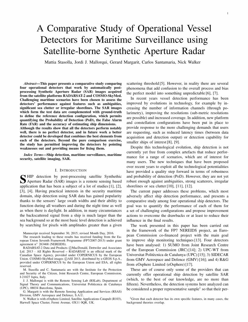
Fig. 9. CSK 20130606 045549: overview.

SUMO SIDECAR UPC-WT (R&G)

ND 10 6 9 -NF 60 16 5 -PoD 52.63% 31.58% 47.37% -FAR 1.52E-07 4.04E-08 1.26E-08 -

TABLE VICSK 20130606 045549: RESULTS.

As regards SIDECAR, we can notice that it has a low PoD(about 40%) and a higher FAR (about 6E-08).

Such high FAR is basically due to sea clutter: as clearlyshown by the strong red peak in Figure 8, almost allSIDECAR’s false alarms belong to the fourth group. Theremaining ones are instead associated to coastline inaccuracy.From the same histogram, we can also see that the issues forthe other detectors were different. SUMO was unable to masksome of the targets along the coast and, as well as UPC-WT,it did not properly handle large targets. With zero false alarms,R&G behaved well in all the situations.

3) CSK 20130606 045549: The third image is a single-look complex CSK HIMAGE product with a resolution of3×3 m. It was acquired over the Mediterranean sea off Lampe-dusa in June 2013. In this scene, which holds 19 targets,we can find all the challenging scenarios but sidelobes (seeFigure 9).

As reported in Table VI, the performances of all the threedetectors (as for the previous CSK image, R&G was not run)

0

5

10

15

20

25

30

35


SUMO

SIDECAR

UPC-WT

(R&G)

0

5

10

15

20

25

30


SUMO

SIDECAR

UPC-WT

R&G

0

10

20

30

40

50

60

70


SUMO

SIDECAR

UPC-WT

(R&G)

Fig. 10. CSK 20130606 045549: number of False Alarms VS challengingsituations.

8

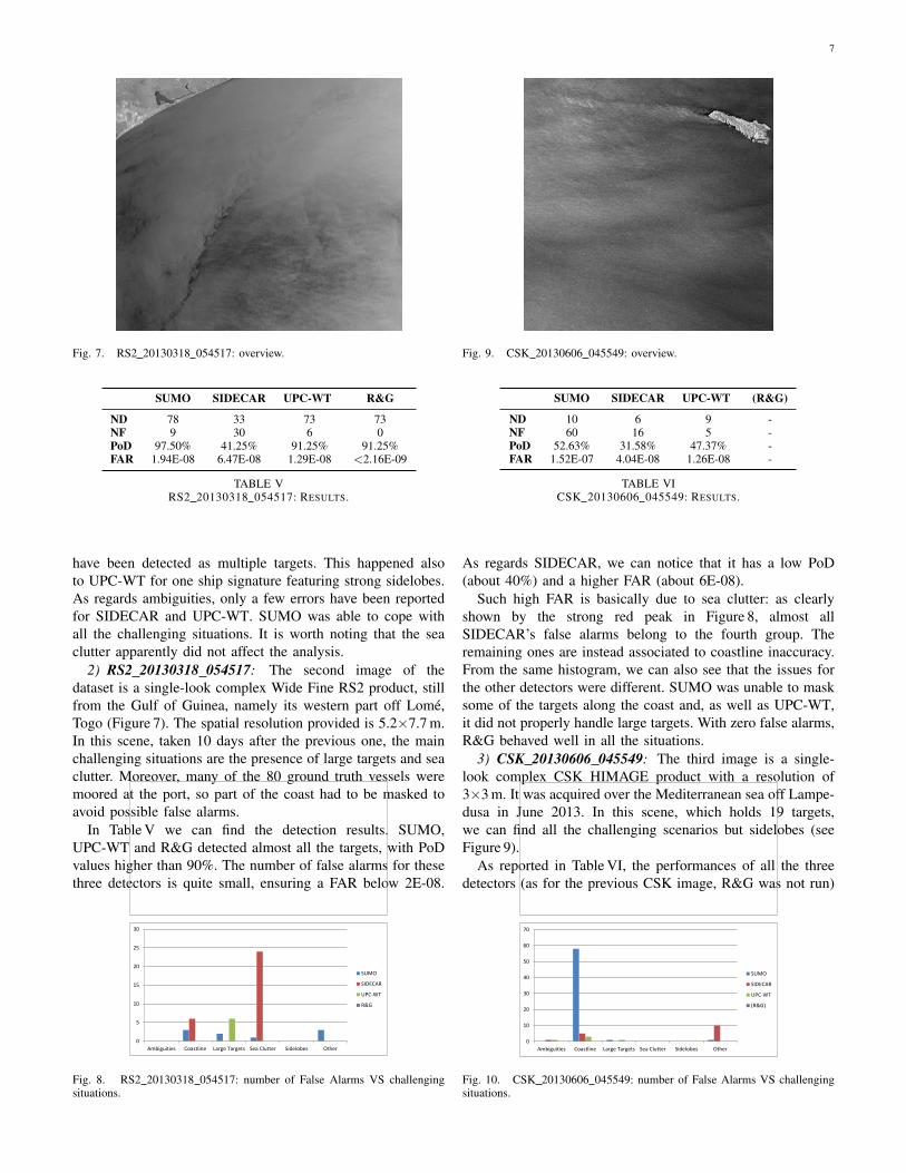
Fig. 11. RS2 20130606 050338: overview.


ND 26 11 18 9NF 8 8 10 1PoD 89.66% 37.93% 62.07% 31.03FAR 5.60E-08 5.60E-08 7.00E-08 7.00E-09

TABLE VIIRS2 20130606 050338: RESULTS.

are quite poor, with a maximum PoD of 52% reached bySUMO. Such a significant drop off of the detection accuracycan be explained considering that many of the vessels in thisarea were small fishing ships, which, due to their dimensions,were more difficult to be detected. As regards the false alarms,SUMO shows the highest number of errors, which caused aFAR of 1E-07. The other two detectors could reach a rateabout 10 times lower.

According to Figure 10, SUMO’s results were totally biasedby the large number of inland targets that were not filtered out.The reason is that the external land mask used to fit the actualcoastline was not sufficiently accurate in terms of both shapeand georeferentiation. In fact, SIDECAR and UPC-WT, thatare supplied with their own image-based coastline filters, couldsignificantly avoid this problem.

4) RS2 20130606 050338: The fourth image is again anacquisition from the area over the island of Lampedusa (Fig-ure 11), taken just a few minutes after the previous image. Theproduct is a single-look complex Standard RS2 image, with

0

1

2

3

4

5

6

7


SUMO

SIDECAR

UPC-WT

R&G

0

1

2

3

4

5

6

7

8


SUMO

SIDECAR

UPC-WT

R&G

0

10

20

30

40

50

60

70

80


SUMO

SIDECAR

UPC-WT

R&G*


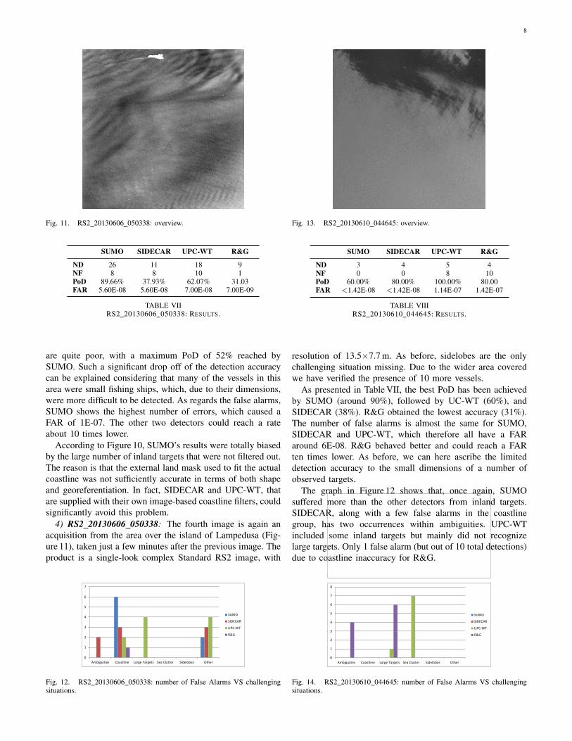
Fig. 13. RS2 20130610 044645: overview.


ND 3 4 5 4NF 0 0 8 10PoD 60.00% 80.00% 100.00% 80.00FAR <1.42E-08 <1.42E-08 1.14E-07 1.42E-07

TABLE VIIIRS2 20130610 044645: RESULTS.

resolution of 13.5×7.7 m. As before, sidelobes are the onlychallenging situation missing. Due to the wider area coveredwe have verified the presence of 10 more vessels.

As presented in Table VII, the best PoD has been achievedby SUMO (around 90%), followed by UC-WT (60%), andSIDECAR (38%). R&G obtained the lowest accuracy (31%).The number of false alarms is almost the same for SUMO,SIDECAR and UPC-WT, which therefore all have a FARaround 6E-08. R&G behaved better and could reach a FARten times lower. As before, we can here ascribe the limiteddetection accuracy to the small dimensions of a number ofobserved targets.

The graph in Figure 12 shows that, once again, SUMOsuffered more than the other detectors from inland targets.SIDECAR, along with a few false alarms in the coastlinegroup, has two occurrences within ambiguities. UPC-WTincluded some inland targets but mainly did not recognizelarge targets. Only 1 false alarm (but out of 10 total detections)due to coastline inaccuracy for R&G.

0

1

2

3

4

5

6

7


SUMO

SIDECAR

UPC-WT

R&G

0

1

2

3

4

5

6

7

8


SUMO

SIDECAR

UPC-WT

R&G

0

10

20

30

40

50

60

70

80


SUMO

SIDECAR

UPC-WT

R&G*


9

5) RS2 20130610 044645: The last image is a multi-look detected Standard RS2 product, with a resolution of26.8×24.7 m. The area spotted, shown in Figure 13, is locatedabout 200 Km West of Crete, and contains only 5 ships. Thedetectors had to cope with ambiguities, large targets, seaclutter, and sidelobes.

From the statistical point of view, missing even one singletarget in this image could bias significantly the results. This iswell explained in Table VIII, where we can see that SUMO hasa PoD of only 60%, as it did not detect two targets. SIDECARand R&G missed only one target, so their PoD is 80%. Thebest performance is carried out by UPC-WT, which detected100% of the targets. Looking at the false alarms, SUMO andSIDECAR have no wrong detections, while almost two thirdsof UPC-WT and R&G’s total detections are incorrect. Thisled to a FAR of about 1E-07.

More in detail (Figure 14), UPC-WT did not properly man-age the sea clutter, whereas R&G was hindered by ambiguitiesand extended targets.

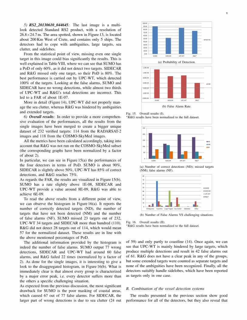
6) Overall results: In order to provide a more comprehen-sive evaluation of the performances, all the results from thesingle images have been merged to create a bigger uniquedataset of 232 verified targets: 114 from the RADARSAT-2images and 118 from the COSMO-SkyMed images.

All the metrics have been calculated accordingly, taking intoaccount that R&G was not run on the COSMO-SkyMed subset(the corresponding graphs have been normalized by a factorof about 2).In particular, we can see in Figure 15(a) the performances ofthe four detectors in terms of PoD. SUMO is about 90%,SIDECAR is slightly above 50%, UPC-WT has 85% of correctdetections, and R&G reaches 75%.As regards the FAR, the results are visualized in Figure 15(b).SUMO has a rate slightly above 1E-08, SIDECAR andUPC-WT provide a value around 8E-09, R&G was able toachieve 6E-09.

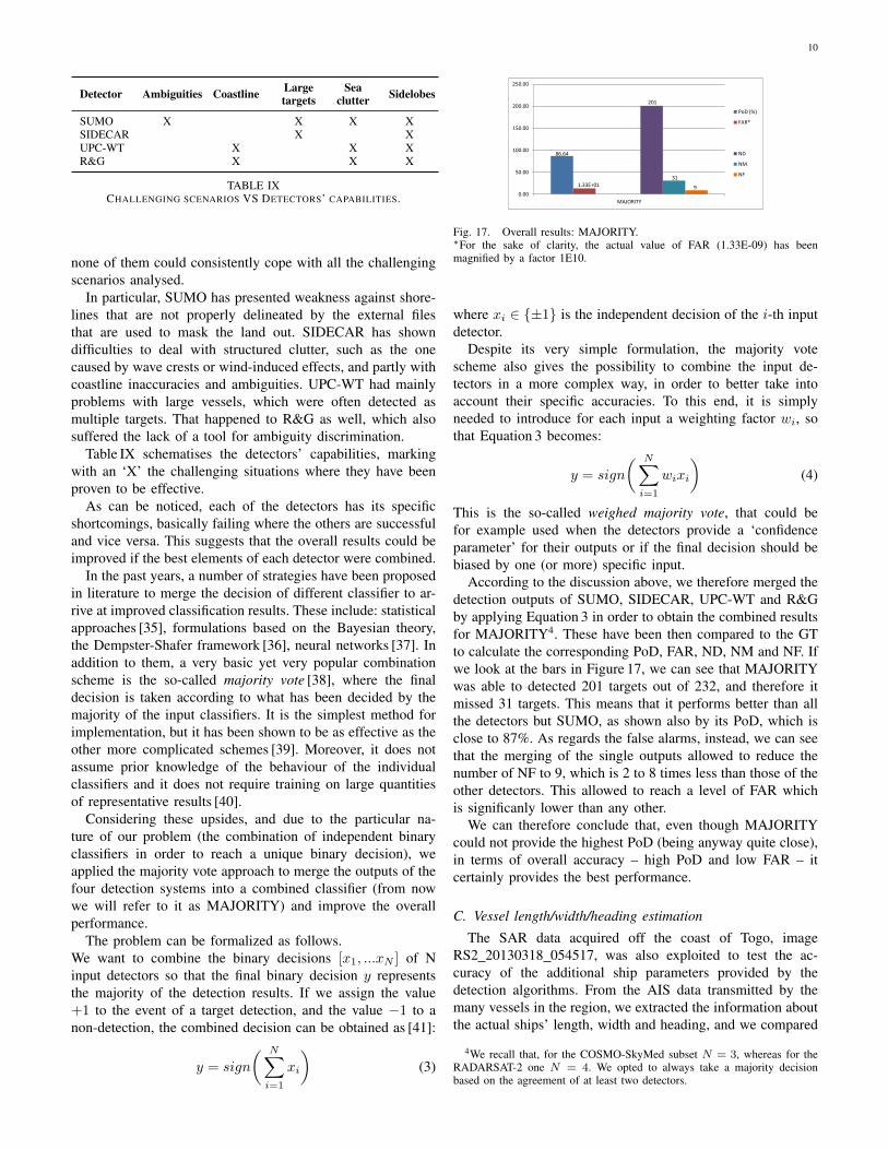
To read the above results from a different point of view,we can observe the histogram in Figure 16(a). It reports thenumber of correctly detected targets (ND), the number oftargets that have not been detected (NM) and the numberof false alarms (NF). SUMO missed 23 targets out of 232,UPC-WT 34 targets and SIDECAR more than hundred (110).R&G did not detect 28 targets out of 114, which would mean57 for the normalized dataset. These results are in line withthe above mentioned percentages of PoD.

The additional information provided by the histogram isindeed the number of false alarms. SUMO output 77 wrongdetections, SIDECAR and UPC-WT had around 60 falsealarms, and R&G failed 22 times (normalized by a factor of2). As done for the single images, it is interesting to give alook to the disaggregated histogram, in Figure 16(b). What isimmediately clear is that almost every group is characterizedby a major error peak, i.e. every detector suffers more thanthe others a specific challenging situation.As expected from the previous discussion, the most significantdrawback for SUMO is the poor masking of coastal areas,which caused 67 out of 77 false alarms. For SIDECAR, thelarger part of wrong detections is due to sea clutter (24 out

0.00

10.00

20.00

30.00

40.00

50.00

60.00

70.00

80.00

90.00

100.00

SUMO SIDECAR UPC-WT R&G*

PoD (%)

0.00E+00

2.00E-09

4.00E-09

6.00E-09

8.00E-09

1.00E-08

1.20E-08


FAR

0

50

100

150

200

250


ND

NM

NF

(a) Probability of Detection.

0.00

10.00

20.00

30.00

40.00

50.00

60.00

70.00

80.00

90.00

100.00


PoD (%)

0.00E+00

2.00E-09

4.00E-09

6.00E-09

8.00E-09

1.00E-08

1.20E-08


FAR

0

50

100

150

200

250


ND

NM

NF

(b) False Alarm Rate.

Fig. 15. Overall results (I).∗R&G results have been normalized to the full dataset.

0.00

10.00

20.00

30.00

40.00

50.00

60.00

70.00

80.00

90.00

100.00


PoD (%)

0.00E+00

2.00E-09

4.00E-09

6.00E-09

8.00E-09

1.00E-08

1.20E-08


FAR

0

50

100

150

200

250


ND

NM

NF

(a) Number of correct detections (ND); missed targets(NM); false alarms (NF).

0

10

20

30

40

50

60

70

80


SUMO

SIDECAR

UPC-WT

R&G*

(b) Number of False Alarms VS challenging situations.

Fig. 16. Overall results (II).∗R&G results have been normalized to the full dataset.

of 59) and only partly to coastline (14). Once again, we cansee that UPC-WT is mainly hindered by large targets, whichproduce multiple detections and result in 42 false alarms outof 61. R&G does not have a clear peak in any of the groups,but some extended targets were counted as separate targets andnone of the ambiguities have been recognized. Finally, all thedetectors suitably handle sidelobes, which have been reportedas targets only in one case.

B. Combination of the vessel detection systems

The results presented in the previous section show goodperformance for all of the detectors, but they also reveal that

10

Detector Ambiguities Coastline Largetargets

Seaclutter Sidelobes

SUMO X X X XSIDECAR X XUPC-WT X X XR&G X X X

TABLE IXCHALLENGING SCENARIOS VS DETECTORS’ CAPABILITIES.

none of them could consistently cope with all the challengingscenarios analysed.

In particular, SUMO has presented weakness against shore-lines that are not properly delineated by the external filesthat are used to mask the land out. SIDECAR has showndifficulties to deal with structured clutter, such as the onecaused by wave crests or wind-induced effects, and partly withcoastline inaccuracies and ambiguities. UPC-WT had mainlyproblems with large vessels, which were often detected asmultiple targets. That happened to R&G as well, which alsosuffered the lack of a tool for ambiguity discrimination.

Table IX schematises the detectors’ capabilities, markingwith an ‘X’ the challenging situations where they have beenproven to be effective.

As can be noticed, each of the detectors has its specificshortcomings, basically failing where the others are successfuland vice versa. This suggests that the overall results could beimproved if the best elements of each detector were combined.

In the past years, a number of strategies have been proposedin literature to merge the decision of different classifier to ar-rive at improved classification results. These include: statisticalapproaches [35], formulations based on the Bayesian theory,the Dempster-Shafer framework [36], neural networks [37]. Inaddition to them, a very basic yet very popular combinationscheme is the so-called majority vote [38], where the finaldecision is taken according to what has been decided by themajority of the input classifiers. It is the simplest method forimplementation, but it has been shown to be as effective as theother more complicated schemes [39]. Moreover, it does notassume prior knowledge of the behaviour of the individualclassifiers and it does not require training on large quantitiesof representative results [40].

Considering these upsides, and due to the particular na-ture of our problem (the combination of independent binaryclassifiers in order to reach a unique binary decision), weapplied the majority vote approach to merge the outputs of thefour detection systems into a combined classifier (from nowwe will refer to it as MAJORITY) and improve the overallperformance.

The problem can be formalized as follows.We want to combine the binary decisions [x1, ...xN ] of Ninput detectors so that the final binary decision y representsthe majority of the detection results. If we assign the value+1 to the event of a target detection, and the value −1 to anon-detection, the combined decision can be obtained as [41]:

y = sign

( N∑i=1

xi

)(3)

86.64

1.33E+01

201

31

9 0.00

50.00

100.00

150.00

200.00

250.00

MAJORITY

PoD (%)

FAR*

Series3

Series4

ND

NM

NF

84.87

-1.31

2.45E+00

-1.61E+01

129

-2

23

2

9

-59 -65

-15

35

85

135

SUMO

PoD (%)

FAR*

ND

NM

NF

Difference

Fig. 17. Overall results: MAJORITY.∗For the sake of clarity, the actual value of FAR (1.33E-09) has beenmagnified by a factor 1E10.

where xi ∈ {±1} is the independent decision of the i-th inputdetector.

Despite its very simple formulation, the majority votescheme also gives the possibility to combine the input de-tectors in a more complex way, in order to better take intoaccount their specific accuracies. To this end, it is simplyneeded to introduce for each input a weighting factor wi, sothat Equation 3 becomes:

y = sign

( N∑i=1

wixi

)(4)

This is the so-called weighed majority vote, that could befor example used when the detectors provide a ‘confidenceparameter’ for their outputs or if the final decision should bebiased by one (or more) specific input.

According to the discussion above, we therefore merged thedetection outputs of SUMO, SIDECAR, UPC-WT and R&Gby applying Equation 3 in order to obtain the combined resultsfor MAJORITY4. These have been then compared to the GTto calculate the corresponding PoD, FAR, ND, NM and NF. Ifwe look at the bars in Figure 17, we can see that MAJORITYwas able to detected 201 targets out of 232, and therefore itmissed 31 targets. This means that it performs better than allthe detectors but SUMO, as shown also by its PoD, which isclose to 87%. As regards the false alarms, instead, we can seethat the merging of the single outputs allowed to reduce thenumber of NF to 9, which is 2 to 8 times less than those of theother detectors. This allowed to reach a level of FAR whichis significanly lower than any other.

We can therefore conclude that, even though MAJORITYcould not provide the highest PoD (being anyway quite close),in terms of overall accuracy – high PoD and low FAR – itcertainly provides the best performance.

C. Vessel length/width/heading estimation

The SAR data acquired off the coast of Togo, imageRS2 20130318 054517, was also exploited to test the ac-curacy of the additional ship parameters provided by thedetection algorithms. From the AIS data transmitted by themany vessels in the region, we extracted the information aboutthe actual ships’ length, width and heading, and we compared

4We recall that, for the COSMO-SkyMed subset N = 3, whereas for theRADARSAT-2 one N = 4. We opted to always take a majority decisionbased on the agreement of at least two detectors.

11

AIS SUMO UPC-WT R&G

# of detections 70 78 73 73# of correlated targets 63# of reliable targets 59

Average length difference [m] -28.83 41.50 24.66

Average length difference (absolute) [m] 46.44 47.00 31.73

Average width difference [m] 2.12 48.27 12.44

Average width difference (absolute) [m] 10.51 48.27 14.80

TABLE XRS2 20130318 054517: LENGTH/WIDTH ESTIMATION.

(a) Overall detections.

(b) Focussing on one vessel as reportedby AIS (ATLANTIS ANTIBES) and de-tected by SUMO (j24), UPC-WT (u44)and R&G (e39).

Fig. 18. RS2 20130318 054517: Detection results. The vessels are displayedas arrows, oriented according to the reported or detected heading and thelength of each arrow is proportional to the reported or detected vessel length.

them against the estimations from SUMO, UPC-WT and R&G(GMV results were not available).Figure 18(a) shows an overview of all the detections togetherwith the results from the AIS data. The vessels are displayed asarrows, oriented according to the reported or detected headingand the length of each arrow is proportional to the reportedor detected vessel length.The number of recorded detections for the AIS system andfor each of the algorithms is shown in Table X. It can be seenthat the number of AIS-transmitting ships and the number ofdetections for each of the algorithms are fairly similar. Only70 out of 80 verified targets transmitted AIS signals.Figure 18(b) shows the result of focussing on one vessel, theAtlantis Antibes, as reported by AIS and detected by SUMO,UPC-WT and R&G.

Of the 70 vessels reported by the AIS, there were 63 whichwere also detected by all three SUMO, UPC-WT and R&G.Of these 63 sets of data it was found that 4 were missing

R² = 0.2864

R² = 0.5666 R² = 0.53

0

100

200

300

0 100 200 300 400 500

AIS

Ve

sse

l Le

ngt

h (

m)

Detected Vessel Length (m)

SUMO

UPC-WT

R&G

Linear (SUMO)

Linear (UPC-WT)

Linear (R&G)

R² = 0.1717 R² = 0.4641 R² = 0.1212

0

50

100

0 50 100 150

AIS

Ve

sse

l Wid

th (

m)

Detected Vessel Width (m)

SUMO

UPC

eOsphere

Linear (SUMO)

Linear (UPC)

Linear (eOsphere)

0

5

10

15

20

25

30

3530

60

90

120

150

180

210

240

270

300

330

360

SUMO

UPC-WT

R&G

AIS

(a) Reported AIS vessels lengths VS algorithm detectedvessel lengths.

R² = 0.2864

R² = 0.5666 R² = 0.53

0

100

200

300

0 100 200 300 400 500

AIS

Ve

sse

l Le

ngt

h (

m)


SUMO

UPC-WT

R&G

Linear (SUMO)

Linear (UPC-WT)

Linear (R&G)

R² = 0.1717 R² = 0.4641 R² = 0.1212

0

50

100

0 50 100 150

AIS

Ve

sse

l Wid

th (

m)


SUMO

UPC

eOsphere

Linear (SUMO)

Linear (UPC)

Linear (eOsphere)

0

5

10

15

20

25

30

3530

60

90

120

150

180

210

240

270

300

330

360

SUMO

UPC-WT

R&G

AIS

(b) Reported AIS vessels widths VS algorithm detectedvessel widths.

Fig. 19. RS2 20130318 054517: Length/width estimation.

some information from their AIS reports (usually the vesseldimensions), which made them unusable in the analysis.This left 59 data sets to be included in the analysis wherethere was simultaneously an AIS report and detections fromall three algorithms.

1) Vessel length: Figure 19(a) shows a scatterplot for the59 AIS reports for the vessel lengths, versus the vessel lengthsas measured by the three different algorithms. It can be seenthat there is a degree of correlation between the reported anddetected vessel lengths; however if it is assumed that the AISreported lengths are relatively accurate, then there is a degreeof error from each of the algorithms.

Table X shows, for each of the three algorithms, the meandifference between the AIS reported vessel lengths and thedetected vessel lengths and also the mean of the absolutedifference between the AIS reported vessel lengths and thedetected vessel lengths.

The fact that the average length differences between AISand the algorithm are positive for UPC-WT and R&G showsthat these algorithms, in general, are overestimating the vessellengths. This tendency can be observed in the scatterplot in

12

Figure 19(a), where the linear regression lines for these twoalgorithms are below the 45 degree diagonal line that wouldrepresent equal values of AIS and algorithm length.

In contrast, SUMO has a negative average length differ-ence between itself and the AIS data, which indicates that,on average, it is underestimating the vessel lengths. FromFigure 19(a) it can be seen that this tendency to underestimatevessel lengths is more pronounced at smaller vessel sizes, butthat the estimates become more accurate for larger vessels.

The mean of the absolute differences between the AISreported vessel lengths and the detected vessel lengths, shownstill in Table X, give an overall summary of how accurate thedetection algorithms are. It can be seen that R&G provides themost accurate results and that the mean of the averages of theabsolute differences is 41.72 m, which indicates that there isroom for improvement, especially because the average valueof the reported AIS vessel lengths is 138.87 and therefore anerror of 41.72 m represents a percentage of 30%.

2) Vessel width: Figure 19(b) shows a scatterplot for the59 AIS reports for the vessel widths, versus the vessel widthsas measured by the three different algorithms.

Table X shows, for each of the three algorithms, the meandifference between the AIS reported vessel widths and thedetected vessel widths and also the mean of the absolutedifference between the AIS reported vessel widths and thedetected vessel widths.

It can be seen that all three algorithms are, on average,providing overestimates of the vessel widths, however, SUMOhas a very low average, indicating that, in general, it isunderestimating almost as often as overestimating. The meansof the absolute differences provide an overall measure ofthe performance, where it can be seen that SUMO is themost accurate, followed by R&G, with the UPC-WT fallingsignificantly behind.

The average absolute error for the three algorithms is24.52 m, which, in fact, is greater than the average value ofthe vessel widths, 23.97 m, as reported by the AIS.

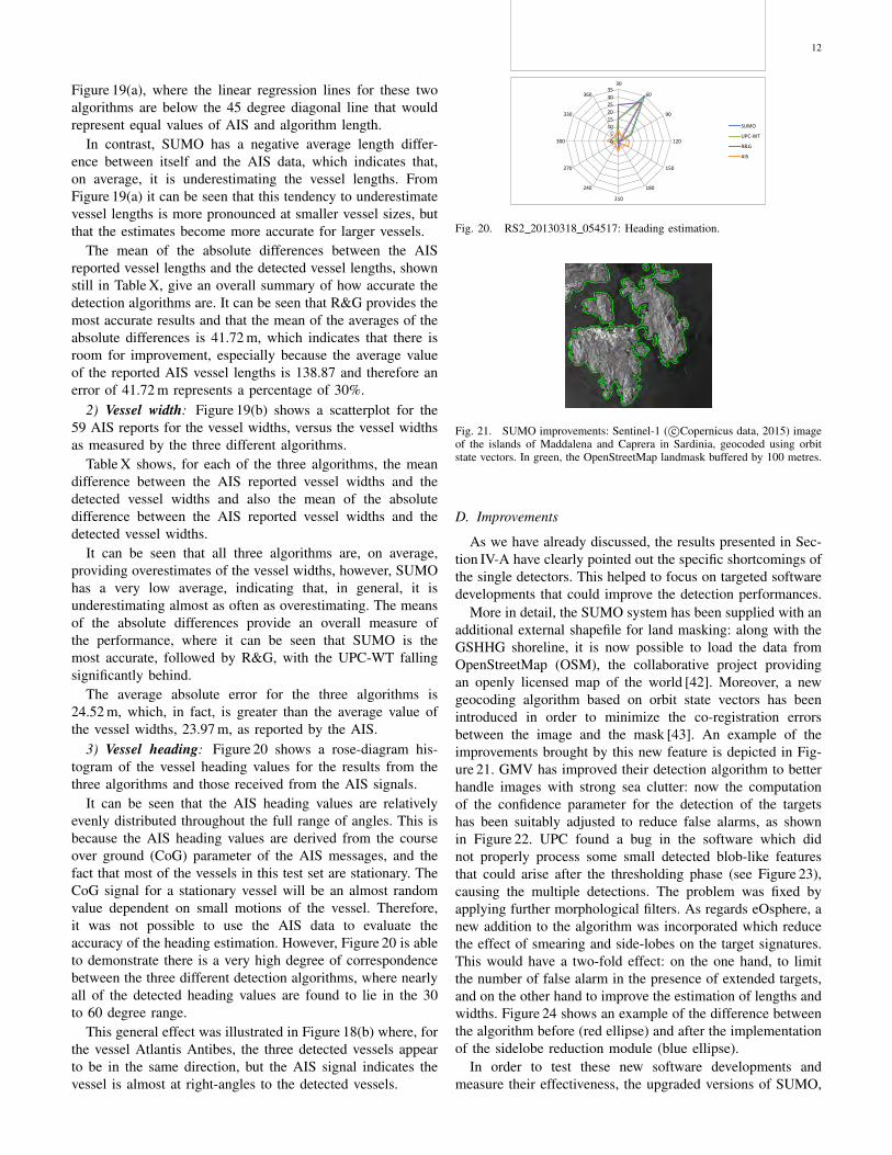
3) Vessel heading: Figure 20 shows a rose-diagram his-togram of the vessel heading values for the results from thethree algorithms and those received from the AIS signals.

It can be seen that the AIS heading values are relativelyevenly distributed throughout the full range of angles. This isbecause the AIS heading values are derived from the courseover ground (CoG) parameter of the AIS messages, and thefact that most of the vessels in this test set are stationary. TheCoG signal for a stationary vessel will be an almost randomvalue dependent on small motions of the vessel. Therefore,it was not possible to use the AIS data to evaluate theaccuracy of the heading estimation. However, Figure 20 is ableto demonstrate there is a very high degree of correspondencebetween the three different detection algorithms, where nearlyall of the detected heading values are found to lie in the 30to 60 degree range.

This general effect was illustrated in Figure 18(b) where, forthe vessel Atlantis Antibes, the three detected vessels appearto be in the same direction, but the AIS signal indicates thevessel is almost at right-angles to the detected vessels.

0

100

200

300

0 100 200 300 400 500

AIS

Ve

sse

l Le

ngt

h (

m)


SUMO

UPC-WT

R&G

Linear (SUMO)

Linear (UPC-WT)

Linear (R&G)

0

50

100

0 50 100 150

AIS

Ve

sse

l Wid

th (

m)


SUMO

UPC

eOsphere

Linear (SUMO)

Linear (UPC)

Linear (eOsphere)

0

5

10

15

20

25

30

3530

60

90

120

150

180

210

240

270

300

330

360

SUMO

UPC-WT

R&G

AIS

Fig. 20. RS2 20130318 054517: Heading estimation.

Fig. 21. SUMO improvements: Sentinel-1 ( c©Copernicus data, 2015) imageof the islands of Maddalena and Caprera in Sardinia, geocoded using orbitstate vectors. In green, the OpenStreetMap landmask buffered by 100 metres.

D. Improvements

As we have already discussed, the results presented in Sec-tion IV-A have clearly pointed out the specific shortcomings ofthe single detectors. This helped to focus on targeted softwaredevelopments that could improve the detection performances.

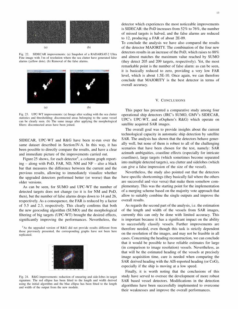
More in detail, the SUMO system has been supplied with anadditional external shapefile for land masking: along with theGSHHG shoreline, it is now possible to load the data fromOpenStreetMap (OSM), the collaborative project providingan openly licensed map of the world [42]. Moreover, a newgeocoding algorithm based on orbit state vectors has beenintroduced in order to minimize the co-registration errorsbetween the image and the mask [43]. An example of theimprovements brought by this new feature is depicted in Fig-ure 21. GMV has improved their detection algorithm to betterhandle images with strong sea clutter: now the computationof the confidence parameter for the detection of the targetshas been suitably adjusted to reduce false alarms, as shownin Figure 22. UPC found a bug in the software which didnot properly process some small detected blob-like featuresthat could arise after the thresholding phase (see Figure 23),causing the multiple detections. The problem was fixed byapplying further morphological filters. As regards eOsphere, anew addition to the algorithm was incorporated which reducethe effect of smearing and side-lobes on the target signatures.This would have a two-fold effect: on the one hand, to limitthe number of false alarm in the presence of extended targets,and on the other hand to improve the estimation of lengths andwidths. Figure 24 shows an example of the difference betweenthe algorithm before (red ellipse) and after the implementationof the sidelobe reduction module (blue ellipse).

In order to test these new software developments andmeasure their effectiveness, the upgraded versions of SUMO,

13

(a) (b)

Fig. 22. SIDECAR improvements: (a) Snapshot of a RADARSAT-2 UltraFine image with 3 m of resolution where the sea clutter have generated falsealarms (yellow dots). (b) Removal of the false alarms.

(a) (b)

Fig. 23. UPC-WT improvements: (a) Image after scaling with the sea clutterstatistics and thresholding: disconnected areas belonging to the same vesselcan be clearly seen. (b) The same image after applying the morphologicalfilters: disconnected areas have been joined.

SIDECAR, UPC-WT and R&G have been re-run over thesame dataset described in Section IV-A. In this way, it hasbeen possible to directly compare the results, and have a clearand immediate picture of the improvements carried out.

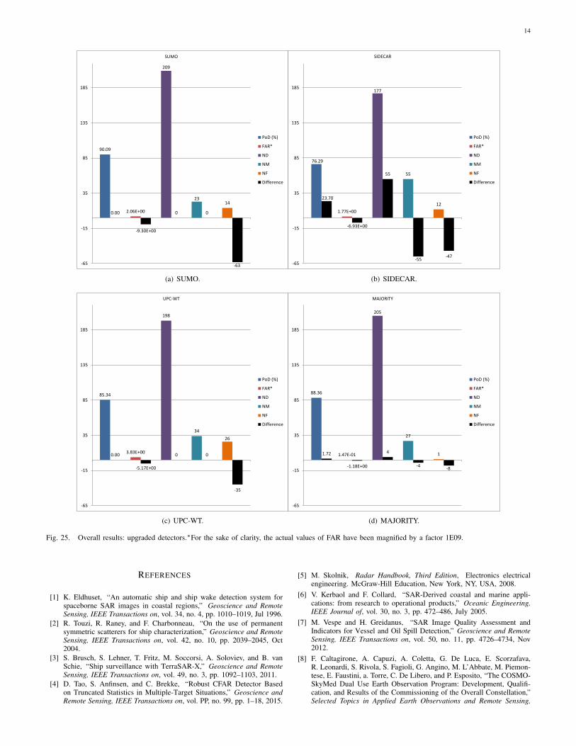
Figure 25 shows, for each detector5, a column graph report-ing – along with PoD, FAR, ND, NM and NF – also a blackbar that measures the difference between the current and theprevious results, allowing to immediately visualize whetherthe upgraded detectors performed better (or worse) than theolder versions.

As can be seen, for SUMO and UPC-WT the number ofdetected targets does not change (so it is for NM and PoD,then), but the number of false alarms drops down to 14 and 26,respectively. As a consequence, the FAR is reduced by a factorof 5.5 and 2.3, respectively. This clearly confirms that boththe new geocoding algorithm (SUMO) and the morphologicalfiltering of big targets (UPC-WT) brought the desired effects,significantly improving the performances. Nevertheless, the

5As the upgraded version of R&G did not provide results different fromthose previously presented, the corresponding graphs have not been herereplicated.

Fig. 24. R&G improvements: reduction of smearing and side-lobes in targetsignature. The red ellipse has been fitted to the length and width derivedusing the initial algorithm and the blue ellipse has been fitted to the lengthand width of the output from the new module.

detector which experiences the most noticeable improvementsis SIDECAR: the PoD increases from 52% to 76%, the numberof missed targets is halved, and the false alarms are reducedto 12, producing a FAR of about 2E-09.To conclude the analysis we have also compared the resultsof the detector MAJORITY. The combination of the four newdetectors results in an increase of the PoD, which raises to 88%and almost matches the maximum value reached by SUMO(they detect 205 and 209 targets, respectively). Yet, the mostremarkable point is the number of false alarm: as can be seen,it is basically reduced to zero, providing a very low FARlevel, which is about 1.5E-10. Once again, we can thereforeconclude that MAJORITY is the best detector in terms ofoverall accuracy.

V. CONCLUSIONS

This paper has presented a comparative study among fouroperational ship detectors (JRC’s SUMO, GMV’s SIDECAR,UPC’s UPC-WT, and eOsphere’s R&G) which operate onsatellite acquired SAR images.

The overall goal was to provide insights about the currenttechnological capacity in automatic ship detection by satelliteSAR. The analysis has shown that the detectors behave gener-ally well, but none of them is robust to all of the challengingscenarios that have been chosen for the test, namely: SARazimuth ambiguities, coastline effects (especially for intricatecoastlines), large targets (which sometimes become separatedinto multiple detected targets), sea clutter and sidelobes (whichcan give a false impression of the size of the vessel).

Nevertheless, the study also pointed out that the detectorshave specific shortcomings (they basically fail where the othersare successful and vice versa) that make them somehow com-plementary. This was the starting point for the implementationof a merging scheme based on the majority vote approach thatallow to suitably combine the single outputs and improve theoverall results.

As regards the second part of the analysis, i.e. the estimationof the length and width of the vessels from SAR images,currently this can only be done with limited accuracy. Thisis important because it has a significant impact on the abilityto successfully classify vessels. Further improvements aretherefore needed, even though this task is strictly dependenton the resolution of the images, and may not be feasible in allcases. Concerning the heading reconstruction, we can concludethat it would be possible to have reliable estimates for large(in comparison to image resolution) vessels. Nevertheless, asthat will be the estimated heading of the vessels at preciselyimage acquisition time, care is needed when comparing theSAR derived heading with the AIS-reported heading (or CoG),especially if the ship is moving at a low speed.

Finally, it is worth noting that the conclusions of thisstudy have served to oversee the development of more robustSAR based vessel detectors. Modifications in the detectionalgorithms have been successfully implemented to overcometheir weaknesses and improve the overall performances.

14

90.09

0.00 2.06E+00

-9.30E+00

209

0

23

0

14

-63 -65

-15

35

85

135

185

SUMO

PoD (%)

FAR*

ND

NM

NF

Difference

(a) SUMO.

76.29

23.70

1.77E+00

-6.93E+00

177

55 55

-55

12

-47

-65

-15

35

85

135

185

SIDECAR

PoD (%)

FAR*

ND

NM

NF

Difference

(b) SIDECAR.

85.34

0.00 3.83E+00

-5.17E+00

198

0

34

0

26

-35

-65

-15

35

85

135

185

UPC-WT

PoD (%)

FAR*

ND

NM

NF

Difference

(c) UPC-WT.

88.36

1.72 1.47E-01

-1.18E+00

205

4

27

-4

1

-8

-65

-15

35

85

135

185

MAJORITY

PoD (%)

FAR*

ND

NM

NF

Difference

(d) MAJORITY.

Fig. 25. Overall results: upgraded detectors.∗For the sake of clarity, the actual values of FAR have been magnified by a factor 1E09.

REFERENCES

[1] K. Eldhuset, “An automatic ship and ship wake detection system forspaceborne SAR images in coastal regions,” Geoscience and RemoteSensing, IEEE Transactions on, vol. 34, no. 4, pp. 1010–1019, Jul 1996.

[2] R. Touzi, R. Raney, and F. Charbonneau, “On the use of permanentsymmetric scatterers for ship characterization,” Geoscience and RemoteSensing, IEEE Transactions on, vol. 42, no. 10, pp. 2039–2045, Oct2004.

[3] S. Brusch, S. Lehner, T. Fritz, M. Soccorsi, A. Soloviev, and B. vanSchie, “Ship surveillance with TerraSAR-X,” Geoscience and RemoteSensing, IEEE Transactions on, vol. 49, no. 3, pp. 1092–1103, 2011.

[4] D. Tao, S. Anfinsen, and C. Brekke, “Robust CFAR Detector Basedon Truncated Statistics in Multiple-Target Situations,” Geoscience andRemote Sensing, IEEE Transactions on, vol. PP, no. 99, pp. 1–18, 2015.

[5] M. Skolnik, Radar Handbook, Third Edition, Electronics electricalengineering. McGraw-Hill Education, New York, NY, USA, 2008.

[6] V. Kerbaol and F. Collard, “SAR-Derived coastal and marine appli-cations: from research to operational products,” Oceanic Engineering,IEEE Journal of, vol. 30, no. 3, pp. 472–486, July 2005.

[7] M. Vespe and H. Greidanus, “SAR Image Quality Assessment andIndicators for Vessel and Oil Spill Detection,” Geoscience and RemoteSensing, IEEE Transactions on, vol. 50, no. 11, pp. 4726–4734, Nov2012.

[8] F. Caltagirone, A. Capuzi, A. Coletta, G. De Luca, E. Scorzafava,R. Leonardi, S. Rivola, S. Fagioli, G. Angino, M. L’Abbate, M. Piemon-tese, E. Faustini, a. Torre, C. De Libero, and P. Esposito, “The COSMO-SkyMed Dual Use Earth Observation Program: Development, Qualifi-cation, and Results of the Commissioning of the Overall Constellation,”Selected Topics in Applied Earth Observations and Remote Sensing,

15

IEEE Journal of, vol. 7, no. 7, pp. 2754–2762, July 2014.[9] R. Torres, P. Snoeij, D. Geudtner, D. Bibby, M. Davidson, E. Attema,

P. Potin, B. Rommen, N. Floury, M. Brown, et al., “GMES Sentinel-1mission,” Remote Sensing of Environment, vol. 120, pp. 9–24, 2012.

[10] G. Di Martino, A. Iodice, D. Riccio, and G. Ruello, “Filtering ofAzimuth Ambiguity in Stripmap Synthetic Aperture Radar Images,”Selected Topics in Applied Earth Observations and Remote Sensing,IEEE Journal of, vol. 7, no. 9, pp. 3967–3978, Sept 2014.

[11] A. Buono, F. Nunziata, L. Mascolo, and M. Migliaccio, “A Multi-polarization Analysis of Coastline Extraction Using X-Band COSMO-SkyMed SAR Data,” Selected Topics in Applied Earth Observations andRemote Sensing, IEEE Journal of, vol. 7, no. 7, pp. 2811–2820, July2014.

[12] X. Zhao, Y. Jiang, and W.-Q. Wang, “Efficient Clutter Suppressionin SAR Images With Shedding Irrelevant Patterns,” Geoscience andRemote Sensing Letters, IEEE, vol. 12, no. 9, pp. 1828–1832, Sept 2015.

[13] www.cordis.europa.eu/project/rcn/99070 en, accessed March 10, 2016.[14] N. Kourti, I. Shepherd, G. Schwartz, and P. Pavlakis, “Integrating Space-

borne SAR Imagery into Operational Systems for Fisheries Monitoring,”Canadian Journal of Remote Sensing, vol. 27, no. 4, pp. 291–305, 2001.

[15] M. Tello, C. Lopez-Martinez, and J. Mallorqui, “A novel algorithmfor ship detection in SAR imagery based on the wavelet transform,”Geoscience and Remote Sensing Letters, IEEE, vol. 2, no. 2, pp. 201–205, April 2005.

[16] G. Margarit, J. A. Barba Milans, and A. Tabasco, “Operational ShipMonitoring System Based on Synthetic Aperture Radar Processing,”Remote Sensing, vol. 1, no. 3, pp. 375, 2009.

[17] A. Marino, N. Walker, and I. Hajnsek, “Perturbation analysis formaritime applications,” in Synthetic Aperture Radar, 2012. EUSAR. 9thEuropean Conference on, April 2012, pp. 509–512.

[18] H. Greidanus, “Vessel Classification Benchmark,” Tech. Rep. DECLIMSD4, European Commission - Joint Research Centre, 2007.

[19] B. Venners, Inside the Java Virtual Machine, McGraw-Hill Professional,New York, NY, USA, 1st edition, 1999.

[20] C. Oliver and S. Quegan, Understanding Synthetic Aperture RadarImages, SciTech Publ., Raleigh, NC, USA, 2004.

[21] P. Wessel and W. H. Smith, “A global, self-consistent, hierarchical,high-resolution shoreline database,” Journal of Geophysical Research:Solid Earth (1978–2012), vol. 101, no. B4, pp. 8741–8743, 1996.

[22] M. Tello, C. Lopez-Martinez, and J. J. Mallorqui, “Automatic vesselmonitoring with single and multidimensional SAR images in the waveletdomain,” ISPRS Journal of Photogrammetry and Remote Sensing, vol.61, no. 34, pp. 260 – 278, 2006.

[23] R. Haralick, S. R. Sternberg, and X. Zhuang, “Image Analysis UsingMathematical Morphology,” Pattern Analysis and Machine Intelligence,IEEE Transactions on, vol. PAMI-9, no. 4, pp. 532–550, July 1987.

[24] T. Xiong, S. Wang, B. Hou, Y. Wang, and H. Liu, “A Resample-BasedSVA Algorithm for Sidelobe Reduction of SAR/ISAR Imagery WithNoninteger Nyquist Sampling Rate,” Geoscience and Remote Sensing,IEEE Transactions on, vol. 53, no. 2, pp. 1016–1028, Feb 2015.

[25] M. Tello Alonso, C. Lopez-Martinez, J. Mallorqui, and P. Salembier,“Edge Enhancement Algorithm Based on the Wavelet Transform forAutomatic Edge Detection in SAR Images,” Geoscience and RemoteSensing, IEEE Transactions on, vol. 49, no. 1, pp. 222–235, Jan 2011.

[26] International Maritime Organization, Automatic Identifcation Systems,Model course. International Maritime Organization, 2006.

[27] S. Mallat, A wavelet tour of signal processing, AcademicP ress,Burlington, MA, USA, 1999.

[28] V. Caselles, R. Kimmel, and G. Sapiro, “Geodesic active contours,”International journal of computer vision, vol. 22, no. 1, pp. 61–79, 1997.

[29] M. Kass, A. Witkin, and D. Terzopoulos, “Snakes: Active contourmodels,” International journal of computer vision, vol. 1, no. 4, pp.321–331, 1988.

[30] K. Tanaka, An introduction to fuzzy logic for practical applications,Springer-Verlag, New York, NY, USA, 1997.

[31] P. Soille, Morphological Image Analysis: Principles and Applications,Springer-Verlag New York, Inc., Secaucus, NJ, USA, 2 edition, 2003.

[32] A. Freeman, “On ambiguities in SAR design,” Synthetic Aperture Radar,2006. EUSAR. 6th European Conference on, May 2006.

[33] P. D. Mourad, “Footprints of Atmospheric Phenomena in SyntheticAperture Radar Images of the Ocean Surface: A Review,” in Air-SeaExchange: Physics, Chemistry and Dynamics, G. L. Geernaert, Ed., pp.269–290. Springer Netherlands, Dordrecht, The Netherlands, 1999.

[34] B. Smith, “An analytic nonlinear approach to sidelobe reduction,” ImageProcessing, IEEE Transactions on, vol. 10, no. 8, pp. 1162–1168, Aug2001.

[35] Y. Shiraishi and K. Fukumizu, “Statistical approaches to combiningbinary classifiers for multi-class classification,” Neurocomputing, vol.74, no. 5, pp. 680 – 688, 2011.

[36] B. Quost, M.-H. Masson, and T. Denœux, “Classifier fusion in theDempster–Shafer framework using optimized t-norm based combinationrules,” International Journal of Approximate Reasoning, vol. 52, no. 3,pp. 353 – 374, 2011.

[37] X. Li, L. Wang, and E. Sung, “Adaboost with SVM-based componentclassifiers,” Eng. Appl. Artif. Intell., vol. 21, no. 5, pp. 785–795, Aug.2008.

[38] L. I. Kuncheva, Combining Pattern Classifiers: Methods and Algorithms,Wiley-Interscience, Hoboken, NJ, USA, 2004.

[39] D. Lee and S. Srihari, “Handprinted digit recognition: a comparison ofalgorithms,” in Proceedings of the 3rd International Workshop FrontiersHandwriting Recognition, 1993.

[40] L. Lam and C. Y. Suen, “Application of majority voting to patternrecognition: an analysis of its behavior and performance,” IEEETransactions on Systems, Man, and Cybernetics - Part A: Systems andHumans, vol. 27, no. 5, pp. 553–568, Sep 1997.

[41] D. Berend and A. Kontorovitch, “Consistency of weighted majorityvotes,” in Advances in Neural Information Processing Systems 27,Z. Ghahramani, M. Welling, C. Cortes, N. Lawrence, and K. Weinberger,Eds., pp. 3446–3454. Curran Associates, Inc., 2014.

[42] M. Haklay and P. Weber, “OpenStreetMap: User-Generated StreetMaps,” Pervasive Computing, IEEE, vol. 7, no. 4, pp. 12–18, Oct 2008.

[43] G. Schreier, SAR Geocoding: Data and Systems, Wichmann, Karlsruhe,Germany, 1993.

Documents

A Comparative Study of Operational Vessel Detectors for