A Commodity Curse?

The Dynamic Effects of Commodity Prices on Fiscal Performance in

Latin America

Leandro Medina1

Version: January 2010

Abstract

The recent boom and bust in commodity prices has raised concerns about the impact of volatile commodity prices on Latin American countries’ fiscal positions. Using a novel quarterly dataset─ which includes unique country specific commodity price indices and a comprehensive measure of public expenditures─ this paper analyzes the dynamic effects of commodity price fluctuations on fiscal revenues and expenditures for 8 commodity exporting Latin American countries. The results indicate that Latin American countries’ fiscal positions generally react strongly to shocks to commodity prices, yet there are marked differences across countries in observed reactions. Fiscal variables in Venezuela display the highest sensitivity to commodity price shocks, with expenditures reacting significantly more than revenues. On the other side of the spectrum, Chile’s fiscal indicators react very little to commodity price fluctuations, and their dynamic responses are very similar to those seen in high-income commodity exporting countries. A plausible explanation to this distinct behavior across countries could be related to the efficient application of fiscal rules, accompanied by strong institutions, political commitment and high standards of transparency.

1 Ph. D. Candidate, The George Washington University, Department of Economics. Email: leandrom@gwmail.gwu.edu. Financial support from the CAF is gratefully acknowledged. The author wishes to thank the helpful comments of Adriana Arreaza, Ana Corbacho, Gabriel Di Bella, Fred Joutz, Herman Kamil, Graciela Kaminsky, Tara Sinclair, Antonio Spilimbergo and participants at LACEA 2009 Conference held in Buenos Aires, Argentina. Special thanks to Carlos Prada for his help with commodity price data. The views expressed herein are those of the author and not necessarily represent those of the IMF or IMF policy.

2

I. INTRODUCTION

The recent boom and bust in commodity prices has raised concerns about the impact of

commodity prices on Latin American countries’ fiscal positions. From 2004 to almost the

end of 2008, rising commodity prices boosted tax revenues, foreign direct investment,

and overall economic activity in many countries in Latin America (LA). While some

governments in the region saved a large proportion of buoyant revenues and accumulated

financial assets, others used revenue windfalls to fuel growing government spending.

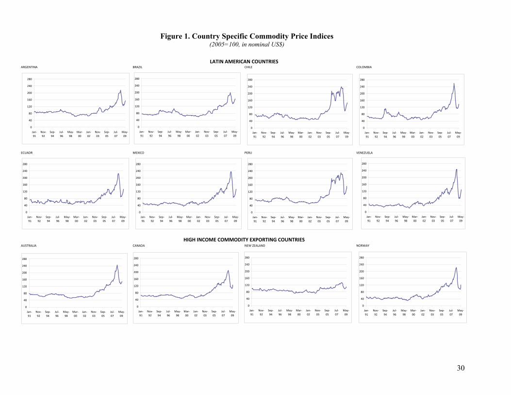
However, the recent plunge in commodity prices and global trade since late 2008 has

affected net commodity-producing countries (Figure 1). As a result, government finances

have come under pressure in many countries in the region.

Episodes of booms and busts in commodity prices generate volatility in the fiscal

revenues of emerging commodity-exporting countries (Figure 2). Some governments,

assuming that a boom in prices may be permanent, increase expenditures more than

proportionally. Once the government expenditures rise (and when the effects of the boom

have faded out) it is very difficult to lower them, such as described in Boccara (1994).

Since this kind of behavior seems to be quite pervasive in the region, it is important to

explore its causes and consequences.

Recent literature has typically focused on documenting the reaction of fiscal positions to

the output cycle and only indirectly linking commodity price fluctuations with fiscal

outcomes, looking at the impact of commodity prices only through their effect on GDP.

3

For instance, Gavin and Perotti (1997) identify the procyclicality of fiscal policy in LA

particularly in periods of low growth. Talvi and Végh (2005) generalized this claim to all

developing countries. Kaminsky, Reinhart and Végh (2004) not only find evidence of

procyclicality of fiscal policy, capital flows and monetary policy in developing countries,

particularly in middle-high income countries, but also analyze which indicators are

appropriate to measure the procyclical behavior. Ilzetzki and Végh (2008) discover

evidence of the procyclicality of fiscal policy in developing countries and that it is

expansionary. The explanation for this procyclical behavior has been attributed to

international credit constraints and political distortions in the literature,2 but the literature

has not focused on the direct impact of external shocks on fiscal positions.

To account for the cyclicality of fiscal policy, several measures have been used. Ilzetzki

and Végh (2008) use government consumption (from the national accounts); Kaminsky

et. al. (2004) utilize government spending, while Gavin and Perotti (1997) and Alesina

and Tabellini (2005) exploit the fiscal deficit. The use of government consumption is not

very convenient from a comprehensive discretionary perspective, because it does not take

into consideration government investment (capital expenditures), key in emerging

exporting economies especially during commodity price booms. With respect to the use

of fiscal balance, the problem is that it is difficult to extract the effect of an external

shock, because when a positive shock hits, government revenues increase right away due

to the increase in export taxes, particularly in commodity exporting countries. Therefore,

using fiscal deficit as the variable of interest, one could erroneously say that there is no

2 On the international credit constraint literature see Gavin and Perotti (1997), Riascos and Végh (2003) , and Caballero and Krishnamurthy (2004). With respect to the literature on political distortions, see Tornell and Lane (1999) , Talvi and Végh (2005), Alesina and Tabellini (2005) and Ilzetzki (2008).

4

impact of external shocks on fiscal positions, while what is really happening is that there

is an impact in both revenues (automatically through export taxes) and expenditures

(discretionary).

Research has also referred to the impact of commodity price shocks on economic

aggregates. Hirschman (1977) cites the mid-nineteenth-century Peruvian guano boom,

the benefits of which were misspent in railway investments; Collier and Gunning (1994)

attribute the Egyptian loss of the Suez Canal to the unsustainable Egyptian public-

expenditure programs following the cotton-price boom during the U.S. Civil War. Deaton

and Miller (1995) assess the impact of commodity price shocks on Sub-Saharan Africa

and discuss whether poor macroeconomic results should be attributed to the inherent

difficulty of predicting commodity-price fluctuations or, rather, to flawed internal

political and fiscal arrangements. Raddatz (2007) finds that, among external shocks,

commodity prices are the most important source of fluctuation on low income countries’

per-capita GDP and that, in response to shocks, the government expenditure and the

current account tend to move in tandem with total GDP. However, this literature has not

analyzed the dynamic responses of fiscal positions to the commodity price shocks.

To look at the impact of commodity prices on economic aggregates, some studies have

constructed country specific commodity price indices. For example, Deaton and Miller

(1995) assembled a measure of export prices for 32 countries. For each one of the

countries, they calculated the total value of exports of 21 commodities in 1975 and

weight them by dividing the value of each commodity’s exports in 1975 by this total. The

weights are then held constant for the rest of the exercise and are applied to the world

5

prices of the same commodities. Collier and Goderis (2007) constructed a commodity

export price index composed by agricultural and non-agricultural commodities at a yearly

frequency with fixed commodity export weights; to allow the effect of commodity export

price to be larger for countries with larger exports, they weight the index by the share of

commodity exports in GDP. The use of fixed weights in these indices does not allow

accounting for the impact of changes in the trade shares.

Taking into account the literature above, as well as the unprecedented magnitude of the

last boom and bust behavior of commodity prices, an analysis that focuses on

understanding the direct impact of commodity prices on fiscal positions is needed. This

paper makes three contributions to the existing literature: (i) it uses a novel quarterly

dataset that includes a unique country specific commodity price index, that allows to look

at changes in commodity prices and changes in the commodity export shares (ii) it

exploits a comprehensive measure of public expenditure and (iii) it analyses the dynamic

effects of commodity prices on revenues, expenditures and GDP using VAR

methodology that relies on Cholesky decomposition of matrices for the identification

strategy. The novelty of this approach is that I will estimate the impact of commodity

price shocks on fiscal variables using a unique dataset, while the existing empirical

studies focus typically on the procyclicality of fiscal variables (government expenditure,

primary surplus) with respect to GDP and on the impact of fiscal variables on GDP

(fiscal multiplier).

6

The results of the estimations indicate that LA countries fiscal positions generally react

strongly to positive shocks to commodity prices, however, they highlight that there exists

a spectrum of responses. Within this spectrum Chile behaves like an outlier in the LA

region with dynamic fiscal responses to commodity prices fluctuations very similar to the

high-income commodity exporting countries, such as Australia, Canada, New Zealand

and Norway. At the other end of the spectrum is Venezuela where expenditures rise even

more than proportionally than revenues when faced with a commodity price shock.

The remainder of this paper is organized as follows: The next section includes the

description of a suggested methodology to study the impact of commodity prices on

fiscal positions and describes the data used. The third section describes and analyses the

main results. The last section concludes and suggests possible avenues for future

research.

II. COMMODITY PRICES AND THEIR DYNAMIC IMPACT ON FISCAL

POSITIONS: A SUGGESTED METHODOLOGY

1. Vector Autoregression (VAR) approach

To estimate the effects of commodity price shocks on fiscal positions, I will estimate a

VAR model using as identification strategy the Cholesky decomposition of matrices. A

desirable property of VARs (given the purpose of this exercise) is that they focus on the

impact of shocks. First the relevant shocks are identified, and the response of the system

7

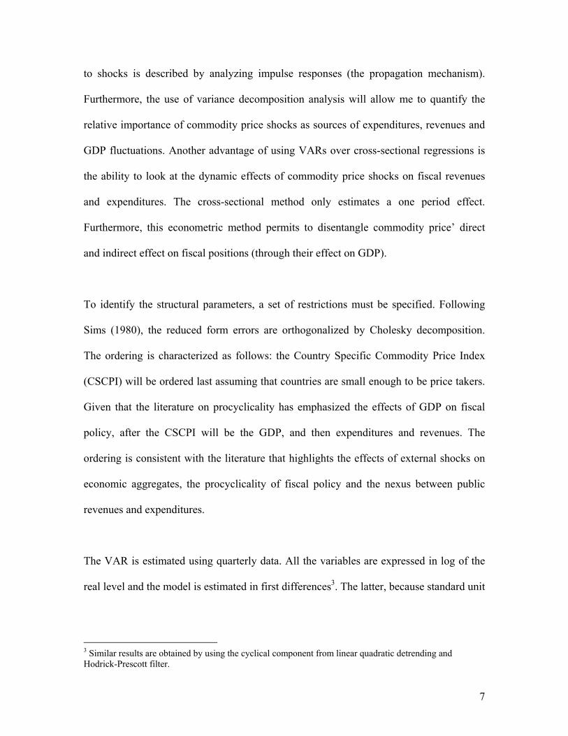
to shocks is described by analyzing impulse responses (the propagation mechanism).

Furthermore, the use of variance decomposition analysis will allow me to quantify the

relative importance of commodity price shocks as sources of expenditures, revenues and

GDP fluctuations. Another advantage of using VARs over cross-sectional regressions is

the ability to look at the dynamic effects of commodity price shocks on fiscal revenues

and expenditures. The cross-sectional method only estimates a one period effect.

Furthermore, this econometric method permits to disentangle commodity price’ direct

and indirect effect on fiscal positions (through their effect on GDP).

To identify the structural parameters, a set of restrictions must be specified. Following

Sims (1980), the reduced form errors are orthogonalized by Cholesky decomposition.

The ordering is characterized as follows: the Country Specific Commodity Price Index

(CSCPI) will be ordered last assuming that countries are small enough to be price takers.

Given that the literature on procyclicality has emphasized the effects of GDP on fiscal

policy, after the CSCPI will be the GDP, and then expenditures and revenues. The

ordering is consistent with the literature that highlights the effects of external shocks on

economic aggregates, the procyclicality of fiscal policy and the nexus between public

revenues and expenditures.

The VAR is estimated using quarterly data. All the variables are expressed in log of the

real level and the model is estimated in first differences3. The latter, because standard unit

3 Similar results are obtained by using the cyclical component from linear quadratic detrending and Hodrick-Prescott filter.

8

root tests show that the variables are stationary in first differences. The number of

included lags (1 to 6) was determined based on the Hannan-Quinn information criterion.

2. Data

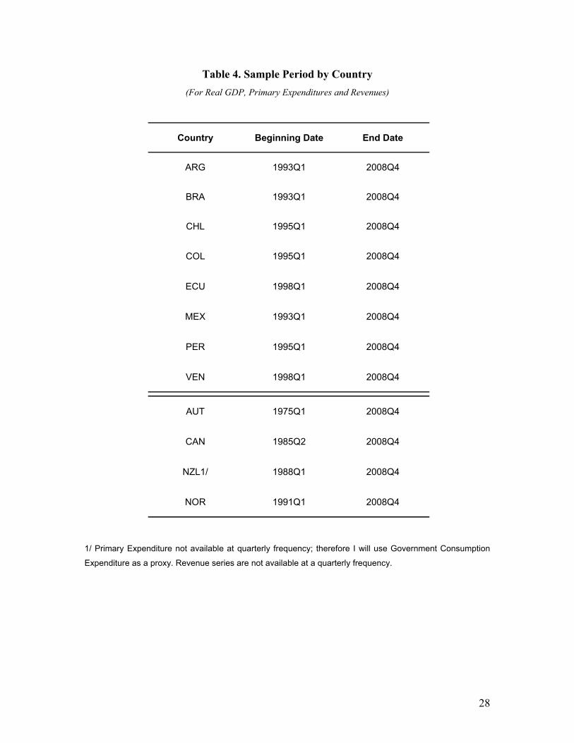
In order to study the effects of commodity price fluctuations on fiscal positions, I will use

a novel database for 12 commodity exporting countries, covering a period that spans as

early as the first quarter of 1975 to as late as the last quarter of 2008, but differs from

country to country. This dataset will use unique Country Specific Commodity Price

Indices (CSCPI) that combine international prices of 55 commodities (IMF, monthly

commodity price indices) and commodity export shares by country (from the Standard

International Trade Classification, SITC, found in the World Integrated Trade Solutions,

WITS). The CSCPI will allow me to look not only at changes of commodity prices, but

also at the composition of commodity exports.

For this exercise a sample of 12 countries was selected: the Latin American largest

commodity exporting countries and four high income commodity exporting countries.

The Latin American sample includes Argentina, Brazil, Chile, Colombia, Ecuador,

Mexico, Peru and Venezuela. These countries account for more than 92 percent of LA’s

GDP. Furthermore, their commodity exports represent, on average, more than 55 percent

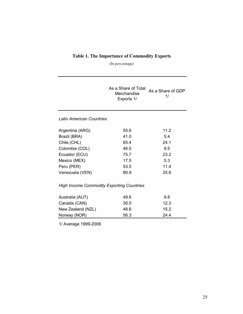
of total exports of goods, which also represent a large share of GDP (Table 1). In order to

compare the performance of LA with other economies with similar features, four high

9

income commodity exporting countries were added to the sample: Australia, Canada,

New Zealand and Norway.

The variables of interest are government primary expenditures, revenues, real GDP and

the Country Specific Commodity Price Indices (CSCPI). Government revenues and

primary expenditure for the Non Financial Public Sector (NFPS) were used because they

give a broader aggregation level. When these series were not available at this level,

Central Government variables were utilized. See the Appendix for a more detailed

description of the data used and its sources.

The CSCPI is based on both the IMF monthly commodity price indices and the trade

information from the Standard International Trade Classification (SITC) found in the

World Integrated Trade Solution (WITS)4.

The procedure to create the CSCPI requires linking commodity prices from the IMF with

the commodity’s trade value from the WITS. When the commodity is found in both

datasets, this relationship is direct. Nonetheless, the link could be indirect since the

information from the IMF has only 55 commodities while the WITS has 196. Linking

these data requires some assumptions: either more than one commodity from the WITS

could be classified in the same commodity group of the IMF or some of the commodities

in the WITS could not be linked to a commodity price in the IMF dataset. It is important

to note that the frequency of the information is also different. The IMF database is

monthly while the WITS is annual. In order to take advantage of the high frequency for

4 It is important to clarify that the SITC has 3 revisions. In this case, I use the third one because it includes more commodities than the previous data. Data could be disaggregated into 3 or 4 digits.

10

the prices database, I assume the weights for each commodity are the same for each year

throughout the sample period. The weights reflect, on average, 80 to 90 percent of the

total commodity exports.

All variables are expressed in real terms. Whenever the original series were not in real

terms, the nominal variables were deflated by the Consumer Price Index. All series are in

logs and, when not reported in seasonally-adjusted terms (except for the CSCPI), they are

adjusted using the X-12 quarterly seasonal adjustment method5.

As the presented data follows a nonstationary process, tests for unit roots were performed

and the unit roots hypothesis was not rejected. Furthermore, Johansen cointegration

procedure was performed for all the variables in the system and the results shows that

there is no cointegration vector under the model considered. In consequence, these series

were adjusted to be stationary in order to be included in the VAR estimation. The results

are robust to other specifications, such as the cyclical component of the series obtained

by using the Hodrick-Prescott filter.

III. RESULTS

1. The dynamic responses of fiscal variables to commodity price shocks

1.1 The size of the shock

5 This method ( published by the U. S. Department of Commerce, U. S. Census Bureau) modifies the X-11 variant of Census Method II by J. Shiskin A.H. Young and J.C. Musgrave of February, 1967.

11

When looking at the country specific commodity prices, one can observe a significant

acceleration in commodity prices starting at the end of 2003, tendency that lasted till

september of 2008 where there was a bust. Nevertheless prices never returned to their

pre-2003 levels.

When computing the price shocks in the VARs, on average, the size of the one standard

deviation shock in LAC countries is of around 13 percent, being Venezuela the largest

with 16.4 percent and Brazil the smallest with 7.8 percent (Figure 4). With respect to

high-income commodity exporters, the largest on impact response is that of Norway, that

reaches almost 10 percent.

Another interesting feature of these indices –that affect the size of the shocks- is their

composition. While Argentina mainly focus on soy and beef, other LA countries and

high-income commodity exporters heavily rely on metals, minerals and oil. The

exception to the high-income group is New Zealand (Table 2).

1.2 Impulse response function analysis

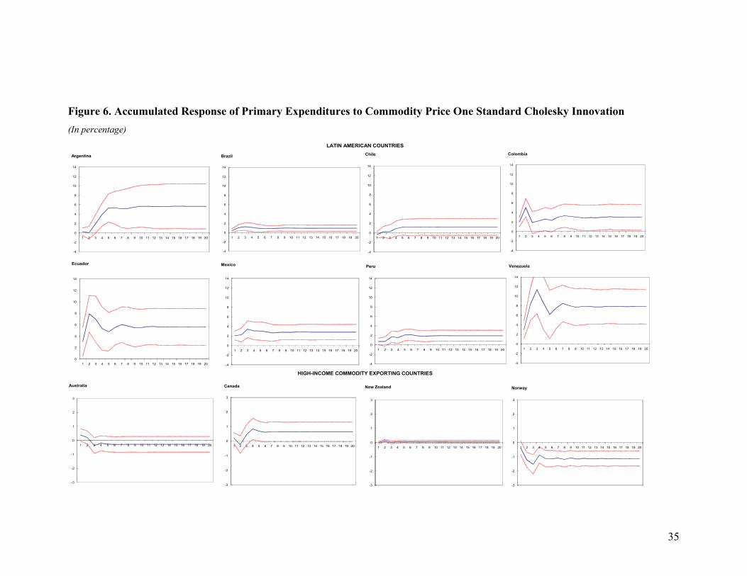
The estimated accumulated impulse response functions are shown in Figures 5, 6, 7 and

8. Dotted lines reflect one-standard deviation bands. The solid line represents the

respective accumulated response to Cholesky one standard deviation commodity price

shocks.

12

For both LA and high-income countries, positive commodity price shocks have the

expected positive impact on real revenues and GDP. A one-standard deviation shock to

commodity prices in a quarter leads to a rise in government real revenues that range from

around 2 percent in Brazil and Canada, to 10 percent in Venezuela and around 14 percent

in Ecuador. With respect to GDP, the same shock generates a response that varies from

around 1 percent in Australia, to 2.5 percent and 3 percent in Argentina and Norway

respectively. In most cases, the peak response of revenues and GDP occur two quarters

after the shock (Table 5).

Compared with the behavior of revenues and GDP, however, the response primary

expenditures to commodity prices is substantially more heterogeneous across Latin

American countries. A positive innovation to the commodity price leads to responses that

range from 0 percent in the case of Chile, to an increase of almost 12 percent in

Venezuela.6 The median response is around 4 percent, and the second largest response

(from Colombia) is less than 8 percent, indicating that Venezuela behaves like an outlier

in the regional context (Figure 6).

In the case of high-income commodity exporters, a standard deviation in the commodity

price shock in a quarter, leads to no reaction of primary expenditures in Australia and

New Zealand. In Canada and Norway, primary expenditures actually decrease on impact

6 The results for Chile are consistent with findings by other authors, like Kaminsky et. al. (2004) and

Calderon and Schmidt-Hebbel (2003).

13

(with reactions of -0.2 percent and -1.5 percent, respectively), suggesting a counter-

cyclical fiscal policy.

Taken together, the results show that while both LA and high-income countries revenues

and GDP react positively to commodity price shocks, a completely different set of results

is found when looking at the impact in primary expenditures. Within LA there is a wide

dispersion in country’s responses, with Venezuela and Chile at opposing ends of the

spectrum of responses. The response of fiscal indicators in Chile, in particular, resemble

those seen in high-income commodity exporting countries.

1.3. Variance decomposition analysis

To quantify the contribution of commodity price shocks to fluctuations in government

expenditures, I estimate variance decomposition of forecast errors. Interestingly, the

results from this analysis (Table 3 and Figure 3) show that commodity price fluctuations

play a dominant role in Venezuela (the highest), accounting for almost 17 percent of

government spending fluctuations at a 10 quarters horizon. In Chile, on the hand,

commodity price fluctuations hardly explain expenditure fluctuations at all, accounting

for less than 4 percent in the same time horizon, almost four times less than in Venezuela.

All other LA countries lie in between Chile and Venezuela, with an average contribution

(excluding Venezuela and Chile) of 9.5 percent at a 10 quarters horizon.

14

Results for high-income commodity exporting countries indicate that, on average,

commodity price fluctuations explain a smaller fraction of government expenditures

fluctuations than in LA countries, averaging 3.8 percent at a 10 quarters horizon.

2. Looking at fiscal rules

A possible explanation to the different behavior in expenditures is likely related to the

heterogeneous institutional frameworks that govern fiscal policy decisions. For instance,

Corbacho and Schwartz (2007) suggest that for Argentina, Colombia and Peru fiscal

performance continued to worsen after the fiscal responsibility laws were implemented

(Argentina in 1999, Colombia in 2003 and Peru in 1999). These laws “…fail to substitute

for political commitment and society’s support for needed fiscal consolidation.

Numerical targets where successively breached, undermining credibility in the fiscal

framework established in the law”. With respect to Chile, Kaminsky et. al. (2004) and

Calderon and Schmidt-Hebbel (2003) find evidence that supports the hypothesis that a

country with better fundamentals, stronger institutions and more stable policy rules,

would be able to pursue counter-cyclical policies. The adoption of fiscal rules specifically

designed to encourage public saving in good times may have helped in this effort in the

case of Chile.

When looking at high-income commodity exporting countries, either formal or informal

fiscal rules seem to be accompanied by strong institutions, political commitment and high

standards of transparency, which allow fiscal rules to work. According to Bhattacharyya

15

and Williamson (2009) commodity price shocks that matched most of the primary-

product exporting countries, never caused the same volatility in Australia (either in

aggregates, or in sectoral and regional performance). The explanation is that (i) revenues

come from fairly diverse sources so that commodity price volatility do not produce as

great revenue volatility; (ii) diversification offsets the impact of commodity price shocks;

a big and growing industrial sector before the seventies and a big and growing service

sector after that period seems to make the difference.

In the case of Canada, its strong fiscal record in recent years rests on a proven budgetary

framework, including a well-establish forecasting process. Canadian public finances are

highly transparent, and the prudent fiscal policies of recent governments have had public

support. Unlike in many other countries, fiscal policy is not constrained by budget rules

imposed under the constitution or the law. Between 1998 and 2006, Canada followed a de

facto fiscal rule of “budget balance”. The conservative government that took power in

2006 abandoned this rule in favor of targeting a moderate surplus of 0.25 percent of

GDP.

For New Zealand, by early 1990’s, policy advice was oriented toward fiscal consolidation

and a medium-term focus. Changes to the institutional framework were made, following

the introduction of the Fiscal Responsibility Act (1994). The Act is based on “principles"

of responsible fiscal management, including strong disclosure and reporting

requirements, but does not set fixed numerical targets.

16

In order to manage Norway’s oil wealth a Government Petroleum Fund was establish in

1990. It receives most of the petroleum revenue and invests it in financial assets abroad.

The key fiscal rule sets non-oil structural budget deficit of the central government to be 4

percent (allowing for temporary deviations over the business cycle). The fund was

created to preserve assets for future generations and avoid potential crowding out effects

(Dutch disease) that the rapid spending of oil wealth might carry.

IV. CONCLUSION

In light of the recent boom and bust in commodity prices, concerns have been raised

about the impact of commodity prices on Latin American countries’ fiscal positions.

Given that the size of the last shock has been unprecedentedly large it is important to

study its effect on commodity exporting countries’ fiscal positions.

This paper estimates the dynamic effects of commodity price shocks in a group of LA

commodity exporting countries and compares VAR impulse responses functions with

those of high-income commodity exporting countries. This methodology exploits the use

of a unique quarterly dataset that includes a novel country specific commodity price

index. The results of the estimations show that the impact in revenues is not that different

among the two groups of countries. In contrast, there is a spectrum of primary

expenditures responses within LA countries, being Chile and Venezuela the extremes of

the distribution. Furthermore, Chile behaves similar to high-income countries.

17

A potential explanation to this behavior could be the efficient application of fiscal rules,

accompanied by strong institutions, political commitment and high standards of

transparency. This hypothesis has been recognized by other literature, where there seems

to be agreement about the influence of fiscal institutions on fiscal performance (Corbacho

and Schwartz (2007)). A possible next step for this research would be to look for

structural breaks in countries that during the last decade adopted fiscal rules, to be able to

detect changes in fiscal behavior and establish if there is a clear empirical link with such

rules.

18

V. REFERENCES

Alesina, A. and G. Tabellini; “Why is Fiscal Policy Often Procyclical?” NBER Working

Paper No. 11600; 2005.

Bhattacharyya S. and J. Williamson; “Commodity Price Shocks and the Australian

Economy Since Federation”; NBER Working Paper No. 14694; 2009.

Blanchard O. and R. Perotti; “An Empirical Characterization of the Dynamics Effects of

Changes in Government Spending and Taxes on Output”; NBER, 1999.

Boccara B. ;”Why Fiscal Spending Persists When a Boom in Primary Commodities

Ends”; The World Bank; 1994.

Caballero, R. J., and A. Krishnamurthy; “Fiscal policy and financial depth”; NBER

Working Paper No. 10532. 2004.

Calderon C. and K. Schmidt-Hebbel; “Macroeconomic Policies and Performance in Latin

America”; Journal of International Money and Finance; Vol. 22; pp. 895-923; 2003.

Calderon C. and P. Fajnzylber; “How Much Room Does Latin America And The

Caribbean Have For Implementing Counter-Cyclical Fiscal Policies?”; April, 2009.

19

Collier P. and B. Goderis; “Commodity Prices, Growth and the Natural Resource Curse:

Reconciling a Conundrum”; University of Oxfords; 2007.

Collier P. and J. Gunning; “Trade Shocks: Consequences and Policy Responses in

Developing Countries”; San Francisco; International Center for Economic Growth; 1994.

Corbacho A. and Schwartz G; “Fiscal Responsibility Laws” in Kumar, M. S. and Ter-

Minassian T.(eds);”Promoting Fiscal Discipline”; International Monetary Fund; 2007.

Deaton A. and R. Miller; “International Commodity Prices, Macroeconomic

Performance, and Politics in Sub-Saharan Africa”; Princeton Studies in International

Finance 79. 1995.

Gavin M. and R. Perotti; ”Fiscal Policy in Latin America”: NBER Macroeconomics

Annual. 1997.

Hirschman A.; “A Generalized Linkage Approach to Development, with Special

Reference to Staples”; Economic Development and Cultural Change; 25; 1977.

Hodrick R. and Prescott E.; "Postwar U.S. Business Cycles: An Empirical Investigation";

Journal of Money, Credit, and Banking; 1997.

20

Ilzetzki, E.; “Rent-seeking distortions and fiscal pro-cyclicality.” University of Maryland,

manuscript, December 2008.

Ilzetzki, E., and C.A. Végh: “ Pro-cyclical fiscal policy in developing countries: Truth or

fiction?”; NBER Working Paper 14191, July 2008.

International Monetary Fund; Western Hemisphere: Regional Economic Outlook;

“Saving for a Rainy Day? Sensitivity of LAC Fiscal Positions to Commodity Prices”; Di

Bella G., H. Kamil and L. Medina; 2009.

International Monetary Fund: “Norway: Selected Issues”; Rossi M., Jafarov E. and Leigh

D.; May 2007.

International Monetary Fund: “Western Hemisphere: Regional Economic Outlook”; April

2008.

Kaminsky, G.L., C.M. Reinhart, and C.A. Végh; “When it rains, it pours: Procyclical

capital flows and macroeconomic policies.” In: Gertler, M., and K. Rogoff, eds., NBER

Macroeconomics Annual 2004. Cambridge, MA: The MIT Press 2005.

Perron P.; “The Great Crash, the Oil Price Shock, and the Unit Root Hypothesis”;

Econometrica 57 Nov 1989.

21

Perotti R.; “Fiscal Policy in Developing Countries: A Framework and Some Questions”;

The World Bank: 2007.

Raddatz C.; “Are external shocks responsible for the instability of output in low-income

countries?”; Journal of Development Economics; Elsevier, vol. 84(1), pages 155-187;

September 2007.

Riascos A. and C. A. Végh; "Procyclical Government Spending in Developing Countries:

The Role of Capital Market Imperfections."; mimeo, UCLA and Banco Republica,

Colombia; 2003.

Sims, C.; “Macroeconomics and Reality”; Econometrica; 48(1); 1980.

Talvi E. and C. A. Végh ;"Tax Base Variability and Pro-cyclical Fiscal Policy in

Developing Countries"; Journal of Development Economics 78 (1): 156-190. 2005.

Tornell A. and P. Lane; “Are windfalls a curse? A nonrepresentative agent model of the

current account"; Journal of International Economics 44, pp. 83-112; 1998.

Tornell A. and P. Lane; ”The Voracity Effect”; American Economic Review, Vol. 89;

1999, pp. 22-46.

22

VI. APPENDIX

1. Data

The Data presented in this paper goes as far as the first quarter of 1975. For more

information about the length of the time series for each country please see Table 4.

Next is a description of the series and data sources.

Country Specific Commodity Price Indices

Author’s estimations based on the IMF monthly commodity price indices and the trade

data from the Standard International Trade Classification (SITC) found in the World

Integrated Trade Solution (WITS).

Real GDP

Data was obtained by Haver Analytics using primary data from each country’s

authorities. When real data was not available, nominal data was deflated by each

country’s CPI.

CPI

The series on CPI were obtained by Haver Analytics using primary data from each

country’s authorities.

Revenues and Primary Expenditures

23

Revenues encompass total revenues and the aggregation level depends on each country’s

data availability. In the case of primary expenditures, the variable cover total

expenditures (i.e. current expenditures plus capital expenditures) minus interest

payments; aggregation level depending also on country’s definitions and data

availability.

For Argentina, author’s estimations from the Non-Financial Public Sector data, published

by the Finance Ministry. In the case of Australia, Central Government aggregation data

from the Reserve Bank of Australia. For Brazil, the series were used at a Central

Government level (including Federal Government, Central Bank and Social Security

Administration) from the Central Bank database. Data for Canada was obtained by Haver

Analytics using primary data from Canada’s Department of Finance at a Federal

Government aggregation level. The series for Chile were obtain from the Finance

Ministry at a Central Government level. For Colombia, data for the Non-Financial Public

Sector was gathered from the Finance Ministry’s CONFIS. In the case of Ecuador, the

data was obtained at a Non-Financial Public Sector level from Ecuador’s Central Bank.

For Mexico, Central Government data was acquired from the Finance and Public Credit

Department. New Zealand data on government revenues and expenditures were not

available at a quarterly basis, therefore, data on government consumption were used

(from the country’s national accounts). The series for Norway were gathered at a Central

Government level (including National Insurance Scheme) from Statistics Norway. For

Peru, data was obtained at a Central Government level from Peru’s Central Bank. In the

24

case of Venezuela, data was gathered at a Central Government level from Venezuela’s

Central Bank.

25

Table 1. The Importance of Commodity Exports

(In percentage)

As a Share of Total Merchandise

Exports 1/

As a Share of GDP 1/

Latin American Countries

Argentina (ARG) 55.6 11.2

Brazil (BRA) 41.0 5.4

Chile (CHL) 65.4 24.1

Colombia (COL) 46.0 9.5

Ecuador (ECU) 75.7 23.2

Mexico (MEX) 17.5 5.3

Peru (PER) 53.5 11.4

Venezuela (VEN) 80.9 25.6

High Income Commodity Exporting Countries

Australia (AUT) 49.6 9.8

Canada (CAN) 30.0 12.3

New Zealand (NZL) 48.6 15.2

Norway (NOR) 56.3 24.4

1/ Average 1999-2006

26

Table 2. Country Specific Commodity Price Indices Composition 1/

(2005, in percentage)

ARG BRA CHL COL ECU MEX PER VEN AUS CAN NZL NOR

Aluminum 1.9 4.9 0.1 0.6 0.3 0.3 0.0 2.1 5.6 6.1 5.4 5.0

Banana 3.0 1.6 6.0 5.2 14.1 3.7 1.6 0.0 0.7 0.1 6.4 0.0

Barley 0.2 0.0 0.0 0.0 0.0 0.0 0.0 0.0 0.9 0.3 0.0 0.0

Beef 6.9 10.6 1.6 2.0 0.0 2.2 0.0 0.0 9.3 4.0 27.8 0.0

Butter 0.1 0.0 0.0 0.0 0.0 0.0 0.0 0.0 0.3 0.0 5.3 0.0

Cheese 0.6 0.1 0.2 0.1 0.0 0.0 0.0 0.0 1.0 0.1 6.0 0.1

Chicken 0.0 0.0 0.0 0.0 0.0 0.0 0.0 0.0 0.0 0.0 0.0 0.0

Coal 0.0 0.0 0.0 25.0 0.0 0.0 0.0 0.7 26.9 2.8 0.0 0.0

Cocoa 0.4 0.9 0.1 0.5 2.1 0.3 0.4 0.0 0.2 0.7 0.6 0.0

Coconut oil 0.0 0.0 0.0 0.0 0.0 0.0 0.0 0.0 0.0 0.0 0.0 0.0

Coffee 0.0 6.9 0.0 15.7 1.1 0.8 3.2 0.0 0.1 0.2 0.0 0.0

Copper 3.4 1.7 64.4 0.3 0.0 2.5 37.1 0.0 5.3 2.8 0.2 0.3

Cotton 0.2 1.3 0.0 0.2 0.1 1.0 0.5 0.0 1.3 0.2 0.0 0.0

Cotton seed oil 0.0 0.1 0.0 0.0 0.0 0.0 0.0 0.0 0.0 0.0 0.0 0.0

Crude oil 11.6 9.9 0.0 38.8 66.8 74.7 2.0 96.7 7.8 23.3 2.2 61.5

Eggs 0.0 0.1 0.0 0.0 0.0 0.0 0.1 0.0 0.0 0.0 0.0 0.0

Fish 3.5 1.0 9.1 1.7 12.1 1.6 3.4 0.1 1.5 3.3 6.9 6.3

Groundnut oil 0.3 0.0 0.0 0.0 0.0 0.0 0.0 0.0 0.0 0.0 0.0 0.0

Groundnuts 0.2 0.1 0.0 0.0 0.0 0.0 0.0 0.0 0.0 0.0 0.0 0.0

Hides 0.0 0.0 0.0 0.1 0.0 0.4 0.0 0.0 0.8 0.5 1.2 0.1

Iron 0.0 0.0 0.0 0.0 0.0 0.0 0.0 0.0 0.4 0.8 0.5 0.1

Iron ore 0.1 17.1 1.1 0.1 0.0 0.3 2.3 0.0 13.5 1.3 0.1 0.1

Jute 0.0 0.0 0.0 0.0 0.0 0.0 0.0 0.0 0.0 0.0 0.0 0.0

Lead 0.1 0.0 0.0 0.0 0.0 0.1 4.6 0.0 1.4 0.2 0.1 0.0

Linseed oil 0.0 0.0 0.0 0.0 0.0 0.0 0.0 0.0 0.0 0.0 0.0 0.0

Maize 6.2 0.3 0.3 0.0 0.1 0.0 0.1 0.0 0.1 0.3 0.0 0.0

Manganese ores 0.0 0.3 0.0 0.0 0.0 0.0 0.0 0.0 0.6 0.0 0.0 0.0

Milk 1.9 0.2 0.2 0.4 0.0 0.2 0.4 0.0 1.6 0.1 17.7 0.0

Nat gas 5.6 0.1 0.2 0.2 0.0 0.2 0.9 0.0 5.6 29.6 0.0 23.7

Nickel 0.0 0.6 0.0 0.0 0.0 0.0 0.0 0.0 1.6 3.2 0.0 1.6

Olive oil 0.2 0.0 0.0 0.0 0.0 0.0 0.0 0.0 0.0 0.0 0.0 0.0

Palm oil 0.0 0.0 0.0 0.9 0.6 0.0 0.0 0.0 0.0 0.0 0.0 0.0

Pepper 0.0 0.2 0.1 0.1 0.0 0.1 1.0 0.0 0.0 0.0 0.0 0.0

Platinum 0.0 0.0 0.0 0.1 0.0 0.0 0.0 0.0 0.0 0.0 0.0 0.2

Poultry 0.0 0.0 0.0 0.0 0.0 0.0 0.0 0.0 0.0 0.1 0.1 0.0

Rice 0.4 0.1 0.0 0.0 0.2 0.0 0.0 0.0 0.1 0.0 0.0 0.0

Rubber 0.2 0.7 0.0 0.0 0.0 0.6 0.0 0.0 0.0 0.3 0.0 0.0

Silver 0.1 0.2 0.7 0.4 0.0 1.9 3.6 0.0 0.2 0.5 0.0 0.0

Soft Log 0.6 3.1 3.7 0.1 0.5 0.3 1.3 0.0 0.2 9.0 7.2 0.2

Soy oil 13.4 3.0 0.0 0.1 0.0 0.2 0.0 0.0 0.1 0.5 0.0 0.0

Soybean meal 17.7 7.0 0.0 0.1 0.3 0.2 12.4 0.0 0.9 0.6 1.0 0.2

Soybeans 10.2 12.5 0.0 0.0 0.0 0.0 0.0 0.0 0.0 0.3 0.0 0.0

Sugar 1.9 10.2 0.6 5.3 1.2 2.9 0.4 0.0 0.7 1.8 4.6 0.1

Swine 0.0 0.2 0.0 0.0 0.0 0.1 0.0 0.0 0.0 0.7 0.0 0.0

Tea 0.3 0.1 0.0 0.0 0.0 0.0 0.0 0.0 0.0 0.0 0.0 0.0

Tin 0.0 0.2 11.1 1.0 0.1 2.9 14.3 0.1 0.9 1.3 0.5 0.1

Tobbaco 0.9 3.9 0.0 0.1 0.3 0.1 0.1 0.0 0.0 0.1 0.0 0.0

Uranium 0.0 0.0 0.0 0.0 0.0 0.0 0.0 0.0 0.7 0.0 0.0 0.0

Wheat 7.0 0.3 0.3 0.8 0.0 1.5 0.5 0.1 4.4 3.9 2.4 0.0

Wool 0.7 0.0 0.1 0.0 0.0 0.0 0.3 0.0 2.8 0.0 3.8 0.0

Zinc 0.1 0.2 0.1 0.0 0.0 1.1 9.3 0.0 2.2 0.8 0.0 0.3

1/ Highlighted commodities represent more than 50 percent of each index composition.

Table 3. Commodity Price Shocks as a Source of Primary Expenditure Fluctuations

(Contribution of commodity price shocks to the variance of primary expenditure growth)

Quarters after the shock

VEN COL ARG ECU MEX BRA PER CHL

1 5.73 6.84 0.02 4.19 10.57 2.61 1.56 0.60

2 14.52 11.13 0.60 9.69 6.74 7.38 1.49 1.96

4 16.83 15.57 12.97 9.47 8.22 7.42 3.40 3.64

8 16.61 14.32 12.47 9.69 8.23 7.84 4.12 3.92

10 16.59 14.26 12.90 9.72 8.23 7.85 4.12 3.92

Quarters after the shock

CAN NZL NOR AUT

1 0.38 0.00 0.86 0.60

2 1.79 3.26 2.72 0.54

4 5.54 5.26 3.47 1.49

8 5.70 5.39 2.92 1.50

10 5.71 5.39 2.91 1.50

28

Table 4. Sample Period by Country

(For Real GDP, Primary Expenditures and Revenues)

Country Beginning Date End Date

ARG 1993Q1 2008Q4

BRA 1993Q1 2008Q4

CHL 1995Q1 2008Q4

COL 1995Q1 2008Q4

ECU 1998Q1 2008Q4

MEX 1993Q1 2008Q4

PER 1995Q1 2008Q4

VEN 1998Q1 2008Q4

AUT 1975Q1 2008Q4

CAN 1985Q2 2008Q4

NZL1/ 1988Q1 2008Q4

NOR 1991Q1 2008Q4

1/ Primary Expenditure not available at quarterly frequency; therefore I will use Government Consumption

Expenditure as a proxy. Revenue series are not available at a quarterly frequency.

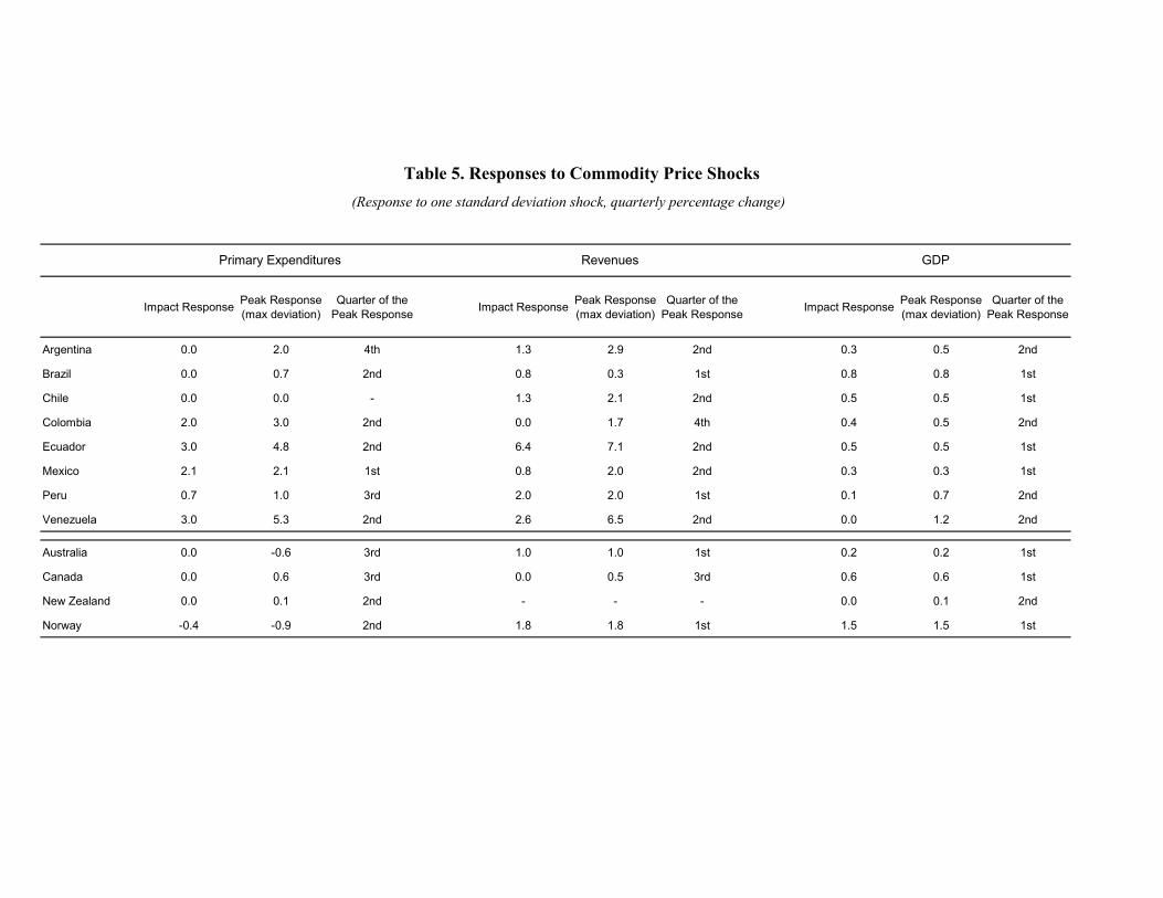
Table 5. Responses to Commodity Price Shocks

(Response to one standard deviation shock, quarterly percentage change)

Impact ResponsePeak Response (max deviation)

Quarter of the Peak Response

Impact ResponsePeak Response (max deviation)

Quarter of the Peak Response

Impact ResponsePeak Response (max deviation)

Quarter of the Peak Response

Argentina 0.0 2.0 4th 1.3 2.9 2nd 0.3 0.5 2nd

Brazil 0.0 0.7 2nd 0.8 0.3 1st 0.8 0.8 1st

Chile 0.0 0.0 - 1.3 2.1 2nd 0.5 0.5 1st

Colombia 2.0 3.0 2nd 0.0 1.7 4th 0.4 0.5 2nd

Ecuador 3.0 4.8 2nd 6.4 7.1 2nd 0.5 0.5 1st

Mexico 2.1 2.1 1st 0.8 2.0 2nd 0.3 0.3 1st

Peru 0.7 1.0 3rd 2.0 2.0 1st 0.1 0.7 2nd

Venezuela 3.0 5.3 2nd 2.6 6.5 2nd 0.0 1.2 2nd

Australia 0.0 -0.6 3rd 1.0 1.0 1st 0.2 0.2 1st

Canada 0.0 0.6 3rd 0.0 0.5 3rd 0.6 0.6 1st

New Zealand 0.0 0.1 2nd - - - 0.0 0.1 2nd

Norway -0.4 -0.9 2nd 1.8 1.8 1st 1.5 1.5 1st

Primary Expenditures Revenues GDP

30

ARGENTINA BRAZIL CHILE COLOMBIA

ECUADR MEXICO PERU VENEZUELA

AUSTRALIA CANADA NEW ZEALAND NORWAY

LATIN AMERICAN COUNTRIES

HIGH INCOME COMMODITY EXPORTING COUNTRIES

0

40

80

120

160

200

240

280

Jan-91

Nov-92

Sep-94

Jul-96

May-98

Mar-00

Jan-02

Nov-03

Sep-05

Jul-07

May-09

0

40

80

120

160

200

240

280

Jan-91

Nov-92

Sep-94

Jul-96

May-98

Mar-00

Jan-02

Nov-03

Sep-05

Jul-07

May-09

0

40

80

120

160

200

240

280

Jan-91

Nov-92

Sep-94

Jul-96

May-98

Mar-00

Jan-02

Nov-03

Sep-05

Jul-07

May-09

0

40

80

120

160

200

240

280

Jan-91

Nov-92

Sep-94

Jul-96

May-98

Mar-00

Jan-02

Nov-03

Sep-05

Jul-07

May-09

0

40

80

120

160

200

240

280

Jan-91

Nov-92

Sep-94

Jul-96

May-98

Mar-00

Jan-02

Nov-03

Sep-05

Jul-07

May-09

0

40

80

120

160

200

240

280

Jan-91

Nov-92

Sep-94

Jul-96

May-98

Mar-00

Jan-02

Nov-03

Sep-05

Jul-07

May-09

0

40

80

120

160

200

240

280

Jan-91

Nov-92

Sep-94

Jul-96

May-98

Mar-00

Jan-02

Nov-03

Sep-05

Jul-07

May-09

0

40

80

120

160

200

240

280

Jan-91

Nov-92

Sep-94

Jul-96

May-98

Mar-00

Jan-02

Nov-03

Sep-05

Jul-07

May-09

0

40

80

120

160

200

240

280

Jan-91

Nov-92

Sep-94

Jul-96

May-98

Mar-00

Jan-02

Nov-03

Sep-05

Jul-07

May-09

0

40

80

120

160

200

240

280

Jan-91

Nov-92

Sep-94

Jul-96

May-98

Mar-00

Jan-02

Nov-03

Sep-05

Jul-07

May-09

0

40

80

120

160

200

240

280

Jan-91

Nov-92

Sep-94

Jul-96

May-98

Mar-00

Jan-02

Nov-03

Sep-05

Jul-07

May-09

0

40

80

120

160

200

240

280

Jan-91

Nov-92

Sep-94

Jul-96

May-98

Mar-00

Jan-02

Nov-03

Sep-05

Jul-07

May-09

Figure 1. Country Specific Commodity Price Indices (2005=100, in nominal US$)

31

Figure 2. Commodity-Related Fiscal Revenues

(In percentage of GDP)

0

2

4

6

8

10

12

14

16

18

2005 2008 2009p

0

2

4

6

8

10

12

14

16

18

VEN MEX ECU CHL COL ARG PER

32

Figure 3. Contribution of Commodity Price Shocks to the Variance of Primary Expenditure Growth

(In percentage)

0

2

4

6

8

10

12

14

16

18

VEN COL ARG ECU MEX BRA PER CHL CAN NZL NOR AUT

4 quarters after the shock

10 quarters after the shock

33

Figure 4. Response of Commodity Prices to Commodity Price One Standard Cholesky Innovation

(In percentage)

HIGH-INCOME COMMODITY EXPORTING COUNTRIES

LATIN AMERICAN COUNTRIES

-6

-3

0

3

6

9

12

15

18

1 2 3 4 5 6 7 8 9 10 11 12 13 14 15 16 17 18 19 20

Argentina

New Zealand

-6

-3

0

3

6

9

12

15

18

1 2 3 4 5 6 7 8 9 10 11 12 13 14 15 16 17 18 19 20

-6

-3

0

3

6

9

12

15

18

1 2 3 4 5 6 7 8 9 10 11 12 13 14 15 16 17 18 19 20

Brazil

-6

-3

0

3

6

9

12

15

18

1 2 3 4 5 6 7 8 9 10 11 12 13 14 15 16 17 18 19 20

-6

-3

0

3

6

9

12

15

18

1 2 3 4 5 6 7 8 9 10 11 12 13 14 15 16 17 18 19 20

Chile Colombia

-6

-3

0

3

6

9

12

15

18

1 2 3 4 5 6 7 8 9 10 11 12 13 14 15 16 17 18 19 20

-6

-3

0

3

6

9

12

15

18

1 2 3 4 5 6 7 8 9 10 11 12 13 14 15 16 17 18 19 20

Ecuador Mexico

-6

-3

0

3

6

9

12

15

18

1 2 3 4 5 6 7 8 9 10 11 12 13 14 15 16 17 18 19 20

-6

-3

0

3

6

9

12

15

18

1 2 3 4 5 6 7 8 9 10 11 12 13 14 15 16 17 18 19 20

Peru Venezuela

-6

-3

0

3

6

9

12

15

18

1 2 3 4 5 6 7 8 9 10 11 12 13 14 15 16 17 18 19 20

Australia

-6

-3

0

3

6

9

12

15

18

1 2 3 4 5 6 7 8 9 10 11 12 13 14 15 16 17 18 19 20

Canada

-6

-3

0

3

6

9

12

15

18

1 2 3 4 5 6 7 8 9 10 11 12 13 14 15 16 17 18 19 20

Norway

34

Figure 5. Accumulated Response of Commodity Prices to Commodity Price One Standard Cholesky Innovation

(In percentage)

HIGH-INCOME COMMODITY EXPORTING COUNTRIES

LATIN AMERICAN COUNTRIES

0

5

10

15

20

25

30

1 2 3 4 5 6 7 8 9 10 11 12 13 14 15 16 17 18 19 20

Argentina

New Zealand

0

5

10

15

20

25

30

1 2 3 4 5 6 7 8 9 10 11 12 13 14 15 16 17 18 19 20

0

5

10

15

20

25

30

1 2 3 4 5 6 7 8 9 10 11 12 13 14 15 16 17 18 19 20

Brazil

0

5

10

15

20

25

30

1 2 3 4 5 6 7 8 9 10 11 12 13 14 15 16 17 18 19 20

0

5

10

15

20

25

30

1 2 3 4 5 6 7 8 9 10 11 12 13 14 15 16 17 18 19 20

Chile Colombia

0

5

10

15

20

25

30

1 2 3 4 5 6 7 8 9 10 11 12 13 14 15 16 17 18 19 20

0

5

10

15

20

25

30

1 2 3 4 5 6 7 8 9 10 11 12 13 14 15 16 17 18 19 20

Ecuador Mexico

0

5

10

15

20

25

30

1 2 3 4 5 6 7 8 9 10 11 12 13 14 15 16 17 18 19 20

0

5

10

15

20

25

30

1 2 3 4 5 6 7 8 9 10 11 12 13 14 15 16 17 18 19 20

Peru Venezuela

0

5

10

15

20

25

30

1 2 3 4 5 6 7 8 9 10 11 12 13 14 15 16 17 18 19 20

Australia

0

5

10

15

20

25

30

1 2 3 4 5 6 7 8 9 10 11 12 13 14 15 16 17 18 19 20

Canada

0

5

10

15

20

25

30

1 2 3 4 5 6 7 8 9 10 11 12 13 14 15 16 17 18 19 20

Norway

35

Figure 6. Accumulated Response of Primary Expenditures to Commodity Price One Standard Cholesky Innovation

(In percentage)

LATIN AMERICAN COUNTRIES

HIGH-INCOME COMMODITY EXPORTING COUNTRIES

-4

-2

0

2

4

6

8

10

12

14

1 2 3 4 5 6 7 8 9 10 11 12 13 14 15 16 17 18 19 20

Argentina

-4

-2

0

2

4

6

8

10

12

14

1 2 3 4 5 6 7 8 9 10 11 12 13 14 15 16 17 18 19 20

Brazil

-4

-2

0

2

4

6

8

10

12

14

1 2 3 4 5 6 7 8 9 10 11 12 13 14 15 16 17 18 19 20

Chile

-4

-2

0

2

4

6

8

10

12

14

1 2 3 4 5 6 7 8 9 10 11 12 13 14 15 16 17 18 19 20

Colombia

0

2

4

6

8

10

12

14

1 2 3 4 5 6 7 8 9 10 11 12 13 14 15 16 17 18 19 20 -4

-2

0

2

4

6

8

10

12

14

1 2 3 4 5 6 7 8 9 10 11 12 13 14 15 16 17 18 19 20

Ecuador Mexico

-4

-2

0

2

4

6

8

10

12

14

1 2 3 4 5 6 7 8 9 10 11 12 13 14 15 16 17 18 19 20

-4

-2

0

2

4

6

8

10

12

14

1 2 3 4 5 6 7 8 9 10 11 12 13 14 15 16 17 18 19 20

Peru Venezuela

-3

-2

-1

0

1

2

3

1 2 3 4 5 6 7 8 9 10 11 12 13 14 15 16 17 18 19 20

NorwayNew Zealand

-3

-2

-1

0

1

2

3

1 2 3 4 5 6 7 8 9 10 11 12 13 14 15 16 17 18 19 20

-3

-2

-1

0

1

2

3

1 2 3 4 5 6 7 8 9 10 11 12 13 14 15 16 17 18 19 20

Australia

-3

-2

-1

0

1

2

3

1 2 3 4 5 6 7 8 9 10 11 12 13 14 15 16 17 18 19 20

Canada

36

Figure 7. Accumulated Response of Total Revenues to Commodity Price One Standard Cholesky Innovation

(In percentage)

LATIN AMERICAN COUNTRIES

HIGH-INCOME COMMODITY EXPORTING COUNTRIES

-4

-2

0

2

4

6

8

10

12

14

1 2 3 4 5 6 7 8 9 10 11 12 13 14 15 16 17 18 19 20

Argentina

-4

-2

0

2

4

6

8

10

12

14

1 2 3 4 5 6 7 8 9 10 11 12 13 14 15 16 17 18 19 20

Brazil

-4

-2

0

2

4

6

8

10

12

14

1 2 3 4 5 6 7 8 9 10 11 12 13 14 15 16 17 18 19 20

-4

-2

0

2

4

6

8

10

12

14

1 2 3 4 5 6 7 8 9 10 11 12 13 14 15 16 17 18 19 20

Chile Colombia

-4

-2

0

2

4

6

8

10

12

14

1 2 3 4 5 6 7 8 9 10 11 12 13 14 15 16 17 18 19 20

-4

-2

0

2

4

6

8

10

12

14

1 2 3 4 5 6 7 8 9 10 11 12 13 14 15 16 17 18 19 20

Ecuador Mexico

-4

-2

0

2

4

6

8

10

12

14

1 2 3 4 5 6 7 8 9 10 11 12 13 14 15 16 17 18 19 20

-4

-2

0

2

4

6

8

10

12

14

1 2 3 4 5 6 7 8 9 10 11 12 13 14 15 16 17 18 19 20

Peru Venezuela

-2

-1

0

1

2

3

4

5

6

1 2 3 4 5 6 7 8 9 10 11 12 13 14 15 16 17 18 19 20

Australia

-2

-1

0

1

2

3

4

5

6

1 2 3 4 5 6 7 8 9 10 11 12 13 14 15 16 17 18 19 20

Canada

-2

-1

0

1

2

3

4

5

6

1 2 3 4 5 6 7 8 9 10 11 12 13 14 15 16 17 18 19 20

Norway

37

Figure 8. Accumulated Response of GDP to Commodity Price One Standard Cholesky Innovation

(In percentage) LATIN AMERICAN COUNTRIES

HIGH-INCOME COMMODITY EXPORTING COUNTRIES

-2

-1

0

1

2

3

4

5

6

1 2 3 4 5 6 7 8 9 10 11 12 13 14 15 16 17 18 19 20

Argentina

New Zealand

-2

-1

0

1

2

3

4

1 2 3 4 5 6 7 8 9 10 11 12 13 14 15 16 17 18 19 20

-2

-1

0

1

2

3

4

5

6

1 2 3 4 5 6 7 8 9 10 11 12 13 14 15 16 17 18 19 20

Brazil

-2

-1

0

1

2

3

4

5

6

1 2 3 4 5 6 7 8 9 10 11 12 13 14 15 16 17 18 19 20

-2

-1

0

1

2

3

4

5

6

1 2 3 4 5 6 7 8 9 10 11 12 13 14 15 16 17 18 19 20

Chile Colombia

-2

-1

0

1

2

3

4

5

6

1 2 3 4 5 6 7 8 9 10 11 12 13 14 15 16 17 18 19 20

-2

-1

0

1

2

3

4

5

6

1 2 3 4 5 6 7 8 9 10 11 12 13 14 15 16 17 18 19 20

Ecuador Mexico

-2

-1

0

1

2

3

4

5

6

1 2 3 4 5 6 7 8 9 10 11 12 13 14 15 16 17 18 19 20

-2

-1

0

1

2

3

4

5

6

1 2 3 4 5 6 7 8 9 10 11 12 13 14 15 16 17 18 19 20

Peru Venezuela

-2

-1

0

1

2

3

4

1 2 3 4 5 6 7 8 9 10 11 12 13 14 15 16 17 18 19 20

Australia

-2

-1

0

1

2

3

4

1 2 3 4 5 6 7 8 9 10 11 12 13 14 15 16 17 18 19 20

Canada

-2

-1

0

1

2

3

4

1 2 3 4 5 6 7 8 9 10 11 12 13 14 15 16 17 18 19 20

Norway