Notes on Numerical Dynamic Programming in

Economic Applications

Moritz Kuhn∗

CDSEM Uni Mannheim

preliminary version

18.06.2006

∗These notes are mainly based on the article Dynamic Programming by JohnRust(2006), but all errors in these notes are mine. I thank the participants of the jointseminar on Optimal Control in Economic Applications of the Institute of Scientific Com-puting at the University of Heidelberg and of the Economics Department at the Universityof Mannheim for their helpful comments. I would be very thankful for further comments:mokuhn@rumms.uni-mannheim.de

1

Contents

1 Introduction and Motivation 3

2 Problem formulation 32.1 Finite horizon problems . . . . . . . . . . . . . . . . . . . . . 42.2 Infinite horizon problems . . . . . . . . . . . . . . . . . . . . 42.3 Optimal solutions . . . . . . . . . . . . . . . . . . . . . . . . . 52.4 Sequential Decision Problems in economic applications . . . . 6

3 Uncertainty 7

4 Theory of Dynamic Programming 84.1 Backward induction . . . . . . . . . . . . . . . . . . . . . . . 94.2 Fixed point problem . . . . . . . . . . . . . . . . . . . . . . . 11

5 Multiplayer games and Competetive Equilibrium 13

6 Numerical Methods 136.1 Function approximation methods . . . . . . . . . . . . . . . . 146.2 Grid Choice . . . . . . . . . . . . . . . . . . . . . . . . . . . . 14

6.2.1 Equally spaced grids . . . . . . . . . . . . . . . . . . . 146.2.2 Random grid . . . . . . . . . . . . . . . . . . . . . . . 146.2.3 Adaptive grids . . . . . . . . . . . . . . . . . . . . . . 156.2.4 Interpolation . . . . . . . . . . . . . . . . . . . . . . . 15

6.3 Backward induction algorithm . . . . . . . . . . . . . . . . . . 156.4 Value function iteration . . . . . . . . . . . . . . . . . . . . . 166.5 Howard’s improvement algorithm . . . . . . . . . . . . . . . . 186.6 Modified policy function iteration . . . . . . . . . . . . . . . . 196.7 Function approximation method . . . . . . . . . . . . . . . . 206.8 Value function iteration collocation . . . . . . . . . . . . . . . 20

7 Curse of dimensionality 21

8 Conclusions and further reading 21

A Extensive form games 23

B Markov Chain 23

C Undertermined end time 23

2

1 Introduction and Motivation

Dynamic Programming is a recursive method for solving sequential decisionproblems .In economics it is used to find optimal decision rules in deterministic andstochastic environments1, e.g. to identify subgame perfect equilibria of dy-namic multiplayer games, and to find competitive equilibria in dynamic mar-ket models2.The term Dynamic Programming was first introduced by Richard Bellman,who today is considered as the inventor of this method, because he was thefirst to recognize the common structure underlying most sequential decisionproblems . Today Dynamic Programming is used as a synonym for backwardinduction or recursive3 decision making in economics.Although Dynamic Programming is a more general concept it is most ofthe time assumed that if there is an underlying stochastic process that theprocess has the Markov property. This is only due to tractability of theproblem, especially if we move to infinite horizon problems. The cruciallimitation for Dynamic Programming is the exponential growth of the statespace, what is also called the curse of dimensionality.

2 Problem formulation

To emphasize the generality of the method of Dynamic Programming I startby formulating a very general class of problems to which Dynamic Program-ming as a solution method can be applied. The problem formulation allowsfor both deterministic and stochastic sequential decision problems . First Iwill only consider finite horizon problems and deterministic states. I willalso make explicit that this class of problems also contains the problem offinding subgame perfect equilibria in extensive form games4.

1Following Rust(2006) I use for stochastic environments sometimes the phrase gamesagainst nature. I will hopefully become clearer later, why this term is sometimes used ineconomics.

2Although some reader might not yet be familiar with these terms it will become clearlater what these terms mean.

3The term recursive will show up throughout the discussion of this topic. Economistsusually capture by the term recursive that the state space is time invariant. In stochasticproblems people also sometimes assume at the same time that the underlying stochasticprocess is Markovian.

4See appendix A for definition of an extensive form game.

3

2.1 Finite horizon problems

The problem we want to solve is the following

maxut

T∑

t=0

βtF (ut, xt) + βT H(uT , xT ) (1)

s.t. ut ∈ Γ(xt) ∀ t (2)xt+1 ∈ L∀ t

xt+1 = ψ(ut, xt) (3)x0 given

(4)

We assume that there is an underlying state space X and we assume thatut ∈ U ⊂ Rm.This problem formulation describes a family of boundary value problems,because we want to solve the problem for the set x0 ∈ X : ∃utT

t=0 : ut ∈Γ(xt)∀t. Remember that for a recursive problem we assume that the statespace is time invariant. Furthermore the constraint correspondence (2) isassumed to be time invariant too. The objective function in (1) is definedon the graph of Γ5

F : gr(Γ) → RThe β in the objective function is a time invariant constant and it is assumeto be in the open set (0, 1). I will put all variables and functions in aneconomic context below.As long as we assume that T is finite we speak of the problem as a finitehorizon problem.

2.2 Infinite horizon problems

Now I want to discuss briefly the changes if we assume that T is infinite.This case is then respectively called an infinite horizon problem.The problem now reads as follows

maxut

∞∑t=0

βtF (ut, xt) (5)

s.t. ut ∈ Γ(xt) ∀ t (6)xt+1 ∈ L∀ t

xt+1 = ψ(ut, xt) (7)x0 given

(8)5This may yield some problems for the sufficiency of first order conditions also with

strict concavity of the objective function, but we will nevertheless stick to this assumption,because it is mainly a differentiability issue, that we are not concerned with anyway inthe Dynamic Programming approach I discuss here.

4

There are now some additional issues concerning the existence of a solution,because somehow it seems to be reasonable to impose that a solution shouldhave a value of the objective function that is not infinity, because there aresome obvious problems, if there are several solutions that yield infinity asvalue of the objective function. Furthermore it should be emphasized thatgoing from a finite horizon to an infinite horizon problem is much moreinvolved than it might seem at a first glance. The theory one is used to forfinite dimensional optimization has to be extended to infinite dimensionalspaces. But since these notes are not about the theory of optimization ininfinite dimensional spaces I do not want to go into details about this issuehere.

2.3 Optimal solutions

The optimal solution to the problems described in (4) and (8) is a sequenceutT

t=0, where T might be infinity. There we already see that the object thatsolves the infinite dimensional problem is element in an infinite dimensionalspace, whereas the solution to the finite dimensional problem is an elementof RT×m. If we exploit the recursivity of the problem, we can formulate theoptimal control as a function of the states, i.e. we want to find an optimalpolicy function g : X → U , such that it generates the optimal solutionutT

t=0 for every x0 ∈ X.Several things have to be discussed concerning this reformulation. First ofall this formulation defines what is called an optimal feedback or closed loopcontrol function in engineering, but as long as we consider non stochasticenvironments, we could also consider what is called an open loop optimalcontrol function in engineering, i.e. we do not define the optimal controlfunction as a mapping from states to controls, but from time to controlsg(t) : Z+ → U . There are two reasons why I already want to use thefeedback control formulation: First it is the kind of representation commonin economics and second later on when there are stochastic environmentsthis is the kind solution we are going for anyway. Hence let me use it alreadyhere. In deterministic environments there is a one-to-one mapping form timeto states along the optimal controlled path, therefore it is possible to choosethe optimal control just time depended, but this one-to-one relationshipbreaks down as soon as we introduce uncertainty as I will do below. Put itdifferently, in environments with no uncertainty the initial condition togetherwith the optimal control function allows to forecast any future states of thesystem. This is no longer true if there enter stochastic shocks to the systemand affect the path of the state variables.But finally it should be pointed out, that an open loop control would stillbe possible if there is uncertainty, but since open loop schemes are a strictsubset of closed loop schemes one can achieve better solutions, if one allowsfor the possibility of state dependent control schemes. Hence we want to

5

search in the set of closed loop schemes, whenever this is possible.

2.4 Sequential Decision Problems in economic applications

After I have presented the problem formulation in great generality, I am nowgoing to give some meaning to the objects encountered in the two problemformulations (4) and (8).The constant β is called the (pure) discount factor. Sometimes the adjectivepure is added to distinguish it from the stochastic discount factor or pricingkernel that is common in finance, and the intertemporal marginal rate ofsubstitution.The objective function is what is called the utility function economics. Thefunction F : U × X → R is called period utility function, instantaneousutility function, Bernoulli function or felicity function. I introduced thefunction H : U × X → R in the finite horizon problem to emphasize thespecial structure of extensive form games that have special payoffs in thelast period, but it might for example also capture things like utility frombequests.To remain in line with the standard economic notation I revise my notationan I will denote the control variable by ct ∈ C and the felicity function byu(ct, xt). Therefore the utility function becomes

U(ct, xtTt=0) =

T∑

t=0

βT u(ct, xt) (9)

Let me for the purpose of notational convenience assume that H(·) ≡ 0 andlet me treat the special case for finite games with no intermediate payoffsdifferently if I consider these problems.It should be furthermore noted that I allow explicitly for state dependencyin the felicity function. An assumption implicitly made is that I will onlyconsider time separable utility functions. It would be possible to considerthe broader class of recursive utility functions, but for this introduction Iwill restrict the utility functions to be in the class of time separable util-ity functions. There is a good discussion about different concepts of utilityspecifications in Rust’s paper. But the bottom line to remember is that Dy-namic Programming only works with the class of recursive utility functions,where the time seperable utility specification is a special case of.An other standard assumption I will make throughout is that the felicityfunction is concave.The constraint correspondence in (2) and (6) captures different constraintsin economic problems. It describes the feasible choice set for the agent, likethe budget set for an agent or the set of prices for a firm, but it also cap-tures constraints like a debt constraint or non-negativity of consumption.For games it describes the action set for the agent at the current node. We

6

already encountered some simple problems that fit in this framework like theneocalssical growth model, the consumption saving problem. But the formu-lation allows also for problems, where the action sets are discrete. Generallythis formulation describes any kind of intertemporal decision problems.After this little motivation of the problem we can finally start to solve theproblem at hand using Dynamic Programming , but not without introducinguncertainty about future state first.

3 Uncertainty

The general formulation of the sequential decision problems allows for astraightforward incorporation of uncertainty in the decision problem. I startwith formulating a general approach of introducing uncertainty to the model.For this general introduction I do not impose any structure on the stochas-tic process but for the discussion to follow I do restrict myself to stochasticprocesses that are Markovian. Although it is a restriction on the underlyingprocess it is commonly used in economics mainly for tractability reasons,especially in an infinite horizon setting. But let us start with a general for-mulation for uncertainty entering the model.The uncertainty in the model is a sequence of random variables6 StT

t=0 thatevolve according to a history dependent density functions φ(St|st−1, st−2, . . . , s1).For notational convenience I will from now on denote a history of shocks upto point t by st−1 := st−1, st−2, . . . , s1 therefore I will denote the con-ditional density function φ(St|st−1, st−2, . . . , s1) by φ(St|st−1). Since I didnot specify what the elements of the state vector xt are, I can incorporateuncertainty by just assuming that the shock history st is part of the statevector xt. But this means further that decisions in period t are taken afteruncertainty about the state in t has been resolved. Therefore the agent cancondition his action on the current state. This is the fact why we want tolook for optimal closedloop control schemes.Furthermore one has to take a stand on what the objective function now is.In almost all economic applications it is assumed that agents are expectedutility maximizers. As discussed in Rust (2006) Dynamic Programming de-pends crucially on the linear structure of the conditional expected valueoperator. Like with the different specifications for the utility functions theimportant thing to remember is that Dynamic Programming only works ifthe expected value is maximized in the objective function.In this case the objective function (9) becomes

E[U(ct, xtT

t=0)∣∣x0] = E

[T∑

t=0

βT u(ct, xt)|x0

](10)

6The notational convention that I will follow is that a random variable is denoted bycapital letters whereas a realization of the random variable is denoted by lower letters.

7

where E[·|x0] denotes the expected value operator conditional on x0. Toavoid any measurability issues let me assume that the support of the ran-dom variable St is finite and let me denote the probability of history st byΠ(st) and by Π(st+1|st) the conditional probability or transition probabilitygiven history st. If I assume the process to be Markovian, the conditionalprobability simplifies to Π(st+1|st).The idea of the a game against nature comes from the fact that one can in-terpret the stochastic process as a history of actions taken by nature, wherenature plays a mixed strategy over the action set. Therefore an agent’s op-timal strategy can be interpreted as a best response to the strategy play bynature.

4 Theory of Dynamic Programming

The key idea behind Dynamic Programming is the Principle of Optimalityformulated by Bellman (1957)

An optimal policy has the property that whatever the initial stateis, the remaining decisions must constitute an optimal policy withregard to the state resulting from the first decision.

In other words an optimal path has the property that whatever the initialconditions and the control variables over some preceding period are, thecontrol for the remaining period must be optimal for the remaining problem,i.e. for every state the continuation value is maximized.At this stage I want to point out two distinct characteristics of the Principleof Optimality . First of all we see again that the problem is solved not onlyfor a unique initial state but for a whole family of initial states, becausethe solution must be optimal for any state of the problem. Actually whatwe will see later is that we neglect the initial condition altogether and solvethe problem, such that no matter what the initial state is the solution willbe optimal for every x ∈ X. This leads to the second point to mentionhere, because it should be emphasized that Dynamic Programming solvesfor optimal solutions for all states and not only for the optimal solutions inthe support of the controlled process.It is of interest for economists to recognize that this is exactly the differencebetween a Nash equilibrium and a subgame perfect equilibrium of a sequentialgame. The Nash equilibrium only yields optimal behavior on the equilibriumpath, whereas in a subgame perfect equilibrium behavior is also optimal offthe equilibrium path. But it should be clear that the value of the objectivefunction is unaffect by the fact that the optimal solution is not optimal alsooff the optimal path, because all other paths have measure zero. Hence theoptimal solution is characterized as follows

8

An optimal decision has to be optimal only on the optimal path,but not at node that have probability zero, i.e. that are off theoptimal path. Therefore there is a multiplicity of optimal solutionsif the solution is changed on the complement of the support of thecontrolled process.

To conclude, one can say that Dynamic Programming solves actually a moregeneral problem, because in optimal control we require a solution only to beoptimal along the controlled process.

4.1 Backward induction

After this introduction I want to outline an algorithm to solve the problemat hand, but first let me introduce an additional concept.Let me define the value function v : X → R as

v(x0) = maxctT

t=0

E[U(ct, xtT

t=0)|x0

](11)

and denote the optimal policy function by

c∗(xt)Tt=0 = arg maxctT

t=0E

[U(ct, xtT

t=0)|x0

](12)

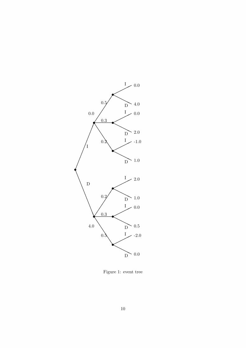
The idea of backward induction is to solve the problem from the end andworking backwards towards the initial period. Let me consider a simpleproblem of a game against nature, with a finite action set and finite supportof the stochastic process. This problem can easily be represented by an eventtree (See figure 1). It is a very simple example what is mainly due to thefact that I did not want to draw an even bigger event tree. But neverthelesslet us apply backward induction to solve this little problem. To give it aname, think of action I as ’Invest’ and D as ’Don’t invest’ and the shockare the income realization. The numbers on the lines denote the conditionalprobabilities of the shock occuring given the current history. The numbersat the end of the tree and the two numbers above and below the first twonodes are the values I want to assign for the evaluated felicity function atthese nodes7.If we now work backward we start at the last decision state and begin bydetermining the optimal behavior if the agent were at the top point. As onecan easily see, the optimal behavior there is D. If we go to the next node,again the optimal behavior is D. If we do this for all nodes in the last periodwe know the continuation value at these nodes, i.e. 4.0 at the top node, 2.0at the next node below and so on... When we now move backwards through

7You may have already noticed that we have to assume a distinct initial value for theproblem, if we want to evaluate the felicity function and do not consider cases, where theproblem is independent of the initial value. Hence we solve for a distinct problem out ofthe family of problems.

9

t¯¯¯¯¯¯¯¯¯¯

LLLLLLLLLLLL

t­­

­­

­­­

JJ

JJ

JJJ

t­­

­­

­­­

JJ

JJ

JJJ

t©©©©©

HHHHH

t©©©©©

HHHHH

t©©©©©

HHHHH

t©©©©©

HHHHH

t©©©©©

HHHHH

t©©©©©

HHHHH

0.0

4.0

0.0

4.0

0.0

2.0

-1.0

1.0

2.0

1.0

0.0

0.5

-2.0

0.0

I

D

0.5

0.3

0.2

0.2

0.3

0.5

I

DI

DI

D

I

DI

DI

D

Figure 1: event tree

10

the tree nature moves and therefore we have to determine the conditionalexpected continuation value for an agent at the node before nature moves8.The only choice left is the choice of the agent in the initial period. To de-termine the optimal behavior there we consider current payoff indicated atthe first node plus the discounted continuation value from future choices.Remember the Principle of Optimality that tells us that given any historyof shocks and choices future choices must constitute an optimal policy, i.e.maximize the expected continuation value. Hence if we evaluate the valuefunction9 for x0 we see immediately that the optimal choice in the first pe-riod is I.Hence we have by simple comparison of expected continuation values foundthe value function v(x0) for the initial state x0 and the optimal policy forevery state.Now it can be easily seen what I tried to emphasize above, namely that theoptimal policy is not only optimal in the support of the optimally controlledprocess, but also at the nodes that are never reached with positive proba-bility like all the nodes in the lower branch of the event tree in our simpleexample. This is due to the fact that when one starts solving the problemfrom the last period, one does not know ex ante which path will turn out tobe optimal because I is the optimal choice in the first period and thereforethe problem has to be solved for optimal solutions at every possible state ofthe process, i.e. also for optimal solutions in states that are never reachedonce the optimal policy is conducted. We will see later for the infinite hori-zon case, that this causes some problems for the numerical implementationif one does not impose some additional restrictions on the problem. I willdiscuss the numerical implementation of the backward induction in section6.3.

4.2 Fixed point problem

As I already mentioned above, it is a substantial step going from finite toinfinite time horizon10.Let us reconsider the problem in 8 and define the value function appropri-ately

v(x0) = maxct∞t=0

E [U(ct, xt∞t=0)|x0] (13)

8Remember that we have assumed expected utility maximization of agents9This is a slight abuse of terminology, but I will call the continuation value induced by

a certain policy value function as well although the policy function might not maximizethe expected continuation value.

10In the appendix I discuss briefly the case of a stochastic end point.

11

We can rewrite the value function as follows

E [v(x0)|x0] = maxct∞t=0

U(ct, xt∞t=0)

= maxct∞t=0

∞∑

t=0

βtE [u(ct, xt)|x0]

= maxct∞t=0

u(c0, x0) +∞∑

t=1

βtE [u(ct, xt)|x0]

= maxc0

u(c0, x0) + β maxct∞t=1

∞∑

t=1

βt−1E [u(ct, xt)|x0]

= maxc0

u(c0, x0) + βE [v(x1)|x0]

(14)

It has to be proven that this problem yields the same solution as the onein (4), but since it is not the subject of this talk I will not do it here11.Just believe me for the moment that this can be done.12. We know thatthis condition is true for every initial value and therefore it is due to thePrinciple of Optimality true for every pair of consecutive periods and wecan replace x0 by x and x1 by x′ and do the same for the control variables,then the definition of the value function becomes

v(x) = maxc

u(c, x) + βE[v(x′)|x]

(15)

This equation is also called the Bellman equation in economics and it is nolonger an algebraic equation, but it is a functional equation, because theunknown is the value function v(x). To illustrate this13 one can replace themax operator and define a new operator Ψ : V → V

v(x) = Ψ(v(x′))

This operator Ψ(·) that maps from the space of bounded functions in thespace of bounded functions can be shown to be a contraction mapping withmodulus β. This can be done using Blackwell’s sufficient conditions. Fromthe contraction mapping theorem, which is also called Banach’s fixed pointtheorem, we know that a solution exists and that is is unique. Therefore theapproach to find a solution to the Bellman equation becomes a fixed pointproblem and the algorithm to solve this problem can exploit the contractionproperty of the Bellman equation. I want to mention also that all optimalpolicy functions that solve this problem have a recursive structure.

11The interested reader can find the proof in Stokey/Lucas (1989)12There are some additional issues if the value function is unbounded, but also these

can be resolved in most cases if we choose an appropriate norm. See also Rust (2006) forfurther discussion and references.

13Let me assume for the further discussion that v(x) is a bounded function just to avoidadditional issues.

12

5 Multiplayer games and Competetive Equilibrium

So far I only considered single agent optimization problems, where an agenttries to find a feasible policy that maximizes his expected utility.Things become a bit more involved, if there are several agents or as in com-petetive equilibrium models a continuum of agents, because then the agents’optimal decisions have not only be optimal for the different states of naturebut also for the actions taken by the other agents. Therefore we have to addan outer loop to the problem to solve an additional fixed point problem.The agent’s maximization problem becomes the inner loop of the composedproblem, but the state space has to be enlarged, because it also contains thestrategies of the other players and the distribution of their characteristicslike capital holdings or age. Sometimes it might be sufficient to include somesufficient statistics about the distribution of the other agents in the statespace instead of the whole distribution.The algorithm to solve the composed problem goes back and forth betweenthe two problems until it converges to a set of policies/strategies such thatthe policies/strategies of agents are optimal given the other players poli-cies/strategies, i.e. the strategies are mutual best responses, and the as-sumed behavior of the other agents by agents solving their maximizationproblem is the behavior that the other agents will choose in the end. Thisis also called rational expectations in economics.Furthermore we require that in a competetive equilibrium these optimalstrategies yield market clearing at given prices.There is an additional issue arising in the multiple agent settings, becausethere might be a multiplicity of equilibria. Although there are multiple op-timal solutions to the single agent optimization problem as discussed above,the problem in the multiple agent setting is that the agents might have dif-ferent payoffs across different equilibria.There are especially in game theory a variety of equilibrium refinements torule out some of the equilirbia, like the concept of Markov-perfect equilibria,but I do not want to discuss them here.

6 Numerical Methods

After I have presented the theory underlying Dynamic Programming I amnow going to present some numerical implementations to solve the generalproblem based on this theory. First I consider the finite horizon case thatwe solved using backward induction and then I discuss several closely relatedapproaches to solve the infinite horizon problem.

13

6.1 Function approximation methods

It is important to distinguish two concepts for function approximation. Oneapproach which I will call the local approach tries to approximate the func-tion by a large number of function values over a fine grid and then approx-imate the function by interpolation between these function values.The other approach I will call the global approach14 tries to approximate thefunction by a set of basis functions whose shape is governed by a finite setof parameters.

6.2 Grid Choice

In many problems the state space X and the feasible set for the control Γ(X)contain a continuum of elements.Since the numerical routine can not handle infinite dimensional objects di-rectly, some discretization is needed. Different methods have been proposedof how to do this discretezation. From the above discussion it should benoted that the state space might contain infinite dimensional objects likethe distribution functions or best response functions of other plyaers. Theseobjects have to be either discretized using the methods below or parame-terized using the methods described later. I will call the set of discretizedvalues the grid.The problem of grid choice is discussed here only briefly and not in theextent it might require. The problem is closely related to the issue of nu-merical integration, because the same problems arise there. Since I do nothave the time I will not cover this topic here and the interested reader isreferred some book on numerical methods like Judd (1998).The outline of the methods I give here is very basic and by no means ex-haustive.

6.2.1 Equally spaced grids

The first approach is to choose an equally spaced grid in each dimensionof the single state space and then form the Cartisian product of the stategrids. This approach has the problem, that the set of grid points growsexponentially in the grid points of the single state directions and this iscalled the Curse of Dimensionality and is maybe the major drawback ofDynamic Programming .

6.2.2 Random grid

An alternaitve would be to choose not grids in each state direction butdo random sampling in the state space, i.e. we draw from some random

14I choose this term to distinguish it from the local approach, although it might be a bitmisleading, because we still approximate the function only on a subset of the domain.

14

distribution the elements of the state space. Here the algorithm designercan set the number of grid points. If this is done appropriately it can helpto get around the Curse of Dimensionality .

6.2.3 Adaptive grids

A third possibility I want to present briefly is the possibility of an adaptivegrid choice. The idea of this approach is to choose a coarse grid in thebeginnig and solve the problem once on for this coarse grid. After thesolution has been obtained there are successively grid points added at regionsin the state space, where the function seems to have a lot of curvature.

6.2.4 Interpolation

The function approximation by a finite number function values over a set ofgrid points has the problem that the function is still unknown at most of thepoints in its support. Therefore one needs methods to derive the functionvalue at points, which are not in the grid. This is done using interpolationmethods.Since these nodes are on Dynamic Programming and are supposed to beonly an introduction I am not going to discuss interpolation methods hereand refer to Judd(1998).

6.3 Backward induction algorithm

Backward induction is an easy to implement algorithm. The only issue thatarises is in the case of continuous state and control variables. To implementcontinuous variables on a computer, one has to choose some kind of dis-cretization. The other issue is the Curse of Dimensionality . I will discussthese problems in section 7.Suppose we are able to appropriately take care of these two issues, thenthe backward induction algorithm consists mainly of a grid search over thefeasible set of policies for each state.

15

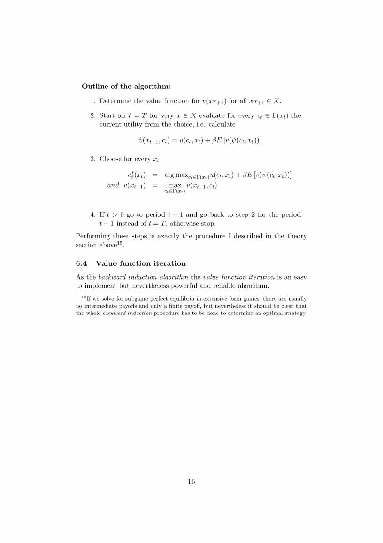
Outline of the algorithm:

1. Determine the value function for v(xT+1) for all xT+1 ∈ X.

2. Start for t = T for very x ∈ X evaluate for every ct ∈ Γ(xt) thecurrent utility from the choice, i.e. calculate

v(xt−1, ct) = u(ct, xt) + βE [v(ψ(ct, xt))]

3. Choose for every xt

c∗t (xt) = arg maxct∈Γ(xt)u(ct, xt) + βE [v(ψ(ct, xt))]and v(xt−1) = max

ct∈Γ(xt)v(xt−1, ct)

4. If t > 0 go to period t − 1 and go back to step 2 for the periodt− 1 instead of t = T , otherwise stop.

Performing these steps is exactly the procedure I described in the theorysection above15.

6.4 Value function iteration

As the backward induction algorithm the value function iteration is an easyto implement but nevertheless powerful and reliable algorithm.

15If we solve for subgame perfect equilibria in extensive form games, there are usuallyno intermediate payoffs and only a finite payoff, but nevertheless it should be clear thatthe whole backward induction procedure has to be done to determine an optimal strategy.

16

Outline of the algorithm:

1. Choose a convergence criterion ε for ‖vi(x)− vi−1(x)‖ < ε

2. Start with an initial guess for the value function v0(x), e.g. v0(x) =0

3. For very x ∈ X evaluate for every c ∈ Γ(x) the current utilityfrom the choice if the value function vi(x) were the correct valuefunction, i.e. calculate

v(xt−1, ct) = u(c, x) + βE [vi(ψ(c, x))]

4. Choose for every x

c∗(x) = arg maxc∈Γ(x)u(c, x) + βE [vi(ψ(c, x))]and vi+1(x) = max

c∈Γ(x)v(xt−1, ct)

5. Check convergence. If the value function has not yet convergedgo back to step 3 and use vi+1(x) as guess for the value function,otherwise stop.

It relies on the contraction mapping property of the Bellman equation in(15). Since the Bellman equation has an unique fixed point this algorithmwill converge to the true solution and uses the method of successive approx-imations. Starting from v0(x) it can be shown that

limt→∞Ψt (v0(x)) = v(x)

Moreover it can be shown that

‖v(x)− vi(x)‖ ≤ 11− β

‖vi+1(x)− vi(x)‖

The inequality can also be used to pick the stopping criterion.There is a nice intuition why this approach works, namely because we assumethat agents discount future utility, the effect of future periods on the valuefunction decreases with the distance of the future date from the currentdate of the decision. Remember that we have β ∈ (0, 1) and thereforelimt→∞ βt = 0. There will be some date in the future where the effect onthe value function is almost neglectable. If one compares the value functioniteration to the backward induction algorithm one sees that essentially thesame is done, i.e. starting from some period and going back in time, but thistime the index is i and not t but otherwise the same procedure is conducted.The only difference is that this time the algorithm does not stop in t = 0

17

but iterates until the value function has converged. This can be thought ofas increasing the agent’s time horizon until it is almost infinity. Thereforewe have approximated the infinite time horizon by a finite time horizon thatis sufficiently large.

6.5 Howard’s improvement algorithm

The Howard’s improvement algorithm is also known as policy function it-eration. It works similar to the value function iteration, but this time theguess is for the optimal policy.First notice that a policy function can also be represented by a transitionfunction. It is a mutation of the transition function of the stochastic process,because next period’s states are a function of the current state and the con-trol this period. If one changes the control this period, it just shifts theprobability distribution next period. So if we guess a policy c0(x), we canrepresent it by a transition function Ω(c) and we get the following Bellmanequation

v(x) = u(c(x), x) + βΩ(c)v(x)

But this can be easily solved16 for v(x)

v(x) = (I − βΩ(c))−1 u(c(x), x)

and we get an implied value function v(x). With this trick at hand I cannow outline the algorithm.

16The inverse of (I − βΩ(c)) exists always because the matrix is diagonally dominantand therefore the inverse exists.

18

Outline of the algorithm:

1. Choose a convergence criterion ε for ‖ci(x)− ci−1(x)‖ < ε

2. Start with an initial guess for the policy function c0(x), that isfeasible. Derive the implied transition function Ω(c).

3. Perform the value function updating

v(x) = (I − βΩ(c))−1 u(c(x), x)

4. For very x ∈ X evaluate for every c ∈ Γ(x) the current utilityfrom the choice if the value function v(x) were the correct valuefunction, i.e. calculate

v(xt−1, ct) = u(c, x) + βE [v(ψ(c, x))]

5. Choose for every x

ci+1(x) = arg maxc∈Γ(x)u(c, x) + βE [vi(ψ(c, x))]and v(x) = max

c∈Γ(x)v(xt−1, ct)

6. Check convergence. If the policy function has not yet convergedgo back to step 2 and use ci+1(x) as guess for the policy function,otherwise stop.

The advantage of the policy function iteration algorithm is that it in generalconverges faster. If it converges faster than the value function iterationalgorithm depends on the modulus of the contraction mapping. If it is closeto one the policy function iteration is much faster, but the time advantagedecreases with decreasing modulus and the value function iteration mighteven become faster, because it does not require any matrix inversion.

6.6 Modified policy function iteration

An other method used in applied work, that has proven to yield a substantialincrease in convergence speed without requiring matix inversion, is what Iwill call modified policy function iteration.The algorithm works along the same lines as the value function iteration,but instead of just one updating step as before it does several updating stepsonce a new policy has been determined.It does not like in the Howard’s improvement algorithm compute the inverseand uses the updating formula to get a new policy, but it just applies the newpolicy several times. Therefore we add an additional step to the algorithm

19

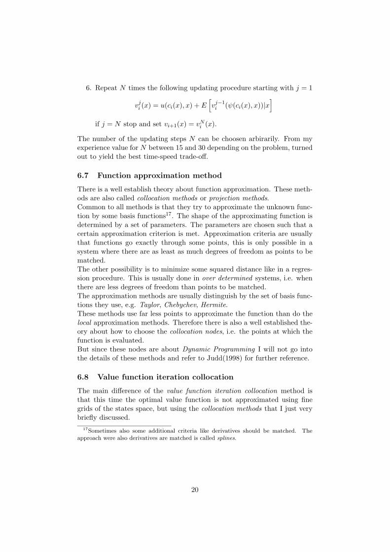
6. Repeat N times the following updating procedure starting with j = 1

vji (x) = u(ci(x), x) + E

[vj−1i (ψ(ci(x), x))|x

]

if j = N stop and set vi+1(x) = vNi (x).

The number of the updating steps N can be choosen arbirarily. From myexperience value for N between 15 and 30 depending on the problem, turnedout to yield the best time-speed trade-off.

6.7 Function approximation method

There is a well establish theory about function approximation. These meth-ods are also called collocation methods or projection methods.Common to all methods is that they try to approximate the unknown func-tion by some basis functions17. The shape of the approximating function isdetermined by a set of parameters. The parameters are chosen such that acertain approximation criterion is met. Approximation criteria are usuallythat functions go exactly through some points, this is only possible in asystem where there are as least as much degrees of freedom as points to bematched.The other possibility is to minimize some squared distance like in a regres-sion procedure. This is usually done in over determined systems, i.e. whenthere are less degrees of freedom than points to be matched.The approximation methods are usually distinguish by the set of basis func-tions they use, e.g. Taylor, Chebychev, Hermite.These methods use far less points to approximate the function than do thelocal approximation methods. Therefore there is also a well established the-ory about how to choose the collocation nodes, i.e. the points at which thefunction is evaluated.But since these nodes are about Dynamic Programming I will not go intothe details of these methods and refer to Judd(1998) for further reference.

6.8 Value function iteration collocation

The main difference of the value function iteration collocation method isthat this time the optimal value function is not approximated using finegrids of the states space, but using the collocation methods that I just verybriefly discussed.

17Sometimes also some additional criteria like derivatives should be matched. Theapproach were also derivatives are matched is called splines.

20

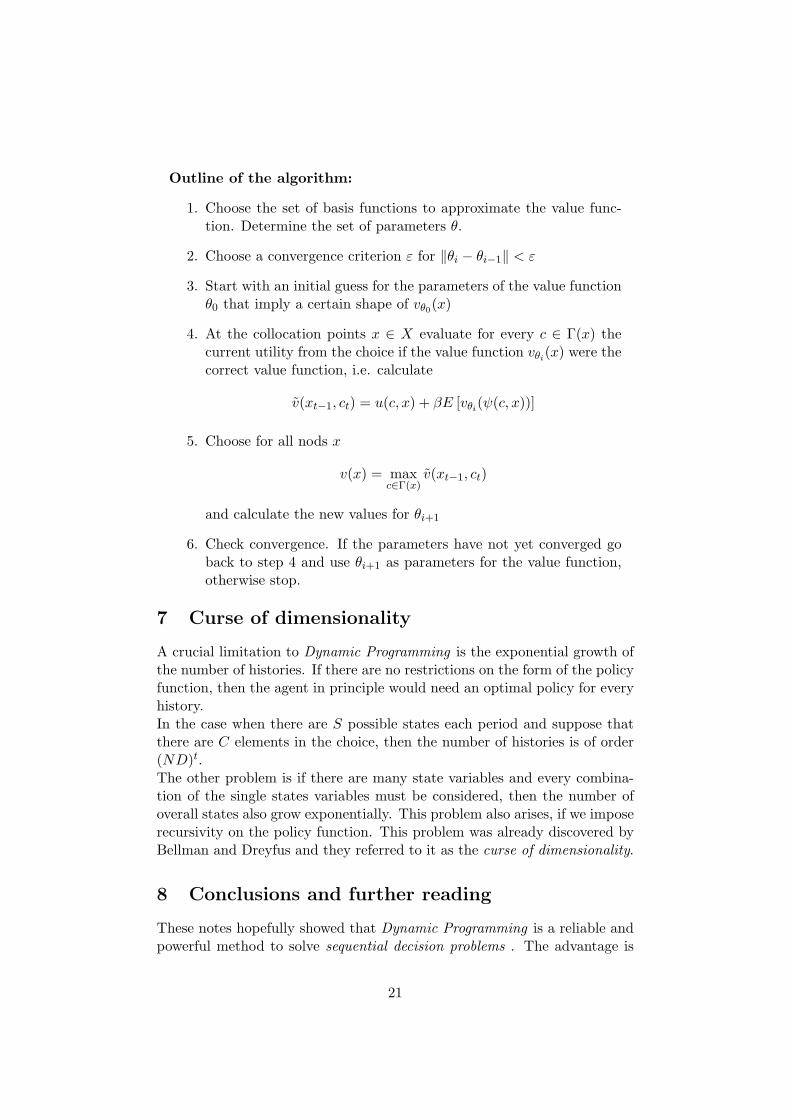
Outline of the algorithm:

1. Choose the set of basis functions to approximate the value func-tion. Determine the set of parameters θ.

2. Choose a convergence criterion ε for ‖θi − θi−1‖ < ε

3. Start with an initial guess for the parameters of the value functionθ0 that imply a certain shape of vθ0(x)

4. At the collocation points x ∈ X evaluate for every c ∈ Γ(x) thecurrent utility from the choice if the value function vθi(x) were thecorrect value function, i.e. calculate

v(xt−1, ct) = u(c, x) + βE [vθi(ψ(c, x))]

5. Choose for all nods x

v(x) = maxc∈Γ(x)

v(xt−1, ct)

and calculate the new values for θi+1

6. Check convergence. If the parameters have not yet converged goback to step 4 and use θi+1 as parameters for the value function,otherwise stop.

7 Curse of dimensionality

A crucial limitation to Dynamic Programming is the exponential growth ofthe number of histories. If there are no restrictions on the form of the policyfunction, then the agent in principle would need an optimal policy for everyhistory.In the case when there are S possible states each period and suppose thatthere are C elements in the choice, then the number of histories is of order(ND)t.The other problem is if there are many state variables and every combina-tion of the single states variables must be considered, then the number ofoverall states also grow exponentially. This problem also arises, if we imposerecursivity on the policy function. This problem was already discovered byBellman and Dreyfus and they referred to it as the curse of dimensionality.

8 Conclusions and further reading

These notes hopefully showed that Dynamic Programming is a reliable andpowerful method to solve sequential decision problems . The advantage is

21

that it has a well established theory.Especially the easy incorporation of uncertainty make it a widely used ap-proach in economics. Dynamic Programming can be applied in a large va-riety of economic problems, e.g. general equilibrium theory, industrial orga-nization, game theory or mechanism design.Although I emphasized the numerical application in these notes, DynamicProgramming is also of theoretical interest for economic research.Numerically Dynamic Programming is an easy and straightforward to im-plement method, that yields accurate results and is insensible to numericalinaccuracy.Finally I should mention that these notes are only a short introduction toDynamic Programming and are by far not an exhaustive introduction to allissues of Dynamic Programming . People how want to apply the methodsshould also be familiar with the related fields of numerical work like functionapproximation or integration.

References

[1] Richard Bellman. Dynamic Programming. Princeton University Press,1957.

[2] Kenneth L. Judd. Numerical Methods in Economics. Cambridge Uni-versity Press, 1998.

[3] John Rust. Dynamic programming. Entry for consideration by the NewPalgrave Dictionary of Economics.

[4] Nancy L. Stokey and Robert E. Lucas. Recursive Methods in EconomicDynamics. Harvard University Press, 1989.

22

A Extensive form games

An extensive form game Ψ(I, T , Sii∈I , Ξii∈I , ui(·)i∈I , φ(S)) is acollection of players indexed by i ∈ I, a time structure for players’ actionsT , strategy sets Si, information sets Ξi and a payoff function for each playerthat maps histories of actions into payoffs ui : ×i∈I ×t∈T Si → R.

These games are commonly described by a game tree.

B Markov Chain

Let us assume that Xt is a random variable with finite support. Let us denotethe probability of Xt = xt given the history xt−1 = xt−1, xt−2, . . . , x0as Π(xt|xt−1). The stochastic process is a Markov chain if Π(xt|xt−1) =Π(xt|xt−1), i.e. the probability of xt only depends on the realization of thelast period xt−1.

C Undertermined end time

These problems can numerically be treated like finite horizon problems. Theonly restriction one has to impose is that there is a T such that survival prob-ability is zero. But this assumption does not seem to be too unreasonable.The only difference is that we now have an additional survival probabilityentering the problem, since it is uncertain, if the agent will survive and bestill alive in the next period. The way to adjust for that is that we multiplythe transition probabilities by a survival probability. Therefore let me definethe discounted transition probability by

Π(st+1|st) := ρt+1Π(st+1|st)

where Π(st+1|st) denotes the conditional probability of going from state st tostate st+1 and ρt+1 denotes the survival probability from period t to t+1. Wecan now solve the problem as before, but use the transition probabilities ˜Π(·)instead of Π(·). But keep in mind that the discounted transition probabilitywill not sum to 1 anymore but to ρ.

23