A Closed-Form Solution for Options with Stochastic

A Closed-Form Solution forOptions with StochasticVolatility with Applicationsto Bond and CurrencyOptionsSteven L. HestonYale University

I use a new technique to derive a closed-form solu-tion for the price of a European call option on anasset with stochastic volatility. The model allowsarbitrary correlation between volatility and spot-asset returns. I introduce stochastic interest ratesand show how to apply the model to bond optionsand foreign currency options. Simulations showthat correlation between volatility and the spotasset’s price is important for explaining returnskewness and strike-price biases in the Black-Scholes (1973) model. The solution technique isbased on characteristic functions and can beapplied to other problems.

Many plaudits have been aptly used to describe Blackand Scholes’ (1973) contribution to option pricingtheory. Despite subsequent development of optiontheory, the original Black-Scholes formula for a Euro-pean call option remains the most successful andwidely used application. This formula is particularlyuseful because it relates the distribution of spot returns

I thank Hans Knoch for computational assistance. I am grateful for thesuggestions of Hyeng Keun (the referee) and for comments by participantsat a 1992 National Bureau of Economic Research seminar and the Queen’sUniversity 1992 Derivative Securities Symposium. Any remaining errors aremy responsibility. Address correspondence to Steven L. Heston, Yale Schoolof Organization and Management, 135 Prospect Street, New Haven, CT 06511.

The Review of Financial Studies 1993 Volume 6, number 2, pp. 327-343© 1993 The Review of Financial Studies 0893-9454/93/$1.50

The Review of Financial Studies / v 6 n 2 1993

to the cross-sectional properties of option prices. In this article, I

generalize the model while retaining this feature.

Although the Black–Scholes formula is often quite successful in

explaining stock option prices [Black and Scholes (1972)], it does

have known biases [Rubinstein (1985)]. Its performance also is sub-

stantially worse on foreign currency options [Melino and Turnbull(1990, 1991), Knoch (1992)]. This is not surprising, since the Black-

Scholes model makes the strong assumption that (continuously com-

pounded) stock returns are normally distributed with known mean

and variance. Since the Black–Scholes formula does not depend on

the mean spot return, it cannot be generalized by allowing the mean

to vary. But the variance assumption is somewhat dubious. Motivated

by this theoretical consideration, Scott (1987), Hull and White (1987),

and Wiggins (1987) have generalized the model to allow stochastic

volatility. Melino and Turnbull (1990, 1991) report that this approach

is successful in explaining the prices of currency options. These

papers have the disadvantage that their models do not have closed-

form solutions and require extensive use of numerical techniques to

solve two-dimensional partial differential equations. Jarrow and

Eisenberg (1991) and Stein and Stein (1991) assume that volatility

is uncorrelated with the spot asset and use an average of Black-

Scholes formula values over different paths of volatility. But since this

approach assumes that volatility is uncorrelated with spot returns, it

cannot capture important skewness effects that arise from such cor-

relation. I offer a model of stochastic volatility that is not based on

the Black-Scholes formula. I t provides a closed-form solution for the

price of a European call option when the spot asset is correlated with

volatility, and it adapts the model to incorporate stochastic interest

rates. Thus, the model can be applied to bond options and currency

options.

1. Stochastic Volatility Model

We begin by assuming that the spot asset at time t follows the diffusion

(1)

where is a Wiener process. If the volatility follows an Ornstein–Uhlenbeck process [e.g., used by Stein and Stein (1991)],

dS (t) dt + ,

then Ito’s lemma shows that the variance follows the process

328

(t)

Closed-Form Solution for Options with Stochastic Volatility

(3)

This can be written as the familiar square-root process [used by Cox,Ingersoll, and Ross (1985)]

(4)

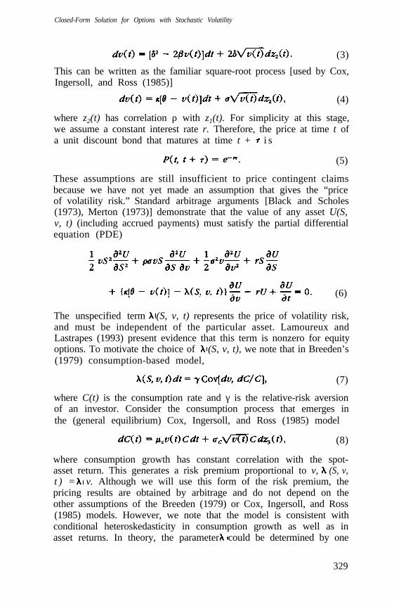
where z2(t) has correlation ρ with z1(t). For simplicity at this stage,we assume a constant interest rate r. Therefore, the price at time t ofa unit discount bond that matures at time t + i s

(5)

These assumptions are still insufficient to price contingent claimsbecause we have not yet made an assumption that gives the “priceof volatility risk.” Standard arbitrage arguments [Black and Scholes(1973), Merton (1973)] demonstrate that the value of any asset U(S,v, t) (including accrued payments) must satisfy the partial differentialequation (PDE)

(6)

The unspecified term (S, v, t) represents the price of volatility risk,and must be independent of the particular asset. Lamoureux andLastrapes (1993) present evidence that this term is nonzero for equityoptions. To motivate the choice of (S, v, t), we note that in Breeden’s(1979) consumption-based model,

(7)

where C(t) is the consumption rate and γ is the relative-risk aversionof an investor. Consider the consumption process that emerges inthe (general equilibrium) Cox, Ingersoll, and Ross (1985) model

(8)

where consumption growth has constant correlation with the spot-asset return. This generates a risk premium proportional to v, (S, v,t ) = v. Although we will use this form of the risk premium, thepricing results are obtained by arbitrage and do not depend on theother assumptions of the Breeden (1979) or Cox, Ingersoll, and Ross(1985) models. However, we note that the model is consistent withconditional heteroskedasticity in consumption growth as well as inasset returns. In theory, the parameter could be determined by one

329

The Review of Financial Studies/ v 6 n 2 1993

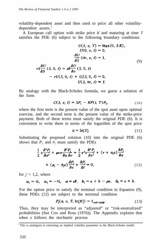
volatility-dependent asset and then used to price all other volatility-dependent assets.1

A European call option with strike price K and maturing at time Tsatisfies the PDE (6) subject to the following boundary conditions:

(9)

By analogy with the Black-Scholes formula, we guess a solution ofthe form

( 1 0 )

where the first term is the present value of the spot asset upon optimalexercise, and the second term is the present value of the strike-pricepayment. Both of these terms must satisfy the original PDE (6). It isconvenient to write them in terms of the logarithm of the spot price

(11)

Substituting the proposed solution (10) into the original PDE (6)shows that P1 and P2 must satisfy the PDEs

(12)

for j = 1,2, where

For the option price to satisfy the terminal condition in Equation (9),these PDEs (12) are subject to the terminal condition

(13)

Thus, they may be interpreted as “adjusted” or “risk-neutralized”probabilities (See Cox and Ross (1976)). The Appendix explains thatwhen x follows the stochastic process

1 This is analogous to extracting an implied volatility parameter in the Black-Scholes model.

330


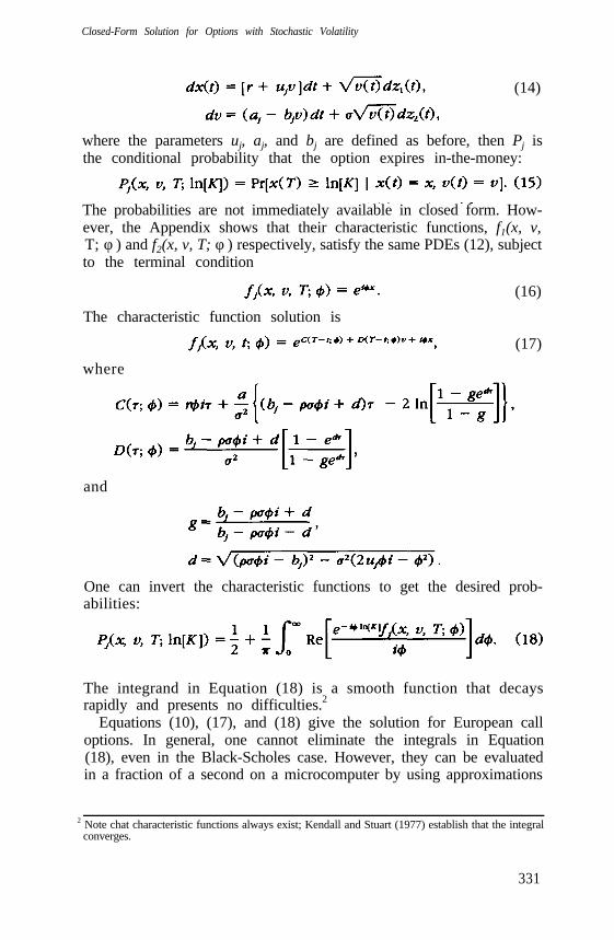
(14)

where the parameters uj, aj, and bj are defined as before, then Pj isthe conditional probability that the option expires in-the-money:

The probabilities are not immediately available in closed form. How-ever, the Appendix shows that their characteristic functions, f1(x, v,T; φ ) and f2(x, v, T; φ ) respectively, satisfy the same PDEs (12), subjectto the terminal condition

The characteristic function solution is

where

(16)

(17)

and

One can invert the characteristic functions to get the desired prob-abilities:

The integrand in Equation (18) is a smooth function that decaysrapidly and presents no difficulties.2

Equations (10), (17), and (18) give the solution for European calloptions. In general, one cannot eliminate the integrals in Equation(18), even in the Black-Scholes case. However, they can be evaluatedin a fraction of a second on a microcomputer by using approximations

2 Note chat characteristic functions always exist; Kendall and Stuart (1977) establish that the integralconverges.

331


similar to the standard ones used to evaluate cumulative normal prob-abilities.3

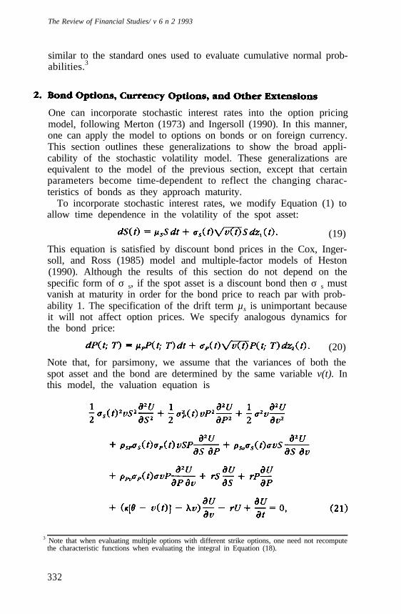
One can incorporate stochastic interest rates into the option pricingmodel, following Merton (1973) and Ingersoll (1990). In this manner,one can apply the model to options on bonds or on foreign currency.This section outlines these generalizations to show the broad appli-cability of the stochastic volatility model. These generalizations areequivalent to the model of the previous section, except that certainparameters become time-dependent to reflect the changing charac-teristics of bonds as they approach maturity.

To incorporate stochastic interest rates, we modify Equation (1) toallow time dependence in the volatility of the spot asset:

(19)

This equation is satisfied by discount bond prices in the Cox, Inger-soll, and Ross (1985) model and multiple-factor models of Heston(1990). Although the results of this section do not depend on thespecific form of σ s, if the spot asset is a discount bond then σ s mustvanish at maturity in order for the bond price to reach par with prob-ability 1. The specification of the drift term µ s is unimportant becauseit will not affect option prices. We specify analogous dynamics forthe bond price:

(20)

Note that, for parsimony, we assume that the variances of both thespot asset and the bond are determined by the same variable v(t). Inthis model, the valuation equation is

3 Note that when evaluating multiple options with different strike options, one need not recomputethe characteristic functions when evaluating the integral in Equation (18).

332


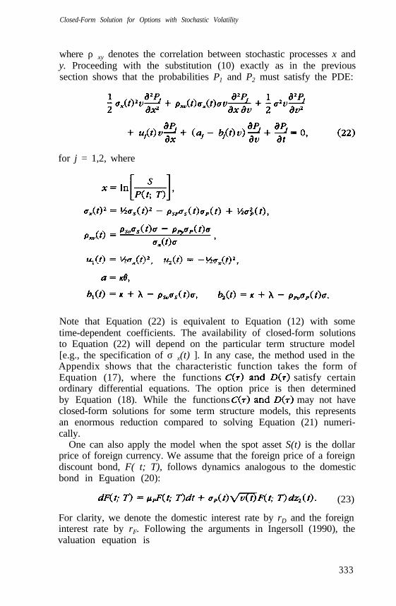
where ρ xy denotes the correlation between stochastic processes x andy. Proceeding with the substitution (10) exactly as in the previoussection shows that the probabilities P1 and P2 must satisfy the PDE:

for j = 1,2, where

Note that Equation (22) is equivalent to Equation (12) with sometime-dependent coefficients. The availability of closed-form solutionsto Equation (22) will depend on the particular term structure model[e.g., the specification of σ x(t) ]. In any case, the method used in theAppendix shows that the characteristic function takes the form ofEquation (17), where the functions satisfy certainordinary differential equations. The option price is then determinedby Equation (18). While the functions may not haveclosed-form solutions for some term structure models, this representsan enormous reduction compared to solving Equation (21) numeri-cally.

One can also apply the model when the spot asset S(t) is the dollarprice of foreign currency. We assume that the foreign price of a foreigndiscount bond, F( t; T), follows dynamics analogous to the domesticbond in Equation (20):

(23)

For clarity, we denote the domestic interest rate by rD and the foreigninterest rate by rF. Following the arguments in Ingersoll (1990), thevaluation equation is

333


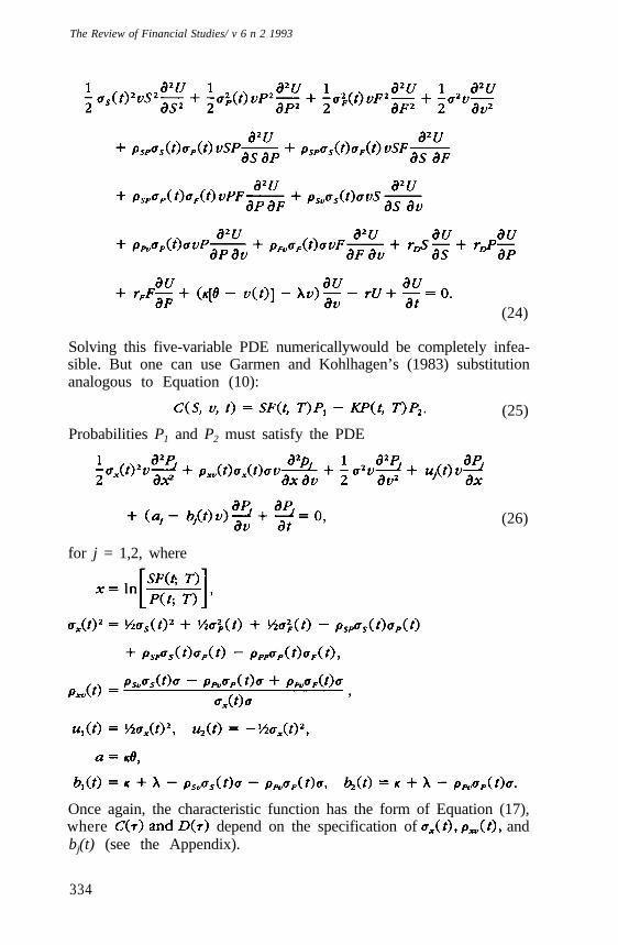
(24)

Solving this five-variable PDE numericallywould be completely infea-sible. But one can use Garmen and Kohlhagen’s (1983) substitutionanalogous to Equation (10):

Probabilities P1 and P2 must satisfy the PDE

(25)

(26)

for j = 1,2, where

Once again, the characteristic function has the form of Equation (17),where depend on the specification of andbj(t) (see the Appendix).

334


Although the stochastic interest rate models of this section aretractable, they would be more complicated to estimate than the sim-pler model of the previous section. For short-maturity options onequities, any increase in accuracy would likely be outweighed by theestimation error introduced by implementing a more complicatedmodel. As option maturities extend beyond one year, however, theinterest rate effects can become more important [Koch (1992)]. Themore complicated models illustrate how the stochastic volatility modelcan be adapted to a variety of applications. For example, one couldvalue U.S. options by adding on the early exercise approximation ofBarone-Adesi and Whalley (1987). The solution technique has otherapplications, too. See the Appendix for application to Stein and Stein’s(1991) model (with correlated volatility) and see Bates (1992) forapplication to jump-diffusion processes.

3. Effects of the Stochastic Volatility Model Options Prices

In this section, I examine the effects of stochastic volatility on optionsprices and contrast results with the Black-Scholes model. Many effectsare related to the time-series dynamics of volatility. For example, ahigher variance v(t) raises the prices of all options, just as it does inthe Black-Scholes model. In the risk-neutralized pricing probabili-ties, the variance follows a square-root process

where

(27)

and

We analyze the model in terms of this risk-neutralized volatility pro-cess instead of the “true” process of Equation (4), because the risk-neutralized process exclusively determines prices.4 The variance driftstoward a long-run mean of θ *, with mean-reversion speed determinedby K*. Hence, an increase in the average variance θ * increases theprices of options. The mean reversion then determines the relativeweights of the current variance and the long-run variance on optionprices. When mean reversion is positive, the variance has a steady-state distribution [Cox, Ingersoll, and Ross (1985)] with mean θ *.Therefore, spot returns over long periods will have asymptoticallynormal distributions, with variance per unit of time given by θ *.Consequently, the Black-Scholes model should tend to work wellfor long-term options. However, it is important to realize that the

4 This occurs for exactly the same reason that the Black-Scholes formula does not depend on themean stock return. See Heston (1992) for a theoretical analysis that explains when parameters dropout of option prices.

335


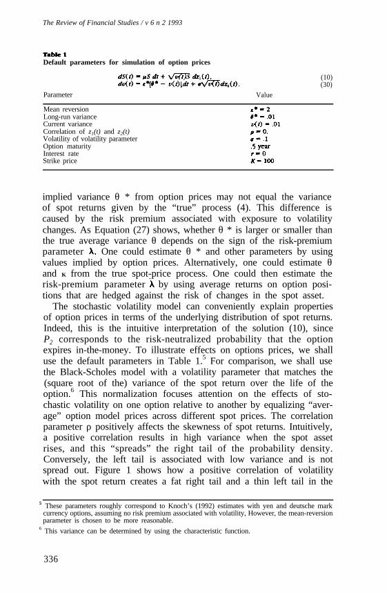
Default parameters for simulation of option prices

(10)(30)

Parameter Value

Mean reversionLong-run varianceCurrent varianceCorrelation of z1(t) and z2(t)Volatility of volatility parameterOption maturityInterest rateStrike price

implied variance θ * from option prices may not equal the varianceof spot returns given by the “true” process (4). This difference iscaused by the risk premium associated with exposure to volatilitychanges. As Equation (27) shows, whether θ * is larger or smaller thanthe true average variance θ depends on the sign of the risk-premiumparameter One could estimate θ * and other parameters by usingvalues implied by option prices. Alternatively, one could estimate θand K from the true spot-price process. One could then estimate therisk-premium parameter by using average returns on option posi-tions that are hedged against the risk of changes in the spot asset.

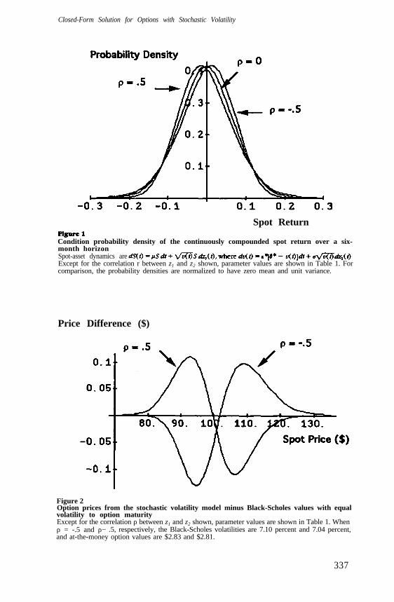
The stochastic volatility model can conveniently explain propertiesof option prices in terms of the underlying distribution of spot returns.Indeed, this is the intuitive interpretation of the solution (10), sinceP2 corresponds to the risk-neutralized probability that the optionexpires in-the-money. To illustrate effects on options prices, we shalluse the default parameters in Table 1.5 For comparison, we shall usethe Black-Scholes model with a volatility parameter that matches the(square root of the) variance of the spot return over the life of theoption.6 This normalization focuses attention on the effects of sto-chastic volatility on one option relative to another by equalizing “aver-age” option model prices across different spot prices. The correlationparameter ρ positively affects the skewness of spot returns. Intuitively,a positive correlation results in high variance when the spot assetrises, and this “spreads” the right tail of the probability density.Conversely, the left tail is associated with low variance and is notspread out. Figure 1 shows how a positive correlation of volatilitywith the spot return creates a fat right tail and a thin left tail in the

5 These parameters roughly correspond to Knoch’s (1992) estimates with yen and deutsche markcurrency options, assuming no risk premium associated with volatility, However, the mean-reversionparameter is chosen to be more reasonable.

6 This variance can be determined by using the characteristic function.

336


Spot Return

Condition probability density of the continuously compounded spot return over a six-month horizonSpot-asset dynamics areExcept for the correlation r between z1 and z2 shown, parameter values are shown in Table 1. Forcomparison, the probability densities are normalized to have zero mean and unit variance.

Price Difference ($)

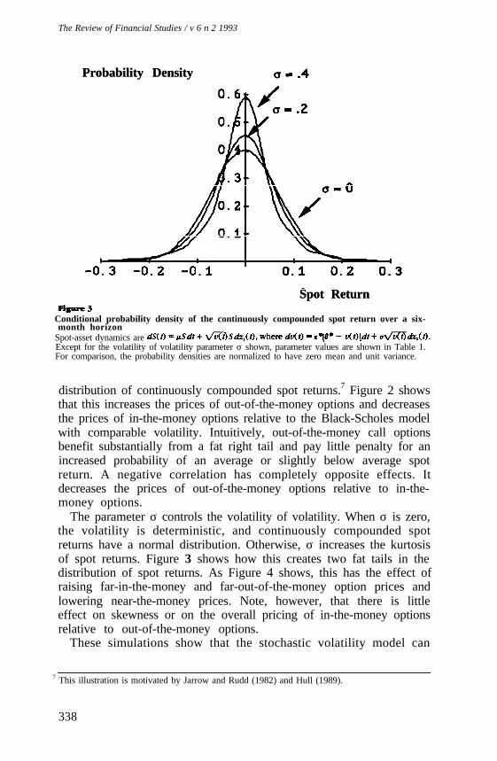
Figure 2Option prices from the stochastic volatility model minus Black-Scholes values with equalvolatility to option maturityExcept for the correlation ρ between z1 and z2 shown, parameter values are shown in Table 1. Whenρ = -.5 and ρ− .5, respectively, the Black-Scholes volatilities are 7.10 percent and 7.04 percent,and at-the-money option values are $2.83 and $2.81.

337


Probability DensityProbability Density

Spot ReturnSpot Return

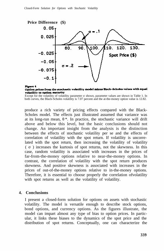
Conditional probability density of the continuously compounded spot return over a six-

Spot-asset dynamics areExcept for the volatility of volatility parameter σ shown, parameter values are shown in Table 1.For comparison, the probability densities are normalized to have zero mean and unit variance.

month horizon

distribution of continuously compounded spot returns.7 Figure 2 showsthat this increases the prices of out-of-the-money options and decreasesthe prices of in-the-money options relative to the Black-Scholes modelwith comparable volatility. Intuitively, out-of-the-money call optionsbenefit substantially from a fat right tail and pay little penalty for anincreased probability of an average or slightly below average spotreturn. A negative correlation has completely opposite effects. Itdecreases the prices of out-of-the-money options relative to in-the-money options.

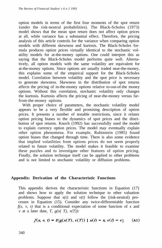
The parameter σ controls the volatility of volatility. When σ is zero,the volatility is deterministic, and continuously compounded spotreturns have a normal distribution. Otherwise, σ increases the kurtosisof spot returns. Figure 3 shows how this creates two fat tails in thedistribution of spot returns. As Figure 4 shows, this has the effect ofraising far-in-the-money and far-out-of-the-money option prices andlowering near-the-money prices. Note, however, that there is littleeffect on skewness or on the overall pricing of in-the-money optionsrelative to out-of-the-money options.

These simulations show that the stochastic volatility model can

7 This illustration is motivated by Jarrow and Rudd (1982) and Hull (1989).

338


Price Difference ($)

Except for the volatility of volatility parameter σ shown, parameter values are shown in Table 1. Inboth curves, the Black-Scholes volatility is 7.07 percent and the at-the-money option value is 12.82.

produce a rich variety of pricing effects compared with the Black-Scholes model. The effects just illustrated assumed that variance wasat its long-run mean, θ *. In practice, the stochastic variance will driftabove and below this level, but the basic conclusions should notchange. An important insight from the analysis is the distinctionbetween the effects of stochastic volatility per se and the effects ofcorrelation of volatility with the spot return. If volatility is uncorre-lated with the spot return, then increasing the volatility of volatility( σ ) increases the kurtosis of spot returns, not the skewness. In thiscase, random volatility is associated with increases in the prices offar-from-the-money options relative to near-the-money options. Incontrast, the correlation of volatility with the spot return producesskewness. And positive skewness is associated with increases in theprices of out-of-the-money options relative to in-the-money options.Therefore, it is essential to choose properly the correlation ofvolatilitywith spot returns as well as the volatility of volatility.

4. Conclusions

I present a closed-form solution for options on assets with stochasticvolatility. The model is versatile enough to describe stock options,bond options, and currency options. As the figures illustrate, themodel can impart almost any type of bias to option prices. In partic-ular, it links these biases to the dynamics of the spot price and the
distribution of spot returns. Conceptually, one can characterize the
339


A

option models in terms of the first four moments of the spot return(under the risk-neutral probabilities). The Black-Scholes (1973)model shows that the mean spot return does not affect option pricesat all, while variance has a substantial effect. Therefore, the pricinganalysis of this article controls for the variance when comparing optionmodels with different skewness and kurtosis. The Black-Scholes for-mula produces option prices virtually identical to the stochastic vol-atility models for at-the-money options. One could interpret this assaying that the Black-Scholes model performs quite well. Alterna-tively, all option models with the same volatility are equivalent forat-the-money options. Since options are usually traded near-the-money,this explains some of the empirical support for the Black-Scholesmodel. Correlation between volatility and the spot price is necessaryto generate skewness. Skewness in the distribution of spot returnsaffects the pricing of in-the-money options relative to-out-of-the moneyoptions. Without this correlation, stochastic volatility only changesthe kurtosis. Kurtosis affects the pricing of near-the-money versus far-from-the-money options.

With proper choice of parameters, the stochastic volatility modelappears to be a very flexible and promising description of optionprices. It presents a number of testable restrictions, since it relatesoption pricing biases to the dynamics of spot prices and the distri-bution of spot returns. Knoch (1992) has successfully used the modelto explain currency option prices. The model may eventually explainother option phenomena. For example, Rubinstein (1985) foundoption biases that changed through time. There is also some evidencethat implied volatilities from options prices do not seem properlyrelated to future volatility. The model makes it feasible to examinethese puzzles and to investigate other features of option pricing.Finally, the solution technique itself can be applied to other problemsand is not limited to stochastic volatility or diffusion problems.

ppendix: Derivation of the Characteristic Functions

This appendix derives the characteristic functions in Equation (17)and shows how to apply the solution technique to other valuationproblems. Suppose that x(t) and v(t) follow the (risk-neutral) pro-cesses in Equation (15). Consider any twice-differentiable functionf(x, v, t) that is a conditional expectation of some function of x andv at a later date, T, g(x( T), v(T)):

340


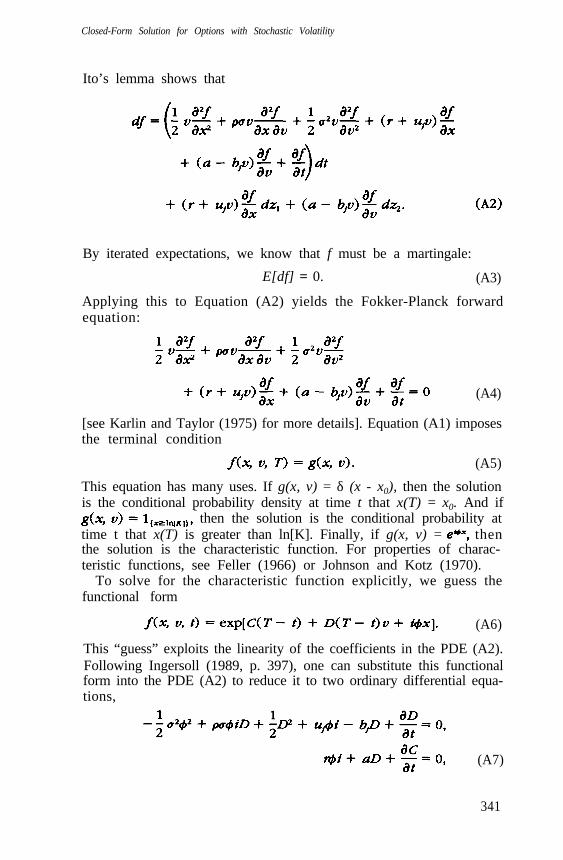
Ito’s lemma shows that

By iterated expectations, we know that f must be a martingale:

E[df] = 0. (A3)

Applying this to Equation (A2) yields the Fokker-Planck forwardequation:

(A4)

[see Karlin and Taylor (1975) for more details]. Equation (A1) imposesthe terminal condition

(A5)

This equation has many uses. If g(x, v) = δ (x - x0), then the solutionis the conditional probability density at time t that x(T) = x0. And if

then the solution is the conditional probability attime t that x(T) is greater than ln[K]. Finally, if g(x, v) = thenthe solution is the characteristic function. For properties of charac-teristic functions, see Feller (1966) or Johnson and Kotz (1970).

To solve for the characteristic function explicitly, we guess thefunctional form

(A6)

This “guess” exploits the linearity of the coefficients in the PDE (A2).Following Ingersoll (1989, p. 397), one can substitute this functionalform into the PDE (A2) to reduce it to two ordinary differential equa-tions,

(A7)

341


subject to

C(0) = 0, D(0) = 0.

These equations can be solved to produce the solution in the text.One can apply the solution technique of this article to other prob-

lems in which the characteristic functions are known. For example,Stein and Stein (1991) specify a stochastic volatility model of the form

(A8)

From Ito’s lemma, the process for the variance is

(A9)

Although Stein and Stein (1991) assume that the volatility process isuncorrelated with the spot asset, one can generalize this to allowz1(t) and z2(t) to have constant correlation. The solution method ofthis article applies directly, except that the characteristic functionstake the form

(A10)

Bates (1992) provides additional applications of the solution tech-nique to mixed jump-diffusion processes.

ReferencesBarone-Adesi, G., and R. E. Whalley, 1987, “Efficient Analytic Approximation of American OptionValues,” Journal of Finance, 42, 301-320.

Bates, D. S., 1992, “Jumps and Stochastic Processes Implicit in PHLX Foreign Currency Options,”working paper, Wharton School, University of Pennsylvania.

Black, F., and M. Scholes, 1972, “The Valuation of Option Contracts and a Test of Market Efficiency,”Journal of Finance, 27, 399-417.

Black, F., and M. Scholes, 1973, “The Valuation of Options and Corporate Liabilities,” Journal ofPolitical Economy, 81,637-654.

Breeden, D. T., 1979. “An Intertemporal Asset Pricing Model with Stochastic Consumption andInvestment Opportunities,” Journal of Financial Economics, 7, 265-296.

Cox, J. C., J. E. Ingersoll, and S. A. Ross, 1985, “A Theory of the Term Structure of Interest Rates,”Econometrica, 53, 385-408.

Cox, J. C.. and S. A. Ross, 1976, “The Valuation of Options for Alternative Stochastic Processes.”Journal of Financial Economics, 3, 145-166.

Eisenberg, L. K.. and R. A. Jarrow, 1991, “Option Pricing with Random Volatilities in CompleteMarkets,” Federal Reserve Bank of Atlanta Working Paper 91-16.

Feller, W., 1966, An Introduction to Probability Theory and Its Applications (Vol. 2). Wiley, NewYork.

342

Closed-Form Solution Options with Stochastic Volatility

Garman, M. B., and S. W. Kohlhagen, 1983, “Foreign Currency Option Values,” Journal of Inter-national Money and Finance, 2, 231-237.

Heston, S. L., 1990, “Testing Continuous Time Models of the Term Structure of Interest Rates.”Ph.D. Dissertation, Carnegie Mellon University Graduate School of Industrial Administration.

Heston, S. L., 1992. “Invisible Parameters in Option Prices,” working paper, Yale School of Organization and Management.

Hull, J. C., 1989, Options, Futures, and Other Derivative Instruments, Prentice-Hall, EnglewoodCliffs, NJ.

Hull, J. C., and A. White, 1987, “The Pricing of Options on Assets with Stochastic Volatilities,”Journal of Finance, 42, 281-300.

Ingersoll, J. E., 1989, Theory of Financial Decision Making, Rowman and Littlefield, Totowa, NJ.

Ingersoll, J. E.. 1990, “Contingent Foreign Exchange Contracts with Stochastic Interest Rates,”working paper, Yale School of Organization and Management.

Jarrow, R., and A. Rudd, 1982, “Approximate Option Valuation for Arbitrary Stochastic Processes,”Journal of Financial Economics, 10, 347-369.

Johnson, N. L.. and S. Kotz, 1970, Continuous Univariate Distributions, Houghton Mifflin, Boston.

Karlin, S., and H. M. Taylor, 1975, A First Course in Stochastic Processes, Academic, New York.

Kendall, M., and A. Stuart, 1977, The Advanced Theory of Statistics (Vol. 1), Macmillan, New York.

Knoch, H. J., 1992, “The Pricing of Foreign Currency Options with Stochastic Volatility,” Ph.D.Dissertation, Yale School of Organization and Management.

Lamoureux, C. G., and W. D. Lastrapes, 1993, “Forecasting Stock-Return Variance: Toward anUnderstanding of Stochastic Implied Volatilities,” Review of Financial Studies, 6, 293-326.

Melino, A., and S. Turnbull, 1990, “The Pricing of Foreign Currency Options with StochasticVolatility,” Journal of Econometrics, 45, 239-265.

Melino, A., and S. Turnbull, 1991, “The Pricing of Foreign Currency Options,” Canadian Journalof Economics, 24, 251-281.

Merton, R. C., 1973, “Theory of Rational Option Pricing,” Bell Journal of Economics and Man-agement Science, 4, 141-183.

Rubinstein, M., 1985, “Nonparametric Tests of Alternative Option Pricing Models Using All ReportedTrades and Quotes on the 30 Most Active CBOE Option Classes from August 23, 1976 throughAugust 31, 1978,” Journal of Finance, 40, 455-480.

Scott, L.O., 1987, “Option Pricing When the Variance Changes Randomly: Theory, Estimation, andan Application,” Journal of Financial and Quantitative Analysis, 22, 419-438.

Stein, E. M., and J. C. Stein, 1991, “Stock Price Distributions with Stochastic Volatility: An AnalyticApproach,” Review of Financial Studies, 4, 727-752.

Wiggins, J. B., 1987, “Option Values under Stochastic Volatilities,” Journal of Financial Economics,19, 351-372.

343

Documents

A Closed-Form Solution for Options with Stochastic