A class of localized solutions of the linear and A class of localized solutions of the linear and nonlinear wave equationsnonlinear wave equations

D. A. Georgieva, L. M. Kovachev

Fourth Conference AMITaNS June 11 - 16, 2012, St. St. Konstantine and Helena, Bulgaria 

2

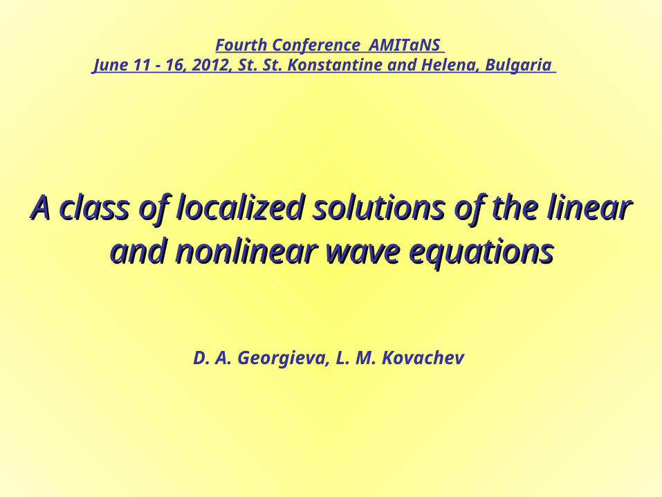
Our aim is to investigate narrow-band and broad-band

laser pulses in femto- and attosecond regions in linear and

nonlinear regime.

AMITaNS, 2012AMITaNS, 2012

3

AMITaNS, 2012AMITaNS, 2012

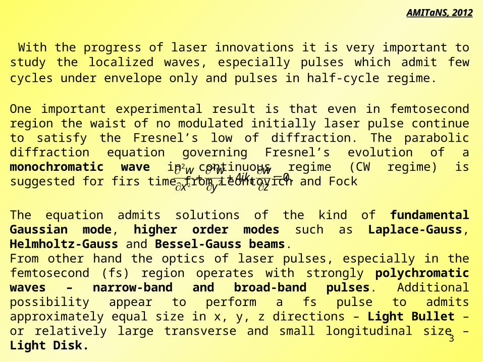
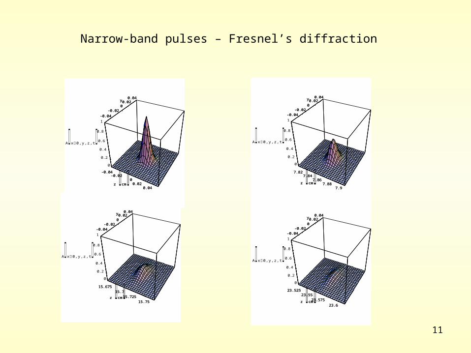
With the progress of laser innovations it is very important to study the localized waves, especially pulses which admit few cycles under envelope only and pulses in half-cycle regime.

One important experimental result is that even in femtosecond region the waist of no modulated initially laser pulse continue to satisfy the Fresnel’s low of diffraction. The parabolic diffraction equation governing Fresnel’s evolution of a monochromatic wave in continuous regime (CW regime) is suggested for firs time from Leontovich and Fock

.04 02

22

2

z

wik

y

w

x

w

The equation admits solutions of the kind of fundamental Gaussian mode, higher order modes such as Laplace-Gauss, Helmholtz-Gauss and Bessel-Gauss beams.From other hand the optics of laser pulses, especially in the femtosecond (fs) region operates with strongly polychromatic waves – narrow-band and broad-band pulses. Additional possibility appear to perform a fs pulse to admits approximately equal size in x, y, z directions – Light Bullet – or relatively large transverse and small longitudinal size – Light Disk.

4

AMITaNS, 2012AMITaNS, 2012

Our work is devoted to obtaining and investigating of analytical solutions of the wave equation governing the evolution of ultra-short laser pulses in air and nonlinear vacuum.

5

AMITaNS, 2012AMITaNS, 2012

The linear Diffraction - Dispersion Equation (DDE) governing the propagation of laser pulses in an approximation up to second order of dispersion for the amplitude function V = V(x,y,z,t ) of the electrical field is

where = k''k0v2 is a number counting the influence of the second order of dispersion, k'' is the group velocity dispersion, k0 is main wave number and v is the group velocity.In dispersionless media it is obtained also the following Diffraction Equation (DE) for the amplitude function A = A(x,y,z,t)

BASIC EQUATIONS

In air 2.110-5 0, and hence DDE is equal to DE, and at hundred diffraction lengths appear only diffraction problems. This means that we can use an approximation 0 and investigate DE only on these distances.

.11

22

2

20 t

A

vA

t

A

vz

Aik

,11

22

2

20 t

V

vV

t

V

vz

Vik

6

AMITaNS, 2012AMITaNS, 2012

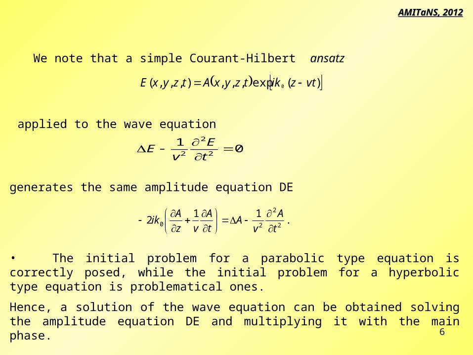
generates the same amplitude equation DE

We note that a simple Courant-Hilbert ansatz

01

2

2

2

t

E

vE

)(exp,,,),,,( 0 vtziktzyxAtzyxE

applied to the wave equation

.11

22

2

20 t

A

vA

t

A

vz

Aik

• The initial problem for a parabolic type equation is correctly posed, while the initial problem for a hyperbolic type equation is problematical ones.

Hence, a solution of the wave equation can be obtained solving the amplitude equation DE and multiplying it with the main phase.

7

AMITaNS, 2012AMITaNS, 2012

FOURIER TRANSFORM

When When 0 0 the fundamental solutions are equal. Therefore we will investigate only the second the fundamental solutions are equal. Therefore we will investigate only the second one.one.

The equations DDE and DE are solved by applying the spatial Fourier transform to the components of the amplitude functions A and V. The fundamental solutions of the Fourier images and  in (kx, ky, kz, t) space are correspondinglyV

tkkkkkkkv

ikkkVtkkkV zzyxzyxzyx 02222

00 211

exp)0,,,(ˆ),,,(ˆ

.exp)0,,,(ˆ),,,(ˆ 20

220

tkkkkkivkkkAtkkkA zyxzyxzyx

and

8

AMITaNS, 2012AMITaNS, 2012

The exact solution of DE can be obtained by applying the backward Fourier transform

tkkkkkivkkkAFA zyxzyx

20

220

1 exp)0,,,(ˆ

Substituting in the latter integral the backward Fourier transform takes the formzz kkk ˆ0

or in details

.exp

exp)0,,,(ˆ2

1 20

2203

zyxzyx

yxzyx

dkdkdkzkykxki

tkkkkkivkkkAA z

.ˆˆexp

ˆexp)0,ˆ,,(ˆexp2

1 222003

zyxzyx

zyxzyx

kddkdkkzykxki

tkkkivtkkkkAvtzikA

9

AMITaNS, 2012AMITaNS, 2012

EXACT SOLUTIONS

An analytical solution of DE is obtained for first time for initial Gaussian light bullet

In this case the 3D backward Fourier transform becomes

I. Gaussian light bullet

.2/exp)0,,,( 20

222 rzyxzyxA

,ˆˆexpˆexp

2

ˆexp

2exp

2

1

02

0222

20

222

0

20

20

3

zyxzyxzyx

zyx

kddkdkkkirzykxkikkkivt

rkkkvtzik

rkA

10

AMITaNS, 2012AMITaNS, 2012

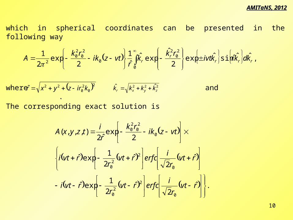
which in spherical coordinates can be presented in the following way

,ˆˆˆsinˆexp2

ˆexpˆ

ˆ1

2exp

2

1 20

2

0

0

20

20

2 rrrr

r kdkrkivtrk

kr

vtzikrk

A

.ˆ2

ˆ2

1expˆ

ˆ2

ˆ2

1expˆ

2exp

ˆ2),,,(

0

2

20

0

2

20

0

20

20

rvtr

ierfcrvt

rrvti

rvtr

ierfcrvt

rrvti

vtzikrk

r

itzyxA

where and . . 2

02

022ˆ kirzyxr 222 ˆˆ

zyxr kkkk

The corresponding exact solution is

11

-0.04-0.02

00.02

0.04z cm

-0.04-0.02

00.02

0.04y

0

0.2

0.4

0.6

0.8

1

Ax 0,y,z,t-0.04

-0.0200.02

0.04z cm

-0.04-0.02

00.02

0.04y

7.827.84

7.867.88

7.9z cm

-0.04-0.02

00.02

0.04y

0

0.2

0.4

0.6

0.8

1

Ax 0,y,z,t7.82

7.847.86

7.887.9

z cm

-0.04-0.02

00.02

0.04y

23.52523.55

23.57523.6

z cm

-0.04-0.02

00.02

0.04y

0

0.2

0.4

0.6

0.8

1

Ax 0,y,z,t23.525

23.5523.575

23.6z cm

-0.04-0.02

00.02

0.04y

15.67515.7

15.72515.75

z cm

-0.04-0.02

00.02

0.04y

0

0.2

0.4

0.6

0.8

1

Ax 0,y,z,t15.675

15.715.725

15.75z cm

-0.04-0.02

00.02

0.04y

Narrow-band pulses – Fresnel’s diffraction

12

-0.04-0.02

00.02

0.04zcm

-0.04-0.02

00.02

0.04y

0

0.2

0.4

0.6

0.8

1

Ax0,y,z,t-0.04

-0.0200.02

0.04zcm

-0.04-0.02

00.02

0.04y

7.827.84

7.867.88

7.9zcm

-0.04-0.02

00.02

0.04y

0

0.2

0.4

0.6

0.8

1

Ax0,y,z,t7.82

7.847.86

7.887.9

zcm

-0.04-0.02

00.02

0.04y

15.67515.7

15.72515.75

zcm

-0.04-0.02

00.02

0.04y

0

0.2

0.4

0.6

0.8

1

Ax0,y,z,t15.675

15.715.725

15.75zcm

-0.04-0.02

00.02

0.04y

23.52523.55

23.57523.6

zcm

-0.04-0.02

00.02

0.04y

0

0.2

0.4

0.6

0.8

1

Ax0,y,z,t23.525

23.5523.575

23.6zcm

-0.04-0.02

00.02

0.04y

31.37531.4

31.42531.45zcm

-0.04-0.02

00.02

0.04y

0

0.2

0.4

0.6

0.8

1

Ax0,y,z,t31.375

31.431.425

31.45zcm

-0.04-0.02

00.02

0.04y

13

0.000050.0001

0.000150.0002

zcm

-0.0001

-0.0000500.00005

0.0001y

0

0.1

0.2

0.3

0.4

Ax0,y,z,t0.00005

0.00010.00015

0.0002zcm

-0.0001

-0.0000500.00005

0.0001y

00.00005

0.00010.00015zcm

-0.0001-0.00005

00.00005

0.0001y

0

0.1

0.2

0.3

0.4

Ax0,y,z,t0

0.000050.0001

0.00015zcm

-0.0001-0.00005

00.00005

0.0001y

-0.0001-0.00005

00.00005

0.0001zcm

-0.0001

-0.0000500.00005

0.0001y

0

0.2

0.4

0.6

0.8

1

Ax0,y,z,t-0.0001

-0.0000500.00005

0.0001zcm

-0.0001

-0.0000500.00005

0.0001y

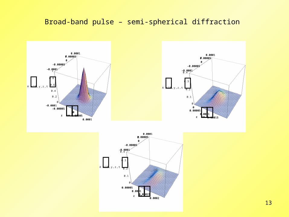
Broad-band pulse – semi-spherical diffraction

14

AMITaNS, 2012AMITaNS, 2012

Multiplying A(x,y,z,t) with the main phase we find an analytical solution of the wave equation

.ˆ2

ˆ2

1expˆ

ˆ2

ˆ2

1expˆ

2exp

ˆ2),,,(

0

2

20

0

2

20

20

20

rvtr

ierfcrvt

rrvti

rvtr

ierfcrvt

rrvti

rk

r

itzyxE

20

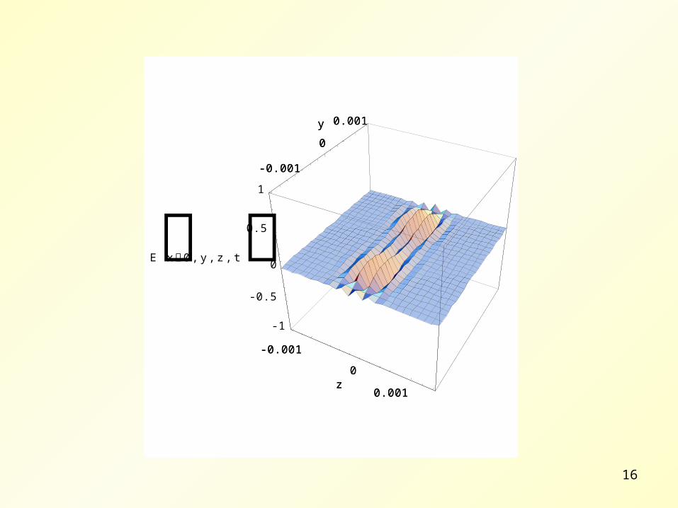
2220 2/exp0,,, rzyxzikzyxE •

• We can observe a translation of the solution in z direction – due to the term exp(ik0z)

• Not stable with time – the amplitude function decreases and the energy distributes over whole space

15

-0.001

0

0.001z

-0.001

0

0.001y

-1

-0.5

0

0.5

1

Ex0,y,z,t-0.001

0

0.001z

-0.001

0

0.001y

-0.001

0

0.001z

-0.001

0

0.001y

-1

-0.5

0

0.5

1

Ex0,y,z,t-0.001

0

0.001z

-0.001

0

0.001y

-0.001

0

0.001z

-0.001

0

0.001y

-1

-0.5

0

0.5

1

Ex0,y,z,t-0.001

0

0.001z

-0.001

0

0.001y

-0.001

0

0.001z

-0.001

0

0.001y

-1

-0.5

0

0.5

1

Ex0,y,z,t-0.001

0

0.001z

-0.001

0

0.001y

-0.001

0

0.001z

-0.001

0

0.001y

-1

-0.5

0

0.5

1

Ex0,y,z,t-0.001

0

0.001z

-0.001

0

0.001y

Fresnel’s type of diffraction as exact solution of the wave equation

16

-0.001

0

0.001z

-0.001

0

0.001y

-1

-0.5

0

0.5

1

Ex0,y,z,t-0.001

0

0.001z

-0.001

0

0.001y

-0.001

0

0.001z

-0.001

0

0.001y

-1

-0.5

0

0.5

1

Ex0,y,z,t-0.001

0

0.001z

-0.001

0

0.001y

-0.001

0

0.001z

-0.001

0

0.001y

-1

-0.5

0

0.5

1

Ex0,y,z,t-0.001

0

0.001z

-0.001

0

0.001y

-0.001

0

0.001z

-0.001

0

0.001y

-1

-0.5

0

0.5

1

Ex0,y,z,t-0.001

0

0.001z

-0.001

0

0.001y

-0.001

0

0.001z

-0.001

0

0.001y

-1

-0.5

0

0.5

1

Ex0,y,z,t-0.001

0

0.001z

-0.001

0

0.001y

-0.001

0

0.001z

-0.001

0

0.001y

-1

-0.5

0

0.5

1

Ex0,y,z,t-0.001

0

0.001z

-0.001

0

0.001y

-0.001

0

0.001z

-0.001

0

0.001y

-1

-0.5

0

0.5

1

Ex0,y,z,t-0.001

0

0.001z

-0.001

0

0.001y

17

AMITaNS, 2012AMITaNS, 2012

Our main purpose is to find exact solutions of the DE and wave equations. Let us consider again the solution of the amplitude function A presented as integral in 3D Fourier space

.ˆˆexp

ˆexp)0,ˆ,,(ˆexp2

1 222003

zyxzyx

zyxzyx

kddkdkkzykxki

tkkkivtkkkkAvtzikA

II. Spherically symmetric finite energy solutions of the wave equation

All terms except the Fourier image of the initial conditions depend on the translated wave number . We can use the Transition theorem to present as a function of only. Let the initial conditions are in form

0,ˆ,,ˆ0kkkkA zyx

zk A

zk

Then, applying the Transition theorem we have

1. The Transition theorem xkgFxixgF exp

.exp0,,,0,,, 0* zikzyxAzyxA

.0,ˆ,,ˆ0,,,ˆ0,,, *0 zyxzyx kkkAkkkkAzyxAF

18

AMITaNS, 2012AMITaNS, 2012

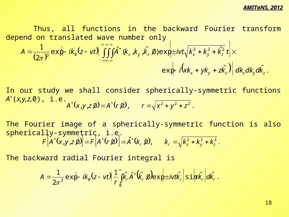
Thus, all functions in the backward Fourier transform depend on translated wave number only

.ˆˆexp

ˆexp)0,ˆ,,(ˆexp2

1 222*03

zyxzyx

zyxzyx

kddkdkkzykxki

tkkkivtkkkAvtzikA

In our study we shall consider spherically-symmetric functions A*(x,y,z,0), i.e.

.,0,0,,, 222** zyxrrAzyxA

The Fourier image of a spherically-symmetric function is also spherically-symmetric, i.e.

.,0,ˆ0,0,,, 222***zyxrr kkkkkArAFzyxAF

The backward radial Fourier integral is

.ˆˆsinˆexp0,ˆˆˆ1exp

2

1 *

0

02 rrrrr kdkrkivtkAkr

vtzikA

19

AMITaNS, 2012AMITaNS, 2012

2. Spherically-symmetric exact solutions with finite energy

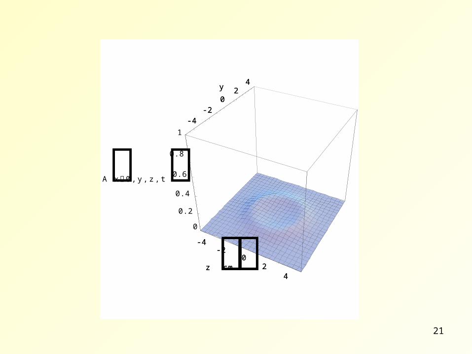
A.A. Localized algebraic function of kind 20

2* /1/1 rrA

20

2

0 1/exp0,,,r

rzikzyxA

*2

0

2

2

02

0

2

2

02

0

2

0

1/10,,,

.1/1,,,

1/exp,,,

Ar

rzyxE

r

ivt

r

rtzyxE

r

ivt

r

rvtziktzyxA

.ˆexpˆ2

0,ˆˆexp2

0,ˆ00

*r

r

rrr

r krk

kAkrk

kA

The Fourier image of the initial data is

Hence, the corresponding solutions of the amplitude and wave equations are

20

-4-2

02

4zcm

-4-2

024y

0

0.2

0.4

0.6

0.8

1

Ax0,y,z,t-4

-20

24

zcm

-4-2

024y

-4-2

02

4zcm

-4-2

024y

0

0.2

0.4

0.6

0.8

1

Ax0,y,z,t-4

-20

24

zcm

-4-2

024y

-4-2

02

4zcm

-4-2

024y

0

0.2

0.4

0.6

0.8

1

Ax0,y,z,t-4

-20

24

zcm

-4-2

024y

-4-2

02

4zcm

-4-2

024y

0

0.2

0.4

0.6

0.8

1

Ax0,y,z,t-4

-20

24

zcm

-4-2

024y

-4-2

02

4zcm

-4-2

024y

0

0.2

0.4

0.6

0.8

1

Ax0,y,z,t-4

-20

24

zcm

-4-2

024y

-4-2

02

4zcm

-4-2

024y

0

0.2

0.4

0.6

0.8

1

Ax0,y,z,t-4

-20

24

zcm

-4-2

024y

21

-4-2

02

4zcm

-4-2

02

4y

0

0.2

0.4

0.6

0.8

1

Ax0,y,z,t-4

-20

24

zcm

-4-2

02

4y

-4-2

02

4zcm

-4-2

02

4y

0

0.2

0.4

0.6

0.8

1

Ax0,y,z,t-4

-20

24

zcm

-4-2

02

4y

-4-2

02

4zcm

-4-2

02

4y

0

0.2

0.4

0.6

0.8

1

Ax0,y,z,t-4

-20

24

zcm

-4-2

02

4y

-4-2

02

4zcm

-4-2

02

4y

0

0.2

0.4

0.6

0.8

1

Ax0,y,z,t-4

-20

24

zcm

-4-2

02

4y

-4-2

02

4zcm

-4-2

02

4y

0

0.2

0.4

0.6

0.8

1

Ax0,y,z,t-4

-20

24

zcm

-4-2

02

4y

-4-2

02

4zcm

-4-2

02

4y

0

0.2

0.4

0.6

0.8

1

Ax0,y,z,t-4

-20

24

zcm

-4-2

02

4y

-4-2

02

4zcm

-4-2

02

4y

0

0.2

0.4

0.6

0.8

1

Ax0,y,z,t-4

-20

24

zcm

-4-2

02

4y

-4-2

02

4zcm

-4-2

02

4y

0

0.2

0.4

0.6

0.8

1

Ax0,y,z,t-4

-20

24

zcm

-4-2

02

4y

-4-2

02

4zcm

-4-2

02

4y

0

0.2

0.4

0.6

0.8

1

Ax0,y,z,t-4

-20

24

zcm

-4-2

02

4y

-4-2

02

4zcm

-4-2

02

4y

0

0.2

0.4

0.6

0.8

1

Ax0,y,z,t-4

-20

24

zcm

-4-2

02

4y

22

AMITaNS, 2012AMITaNS, 2012

B.B. Localized algebraic function of kind 220

2* /1/1 rrA

2

20

2

0 1/exp0,,,r

rzikzyxA

220

2

0

220

2

00

2,,,

2exp,,,

itvrr

itvrtzyxE

itvrr

itvrvtziktzyxA

.ˆexp4

0,ˆˆexp4

0,ˆ0000

*rrrr krrkAkrrkA

The Fourier image of the initial data is

Hence, the corresponding solutions of the amplitude and wave equations are

23

AMITaNS, 2012AMITaNS, 2012

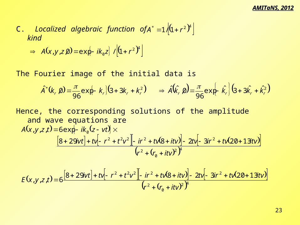
C.C. Localized algebraic function of kind 42* 1/1 rA

420 1/exp0,,, rzikzyxA

42

02

22222

420

2

22222

0

13203282986,,,

1320328298

exp6,,,

itvrr

itvtvirtvitvtvirvtrtvivttzyxE

itvrr

itvtvirtvitvtvirvtrtvivt

vtziktzyxA

22* ˆˆ33ˆexp96

0,ˆˆ33exp96

0,ˆrrrrrrrr kkkkAkkkkA

The Fourier image of the initial data is

Hence, the corresponding solutions of the amplitude and wave equations are

24

AMITaNS, 2012AMITaNS, 2012

D.D. Localized algebraic function of kind 422* 1/1 rrA

4220 1/1exp0,,, rrzikzyxA

44

440

11

32

3,,,

11exp

32

3,,,

irvtirvt

itzyxE

irvtirvtvtzik

itzyxA

.ˆˆexp48

0,ˆˆexp48

0,ˆ 22*rrrrrr kkkAkkkA

The Fourier image of the initial data is

Hence, the corresponding solutions of the amplitude and wave equations are

25

AMITaNS, 2012AMITaNS, 2012

E. Localized algebraic function of kind 322* 1/3 rrrA

3220 1/3exp0,,, rrrzikzyxA

33

330

11

2

1,,,

11exp

2

1,,,

irvtirvtrtzyxE

irvtirvtvtzik

rtzyxA

.ˆˆexp48

0,ˆˆexp4

0,ˆ *rrrrrr kkkAkkkA

The Fourier image of the initial data is

Hence, the corresponding solutions of the amplitude and wave equations are

26

AMITaNS, 2012AMITaNS, 2012

,,01

220

20

32

2

2nkCC

t

C

vC

where γ = 2.

After neglecting two small perturbations terms the corresponding nonlinear amplitude equation for broad-band femtosecond pulses can be reduced to

NONLINEAR PROPAGATION OF BROAD-BAND PULSES IN AIR. LORENTZ TYPE SOLITON.

where γ is the nonlinear coefficient, C0 is the amplitude maximum and n2 is the nonlinear refractive index. The equation admits exact soliton solution propagating in forward direction only

,/~,~1

2~

~lnsec 22222

viatviazyxrrr

rhC

• The 3D+1 soliton solution has Lorentz shape with asymmetric kz spectrum

• The solution preserves its spatial and spectral shape in time

27

299990

300000

300010z

-10

0

10y

0

0.5

1

1.5

2

Ay,z299990

300000

300010z

-10

0

10y

599990

600000

600010z

-10

0

10y

0

0.5

1

1.5

2

Ay,z599990

600000

600010z

-10

0

10y

3.29999 106

3.3 106

3.30001 106z

-10

0

10y

0

0.5

1

1.5

2

Ay,z3.29999 106

3.3 106

3.30001 106z

-10

0

10y

-10

0

10z

-10

0

10y

0

0.5

1

1.5

2

Ay,z-10

0

10z

-10

0

10y

28

-10

0

10z

-10

0

10y

0

0.5

1

1.5

2

Ay,z-10

0

10z

-10

0

10y

299990

300000

300010z

-10

0

10y

0

0.5

1

1.5

2

Ay,z299990

300000

300010z

-10

0

10y

599990

600000

600010z

-10

0

10y

0

0.5

1

1.5

2

Ay,z599990

600000

600010z

-10

0

10y

29

AMITaNS, 2012AMITaNS, 2012

,7245

7 22

74

4

kiikik BBBE

cm

e

AMITaNS, 2012AMITaNS, 2012

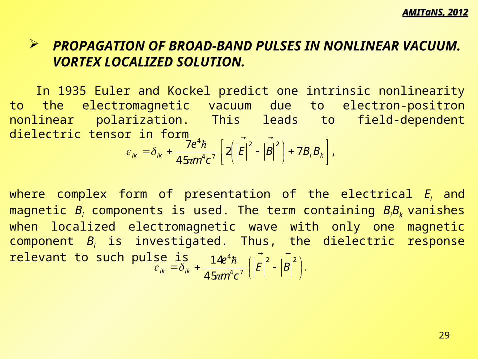
In 1935 Euler and Kockel predict one intrinsic nonlinearity to the electromagnetic vacuum due to electron-positron nonlinear polarization. This leads to field-dependent dielectric tensor in form

PROPAGATION OF BROAD-BAND PULSES IN NONLINEAR VACUUM. VORTEX LOCALIZED SOLUTION.

where complex form of presentation of the electrical Ei and magnetic Bi components is used. The term containing BiBk vanishes when localized electromagnetic wave with only one magnetic component Bl is investigated. Thus, the dielectric response relevant to such pulse is

.45

14 22

74

4

BE

cm

eikik

30

AMITaNS, 2012AMITaNS, 2012

.90

7,0

1

01

74

420

22

2

2

2

22

2

2

2

cm

ekBBE

t

B

cB

EBEt

E

cE

AMITaNS, 2012AMITaNS, 2012

The magnetic field, rather than the electrical filed, appears in the expression for the dielectric response and the nonlinear addition to the intensity profile (effective mass density) of one electromagnetic wave in nonlinear vacuum can be expressed in electromagnetic units as Inl = (|E|2 – |B|2). When the spectral width of one pulse Δkz exceeds the values of the main wave vector Δkz k0 the system of amplitude equations in nonlinear vacuum becomes

We present the components of the electrical and magnetic fields as a vector sum of circular and linear components

.zl

yxc

z

BB

EiEE

E

31

AMITaNS, 2012AMITaNS, 2012

.0

1

01

01

222

2

2

2

222

2

2

2

222

2

2

2

llczl

l

clczc

c

zlczz

z

BBEEt

B

cB

EBEEt

E

cE

EBEEt

E

cE

AMITaNS, 2012AMITaNS, 2012

Hence we get the following scalar system of equations

Let us now parameterize the space-time by pseudo-spherical coordinates (r, τ, θ, φ)

,cossincosh

sinsincosh

coscosh

sinh

rx

ry

rz

rct

where .22222 tczyxr

32

AMITaNS, 2012AMITaNS, 2012

,cosh

1tanh2

131,2222

2

22

2

2

2

2

rrrrrrtc

AMITaNS, 2012AMITaNS, 2012

The d’Alambert operator in pseudo-spherical coordinates is

Where Δθ,φ is the angular part of the usual Laplace operator

),,()()(,,,

,,),,()()(,,,

lll

iii

YTrRrB

cziYTrRrE

which separates the variables. The nonlinear terms appear in radial part only.

,),(),(),(222222

constYTYTYT llcczz

.sin

1sin

sin

12

2

2,

We solve the system of equations using the method of separation of the variables

with an additional constrain on the angular and “spherical“ time parts

33

AMITaNS, 2012AMITaNS, 2012

,,,,03 2

22

2

lcziRRRr

A

r

R

r

R

ri

AMITaNS, 2012AMITaNS, 2012

The radial parts obey the equations

where Ai are separation constants. We look for localized solutions of the kind

.2;1 22 iA

where Ci are another separation constants connected with the angular part of the Laplace operator Yi(θ,φ).

The separation constants Ai, α and γ satisfy the relations

The corresponding τ – dependent parts of the equations are linear

,,,,0coshcoshsinh2cosh 22

22 lcziTAC

d

dT

d

Tdiii

ii

.

lnsec

r

rhR

34

AMITaNS, 2012AMITaNS, 2012

sinh;cosh;cosh lcz TTT

AMITaNS, 2012AMITaNS, 2012

The solutions of the τ – equations which satisfy the constrain condition are

with separation constants for the electrical part Az = Ac = 3; Cz = Cc = 2 and for the magnetic part Al = 3; Cl = 0 correspondingly. The magnetic part of the system of equations do not depend from the angular components, i.e. Yl(θ,φ) = 0, while for the electrical part we have the following linear system of equations

.8;2;42

Using the relation between the separation constants Ai and the real number α we have

The solutions which satisfy the above system and the constrain condition are

.,,2., cziY

Y

i

i

.expsin;cos iTY cz

35

AMITaNS, 2012AMITaNS, 2012AMITaNS, 2012AMITaNS, 2012

Finally we can write the exact localized solution of the system of nonlinear equations representing the propagation of electromagnetic wave in vacuum

The solution can be rewritten in Cartesian coordinates

.sinh

lnsec),,,(

)exp(sincoshlnsec

),,,(

coscoshlnsec

),,,(

2

2

2

r

rhrB

ir

rhrE

r

rhrE

l

c

z

.,1

2),,,(

1

)(2),,,(

1

2),,,(

222224

4

4

tczyxrr

ctrB

r

iyxrE

r

ztzyxE

l

c

z

36

AMITaNS, 2012AMITaNS, 2012AMITaNS, 2012AMITaNS, 2012

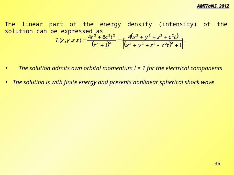
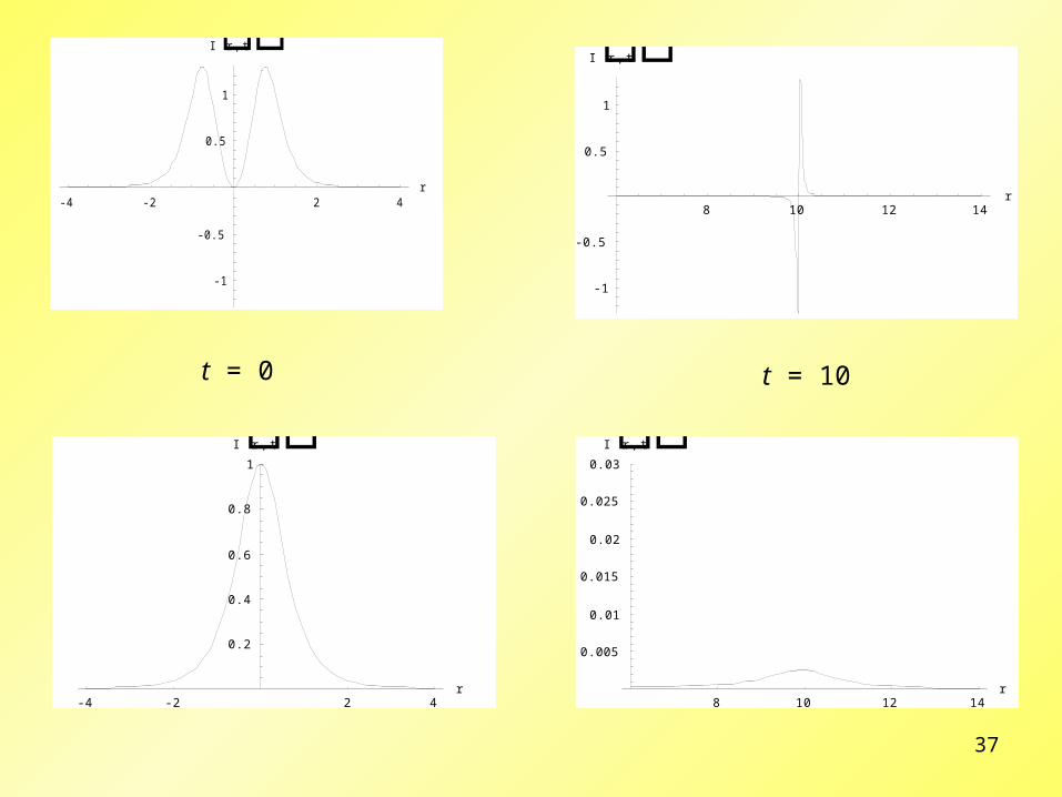
The linear part of the energy density (intensity) of the solution can be expressed as

• The solution admits own orbital momentum l = 1 for the electrical components • The solution is with finite energy and presents nonlinear spherical shock wave

.1

4

1

84),,,(

22222

2222

24

222

tczyx

tczyx

r

tcrtzyxI

37

-4 -2 2 4r

-1

-0.5

0.5

1

Ir,t

8 10 12 14r

-1

-0.5

0.5

1

Ir,t

-4 -2 2 4r

0.2

0.4

0.6

0.8

1Ir,t

8 10 12 14r

0.005

0.01

0.015

0.02

0.025

0.03Ir,t

t = 0 t = 10

38

1) New exact localized solutions of the linear amplitude and wave

equations are presented. The amplitude function decreases and the

energy distributes over whole space for finite time.

2) The soliton solution of the nonlinear wave equation admits

Lorentz’ shape and propagates preserving the initial form and

spectrum.

3) The system of nonlinear vacuum equations is solved in 3D+1

Minkowski time-space. The solution admits own angular momentum

of the electrical part. The solution is with finite energy and presents

nonlinear spherical wave.