Grand Valley State UniversityScholarWorks@GVSU

Masters Theses Graduate Research and Creative Practice

8-2018

A Case Study on Application of Fuzzy Logic basedController for Peak Load Shaving in a TypicalHousehold's Per Day Electricity ConsumptionKrishna P. SharmaGrand Valley State University

Follow this and additional works at: https://scholarworks.gvsu.edu/theses

Part of the Engineering Commons

This Thesis is brought to you for free and open access by the Graduate Research and Creative Practice at ScholarWorks@GVSU. It has been acceptedfor inclusion in Masters Theses by an authorized administrator of ScholarWorks@GVSU. For more information, please contactscholarworks@gvsu.edu.

Recommended CitationSharma, Krishna P., "A Case Study on Application of Fuzzy Logic based Controller for Peak Load Shaving in a Typical Household's PerDay Electricity Consumption" (2018). Masters Theses. 900.https://scholarworks.gvsu.edu/theses/900

1

A Case Study on Application of Fuzzy Logic based Controller for Peak Load Shaving in a Typical Household's Per Day Electricity Consumption

Krishna Prasad Sharma

A Thesis Submitted to the Graduate Faculty of

GRAND VALLEY STATE UNIVERSITY

In

Partial Fulfillment of the Requirements

For the Degree of

Master of Science in Engineering

School of Engineering

August 2018

3

Dedication

To my family.

4

Acknowledgments

I would like to thank Dr. Nicholas Baine, for his guidance and inspiration through the research

process and course-work, for all the emails, meetings, advice, and suggestions. I am grateful to have

Dr. Baine as my Thesis advisor for teaching me research and reminding me to be positive and

encouraged me to continue making progress. I am grateful to all my committee members - Dr.

Heidi Jiao and Dr. Jeffrey Ward for their feedback and constructive criticism to edit the thesis to its

current form. I would like to thank Dr. Shabbir Choudhury for his motivation and guidance. Finally,

I would like to thank Ms. Robin Burris and Ms. Kate Stoetzner for their help throughout my

graduate career. Thank you all for the emails and reminders to helping me stay on top of deadlines.

5

Abstract

The cost of electricity for consumers depends on the cost of generation, transmission, and

distribution of power. The electrical load consumed by consumers per day is not constant

throughout the day. The utilities must be capable of meeting the load demand, which means they

must have enough electricity generation potential and necessary infrastructure. This cost is

significant. However, the revenue they generate will only be for the actual use of electricity by the

consumers. In general, the electrical power generation is done in stages, always generating a base

load. As demand changes throughout the day, additional stages of power generation are brought

online to meet the changes in demand. This approach of management is known as supply-side

management.

Theoretically, if it is possible to manage the load such that there is lower peak demand and the

difference between peak load and base load were minimized, the generation capability and grid

infrastructure required to provide reliable power would be reduced resulting in lower costs for utility

companies and ultimately consumers. This management strategy is referred to as demand-side

management or demand response.

In this research, a small-scale smart grid is modeled in Simulink to mimic the electrical grid. A Smart

controller based on fuzzy logic is developed to control charging and discharging of an electric

vehicle battery to provide extra power during peak times and to act as load (storing energy) during

off-peak time to provide a more manageable and balanced load as seen by the grid. A comparative

study is presented of electricity consumption throughout the day with or without the smart

controller. The results show the significant reduction in peak demand, much smoother load curve

for the grid, and a decrease in per kilowatt cost of electricity for the given day when newer pricing

structures are applied.

6

Table of Contents

Dedication ........................................................................................................................................................... 3

Acknowledgments.............................................................................................................................................. 4

Abstract ............................................................................................................................................................... 5

List of Tables ...................................................................................................................................................... 8

List of Figures ..................................................................................................................................................... 9

Keys to Symbols ............................................................................................................................................... 13

Abbreviations ................................................................................................................................................... 14

Chapter 1 Introduction ................................................................................................................................... 16

1.1 Motivation ........................................................................................................................................ 16

1.2 Purpose ............................................................................................................................................. 35

1.3 Scope ................................................................................................................................................. 35

1.4 Assumptions .................................................................................................................................... 36

1.5 Hypothesis ........................................................................................................................................ 36

Chapter 2 Background .................................................................................................................................... 38

Chapter 3 Methodology .................................................................................................................................. 58

Chapter 4 Results ............................................................................................................................................. 80

Chapter 5 Discussion and Conclusions ..................................................................................................... 103

1.6 Summary ........................................................................................................................................ 103

1.7 Future work ................................................................................................................................... 104

7

Appendix A [48] ............................................................................................................................................ 105

References ...................................................................................................................................................... 110

8

List of Tables

Table 1: US electricity generation by source, amount, and share of the total in 2017 [1] ..................... 17

Table 2: AC/DC Battery Charging Mode description ............................................................................... 52

Table 3: Fuzzy Logic Membership Functions ............................................................................................. 68

Table 4: Rule-Base ........................................................................................................................................... 71

Table 5: Home Energy Management System - Observation table ........................................................... 85

Table 6: Step 2 simulation results .................................................................................................................. 89

Table 7: Yearly cost of Electricity with and without controller for different rate scheme ................ 102

9

List of Figures

Figure 1: Picture representation of electrical power flow from source to consumer [courtesy IER] . 16

Figure 2: Classification of Electrical Transmission Line [Courtesy Circuit Globe] ............................... 19

Figure 3: General Layout of Electricity Network [Courtesy https://commons.wikimedia.org/w/index.php?curid=9676556] ............................................................ 20

Figure 4: Electricity consumption by sector [30] ........................................................................................ 29

Figure 5: Electrical Load classification from utility companies perspective [32] .................................... 30

Figure 6: Load Curve for ISO New England at 10:00 pm [33]................................................................. 31

Figure 7: Household Load Profile [36] ......................................................................................................... 33

Figure 8: Worldwide installed storage capacity for electrical energy [40] ................................................ 39

Figure 9: Comparison of discharge time and power rating for various EES technologies [6] [Courtesy of EPRI] .......................................................................................................................................... 41

Figure 10: Specific Power vs. Specific Energy of different battery types for EES [32] ........................ 41

Figure 11: Application of Inverter and energy storage in storage in grid [34] ....................................... 43

Figure 12: Buck Converter Circuit ................................................................................................................ 44

Figure 13: Boost Converter Circuit ............................................................................................................... 46

Figure 14: Non-inverting two switch buck-boost converter [42] ............................................................. 47

Figure 15: Single phase H-bridge Inverter [43] ........................................................................................... 48

Figure 16: Waveform of Bipolar modulation [43] ....................................................................................... 49

Figure 17: Waveform of Unipolar Modulation [43] .................................................................................... 50

Figure 18: AC-DC battery charging mode [44] ........................................................................................... 51

10

Figure 19: Grid of the Future -Power flow as well as information flow [29] ......................................... 53

Figure 20: Fuzzy Controller Architecture..................................................................................................... 55

Figure 21: Time of use rates for residential consumers [courtesy: data from consumers energy -https://peakpowersavers.com/time/programdetails ] .............................................................................. 57

Figure 22: Steps Involved ............................................................................................................................... 59

Figure 23: Home Energy Management system [courtesy MathWorks® [38] ] ......................................... 61

Figure 24: Control loops in step 1 model ..................................................................................................... 61

Figure 25: Control loops in step 2 model ..................................................................................................... 63

Figure 26: Control Scheme to maintain voltage level ................................................................................. 64

Figure 27: Control Scheme for Battery Current .......................................................................................... 64

Figure 28: shows house 1 data from Pecan Street Project for a whole day. The data provides Solar power generated, Electricity consumed in the day, and the contribution of power form the electric grid. .................................................................................................................................................................... 66

Figure 29: Fuzzy Controller Block Diagram ................................................................................................ 67

Figure 30: Fuzzy Controller Membership Function surface ..................................................................... 68

Figure 31: Input Membership Function 1 plot – P-Error ......................................................................... 69

Figure 32: Input Membership Function 2 plot – SOC............................................................................... 69

Figure 33: Output Membership Function plot – I-Batt (shown for small battery) ................................ 70

Figure 34: Final Simulink Model .................................................................................................................... 72

Figure 35: Inside view of battery block ........................................................................................................ 73

Figure 36: Inside view of moving average calculation block ..................................................................... 74

Figure 37: Inside view of power loss calculation block .............................................................................. 74

11

Figure 38: Inside view of Fuzzy controller block ........................................................................................ 75

Figure 39: Electricity price cents/kWh in the U.S. as of 2013 [courtesy NREL] .................................. 78

Figure 40: Hypothetical cost scenario based on amount of power consumed ....................................... 79

Figure 41: IGBT based DC-AC Inverter model ......................................................................................... 81

Figure 42: Load Profile for Step 1 Simulation ............................................................................................. 82

Figure 43: Power Profile of step 1 simulation showing Battery, Grid, and Solar Power ...................... 83

Figure 44: Voltage and Current at House 1 and Vdc maintained at 370V in step 1 .............................. 84

Figure 45: State of Charge SOC of the battery in step 1 simulation ........................................................ 84

Figure 46: Load Profile of step 2 simulation ............................................................................................... 86

Figure 47: Reference Current for the battery and the State of charge SOC of the battery ................... 87

Figure 48: Voltage and Current at House 1 and Vdc maintained at 370V in step 2 .............................. 88

Figure 49: Power profile of step 2 simulation showing battery, grid, and Solar ..................................... 89

Figure 50: Step 3 simulation power profile - Load and moving average of load ................................... 90

Figure 51: Step 3 simulation – grid and battery power profile for small battery on day 2 .................... 91

Figure 52: Step 3 simulation - State of charge of the small battery on day 2 .......................................... 92

Figure 53: Step 3 simulation – grid and battery power profile for small battery on day 3 .................... 93

Figure 54: Step 3 simulation - State of charge of the small battery on day 3 .......................................... 93

Figure 55: Step 3 simulation – grid and battery power profile for medium battery on day 1 .............. 94

Figure 56: Step 3 simulation - State of charge of the medium battery on day 1 ................................... 95

Figure 57: Step 3 simulation – grid and battery power profile for medium battery on day 2 .............. 96

Figure 58: Step 3 simulation - State of charge of the medium battery on day 2 ..................................... 97

12

Figure 59: Step 3 simulation – grid and battery power profile for big battery on day 1 ....................... 98

Figure 60: Step 3 simulation - State of charge of the big battery on day 1 ............................................ 99

Figure 61: Step 3 simulation – grid and battery power profile for big battery on day 2 .................... 100

Figure 62: Step 3 simulation - State of charge of the big battery on day 2 ......................................... 100

13

Keys to Symbols

η: Combined Efficiency of DC-DC unidirectional converter for Solar to DC Bus, DC-DC bi-

directional converter for battery, and DC-AC bidirectional Inverter for DC bus to Home. This is

assumed to be 95%.

14

Abbreviations

RES : Renewable Energy Sources

IEA : International Energy Agency

EV : Electric Vehicle

EES : Electrical Energy Storage

EPRI : Electric Power Research Institute

ISO : Independent System Operator

RTO : Regional Transmission Organization

DER : Distributed Energy Resources

DG : Distributed Generation

SOC : State of Charge

MPPT : Maximum Power Point Tracking

RER : Renewable Energy Resources

BV : Battery Vehicle

V2G : Vehicle to Grid

PHEV : Plug-in Hybrid Electric Vehicle

GV : Grid Vehicle

BESS : Battery Energy Storage System

PCC : Point of Common Coupling

IPT : Inductive Power Transfer

G2V : Grid to Vehicle

V2H : Vehicle to House

DR : Demand Response

15

HEMS : Home Energy Management System

IGBT : Insulated Gate Bipolar Transistor

IER : Institute for Energy Research

TOU : Time of Use

16

Chapter 1 Introduction

1.1 Motivation

The development of electricity generation, transmission, and distribution is arguably the most

influential of all inventions. It is versatile and converts easily into any form of energy. Traditionally,

the utilization cycle of electrical energy is comprised of three main and separate categories

Generation, Transmission, and Distribution as shown in Figure 1. However, with the development

of renewables, generation is now being performed within the traditional distribution layer. In

addition, there is an emergent third category of storage.

Figure 1: Picture representation of electrical power flow from source to consumer [courtesy IER]

Generation

Table 1 shows the sources of energy and share of total electricity generation in 2017. The traditional

sources of energy are petroleum and nuclear, making up 82.7% of power generation, but each year,

renewables continue to grow and represent a larger percentage of power generation. The most

significant change in renewable sources has been with solar and wind energy.

17

Table 1: US electricity generation by source, amount, and share of the total in 2017 [1]

18

Renewable sources of energy are preferred due to their generation of electricity without the

consumption of fuel and reduced carbon emissions. While they are becoming more cost effective,

they do not produce energy consistently. This lack of consistent generation is one of the main

factors keeping Renewable Energy Sources (RESs) from providing the majority of the world’s

energy needs. According to International Energy Agency, in 2013 renewables accounted for less

than 22% of global electricity generation. Additionally, the share of renewables in overall electricity

generation is expected to rise from over 23% in 2015 to almost 28% in 2021 [2].

Transmission

One of the advantages of electrical energy is the ability to transmit it long distances with relatively

low loss. Transmission of electricity at high voltages allows to move bulk power with low current

and thus low losses. In the US, electricity transmission lines are the high-voltage power lines that

stretch across the entire continent.

Figure 2 shows a categorical representation of transmission system. In the US, there are 240,000

miles long high-voltage lines (230 kV or above) [3]. The large nationwide network of these lines

allows transmission of electricity from the generating power plants to local distribution systems, then

to homes and businesses. The classification of transmission lines depends on many factors; based on

the distance - as Short, Medium, and Long Transmission line.

19

Figure 2: Classification of Electrical Transmission Line [Courtesy Circuit Globe]

Electricity Distribution

As shown in Figure 3, electrical distribution networks are comprised of small voltage lines, which

distribute electricity to individual consumers. The connection shown between the high-voltage

transmission system and the lower-voltage distribution system is performed by distribution

substations with transformers, busbars, and safety circuits such as circuit breakers and disconnects.

Within these substations, transformers lower the transmission voltage to a medium voltage between

2 kV and 35 kV. Then primary distribution lines, connected by distribution feeder system, supply

this medium voltage power to consumers. Additionally, there will be distribution transformers –

usually pole-mounted, located near consumers to lower the medium voltage to the final distribution

voltage level of 480Vac 3-phase, or 120Vac 1-phase.

20

Figure 3: General Layout of Electricity Network [Courtesy https://commons.wikimedia.org/w/index.php?curid=9676556]

21

Smart Grid

Despite the global efforts to reduce consumption of energy and improve efficiency, there is a

growing demand for electrical energy. Much of this is the result of the growing use of electronics

and electric vehicles. This has resulted in significant challenges to meet the need of a growing

demand for energy while trying to move toward a more sustainable and environmentally friendly

energy supply.

The traditional grids are not designed to handle the challenges associated with the changes to power

transmission and distribution that result from more local and distributed forms of power generation,

which are difficult to predict. The result of this shift to renewables is resulting in atypical power

flows. This combined with the congestion that results from the rise in urbanization and access to

electricity to an increasing population, makes it more challenging to provide reliable and secure

power supply, which has become an absolute necessity for modern life due to its use in

transportation, communications, finance, and other critical infrastructures [4]. To address these

challenges a new way of electricity distribution grid system known as Smart Grid is being developed.

According to the U.S. Department of Energy (DoE): Smart Grid generally refers to technologies

that are used to bring utility electricity delivery systems into the 21st century, using computer-based

remote control and automation.

Smart Grid allows reliable and more efficient transmission of electricity. With smart grids, the

restoration of electricity after power disturbances will be much quicker. The communication

platform of Smart Grid will allow utility companies to respond faster to any disturbances in the

system. Congestion management will be improved. Consumers will enjoy lower energy prices as the

cost of operation and management for utility companies will be lower due to improvements in peak

demand management and control. Most importantly, Smart Grids are capable of increased

22

integration of large-scale renewable energy sources as well as smaller customer side source

integration such as EVs and rooftop solar. This allows the grid to move away from traditional

uniderectional operation with all of the supply being provided by large power plants and customers

acting as the demand. Without Smart Grid, the crucial balance between energy supply and demand

would be increasingly difficult to maintain[5].

Much of the change is with residential buildings becoming smarter with extensive use of smart

appliances, integration of information and communication technology, and in-house power

generation using renewable energy resources (RER) [6]. Inconsistent and uncontrolled local load

demand and generation at this individual consumer level adds up to significant amount when the

number of consumers grow. In this project, an attempt to curb the irregular peaks and troughs in

the load at individual consumer level is attempted by developing a Fuzzy based smart controller

capable of shaving peaks and providing a smoother load graph utilizing an EV as energy storage

unit, which can store or consume electrical energy as required to maintain a consistent demand for

the grid.

The peak load is what dictates the required generation and distribution capacity of a power system.

If a system cannot meet the demanded load, some of the load will not be supplied through the

process of load shedding; this is also known as a brown out. Therefore, systems are required to be

overbuilt to meet this peak load and are underutilized most of the time. A decrease in the difference

between the average load and the peak load would result in a significant decrease of the wasted

capacity in the system and improve efficiency

In addition, end users are becoming more aware of the energy resource they use and see advantages

in the sustainable operation of the energy system [7]. Consumers are now monitoring their energy

use to minimize their cost. The adjustable and controllable loads provide ways to gauge the optimal

23

amount of energy required to fulfil all of their demands in a sustainable manner[8], scheduling run

times of smart appliances at times of low demand on the grid [9] costs comparatively less to

consumers and is a good motivator to achieve sustainable operation of the energy system. On the

other hand, the utility companies are investing in carbon-free generation of energy, through the use

of renewable resources[10][11][12]. In an effort to reduce peak demand and improve efficiency,

consumers can obtain a significant price reduction through demand response programs

[13][5][14][15], allowing flexibility in the schedule of electricity consumption to more evenly

distribute load throughout the day.

Distributed Generation

Distributed generation (DG) is defined as electric power generation within distribution networks, on

the customer side of the network. Distributed generation can be discussed based on different

aspects. Ackerman et al [16] tried to define DG based on purpose, location, rating of distributed

generation, the power delivery area, the technology, the environmental impact, the mode of

operation, the ownership, and the penetration of distributed generation.

It is expected that DG will play an increasing role in electric power systems in the near future. One

of the most attractive benefits of DG is the possibility of improving the continuity of power supply.

DG plants can be designed to supply portions of the distribution grid in the event of an upstream

supply outage[17].

Distributed generation can also benefit the electric utility by decreasing overcrowding on the grid,

reducing the need for new generation and transmission capacity, and offering supplementary

services such as voltage support and demand response. With advancements in power electronics and

control technologies, the large-scale effective integration of a range of distributed generation and

24

energy storage technologies into the existing electric power infrastructure may finally become

possible and economically feasible.

Due to their growing popularity, electric vehicles are a growing user of electricity but also represent

significant energy storage when connected to a charging station. The concept of using the EVs as a

distributed resource – load and generation/storage device – by their integration into the grid is

known as vehicle-to-grid (V2G)[18].

The idea is to integrate the aggregated electric vehicles into the grid as distributed energy resources.

These vehicles will act as controllable loads and sources. During off-peak conditions, the system will

maintain the load level by acting as additional load. During peak demand, it will provide energy to

the grid, acting as a backup power source and providing additional capacity.[18]

The V2G concept falls into a category of devices called Battery Energy Storage Systems (BESS),

consisting of batteries and an inverter/charger, are an option for this next-generation distributed

energy storage and are particularly well suited to buildings and communities due to their safe, silent,

scalable, zero/low-maintenance, and efficient operation that does not depend upon topography,

geology, or moving parts [19]. BESS achieves a smooth power transition from 100[%] of power

injection to 100[%] of power absorption without adversely affecting the voltage at the Point of

Common Coupling (PCC) or the current at the DC side.[20]

Research on using Electric Vehicles as a BESS has gained popularity recently. EVs equipped with

large batteries are capable of directly charging or discharging to the grid; consequently, they are the

most desirable and sustainable form of energy storage to be used.

V2G strategies have been found to have a negative impact on the cell performance, possibly

diminishing the lifetime of battery packs to less than 5 years. In contrast, delayed Grid-to-Vehicle

25

(G2V) strategies were found to have a negligible effect on cell performance at room temperature,

though these strategies could be advantageous in warmer climates.[21]

EVs could discharge during the daily peak loads, replacing the peak capacity generators that are only

used during peak demand hours. If these vehicles want to discharge during the peak hours, they will

have to charge during the off-peak hours. In this case, the energy which is stored during off-peak

hours, is released during peak hours to relieve congestion in the grid infrastructure, supplying peak

power and providing load leveling at the same time. Supplying peak power is possibly difficult for

EVs because of the relatively long-duration and the storage limitations. Thus, supplying peak power

is generally not profitable as the largest cost is the wear of the batteries. Load leveling is desireable.

The total consumption of electricity will not be lowered but shifted to the hours of low electricity

consumption which are the off-peak hours to minimize the power losses and to increase grid

efficiency. The implementation of smart meters or real-time pricing and coordinated charging is

essential for consumers to be incentivized to participate.[22]

The use of EVs to perform load levelling does not guarantee a significant reduction in cost and

emissions; however, the use of EVs in presence of renewable energy resources will help with cost

and emission reduction. The best approach would be to utilize RERs and EVs together to minimize

the amount of energy that needs to pass over transmission lines. Unfortunately, there is a

considerable up-front cost for RERs development that must be taken into consideration [23].

Another popular approach rather than V2G could be Vehicle to Home (V2H). In single households

the V2H can essentially perform similar load levelling at the home level to smooth the individual

load curves, which in turn adds up to have a similar effect in larger scale as a V2G would. Haines et

al [24] have concluded that Vehicle-to-home avoids the infrastructure and tariff problems associated

with vehicle-to-grid. Their research shows that V2H used to control peak demands at household

26

levels for short duration of time incurred by running high power consuming appliances provides the

ability of managing individual peak demand at the household level. The collective result will provide

smoother demand from the grid, providing utilities companies a more manageable load. The

flexibility to shift or feed peak demand in the home using energy storage allows the electric load seen

by the grid to remain more constant throughout the day. This would allow more efficient and cost

effective electricity generation to be used. Vehicle-to-home would improve the effectiveness of

renewable energy sources; excess generation can be stored and used when generation is low.

Vehicle-to-grid (V2G) allows connection of multiple cars and houses to the grid. In contrast,

vehicle-to-home is more limited; a single vehicle is used to supply a single house. The trade-off is

simplicity versus flexibility; more vehicles working together offer flexible storage but will be more

difficult to control [24]. Both V2G and V2H are a form of distributed storage (acting as either

source or load) and they are located at the distribution end of the grid. Therefore, the power

transmission line requirement is minimal compared to traditional centralized generation and thus the

costs of transmission infrastructure and transmission losses are reduced. Consequently, V2H

represents the simplest case with regards to infrastructure and transmission. A single house

operating V2H will have simple infrastructure requirements and negligible transmission losses.

Importance of renewable energy

For EVs, the core objective is to be able to utilize the battery in those vehicles to serve as source of

energy for transportation while driving. A secondary objective is to utilize the battery in the EV as

an electrical load and supply that charges itself during off-peak time and discharges during peak

time. Integrating such a battery energy storage system (BESS) with a solar photovoltaic (PV) system

or a wind farm can make these intermittent renewable energy sources more dispatchable [25]

27

In an effort to incentivize customers to participate, allowing their vehicles to be used as distributed

grid storage, electricity prices could vary hourly [26]. This would enable customers to use their

vehicle to store energy during low-cost (off-peak times) and use that energy during peak times. This

could also be used to improve the value of customer owned renewable energy resources.

Additionally, real-time price-based distributed resource management applications can be embedded

into smart meters and automatically executed on-line for determining the optimal operation of

residential appliances while considering uncertainties in real-time electricity prices. This will enable

consumers to handle financial risks brought by dynamic real-time price uncertainty, and individual

consumers can make their own choices based on their preferences on computational time, cost

minimization, and risk aversion [27].

Due to the increasing competition in liberalized electricity markets with involvement of many

Independent System Operators (ISOs) and Regional Transmission Organizers (RTOs), a successful

customer retention as well as a cost-efficient allocation of electric energy becomes more and more

important. Therefore, new innovative strategies are sought, which promise on the one hand a long-

term customer retention and assure, on the other hand, a more cost-efficient provision of electric

energy. [28]

Distributed generation can be either inertial synchronous generators or non-inertial converter

interfaced. The latter of which can come online or go offline in plug-and-play fashion. The

combination of different generation sources with different methods of operation makes the

microgrid control a challenging task, especially when the microgrid operates in an autonomous

mode. The DGs that have variable frequency sources (wind), high frequency sources (microturbine)

and direct energy conversion sources (PV) are connected to a micro grid via power electronics

interfaces [29]. As energy needs change, pricing will change. For example, distributed generating

28

capacity will come online to take advantage of price increases; however, each of the different types

of generators take a different amount of time to come online. The resultant lag between stimulus

and reaction by different systems will make it increasingly difficult to control the system as

independent distributed generation makes up a larger percentage of the grid’s capacity.

Energy Consumption and Management

The three major sectors of electricity consumption are Commercial, Industrial, and Residential, with

residential consuming almost one-third of total energy used. Figure 4 shows energy consumption by

each sector along with the share of individual applications in each sector. The electricity

consumption rate in each sector is growing day-by-day. The demand for electricity in these sectors in

any given day varies. With variation in energy demands the supply must also be capable of adapting

accordingly as the supply and demand must match up at all times. The industrial sector sees a larger

demand during the day time while the residential sector has the highest demand in the evenings.

Furthermore, the share of electrical demand also varies depending upon the development level of

individual countries. Industrialized nations have electricity consumption similar to what is shown in

Figure 4. In comparison, the residential sector’s share is dominant in underdeveloped countries. At

the industrial level, the trend of electricity usage is fairly consistent. However, for commercial and

residential sectors the demands in usage of electricity varies based on many environmental factors

such as seasons, unusual day (e.g. extremely hot or cold), and special occasions (sports events,

celebration day - religious or non-religious)

29

Figure 4: Electricity consumption by sector [30]

To move away from fuel based generation, a cost-effective large scale energy storage system is

necessary for the utilities to maintain load and supply balance, providing an uninterrupted power

supply. The most successful method is a pumped hydro system but its use is limited by the lack of

water resources at suitable geographical locations to build cost-effective storage. Furthermore, the

battery technology we have now gets exponentially expensive with the increase in the amount of

storage. Unfortunately, at present there is no universal technology that can store electrical energy

30

cost-effectively on a large scale [31]. For that reason, balancing authorities rely on generators to

respond to changes in demand at a moment’s notice.

Figure 5 shows different categories of loads from the perspective of utility companies in a given day.

Baseload is the load of electricity demand guaranteed to exist throughout the day. Peak load occurs

for a limited span of time in the day. This span of time varies for industrial, commercial, and

residential loads as mentioned earlier. Figure 6 shows a typical Load Curve for ISO New England

and the share of fuel for generation. Utility companies forecast load, usually, a day ahead to ensure

the best utilization of resources and to ensure uninterrupted supply. As previously mentioned, the

future goal is to store energy during low-peak hours and then use that stored energy to meet the

excess demand during peak hours.

Figure 5: Electrical Load classification from utility companies perspective [32]

31

Figure 6: Load Curve for ISO New England at 10:00 pm [33]

Supply Side Control

Rather than simply having centralized power generation at a few large fossil fuel or nuclear power

plants, more non-traditional distributed energy resources are being added to the grid every day.

Integration or interconnection of distributed energy resources is evolving as an emerging power

scenario for electric power generation, transmission and distribution infrastructure globally. The

reasons for this are the scarcity of fossil fuel in future, widespread deployment of advanced

Distributed Energy Resources (DERs) technologies, and deregulation of electric utility industries. In

addition to that, the public’s ever growing awareness of environmental impact of traditional electric

power generation is a crucial factor. These issues are changing the power generation concept

worldwide and opening up new challenges in the generation and distribution markets. Small non-

conventional generation combined with Distributed Generation (DG) is rapidly becoming attractive

because it produces electrical power with less environmental impacts, easy to install, and highly

efficient with increased reliability. As the awareness on environmental issues like global warming is

increasing, renewable energy sources are becoming more significant sources of energy in modern

power scenario. Geographical, environmental, political and financial factors of different countries

32

are also leading to the increased use of renewable energy resources, which include wind–electric

conversion systems, photovoltaic systems, and biomass resources.

The low power generation capacity of DER has motivated the need for integration of different types

of DERs and loads in the form of microgrid to enhance the power generation capacity, reliability

and marketability of dispersed type of microsources with a promising approach to reduce the load

congestion on the conventional power system or utility grid and facilitating localized generation at

the customer end. The effective integration of DERs depends on the versatile nature of DGs such

as photovoltaic system, wind power, small hydro turbines, tidal, Combined Heat Power (CHP)

based microturbines, biogas, geothermal, fuel cells including battery storage facilities etc. that have

the potential to support conventional power system with many issues involved with their

interconnections. In this perspective, IEEE P1547- 2003 is a benchmark model for interconnecting

DERs with Conventional Electric Power System [1] which provides guidelines to general

interconnection requirements (e.g. response to abnormal conditions including operation, power

quality, and safety conditions including operation in utility grid connected and islanded mode) [34].

Load Side Control

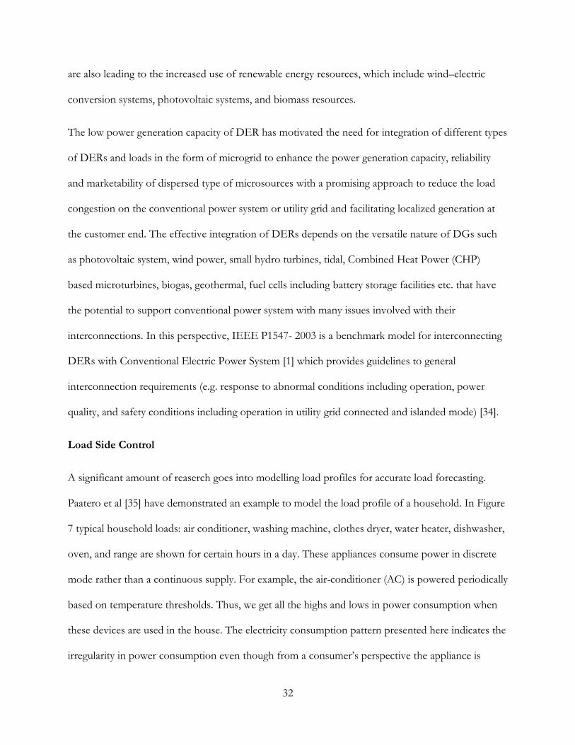
A significant amount of reaserch goes into modelling load profiles for accurate load forecasting.

Paatero et al [35] have demonstrated an example to model the load profile of a household. In Figure

7 typical household loads: air conditioner, washing machine, clothes dryer, water heater, dishwasher,

oven, and range are shown for certain hours in a day. These appliances consume power in discrete

mode rather than a continuous supply. For example, the air-conditioner (AC) is powered periodically

based on temperature thresholds. Thus, we get all the highs and lows in power consumption when

these devices are used in the house. The electricity consumption pattern presented here indicates the

irregularity in power consumption even though from a consumer’s perspective the appliance is

33

turned on all the time. If the usage of household loads was random, then the loads of multiple

households would average together to a constant load with no variation. Unfortunately, the usage of

household loads is heavily correlated among homes and result in a significantly high difference

between base and peak power consumption. Also, in any neighborhood it cannot be guaranteed that

all the houses will have modern electrical appliances. With the rising popularity of EVs the energy

consumption pattern will also change as the EVs will likely consume electricity at night time whereas

traditionally this was not the case. This increased irregularity in power consumption indicates that

battery-based backup system with very fast response is necessary to have a controlled and smooth

load curve as seen by the supply grid when these household loads are active.

Figure 7: Household Load Profile [36]

34

At the individual household level load management scheme could be implemented to manage the

timing of use of home appliances to shift the peak load and have a smoother load demand

throughout the day. Research is currently being done to develop an algorithm that schedules

thermostatically controlled household loads based on price and consumption forecasts which

consider users’ comfort settings to meet an optimization objective such as minimum payment or

maximum comfort. The formulation of an appliance commitment problem is described using an

electrical water heater load as an example [37]. Furthermore, the scheduling could be done based on

the price per kWh of electrical energy, which varies throughout the day. Currently, utility size

electricity providers are required to provide quotes for day-ahead delivery of electricity and submit

their quote for all hours in the next day simultaneously. The price often varies between same hour of

two different days, althouth the overall trend throughout a day period tend to remain more or less

the same [26].

Shifting the load by scheduling the usage of smart appliance is an effective method, but it is limited

by what a customer desires for comfort and convenience. Beyond this additional capability would be

needed in the form of energy storage through the use of batteries in an EV or through an alternative

product that is installed in the home. Such products were introduced by Tesla in 2015 namely their

Powerwall and Powerpack. Both units utilize rechargeable lithium-ion batteries to provide stationary

energy storage. The Powerwall was designed for a variety of residential scale applications, which

include solar self-consumption, time of use load shifting, backup power, and off-the-grid use. The

larger Powerpack was designed for commercial or electric utility grid use for a variety of purposes,

which include peak shaving, load shifting, backup power, demand response, microgrids, renewable

power integration, frequency regulation, and voltage control.

35

1.2 Purpose

The purpose of this research is to develope a basic Simulink model capable of representing small

scale electricity distribution network to feed an average household, analyze the electric load curve for

a 24 hour period, and design a fuzzy logic based controller that will help reduce the peak electricity

consumption from the grid by charging and discharging a battery system. The goal of this battery

system is to supply energy to the house during higher demand time and charge the battery during

lower demand time. The controller strategy will be to maintain the demand on the electrical grid

near the average for a 24-hour period. Different scenarios of battery configuration and control

schemes are tested. Finally, percentage reduction in peak load, and economical analysis from the

reduction in peak demand is performed.

1.3 Scope

The scope of this thesis is the development of a fuzzy logic controller for a home battery storage

system. This was evaluated using a simulation that characterized the effect on the cost of energy.

A representative model of small scale electrical distribution network was designed in two stages in

Simulink. First model based on modification to Home Energy Management System [38] where in a

typical house, available energy sources are solar panels, battery storage, and the external power grid.

The second stage of modelling involved a simplified model in Simulink to observe power transfer

and control using a fuzzy logic controller. The control of voltage and current in an actual microgrid

are simulated in the first stage separately from a long-term simulation of energy flow which is done

in second stage. This was done to accommodate limited computational resources. Based on design

rules of the controller the battery was capable of charging or discharging with respect to two input

variables: difference in Power and State of Charge (SOC)of Battery. The necessary load data with

36

solar power data was obtained from Pecan Street Inc. Microgrid Research [39]. The peak power

consumption before and after the introduction of controller and the battery is observed. The

information acquired is then used to analyze reduction in peak power consumption and an

economic analysis for the reduction in cost of distribution ensued by less peak load is performed.

1.4 Assumptions

Assumptions in the analysis are

Power grid is capable of supplying all the load requirements as well as absorbing the solar

power when no load is present.

Battery model does not take into account the temperature and ageing effects.

First model’s ability to maintain voltage level and successful imitation of actual microgrid

scenario holds true with analysis using final model - only concerned with the power.

Solar Power is extracted at maximum power point. The reference model already contains an

MPPT based solar supply. Further development of MPPT controller is out of the scope of

this research.

Droop characteristics; decrease in frequency of the system with increase in load and increase

in frequency when active power is injected holds true in the models.

1.5 Hypothesis

This study examines how a fuzzy based controller applied to a small scale microgrid feeding an

average household reduces peak load of the grid relative to the moving average power of grid. It is

expected that the utilization of battery storage will result in a more constant load on the grid,

reducing the peak load. It is expected that depending upon battery capacity (Ah) and SOC of the

battery for same consumer load, the utilization of battery changes the Load Curve and provide

37

overall less power consumption from the grid to reduce the cost of distribution for the power

companies which in return leads to decrease in cost of per kW electricity for the consumers.

Furthermore, a hypothetical pricing scheme with charges based on amount of energy consumed is

tested with expectation that the change in Load curve due to load shifting will result in lower cost of

energy.

38

Chapter 2 Background

Electricity Storage System and Schemes

Currently, there are a variety of energy storage technologies available for large-scale applications

which include mechanical, electrical, chemical, and electrochemical systems. Based on capacity,

existing energy storage is dominated by pumped hydroelectric; however, there is the recognition that

battery systems can offer some high-value opportunities, provided that the costs can be lower than

existing pumped storage.

Energy storage system at grid level and household level have different characteristics. The grid-based

storage system must have the capability of storing a large amount of energy whereas by comparison

household storage is much smaller. Also, the most efficient energy storage options tend to be more

expensive and at very large scale the cost could be astronomical. An example would be highly

efficient Li-on batteries used at household level are encouraged by the proliferation of EVs, whereas

less efficient but cheaper Sodium-Sulphur batteries are preferred at the transmission and distribution

levels in the grid.

Batteries have the advantage of a faster response time compared to the traditional pumped hydro

storage plants. Peak shaving and load shifting can be accomplished with long response times.

However, short response times are required to help regulate frequency, to allow load following, and

to allow load levelling at a fast and precise manner, which would lead to improvements in grid

reliability, stability, and cost compare to pumped hydro at grid scale. However, pumped hydro is still

dominate at the grid level as mentioned earlier due to the enormous cost associated with batteries,

but this is changing every day with the growing popularity of distributed generation facilitated by the

smart grid. Pumped hydro is scheduled to run prior to the starting of peak load, which is forecasted

39

to achieve the goal of uninterrupted supply even during peak times. Alternatively, at the household

level faster batteries could respond to any abrupt changes in load behavior without the need of

forecasting. For this thesis, research is focused on a single household utilizing a Li-ion battery

system.

Figure 8 provides an overview of worldwide installed storage capacity for electrical energy. Pumped

hydro comprises 99% of total electrical energy storage. These numbers will change in the future as

more electric cars and UPS systems at household level increase in the future. The advantage of

Smart Grid is to be able to tap in and store the energy from a variety of small energy generators

spread out throughout the grid compared to traditional remote and big power plants.

Figure 8: Worldwide installed storage capacity for electrical energy [40]

Energy storage systems based on Li-ion batteries are expected to take a different route than either

Na/S or redox-flow batteries. The development of Li-ion batteries for commercial electronics and

automotive applications enabled this technology to address reliability, cycle life, safety, and other

40

factors that are equally as important for stationary energy storage. The well-established research

environment for developing new low-cost materials, and recent efforts directed at low-temperature

processing and renewable organic electrodes provide the basis for future advances in the field.

Furthermore, in the future electric vehicles will rise in demand as evident by the recent success of

Tesla Motors. The rise in demand will provide incentives to the manufactures to produce EVs at a

large scale. With the rise in production, the improvements in manufacturing processes will follow,

leading to the production of EVs and EV related technologies like Li-ion batteries at substantial

economic scale that will in return lower the costs required to make Li-ion battery technology viable

for BESS. Thus enabling the possibility of using batteries previously used in the automotive

industries and electric vehicles connected to home power system to serve as power storage devices

for vehicles in large-scale energy storage applications [32].

Figure 9 shows the power rating and corresponding discharge time for various energy storage

devices. These batteries are suitable for less than 10 MW power rating and unlike pumped hydro

these are incapable of providing discharge at the high-power rating for hours. Among the batteries,

Li-ion batteries have higher specific power and specific energy with respect to their weight, as shown

in Figure 10. The capability to store more energy in smaller foot print allows to exploit the energy

storage potential of Li-ion batteries at much larger scale. Modern cell-phones and most small

electrical or electronic devices exclusively use Li-ion batteries. Li-ion batteries are getting more

popular in larger energy storage requirement devices as well. Recent examples being electric vehicles.

Due to aforementioned advantages of Li-ion batteries, their universal presence and growing

popularity, smaller footprint in addition to the fact that the individual cells can be connected in

series and parallel in numerous ways to virtually achieve any level of operational voltage make Li-ion

batteries the best choice of battery used in this research.

41

Figure 9: Comparison of discharge time and power rating for various EES technologies [6] [Courtesy of EPRI]

Figure 10: Specific Power vs. Specific Energy of different battery types for EES [32]

42

Inverter based microgrid

Inverters can be used in DGs in a microgrid system. These inverter based DGs have fast switching

operation compared to traditional rotational machine based DGs with large inertia. Interconnecting

parallel inverters provide fast response and smooth transfer of energy from grid connected mode to

islanded mode and vice versa. During the mode transfer, to avoid large transient, it is important to

have inverter based DGs operating in parallel mode [34].This property of parallelly operated inverter

based DGs provide solution for diversity in DER generation and uncertainty in use of renewable

energy resources.

Figure 11 shows a typical Inverter based DG system connected to the utility grid. Here, the utility

grid is providing supply to a step-down transformer and into the Intelligent Bypass Switch (IBS) and

Point of Common Coupling (PCC). The critical and non-critical loads can be supplied by different

supply lines. These lines connect to inverters connected to the storage systems and DERs

43

Figure 11: Application of Inverter and energy storage in storage in grid [34]

Subramanyam et al [41] used Bi-directional AC-DC converter for various combinations of power

generated by a PV panel and available grid power. The SOC of battery and load demand were used

to decide whether to link the solar system and/or the battery to the grid. The inverter’s ability to

44

respond fast and less overall loss in the power electronics involved make them highly desirable

entities in DGs with generating sources found near to the consumers.

DC-DC Converter

Converters are useful to change voltage level of DC supply to higher or lower voltage level. The

converters that reduce the voltage level are called buck converters (see Figure 12). The converters

used to increase the voltage level are called boost converters (see Figure 13 ). Both Buck and Boost

Converters can operate in either Continuous Current Mode (CCM) or Discontinuous Current Mode

(DCM) – If the current through the inductor never falls to zero during the cycle it is CCM or else

DCM, at the exact zero point it is critical mode.

Figure 12: Buck Converter Circuit

When the switch labeled “S” is closed in Figure 12, the voltage across the inductor is given by,

VL = VI − Vo (1)

45

The current through the inductor rises linearly (in approximation, so long as the voltage drop is

almost constant). As the diode is reverse-biased by the voltage source V, no current flows through it.

When the switch is opened in Figure 12, the diode is forward biased. The voltage across the inductor

is given by,

VL = −Vo (2)

And the current decreases. When

𝑡ON = DT (3)

And,

𝑡OFF = (1 − D)T (4)

The output voltage is

(VI − VO)DT − VO (1 − D) T = 0 (5)

Vo = DVI (6)

From this equation, it can be seen that the output voltage of the converter varies linearly with the

duty cycle for a given input voltage. As the duty cycle 𝐷 is equal to the ratio between 𝑡𝑂𝑁 and the

46

period T, it cannot be more than 1. Therefore, Vo ≤ VI, This is why this converter is referred to as

step-down converter.

In case of Boost converter, When the switch S is closed in Figure 13, the current across the inductor

is increased. When the switch S is open, the energy is transferred into the capacitor as the only path

offered to inductor current is through the fly-back diode D, the capacitor C and the load R.

The output voltage is

(VIDT + (VI − VO) (1 − D) T = 0 (7)

Vo =1

1 − DVI (8)

Above equations shows that the output voltage is always higher than the input voltage (as the duty

cycle goes from 0 to 1), and that it increases with D, theoretically to infinity as D approaches 1. This

is why this converter is sometimes referred to as a step-up converter.

Figure 13: Boost Converter Circuit

47

Non-inverting two switch Bi-directional DC-DC Converter [42]

A noninverting step-down converter can be obtained by cascading the buck and boost converters.

The output filter capacitor of the buck converter can be removed and the buck output filter inductor

and the boost input filter inductor can be combined to obtain a noninverting buck-boost converter

as shown in Figure 14

Figure 14: Non-inverting two switch buck-boost converter [42]

Bi-directional DC-AC Inverter

A grid-tie inverter converts direct current (DC) into an alternating current (AC) suitable for injecting

into an electrical power grid. The inverter must be capable of bidirectional power transfer. The DC-

AC inversion could be based on unipolar or bipolar Pulse width Modulation (PWM) technique.

Figure 15 shows a typical single-phase h-bridge inverter.

48

Figure 15: Single phase H-bridge Inverter [43]

The upper and the lower switches in the same inverter leg work in a complementary manner with

one switch turned on and other turned off. Thus, we need to consider only two independent gating

signals Vg1 and Vg3 which are generated by comparing sinusoidal modulating wave Vm and triangular

carrier wave Vcr. The inverter terminal voltages are obtained denoted by VAN and VBN and the

inverter output voltage VAB = VAN-VBN. Since the waveform of VAB switches between positive and

negative dc voltages this scheme is called bipolar PWM. The waveforms of bipolar modulation are

shown in Figure 16.

49

Figure 16: Waveform of Bipolar modulation [43]

The unipolar modulation normally requires two sinusoidal modulating waves Vm and Vm- which are

of same magnitude and frequency but 180° out of phase. The two modulating wave are compared

with a common triangular carrier wave Vcr generating two gating signals Vg1 and Vg3 for the upper

two switches S1 and S3. It can be observed that the upper two devices do not switch simultaneously,

which is distinguished from the bipolar PWM where all the four devices are switched at the same

time. The inverter output voltage switches between either between zero and +Vd during positive half

cycle or between zero and –Vd during negative half cycle of the fundamental frequency thus this

50

scheme is called unipolar modulation. The waveform of unipolar modulation are shown in Figure

17.

Figure 17: Waveform of Unipolar Modulation [43]

Figure 18 shows an AC/DC battery charging topology. The battery can be charged by the grid

power supply. Here, in the boost operation for AC/DC battery-charging mode, unipolar modulation

is selected to control the single-phase converter. The stages of operation is shown in

51

Table 2.

Figure 18: AC-DC battery charging mode [44]

52

Table 2: AC/DC Battery Charging Mode description

AC/DC Battery Charging Mode

Figure 18 Switch & Diode

Active Inductor

Charge by Capacitor

Charged by Battery

Charged by

a S2 & S3 Grid & Capacitor - Capacitor

b S2 & D4 Grid - Capacitor

c D1 & D4 - Grid & Inductor Grid & Inductor

d S1 & S4 Capacitor - Capacitor

e S1 & D3 - - Capacitor

f D2 & D3 - Grid & Inductor Inductor

Peripherals of Modern Grid

It is clear that the future of electricity generation is leaning towards renewable energy sources

coupled with energy storage systems and manageable loads. Instead of producing as much is

required, managing the load and integrating smaller and flexible sources to get optimum return will

be the new norm in the power industry. Figure 19 provides a brief glimpse of future grids. Here we

can see the two types of networks – electrical and information, working simultaneously to provide

reliable electricity. The distribution of power starts from the substation through a feeder breaker

then a capacitor controller is used to optimize voltage and improve power factor. After that a

regulator controller is installed. These voltage regulators are used to maintain voltage in the system

along with additional regulator controllers to attenuate harmonics. The voltage level is then stepped

down using transformers from where the electricity is supplied to the meters at the consumer.

At the user level, Energy Management Systems (EMS) can connected to the meter to manage the

secondary source of power, smart appliances and energy storage in response to the user’s energy

demand. The EMS would be able to receive information from the smart meter and manage power

consumption at consumer level. Communication signals or control signal via the information

53

network would also be received at the breaker, capacitor controller, transformer and smart meter.

Instructions are received primarily on two basis – Asset Management and Billing and Accounting.

The Asset management instructions are processed by different frameworks for gathering, managing,

and analyzing data such as Global Information System (GIS) and Supervisory Control and Data

Acquisition (SCADA). This thesis develops a fuzzy-logic based EMS.

Figure 19: Grid of the Future -Power flow as well as information flow [29]

54

Fuzzy Logic in Controls [45]

A controller is developed to control the flow of energy in the system. It is possible to either charge

or discharge the battery, but a controller needs to be developed to decide how much and when. The

battery needs to be utilized in such a way that it reults in meaningful load shaving off of the grid and

at the same time must be able to charge itself when the load on grid is significantly low. The main

objective is to have the grid supply the demand as consistently throughout the day as possible. To

achieve this goal, the power required by a home is to be held close to the average (4kW in house1)

throughout the day. It is clear that the control scheme is not a binary scheme of whether the battery

should supply or consume power in order to balance the grid. The control scheme must take into

account both the criteria for the battery to charge or discharge as well as by how much. Not only is

the load a factor, but the SOC (state of charge) of the battery is one as well. While it is clear that a

fully charged battery cannot be charged any more nor a fully discharged battery can provide more

energy. An ideal controller would never encounter either state. Fuzzy logic based controllers are

most suitable for this kind of control scenario. Compared to traditional control schemes where the

behavior and function of the model must be precise, fuzzy controllers provide ability to use human

expertise and experiences directly to the control scheme. However, while designing fuzzy controllers

for any given system, the system must be observable and controllable. Fuzzy controllers provide

flexibility in design where knowing a “good enough” solution for control purpose is sufficient.

Fuzzy control provides a formal methodology for representing, manipulating, and implementing a

human’s heuristic knowledge about how to control a system.

In this thesis, a typical multiple input single output (MISO) Mamdani Fuzzy Controller is designed.

The inputs and outputs are defined in fuzzy sets through membership functions. The membership

functions also define the range of the inputs and outputs. Careful consideration of the range is

55

important to avoid saturating either the input or output of the controller. The fuzzy controller block

diagram in Figure 20 shows a fuzzy controller embedded in a closed-loop control system. The plant

outputs are denoted by y(t), its inputs are denoted by u(t), and the reference input to the fuzzy

controller is denoted by r(t).

Figure 20: Fuzzy Controller Architecture

The fuzzy controller has four main components:

1. The “rule-base” holds the knowledge, in the form of a set of rules, of how best to

control the system.

2. The inference mechanism evaluates which control rules are relevant at the current time

and then decides what the input to the plant should be. The process utilizes Membership

Functions, Logical Operations, and If-Then Rules. There are number of different

membership functions expressed in various shapes such as Triangular, Gaussian and

Trapezoidal.

56

3. The fuzzification interface simply modifies the inputs so that they can be interpreted and

compared to the rules in the rule-base. The function of the fuzzy inference is to produce

an output fuzzy set from the defined rules.

4. The defuzzification interface converts the conclusions reached by the inference

mechanism into the inputs to the plant. There are many different de-fuzzifiers, but this

work uses the most popular centroid method. This method gives the centroid of the area

under the output fuzzy set.

Essentially, one should view the fuzzy controller as an artificial decision maker that operates in a

closed-loop system in real time. It gathers plant output data y(t), compares it to the reference input

r(t), and then decides what the plant input u(t) should be used to ensure that the performance

objectives will be met.

Cost of Electricity for Consumers

Electricity pricing varies a lot for different types of consumers, household consumers are charged a

higher tariff compared to industrial consumers. Industries consume more power at higher voltages,

which results in a lower current for the same amount of power, leading to a more efficient and less

lossy supply. Furthermore, utility companies offer time-based rate programs to encourage

consumers to shift their usage during off peak times, reducing the peak. The more likely consumer is

to increase the peak load, the expensive the cost of electricity. Figure 21 shows a typical household

time of use rate, it is clear that during the peak time the cost of electricity is also high, discouraging

usage at that time and allowing for additional revenue to offset the additional costs associated with

electricity generation at peak times.

57

Figure 21: Time of use rates for residential consumers [courtesy: data from consumers energy -https://peakpowersavers.com/time/programdetails ]

0

2

4

6

8

10

12

14

16

18

¢/kW

h

Time of day in Hours

Time of Use Rates (¢/kWh)

58

Chapter 3 Methodology

As previously mentioned, the traditional sources of energy for the generation of electrical power will

have smaller share of total generation in the future. Smarter grids with demand side management

having distributed generation made possible by renewable sources of energy will prevail. Load-side

management will have a significant impact on the next generation of electrical energy distribution.

More use of V2G or V2H concepts utilizing EVs, BESS, and other similar systems with load

levelling or load shifting functionality along with RESs will reduce the burden of primary generators

to fulfill varying electrical demand.

This research does not attempt to explain all new generation, transmission, distribution, or control

schemes associated with the smart grid of the future. The research is focused on observing the

application of a battery system in the home. Here, an attempt is made to model a small household

electricity supply grid containing Solar as an RES, a battery system, and a load profile of a typical

household. Then a Fuzzy-based controller is designed to manage the energy in the system, choosing

to charge or discharge the battery based on the SOC of the battery and the variation in power pulled

in from the grid. The idea is to maintain the grid at a moving average of power in the given day such

that, the previous spikes in load curve, which are present with the absence of controller, are now

lesser in magnitude and overall load profile is much smoother due to the application of the fuzzy

based control scheme. Additionally, the research tries to analyze the change in peak demand

quantitively and as a consequence the change in the cost of electricity for the consumer.

In this work, the application of battery at the users end, to provide a more manageable, somewhat

consistent, and econimical load profile for any given house, is demonstrated by the modelling of the

home electric distribution grid. The flow chart in Figure 22 provides the progression of this research

project.

59

Figure 22: Steps Involved

Step 1

Any microgrid model representing a RES, Battery, and Grid supplying to Load must have certain

electrical characteristics. The high-voltage DC (HVDC) bus needs to be maintained at a constant

voltage and the home electrical system need to have its voltage and frequency controlled. The

injection of power from the RES or Battery into the HVDC bus can easily effect its voltage. The

DC-DC converter connected to the solar power system is designed to achieve MPPT and will adjust

in voltage and current to maximize the power generated. The DC-DC converter for the battery is

bidirectional and will be controlled to maintain a desired energy flow into or out of the battery.

60

Neither of these converters can be used to control the voltage of the HVDC bus due to their

primary control goals of maximizing solar power generation and battery energy flow respectively.

Therefore, the bidirectional DC-AC inverter must be used to control the voltage of the HVDC bus.

With the primary control goal of the DC-AC inverter to maintain a constant voltage on the HVDC

bus, the flow of energy will change direction as needed. For example if there is little solar power and

the battery is commanded to charge, the draw on the HVDC bus will increase resulting in a

tendancy for the voltage to sag, but the AC-DC inverter would fight that tendancy by allowing

energy to flow from into the bus. On the other hand, if there was abundent solar energy being

generated, the energy flow into the HVDC bus would result in a tendancy for the voltage to rise and

the inverter would react by transfering energy to the home. Additionally, it is assumed that the grid

is capable of supplying as well as absorbing power and will do so to maintain the voltage level of the

home electrical system. MathWorks® in the Fall of 2017 released a Home Energy Management

System model (as shown in

Figure 23) publicly in their website with similar concept. It is available in MATLAB version R2017b

or later as power HEMS [38].

61

Figure 23: Home Energy Management system [courtesy MathWorks® [38] ]

As mentioned above, the model satisfies some of the requirements and is suitable to use as a

reference model. In this research, we need the battery, solar, and the grid connection present all the

time and simulate for 24 hours.

Figure 24: Control loops in step 1 model

62

Step 2

The above model has significant limitations. The most notable of which was that the solar and

battery were not designed to work with the grid. The model assums that either the grid or the solar

battery system are used to power the home. This makes the model fairly simple and easier to

control. To allow for the use of all energy sources simultaneously as well as the ability to charge the

battery from the grid, the above reference model was considered a starting point and has been

modified significantly.

The resulting model was simulated in a variety of cases demonstrating the change in energy flow

when the battery is charging versus discharging. In the new model, the battery is controlled by

providing reference value for the current varying from +10A to -10A for the PID loop in the

Battery Controller section. Due to high computational requirements, the simulation is limited to 6

seconds, which is adequate to demonstrate the controller works. The simulation results prove that

the aforementioned control strategy and system is stable and works.

The desired results must have the following characteristics.

• Constant voltage level on the HVDC bus.

• Solar operating in MPPT mode.

• Model capable of reflecting anticipated results i.e. lower power provided by the grid

to the system while the battery is discharging.

• Load matching effects of the battery while it is charging.

63

Figure 25: Control loops in step 2 model

Figure 26 shows a block diagram of the control loop used to regulate the High Voltage Bus at 370V

regardless of the amount of power injected or drawn out. The flow of energy from the solar and to

the battery are treated as disturbances, which the controller is designed to reject. The controller

input is the difference between the voltage of the HVDC bus and the reference value of 370V. The

controller output is the PWM signal pulses, which drive the transistors in the bi-directional inverter.

It is also worthy of note that the inverter also matches the frequency and phase of the AC side of

the inverter to that of the grid.

64

Figure 26: Control Scheme to maintain voltage level

Figure 27 shows the current control scheme to draw or supply a certain amount of current to the

battery. In this case, the control loop is designed to control the current into or out of the battery.

The controller measures the difference in the measured current relative to the commanded current

and outputs PWM pulses to the DC-DC converter between the battery and HVDC bus.

There is a third control loop that performs MPPT for the solar system, that was left unmodified

from the original simulation and is outside the scope of this thesis.

Figure 27: Control Scheme for Battery Current

65

Step 3

The model in step 2 established that it is possible to develop the electronics to control the flow of

energy in and out of battery system tied to both a solar system and the grid at a residential home.

Due to the computational requirements, the previous model is not practical for simulating an energy

management system for an entire day. Instead a second model is developed to simulate only the flow

of energy over the period of a day or longer, showing the behavior of the fuzzy based energy

management system.

Step 3-A

For a 24 hour simulation, a typical household load data is taken from Pecan Street’s microgrid

research [39]. The data include Power generated by Solar, Power consumed by the customer and net

Power in the grid. This data is for 1st of September in 2011. As shown below, PHouse is the actual

electricity consumed, PSolar during the day helped so supply during the day time and hence dip in the

contribution of grid. In this thesis, moving forward it is assumed that the Solar will contribute as is

and the power from Grid after the solar has already contributed is the load for step 3 onward

simulations. The individual electrical loads are not specified from the original researchers.

66

Figure 28: shows house 1 data from Pecan Street Project for a whole day. The data provides Solar power generated, Electricity consumed in the day, and the contribution of power form the electric grid.

𝑃𝐻𝑜𝑢𝑠𝑒 − 𝑃𝑆𝑜𝑙𝑎𝑟 = 𝑃𝐺𝑟𝑖𝑑 (9)

67

Step 3-B

A fuzzy based controller is developed to control the flow of energy in the system. Following

paragraphs summarizes the different components of fuzzy controller development mentioned in

background section. Figure 29 shows the fuzzy control block representation.

Figure 29: Fuzzy Controller Block Diagram

Controller design consists the following components. Here, Membership functions are trapezoidal at

extreme values of range and triangular in between. The trapezoidal shape ensures that the extreme

vaules are default values if/when the data is out of range, Furthermore, the triangular membership

functions within the range of input ensures 100% total at all possible values. This way a continuous

and smooth surface is obtained meaning there is no discontinuity to disrupt operation (see Figure

30).

68

Figure 30: Fuzzy Controller Membership Function surface

Table 3: Fuzzy Logic Membership Functions

Input Member 1

First input is the difference between power in the grid and the moving average of power. The five

triangular membership functions are N-HIGH, N-SMALL, ZERO, P-SMALL and P-HIGH ; N in

the name stands for Negative and P for Positive. For example, the region for P-SMALL is when the

difference between power in grid and moving average power is between positive 0 to 2000, watts

(see Figure 31 ). See Table 3 for further information.

N-HIGH -ve 2500 to -ve 1000; Trapezoidal mf EMPTY 0 to 25; Triangular mf HD High Discharge

N-SMALL -ve 2500 to 0; Triangular mf LOW 0 to 50; Triangular mf LD Low Discharge

ZERO -ve 1000 to 1000; Triangular mf HALF 25 to 75; Triangular mf NONE No Charging/Discharging

P-SMALL 0 to 2000; Triangular mf OK 50 to 100; Triangular mf LC Low Charge

P-HIGH 1000 to 2000; Trapezoidal mf HIGH 75 to 100; Triangular mf HC High Charge

Input Member 1 P-error (Watts) Input Member 2 SOC (%) Output Member I-output (Amps)

69

Figure 31: Input Membership Function 1 plot – P-Error

(The membership function for P-HIGH is highlighted in red)

Input Member 2

Second input is categorization of SOC of the battery. There are five triangular membership

functions in this input – EMPTY, LOW, HALF, OK, and HIGH. For example, OK represents

when SOC is between 50-100% (see Figure 32 ). See Table 3 for further information.

Figure 32: Input Membership Function 2 plot – SOC

(The membership function for EMPTY is highlighted in red)

Mem

ber

ship

Power (W)

Mem

ber

ship

SOC (%)

70

Output Member

The output of the fuzzy controller is the amount of current to be supplied for charging the battery

or current drawn from the battery during peak times. Negative current to the battery represents

discharge of the battery and positive current to the battery represents charging of the battery. The

triangular output membership functions are HD, LD, NONE, LC, and HC (see Figure 33 ). See

Table 3 for further information.

Figure 33: Output Membership Function plot – I-Batt (shown for small battery)

(The membership function for High Discharge [HD] is highlighted in red)

Fuzzy Rules

Based on the input membership functions mentioned earlier, their conditional combinations

provides a rule base for the fuzzy system to decide the amount of current to be supplied or drawn

from the battery to obtain a smoother load curve that follows the moving load average as closely as

possible eliminating peaks in the load curve. Table 4 provides a self explanatory review of the rules

used in this case study.

Mem

ber

ship

Output Current (A)

71

Table 4: Rule-Base

Rule # Conditions Outcome

1 If (P-Error is N-HIGH) and (SOC is EMPTY) then (I-Batt is HC)

2 If (P-Error is N-HIGH) and (SOC is LOW) then (I-Batt is HC)

3 If (P-Error is N-HIGH) and (SOC is HALF) then (I-Batt is HC)

4 If (P-Error is N-HIGH) and (SOC is OK) then (I-Batt is LC)

5 If (P-Error is N-HIGH) and (SOC is HIGH) then (I-Batt is NONE)

6 If (P-Error is N-SMALL) and (SOC is EMPTY) then (I-Batt is HC)

7 If (P-Error is N-SMALL) and (SOC is LOW) then (I-Batt is HC)

8 If (P-Error is N-SMALL) and (SOC is HALF) then (I-Batt is LC)

9 If (P-Error is N-SMALL) and (SOC is OK) then (I-Batt is LC)

10 If (P-Error is N-SMALL) and (SOC is HIGH) then (I-Batt is NONE)

11 If (P-Error is ZERO) and (SOC is EMPTY) then (I-Batt is HC)

12 If (P-Error is ZERO) and (SOC is LOW) then (I-Batt is HC)

13 If (P-Error is ZERO) and (SOC is HALF) then (I-Batt is LC)

14 If (P-Error is ZERO) and (SOC is OK) then (I-Batt is NONE)

15 If (P-Error is ZERO) and (SOC is HIGH) then (I-Batt is LD)

16 If (P-Error is P-SMALL) and (SOC is EMPTY) then (I-Batt is NONE)

17 If (P-Error is P-SMALL) and (SOC is LOW) then (I-Batt is LD)

18 If (P-Error is P-SMALL) and (SOC is HALF) then (I-Batt is LD)

19 If (P-Error is P-SMALL) and (SOC is OK) then (I-Batt is HD)

20 If (P-Error is P-SMALL) and (SOC is HIGH) then (I-Batt is HD)

21 If (P-Error is P-HIGH) and (SOC is EMPTY) then (I-Batt is NONE)

22 If (P-Error is P-HIGH) and (SOC is LOW) then (I-Batt is LD)

23 If (P-Error is P-HIGH) and (SOC is HALF) then (I-Batt is HD)

24 If (P-Error is P-HIGH) and (SOC is OK) then (I-Batt is HD)

25 If (P-Error is P-HIGH) and (SOC is HIGH) then (I-Batt is HD)

Here, the numerical value of Output membership function differs based on the size of the battery

used, this is discussed in details in Step 4. E.g. -12.5 to 12.5 Amps for a small battery (24.5Ah).

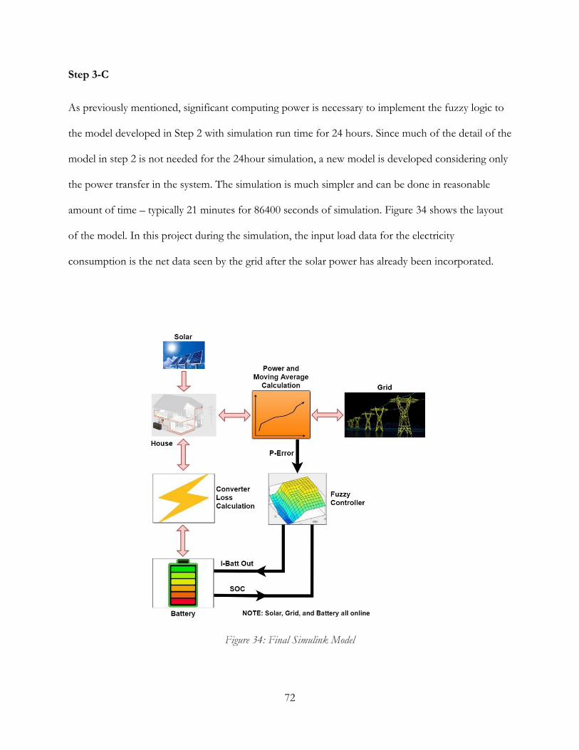
72

Step 3-C

As previously mentioned, significant computing power is necessary to implement the fuzzy logic to

the model developed in Step 2 with simulation run time for 24 hours. Since much of the detail of the

model in step 2 is not needed for the 24hour simulation, a new model is developed considering only

the power transfer in the system. The simulation is much simpler and can be done in reasonable

amount of time – typically 21 minutes for 86400 seconds of simulation. Figure 34 shows the layout

of the model. In this project during the simulation, the input load data for the electricity

consumption is the net data seen by the grid after the solar power has already been incorporated.

Figure 34: Final Simulink Model

73

Figure 35 provides an inside look of the battery block of the model. A generic battery model

available in MATLAB is used as the battery and was configured with the characteristics of a Li-ion

battery. A current source I-batt is the output of the fuzzy controller. Depending upon the polarity of

this current supply the battery is considered to be either charging or discharging. For instance, -10 of

I-batt means the battery is discharging 10 amps, which is 2000 watts of power as the chosen battery

here is of 200V.

Figure 35: Inside view of battery block

Figure 36 shows the moving average calculation block. The moving average is the value to which we

want the grid to maintain its power.

74

Figure 36: Inside view of moving average calculation block

Figure 37 is the inside view of power loss calculation block. PdcBatt is the actual power from the

battery, this block represents efficiency loss of power from DC to AC conversion and standby

power losses in the electronics involved as well.

Figure 37: Inside view of power loss calculation block

Figure 38 shows the inside of the fuzzy controller block in the model. P_error and SOC are the two

input parameters fed to the fuzzy controller and an output Ibatt is obtained.

75

Figure 38: Inside view of Fuzzy controller block

In this model, calculations based on equations (10) and (11) provide system losses.

𝑃𝐴𝐶 = 𝑃𝐷𝐶 − 𝑃𝐿𝑂𝑆𝑆 (10)

𝑤ℎ𝑒𝑟𝑒, 𝑃𝐿𝑂𝑆𝑆 = 𝑃𝑆𝑇𝐵𝑌 + 𝑃𝐷𝐶*(1-η) (11)

η is the efficiency of the DC-DC converter. PDC is the power supplied by the battery, PSTBY is the

standby power loss of the converter and inverter system.

Furthermore, calculation of the moving average power is as shown in

𝑃𝑀𝑜𝑣𝐴𝑣𝑔(𝑡=0)= (0.0001 ∗ 𝑃𝐿𝑂𝐴𝐷) + (0.9999 ∗ 4000) (12)

𝑃𝑀𝑜𝑣𝐴𝑣𝑔(𝑡)= (0.0001 ∗ 𝑃𝐿𝑂𝐴𝐷) + (0.9999 ∗ 𝑃𝑀𝑜𝑣𝐴𝑣𝑔(𝑡−1)

) (13)

76

Step 4

The simulation runs for 86400 seconds and results are obtained for PGRID and PBATTERY according to

PLOAD , and SOC of the battery. The reduction in PGRID due to application of the energy management

system and battery is measured from the output graphs.

The data from house1 is used to run the model in three different cases

Case 1: Small Size Battery

Case 2: Medium Sized Battery

Case 3: Large Size Battery

It is also desirable that the battery users not extract more than 70%–80% of the available capacity at

any time as recommended by McEvoy et al [46].

In the aforementioned cases following criteria are used to analyze the battery and grid performance

House 1 has a total of 98 kWh total power consumption from grid ( Load demand – Solar

supply). In each case this same amount of energy consumption is used.

Battery sizing:

Case 1: A small battery (with a nominal voltage of 200V) is defined as the battery capable of

supplying 5% of the daily total 98 kWh energy in 2 hours. In this case, the controller will be

capable of charging or discharging maximum current 0.5*(Ah rating of the battery) per hour.

Therefore, the small battery will have the capacity to supply 4.9 kWh at 200 V in 2 hours.

The chosen battery will have 24.5 Ah and the controller will prompt the battery for

maximum charge or discharge current of 12.25A.

Case 2: A medium battery is defined as the battery capable of supplying 20% of the total 98

kWh of energy at 200V in 2 hours. In this case, the controller will be capable of a charging

77

or discharging maximum current of 0.5*(Ah rating of the battery) per hour . Therefore, the

medium battery will have the capacity to supply 19.6 kWh at 200 V in 2 hours. The chosen

battery will be 98 Ah and the controller will prompt the battery for maximum charge or

discharge current of 49A.

Case 3: A large battery is defined as the battery capable of supplying 50% of the total 98

kWh of energy at 200V in 2 hours. In this case, the controller will be capable of a charging

or discharging maximum current of 0.5*(Ah rating of the battery) per hour. Therefore, the

large battery will have capacity of supplying 49 kWh at 200 V in 2 hours. The chosen battery

will be 245 Ah and the controller will prompt the battery for maximum charge or discharge

current of 122.5A.

Economic Analysis

The cost of electricity for consumers is charged based on per unit electricity consumed, where per

unit electricity is 1 kWh (i.e. electricity consumption of 1 kW for 1 hour). Typically, a US household

consumes 903 kWh per month. The cost of electricity is 12.23 cents/kWh (US national average –

residential customers) [47]. This brings the average total to $110.44 per month. In this work, the

electricity used from the grid in kWh is calculated, then after using fuzzy based controller to reduce

the load from the grid during peak times by shifting the load appropriately. The cost of electricity

within the day itself varies depending on season, time of the day, sector of customer – residential, or

industrial, or commercial.

78

Figure 39: Electricity price cents/kWh in the U.S. as of 2013 [courtesy NREL]

The actual Time of Use based rate discussed in the introduction section in Figure 21 provides the

TOU to be used as Rate in Equation (14) to calculate the average daily cost of electricity

consumption.

𝐴𝑣𝑒𝑟𝑎𝑔𝑒 𝐷𝑎𝑖𝑙𝑦 𝐶𝑜𝑠𝑡 𝑜𝑓 𝐸𝑙𝑒𝑐𝑡𝑟𝑖𝑐𝑖𝑡𝑦 = 𝑅𝑎𝑡𝑒 ∗ 𝐷𝑎𝑖𝑙𝑦 𝑘𝑊ℎ (14)

79

Furthermore, a different cost of electricity scenario based on amount of power consumed and not

the time based is provided in Figure 40. The Rate is defined as 8₵/kWh up to 2kW power

consumption. The rate is double - 16₵/kWh for 10kW energy consumption.

Figure 40: Hypothetical cost scenario based on amount of power consumed

0

2

4

6

8

10

12

14

16

18

0 0.5 1 1.5 2 2.5 3 3.5 4 4.5 5 5.5 6 6.5 7 7.5 8 8.5 9 9.5 10

¢/kW

h

kW

Hypothetical cost scenario - Energy Consumption based price of electricity

80

Chapter 4 Results

Step 1 Simulation

The Home Energy Management System Simulink model results are shown in Figure 43 and Figure

45. In this simulation, a solar panel with an MPPT controller generates 5kW for the entire duration

of simulation – 6 secs. The electric grid is capable of providing or absorbing any surplus power in

the system. The grid is connected to the home for the first 2 seconds of the simulation and the

battery system is isolated from the home. From 2 to 4 seconds into the simulation the grid is

disconnected and the home is powered by the battery and solar system. During the last 2 seconds of

the simulation, the grid is reconnected and the battery is isolated from the home.

Throughout the simulation, the voltage level is maintained at 370 Vdc in the HVDC bus, meaning

that any power injection in the system is done with a maintained voltage level on the bus. Figure 41

shows a typical IGBT based DC-AC bidirectional inverter configuration. IGBT1 and IGBT4 allows

one way of current flow whereas IGBT2 and IGBT3 allows the flow of current in opposite polarity.

81

Figure 41: IGBT based DC-AC Inverter model

Figure 42 shows the two loads – Load 1 of 3kW and Load 2 of 3kW and their activation times. Load

1 is connected from the start of simulation until 0.5 seconds, then both Load 1 and Load 2 are

connected from 0.5 seconds to 1 seconds. Load 1 and Load 2 are removed between 1.5 seconds to 2

seconds. The battery is connected at 2 seconds. At 2.5 seconds Load 1 is active again and at 3

seconds Load 2 is also active. Both loads are disconnected at 3.5 seconds and reconnected back at 4

seconds, when the battery is taken offline and grid is now online.

82

Figure 42: Load Profile for Step 1 Simulation

Figure 43 shows that the battery is responding to the load demand in absence of the Grid. Here, the

grid power is positive when the grid is supplying the power and battery power is negative when it is

discharging to provide power in absence of the grid. The solar is continuously providing 5kW. It

should be noted that there is a significant power spike during the switching between the grid and

HVDC power system. This is undesirable and is addressed by the modifications in the next step.

83

Figure 43: Power Profile of step 1 simulation showing Battery, Grid, and Solar Power

In the step 1 simulation, the Grid (AC side) is bidirectional. It performs absorption/power supply

from/to HEMS as a voltage source. Figure 44 shows V-Grid is constant from 0 to 2 secs, then 4 to

6 secs when the Grid is online. The load demand that cannot be fulfilled by the solar power is

supplied by the grid when the grid is online. The changes in I-Grid can be seen during 0.5 to 1 secs

when Load 1 is turned on and then 1 to 1.5 secs when both the loads are turned on. Additionally,

during 2 to 4 secs when the grid is offline I-Grid is 0 and during 0 to 0.5, 1.5 to 2, and 4 to 6 secs

when the loads are not turned on, the voltage and current level are stable. Meanwhile, Battery (dc) is

also bidirectional operation. It performs absorption/supply of power from/to HEMS as current

source. As shown in Figure 44, there are changes in voltage (AC) level at the house during 2 to 4

secs, at this time Grid is offline and battery is supplying power addition to power being supplied by

the solar system.

84

Figure 44: Voltage and Current at House 1 and Vdc maintained at 370V in step 1

Figure 45: State of Charge SOC of the battery in step 1 simulation

Figure 45 shows the state of charge of the battery during the simulation. It is charging when it is

connected and solar power is enough to supply the loads. The battery discharges during 3 to 3.5

85

seconds at which time the load (6kW) exceeds the supply from solar (5kW) and the grid is

disconnected. The simulation results are summarized in Table 5.

Table 5: Home Energy Management System - Observation table

Time (secs)

Solar (5kW)

Grid Battery Load 1 (3kW)

Load 2 (3kW)

Loss (~ 1kW) Covered by

Net Result

0 - 0.5 ON ON OFF OFF OFF Solar 4 kW to Grid

0.5 - 1 ON ON OFF ON OFF Solar 1 kW to Grid

1 – 1.5 ON ON OFF ON ON Solar + Grid 2 kW from Grid

1.5 – 2 ON ON OFF OFF OFF Solar 4 kW to Grid

2 – 2.5 ON OFF ON OFF OFF Solar 4 kW to Battery

2.5 – 3 ON OFF ON ON OFF Solar 1 kW to Battery

3 – 3.5 ON OFF ON ON ON Solar + Battery 2 kW from Battery

3.5 - 4 ON OFF ON OFF OFF Solar 4 kW to Battery

4 - 6 ON ON OFF OFF OFF Solar 4 kW to Grid

Step 2 Simulation

Figure 46 shows the two loads – Load 1 of 3kW and Load 2 of 3kW and their activation times.

From 0 to 0.5 seconds both loads are disconnected. Load 1 is connected from 0.5 seconds to 1.5

seconds, while Load 2 is connected from 1 second to 1.5 seconds. Then both Load 1 and Load 2 are

disconnected. At 2.5 seconds Load 1 is connected and at 2.5 seconds Load 2 is connected. Load 1 is

disconnected at 3.5 seconds and Load 2 is disconnected at 5 seconds. Both Loads are disconnected

after 5 seconds.

86

Figure 46: Load Profile of step 2 simulation

In this Simulation, the solar panel is capable of 5kW at MPPT. Unlike the previous simulation, the

grid, solar, and battery systems are all connected at all times. It is also assumed that the grid is

capable of absorbing surplus energy and supplying energy. The battery is configured with a capacity

of 40Ah with a nominal voltage of 200V. Figure 47 shows the random reference current for the

battery where positive current indicates charging and negative current indicates discharging of the

battery. While charging at 10A the battery absorbs energy at a rate of 2kW from the system.

87

Figure 47: Reference Current for the battery and the State of charge SOC of the battery

Figure 49 shows that accounting for the changes in load and state of charge of the battery. The grid

power adjusts to maintain the voltage level in the system. This proves that the model in step 2 is

capable of representing a small-scale grid. It is possible to operate a solar system in MPPT and be

grid tied with a battery system that can be commanded to charge or discharge and have it follow the

commanded current. It is also worthy of note that there are no harsh transients due to switching of

power supplies as was seen in the previous simulation.

In the step 2 simulation, the grid (AC side) is bidirectional. It performs absorption/power supply

from/to HEMS as voltage source. Figure 48 shows that the voltage of the grid (V-Grid) is constant

throughout the simulation as the grid is always online. The load demand that cannot be fulfilled by

the solar power is supplied by the grid when the battery is charging and any access power is

absorbed by the grid when the battery is discharging. The battery charges or discharges based on

positive or negative reference current provided to battery controller. The fluctuations in I-Grid can

be seen throughout the simulation indicating that the grid is absorbing or supplying power.

88

Meanwhile, the battery system (DC) is also bidirectional operation. It performs absorption/supply

of power from/to HEMS as current source. As shown in Figure 48 there are no changes in voltage

(AC) level at house. The consistency of voltage level at the grid with fluctuations in I-Grid and

maintained voltage (370V) at DC bus shows that the step 2 model is fairly accurate model to mimic

a grid with solar, battery, and grid all working together with the grid acting as voltage source and

battery as current source to supply or absorb power in the system.

Figure 48: Voltage and Current at House 1 and Vdc maintained at 370V in step 2

89

Figure 49: Power profile of step 2 simulation showing battery, grid, and Solar

Table 6 summarizes the simulation result. The 2kW worth of power from charging or discharging

the battery is guiding the net result as seen by the grid.

Table 6: Step 2 simulation results

Time (secs) Load 1 (3kW)

Load 2 (3kW)

Loss (~ 1kW) Covered by

Net Result

0 - 0.5 OFF OFF Solar 4 kW to Grid

0.5 – 1 ON OFF Solar 1 kW to Grid

1 – 1.5 ON ON Solar + Battery 4 kW from Grid, 2kW to Battery

1.5 – 2.5 OFF OFF Solar + Battery 2 kW to Grid, 2kW to Battery

2.5 – 3 ON OFF Solar + Battery 1.75 kW from Grid, 2kW to Battery

3 - 3.5 ON ON Solar + Grid 2 kW from Grid

3.5 - 4 OFF ON Solar 1kW to Grid

4 – 4.5 OFF ON Solar 2kW to Grid, 2kW from Battery

4.5 – 5 OFF ON Solar 2kW to Grid, 2kW from Battery

5 – 6 OFF OFF Solar ~6 kW to Grid, 2kW from Battery

90

Step 3 Simulation

As mentioned in the methodology section, in this step, three different sized battery systems were

simulated for 24 hours. In addition, the simulation for each sized battery was done multiple times.

During the simulation for three different batteries the same load for the house is considered. Figure

50 shows the load profile for a 24-hour period and the moving average of the load. Initially, the grid

is responsible for the supply of the total load. The peaks and troughs in the power profile of load as

shown is same as the load on the grid when the battery and control scheme is not applied. In this

case the maximum peak is at 10.2kW.

Figure 50: Step 3 simulation power profile - Load and moving average of load

Small Battery

Figure 51 shows the power profile of the grid and the battery when utilizing a small battery system.

In Figure 48, it can be seen that the peaks and troughs in the grid power profile are lower and the

91

peak power is reduced from 10.2kW (Figure 50) to 9.8kW (Figure 51). Furthermore, the power

profile for the battery shows that it is charging and discharging in response to the grid load.

Figure 51: Step 3 simulation – grid and battery power profile for small battery on day 2

Figure 52 shows the change in SOC of the battery during the 24 hours period of the simulation. The

battery charges itself in the beginning then later in the day discharges rapidly to manage the peak

load. On day 2 the battery goes down from 58% SOC to 38% SOC.

92

Figure 52: Step 3 simulation - State of charge of the small battery on day 2

The same battery continuing for the third day charges itself with more current as the SOC compared

to day 2 (58%) is less now in day 3 (38%). This change can be seen in the power profile for grid and

battery for the time duration of 0-5000 seconds (Figure 53) compared to day 2 (Figure 51).

However, when the battery is fully charged, the latter half of the simulation is now almost identical

between day 2 and day 3 as the battery discharges to manage the peak occurring later in the day.

93

Figure 53: Step 3 simulation – grid and battery power profile for small battery on day 3

During the day 3 simulation with the small battery, the SOC at the end of the day goes to 39% as

shown in Figure 54. For this same power profile of the load, now the battery SOC will always go

from around 39% in the beginning to full charge to 39% in the end of the day.

Figure 54: Step 3 simulation - State of charge of the small battery on day 3

94

Medium Battery

Figure 55 shows the power profile of the grid and the medium battery. In this simulation, the peaks

and troughs in the grid power profile are smaller and the peak power is reduced from 10.2kW

(Figure 50) to 5.9kW (Figure 55). Furthermore, the power profile for the battery shows that it is

charging and discharging in response to the grid load.

Figure 55: Step 3 simulation – grid and battery power profile for medium battery on day 1

Figure 56 shows the change in SOC of the battery during the 24 hours period. Later in the day, the

battery discharges rapidly to manage the peak load. On day 1 the battery goes down from 100%

SOC to 59% SOC.

95

Figure 56: Step 3 simulation - State of charge of the medium battery on day 1

The same battery continuing for the second day charges itself initially due to it having an initial

charge of only 59% on day 2 rather than being fully charged at the beginning of day 1. This can be

seen in the power profile for grid and battery for the time duration of 0-5000 seconds (Figure 55)

compared to day 2 (Figure 56). As of day 2, the system tends to start and end the day with the same

SOC.

96

Figure 57: Step 3 simulation – grid and battery power profile for medium battery on day 2

During the day 2 simulation with the medium battery, the SOC at the end of the day goes to 58% as

shown in Figure 58. For this same power profile of the load, now the battery SOC will always go

from around 59% in the beginning to full charge to 58% in the end of the day.

97

Figure 58: Step 3 simulation - State of charge of the medium battery on day 2

98

Big Battery

Figure 59 shows the power profile of the grid and using the big battery, here the peak and troughs in

the grid power profile are lowest and the peak power is reduced from 10.2kW (Figure 50) to 5.2kW

(Figure 59). Furthermore, the power profile for the battery shows it is charging and discharging in

response to the grid load.

Figure 59: Step 3 simulation – grid and battery power profile for big battery on day 1

Figure 60 shows the change in SOC of the battery during the 24 hours period. Later in the day the

battery discharges rapidly to manage the peak load. On day 1, the battery SOC decreases from 100%

to 72%.

99

Figure 60: Step 3 simulation - State of charge of the big battery on day 1

The same battery continuing for the second day charges itself more initially compared to day 1, due

to the difference in initial SOC at the beginning of the day. This can be seen in the power profile for

grid and battery for the time duration of 0-5000 seconds (Figure 59) compared to day 2 (Figure 61).

However, when the battery is fully charged the latter half of the simulation is now almost identical

between day 1 and day 2 as the battery discharges to manage the peak occurring later in the day.

100

Figure 61: Step 3 simulation – grid and battery power profile for big battery on day 2

During the day 2 simulation with the medium battery, the SOC at the end of the day goes to 63% as

shown in Figure 62. For this same power profile of the load, now the battery SOC will always go

from around 63% at the beginning to full charge to 63% at the end of the day.

Figure 62: Step 3 simulation - State of charge of the big battery on day 2

101

These results show the behavior of three different sized batteries and provides evidence of how such

a system would behave depending upon the size of those batteries in use. All three systems are able

to act as an auxiliary power source to help overcome crests and troughs in the load on the grid and

resulted in a smoother power demand on the grid with a reduced peak load.

Economic Analysis

The cost of electricity for the consumer is calculated based on two different rate of electricity

1. Time of Use (see Figure 21), different rate at different times

2. A Hypothetical scenario (see Figure 40), 8₵/kWh up to 2kW then price increases with every

kW and finally doubles to 16₵/kWh at 10kW.

Based on the average electricity consumption from the grid in house1 with and without the use of

Fuzzy controller, the daily cost of electricity is calculated using equation (14).

Without the application of fuzzy controller, the total kWh for house1 is 94.26kWh in a day out of

which 60.62kWh was supplied by the grid (after adjusting for the power absorbed by the grid). With

the application of fuzzy controller and batteries the electricity consumption was same in net total.

Due to the cost of electricity being different during the different periods of time, the cost is actually

lower. The results are shown in Table 7.

102

Table 7: Yearly cost of Electricity with and without controller for different rate scheme

COST OF ELECTRICITY FOR THE DAY IN HOUSE 1

BATTERY

TIME OF USE RATE HYPOTHETICAL RATE SCHEME

NO

CONTROLLER

CONTROLLER

USED

NO

CONTROLLER

WITH

CONTROLLER

SMALL $11.25 $6.94 $10.64 $6.11

MEDIUM $11.25 $6.77 $10.64 $5.88

BIG $11.25 $6.71 $10.64 $5.81

The reduction in cost per year looks significant. For the time of use rate, the savings was the result

of charging the battery during low cost hours and discharging during high cost hours. For the

hypothetical rate scheme, the penalties are the result of high loads. Therefore, decreasing peak loads

during the day results in a lower overall cost.

103

Chapter 5 Discussion and Conclusions

1.6 Summary

The research discussed in this thesis and the observations from this study indicates that to satisfy the

ever-growing demand of electricity, it is no longer just viable to generate as much as needed.

Governments and utilities companies must embrace the idea of smarter grids with the capability of

demand-side management. To have the reliable, and secure power available for consumers whenever

necessary, management of loads and integration of renewable energy sources in the system using

newer approach of distributed energy storage. Battery systems located in the home will help

customers as well as utilities companies. Customers will enjoy cheaper electricity costs, and utility

companies will benefit from a smoother and consistent load demand. As a result, they will have to

spend less money to supply peak demands, and they can have more accurate load prediction and

provide reliable power. The old transmission and distribution grids operating at their peak will be

able to supply more consistent power for a prolonged time without high peaks at certain periods in

the day. All these benefits will consequently help reduce cost of electricity in the future.

In the approach model here, the battery system is commanded to either charge or discharge by the

fuzzy based controller. From the results shown in the simulation it is clear that the application of

battery with an appropriate control scheme for load shifting helps to reduce the peaks and troughs

of the load curve. The higher the capacity of the battery the smoother the load curve obtained.

Furthermore, the chosen batteries charge when the load demand is low. Based on the size of battery

they can completely cycle and continue to operate every couple of days. The net power consumption

from batteries to charge itself do not incur additional cost. In both the time of use pricing scheme

104

and hypothetical power consumption-based pricing scheme, the benefit of batteries supplying power

during peak hours or reducing the peak power consumption from the grid reduces energy costs.

1.7 Future work

• Although, the cost of electricity using battery and controller is reduced, the upfront cost

of battery, and controller must also be considered to get a true idea of whether or not it is

worth to have battery at demand side to manage the load.

• With higher computational power the more accurate simulation can be done using all the

components of modified model.

• The data from the various trials possible with this model may be used to design a

mathematical model to select the most efficient battery possible for a given pattern of

load in 24 hours.

• As an alternative to following a desired value for the power, a pricing signal from the

utility could also be explored as an input to the fuzzy controller.

105

Appendix A [48]

CATEGORY DETAIL ESTIMATED ENERGY USAGE*

ESTIMATED ENERGY COSTS**

Heating Space heating, electric

Portable heater (1500W) 1.5 kWh per hour $0.17 per hour

Baseboard heater (six foot unit) (250 W/foot)

1.5 kWh per hour $0.17 per hour

Heat Pump heat strips 10 kWh per hour w/fan

$1.10 per hour

Electric Furnace 10.5 kWh per hour w/fan

$1.16 per hour

Heat Pump w/o heat strips (1.8 COP)***

1.5 ton 2.93 kWh per hour $0.32 per hour

5.0 ton 9.77 kWh per hour $1.07 per hour

Air Conditioning/ Cooling

Window/wall (8kBtu) (120V-12 EER)

0.73 kWh per hour $0.08 per hour

Window/wall (18kBtu) (240V) 1.8 kWh per hour $0.20 per hour

Central (3 ton-12 SEER) 3.0 kWh per hour $0.33 per hour

Whole house fan 0.2-0.4 kWh per hour $0.03 - $0.05 per hour

Portable fan 0.03 kWh per hour Less than $0.03 per hour

Ceiling fan 0.075 kWh per hour $0.01 per hour

Water Heating Electric water heater 380 - 500 kWh per month

$41.00- $55.00 per month

(All uses) Instantaneous (110 v 29 amp) @1gpm 70'F

380 - 500 kWh per month

$41.00 - $55.00 per month

Instantaneous (240 v 50 amp) @2.5 gpm 83'F

12 kWh per hour $1.32 per hour

Kitchen Range, electric

Oven 2.3 kWh per hour $0.25 per hour

Oven: Surface 1-1.5 kWh per hour $0.11 - $0.17 per hour

Oven: Self-cleaning feature 6 kWh per hour cleaning

$0.66 per cleaning

Microwave oven 0.12 kWh per 5 min $0.01 per 5 min

Broiler, portable electric 1.5 kWh per hour $0.17 per hour

106

Coffee maker 0.12 kWh per brew $0.01 per brew

Coffee maker/brew, warmer on 0.4 kWh per hour $0.04 per hour

Dishwasher: normal cycle (not including hot water)

1 - 2.17 kWh per load $0.11 - $0.24 per load

Dishwasher: Energy saver cycle 0.5 kWh per load $0.06 per load

Toaster (2 slices) 0.04 kWh per use $0.01 per use

Toaster oven 0.75 kWh per hour $0.08 per hour

Waffle iron, 4 servings 0.33 kWh per use $0.04 per use

Refrigerator/Freezer Older units

Refrigerator (frost-free), 15 cu. Ft. (1996 unit)

150 kWh per month $16.50 per month

Freezer (manual defrost), 15 cu. Ft.

90 kWh per month $9.90 per month

Newer Units - Energy Star Refrigerators

Energy Star Refrigerator, 14 cu. Ft.

34.5 kWh per month $ 3.80 per month

Energy Star Refrigerator (frost-free), 17 cu. Ft.

35 kWh per month $ 3.85 per month

Energy Star Refrigerator (frost-free), 19 cu. Ft.

46 kWh per month $ 5.06 per month

Energy Star Refrigerator (Side by Side) 21 cu. Ft.

51 kWh per month $ 5.61 per month

Energy Star Refrigerator (frost-free) 24 cu. Ft.

54 kWh per month $ 5.94 per month

Energy Star Refrigerator (Side by Side) 25 cu. Ft.

60 kWh per month $ 6.60 per month

Electronics Television

> 50" Plasma 0.48 kWh per hour $0.05 per hour

40" - 49" Plasma 0.4 kWh per hour $0.04 per hour

> 50" LCD 0.016 kWh per hour Less than $0.01 per hour

40" - 49" LCD 0.012 kWh per hour Less than $0.01 per hour

> 50" DLP 0.24 kWh per hour $0.03 per hour

40" - 49" DLP 0.2 kWh per hour $0.02 per hour

30" - 36" Tube 0.12 kWh per hour $0.01 per hour

25" - 27" Tube 0.09 kWh per hour $0.01 per hour

107

Recording/Video Playing Devices

DVR (Tivo) 28.8 kWh per month $3.17 per month

VCR 0.02 kWh per hour Less than $0.01 per hour

DVD player 0.03 kWh per hour Less than $0.01 per hour

Gaming

Nintendo Wii 0.02 kWh per hour Less than $0.01 per hour

Xbox 360 0.15 kWh per hour $0.02 per hour

Play Station 3 0.21 kWh per hour $0.02 per hour

Computers

Desktop Computer 0.06 - 0.25 kWh per hour

$0.01 - $0.03 per hour

Desktop Computer on sleep/standby mode

0.001 - 0.006 kWh per hour

Less than $0.01 per hour

Laptop 0.02 - 0.05 kWh per hour

Less than $0.01 per hour

Monitor - 17" CRT 0.08 kWh per hour $0.01 per hour

Monitor - 17" LCD 0.04 kWh per hour Less than $0.01 per hour

Other

Speakers (25 Watts x 2) normal volume

0.05 kWh per hour Less than $0.01 per hour

Stereo 0.05 kWh per hour Less than $0.01 per hour

Radio, CD player 0.02 kWh per hour Less than $0.01 per hour

Lighting Incandescent bulbs

Incandescent bulb (40 W) 0.04 kWh per hour Less than $0.01 per hour

Incandescent bulb (60 W) 0.06 kWh per hour $0.01 per hour

Incandescent bulb (75 W) 0.08 kWh per hour $0.01 per hour

Incandescent bulb (100 W) 0.1 kWh per hour $0.01 per hour

Incandescent bulb (150 W) 0.15 kWh per hour $0.02 per hour

Compact fluorescent (CFL)

Compact fluorescent (8 W) equivalent to 25 W incandescent

0.008 kWh per hour Less than $0.01 per hour

Compact fluorescent (11 W) equivalent to 40 W incandescent

0.01 kWh per hour Less than $0.01 per hour

108

Compact fluorescent (15 W) equivalent to 60 W incandescent

0.015 kWh per hour Less than $0.01 per hour

Compact fluorescent (20 W) equivalent to 75 W incandescent

0.02 kWh per hour Less than $0.01 per hour

Compact fluorescent (27 W) equivalent to 100 W incandescent

0.027 kWh per hour Less than $0.01 per hour

Compact fluorescent (38 W) equivalent to 150 W incandescent

0.038 kWh per hour Less than $0.01 per hour

Halogen

Halogen (300 W) 0.3 kWh per hour $0.03 per hour

Laundry Clothes dryer (light load vs. heavy load)

2.5 - 4 kWh per load $0.28 - $0.44 per load

Electric heated water

Warm Wash, cold rinse 2.3 kWh per load $0.25 per load

Hot wash, warm rinse 6.3 kWh per load $0.69 per load

Household Goods Vacuum cleaner 0.75 kWh per hour $0.08 per hour

Iron 1.08 kWh per hour $0.12 per hour

Clock 2 - 4 kWh per month $0.22 - $0.44 per month

Night light (4w on 12-hours/day)

1.44 kWh per month $0.16 per month

Electric Blanket: Twin 0.5 kWh/night $0.06/night

Electric Blanket: Double/Queen 0.75 kW/night $0.08/night

Electric Blanket: King 1 kW/night $0.11/night

Aquarium 0.05 - 1.21kWh per hour

$0.01 - $0.13 per hour

Bathroom Hair dryer 1.5 kWh per hour $0.17 per hour

Curling iron 0.05 kWh per hour $0.01 per hour

Whirlpool tub 1.8 kWh per hour $0.20 per hour

Swimming Pool Sweep pump (3/4 hp) 0.56 kWh per hour $0.06 per hour

Filter pump (1-1/2 hp) 1.12 kWh per hour $0.12 per hour

Filter pump (2 hp) 1.5 kWh per hour $0.17 per hour

Spa/Hot Tub Electric heater (1500 W) 1.5 kWh per hour $0.17 per hour

Electric heater (5500 W) 5.5 kWh per hour $0.61 per hour

109

Medical Equipment Nebulizer 1 kWh per hour $0.11 per hour

Oxygen Concentrator 0.46 kWh per hour $0.05 per hour

Sleep Apnea Machine (CPAP) 0.2 kWh per hour $0.02 per hour

* Estimated energy use is based on average operation conditions. Individual use may vary.

** Estimated costs based on $0.11 per kWh

*** COP = Coefficient of Performance. An electric resistance heater has a COP of 1

GPM - Gallons per minute

SEER - Seasonal Energy Efficiency Ratio (efficiency given to central air conditioning)

EER - Energy Efficiency Ratio (efficiency given to window/wall air conditioners)

110

References

[1] “U.S. Energy Information Administration (EIA) - Data.” [Online]. Available:

https://www.eia.gov/electricity/data.php. [Accessed: 14-Mar-2018].

[2] O. OCDE, Medium-Term Renewable Energy Market Report 2016. Organisation for Economic Co-

operation and Development, 2016.

[3] “Transmission.” [Online]. Available:

http://www.eei.org/issuesandpolicy/transmission/Pages/default.aspx. [Accessed: 24-Mar-

2018].

[4] S. M. Amin and B. F. Wollenberg, “Toward a smart grid: power delivery for the 21st

century,” IEEE Power Energy Mag., vol. 3, no. 5, pp. 34–41, 2005.

[5] P. Palensky and D. Dietrich, “Demand Side Management: Demand Response, Intelligent

Energy Systems, and Smart Loads,” IEEE Trans. Ind. Informatics, vol. 7, no. 3, pp. 1641–1653,

2011.

[6] S. L. Arun and M. P. Selvan, “Intelligent Residential Energy Management for Dynamic

Demand Response in Smart Buildings,” IEEE Syst. J., no. 99, pp. 1–12, 2017.

[7] E. R. Sanseverino, M. L. Di Silvestre, G. Zizzo, and G. Graditi, “Energy efficient operation in

smart grids: Optimal management of shiftable loads and storage systems,” in SPEEDAM

2012 - 21st International Symposium on Power Electronics, Electrical Drives, Automation and Motion,

2012, pp. 978–982.

[8] A. Zakariazadeh, O. Homaee, S. Jadid, and P. Siano, “A new approach for real time voltage

control using demand response in an automated distribution system,” Appl. Energy, vol. 117,

111

pp. 157–166, 2014.

[9] A. Khodaei, M. Shahidehpou, and J. Choi, “Optimal hourly scheduling of community-

aggregated electricity consumption,” J. Electr. Eng. Technol., vol. 8, no. 6, pp. 1251–1260, 2013.

[10] C. A. Schiller and S. Fassmann, “The smart micro grid: IT challenges for energy distribution

grid operators,” Gener. Insights, pp. 36–42, 2010.

[11] A.-G. Paetz, B. Becker, W. Fichtner, and H. Schmeck, “Shifting Electricity Demand with

Smart Home Technologies--An Experimental Study on User Acceptance,” in Proc., 30th

USAEE/IAEE North American Conference, 2011, vol. 19, p. 20.

[12] A. G. Paetz, T. Kaschub, P. Jochem, and W. Fichtner, “Load-shifting potentials in

households including electric mobility - A comparison of user behaviour with modelling

results,” in International Conference on the European Energy Market, EEM, 2013.

[13] M. Chaabene, M. Ben Ammar, and A. Elhajjaji, “Fuzzy approach for optimal energy-

management of a domestic photovoltaic panel,” Appl. Energy, vol. 84, no. 10, pp. 992–1001,

2007.

[14] M. A. Zehir and M. Bagriyanik, “Demand Side Management by controlling refrigerators and

its effects on consumers,” Energy Convers. Manag., vol. 64, pp. 238–244, Dec. 2012.

[15] V. S. K. M. B. Vedanta Pradhan and S. A. Khaparde, “An Effective Model for Demand

Response Management Systems of Residential Electricity Consumers,” IEEE Syst. J., vol. 10,

no. 2, pp. 434–445, 2016.

[16] T. Ackermann, G. Andersson, and L. Söder, “Distributed generation: a definition,” Electr.

Power Syst. Res., vol. 57, no. 3, pp. 195–204, Apr. 2001.

112

[17] S. Barsali, M. Ceraolo, P. Pelacchi, and D. Poli, “Control techniques of Dispersed Generators

to improve the continuity of electricity supply,” in 2002 IEEE Power Engineering Society Winter

Meeting. Conference Proceedings (Cat. No.02CH37309), 2002, vol. 2, pp. 789–794 vol.2.

[18] C. Guille and G. Gross, “A conceptual framework for the vehicle-to-grid (V2G)

implementation,” Energy Policy, vol. 37, no. 11, pp. 4379–4390, 2009.

[19] J. Leadbetter and L. Swan, “Battery storage system for residential electricity peak demand

shaving,” Energy Build., vol. 55, pp. 685–692, 2012.

[20] C. R. Baier, M. Torres, J. A. Muñoz, R. A. Marco, E. N. Eduardo, and P. Acuña,

“Bidirectional power flow control of a single-phase current-source grid-tie battery energy

storage system,” in 2015 IEEE 24th International Symposium on Industrial Electronics (ISIE), 2015,

pp. 1372–1377.

[21] M. Dubarry, A. Devie, and K. McKenzie, “Durability and reliability of electric vehicle

batteries under electric utility grid operations: Bidirectional charging impact analysis,” J. Power

Sources, vol. 358, pp. 39–49, 2017.

[22] K. Clement-Nyns, E. Haesen, and J. Driesen, “The impact of vehicle-to-grid on the

distribution grid,” Electr. Power Syst. Res., vol. 81, no. 1, pp. 185–192, Jan. 2011.

[23] A. Y. Saber and G. K. Venayagamoorthy, “Plug-in vehicles and renewable energy sources for

cost and emission reductions,” IEEE Trans. Ind. Electron., vol. 58, no. 4, pp. 1229–1238, 2011.

[24] G. Haines, A. McGordon, P. Jennings, and N. Butcher, “The simulation of vehicle-to-home

systems–using electric vehicle battery storage to smooth domestic electricity demand,”

EVER Monaco, 2009.

[25] S. Teleke, M. E. Baran, S. Bhattacharya, and A. Q. Huang, “Rule-Based Control of Battery

113

Energy Storage for Dispatching Intermittent Renewable Sources,” IEEE Trans. Sustain.

Energy, vol. 1, no. 3, pp. 117–124, 2010.

[26] R. Huisman, C. Huurman, and R. Mahieu, “Hourly electricity prices in day-ahead markets,”

Energy Econ., vol. 29, no. 2, pp. 240–248, Mar. 2007.

[27] Z. Chen, L. Wu, and Y. Fu, “Real-Time Price-Based Demand Response Management for

Residential Appliances via Stochastic Optimization and Robust Optimization,” IEEE Trans.

Smart Grid, vol. 3, no. 4, pp. 1822–1831, 2012.

[28] A. Eßer, A. Kamper, M. Franke, D. Mőst, and O. Rentz, “Scheduling of Electrical Household

Appliances with Price Signals BT - Operations Research Proceedings 2006,” 2007, pp. 253–

258.

[29] M. Shahabi, M. R. Haghifam, M. Mohamadian, and S. A. Nabavi-Niaki, “Dynamic behavior

improvement in a microgrid with multiple DG units using a power sharing approach,” in

PowerTech, 2009 IEEE Bucharest, 2009, pp. 1–8.

[30] O. US EPA, “Electricity Customers.”

[31] “Electricity demand patterns matter for valuing electricity supply resources - Today in Energy

- U.S. Energy Information Administration (EIA).” [Online]. Available:

https://www.eia.gov/todayinenergy/detail.php?id=12711. [Accessed: 14-Mar-2018].

[32] B. Dunn, H. Kamath, and J.-M. Tarascon, “Electrical energy storage for the grid: a battery of

choices,” Science (80-. )., vol. 334, no. 6058, pp. 928–935, 2011.

[33] “ISO New England.” [Online]. Available: https://www.iso-ne.com/. [Accessed: 14-Mar-

2018].

114

[34] P. Basak, S. Chowdhury, S. Halder nee Dey, and S. P. Chowdhury, “A literature review on

integration of distributed energy resources in the perspective of control, protection and

stability of microgrid,” Renew. Sustain. Energy Rev., vol. 16, no. 8, pp. 5545–5556, Oct. 2012.

[35] J. V. Paatero and P. D. Lund, “A model for generating household electricity load profiles,”

Int. J. Energy Res., vol. 30, no. 5, pp. 273–290, Apr. 2006.

[36] M. Pipattanasomporn, M. Kuzlu, S. Rahman, and Y. Teklu, “Load profiles of selected major

household appliances and their demand response opportunities,” IEEE Trans. Smart Grid,

vol. 5, no. 2, pp. 742–750, 2014.

[37] P. Du and N. Lu, “Appliance Commitment for Household Load Scheduling,” IEEE Trans.

Smart Grid, vol. 2, no. 2, pp. 411–419, 2011.

[38] M. J. Hiroumi Mita, “Home Energy Management System - MATLAB & Simulink.”

[Online]. Available: https://www.mathworks.com/help/physmod/sps/examples/home-

energy-management-system.html. [Accessed: 11-Mar-2018].

[39] authors at the Center for Electromechanics of The University of Texas at Austin, “Pecan

Street Inc. | Microgrid Research.” [Online]. Available:

http://www.pecanstreet.org/energy/microgrid/. [Accessed: 11-Mar-2018].

[40] D. M. Rastler, Electricity energy storage technology options: a white paper primer on applications, costs and

benefits. Electric Power Research Institute, 2010.

[41] P. V Subramanyam and C. Vyjayanthi, “Integration of PV and battery system to the grid with

power quality improvement features using bidirectional AC-DC converter,” in 2016

International Conference on Electrical Power and Energy Systems (ICEPES), 2016, pp. 127–132.

[42] M. K. Kazimierczuk, Pulse-width modulated DC-DC power converters. John Wiley & Sons, 2015.

115

[43] A. Namboodiri and H. S. Wani, “Unipolar and bipolar PWM inverter,” Int. J. Innov. Res. Sci.

Technol., vol. 1, no. 7, pp. 237–243, 2014.

[44] L. Pan and C. Zhang, “An integrated multifunctional bidirectional AC/DC and DC/DC

converter for electric vehicles applications,” Energies, vol. 9, no. 7, p. 493, 2016.

[45] K. M. Passino, S. Yurkovich, and M. Reinfrank, Fuzzy control, vol. 20. Citeseer, 1998.

[46] A. McEvoy, T. Markvart, L. Castañer, T. Markvart, and L. Castaner, Practical handbook of

photovoltaics: fundamentals and applications. Elsevier, 2003.

[47] U.S. Energy Information Administration, “EIA - Electricity Data.” [Online]. Available:

https://www.eia.gov/electricity/monthly/epm_table_grapher.php?t=epmt_5_6_a.

[Accessed: 28-Mar-2018].

[48] “Appliance Energy Use Chart | Silicon Valley Power.” [Online]. Available:

http://www.siliconvalleypower.com/for-residents/save-energy/appliance-energy-use-chart.