A case study in branch testing automation

A Case Study in Branch Testing Automation

Antonia Bertolino Istituto di Eluborazione dellu Informazione de1 CNR, P&a, Italy

Raffaela Mirandola Laboratory for Computer Science, Uniuersitci di Roma “Tar Vergata’: Roma, Italy

Emilia Peciola Ericsson Telecomunicazioni S.P.A., Roma, Ita&

We present a case study for the empirical validation of the usefulness of two recent research results aimed at improving the branch testing process. The results considered consist of fi) a method for the automatic generation of test paths, and (ii) a bound on the number of tests needed. The validation was conducted within the unit test phase of the software test process of Erics- son Telecomunicationi on object oriented C-H- software, which was developed to control a new generation of telecommunication systems. The outcomes confirmed the validity of the path generation method, in that all the derived paths were found feasible. The case study also provided evidence that this method can reduce the test effort, especially for non-expert testers, though there was not a sufficient amount of results to allow us to quantify this reduction. We provide a statistical validation of the performance of the bound. It proved to be a good estimate of the number of tests needed to achieve branch coverage. 0 1997 by Elsevier Science Inc.

1. INTRODUCTION

Software testing consists of the validation of computer programs, by the observation of a meaningful sample of execution chosen from the potentially infinite execution domain.

To select an adequate set of test cases, different strategies can be followed, based on program speci-

AaSess conqwndence to Antoni~ Bertolino, IEI-CNR, via S. Mati, 46, 56126 &a, Ita&. Tel i39 50 593478 Fax + 39 50 554342 e-maif: [email protected]

J. SYSTEMS SOFTWARE 1997; 38:47-59 6 1997 by Elsevier Science Inc. 655 Avenue of the Americas, New York, NY 10010

fication and/or on program structure. Whichever strategy is selected, measures of structural coverage (Beizer, 1990; Rapps and Weyuker, 1985) can be used to determine how .thorough the executed test cases have been. In particular, branch coverage, requiring that each branch alternative in a program is tested at least once, is commonly accepted as a “minimum mandatory testing requirement” (Beizer, 1990).

Branch testing involves:

i)

ii)

iii)

selecting a set of test cases by trying to exercise each (as yet uncovered) program branch; executing the program on the selected test cases and monitoring the exercised branches; evaluating the ratio between the number of executed branches and the total number of branches in the program. If this ratio reaches a predefined threshold, the test is stopped; otherwise, more test cases must be devised and the process is repeated from step (i).

In this procedure, steps (ii) and (iii) can be mecha- nised, and several dynamic coverage analysers are today available on the market. On the other hand, the first step, which is obviously the longest part of the test effort, is left to the tester’s skill and creativity.

Bertolino and Mat-r6 (1994) have recently proposed a method to derive a set of test paths aimed at achieving branch coverage. This method could be of help to the tester in accomplishing task (il. However,

0X4-1212/97/$17.00 PI1 SO164-121~97)00061-7

48 J. SYSTEMS SOFTWARE 1997;38:47-59

A. Bertolino et al.

while the method has been shown to be correct and efficient in theory (Bertolino and Ma&, 1994), its practical usefulness has yet to be demonstrated. In principle, the tester’s job should be made easier by having the “right” set of paths available. Carrying out task (i) would then be “reduced” to finding a set of test inputs that execute the suggested paths. In practice, in a real world test process there are so many and such complex parameters involved that only an empirical validation of the method can be relied on. In addition, since the paths are statically generated, they could include infeasible paths, i.e., control flow paths that are exercised by no input data. To reduce the incidence of this problem, the proposed method generates “simple” paths, i.e., paths that involve a low number of predicates, and thus are more likely feasible (Yates and Malevris, 1988). Also this heuristic of the method needs empirical observations.

In this paper, we present a case study to validate the method proposed in (Bertolino and Mar& 1994) within a real world test environment. The validation is conducted within the unit test phase of the software test process of Ericsson Telecommunicazioni on object oriented C ++ software, developed to control a new generation of telecommunication systems. We compared the performance of the method against the in-house test procedure, that is essen- tially manual for the part considered. Two testers with different skills were monitored and each one was assigned two sets of programs for testing, one set using Bertolino and Ma&s method and the other following the standard procedure. We report here the results observed.

We also investigate the usefulness of a related research result, the Pbranc,, bound (Bertolino and Ma&, 1996). Testing activities take up a consider- able amount of the time and resources spent on producing a software product. It would thus be useful to have a way to estimate in advance how much effort will be needed to test a given program. In particular, the number of tests needed to achieve branch coverage can be regarded as the “minimum mandatory” number of tests (regardless of the strategy used for selecting test inputs). So, it would be useful to be able to estimate the number of test cases needed to achieve branch coverage. We observe that this number doesn’t necessarily have a relationship with the theoretical minimum number of paths: to minimise the number of paths, in fact, very long and complicated paths should be considered. On the contrary, in practical testing those paths containing a low number of decision should be considered, since, as mentioned above, they are more likely to be feasible.

Following this idea, in (Bertolino and Ma&, 1996) a number, called the Pbrcrneh bound, was proposed as a metric to predict the number of test cases needed to branch test a given program. In the case study described, we validated the performance of

P branch on a number of program units that had already been tested according to the branch testing strategy and for which the real number of executed test cases was available. In addition, since the cyclomatic number (McCabe, 1976) of the program flow- graphs is often used as such a bound, we performed the same analysis on this number for comparison.

Sections 2 and 3 outline the theoretical background. In section 4 the test environment used in the case study is presented. In Section 5 the experience and the results collected are described and analysed. Finally, general conclusions are drawn in Section 6.

2. PRELIMINARY BACKGROUND

In coverage testing, the program control flow is usually represented by a directed graph, called a flowgraph. Program statements can be mapped to flowgraph arcs and nodes in different ways. We use the ddgmph model (Bertolino and Ma&, 1994), which is particularly suitable for monitoring branch coverage. Ddgraphs do not contain procedure nodes, i.e., nodes that have just one arc entering and one arc leaving them. A program branch is thus mapped to a ddgraph arc and branch coverage is easily measured in terms of arc coverage.

The following is a formal definition of ddgraphs.

Definition 1: Ddgraph. A ddgruph is a digraph G = (V, E) with two distinguished arcs e, and ek (which are the unique entry arc and exit arc, respectively), such that any other arc in E is reached by e, and reaches ek and, for each node n in V, except for T(e,) and H(e,), (indegree + outdegree( > 2, while indegree(T(e,)) = 0 and outdegree(T(e,)) = 1, indegree(H(e,)) = 1 and outdegree(I-I(e,)) = 0.

A ddgraph node can be associated with a decision (a program point at which the control flow diverges) or a junction (a program point at which the control flow merges). A ddgraph arc is associated with a strictly sequential set of program statements unin- terrupted by either decisions or junctions. In some cases, an arc is introduced that does not correspond to a program segment, but nevertheless represents a possible course of the program control flow (e.g., the


implicit ELSE part of an IF statement). An example of a ddgraph is shown in Figure 1.

Unconstrained arcs were introduced in (Bertolino, 1993): they form the minimum subset of ddgraph arcs such that a path set that covers them also covers all the arcs in the ddgraph. Given a ddgraph, the set of unconstrained arcs can be found immediately by using the two well-known relations of dominance (Hecht, 1977) and post-dominance from graph theory. These relations impose a partial ordering on the ddgraph arcs, forming two trees, the Dominator Tree @T(G)), rooted at e,,, and the Implied Tree (IT(G)), rooted at ek. DT(G) and IT(G) for the ddgraph in Figure 1 are shown in Figure 2.

The set C&!?(G) of the unconstrained arcs of G is obtained as DTLCG) f~ ZTL(G)‘, where DTLCG) is the set of leaves of DT(G) and ZTL(G) is the set of leaves of IT(G). This result is proved in (Bertolino,

1 The symbol “CT” denotes the intersection of sets.

Figure 1. A ddgraph; arcs are labeled with numbered squares.

J. SYSTEMS SOFTWARE 49 1997;38:47-59

1993). In Figures 1 and 2 the unconstrained arcs are highlighted with a double border.

3. RESEARCH RESULTS INVESTIGATED

The theoretical results investigated in this case study consist of i) a method for the automatic generation of a set of test paths achieving branch coverage and of ii) a bound for estimating the number of tests needed to satisfy the branch testing criterion. These results are extensively described in (Bertolino and Ma&, 1994) and in (Bertolino and Mar&, 1996), respectively. To make the paper self-contained, we summarise them in the following two sections.

3.1 Automatic Generation of Test Paths

To satisfy the branch testing criterion, a set of program paths such that every branch is covered at least once must be executed. On the ddgraph G, this set of program paths corresponds to a set of a?igraph


A. Bertolino et al.

Figure 2. DT and IT for the ddgraph in Fig. 1.

paths covering every arc of G. Note that the reverse is not necessarily true, i.e., a set of ddgraph paths covering every arc might not satisfy the branch coverage criterion, due to the infeasibility problem.

In (Bertolino and MarrC, 19941, the algorithm FI’PS (for FIND-A-TEST-PATH-SET) is introduced, which derives a set of ddgraph paths covering every arc in a given ddgraph. This set of paths is derived statically and thus is not guaranteed to satisfy the branch coverage criterion. However, to reduce the incidence of infeasible paths, the algorithm uses a heuristic for generating paths with a low number of predicates, that are more likely to be feasible.

FI’PS constructs a set w = {Pi,. . . , I’,} of paths that covers all the unconstrained arcs of the ddgraph G. The fundamental property of unconstrained arcs then guarantees that the path set found covers every arc in G.

Algorithm FTPS builds the set ?T of paths one path at a time, using DT(G) and IT(G). To con- struct each path, FIX selects an as yet uncovered unconstrained arc e, and then calls the function FIND-A-PATH, which derives a path covering e,. FIND-A-PATH constructs a path from eo to ek, covering arc e,, simply by concatenating the unique path PDT in DT(G) from the root e, to the leaf e, (as seen in Section 2, unconstrained arcs are leaves in both trees) with the unique path PIT in IT(G) from the leaf e, to the root ek.

The sequence of arcs obtained by concatenating PDT with PIT might not be a path in G, because it might contain not adjacent arcs. Whenever two arcs ei and ej in the derived path are not adjacent arcs in G, the algorithm makes a recursive call to FIND-A- PATH and derives a path from e, to ej on an appropriately derived sub-ddgraph. At each recursive iteration, another unconstrained arc e: must be selected: to reduce the generation of infeasible paths, ei is selected so that the resulting path will contain a low number of predicates. The paths found by FIND-A-PATH in this way may contain cycles (whenever an unconstrained arc within a cycle is selected) but, by construction, each cycle within each path will be iterated at most once.

Algorithm FIR is implemented within the proto- type tool BAT. Figure 1 and 2 are both printouts from BAT screens. In addition, Figure 3 shows the paths suggested by the tool BAT for branch testing the ddgraph in Figure 1.

3.2 Pbranch

The Pbranch bound, extensively described in (Bertolino and Mar&, 19961, provides a “meaningful lower bound” to the cardinality of a set of paths that is useful for guaranteeing branch coverage.

Let us first describe the underlying intuition: given a ddgraph G = (V, E), we saw in Section 2 that

A Case Study in Branch Testing Automation J. SYSTEMS SOFIWAFE 51 1997;38:47-59

Figure 3. Paths suggested by BAT for branch testing the ddgraph in Fig. 1.

there exists a minimum subset of arcs, the set UE of unconstrained arcs, which guarantees the coverage of every arc in G. Thus, obviously, the number of ddgraph paths needed to cover every arc is not higher than the number of unconstrained arcs. How- ever, for an arbitrary ddgraph, an entry-exit path may cover more than one unconstrained arc. De- pending on how unconstrained arcs are combined together into one path, different sets of paths can be obtained, with different cardinalities. Now, analysing the program ddgraph we could think of combining unconstrained arcs arbitrarily (and clearly the more unconstrained arcs in a same path the lower the number of paths needed to cover all of them). But in testing the program we have to be careful, because to execute those program paths corresponding to the chosen ddgraph paths, we have to find appropriate test inputs. For very complex ddgraph paths, this may be difficult or even impossible. This very intu- itive notion is captured by introducing the relation of weak incomparability between ddgraph arcs (Bertolino and Mar& 1996). Two arcs that are weakly incomparable could be covered by the same ddgraph path, but this path would be unnecessarily long and the corresponding program path would have a high risk of being infeasible. Thus, in comput-

ing the Pbranch bound, “meaningful” ddgraph paths are counted: a meaningful path does not contain two weakly incomparable unconstrained arcs.

The following is the formal definition of weak incomparability.

Definition 2: Weakly Incomparable. Let G = (V, E) be a ddgraph and let e # e’ be two arcs in E.

Arcs e and e’ are weakly incomparable if, for any path in G from e,, to ek containing both e and e’, it is always possible to derive a subpath containing only one of them and that is still a path in G from e, to ek.

Thus, two arcs are weakly incomparable if:

l either of them can be covered by a simple path, but they cannot be both covered by the same simple path, or

l one of them can be covered by a simple path, but the other cannot, or

l they belong to the same cycle and one reaches the other only by entering the cycle at least twice, or

l they belong to different cycles.

Obviously, for a ddgraph that does not contain cycles, two arcs are weakly incomparable if and only if they are incomparable (i.e., they cannot be covered by a same path).

P branch is defined by combining the notions of unconstrained arcs and of weakly incomparable arcs. It is the maximum number of unconstrained arcs that are mutually weakly incomparable. Denoting by LW7(UE) the largest set of weakly incomparable unconstrained arcs in G:

The computation of flbron& is also performed by BAT. Figure 4 shows the BAT window presenting the computed bound for the ddgraph in Figure 1, together with other structural complexity measures. Very briefly, the computation (Bertolino and Mar&, 1996) involves decomposing the (cyclic) ddgraph into


A. Bertolino et al.

Figure 4. Bbraneh for the ddgraph in Fig. 1.

a set of acyclic sub-ddgraphs and solving on each of them an associated minimum flow problem, which gives the maximum number of weakly incomparable unconstrained arcs in the sub-ddgraph considered. These numbers can then be summed up to obtain

P branch’

4. THE TEST ENVIRONMENT

The Software Department of Ericsson Telecomuni- cazioni R & D decided about one year ago to start investing in research dealing with software testing, after analysing the costs of the test phase of some projects developed using advanced technology, with iterative processes and incremental development. Considering a development process as consisting of analysis, design,.implementation and unit test, it was evaluated that the cost of the unit test activity can be up to 2/3 of the total development cost (average cost of unit test of a method is inversely propor- tional to its amount of new or changed lines of code). Note that for the project considered here, the customer required a branch coverage greater than 80% as the exit criterion from the unit test phase. Therefore, any method that could reduce unit test costs, such as the method proposed in (Bertolino and Mar& 19941, would be worth testing.

In addition, for projects with complicated test strategies and dependencies between different phases, it is a basic goal to pass milestones on schedule. The &,&, bound could have been a good support in the detailed estimation of expected effort of the unit test activity.

4.1 Project and Methodology

The project chosen for the case study was carried out by Ericsson Telecomunicazioni R & D in coop eration with the Headquarters in Stockholm and other Ericsson subsidiaries. It was one of the biggest projects developed in Europe using object oriented technology and the first experience for Ericsson Telecomunicazioni. The project started in 1992, af-

ter a prototyping phase, and continued in overlap- ping development phases, with further functionalities added at each incremental step. Milestones were used to coordinate phases and steps.

The application developed in Rome consisted of software controlling a synchronous triplicated switch matrix that is the core of a Digital Cross Connect System used for the new generation Transmission Network based upon the Synchronous Digital Hier- archy (SDH) technology. The SDH is a hierarchical set of digital transport structures standardised for the transport of suitable adapted payloads over physical transmission networks. The software was designed following an object oriented methodology and implemented in C++ language using the SUN OS platform for both development and target environments.

A specific development process consisting of analysis, design, implementation and test, based on the ObjectOry methodology (Jacobson et al., 19921, was implemented for this project.

Due to the tough release plan (tight and strictly fixed deadlines) from the customer, the software modelled at an early phase could not be restruc- tured and software units grew in size and complexity.

The testing activity chosen one step in the incremental project.

4.2 Basic Test Strategy

for the case study is development of this

The test strategy for this project included four different test phases, all of which were supported by the ObjectOry methodology:

Basic Test, that is the unit test phase, testing the smallest module (“test object”) in the system. The goal is to verify design specification;

Integration Test, testing a functional area. All modules involved in that area are integrated,

Function Test, verifying system functions (use cases);


l System Test, veri&ing system performance and architectural requirements.

The phase monitored in the case study was Basic Test. This is an essential part of the testing process: in our experience, a poor unit test can never be compensated by other test activities.

The goal of unit tests is to check the code against coding rules, design rules and design specifications. The exit criterion from this phase is to reach a branch coverage for the whole module (which can be composed of many “methods”) greater than 80%. As mentioned above, this minimum coverage range is a customer requirement. The TCAT tool (STW, 1991) is used to measure it.

The in-house procedure used, when this case study started, was completely manual and was the following. A test program is written, based on design specifications; for each test caSe in the test program, input data are provided and the output data are controlled against the expected results. Log tiles are produced in which the result of each test is registered. Stubs are used to simulate test object environment.

5 THE CASE STUDY

The objective of the case study was twofold:

1) to evaluate the effectiveness of the path generation method implemented by BAT in improving the branch testing process (see Section 5.1). In particular, we are interested in validating the two specific aspects: a. automatic generation of test paths, as provided

by BAT, can reduce the test effort; b. the paths derived by BAT are very likely to be

feasible; 2) to evaluate the Bbrone,, bound as a metric for the

prediction of the number of tests needed to obtain branch coverage (Section 5.2).

Accordingly the case study was conducted in two separate phases, as described below.

5.1 Evaluation of the Test Path Generation Method

Before starting the testing phase, the biggest and most complex modules were selected to validate the use of the BAT tool on them. Some adaptations were required to improve BAT performance. The general feeling of all participants in this stage was that the tool might be useful for fulfhhng the coverage requirement fixed by the customer, provided that it was used after a first phase in which black box

J. SYSTEMS SOFIWARJZ 53 199738:47-59

tests are run, derived from the design specification. In other words, test input selection is first to be done based on the functional specifications and then branch coverage is used to evaluate whether the testing can be stopped, or more tests are needed to cover unexpected branches.

In planning the case study, we had to deal with the two following difficulties:

i> to be able to compare testing with and without the automatic generation of test paths, we would need to run two independent testing sessions, with and without BAT, on the same set of program units. However, if the same person is used to run both sessions, clearly the second session would benefit from the experience gained in the previous session, whichever of the cases is taken first. On the other hand, if we used two different people to run the two testing session separately, the experiment would be affected by the possible discrepancy between each tester’s skill.

ii) Even if we could overcome the tirst difficulty, for instance by finding two perfectly equivalent testers, we are still faced with the problem that the program units that were tested are part of a real project, and so testing resources and schedule are constrained. This second difficulty con- vinced us beyond any doubt that we could not duplicate the test of each program.

The test strategy was thus defined. An expert tester and a beginner were chosen for the case study. We thus intended to observe the use of BAT by people of different skills (in the measure allowed by resource limitation). Neither of them had performed coding of the modules they were going to test.

The test phase was structured as follows:

l perform basic test in the traditional way based on test specification;

l evaluate test coverage;

l split randomly the set of program units that have not fulfilled the test coverage requirements into two groups: the STANDARD group, to be tested following the standard internal procedures, i.e., without the support of the BAT tool; and the BAT group, to be tested using the BAT tool. In particular, for the STANDARD group the tester tried manually to guess additional tests that would raise the coverage. For the BAT procedures, the tester tried to test the paths suggested by the tool. In both cases, the test is stopped when a given threshold of the average coverage for all the program units in a module is reached.


Modules to be tested were selected according to project priority at that time. The expert tester was given two modules to test, the beginner performed the test of four modules. To avoid distortion of results, program units from the two groups had been tested alternately, i.e., one from the STANDARD group and then one from the BAT group.

Identical criteria were followed in the collection of data for the tests executed with and without the tool. For each program unit we registered: the number of branches in the unit, the initial and the final coverages and the time (expressed in minutes) necessary to perform the test. The data collected are reported in Appendix A.

The results did not allow us to draw significant statistical evaluation (as we had expected given the problems (i) and (ii) above). However, we can derive some interesting conclusions.

Concerning the use of BAT, we gained useful feedback on how to improve the tool interface and functionalities. More significantly, we provided BAT with the option to suggest a set of paths that covers the branches as yet uncovered, which in practice provides a useful integration between BAT, which is static, with the dynamic coverage analyser.

The experience with BAT confirmed the assump- tion that the paths derived by the tool are feasible with a very good probability. All the paths suggested by the tool for the program units tested (cumulatively, about 80 paths for the BAT group) were feasible.

The effectiveness of BAT is strongly related to the tester’s experience. In particular, the skilled tester didn’t find BAT very useful, since he could derive the “right” paths immediately, so being forced to use the tool in a sense slowed him down. He only found BAT useful for complicated program se- quences when test cases are not obvious and his experience was not sufficient to reach the required branch coverage. In the case study, instead, we forced him to use the tool for all program units in the BAT group. However, in these evaluations it must be considered that the expert tester chosen for the case study was the best test expert in the Department, a very skilled tester indeed.

An interesting observation was that, analysing afterwards the paths chosen manually by the expert tester for the program units in the STANDARD group, we saw that he chose exact& the set of paths that would have been suggested by BAT.

A. Bertolino et al.

Given the high skill of the subject, we considered this an important confirmation (although admit- tedly anecdotal) that BAT works fine.

A non-expert tester, on the other hand, may find the tool quite useful: the beginner felt that for the program units tested with BAT he could work in a more productive way and that he could derive a lower number of test cases to reach the customer requirements. The use of BAT tool increased the productivity of the beginner (measured in number of branches covered per minute) close to the productivity of the expert (see the Tables in Appendix A). In fact, by comparing the results obtained by the two testers, one can observe that, without using BAT, the expert obtained results that were nearly 5 times superior to those obtained by the beginner: from 0.3 to 0.06 branches per minute, on average. However after introducing BAT the per- formances of the two testers became, to some extent, comparable. The expert tester obtained a number of branches per minute that varies between 0.09 and 0.2. The average number is 0.145. The non-expert obtained a number of branches per minute that varies between 0.02 and 0.66 with an average of 0.16. Note that in this comparison the two groups of units, with and without BAT, are homogeneous with regard to a single tester, while they are heterogeneous when considering the two testers. For the expert tester the studies present an initial coverage equal to 0 in most cases, while for the beginner the initial coverage is often high. So to some extent the beginner’s work tias more complicated than the expert’s (again, choice of modules was dictated by project priority).

Finally, the automatic generation of the paths clearly makes the test itself more objective and repeatable.

5.2 Evaluation of the pbranch Bound

The Pbrcrnch bound, which provides the number of complete paths needed to reach 100% branch coverage, was validated in the same test environment. The expected conclusion from the case study was that the bound is a good estimate of test effort to be used in project planning.

To this end, we compared the theoretical (a pri- ori) bound with the effective number of test cases used to test 55 program units. The comparison was made by considering both the absolute and the relative errors between the expected and the real number of test cases NT and by studying their

A Case Study in Branch Testing Automation J. SYSTEMS SOFTWARE 55 1997;38:47-59

empirical distribution. Specifically, the absolute error is given by:

while the relative error by:

To evaluate the effectiveness of Pbranch, we considered the relative error. Of the 55 program units considered, only 1 observation gave a relative error greater than 1. We thought that this anomalous case could be discarded from the analysis without distort- ing the evaluation of results, since for all the other values the behaviour of the relative error was quite stable. From the data collected for the 54 program units analysed, we derived the histogram illustrated in Figure 5. We divided the interval [ - 1, 11 in which the relative error was contained into 20 sub-intervals of width 0.1 and reported them on the X axis. In the Y axis we reported the number of observations within each sub-interval. As shown in Figure 6, we also derived the empirical distribution of the relative errors; i.e., the X axis in Figure 6, for each sub-interval, gives the ratio: (number of observed relative errors within the sub-interval)/(total number of observations). This ratio is the classic estimate for the probability distribution of the relative errors (Laven- berg, 1983). After the first 35 observations, we observed that the estimate for the probability distribution had reached the steady state.

16

6

In order to generalise these results, we tried to identify a theoretical distribution underlying the empirical distribution. From Figures 5 and 6, we observed that the behaviour of Ed seems similar to that of a l +oretical normal distribution. To validate this hypothesis, i.e., to check that the differences between the observed results and those relative to a normal distribution with mean A = < and with stan-

dard deviation u = si-- s (Ed > are negligible, we ap-

plied the classical statistical tests x2 and Kol- mogorovSmirnov (Knuth, 1981) (see Appendix B for a description). Both tests confirmed that the hypothesis was acceptable within a 94% confidence level.

Figure 5. Histogram for relative error +. We compared these results with the prediction

0.25

Figure 6. Empirical distribution of relative error Ed.

We computed the sample mean and variance for the N = 54 observations, which gave:

N &a & = c y = 0.12

The results COnfirm that the &,,a,& fWtriC provides a good estimate for the number of test cases: 20 of the 54 observations (i.e., 37%) gave a relative error less than 10%. Observe that the &ran& pre- dicts the number of test cases needed to reach a 100% branch coverage, while some of the tested program units reached a coverage from 80% up to 100%. Presumably, if all the program units achieved full coverage, the observed values of cP would be even closer to 0.

56 J. SYSTEMS SoFlwARE 199l;38:41-59

A. Bertolino et al.

that would have been obtained by using the cyclomatic complexity (McCabe, 1976) of the program ddgraph. It is defined as: u = lE1 - IV1 + 2

and is often used as a bound to the number of test cases needed to achieve branch coverage.

In Figure 7, the histogram obtained for E,, i.e., the relative error for Y, is shown. We considered the same 54 observations used to validate the Pbranch bound (also for v the observation that was anomalous for Pbranch bound gave a very high value of the relative error and was discarded). Again, 20 of the 54 observations (37%) gave a relative error less than 10%. However, of the remaining 34 observations, 8 lay outside the interval [- l,l], to be precise between 1 and 2.67. The sample mean and variance gave respectively: 0.37 and 0.39. So, we can conclude that u is not as reliable as Pbranch to estimate the test cases needed to achieve branch coverage. In addition, the empirical distribution for the relative error could not be approximated by a theoretical normal distribution as we observed by applying the statistical test x2.

Finally, we also analysed for the observed program units the ratio between the &a& bound and the total number of branches, just to get a rough estimation of which percentage of the number of branches corresponds to the number of tests needed. The sample mean for this observation was 0.48 with a variance of 0.016.

6. CONCLUSIONS

We have described a real world case study aimed at evaluating i) the usefulness of a method to automati- cally derive a set of paths covering every branch in a program unit, and ii) the effectiveness of the &,&, bound in predicting the number of test cases needed to achieve 100% branch coverage.

In general, the improvement in the automation of the basic test phase given by these results was commonly felt as a positive innovation, since the testers find this phase quite tedious and labour intensive.

For the first point we could only get qualitative evidence that the method is useful, although mainly for non-expert testers. In particular, we observed that the performance of a non-expert tester using the method becomes comparable to that of an (ex- ceptionally) expert tester. However, for the case study, the testers were forced to use the tool for the sets of assigned program units; clearly in a real operation they could choose to ask for the tool support only when they are in difficulty.

Moreover, higher automation in the test generation phase clearly provides the positive side-effect of making the test more objective and reproducible.

We could confirm the effectiveness of the method used by the tool to generate the test paths, since all the paths suggested were feasible. Note that we could verify afterwards that, for the program units tested manually by the expert, the suggested paths were identical to those that were actually chosen.

Figure 7. Histogram for relative error q,.

A Case Study in Branch Testing Automation J. SYSTEMS SOFIWARE 57 1997;38:47-59

For the second point, the observed results confirmed that /3 brnnch provides a good estimation of the number of tests needed to achieve branch coverage: 20 of the 54 observations (37%) gave a relative error less than 10%. By applying classical statistical tests, we could also conclude that the empirical distribution of the relative error between the expected number of test cases and the observed number can be considered as a normal distribution with A = 0.12 and u2 = 0.15 within a 94% confidence level.

The performance of the cyclomatic complexity, often used for this estimation, was also analysed for comparison, and the results were inferior.

In conclusion, the described case study confirms the usefulness of the results investigated and sug- gests that introducing them into the unit test phase makes branch testing more predictable,

ACKNOWLEDGMENTS APPENDIX A The authors thank Andrea Baldanzi, Giorgio Morini and Gio- vanni My for their helpful support in the experimentation with the BAT tool.

In the tables below we report the results obtained by the expert (Tables I and II) and the beginner (Table III and IV) testers for the STANDARD (Tables I and III) and the BAT (Tables II and IV) groups. Specifically, in a given table for each examination we report the number of branches, the initial and the final coverages, the time (expressed in minutes) needed to perform the test and the mean number of branches covered in a minute. The testing time was calculated excluding components not strictly dependent on test procedure such as compilation time or environment preparation.

REFERENCES

Beizer, B., Sofrware Testing Techniques, Second Edition, Van Nostrand Reinhold, New York, 1990.

Bertolino, A., Unconstrained Edges and Their Application to Branch Analysis and Testing of Programs. Journal of Systems and Software, 20 (2), 125-133 (1993).

Bertolino, A. and MarrC, M., Automatic Generation of Path Covers Based on the Control Flow Analysis of Computer Programs. IEEE Trans. on Soj?ware Engineer- ing, 20(12), 885-899 (1994).

Bertolino, A., and Ma&, M., How many paths are needed for branch testing? Journal of Systems and Software, 35(2), 95-106 (1996).

Lavenberg, S. S. Computer Pe$ormance Modelling Hand- book, Academic Press, New York, 1983.

Table I. Expert Tester, Results Wiiut BAT

McCabe, T. J., A Complexity Measure. IEEE Tmns. on Soj?ware Engineering, SE 2(4), 308-320 (1976).

Hecht, M. S., Flow Anabsis of Computer Pmgrams, Else- vier, New York, 1977.

Jacobson, I., Christerson, M., Jonsson, P. and Overgaard, G., Object Oriented So*are Engineetin~A Use Case Driven Approach, Addison-Wesley, New York, 1992.

Knuth, E. D., The Art of Computer Programming, Vol. 2, Addison-Wesley, Reading, Massachusetts, 1981.

Rapps, S. and Weyuker, E. J., Selecting Software Test Date Using Data Flow Information. IEEE Trans. on Software Engineering, SE-11(4), 367-376 (1985).

STW, Software TestWorks, Test Coverage Tools: TCAT, S-TCAT, TCAT-PATH, T-SCOPE, SR Software Re- search, Inc., San Francisco, 1991.

Yates, D. F. and Malevris, N., Reducing the Effects of Infeasible Paths in Branch Testing. ACM SIGSOFT Sofrware Engineering Notes, 14(8), 48-54 (1989).

With reference to Table I, note that the number of branches covered per minute varies between a minimum of 0.175 and a maximum of 0.625. The average number is 0.2925. Furthermore, note that both the minimum (study ES41 and maximum (study ES11 values are obtained for similar initial and final coverages and the number of branches of the studies is the same (25 branches).

With reference to Table II, note that the number of branches covered in a minute varies between a minimum

Study

ES1 ES2 ES3 ES4 ES5 ES6 ES7 ES8

Number of branches

2.5 18

257 21 19 17 7

Initial coverage

0 66.67 0 0 0 0 0 0

Final coverage

100 100 100 84

100 94.74 94.12

100

Time (minutes)

40 20 25

120 70

100 80 25

Branch/min

0.625 0.3 0.28 0.175 0.3 0.18 0.2 0.28


A. Bertolino et al.

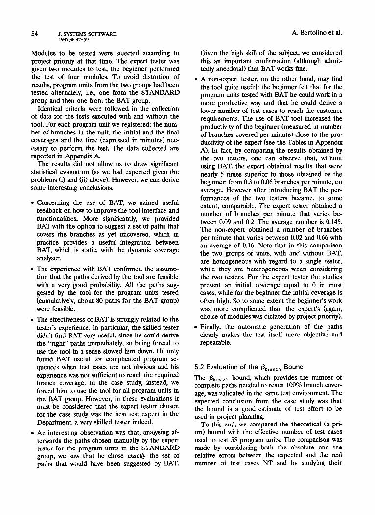
Table II. Expert Tester, Results WM BAT

Study Number of Initial branches coverage Final coverage

Time (minutes) Branch/min

EBl 52 EB2 16 EB3 5 EB4 5 EB5 3 EB6 23 EB7 15 EB8 13

0 0 0 0

6:22 66:67

0

98.08 300 0.17 93.75 160 0.09375

100 45 0.111111 84 25 0.2

100 30 0.1 100 45 0.177777 100 40 0.125 100 70 0.185714

of 0.09375 and a maximum of 0.2. The average number is 0.145419. In this case, the minimum (study EB2) and the maximum (study EB4) values of branch/minute are obtained for similar conditions: initial coverage equal to 0 and final coverage close to 90. Furthermore, the number of branches of the studies is different: 5 branches corresponding to the maximum value of branch/minute and 16 branches corresponding to the minimum.

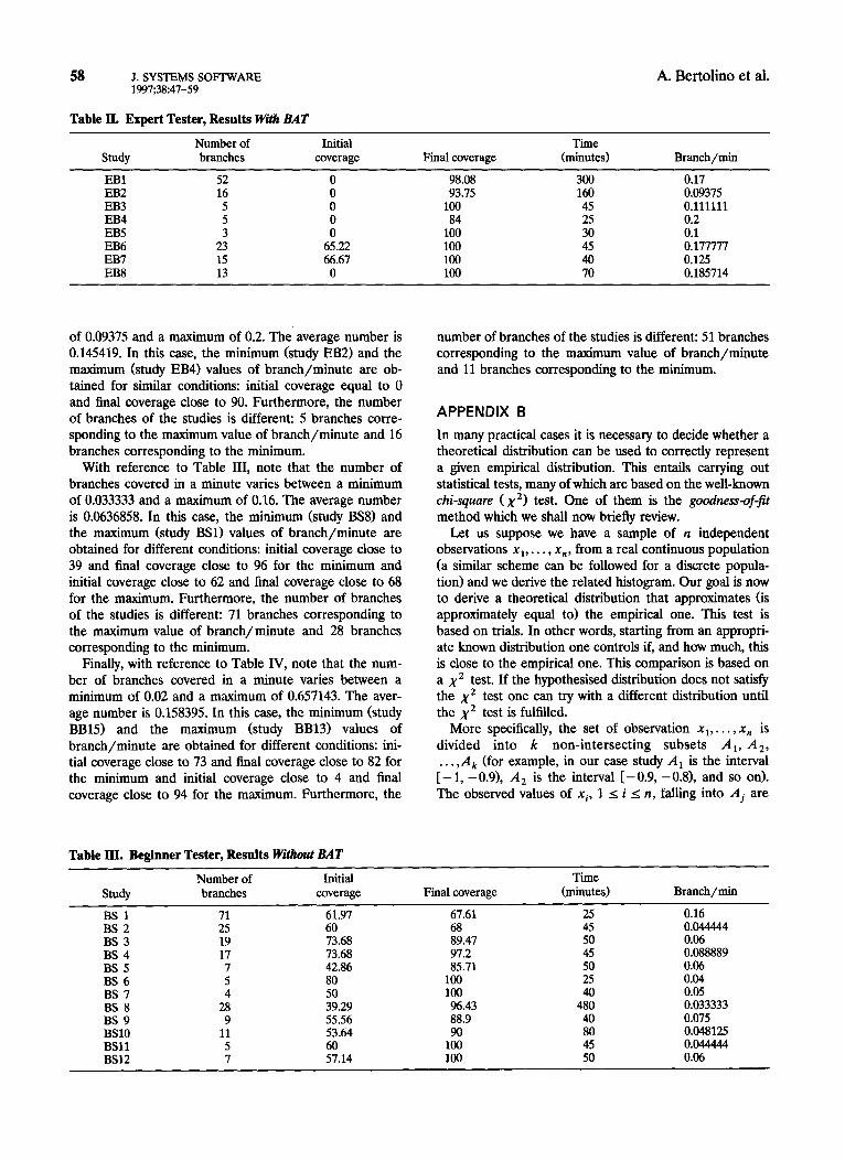
With reference to Table III, note that the number of branches covered in a minute varies between a minimum of 0.033333 and a maximum of 0.16. The average number is 0.0636858. In this case, the minimum (study BS8) and the maximum (study BSl) values of branch/minute are obtained for different conditions: initial coverage close to 39 and final coverage close to 96 for the minimum and initial coverage close to 62 and final coverage close to 68 for the maximum. Furthermore, the number of branches of the studies is different: 71 branches corresponding to the maximum value of branch/minute and 28 branches corresponding to the minimum.

Finally, with reference to Table IV, note that the number of branches covered in a minute varies between a minimum of 0.02 and a maximum of 0.657143. The average number is 0.158395. In this case, the minimum (study BB15) and the maximum (study BB13) values of branch/minute are obtained for different conditions: initial coverage close to 73 and final coverage close to 82 for the minimum and initial coverage close to 4 and final coverage close to 94 for the maximum. Furthermore, the

number of branches of the studies is different: 51 branches corresponding to the maximum value of branch/minute and 11 branches corresponding to the minimum.

APPENDIX B

In many practical cases it is necessary to decide whether a theoretical distribution can be used to correctly represent a given empirical distribution. This entails carrying out statistical tests, many of which are based on the well-known &i-square (~‘1 test. One of them is the goodness-of-fit method which we shall now briefly review.

Let us suppose we have a sample of n independent observations x 1,. . . , x,, from a real continuous population (a similar scheme can be followed for a discrete population) and we derive the related histogram. Our goal is now to derive a theoretical distribution that approximates (is approximately equal to) the empirical one. This test is based on trials. In other words, starting from an appropriate known distribution one controls if, and how much, this is close to the empirical one. This comparison is based on a x2 test. If the hypothesised distribution does not satisfy the x2 test one can try with a different distribution until the x2 test is fulfilled.

More specifically, the set of observation x1,. . . , x, is divided into k non-intersecting subsets Al, A,, . . . ,A, (for example, in our case study A, is the interval

[ - 1, - 0.9), A, is the interval [ - 0.9, - 0.81, and so on). The observed values of xi, 1 I i s n, falling into Aj are

Table III. Beginner Tester, Results WfI&out BAT

study

BS 1 BS 2 BS 3 BS 4 BS 5 BS 6 BS 7 BS 8 BS 9 BSlO BSll BS12

Number of Initial branches coverage

71 61.97 25 60 19 73.68 17 73.68 7 42.86 5 80 4 50

28 39.29 9 55.56

11 53.64 5 60 I 57.14

Final coverage

67.61 68 89.47 91.2 85.71

100 100 96.43 88.9 90

100 100

Time (minutes)

25 45 50 45 50 25 40

480 40 80 45 50

Branch/min

0.16 0.044444 0.06 0.088889 0.06 0.04 0.05 0.033333 0.075 0.048125 0.044444 0.06

A Case Study in Branch Testing Automation J. SYSTEMS SOFTWARE! 59 1997;38:47-59

Table IV. Beginner Tester, Results Wi BAT

Study

BB 1 BB 2 BB 3 BB 4 BB 5 BB 6 BB 7 BB 8 BB 9 BBlO BBll BB12 BB13 BB14 BB15

Number of Initial branches coverage

27 66.67 19 73.68 17 70.62 15 46.67 9 77.78 9 77.78 7 57.14 7 85.71

26 61.54 31 29.04 39 10.26 5 40

51 3.92 3 66.67

11 72.73

Final coverage

74.07 84.21 94.12 73.33

100 100 100 100 92.31

100 84.62

100 94.12

100 81.82

Time (minutes)

10 40 40 35 10 35 25 35

100 120 60 50 70 40 50

Branch/l&

0.2 0.05 0.1 0.114286 0.2 0.057143 0.12 0.02857 0.08 0.183333 0.483333 0.06 0.657143 0.025 0.02

then counted and the resulting number, also referred to as “observed quantities,” is denoted by 4. On this basis one can define a histogram (Figure 5 in the case study) that characterises the empirical distribution (Figure 6). As known, the sample mean is given by:

while the sample standard deviation by:

s2 = & ,i (Xi - ?)2. 1=1

Using these parameters one can define a normal distribution with mean 2 and standard deviation given by u

=G. The areas under the function and within each interval

represent the theoretical frequencies (also denoted as Fj, j = l,..., k) of observations if the distribution was really a normal distribution. The point is now to compare the empirical distribution with the normal distribution by use of the x2 test. The x2 statistic is defined as follows:

k IF_o\~

(1)

In the conventional case this variable is said to have df = k - 1 degrees of freedom because of the single relation existing between the observed frequencies: EF= ,4 = IZ. However, in this case, the number of degrees of freedom is reduced with respect to the conventional measure by a number of units equal to the parameters estimated by the sample, i.e., df = k - 1 - (number of estimated parameters).

For the normal distribution, that needs both the mean and the variance, the number of estimated parameters is equal to 2.

Before carrying out the test, a level of significance (Y must be decided upon. This is the probability of rejecting the hypothesis when it is, in fact, true.

The value of (Y should be small, but not too small (say ry = 0.1 or (Y = 0.05). It must be remembered that when

the likelihood of rejecting a true hypothesis decreases, that of accepting a false one increases (hence the term “level of confidence”).

Next, from a table of the x2 distribution, two points x1 and x2 are obtained:

In other words the value of ,y2 calculated from (1) will be within the interval (x,, x2) with probability 1 - (Y, if the hypothesis is true and in this case the empirical distribution can be approximated with a normal distribution with a level of confidence given by (1 - a)%. There- fore if (1) yields a value less than x1 or greater than x2 then the hypothesis ought to be rejected; the occurrence of an unlikely value argues against the hypothesis.

Note that there are some conditions under which it is appropriate to apply the x2 test.

First, the observations in the sample must be independent. Second, the size of the sample must be large. An accepted “rule of thumb” in this respect is that the expected number of observations in each subset should be at least 5 (for example, in the case study the test was applied to a number of categories k’ I k obtained by grouping the intervals in order to verify this hypothesis).

The Kolmogorov-Smimov (KS) test is based on a similar scheme, but unlike the x2 test, which requires quite a large set of observations, it can be applied to small observation samples. The test is based on the comparison between the observed and the theoretical cumulative distribution and, in particular, on the evaluation of the maximum difference between them. This value is then compared with some critical values reported in the KS table to decide if the hypothesised theoretical distribution can be accepted and with what level of confidence.

To summarise, the idea behind both the x2 test and the KS test is that the observed behaviour of a sample is compared with its hypothesised behaviour. If the agree- ment is suspiciously good (i.e., statistics less than x,) or suspiciously poor (i.e., statistics greater than x2), then the hypothesis is rejected, otherwise it is accepted.

Documents

A case study in branch testing automation