A BOUNDARY ELEMENT APPROACH FOR SHAPE AND …

A BOUNDARY ELEMENT APPROACH FOR SHAPE AND TOPOLOGY

DESIGN IN ORTHOTROPIC HEAT TRANSFER PROBLEMS

Carla Anflora and Rogério J. Marczak

b

Universidade Federal do Rio Grande do Sul, Sarmento Leite 425, 90430131 Porto Alegre, Brasil, a

[email protected], [email protected], http://www.ufrgs.br

Keywords: Topology optimization, heat transfer, Poisson equation, topological derivative, orthotropic materials, boundary element methods.

Abstract. A numerical approach for topology optimization of orthotropic potential problems using the boundary element methods (BEM) is introduced. The method is based on the evaluation of topological derivative, adopting the total potential energy as the cost function. A hard-kill algorithm is devised to progressively remove material where it is less necessary. This developed procedure is an alternative to the homogenization technique, avoiding the use of intermediary density material. The topology optimization of non-isotropic media is addressed using conformal mapping techniques. The method preserves BEM features, such as boundary-only discretization, reducing significantly the computational cost. Results obtained with the technique for Robin, Neumann and/or Dirichlet boundary conditions are compared and discussed with those available in the literature.

Mecánica Computacional Vol XXVII, págs. 2473-2486 (artículo completo)Alberto Cardona, Mario Storti, Carlos Zuppa. (Eds.)

San Luis, Argentina, 10-13 Noviembre 2008

Copyright © 2008 Asociación Argentina de Mecánica Computacional http://www.amcaonline.org.ar

1 INTRODUCTION

Most of the research on shape and topology optimization has focused on elasticity problems (BendsØe, 1995). The thermal conducting solid issue has received relatively less attention in spite of its significance. In this point of view, it makes necessary to investigate solids submitted to multiple flux loading, convection, with non-isotropic behavior, due its practical significance in the manufacturing industrial, such as, thermal molding-die, printed circuit boards (PCB) and diffusers. In recent years, a great deal of effort has been devoted to the development of various numerical techniques. Finite Element analysis associated with well known optimization methods (homogenization technique, evolutionary optimization) has become a widely used tool for engineers of many disciplines (BendsØe, 1995 and Li et al., 1999). Generally typical drawbacks are very common in optimization problems, such as, intermediary density, remesh, check-board instability. These drawbacks must be controlled, and sometimes, the final result does not discard a pos-processing which results an increase of computational cost.

Recently, a new family of methods based on topological derivative (DT) estimates or topological-shape sensibility (Sokolowski and Zochowski, 1997; Feijóo et al. 2003) has been proposed as an alternative to the homogenization methods. The main advantage of DT methods lies on the use of a constant density (avoiding intermediary materials) and easy implementation. On the other hand, it is quite difficult to be extended to more general cost functions and including problem dependent restrictions, as well (Garreau et al., 1998; Céa et al., 2000; Sokolowski and Zochowski, 2001; Feijóo, 2002; Novotny et al., 2003).

Significant reduction of computational costs has been attained by using BEM as solver in computational process, as optimization for example, since there is no mesh in the domain. So far, the BEM has been used mostly for shape optimization problems. Marczak (2005) introduced the application of a DT method using the boundary element method (BEM) applied to the topological optimization of linear isotropic potential problems.

The objective of the present work is to extend the proposed methodology in a previous work (Anflor and Marczak, 2006) which dealt with anisotropic solids submitted to heat transfer using DT, BEM and linear coordinate transformation. Now the idea concerns to apply that numerical methodology to study of the behavior of the solid design when a multi heat flux loading is introduced in the domain.

Firstly, the DT formulation focused on the Poisson equation is presented. Next, the heat source transfer treatment in BEM is briefly reviewed. Finally, a number of linear heat transfer problems are presented, being these results compared with those available in the literature.

C. ANFLOR, R. MARCZAK2474


2 TOPOLOGICAL DERIVATIVE REVIEW

Topological derivative for Poisson Equation is applied in this work. A simple example of applicability consists in a case where a small hole of radius (ε) is opened inside the domain. The concept of topological derivative consists in determining the sensitivity of a given function cost (ψ) when this small hole is increased or decreased. The local value of DT at a point ( x ) inside the domain for this case is evaluated by:

*

0

( ) ( )ˆ( ) lim

( )TD xf

ε

ε

ψ ψε→

Ω − Ω= (1)

Where ψ(Ω) and ψ(ε) are the cost function evaluated for the original and the perturbed domain, respectively, and “f” is a regularizing function. With equation (1) was not possible to establish an isomorphism between domains with different topologies. Feijóo et al. (2002) modified the equation introducing a mathematical idea that the creation of hole can be accomplished by single perturbing an existing one whose radius tends to zero. With this new way to state the problem it is possible to establish a mapping between each other (Novotny, 2003).

*

0

( ) ( )ˆ( ) lim

( ) ( )TD x

f fεε δε

εε δε

ψ ψε

+

→+

Ω − Ω=

Ω − Ω (2)

Where δε is a small perturbation on the radius of the hole. In the case of linear heat transfer, the direct problem is stated as:

Solve buku =∆− εε | on εΩ (3)

Subjected to

( )

( ), , 0

ε D

N

c ε R

u

n

u = u on Γ

uk = q on Γ

n

-k = h u -u on Γ

h on B

ε

εα β γ

∞

∂

∂

∂∂

= ∂

(4)

where:

( ) ( ), , 0c

Dirichlet Neumann Robin

u uh u u k q k h u u

n n

ε ε ε εε εε εα β γ α β γ ∞

∂ ∂= − + + + + − =

∂ ∂

(5)

Equation (5) is a function which takes into account the type of boundary condition on the

holes to be created ( ,u

u qnε

ε ε∂

=∂

are the temperature and flux on the hole boundary ( Bε∂ ),

while uε∞ and chε are the internal convection parameters of the hole, respectively).

After an intensive analytical work, Feijóo et al. (2002) have developed explicit expressions for DT for problems governed by Eq.(3). Table 1 presents these final expressions for topological derivative, considering the three classical cases of boundary conditions on the holes.

Mecánica Computacional Vol XXVII, págs. 2473-2486 (2008) 2475


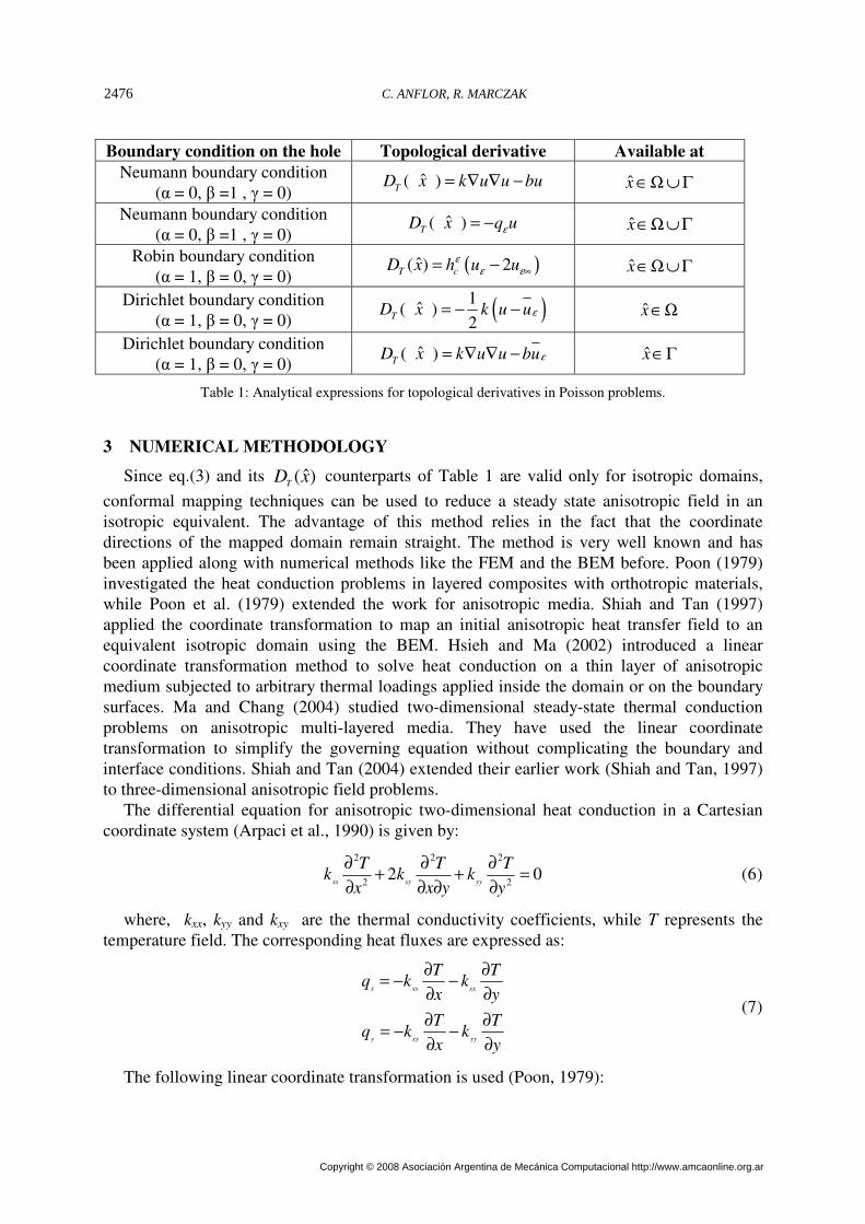
Boundary condition on the hole Topological derivative Available at

Neumann boundary condition (α = 0, β =1 , γ = 0)

ˆ( )T

D x k u u bu= ∇ ∇ − x ∈Ω ∪ Γ

Neumann boundary condition (α = 0, β =1 , γ = 0)

ˆ( )T

D x q uε= − x∈Ω ∪Γ

Robin boundary condition (α = 1, β = 0, γ = 0)

( )ˆ( ) 2T cD x h u uε

ε ε∞= − x∈Ω ∪Γ

Dirichlet boundary condition (α = 1, β = 0, γ = 0)

( )1ˆ( )

2T

D x k u uε= − − x∈Ω

Dirichlet boundary condition (α = 1, β = 0, γ = 0)

ˆ( )T

D x k u u buε= ∇ ∇ − x∈Γ

Table 1: Analytical expressions for topological derivatives in Poisson problems.

3 NUMERICAL METHODOLOGY

Since eq.(3) and its ˆ( )T

D x counterparts of Table 1 are valid only for isotropic domains,

conformal mapping techniques can be used to reduce a steady state anisotropic field in an isotropic equivalent. The advantage of this method relies in the fact that the coordinate directions of the mapped domain remain straight. The method is very well known and has been applied along with numerical methods like the FEM and the BEM before. Poon (1979) investigated the heat conduction problems in layered composites with orthotropic materials, while Poon et al. (1979) extended the work for anisotropic media. Shiah and Tan (1997) applied the coordinate transformation to map an initial anisotropic heat transfer field to an equivalent isotropic domain using the BEM. Hsieh and Ma (2002) introduced a linear coordinate transformation method to solve heat conduction on a thin layer of anisotropic medium subjected to arbitrary thermal loadings applied inside the domain or on the boundary surfaces. Ma and Chang (2004) studied two-dimensional steady-state thermal conduction problems on anisotropic multi-layered media. They have used the linear coordinate transformation to simplify the governing equation without complicating the boundary and interface conditions. Shiah and Tan (2004) extended their earlier work (Shiah and Tan, 1997) to three-dimensional anisotropic field problems.

The differential equation for anisotropic two-dimensional heat conduction in a Cartesian coordinate system (Arpaci et al., 1990) is given by:

2 2 2

2 22 0

xx xy yy

T T Tk k k

x x y y

∂ ∂ ∂+ + =

∂ ∂ ∂ ∂ (6)

where, kxx, kyy and kxy are the thermal conductivity coefficients, while T represents the temperature field. The corresponding heat fluxes are expressed as:

x xx xx

y xy yy

T Tq k k

x y

T Tq k k

x y

∂ ∂= − −

∂ ∂

∂ ∂= − −

∂ ∂

(7)

The following linear coordinate transformation is used (Poon, 1979):



ˆ 1

ˆ 0

x x

y y

α = β

(8)

where /xy yy

k k−α = , / yyk kβ = , and 2

xx yy xyk k k k= − . Now the governing equation in the

transformed domain reads:

2 2

2 20

ˆ ˆ

T Tk

x y

∂ ∂+ =

∂ ∂ (9)

where k is the equivalent thermal conductivity. Equation (9) now resembles eq.(3), i.e. an

equivalent isotropic problem. It is interesting to point out that when 0xy

k = , the

transformation of eq.(8) is merely a rotation of the constitutive coordinate system to its principal directions. Neumann boundary conditions also must be transformed accordingly:

ˆ

ˆ ˆ

y y

x x y

Tq k q

y

q q q

∂= − =

∂

= β − α (10)

By inverting the eq.(10), the Neumann boundary conditions are promptly recovered as a function of the original domain boundary conditions.

ˆ

ˆ

yy

x y

x

q q

q qq

=

+ α=

β

(11)

In the present work, the boundary element method was used as numerical method to solve the governing equations. The boundary integral equation for problems governed by eq.(3) is given by (Kane, 1994):

* * *ˆ ˆ ˆ ˆ ˆ ˆ ˆ ˆ ˆ ˆ ˆ( ) ( ) ( , ) ( ) ( , ) ( ) ( , ) ( )c x T x q x y T y d T x y q y d T x y b y dΓ Γ Ω

+ Γ = Γ + Γ∫ ∫ ∫ (12)

where c is the geometric factor of the boundary point x , T and q are the temperatures and

the fluxes on the boundary Γ, respectively, and b is the heat generated inside the domain Ω.

The symbols *T and *

q refer to the temperature and flux fundamental solutions for an infinite

medium:

( )* 1ˆ ˆ ˆ ˆ( , ) ln

2T x y x y

kt

−= −

π (13)

* *ˆ ˆ ˆ ˆ ˆ( , ) ( , ) ( )q x y k T x y y= − ∇ ⋅n

where t is the thickness of the medium and n is the outward normal of the boundary Γ at y . In the cases where there are n heat sources of intensity s inside the domain, placed at

coordinates z , the last term of eq.(12) can be particularized by replacing b for a concentrated heat source (Kamiya and Sawaki, 1985):

1

ˆ ˆˆ ˆ( ) ( ) ( , )n

i i

i

b y s z y z=

= δ∑ (14)

and eq.(12) is rewritten as:



* * *

1

ˆ ˆ ˆ ˆ ˆ ˆ ˆ ˆ ˆ ˆ ˆ( ) ( ) ( , ) ( ) ( , ) ( ) ( , ) ( )n

i

i

c x T x q x y T y d T x y q y d T x z s z=Γ Γ

+ Γ = Γ +∑∫ ∫ (15)

where x ∈Γ . After the usual discretization of the boundary Γ in boundary elements, and

parameterization of the temperature and fluxes through interpolation functions, eq.(15) is applied to each boundary nodal point x , generating the system of equations:

= +HT GQ f (16)

where the vectors T and Q contains the temperature and fluxes of the boundary nodes, while the last term on the right side contains the heat sources contribution. Since at each

nodal point on Γ whether the temperature or the normal heat flux is known, the columns

of eq.(16) can be exchanged to group the boundary unknowns in a single vector X:

AX = B (16)

Once the system of equations (16) is solved, all the boundary variables are known, and the temperature on interior points can be recovered as a post-processing step, using the integral equation for temperatures are internal points (Kane, 1994):

* * *

1

ˆ ˆ ˆ ˆ ˆ ˆ ˆ ˆ ˆ ˆ( ) ( , ) ( ) ( , ) ( ) ( , ) ( )n

i

i

T x T x y q y d q x y T y d T x z s z=Γ Γ

= Γ − Γ +∑∫ ∫ (17)

where x ∈Ω .

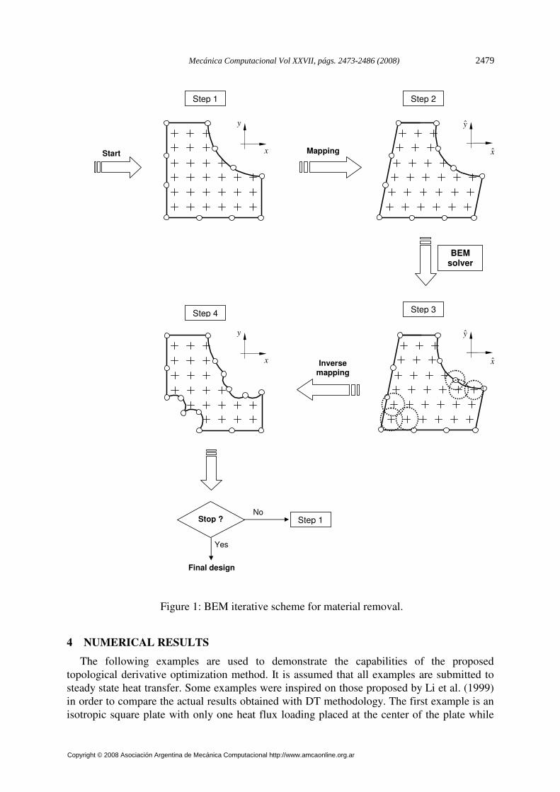
In order to adapt a BEM code based on eqs.(15) and (17) for topology optimization of orthotropic media, the following algorithm was implemented (see fig.1):

1. Start with the orthotropic domain mesh and a suitable grid of internal points. 2. Transform an orthotropic domain into an equivalent isotropic one by the linear

coordinate transformation given by eq.(8). The Neumann b.c., the coordinates of internal points and the heat sources inside the domain also must be transformed. Solve the problem by the BEM as an isotropic case.

3. The variables are evaluated on all interior points. The points with the lowest values of

TD are selected.

4. Apply the inverse mapping. Holes are created by punching out disks of material centered on the previously selected points. Check stopping criteria, rebuilt the mesh and return to step 1, if necessary. When the process is halted, an optimal topology is expected.

The grid of internal points is generated automatically, taking into account the radius of the holes created during each iteration. Different patterns of internal points can be generated, as discussed by Marczak (2007). In addition, the analyst can restrict the grid to the design areas only, reducing significantly the computational overhead. The radius of the holes are taken as a

fraction of a reference dimension of the original domain ( refr l= λ ), where

ref min(height,width)l = is generally adopted. The current area of the domain (f

A ) is checked

at the end of each iteration until the target value is achieved ( 0fA A= ξ , where 0A is the initial

area).



BEM solver

Mapping

Inverse mapping

Stop ?

Step 1 Step 2

Step 3 Step 4

Yes

No Step 1

Final design

Start

y

x

y

x

y

x

y

x

Figure 1: BEM iterative scheme for material removal.

4 NUMERICAL RESULTS

The following examples are used to demonstrate the capabilities of the proposed topological derivative optimization method. It is assumed that all examples are submitted to steady state heat transfer. Some examples were inspired on those proposed by Li et al. (1999) in order to compare the actual results obtained with DT methodology. The first example is an isotropic square plate with only one heat flux loading placed at the center of the plate while



the second one refers to an isotropic rectangular plate with two heat fluxes loading in the domain. The third example consists in an isotropic PCB (printed circuit board) with four heat flux loading, what represents some electronics components who generates heat. The fourth example presents a comparative between the final design provided by an isotropic and an orthotropic media. All examples are compared with those available in the literature. The material removal history is analyzed and illustrated for each case. The iterative process was halted when a given amount of material is removed from the original domain, regardless the type of material medium. This provided a basis to compare the topologies generated for isotropic, orthotropic and anisotropic media under the same initial geometry and boundary conditions. In all cases the total potential energy was used as the cost function. A regularly spaced grid of internal points was generated automatically, taking into account the radius of the holes created during each iteration. The radius was taken as a fraction of a reference dimension of the domain (r = α lref). Usually lref = min(height,width) was adopted. The objective in all cases is to minimize the material volume. The current area of the domain (Af) was checked at the end of each iteration until a reference value is achieved (Af = βA0, where A0 represents the initial area). Linear discontinuous boundary elements integrated with 4 Gauss points were used in all cases.

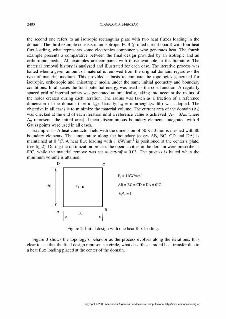
Example 1 – A heat conductor field with the dimension of 50 × 50 mm is meshed with 80 boundary elements. The temperature along the boundary (edges AB, BC, CD and DA) is maintained at 0 °C. A heat flux loading with 1 kW/mm2 is positioned at the center’s plate, (see fig.2). During the optimization process the open cavities in the domain were prescribe as 0°C, while the material remove was set as cut-off = 0.03. The process is halted when the minimum volume is attained.

Figure 2: Initial design with one heat flux loading. Figure 3 shows the topology’s behavior as the process evolves along the iterations. It is

clear to see that the final design represents a circle, what describes a radial heat transfer due to a heat flux loading placed at the center of the domain.

F1 = 1 kW/mm2

AB = BC = CD = DA = 0°C kx/ky = 1

50

50

F1

A B

C D



Figure 3: Historic evolution: one heat flux loading.

Example 2 – This case is similar to the previous one, except that kx/ky = 2 is imposed. In Figure 4 is possible to accomplish the iterative process and verify that an elliptical profile is obtained as a final result. An elliptical profile as a final shape is justified due to a non-isotropic feature of the material. It is interpreted as the heat transfers faster in direction x, and the material remained in this direction is of higher conductivity efficiency.

Figure 4: Historic evolution for orthotropic case with one heat flux loading.

Iteration #5

Iteration #16 Iteration #11

Iteration #9

Iteration #18 Iteration # 32

Iteration # 45 Iteration # 56



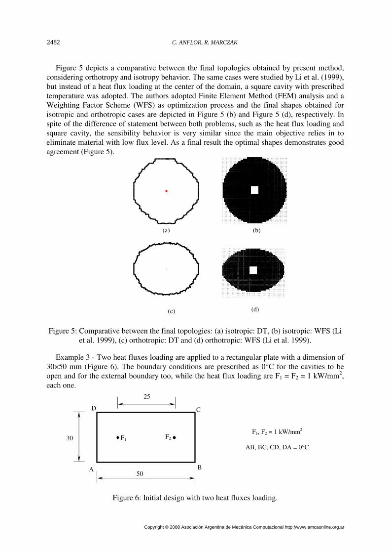
Figure 5 depicts a comparative between the final topologies obtained by present method, considering orthotropy and isotropy behavior. The same cases were studied by Li et al. (1999), but instead of a heat flux loading at the center of the domain, a square cavity with prescribed temperature was adopted. The authors adopted Finite Element Method (FEM) analysis and a Weighting Factor Scheme (WFS) as optimization process and the final shapes obtained for isotropic and orthotropic cases are depicted in Figure 5 (b) and Figure 5 (d), respectively. In spite of the difference of statement between both problems, such as the heat flux loading and square cavity, the sensibility behavior is very similar since the main objective relies in to eliminate material with low flux level. As a final result the optimal shapes demonstrates good agreement (Figure 5).

Figure 5: Comparative between the final topologies: (a) isotropic: DT, (b) isotropic: WFS (Li et al. 1999), (c) orthotropic: DT and (d) orthotropic: WFS (Li et al. 1999).

Example 3 - Two heat fluxes loading are applied to a rectangular plate with a dimension of 30×50 mm (Figure 6). The boundary conditions are prescribed as 0°C for the cavities to be open and for the external boundary too, while the heat flux loading are F1 = F2 = 1 kW/mm2, each one.

Figure 6: Initial design with two heat fluxes loading.

F1, F2 = 1 kW/mm2

AB, BC, CD, DA = 0°C

30

50

F2 F1

C

B A

D

25

(a) (b)

(d)

(c)



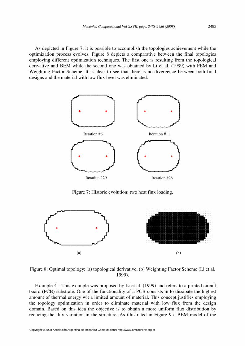
As depicted in Figure 7, it is possible to accomplish the topologies achievement while the

optimization process evolves. Figure 8 depicts a comparative between the final topologies employing different optimization techniques. The first one is resulting from the topological derivative and BEM while the second one was obtained by Li et al. (1999) with FEM and Weighting Factor Scheme. It is clear to see that there is no divergence between both final designs and the material with low flux level was eliminated.

Figure 7: Historic evolution: two heat flux loading.

Figure 8: Optimal topology: (a) topological derivative, (b) Weighting Factor Scheme (Li et al. 1999).

Example 4 - This example was proposed by Li et al. (1999) and refers to a printed circuit board (PCB) substrate. One of the functionality of a PCB consists in to dissipate the highest amount of thermal energy wit a limited amount of material. This concept justifies employing the topology optimization in order to eliminate material with low flux from the design domain. Based on this idea the objective is to obtain a more uniform flux distribution by reducing the flux variation in the structure. As illustrated in Figure 9 a BEM model of the

(a) (b)





PCB substrate is designed with a mesh of 32 elements. Four steady heat flux loading F1, F2, F3 and F4 are set to 1kW/mm2, which are generated by several major electronic components mounted on the PCB. The structure consists of design and non-design domains as shown in Figure 4.9. The temperature on the boundary (edges AB, BC, CD and DA) is maintained at 0°C throughout evolution process. For the cavities to be open is prescribed Neumann homogeneous as boundary condition. The process is halted when a volume ratio of 68% is attained.

Figure 9: Initial design for PCB.

Throughout Figure 10, it is possible to accomplish the historical evolution for this PCB

case. Clearly, the material who presents a low efficiency in heat transfer is gradually removed. After an amount of material has done removed at the center, the next areas with low efficiency are the rectangle’s corners as depicted at iteration 27 in Figure 10.

Figure 10: Evolution history.

B

C

53

F1

F2

F3

F4

F1, F2, F3, F4 = 1 kW/mm2

AB, BC, CD, DA = 0°C

Non- design domain

33

A

D

Iteration #27


Iteration # 24



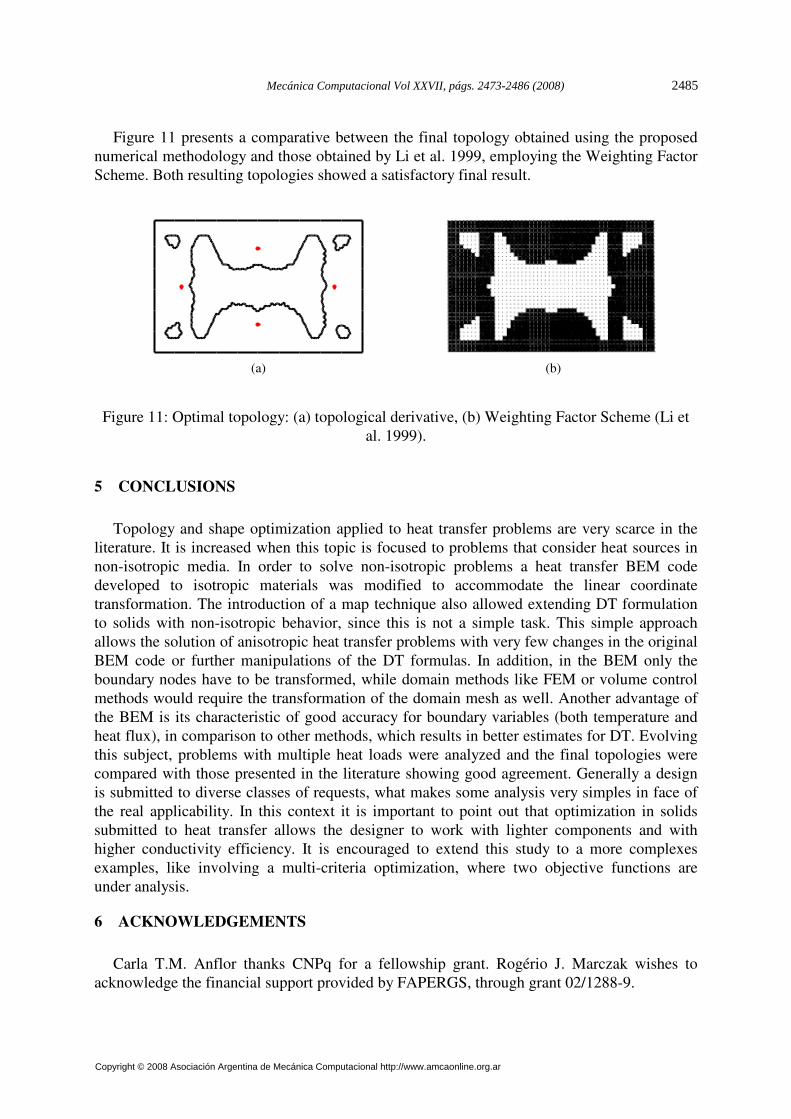
Figure 11 presents a comparative between the final topology obtained using the proposed numerical methodology and those obtained by Li et al. 1999, employing the Weighting Factor Scheme. Both resulting topologies showed a satisfactory final result.

Figure 11: Optimal topology: (a) topological derivative, (b) Weighting Factor Scheme (Li et al. 1999).

5 CONCLUSIONS

Topology and shape optimization applied to heat transfer problems are very scarce in the literature. It is increased when this topic is focused to problems that consider heat sources in non-isotropic media. In order to solve non-isotropic problems a heat transfer BEM code developed to isotropic materials was modified to accommodate the linear coordinate transformation. The introduction of a map technique also allowed extending DT formulation to solids with non-isotropic behavior, since this is not a simple task. This simple approach allows the solution of anisotropic heat transfer problems with very few changes in the original BEM code or further manipulations of the DT formulas. In addition, in the BEM only the boundary nodes have to be transformed, while domain methods like FEM or volume control methods would require the transformation of the domain mesh as well. Another advantage of the BEM is its characteristic of good accuracy for boundary variables (both temperature and heat flux), in comparison to other methods, which results in better estimates for DT. Evolving this subject, problems with multiple heat loads were analyzed and the final topologies were compared with those presented in the literature showing good agreement. Generally a design is submitted to diverse classes of requests, what makes some analysis very simples in face of the real applicability. In this context it is important to point out that optimization in solids submitted to heat transfer allows the designer to work with lighter components and with higher conductivity efficiency. It is encouraged to extend this study to a more complexes examples, like involving a multi-criteria optimization, where two objective functions are under analysis.

6 ACKNOWLEDGEMENTS

Carla T.M. Anflor thanks CNPq for a fellowship grant. Rogério J. Marczak wishes to acknowledge the financial support provided by FAPERGS, through grant 02/1288-9.

(a) (b)



REFERENCES

Anflor, C., Marczak R., Topology optimization and boundary elements: application of topological derivatives to solve potential problems in orthotropic materials. Proceedings of

the 11th Brazilian Congress of Thermal Sciences and Engineering - ENCIT 2006 Braz. Soc.

of Mechanical Sciences and Engineering - ABCM, Curitiba, Brazil, Dec. 5-8, 2006. Arpaci, V.S., Selamet, A., Kao S.H., Introduction to Heat Transfer, second ed., Prentice-

Hall, New York, 2000. Bendsøe, M. P., Optimization of Structural Topology, Shape, and Material, Springer-Verlag,

Berlin, 1995. Brebbia, C. A. and Dominguez, J., Boundary Elements an Introductory Course, Ed. McGraw-

Hill, New York, United States, 1992. Céa J., Garreau, S., Guillaume P., Masmoudi, M., The shape and topological optimizations

connection, Comput. Methods Appl. Mech. Engrg. 188:713-726, 2000. Feijóo, R., Novotny,A., Taroco, E., & Padra, C., The topological derivative for the poisson’s

problem, Mathematical Models and Methods in Applied Sciences, 13:1825-1844, 2003. Feijóo, R., Novotny, A., Padra, C & Taroco, E., The topological-shape sensitivity analysis and

its appications in optimal design, In Idelsohn, S., Sonzogni, V., & Cardona, A., eds. Mecánica Computacional, volume XXI, pp. 2687-2711, Santa-Fé-Paraná, Argentina, 2002.

Garreau, S., Guillaume, P.& Masmoudi, M., The topological gradient. Research report, Université Paul Sabatier, Toulouse 3, France, 1998.

Kamiya, N., Sawaki, Y., An Efficient BEM for Some Inhomogeneous and Nonlinear Problems, in: Brebbia, C.A. and Maier, G. (Eds.) Proceedings of the Seventh Int. Sem. BEM

Eng., Villa Olmo, Italy, 1985, pp. 13-68 Kane, J.H., Boundary element analysis in engineering continuum mechanics, Prentice-Hall,

New Jersey, 1994. Li, Q., Steven, G., Querin, O., & Xie, Y., Shape and topology design for heat conduction by

evolutionary structural optimization, Int. J. Heat and Mass Transfer, 42:3361-3371, 1999. Marczak, R.J., Topology Optimization and Boundary Elements – A Preliminary

Implementation for Linear Heat Transfer, XXVI Iberian Latin-American Congress on

Computational Methods in Engineering - CILAMCE 2005, Brazilian Assoc. for Comp. Mechanics & Latin American Assoc. of Comp. Methods in Engineering, Guarapari - ES, Brazil, 2005.

Marczak, R.J., Topology Optimization and Boundary Elements – A Preliminary Implementation for Linear Heat Transfer, Engineering Analysis with Boundary Elements, 31:793-802, 2007.

Novotny, A., Feijóo, R., Taroco, E., Padra, C., Topological-shape sensitivity analysis, Comput. Methods Appl. Mech. Engrg., 192:803–829, 2003.

Sokolowski, J., Zochowski, A., On topological derivative in shape optimization, Research Report 3170, INRIA-Lorraine, France, 1997.

Sokolowski, J., Zochowski, A., Topological derivatives of shape functional for elasticity systems”, Mech. Struct. Mach., 29:331-349, 2001.



Documents

A BOUNDARY ELEMENT APPROACH FOR SHAPE AND …