A Behavioral Explanation for the Puzzling Persistence of

ESRI Discussion Paper Series No.360

A Behavioral Explanation for the Puzzling Persistence of the Aggregate Real Exchange Rate

Mario J. Crucini, Mototsugu Shintani, and Takayuki Tsuruga

March 2021

Economic and Social Research Institute

Cabinet Office

Tokyo, Japan

The views expressed in “ESRI Discussion Papers” are those of the authors and not those of the Economic and Social Research Institute, the Cabinet Office, or the Government of Japan. (Contact us: https://form.cao.go.jp/esri/en_opinion-0002.html)

A Behavioral Explanation for the Puzzling Persistence of

the Aggregate Real Exchange Rate∗

Mario J. Crucini†, Mototsugu Shintani‡and Takayuki Tsuruga§

This version: December 2020

Abstract

At the aggregate level, the evidence that deviations from purchasing power parity

(PPP) are too persistent to be explained solely by nominal rigidities has long been a

puzzle (Rogoff, 1996). Another puzzle from the micro price evidence of the law of one

price (LOP), which is the basic building block of PPP, is that LOP deviations are less

persistent than PPP deviations. To reconcile the empirical evidence, we adapt the model

of behavioral inattention in Gabaix (2014, 2020) to a simple two-country sticky-price

model. We propose a simple test of behavioral inattention and find strong evidence in

its favor using micro price data from US and Canadian cities. Calibrating behavioral

inattention with our estimates, we show that our model reconciles the two puzzles relat-

ing to the PPP and LOP. First, the PPP deviations are more than twice as persistent as

PPP deviations explained only by sticky prices. Second, the LOP deviations decrease

to less than two-thirds of the PPP deviations in the degree of persistence.

JEL Classification: E31; F31; D40

Keywords: Real exchange rates, Law of one price, Rational inattention, Trade cost

∗We thank David Cook, Mick Devereux, Ippei Fujiwara, Yasuo Hirose, Jinill Kim, Akihisa Shibata, KwanhoShin and conference and seminar participants at the 5th International Macroeconomics and Finance Confer-ence, Keio University, Otaru University of Commerce, Tokyo Institute of Technology, The University of Tokyo,and Vanderbilt University for their helpful comments and suggestions. Mototsugu Shintani and Takayuki Tsu-ruga gratefully acknowledge the financial support of Grant-in-aid for Scientific Research (15H05728, 15H05729,17H02510, and 18K01684), the Joint Usage/Research Center at the Institute of Social and Economic Research(Osaka University), the Kyoto Institute of Economic Research (Kyoto University), and the International JointResearch Promotion Program in Osaka University.

†Department of Economics, Vanderbilt University and NBER.‡Faculty of Economics, The University of Tokyo.§Institute of Social and Economic Research, Osaka University; and CAMA.

1

ESRI Discussion Paper Series No.360 "A Behavioral Explanation for the Puzzling Persistence of the Aggregate Real Exchange Rate"

1 Introduction

It is well known that the aggregate real exchange rate, namely the deviation from purchasing

power parity (PPP), is highly persistent. In a description of this empirical anomaly known

as the PPP puzzle, Rogoff (1996) states “Consensus estimates for the rate at which PPP

deviations damp, however, suggest a half-life of three to five years, seemingly far too long

to be explained by nominal rigidities” (p. 648). A closely related empirical fact of real

exchange rates is the gap in persistence between the PPP deviations and the deviations from

the law of one price (LOP), as the basic building block for PPP. For example, Imbs et al.

(2005) and Carvalho and Nechio (2011) argue that the aggregate real exchange rate (the PPP

deviations) is likely to be much more persistent than the good-level real exchange rate (the

LOP deviations).1 These previous studies emphasize the role of heterogeneity in the speed

of price adjustment. As Imbs et al. (2005) argued, “It is this heterogeneity that we find to

be an important determinant of the observed real exchange rate persistence since it gives rise

to highly persistent aggregate series while relative price persistence is low on average at a

disaggregated level” (p. 3).

In this paper, we aim to explain two empirical anomalies simultaneously: (1) the gap

between the observed persistence of the PPP deviations and the persistence predicted from

the sticky-price model (e.g., Rogoff, 1996); and (2) the gap between the observed persistence

of the PPP deviations and the LOP deviations (e.g., Imbs et al., 2005). To this end, we

incorporate behavioral inattention along the lines of Gabaix (2014, 2020) into a simple two-

country sticky-price model. In this framework, firm managers bear the cost of paying attention

to the aggregate component of the marginal cost of their products. As a result, the full

attention to the state of the economy is no longer optimal when firms choose the prices of

goods.

The key to solving the PPP puzzle is the complementarity between the LOP and PPP

deviations. After deriving a reduced-form solution for the LOP deviations, we show that the

LOP deviations are affected by the PPP deviations when firms pay only partial attention

to marginal cost. Thus, an increase in the persistence of the PPP deviations makes the

LOP deviations more persistent. At the same time, through the aggregation, the more

persistent LOP deviations lead to more persistent PPP deviations, further strengthening the

link between the PPP and LOP deviations.

1See Crucini and Shintani (2008) for a comprehensive empirical analysis of the persistence in the LOPdeviations.

2


The reduced-form solution leads to a direct testable implication. Using US and Canadian

micro price data, we implement a simple test for the null hypothesis of full attention against

an alternative hypothesis of partial attention. This test is equivalent to asking whether the

good-level real exchange rate is uncorrelated with the aggregate real exchange rate after

controlling for the common driving forces, such as the nominal exchange rate and country-

specific productivity. Using various specifications, we strongly reject the null in favor of our

proposed model of behavioral inattention. We also find the estimated degree of attention to

be around 0.17, much less than the value of 1.0 under full attention.

In the first theoretical result, our model of behavioral inattention ensures that the persis-

tence in the aggregate real exchange rate exceeds the persistence implied solely by nominal

rigidities. While the setting differs greatly, this mechanism is consistent with Ball and Romer

(1990) and Woodford (2003), who show that even small frictions in nominal price adjustment

lead to a persistent output gap when real rigidities or strategic complementarities are present.

In our model with behavioral inattention, only small nominal frictions are needed to generate

a highly persistent aggregate real exchange rate. Based on our estimates of the degree of

attention, the persistence of the aggregate real exchange rate rises to 0.74 from 0.34 in the

full attention case.

In the second theoretical result of our model, we explain the gap between the highly

persistent PPP deviations and the less persistent LOP deviations. This gap arises from the

combination of the complementarity and the presence of idiosyncratic real shocks to the

individual price of goods. We show that both the aggregate and the good-level real exchange

rates are more persistent when complementarities are present. In contrast, real shocks at

the good level (but not country-specific real shocks) reduce persistence only for the LOP

deviations and not for the PPP deviations. This is because the aggregation across goods

eliminates the effect of real shocks at the good level. As a result, our estimates of the degree

of attention also imply a substantial gap in persistence between the PPP and LOP deviations.

In fact, we predict the persistence of the LOP deviations to be 57 percent lower than the

persistence of the PPP deviations.

Our results relate to an extensive literature that has contributed to a better understanding

of persistent aggregate real exchange rates. For instance, Chari et al. (2002) argue that while

the sticky-price model can explain the volatility of the aggregate real exchange rate, the

persistence is less than that suggested by the data. Benigno (2004) emphasizes the role of

monetary policy rules rather than the degree of price stickiness in accounting for the persistent

aggregate real exchange rate. Later, Engel (2019) revisits Benigno (2004) and argues for the

3


importance of both monetary policy rules and price stickiness. Blanco and Cravino (2020)

introduce a concept of the real exchange rate using only newly reset prices and find that this

“reset” exchange rate explains almost all fluctuations in the aggregate real exchange rate. Our

solution also closely relates to Bergin and Feenstra (2001) and Kehoe and Midrigan (2007),

who introduce strategic complementarity in pricing to two-country sticky-price models in

explaining the high persistence of real exchange rates. Our explanation of the PPP puzzle

does not rule out these explanations. Instead, we focus on the importance of behavioral

inattention in pricing of firms.

A popular explanation for the gap in persistence between aggregate (CPI-based) and

good-level real exchange rates is the heterogeneity in price adjustment at a good level, which

generates a positive bias when aggregating prices. Imbs et al. (2005) point out a positive

aggregation bias in dynamic heterogeneous panels, and Carvalho and Nechio (2011) consider

the theoretical implication of aggregation based on the sticky-price model in which the degree

of price stickiness differs across sectors. Indeed, both statistical aggregation bias and multi-

sector sticky-price models would help toward increasing the persistence of real exchange rates.

In contrast, our solution can explain the gap even if the persistence of the LOP deviations

is restricted to be common across goods. In this sense, the mechanism in our paper further

enhances the ability of existing workhorse models in the macroeconomics literature.

The remainder of the paper is structured as follows. In Section 2, we present a simple

two-country open economy model with Calvo pricing and introduce behavioral inattention.

Section 3 introduces the reduced-form solution for the LOP deviations and discusses the

implications of behavioral inattention. In Section 4, we implement a test of behavioral inat-

tention and quantify its importance. In Section 5, we assess how much the estimated degree

of behavioral inattention can improve model predictions. Section 6 concludes.

2 The model

The economy consists of two countries. In what follows, the US and Canada represent the

home and foreign countries, respectively. Following Kehoe and Midrigan (2007) and Crucini et

al. (2010b, 2013), there is a continuum of goods and brands of each good. Goods are indexed

by i and brands are indexed by z. For each good, US brands are indexed by z ∈ [0, 1/2] and

Canadian brands are indexed by z ∈ (1/2, 1].

We assume that US and Canadian consumers have identical preferences over brands of

a particular good and also across goods in the aggregate consumption basket. US prefer-

4


ences over the brands of good i are given by the constant elasticity-of-substitution (CES)

index for good i ∈ [0, 1]. The US consumption of good i is cit =[∫ 1

z=0cit(z)

ε−1ε dz

] εε−1

and the aggregation across goods gives aggregate consumption ct =[∫ 1

i=0cit

ε−1ε di

] εε−1

, where

ε > 1. For Canada, we have the analogous equations c∗it =[∫ 1

z=0c∗it(z)

ε−1ε dz

] εε−1

and

c∗t =[∫ 1

i=0c∗it

ε−1ε di

] εε−1

.

2.1 Households

The objective of the US agent is to maximize E0

∑∞t=0 δ

tU(ct, nt) = E0

∑∞t=0 δ

t(ln ct − χnt),subject to the budget constraint given by:

Mt + Et(∆t,t+1Bt+1) = Wtnt +Bt +Mt−1 − Pt−1ct−1 + Tt + Πt, (1)

and a cash-in-advance (CIA) constraint, Mt ≥ Ptct. Here, E0(·) denotes the expectation

operator conditional on the information available in period 0, δ ∈ (0, 1), and χ > 0. In

addition, we suppress the state contingencies for notational convenience. On the right-hand

side of the budget constraint (1), the household supplies hours worked nt, receives nominal

wages Wt for hours worked, carries bonds Bt into period t, as well as any cash that remained

in period t− 1, Mt−1 − Pt−1ct−1. The household also receives nominal transfers from the US

government, Tt, and nominal profits from US firms, Πt. In (1), the aggregate price Pt is given

by Pt =[∫P 1−εit di

] 11−ε , where Pit is the price index for good i. This is a CES aggregate over

brands: Pit =[∫Pit(z)1−εdz

] 11−ε . The left-hand side of (1) represents the nominal value of

the total wealth of the household. The household allocates the wealth into state-contingent

nominal bond holdings Bt+1 brought into period t + 1 and money balances Mt. The CIA

constraint requires nominal money balances for expenditure which is made at the end of the

period t. The CIA always binds with equality in equilibrium.

Canadian households solve the analogous maximization problem. We assume complete

markets for state-contingent financial claims across the US and Canada and the financial

claims are denominated in US dollars. Thus, we convert their US dollar bond holdings into

Canadian dollars at the spot nominal exchange rate, St. The Canadian households are subject

to budget constraint,

M∗t +

Et(∆t,t+1B∗t+1)

St= W ∗

t n∗t +

B∗tSt

+M∗t−1 − P ∗t−1c∗t−1 + T ∗t + Π∗t . (2)

5


and the CIA constraint, M∗t ≥ P ∗t c

∗t .

The first-order conditions are standard. For the US households, we have Wt/Pt = χct

and ∆t,t+1 = δ[(ct+1/ct)−1(Pt/Pt+1)], where ∆t,t+1 is the nominal stochastic discount factor.

For Canadian households, we have W ∗t /P

∗t = χc∗t and ∆t,t+1 = δ[(c∗t+1/c

∗t )−1StP

∗t /(St+1P

∗t+1)].

The consumption Euler equations differ because Canadians buy state-contingent bonds de-

nominated in US dollars.

Define the aggregate real exchange rate as qt = StP∗t /Pt. The Euler equations imply

qt+1(c∗t+1/ct+1) = qt(c

∗t/ct) = ... = q0(c

∗0/c0). Normalizing q0(c

∗0/c0) to unity yields2

qt =

(ctc∗t

). (3)

2.2 Firms

The US firm specializes in the production of brand z ∈ [0, 1/2] of good i and employs nit(z)

hours of labor. They will produce output according to the production function yit(z) =

aitnit(z), where ait is labor productivity specific to good i and to all US firms that produce

that good. US firms produce brands on the first-half of the unit continuum, z ∈ [0, 1/2].

Thus, for example, all firms that produce beer in the US share the same labor productivity.

The production function of Canadian firms is y∗it(z) = a∗itn∗it(z), for z ∈ (1/2, 1].

Goods that are shipped between the US and Canada are subject to iceberg trade costs,

τ . In addition, all goods are perishable. Thus, production of good i undertaken in the US is

exhausted between US and Canadian consumption, with Canadian consumption bearing the

iceberg trade cost:

cit(z) + (1 + τ)c∗it(z) = yit(z), for z ∈ [0, 1/2] . (4)

Similarly, production of good i undertaken in Canada is exhausted between Canadian and

US consumption, with US consumption bearing the iceberg trade cost:

(1 + τ)cit(z) + c∗it(z) = y∗it(z), for z ∈ (1/2, 1]. (5)

2.3 Price setting

We introduce the inattention of firms into an otherwise standard two-country model with

Calvo pricing. Firms have the opportunity to change their prices with a constant probability,

2The condition relies on our preference assumptions. Later, we relax these assumptions in Section 4.

6


as in Calvo (1983) and Yun (1996). Firms set prices in the buyers’ currency, referred to in the

literature as local currency pricing. We first present the pricing decision of fully attentive firms

and then relax this assumption following the approach in Gabaix (2014, 2020). Because the

pricing problem of Canadian firms is analogous, we limit our exposition to pricing decisions

made by US firms.

2.3.1 Fully attentive firms

We first specify the fully attentive firm’s pricing decision. Let xt be a generic variable. We

define the log deviation of xt from the steady-state level as xt = lnxt − ln x, where x is

the steady-state level of xt, so that we express xt = x exp(xt). Using this expression, we

write the US firm’s real profits of selling goods in the US market as [pit(z) − wt/ait]cit(z) =

{pi(z) exp[pit(z)]−w exp(wt−ait)}cit(z), where pit(z) = Pit(z)/Pt is the relative price of brand

z of good i and wt = Wt/Pt is the real wage. The demand by US consumers for a particular

brand of good i, cit(z) = (Pit(z)/Pit)−εcit. In terms of the log deviation, this equation is

written as cit(z) = (pi(z)/pi)−ε{−ε[exp(pit(z))− exp(pit)]}cit, where pit = Pit/Pt.

We assume that the firms cannot change their price with a probability λ. This parameter

captures the degree of price stickiness. Along with the assumption that steady-state inflation

is zero, a fully attentive US firm chooses pit(z) to maximize the objective function:

vit(z) = Et∞∑k=0

λkδt,t+k

× PtPt+k

{pi(z) exp [pit(z)]− w exp

(wt+k +

k∑l=1

πt+l − ait+k

)}cit,t+k(z),

(6)

where

cit,t+k(z) =

(pi(z)

pi

)−εexp

{−ε

[pit(z)−

k∑l=1

πt+l − pit+k

]}cit+k (7)

is the demand for brand z of good i in period t+ k, conditional on the firm having last reset

the price in period t.3 Here, vit(z) is the present discount value of real profits accruing to the

firm producing brand z of good i in the US, conditional on the firm having last reset its price

in period t. In (6), the second line represents the real profits in each period. The marginal

cost is the real wage divided by the labor productivity specific to that good. However, because

of sticky prices, real wages are adjusted with∑k

l=1 πt+l accumulated from periods t to t+ k,

3The derivation is provided in Appendix A.1.

7


where πt = ln(Pt/Pt−1) denotes inflation. Real profits in each period are discounted by the

stochastic discount factor δt,t+k = δk(ct+k/ct)−1 satisfying δt,t+kPt/Pt+k = ∆t,t+k. In (7),

relative prices are also adjusted by inflation accumulated from period t to t + k. Note that

this objective function is for the US firms indexed by z ∈ [0, 1/2].

The US firm’s real profits of selling goods in the Canadian market are analogously defined.

Let p∗it(z) be the relative price in Canadian markets given by p∗it(z) = P ∗it/P∗t . A fully attentive

US firm chooses p∗it(z) to maximize4

v∗it(z) = Et∞∑k=0

λkδt,t+kqt+k (8)

× P ∗tP ∗t+k

{p∗i (z) exp [p∗it(z)]− (1 + τ)

w

qexp

(wt+k − qt+k +

k∑l=1

π∗t+l − ait+k

)}c∗it,t+k(z),

where

c∗it,t+k(z) =

(p∗i (z)

p∗i

)−εexp

{−ε

[p∗it(z)−

k∑l=1

π∗t+l − p∗it+k

]}c∗it+k. (9)

Here, π∗t = ln(P ∗t /P∗t−1) and p∗it(z) = P ∗it(z)/P ∗t . In (8), the second line represents real profits

in each period. The cost of providing a unit of the good to a Canadian consumer is higher

by the amount of the iceberg trade cost τ . The real exchange rate in the second line of the

equation converts the cost in terms of Canadian goods to compare it to the relative price

p∗it(z). When discounting the US firm’s real profits in each period, qt+k in the first line of (8)

converts these profits in terms of the US goods.

2.3.2 Inattentive firms

We now consider the firm’s maximization problem when a firm is less than fully attentive to

the state variables that enter into its objective function. This problem is called the “sparse

max” because Gabaix (2014) originally developed the model in which the economic agents

respond to only a limited number of variables out of numerous variables.

In our model, a firm’s marginal cost is a function of aggregate variables including the real

wage and the real exchange rate, as well as microeconomic variables, such as good-specific

productivity shocks. For simplicity, we assume that the firm is fully attentive to its own

productivity but possibly less attentive to the aggregate variables.

Let us augment (6) with the degree of attention mH ∈ [0, 1] and introduce the “attention-

4The derivation is again in Appendix A.1.

8


augmented” objective function:

vHi (pit(z), µHt,mH) = Et∞∑k=0

λkδt,t+k

× PtPt+k

{pi(z) exp [pit(z)]− w exp (mH µHt+k − ait+k)} cit,t+k(z), (10)

where µHt = (µHt, µHt+1, ...)′ and µHt+k = wt+k +

∑kl=1 πt+l.

5 In the limit case of mH = 0,

firms fully ignore changes in the aggregate components of the firm’s cost function, µHt+k. In

the opposite limit case of mH = 1, the attention-augmented objective function reduces to (6),

namely, the full attention case. Because the firm is fully attentive to its own productivity,

there is a unit coefficient on ait+k.6

In the sparse max, the inattentive firm sets its optimal price to maximize (10):

pHi (µHt,mH) = arg maxpit(z)

vHi (pit(z), µHt,mH) , (11)

given mH .

In Gabaix (2014), agents choose the degree of attention endogenously. More attentiveness

increases expected profits, a benefit, but being more attentive is costly. We employ the

quadratic cost function,

C (mH) =κ

2m2H ,

where κ ≥ 0. Given the cost function, the firm chooses the optimal allocation of attention by

solving

maxmH∈[0,1]

E {vHi [pHi(µHt,mH), µHt, 1]− C (mH)} , (12)

where E (·) represents the unconditional expectations. In (12), we evaluate vHi (·) at pit(z) =

pHi (µHt,mH) in the first argument and at mH = 1 in the third argument. That is, the profit

function is the true function since mH = 1 in the third argument but it is evaluated at the

5For the aggregate component of the marginal costs of selling goods in the other markets, the definitionsare µ∗

Ht+k = wt+k − qt+k +∑k

l=1 π∗t+l, µ

∗Ft+k = w∗

t+k +∑k

l=1 π∗t+l, and µFt+k = w∗

t+k + qt+k +∑k

l=1 π∗t+l,

respectively.6In the attention-augmented objective function, we do not explicitly introduce mH as a coefficient on∑kl=1 πt+l in (7). This is because we examine the log-linearized first-order condition for the optimal prices.

When we take the log-linearization, the presence of mH in (7) does not matter for the first-order terms.Further, nor do we explicitly introduce “cognitive discounting” as in Gabaix (2020). Gabaix (2020) assumesthat the effect of k period-ahead economic variables on the agent’s expectations is weakened relative to therational agent’s expectations, in addition to the degree of attention. In the present model setup, however, wecan show that the presence of cognitive discounting does not matter for our results.

9


inattentive firm’s action because mH in pHi(µHt,mH) is not equal to one in general.

Following Gabaix (2014), we define the sparse max for vit(z) as follows. The firm’s choices

divide into two steps. In the first step, the firm chooses the degree of attention mH based on

the linear-quadratic approximation of (12):

mH = arg minmH∈[0,1]

1

2(1−mH)2ΛH +

κ

2m2H , (13)

where

ΛH = −{∂2vHi [pHi (0, 1) ,0, 1]

∂p2Hit

}V ar (µHt) . (14)

The solution of the first step is given by mH = ΛH/(ΛH + κ). In the second step, the firm

chooses the optimal price (11), given the solution of the first step.7

In this sparse max, the choice of mH = ΛH/(ΛH+κ) = 0 is excluded as long as V ar(µHt) >

0, which implies ΛH > 0. Gabaix (2014) showed that in the case of a quadratic cost function,

the selected degree of attention is zero if and only if there is no uncertainty in the variables

to which the economic agents pay only partial attention.8 In addition, in the special case of

κ = 0, mH = ΛH/(ΛH +κ) = 1 is selected because κ = 0 means that there is no cost of paying

attention. For these reasons, in the following analysis, we focus on the case of mH ∈ (0, 1].

As we discuss later, these assumptions are convenient for our objective of accounting for the

PPP puzzle because they ensure the stationarity of the PPP and LOP deviations.

Note that we can also introduce inattention to the idiosyncratic productivity and derive

the expressions similar to (13) and (14). Nevertheless, we focus on the case that firms are fully

attentive to their productivity but are inattentive to the aggregate component for three rea-

sons. First, in general, the level of uncertainty matters for the size of the degree of attention.

Naturally, the volatility of the idiosyncratic shock can be much higher than the aggregate

shocks. In this case, ΛH for the idiosyncratic productivity would be much larger than ΛH

for the aggregate component of the marginal cost, meaning that the degree of attention to

the idiosyncratic variable is closer to unity than that to the aggregate variable. Second,

firms may have easier access to information on their variables rather than the macroeconomic

variables. In this case, κ for their productivity may be much lower than κ for the aggregate

shock, such as monetary shocks. Thus, the degree of attention to the idiosyncratic variable is

7In Appendix A.2, we derive (13) and (14) that are relevant to US firms selling in US markets. Theappendix also describes the remaining sparse max for US firms selling abroad and Canadian firms selling inthe Canadian and US markets.

8Gabaix (2014) discusses the properties of the selected degree of attention using not only the quadraticcost function but also the other functional forms of the cost function.

10


again closer to unity. Finally, our test of behavioral inattention in Section 4 can still detect

the inattention to the aggregate variable even if we allow inattention to their idiosyncratic

productivity. In other words, our test is fully robust to the presence of inattention to their

idiosyncratic productivity. In this sense, the full attention to idiosyncratic productivity is a

convenient assumption for focusing on the presence of inattention to the aggregate variable.

2.4 Equilibrium

The monetary authority in each country determines the national stock of money. Following

Kehoe and Midrigan (2007), we assume that the log of the money supply follows a random

walk:

lnMt = lnMt−1 + εMt , (15)

lnM∗t = lnM∗

t−1 + εM∗

t , (16)

where εMt and εM∗

t are zero-mean i.i.d. shocks. Importantly, the stochastic processes, com-

bined with (3) and the CIA constraints, imply a nominal exchange rate that follows a random

walk, which is empirically plausible. In particular, we have St = Mt/M∗t from (3) and the

CIA constraints. This equation leads to lnSt = lnSt−1 + εnt , where εnt = εMt − εM∗

t is the

shock to the nominal exchange rate. We simply call εnt the nominal shock.

For simplicity, we assume that the log labor productivity also follows a zero-mean i.i.d.

process:9

ln ait = εit, (17)

ln a∗it = ε∗it. (18)

The difference in labor productivity is ln(ait/a∗it) = εrit, where εrit = εit − ε∗it. We refer to the

shock to the difference in productivity as the real shock.

The profits of US (Canadian) firms accrue exclusively to US (Canadian) households. In

other words, Πt =∫i

∫ 1/2

z=0Πit(z)dzdi and Π∗t =

∫i

∫ 1

z=1/2Π∗it(z)dzdi, where Πit(z) and Π∗it(z)

are the total nominal profits of firms producing brand z. Monetary injections are assumed

to equal nominal transfers from the government to domestic residents: Tt = Mt − Mt−1

for the US, and T ∗t = M∗t − M∗

t−1 for Canada. The labor market-clearing conditions are

9Later we consider an alternative stochastic process for productivity, but the empirical results from thetest of behavioral inattention are unaffected.

11


nt =∫i

∫ 12

z=0nit(z)dzdi and n∗t =

∫i

∫ 1

z=1/2n∗it(z)dzdi.

An equilibrium of the economy is a collection of allocations and prices such that (i) house-

holds’ allocations are solutions to their maximization problem (namely, {cit(z)}i,z, nt, Mt,

Bt+1, for US households and {c∗it(z)}i,z, n∗t , M∗t , B∗t+1, for Canadian households); (ii) prices

and allocations of firms are solutions to their sparse max for vit(z) and v∗it(z) where z ∈ [0, 1]

(namely, {Pit(z), P ∗it(z), nit(z), yit(z)}i,z∈[0,1/2] for US firms and {Pit(z), P ∗it(z), n∗it(z), y∗it(z)}i,z∈(1/2,1]for Canadian firms); (iii) all markets clear; (iv) the productivity, money supply, and transfers

satisfy the specifications discussed earlier.

3 Theoretical implications for LOP deviations

In this section, we derive the reduced-form solution to the good-level real exchange rate. Tak-

ing the first-order condition with respect to pit(z) from (10) and log-linearizing the condition

around the steady state yield the optimal price:

pHi(µHt,mH) = (1− λδ)Et∞∑k=0

(λδ)k(mH µHt+k − ait+k) (19)

= mHwt − (1− λδ)ait. (20)

Here, the expression reflects the forward-looking properties in the Calvo pricing and λ affects

the extent to which firms place weights on the expected marginal cost. Derivation of the

second equality is provided in Appendix A.3. The optimal price set by US firms for the

Canadian market is given by:

p∗Hi(µ∗Ht,m

∗H) = m∗H(wt − qt)− (1− λδ)ait. (21)

Similarly, the prices set by Canadian firms for the Canadian market and the US market are

respectively given by:

p∗Fi(µ∗Ft,m

∗F ) = m∗F w

∗t − (1− λδ)a∗it, (22)

and

pFi(µFt,mF ) = mF (w∗t + qt)− (1− λδ)a∗it. (23)

Turning to the price index for good i, we log-linearize the CES index for good i sold in

the US market:

pit = λ(pit−1 − πt) + (1− λ)poptit . (24)

12


Here, poptit denotes the weighted average of the optimal reset prices:

poptit = ωpHi(µHt,mH) + (1− ω) pFi (µFt,mF ) , (25)

where ω = (1 + (1 + τ)1−ε)−1 ∈ [1/2, 1] is the degree of home bias. The home bias is strictly

larger than 1/2 in the presence of the iceberg trade costs (τ > 0). The log-linearized price

index for good i sold in the Canadian markets is

p∗it = λ(p∗it−1 − π∗t

)+ (1− λ) popt∗it , (26)

where

popt∗it = ωp∗Fi (µ∗Ft,mH) + (1− ω) p∗Hi (µ

∗Ht,mF ) . (27)

In (27), we employ the assumption of a symmetry between the US and Canada. That is, the

degrees of attention in the production of domestically consumed goods are identical in the

US and Canada, such that m∗F = mH . Likewise, the degrees of attention in the production

of exported goods are also identical, such that m∗H = mF .

Recall that the PPP deviation, or the aggregate real exchange rate, is defined by qt =

StP∗t /Pt. Similarly, the LOP deviation, or the good-level real exchange rate, is defined by

qit = StP∗it/Pit. Using pit and p∗it, qit is expressed as

qit = qt + p∗it − pit. (28)

We combine (20) - (28), and the CIA constraints to obtain the expression for the good-

level real exchange rate. The following proposition summarizes the dynamics of the good-level

real exchange rate.

Proposition 1 Under the preferences given by U (c, n) = ln c − χn, the CIA constraints,

the stochastic processes of money supply (15) and (16), the stochastic processes of the labor

productivity (17) and (18), and the Calvo pricing with the degree of price stickiness λ ∈ (0, 1),

the stochastic process of the good-level real exchange rate is given by:

ln qit = λ ln qit−1 + (1−m)(1− λ) ln qt + λεnt + (1− λ)(1− λδ)ψεrit, (29)

13


where m ∈ (0, 1] represents the degree of attention:

m = ωmH + (1− ω)mF . (30)

and ψ = 2ω− 1. The two random shocks εrit and εnt are given by εrit = εit − ε∗it ∼ i.i.d.(0, σ2r)

and εnt = εMt − εM∗

t ∼ i.i.d.(0, σ2n), respectively.

Proof. See Appendix A.4.

This stochastic process for the good-level real exchange rate generalizes the simple stochas-

tic process considered by Kehoe and Midrigan (2007) who emphasized the importance of

nominal shocks. They showed that under the fully attentive rational expectations model, the

good-level real exchange rate follows an autoregressive process of order one (AR(1)) driven

by the nominal shock εnt :

ln qit = λ ln qit−1 + λεnt . (31)

This equation is a special case of (29) with m = 1 and ψ = 0.10 To gain some intuition

behind (31), recall that ln qit = lnSt + lnP ∗it − lnPit. Suppose that money supply increases

unexpectedly in the US. While the unexpected increase in the domestic money supply keeps

P ∗it constant, it increases St and Pit. Notice that the nominal exchange rate is free to adjust,

while the adjustment of Pit is slow because of sticky prices. As a result, the increase in Pit

only partially offsets the increase in St. The extent of the offsetting effect depends on λ. If

λ→ 0, a change in Pit perfectly offsets the increase in St, meaning that the nominal shock is

irrelevant for the real exchange rate. If λ→ 1, Pit never moves, meaning that the good-level

real exchange rate keeps track of the nominal exchange rate, which follows a random walk.

Let us compare the stochastic processes for the good-level real exchange rates between

the cases m = 1 and 0 < m < 1.11 For comparison purposes, we maintain the assumption of

ψ = 0. If firms are only partially attentive to the aggregate component of the marginal cost

(i.e., 0 < m < 1), the good-level real exchange rate has the aggregate real exchange rate on

the right-hand side:

ln qit = λ ln qit−1 + (1−m)(1− λ) ln qt + λεnt . (32)

10Note that ψ = 0 if and only if τ = 0 (i.e., no trade cost) from the definition of ω = 1/(1 + (1 + τ)1−ε).11Note that m is the mean of the degrees of attention mH and mF . Because 0 < ω < 1 holds for τ ∈ [0,∞),

m = 1 holds only if all US and Canadian firms are completely attentive to the aggregate component of theirmarginal costs.

14


The intuition behind the appearance of the aggregate real exchange rate in (32) lies in the

responses of relative prices pit and p∗it to aggregate shocks. If firms become less attentive to

the aggregate components of the marginal cost, relative prices are more invariant to aggregate

shocks. The more invariant a relative price, the more the firm anchors its nominal prices to

the aggregate price level. The link between the good-level and the aggregate price indices

leads to a link between the good-level and the aggregate real exchange rates.

It should be noted that there is a single common driving force in both (31) and (32)

because the aggregate real exchange rate that additionally enters in (32) is also driven by the

nominal shock. Indeed, aggregating ln qit over i yields12

ln qt =λ

1− (1−m)(1− λ)ln qt−1 +

λ

1− (1−m)(1− λ)εnt . (33)

Using (33), we can see that the impact multiplier of nominal shocks on the good-level real

exchange rate increases from λ in (31) to λ× (1 + (1−m)(1−λ)1−(1−m)(1−λ)) in (32). In other words, the

behavioral inattention changes the stochastic process of the good-level real exchange rate but

not the source of its variations.

When ψ > 0, a real shock represented by εrit appears in the stochastic process as an

additional driving force. Stressing the importance of real shocks, Crucini et al. (2010b, 2013)

extended the Kehoe and Midrigan (2007) model to incorporate idiosyncratic productivity

shocks. Under the fully attentive rational expectations, their model implies:

ln qit = λ ln qit−1 + λεnt + (1− λ)(1− λδ)ψεrit. (34)

This equation is a special case of (29) under m = 1. To understand the intuition behind the

role of real shocks, again recall that ln qit = lnSt+lnP ∗it− lnPit. Positive productivity shocks

in the US firms producing good i reduce both P ∗it and Pit because the US firms sell their

goods in both countries. However, the home bias generated by trade cost will decrease Pit

more than P ∗it. This effect results in an appreciation of qit. For the case of 0 < m < 1, (33)

continues to hold unless aggregate real shocks are introduced. In the process of aggregating

12To derive the stochastic process, we integrate (29) across good i. In aggregation,∫ 1

i=0ln qitdi = ln qt holds

from the definition of the good-level real exchange rate. From the definition of qit, ln qit = ln qt+ln p∗it− ln pit.

For the US relative prices, the integral of the relative price over i is zero because∫ 1

i=0ln pitdi =

∫ 1

i=0lnPitdi−

lnPt = 0. The same result holds for the Canadian relative price so that∫ 1

i=0ln p∗itdi = 0. These results lead

to∫ 1

i=0ln qitdi = ln qt. The resulting equation is ln qt = λ ln qt−1 + (1− λ)(1−m) ln qt + λεnt . Simplifying the

above equation, we obtain (33).

15


the good-level real exchange rates, all idiosyncratic real shocks are washed out in the integral

over i because∫ 1

i=0εritdi = 0.

To summarize, behavioral inattention generates a new term that affects the good-level real

exchange rate, namely, the aggregate real exchange rate. Time-dependent pricing models of

the good-level and aggregate real exchange rates without the behavioral inattention have

been theoretically developed and empirically assessed by Kehoe and Midrigan (2007) and

Crucini et al. (2010b, 2013), among many others. However, the importance of the behavioral

inattention has not been tested in the context of LOP deviations. In the next section, we use

a rich international dataset on good-level real exchange rates to test the model of behavioral

inattention.

4 A test of behavioral inattention

4.1 Methodology

In this section, we consider testing the null hypothesis of m = 1 (full attention), against the

alternative hypothesis of m < 1 (partial attention). Define ln qit = ln[qit/ (qit−1St/St−1)

λ]

=

ln qit − λ ln qit−1 − λ∆ lnSt and ln qt = ln(qt/qλt ) = (1 − λ) ln qt. We estimate the following

panel regression model:

ln qit = α + β ln qt + γ′Xit + uit, (35)

where α, β, and γ are regression coefficients, Xit is a vector of the control variables, and uit

is the error term. This regression is motivated by (29) because it can be written as

ln qit = (1−m) ln qt + (1− λ)(1− λδ)ψεrit, (36)

where the nominal shock εnt in (29) is replaced by ∆ lnSt because the (log) nominal exchange

rate follows a random walk with an increment εnt . To implement the regression, we construct

ln qit and ln qt using the micro evidence of λ obtained by Nakamura and Steinsson (2008).13

The error term uit represents an i.i.d. real shock εrit and is uncorrelated with the regressor

ln qt = (1 − λ) ln qt because εrit does not show up in (33). Therefore, we estimate (35) using

ordinary least squares (OLS). The control variables Xit here may include time-invariant fixed

effects or other time-varying components, such as common productivity differentials across

13Alternatively, we can use the estimates of λ obtained by Bils and Klenow (2004) and Klenow and Kryvtsov(2008). However, our main findings are robust, even if our λ is replaced by their estimates.

16


countries, which we discuss later.

The key idea is the equivalence of testing the full attention hypothesis and checking the

statistical significance of the coefficient on ln qt in (35) because (36) suggests that β = 1−m =

0 if firms are fully attentive. When the null hypothesis of β = 0 is rejected in favor of the

alternative hypothesis of β > 0, the data are consistent with the presence of inattentive firms.

Note that because the nominal exchange rate is the common driving force of the good-level

and aggregate real exchange rates (ln qit and ln qt), the two variables are expected to be highly

correlated to each other. In our regression, however, both good-level and real exchange rates

are modified so that two variables (ln qit and ln qt) are correlated only when the degree of

attention is less than unity. As an important by-product of the regression (35), the degree of

attention m can be obtained as m = 1− β, where β is an OLS estimator of β.

Some remarks are in order. First, we can generalize the stochastic process of labor produc-

tivity from a simple i.i.d. process to a more realistic process that allows for a nonstationary

stochastic trend and a stationary but serially correlated component. Let us assume that labor

productivity is given by:

ln ait = ξt + ηt + εit, (37)

ln a∗it = ξt + η∗t + ε∗it. (38)

Here, the labor productivity consists of three components: a global component ξt, a country-

specific component ηt (or η∗t ), and a good-specific component εit (or ε∗it). In this gen-

eralized setting, global and country-specific components follow ξt − ξt−1 =∑∞

j=0 bjεξt−j,

ηt =∑∞

j=0 djεηt−j, and η∗t =

∑∞j=0 djε

η∗

t−j, respectively, where εξt , εηt , and εη

∗

t are i.i.d. shocks.

This error structure implies that the productivities in both countries are nonstationary, but

share a common stochastic trend (or the two variables are cointegrated). Because only the

relative labor productivity ln ait−ln a∗it matters in the dynamics of LOP deviations, the global

component becomes irrelevant in our analysis. However, this is not the case for the country-

specific component, in which case, regression (35) requires modification. For example, if ηt

and η∗t each follow an AR(1) process with AR coefficient ρη and firms are fully attentive to

ηt and η∗t , (36) should be modified to

ln qit = (1−m) ln qt +(1− λ)(1− λδ)

1− λδρηψηrt + (1− λ)(1− λδ)ψεrit, (39)

17


where ηrt = ηt − η∗t . The only difference between (36) and (39) is that the latter includes the

new control variable ηrt . We can obtain a similar equation even if we include additional lags

in the process of the country-specific component.

Second, even if we additionally introduce the inattention to the idiosyncratic productivity,

our regression framework of testing behavioral inattention (to the aggregate variable) remains

valid. The stochastic process for the good-level real exchange rate (29) needs to be slightly

modified because ln qit becomes less sensitive to εrit. A smaller coefficient on εrit in (29),

however, does not change our regression equation (35).

Finally, an alternative way of testing m = 1 is to regress ln qit directly on ln qt with

additional regressors ln qit−1 and ∆ lnSt. The estimation equation is given by:

ln qit = α + β ln qt + γ′Xit + uit, (40)

where β in (40) corresponds to (1−m)(1− λ) in (29). The control variables Xit in (40) now

include ln qit−1 and ∆ lnSt. Note that β = (1−m)(1−λ) = 0 corresponds to m = 1 provided

λ < 1. Therefore, a test of β = 0 against β > 0 in (40) is equivalent to the test of the fully

attentive hypothesis. Unlike the case of (35), however, the presence of a lagged dependent

variable in the right-hand side of (40) implies a dynamic panel structure. Therefore, dynamic

panel regression estimators, such as the generalized method of moments (GMM) estimator

of Arellano and Bond (1991), need to be employed in place of OLS (see e.g., Crucini and

Shintani, 2008 and Crucini et al., 2010a).14

4.2 Data

We use the retail price data from the Worldwide Cost of Living Survey compiled by the

Economist Intelligence Unit (EIU), which entails an extensive annual survey of international

retail prices. The survey reports all the prices of individual goods in local currency terms,

conducted by a single agency in a consistent manner over time. The coverage of goods

and services is substantial in breadth and thus overlaps with the typical urban consumption

basket tabulated by national statistical agencies.15 In our analysis, the number of goods and

services is 274. Recent studies using these data include Engel and Rogers (2004), Crucini

and Shintani (2008), Bergin et al. (2013), Crucini and Yilmazkuday (2014), Andrade and

14In Appendix A.5, we report the empirical results based on this alternative strategy.15See Rogers (2007) for details on the comparison between EIU data and the consumer price index data

from national statistical agencies.

18


Zachariadis (2016), and Crucini and Landry (2019).

The data contain prices in multiple cities over 1990–2015. Our analysis focuses on US–

Canadian city pairs. We use these city pairs from the two countries. In our data, there are

16 US and 4 Canadian cities.16 This results in 64 unique cross-country city pairs. However,

because some of the US cities have many missing values in the early 90s, our data are an un-

balanced panel.17 Nevertheless, the total number of observations available for our regressions

exceeds 350,000.

We compute the log of qijt for each year (t = 1990, ..., 2015), each good (i = 1, ..., 274),

and each international city pair (j = 1, ..., 64). The prices used to construct the good-level

real exchange rates are the prices in a US city (expressed in US dollars) and the prices in a

Canadian city (expressed in Canadian dollars). We use the spot USD/CAD dollar exchange

rates taken from the EIU data to convert prices to common currency units. The EIU records

the nominal exchange rate at the end of the week of the price survey. This means that the

nominal exchange rate may differ across Canadian cities if the timing of the price survey

differs between the two cities. We confirm that the timings of the price survey in Calgary and

in the remaining Canadian cities were different from 2003 to 2014. Across other Canadian

cities, the USD/CAD exchange rate is common in all periods.18 Figure 1 plots two kernel

density estimates of the bilateral good-level real exchange rates pooling all goods and services,

one for the first year of the sample (1990) and the other for the last year of the sample (2015).

For our regression and empirical tests that follow, we augment the micro price data with the

aggregate bilateral real exchange rate computed from the official CPI indices, which the EIU

also reports.

When we allow for the general stochastic process of labor productivity (37) and (38), we

need to control for the difference in the country-specific components in the labor productivity

ηrt (= ηt−η∗t ) in (39). As a proxy for ηrt , we utilize the difference in real GDP per hour worked

between the two countries taken from OECD.Stat.

16The US cities are Atlanta, Boston, Chicago, Cleveland, Detroit, Honolulu, Houston, Lexington, Los An-geles, Miami, Minneapolis, New York, Pittsburgh, San Francisco, Seattle, and Washington DC. The Canadiancities are Calgary, Montreal, Toronto, and Vancouver.

17In particular, the survey only includes the data for Honolulu in 1992 and Lexington and Minneapolishave only been included in the list of cities since 1998.

18As we discuss later, we adjust our regressions to account for this difference in timing.

19


4.3 Estimation results

Table 1 provides the estimation results for (35). In computing ln qijt and ln qt, we calibrate

λ at 0.34. This value of λ is obtained by transforming the median monthly frequencies

of price changes for the US economy reported in Nakamura and Steinsson (2008) into the

infrequencies of price changes at an annual rate.19

The table reports the estimates of β from regression (35) with the standard errors. To

control for unobserved heterogeneity in the LOP deviations, we include two types of fixed

effects. One is the good-specific fixed effects and the other is the city-pair-specific fixed

effects. Thus, columns (1)–(4) differ from each other in terms of alternative combinations

of these fixed effects.20 In addition, we control for the country-specific component of labor

productivity ηrt in columns (5)–(8) of the table, motivated by (39). In all regressions, we

control for the difference in timing of the price survey in Calgary by adding dummy variables

that take a value of one if a city pair includes Calgary in 2003, 2004, ..., or 2014.21

Overall, β is around 0.8, and much larger than zero, which is the value under the full

attention hypothesis. Because the standard error of the coefficient is around 0.03, the null

hypothesis of full attention (β = 0) is significantly rejected against the alternative hypothesis

of partial attention (β > 0).22 Our results for the test of behavioral inattention are robust to

the presence of fixed effects (see columns (2)–(4)), and to the inclusion of the log-difference in

labor productivity as a control variable (see columns (5)–(8)). Interpreted through the lens of

our theoretical model, these results suggest that firms are not fully attentive to the aggregate

components of marginal costs in making their pricing decisions. The table also reports the

estimated degree of attention m (= 1− β). The point estimates of m range from 0.15 to 0.20.

19We transform the monthly median frequency of price changes in Nakamura and Steinsson (2008) into theannual infrequency of price changes λ as follows. Let f be the (monthly) median frequency of price changescalculated in Nakamura and Steinsson (2008). If the price of a good is kept unchanged for 12 months under

our assumption of sticky prices, the probability of not being able to change prices within a year is (1− f)12

.Nakamura and Steinsson (2008) report that the median frequency of price changes in all sectors during 1998–2005 is 8.7 percent. Using the above formula, the annual infrequency of price changes λ is calculated asλ = (1− f)

12= (1− 0.087)

12= 0.34.

20While we do not report the result, we also allow for a fixed effect that is specific to both good i and citypair j. We find that the estimated β is not substantially different.

21The difference in timing of the price survey causes the aggregate real exchange rate to be city-pair-and year-specific. More specifically, let qkt and Sk

t be the aggregate real exchange rate and the nominalexchange rate for a city pair k that involves Calgary in a year during 2003–2014. Here, ln qkt is given byln qkt = lnSk

t + lnP ∗t − lnPt. We can express ln qkt as ln qkt = (lnSk

t − lnSt) + ln qt and ln qkijt as ln qkijt =

(lnSkt − lnSt) + ln qijt where the variables without the superscript k are variables in the other city pairs.

Therefore, this dummy variable can control for the presence of lnSkt − lnSt in our samples.

22We report the standard errors clustered by goods, but the null hypothesis is also rejected even if thestandard errors are clustered by city pairs or years.

20


Table 2 points to the estimation results when the calibrated λ differs across goods. While

our model assumes the degree of price stickiness common across goods, the previous empirical

studies on sticky prices report the heterogeneity in the frequency of price changes. Thus, we

transform each good-specific monthly frequency of price changes reported in Nakamura and

Steinsson (2008) into the good-specific infrequency of price changes and construct ln qijt =

ln qijt − λi ln qijt−1 − λi∆ lnSt and ln qit = (1 − λi) ln qt for good i.23 Even when we allow

for the good-specific degree of price stickiness, the null hypothesis of full attention is again

significantly rejected and m ranges between 0.11 and 0.24.

5 Explaining the PPP puzzle

In the previous section, we provided strong evidence for behavioral inattention using micro

price data. We now turn to the implications of this finding for the PPP puzzle.

Let ρq be the first-order autocorrelation of aggregate real exchange rates. Because the AR

coefficient in (33) corresponds to the first-order autocorrelation, let us rewrite (33) as:

ln qt = ρq ln qt−1 + ρqεnt , (41)

where ρq = λ/[1 − (1 − m)(1 − λ)]. In the following proposition, we now discuss Rogoff’s

(1996) PPP puzzle.

Proposition 2 Under the same assumptions in Proposition 1,

ρq ≥ λ, (42)

provided m ∈ (0, 1] and λ ∈ (0, 1). The equality holds if and only if m = 1

Proof. It follows from the fact that (1−m)(1− λ) ≤ 1, where (42) holds with the equality

if and only if m = 1.

Proposition 2 implies that the presence of behavioral inattention helps with the resolution

of Rogoff’s (1996) PPP puzzle. That is, the aggregate real exchange rate is more persistent

than the degree of price stickiness implies. Without behavioral inattention (i.e., m = 1), ρq

is equal to λ. However, if firms are inattentive (i.e., m < 1), ρq becomes strictly greater than

23See also Crucini et al. (2010a, 2010b, 2013), Hickey and Jacks (2011), and Elberg (2016) who emphasizeheterogeneity in price stickiness in research on the LOP.

21


λ. In the extreme case of m→ 0, the aggregate real exchange rate can even follow a random

walk, as ρq → 1. Therefore, even when the nominal frictions are small, the model with a

small m can explain a highly persistent aggregate real exchange rate.

We rule out the case of flexible price (λ = 0) in Propositions 1 and 2 because (41) suggests

that λ = 0 leads to no PPP deviations, even in the short run (ln qt = 0 for all t). Our model

thus requires nominal rigidities as the external source of the persistence of the aggregate real

exchange rate. We can understand this feature of our model in the context of real rigidities

in Ball and Romer (1990) or as a form of strategic complementarity as in Woodford (2003).

Using a closed-economy model, Ball and Romer (1990) show that real rigidities are insufficient

to create real effects of nominal shocks. They argue that a combination of real rigidities and

a small friction in the nominal price adjustment matters for the real effect of a nominal shock.

In our model, a combination of behavioral inattention and a small friction in the nominal

price adjustment could generate a substantially persistent aggregate real exchange rate.

The left panel of Figure 2 plots ρq against m ∈ (0, 1]. We report the cases of λ = 0.34

(the solid line) and 0.68 (the dashed line) to assess the impact of changes in λ. Starting from

ρq = λ when m = 1, ρq increases monotonically as m increases. The persistence becomes

closer to unity as m approaches zero. For example, the curve for λ = 0.34 shows that ρq = 0.34

when m = 1. However, if we use m = 0.17, the mean of the estimated degrees of attention in

Tables 1 and 2, the same line indicates that ρq = 0.74.

The right panel of the same figure illustrates the ρq to λ ratio, which is defined as:

ρqλ

=1

1− (1−m) (1− λ). (43)

This ratio measures the extent to which inattention amplifies the persistence of the aggregate

real exchange rate explained solely by nominal rigidities under full attention. The figure

suggests that the ρq to λ ratio can be quite large depending on m. When m = 0.17, the PPP

deviations are more than twice as persistent as what is predicted only by the degree of price

stickiness (ρq/λ = 2.20).

Let us evaluate how much the estimated degree of inattention can explain the half-life of

the aggregate real exchange rate. The upper panel of Table 3 compares the half-lives and the

first-order autocorrelations of ln qt between the models with and without full attention.24 We

also report the half-lives and the first-order autocorrelations reported in previous empirical

studies in the column headed “Data.” In particular, Rogoff (1996) concluded that the half-life

24The half-lives are calculated using the formula for the AR(1) process given by − ln(2)/ ln ρq.

22


estimated by previous studies is 3–5 years. This range of half-life is roughly equivalent to

0.79–0.87 in terms of the first-order autocorrelation.

We reconfirm that the model with full attention performs poorly. When m = 1, the first-

order autocorrelation of the aggregate real exchange rate is only 0.34 because ρq = λ = 0.34.

This low first-order autocorrelation translates into a very short half-life of 0.64 years. These

predictions are inconsistent with the estimated persistence of the aggregate real exchange

rates as the half-life of 0.64 years is far below the half-life of 3–5 years in the aggregate real

exchange rate.

By contrast, the model with a relatively low degree of attention explains the persistence

of the aggregate real exchange rate quite well. For example, when we use the lowest point

estimate (specification (2) in Table 2), m = 0.11, the model predicts that the half-life of the

aggregate real exchange rate is 3.7 years, which falls in the range of 3–5 years.

We next turn to the good-level real exchange rate. We let ρqi be the first-order auto-

correlation of the good-level real exchange rate implied by (29). The following proposition

describes the relationship between the persistence of the good-level real exchange rates and

that of the aggregate real exchange rate, as predicted by the behavioral model.

Proposition 3 Under the same assumptions in Proposition 1,

ρq ≥ ρqi, (44)

provided m ∈ (0, 1], λ ∈ (0, 1), τ ∈ [0,∞), ε ∈ (1,∞), and σr/σn ∈ [0,∞). The equality

holds if m = 1, τ = 0, or σr/σn = 0.

Proof. See Appendix A.6.

Proposition 3 explains the stylized fact that good-level real exchange rates are much less

persistent than the aggregate real exchange rate. (Imbs et al. 2005; Crucini and Shintani

2008). Importantly, we obtain this aggregation result without relying on the “aggregation

bias” pointed out by Imbs et al. (2005). They emphasized that the heterogeneity in the

persistence of the good-level real exchange rates induces a positive bias in the persistence of

the aggregate real exchange rate. Using multisector sticky-price models with heterogeneity

in the degree of price stickiness, Carvalho and Nechio (2011) successfully explain the positive

bias. By contrast, our model intentionally assumes homogeneity in the persistence across

goods. Nevertheless, our model can qualitatively explain the gap in persistence between the

aggregate and the good-level real exchange rates.

23


Once again, the value of m plays a crucial role in generating the gap between ρq and ρqi.

This point can be further investigated from the ρq to ρqi ratio defined by:

ρqρqi

=1

1− (1−m) (1− λ) A1+A

, (45)

where

A = (1− λ)2(1− λδ)2ψ21− ρ2q

ρ2q(1− λ2)

(σrσn

)2

. (46)

The derivation is in Appendix A.6. Similar to the ρq to λ ratio in (43), the ρq to ρqi ratio

indicates that ρq = ρqi if m = 1. Therefore, combined with the result from (43), full attention

leads to the complete failure to explain the PPP puzzle: ρq = ρqi = λ. If firms are inattentive

(i.e., m < 1), ρqi is strictly less than ρq.

What is necessary for explaining the gap between ρq and ρqi is real friction. More specif-

ically, trade cost (τ) needs to be strictly positive and the elasticity of substitution across

brands (ε) needs to be larger than one for the ρq to ρqi ratio (45) to be strictly greater than

one. If τ = 0 or ε → 1, there is no home bias (ω = 1/(1 + (1 + τ)1−ε

)= 1/2) so that

ψ = 2ω − 1 = 0. According to (46), either τ = 0 or ε → 1 makes A zero and thus (45)

becomes one. Likewise, σr/σn, namely the standard deviation ratio of real shocks (εrit) to

nominal shocks (εnt ), in (46) needs to be strictly positive. If the nominal shock fully dom-

inates the real shock such that σr/σn → 0, A is again zero, such that the model fails to

generate the gap between ρq and ρqi.

To assess the effect of m on the gap between ρq and ρqi, we calibrate the parameters in

(45) and (46). For the parameters of real frictions, we set τ to 74 percent from Anderson and

van Wincoop (2004) and ε to 4 from Broda and Weinstein (2006).25,26 Using these values, we

obtain the degree of home bias ω of 0.84, which is roughly consistent with the parameter for

home bias used in the literature.27 The resulting calibrated value of ψ becomes 0.68. Crucini

et al. (2013) found that σr/σn = 5 is a sensible estimate of the standard deviation ratio,

based on the sectoral real exchange rate data in Europe. The households’ discount factor δ

25Using US data, Anderson and van Wincoop (2004) argue that the transportation costs are 21 percent andthat the border-related trade barriers are 44 percent. Using these values, they calculate total internationaltrade costs as 0.74(= 1.21× 1.44− 1).

26Broda and Weinstein (2006) report that the medians of the elasticities of substitution during 1990–2001are 3.1 at the seven-digit level of the Standard International Trade Classification (SITC) and 2.7 at thefive-digit level of the SITC.

27For example, Chari et al. (2002) calibrate the degree of home bias as 0.76, while Steinsson (2008) uses0.94.

24


is set at 0.98 and the degree of price stickiness λ is set to 0.34.

The left panel of Figure 3 plots ρqi against m ∈ (0, 1] in the dashed line. It also includes the

curve for ρq with λ = 0.34 taken from the solid line in Figure 2. As suggested by Proposition

3, the curve for ρqi is always located below the curve for ρq. Recall that the lower bound of

ρq is λ(= 0.34) at m = 1. This property is preserved for ρqi because ρq = ρqi = λ hold at

m = 1.

The right panel of Figure 3 indicates that the ρq to ρqi ratio is hump shaped against

m ∈ (0, 1]. The ρq to ρqi ratio is one, when m→ 0 or m = 1. We reconfirm this from the left

panel of the same figure. When m is either zero or one, we have ρq = ρqi so that ρq/ρqi = 1

holds. However, when 0 < m < 1, the ρq to ρqi ratio exceeds unity. Indeed, when m is set to

0.17, the mean of m, the ρq to ρqi ratio amounts to 1.57, indicating that the LOP deviations

are 57 percent less persistent than the PPP deviations.

Using the above-calibrated parameters and the estimated degree of attention, we assess

how much the model can explain the gap in persistence between the aggregate and the good-

level real exchange rates. The lower panel of Table 3 presents the predicted half-lives and the

first-order autocorrelations of the good-level real exchange rate. In the rightmost column, we

report the half-lives and the first-order autocorrelations of the good-level real exchange rates

taken from Crucini and Shintani (2008). The observed half-lives range between 1.0 and 1.6

years and the corresponding first-order autocorrelations range between 0.51 and 0.65.

We can see from the table that the model with behavioral inattention (m < 1) performs

much better than the model with full attention in explaining the half-life of the good-level

real exchange rates. In contrast to 0.64 years under m = 1, the half-life is 0.93 years under

m = 0.17. If we set m at 0.11, the half-life is 1.22 years. Thus, the model well explains the

gap in persistence between the aggregate and the good-level real exchange rates. In the data,

the half-life of the LOP deviations is at most 1.6 years, but that in the PPP deviations is

at least 3 years so that there seems to be a gap of around 2 years between them. Based on

the estimated values of m, the half-lives predicted from our model are between 0.82 and 1.22

years for the former and between 1.83 and 3.70 years for the latter, suggesting the gap of 1.01

to 2.48 years between them.

Before closing this section, two remarks are in order. First, it is straightforward to combine

Propositions 2 and 3 to obtain the ρqi to λ ratio that measures the amplification from λ to

25


ρqi. In particular, using (43) and (45), we have

ρqiλ

=1− (1−m) (1− λ)

(A

1+A

)1− (1−m) (1− λ)

≥ 1. (47)

Given that the equality is excluded as long as A > 0 and m < 1, the persistence of the

good-level real exchange rate exceeds λ. We can reconfirm this inequality from the left panel

of Figure 3. The dashed line for ρqi is always located above the dotted line for λ. The result

is consistent with Kehoe and Midrigan’s (2007) finding that the observed persistence of the

good-level real exchange rate often exceeds the degree of price stickiness.

Second, our model assumes quasi-linear preferences U (c, n) = ln c−χn, but the estimates

of m are robust even when we replace these with the more general constant-relative-risk-

aversion (CRRA) form. In this case, firms expect a dynamic path for the labor supply from

the time of price setting to the infinite future, and the good-level real exchange rate does

not have a simple reduced-form solution. However, as shown in Appendix A.7, we can still

conduct a test for behavioral inattention and obtain the degree of attention by employing

the instrumental variables estimator under CRRA preferences. Our test rejects the null

hypothesis of full attention and the estimated values of degree of attention are very close to

the results shown in Tables 1 and 2.

6 Conclusion

In this paper, we offer a possible explanation for two empirical anomalies. First, the observed

PPP deviations are much more persistent than the theoretical predictions given by the stan-

dard model of nominal rigidities in prices. Second, the micro price evidence suggests that the

deviations from the LOP are often less persistent than the PPP deviations. To reconcile the

PPP and LOP evidence, we adapt the model of behavioral inattention in Gabaix (2014) to a

simple two-country, sticky-price model. We show that pricing by inattentive firms generates

the complementarity between the LOP and PPP deviations, which is the key to accounting

for the puzzling behavior of real exchange rates.

Using international price data for US and Canadian cities, we implement a test of be-

havioral inattention and quantify its importance. We find strong evidence consistent with

behavioral inattention. Our model produces an aggregate real exchange rate that is more

than twice as persistent as the real exchange rate explained only by sticky prices under the

estimated degree of attention. With additional calibrated parameters, our model also predicts

26


that the persistence of the LOP deviations is less than two-thirds of the persistence of the

PPP deviations.

Based upon our examination of the behavioral inattention hypothesis, it seems plausible

that it plays a comparable role to other real rigidities in the existing real exchange rate

literature while also amplifying some prominent existing mechanisms such as sticky prices.

The avenues for further exploration appear to be quite promising.

References

[1] Anderson, J. E. and E. Van Wincoop (2004). “Trade costs,” Journal of Economic Lit-

erature, vol. 42(3), pp. 691-751.

[2] Andrade, P. and M. Zachariadis (2016). “Global versus local shocks in micro price dy-

namics,” Journal of International Economics, vol. 98, pp. 78-92.

[3] Arellano, M. and S. Bond (1991). “Some tests of specification for panel data: Monte Carlo

evidence and an application to employment equations,” Review of Economic Studies, vol.

58(2), pp. 277-297.

[4] Ball, L. and D. Romer (1990). “Real rigidities and the non-neutrality of money,” Review

of Economic Studies, vol. 57(2), pp. 183-203.

[5] Benigno, G. (2004). “Real exchange rate persistence and monetary policy rules,” Journal

of Monetary Economics, vol. 51(3), pp. 473-502.

[6] Bergin, P. R. and R. C. Feenstra (2001). “Pricing-to-market, staggered contracts, and

real exchange rate persistence,” Journal of International Economics, vol. 54(2), pp. 333-

359.

[7] Bergin, P. R., R. Glick, and J.-L. Wu (2013). “The micro-macro disconnect of purchasing

power parity,” Review of Economics and Statistics, vol. 95(3), pp. 798-812.

[8] Bils, M. and P. J. Klenow (2004). “Some evidence on the importance of sticky prices,”

Journal of Political Economy, vol. 112(5), pp. 947-985.

[9] Blanco, A. and J. Cravino (2020). “Price rigidities and the relative PPP,” Journal of

Monetary Economics, vol. 116, pp. 104-116.

27


[10] Broda, C. and D. E. Weinstein (2006). “Globalization and the gains from variety,” Quar-

terly Journal of Economics, vol. 121(2), pp. 541-585.

[11] Calvo, G. A. (1983). “Staggered prices in a utility-maximizing framework,” Journal of

Monetary Economics, vol. 12(3), pp. 383-398.

[12] Carvalho, C. and F. Nechio (2011). “Aggregation and the PPP puzzle in a sticky-price

model,” American Economic Review, vol. 101(6), pp. 2391-424.

[13] Chari, V. V., P. J. Kehoe, and E. R. McGrattan (2002). “Can sticky price models

generate volatile and persistent real exchange rates?,” Review of Economic Studies, vol.

69(3), pp. 533-563.

[14] Crucini, M. J. and A. Landry (2019). “Accounting for real exchange rates using micro-

data,” Journal of International Money and Finance, vol. 91, pp. 86-100.

[15] Crucini, M. J. and M. Shintani (2008). “Persistence in law of one price deviations:

Evidence from micro-data,” Journal of Monetary Economics, vol. 55(3), pp. 629-644.

[16] Crucini, M. J., M. Shintani, and T. Tsuruga (2010a). “Accounting for persistence and

volatility of good-level real exchange rates: The role of sticky information,” Journal of

International Economics, vol. 81(1), pp. 48-60.

[17] Crucini, M. J., M. Shintani, and T. Tsuruga (2010b). “The law of one price without the

border: The role of distance versus sticky prices,” Economic Journal, vol. 120(544), pp.

462-480.

[18] Crucini, M. J., M. Shintani, and T. Tsuruga (2013). “Do sticky prices increase real

exchange rate volatility at the sector level?,” European Economic Review, vol. 62, pp.

58-72.

[19] Crucini, M. J. and H. Yilmazkuday (2014). “Understanding long-run price dispersion,”

Journal of Monetary Economics, vol. 66, pp. 226-240.

[20] Elberg, A. (2016). “Sticky prices and deviations from the law of one price: Evidence from

Mexican micro-price data,” Journal of International Economics, vol. 98, pp. 191-203.

[21] Engel, C. (2019). “Real exchange rate convergence: The roles of price stickiness and

monetary policy,” Journal of Monetary Economics, vol. 103, pp. 21-32.

28


[22] Engel, C. and J. H. Rogers (2004). “European product market integration after the

Euro,” Economic Policy, vol. 19(39), pp. 348-384.

[23] Gabaix, X. (2014). “A sparsity-based model of bounded rationality,” Quarterly Journal

of Economics, vol. 129(4), pp. 1661-1710.

[24] Gabaix, X. (2020). “A behavioral New Keynesian model,” American Economic Review,

vol. 110(8), pp. 2271-2327.

[25] Galı, J. (2015). Monetary policy, Inflation, and the Business Cycle: an Introduction to

the New Keynesian Framework and Its Applications, Princeton University Press.

[26] Hickey, R. D. and D. S. Jacks (2011). “Nominal rigidities and retail price dispersion in

Canada over the twentieth century,” Canadian Journal of Economics, vol. 44(3), pp.

749-780.

[27] Imbs, J., H. Mumtaz, M. O. Ravn, and H. Rey (2005). “PPP strikes back: Aggregation

and the real exchange rate,” Quarterly Journal of Economics, vol. 120(1), pp. 1-43.

[28] Kehoe, P. J. and V. Midrigan (2007). “Sticky prices and sectoral real exchange rates,”

Federal Reserve Bank of Minneapolis, Research Department.

[29] Klenow, P. J. and O. Kryvtsov (2008). “State-dependent or time-dependent pricing:

Does it matter for recent US inflation?,” Quarterly Journal of Economics, vol. 123(3),

pp. 863-904.

[30] Nakamura, E. and J. Steinsson (2008). “Five facts about prices: A reevaluation of menu

cost models,” Quarterly Journal of Economics, vol. 123(4), pp. 1415-1464.

[31] Rogers, J. H. (2007). “Monetary union, price level convergence, and inflation: How close

is Europe to the USA?,” Journal of Monetary Economics, vol. 54(3), pp. 785-796.

[32] Rogoff, K. (1996). “The purchasing power parity puzzle,” Journal of Economic Litera-

ture, vol. 34(2), pp. 647-668.

[33] Steinsson, J. (2008). “The dynamic behavior of the real exchange rate in sticky price

models,” American Economic Review, vol. 98(1), pp. 519-533.

[34] Woodford, M. (2003). Interest and Prices: Foundations of a Theory of Monetary Policy :

Princeton University Press.

29


[35] Yun, T. (1996). “Nominal price rigidity, money supply endogeneity, and business cycles,”

Journal of Monetary Economics, vol. 37(2), pp. 345-370.

A Appendix

A.1 The derivation of the objective function for the pricing deci-

sion

To derive (6) and (7), we begin with the standard expression.28 The objective function of US

firms that sell their brand in US markets is given by:


λkδt,t+k (1/Pt+k)

[Pit(z)− Wt+k

ait+k

]cit,t+k(z), (48)

subject to the demand function by US consumers for brand z of good i conditional on the

firm having last reset its price in period t:

cit,t+k(z) =

[Pit(z)

Pit+k

]−εcit+k, (49)

where z ∈ [0, 1/2].

Using the definitions of pit(z), wt, and pit, we rewrite (48) as:


λkδt,t+kPtPt+k

[pit(z)− wt+k

ait+k

Pt+kPt

]cit,t+k(z). (50)

Next, for a generic variable xt, we express xt as xt = x exp(xt), where xt = lnxt − ln x

and x is the steady-state value of xt. In addition, by assumption, Pt+k/Pt and ait are both

unity in the steady state. Rewriting (50) yields (6):


λkδt,t+kPtPt+k

[pi(z) exp [pit(z)]− w exp

(wt+k +

∞∑l=0

πt+l − ait+k

)]cit,t+k(z),

where Pt+k/Pt =∏k

l=1 Pt+l/Pt+l−1 = exp[∑k

l=1 ln (Pt+l/Pt+l−1)]

= exp[∑k

l=1 πt+l

]. For the

demand function, we can rewrite (49) as cit,t+k(z) = [Pit(z)/Pit+k]−εcit+k = [(Pit(z)/Pt)/(Pit+k/Pt+k)×

(Pt/Pt+k)]−εcit+k = [(pit(z)/pit+k)(Pt/Pt+k)]

−εcit+k. Using the log deviation, we can derive

28For example, see Galı (2015).

30


(7):

cit,t+k(z) =

(pi(z)

pi

)−εexp

{−ε

[pit(z)−

k∑l=1

πt+l − pit+k

]}cit+k. (51)

We next work on the derivation of (8) and (9). When US firms sell their brands in

Canadian markets, they set the price in the local currency. Under this assumption, the

objective function of these firms is


λkδt,t+k (1/Pt+k)

[St+kP

∗it(z)− (1 + τ)

Wt+k

ait+k

]c∗it+k(z), (52)

subject to the demand function by Canadian consumers:

c∗it+k(z) =

[P ∗it(z)

P ∗it+k

]−εc∗it+k, (53)

where z ∈ [0, 1/2].

Using the definitions of p∗it(z) = P ∗it(z)/P ∗t and p∗it = P ∗it/P∗t , we rewrite (48) as follows:


λkδt,t+kSt+kP

∗t+k

Pt+k

[P ∗it(z)

P ∗t

P ∗tP ∗t+k

− (1 + τ)Pt+k

St+kP ∗t+k

Wt+k/Pt+kait+k

]cit,t+k(z)

= Et∞∑k=0

λkδt,t+kqt+k

[p∗it(z)

P ∗tP ∗t+k

− (1 + τ)wt+k

qt+kait+k

]cit,t+k(z)

= Et∞∑k=0

λkδt,t+kqt+kP ∗tP ∗t+k

[p∗it(z)− (1 + τ)

wt+kqt+kait+k

P ∗t+kP ∗t

]cit,t+k(z).

Again, using xt = x exp (xt) and assuming the zero-inflation steady state, we obtain (8):


λkδt,t+kqt+k

× P ∗tP ∗t+k

{p∗i (z) exp [p∗it(z)]− (1 + τ)

w

qexp

(wt+k − qt+k +

k∑l=1

π∗t+l − ait+k

)}cit,t+k(z).

Equation (9) can be derived from (53) in the same way as the derivation of (7) from (49).

We can similarly derive the objective function of Canadian firms indexed by z ∈ (1/2, 1].

31


When Canadian firms sell their brands in Canadian markets, their objective function is


λkδ∗t,t+k(1/P ∗t+k

) [P ∗it(z)−

W ∗t+k

a∗it+k

]c∗it,t+k(z)

= Et∞∑k=0

λkδ∗t,t+kP ∗tP ∗t+k

[p∗it(z)−

w∗t+ka∗it+k

(P ∗t+kP ∗t

)]c∗it,t+k(z)

= Et∞∑k=0

λkδ∗t,t+kP ∗tP ∗t+k

[p∗i (z) exp [p∗it(z)]− w∗ exp

(w∗t+k +

k∑l=1

πt+l − a∗it+k

)]c∗it,t+k(z),

for z ∈ (1/2, 1]. Similarly, when Canadian firms sell their brands in US markets, the objective

function is


λkδ∗t,t+k(1/P ∗t+k

) [Pit(z)

St+k− (1 + τ)

W ∗t+k

a∗it+k

]cit,t+k(z)

= Et∞∑k=0

λkδ∗t,t+k

(Pt+k

St+kP ∗t+k

)[Pit(z)

Pt

PtPt+k

− (1 + τ)W ∗t+k/P

∗t+k

a∗it+k

St+kP∗t+k

Pt+k

]cit,t+k(z)

= Et∞∑k=0

λkδ∗t,t+kq−1t+k

[pit(z)

PtPt+k

− (1 + τ)w∗t+kqt+k

a∗it+k

]cit,t+k(z)

= Et∞∑k=0


PtPt+k

[pit(z)− (1 + τ)

w∗t+kqt+k

a∗it+k

Pt+kPt

]cit,t+k(z)

= Et∞∑k=0


× PtPt+k

{pi(z) exp [pit(z)]− (1 + τ)w∗q exp

(wt+k + qt+k +

k∑l=1

πt+l − ait+k

)}cit,t+k(z),

for z ∈ (1/2, 1].

A.2 The sparse max

Following Gabaix (2014), we assume that firms choose the degree of attention. Equations

(13) and (14) correspond to the case of US firms that sell their goods in the US market. The

US firms’ objective function for choosing mH is based on the second-order Taylor expansion

of EvHi[pHi(µHt,mH), µHt, 1]−EvHi[pHi(µHt, 1), µHt, 1] around µHt = 0, which is the loss of

profits of choosing the price distorted by partial attention. In this appendix, we derive (13)

and (14).

32


To obtain (13) and (14), we first take the approximation of EvHi[pHi(µHt,mH), µHt, 1].

Here, the profit of the firm is evaluated at mH = 1 (which appears in the last augment in

vHi(·), but the price is distorted by mH 6= 1. We then evaluate the approximated equation at

mH = 1. The second-order approximation of EvHi[pHi(µHt,mH), µHt, 1] around µHt = 0 is

EvHi [pHi(µHt,mH), µHt, 1]

' v0Hi +1

2

{∞∑k=0

∂2v0Hi∂pit(z)2

[∂pHit (0,mH)

∂µHt+k

]2+∞∑k=0

∂2v0Hi∂µ2

Ht

}Eµ2

Ht+k (54)

+∞∑k=0

∂2v0Hi∂pit(z)∂µHt+k

[∂pHit(0,mH)

∂µHt+k

]Eµ2

Ht+k,

where v0Hi = vHi[pHi(µHt,mH), µHt, 1]µHt=0 = vHi(pHi(0,mH),0, 1). For the second deriva-

tives, ∂2v0Hi/∂pit(z)2 = ∂2vHi(pHi(0,mH),0, 1)/∂pit(z)2 and ∂2v0Hi/∂µ2t+k = ∂2vHi (pHi(0,mH),0, 1) /∂µ2

t+k.

We use the first-order condition for pricing of inattentive firms to simplify (54). The

first-order condition is ∂vHi[pit(z), µHt,mH ]/∂pit(z) = 0. Taking the partial derivative of the

first-order conditions with respect to µHt+k for k = 0, 1, 2, ... and evaluating them at µHt = 0:

∂2vHi(pHit(0,mH),0,mH)

∂pit(z)∂µHt+k= −∂

2vHi(pHit(0,mH),0,mH)

∂pit(z)2∂pHit(0,mH)

∂µHt+k, for k = 0, 1, 2, ....

(55)

Let us focus on ∂pHit(0,mH)/∂µHt+k in the right-hand side of (55). The optimal price is

given by pHi(µHt,mH) = mHwt − (1− λδ)ait = mH µt − (1− λδ)ait (see (20)). Thus,

∂pHi(µHt,mH)

∂µt+k={mH for k = 0

0 for k 6= 0 (56)

When we evaluate the profits in (55) at mH = 1 but not the prices, (55) can be substituted

into (54). Then, together with (56), we now simplify (54) to:

EvHi[pHi(µHt,mH), µHt, 1]

' v0Hi +1

2

[∂2v0Hi∂pit(z)2

m2H − 2

∂2v0Hi∂pit(z)2

mH

]E(µ2

Ht) +1

2

∞∑k=0

∂2v0Hi∂µ2

Ht+k

E(µ2Ht+k). (57)

We further need the second-order approximation of EvHi[pHi(µHt,mH), µHt, 1] where the

33


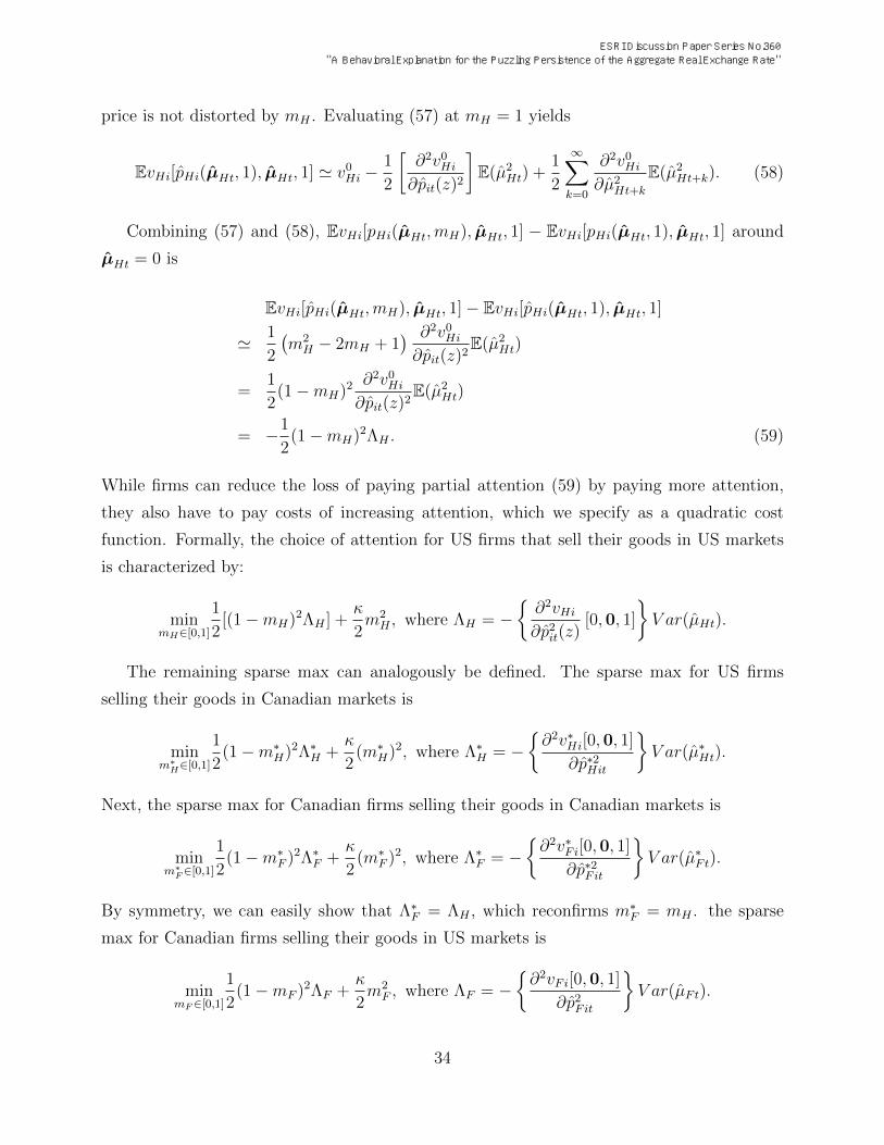
price is not distorted by mH . Evaluating (57) at mH = 1 yields

EvHi[pHi(µHt, 1), µHt, 1] ' v0Hi −1

2

[∂2v0Hi∂pit(z)2

]E(µ2

Ht) +1

2

∞∑k=0

∂2v0Hi∂µ2

Ht+k

E(µ2Ht+k). (58)

Combining (57) and (58), EvHi[pHi(µHt,mH), µHt, 1] − EvHi[pHi(µHt, 1), µHt, 1] around

µHt = 0 is

EvHi[pHi(µHt,mH), µHt, 1]− EvHi[pHi(µHt, 1), µHt, 1]

' 1

2

(m2H − 2mH + 1

) ∂2v0Hi∂pit(z)2

E(µ2Ht)

=1

2(1−mH)2

∂2v0Hi∂pit(z)2

E(µ2Ht)

= −1

2(1−mH)2ΛH . (59)

While firms can reduce the loss of paying partial attention (59) by paying more attention,

they also have to pay costs of increasing attention, which we specify as a quadratic cost

function. Formally, the choice of attention for US firms that sell their goods in US markets

is characterized by:

minmH∈[0,1]

1

2[(1−mH)2ΛH ] +

κ

2m2H , where ΛH = −

{∂2vHi∂p2it(z)

[0,0, 1]

}V ar(µHt).

The remaining sparse max can analogously be defined. The sparse max for US firms

selling their goods in Canadian markets is

minm∗

H∈[0,1]

1

2(1−m∗H)2Λ∗H +

κ

2(m∗H)2, where Λ∗H = −

{∂2v∗Hi[0,0, 1]

∂p∗2Hit

}V ar(µ∗Ht).

Next, the sparse max for Canadian firms selling their goods in Canadian markets is

minm∗

F∈[0,1]

1

2(1−m∗F )2Λ∗F +

κ

2(m∗F )2, where Λ∗F = −

{∂2v∗Fi[0,0, 1]

∂p∗2Fit

}V ar(µ∗Ft).

By symmetry, we can easily show that Λ∗F = ΛH , which reconfirms m∗F = mH . the sparse

max for Canadian firms selling their goods in US markets is

minmF∈[0,1]

1

2(1−mF )2ΛF +

κ

2m2F , where ΛF = −

{∂2vFi[0,0, 1]

∂p2Fit

}V ar(µFt).

34


Again, by symmetry, we have ΛF = Λ∗H and mF = m∗H .

A.3 The optimal prices under behavioral inattention

Using the definition of µHt+k, we rewrite the log-linearized first-order condition (19) as

pHi(µHt,mH) = (1−λδ)Et∞∑k=0

(λδ)k(mHwt+k− ait+k)+mH(1−λδ)Et∞∑k=0

(λδ)kk∑l=1

πt+l, (60)

where we used µHt+k = wt+k +∑k

l=1 πt+l.

We separately arrange the terms in the right-hand side of (60). First, note that

(1− λδ)Et∞∑k=0

(λδ)k(mHwt+k − ait+k)

= Et∞∑k=0

(λδ)k(mHwt+k − ait+k)− Et∞∑k=0

(λδ)k+1(mHwt+k − ait+k)

= mHwt − ait+Et[(λδ)1(mHwt+1 − ait+1)− (λδ)1(mHwt − ait)]

+Et[(λδ)2(mHwt+2 − ait+2)− (λδ)2(mHwt+1 − ait+1)]

+...

= mHwt − ait + Et∞∑k=1

(λδ)k(mH∆wt+k −∆ait+k).

Next, the remaining terms are

mH(1− λδ)Et∞∑k=0

(λδ)kk∑l=1

πt+l

= mH(1− λδ)Et

(λδ)πt+1

+(λδ)2πt+1 + (λδ)2πt+2

+(λδ)3πt+1 + (λδ)3πt+2 + (λδ)3πt+3+...

= mH(1− λδ)Et

{(λδ)

[∞∑k=0

(λδ)k

]πt+1 + (λδ)2

[∞∑k=0

(λδ)k

]πt+2 + (λδ)3

[∞∑k=0

(λδ)k

]πt+3 + ...

}

= mHEt∞∑k=1

(λδ)kπt+k,

where the last line uses∑∞

k=0(λδ)k = (1 − λδ)−1. Finally, combining the above expressions,

35


(60) becomes

pHi(µHt,mH) = (mHwt − ait) + Et∞∑k=1

(λδ)k{mH(∆wt+k + πt+k)−∆ait+k}. (61)

Now, under the assumption of U(c, n) = ln c − χnt, the first-order conditions of US

households (Wt/Pt = χct) imply wt = ct. In addition, their CIA constraint (Mt = Ptct) leads

to πt = lnMt/Mt−1 − ∆ct. Thus, using (15), we have ∆wt + πt = lnMt/Mt−1 = εMt . As a

result, (61) becomes

pHi(µHt,mH) = (mHwt − ait)− Et∞∑k=1

(λδ)k∆ait+k.

If the stochastic process ait is given by (17), Et∑∞

k=1(λδ)k∆ait+k = −λδait. Therefore,

pHi(µHt,mH) = mHwt − (1− λδ)ait,

which is (20) in the main text.

For the price of goods exported by US firms, we have

p∗Hi(µ∗Ht,m

∗H) = [m∗H(wt − qt)− ait] + Et

∞∑k=1

(λδ)k[mH(∆wt+k −∆qt+k + π∗t+k)−∆ait+k]

= (m∗Hw∗t − ait) + Et

∞∑k=1

(λδ)k[mH(∆w∗t+k + π∗t+k)−∆ait+k], (62)

where we used the log-linearized equation of (3): qt = ct − c∗t = wt − w∗t . This equation has

the same structure as (61). Using the CIA constraint, (16), and (17), the above equation can

be simplified to

p∗Hi(µ∗Ht,m

∗H) = m∗H(wt − qt)− (1− λδ)ait,

which is equivalent to (21).

The remaining optimal prices, namely p∗Fi(µ∗Ft,m

∗F ) and pFi(µFt,mF ) are analogously

derived.

36


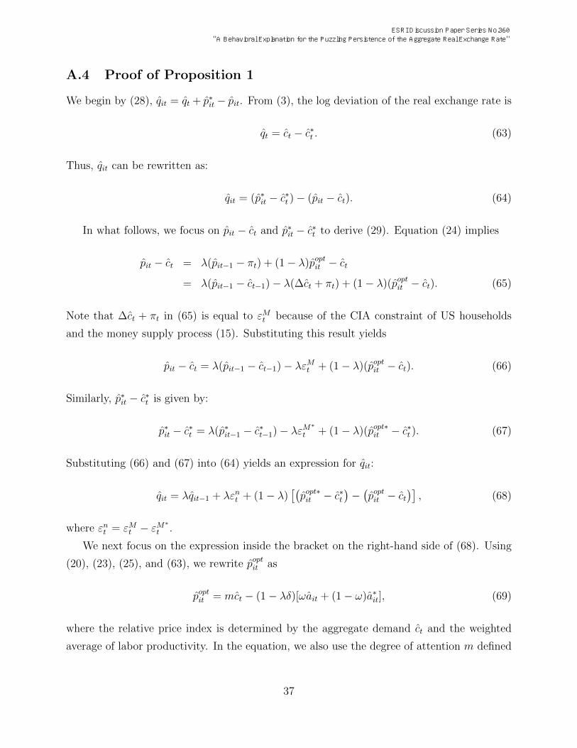
A.4 Proof of Proposition 1

We begin by (28), qit = qt + p∗it − pit. From (3), the log deviation of the real exchange rate is

qt = ct − c∗t . (63)

Thus, qit can be rewritten as:

qit = (p∗it − c∗t )− (pit − ct). (64)

In what follows, we focus on pit − ct and p∗it − c∗t to derive (29). Equation (24) implies

pit − ct = λ(pit−1 − πt) + (1− λ)poptit − ct= λ(pit−1 − ct−1)− λ(∆ct + πt) + (1− λ)(poptit − ct). (65)

Note that ∆ct + πt in (65) is equal to εMt because of the CIA constraint of US households

and the money supply process (15). Substituting this result yields

pit − ct = λ(pit−1 − ct−1)− λεMt + (1− λ)(poptit − ct). (66)

Similarly, p∗it − c∗t is given by:

p∗it − c∗t = λ(p∗it−1 − c∗t−1)− λεM∗

t + (1− λ)(popt∗it − c∗t ). (67)

Substituting (66) and (67) into (64) yields an expression for qit:

qit = λqit−1 + λεnt + (1− λ)[(popt∗it − c∗t

)−(poptit − ct

)], (68)

where εnt = εMt − εM∗

t .

We next focus on the expression inside the bracket on the right-hand side of (68). Using

(20), (23), (25), and (63), we rewrite poptit as

poptit = mct − (1− λδ)[ωait + (1− ω)a∗it], (69)

where the relative price index is determined by the aggregate demand ct and the weighted

average of labor productivity. In the equation, we also use the degree of attention m defined

37


by (30). We then subtract ct from both sides of (69) to get

poptit − ct = − (1−m) ct − (1− λδ) [ωait + (1− ω) a∗it] . (70)

Similarly, popt∗it − c∗t is

popt∗it − c∗t = −(1−m)c∗t − (1− λδ)[ωa∗it + (1− ω)ait], (71)

where m = ωm∗F + (1− ω)m∗H = ωmH + (1− ω)mF . Combining (70) and (71), we have

(popt∗it − c∗t )− (poptit − ct) = (1−m)(ct − c∗t ) + (1− λδ)(2ω − 1)(ait − a∗it)

= (1−m)qt + (1− λδ)ψεrit,

where qt = ct − c∗t from (63), εrit = εit − ε∗it = ait − a∗it from (17) and (18), and ψ = 2ω − 1.

Substituting the above equation into (68) yields

qit = λqit−1 + (1− λ) (1−m) qt + λεnt + (1− λ) (1− λδ)ψεrit. (72)

Here, qit = ln qit and qt = ln qt because ln qi = ln q = 0 from the symmetry between the

two countries. In particular, the symmetry ensures that ln q = ln c − ln c∗ = 0 and that

ln qi = ln q + p∗i − pi = 0. Therefore, (72) is equivalent to (29) in Proposition 1.

A.5 Estimation results for (40)

Table A.1 reports the estimation results for (40) by GMM. We report the results of four

specifications. In specifications (2) and (4), we impose the restriction that the coefficients

on ln qit−1 and ∆ lnSt as control variables are the same as each other. This is because (29)

indicates that ln qit−1 and εnt = ∆ lnSt have the same coefficient. Specifications (3) and (4)

differ from specifications (1) and (2) in that the regressions include ηrt as a control variable.

The table indicates that, in all regressions, the null hypothesis that β = 0 in (40) is

statistically rejected. In addition, the estimates of β are all positive, consistent with the

theory. Therefore, even if we directly regress ln qijt on ln qt, the data are consistent with the

partial attention of 0 < m < 1.

38


A.6 Persistence of the good-level real exchange rate

A.6.1 Proof of Proposition 3

As a preparation, we rewrite (41) in terms of the log deviation:

qt = ρq qt−1 + ρqεnt . (73)

The variance of qt is given by σ2q = [ρ2q/(1− ρ2q)]σ2

n, so

σ2n =

1− ρ2qρ2q

σ2q . (74)

In Appendix A.4, we have shown that the log deviation of the LOP deviations is

qit = λqit−1 + θqt + λεnt + ψεrit, (75)

where θ = (1− λ)(1−m) and ψ = (1− λ) (1− λδ)ψ.

Let the covariances denote R0 = Eqtqit and R1 = Eqtqit−1. They are written as

R0 = λR1 + θσ2q + λρqσ

2n, (76)

R1 = ρqR0, (77)

which can be derived from (73) and (75).

We further simplify (76) and (77). Substitute (74) and (77) into (76) to get

R0 = λρqR0 +

[θ +

λ(1− ρ2q)ρq

]σ2q . (78)

Note that, using the definition of ρq, the expression inside the brackets can be simplified as29

θ +λ(1− ρ2q)

ρq= 1− λρq. (79)

29To see this, θ+ λ(1− ρ2q)/ρq = θ+ λ(1− ρ2q)/(λ/(1− θ)) = θ+ (1− ρ2q)(1− θ) = 1− ρ2q(1− θ). Applyingthe definition of ρq to this equation again, we obtain (79).

39


Using (79), (78) and (77) become

R0 = σ2q , (80)

R1 = ρqσ2q , (81)

respectively.

We next work on the variance and the autocovariance that are denoted as σ2qi = Eq2it and

γ1 = Eqitqit−1, respectively. Using (75), (80), and (81), we have

σ2qi = λγ1 + θσ2

q + λρqσ2n + ψ2σ2

r , (82)

γ1 = λσ2qi + θρqσ

2q . (83)

We obtain (82) and (83) from tedious algebra. Regarding (82), we use (75) and (80)

σ2qi = Eq2it = λE(qitqit−1) + θE(qitqt) + λE(qitε

nt ) + ψE(qitε

rit)

= λγ1 + θσ2q + λE(qitε

nt ) + ψE(qitε

rit).

Simplifying the last two terms on the right-hand side of the above equation yields (82):


q + λE[(λqit−1 + θqt + λεnt + ψεrit)εnt ] + ψE[(λqit−1 + θqt + λεnt + ψεrit)ε

rit]

= λγ1 + θσ2q + λθE(qtε

nt ) + λ2σ2

n + ψ2σ2r

= λγ1 + θσ2q + λ(θρq + λ)σ2

n + ψ2σ2r

= λγ1 + θσ2q + λρqσ

2n + ψ2σ2

r .

The third equality results from (73), and the fourth equality is from the definition of ρq.

Regarding (83), use (75) and (81) to get

γ1 = Eqitqit−1 = λE(qit−1qit−1) + θE(qtqit−1) + λE(εnt qit−1) + ψE(εritqit−1) = λσ2qi + ρqθσ

2q .

40


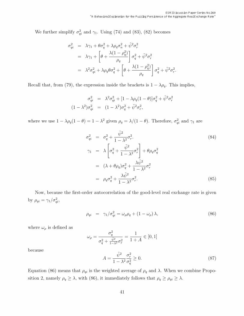
We further simplify σ2qi and γ1. Using (74) and (83), (82) becomes


q + λρqσ2n + ψ2σ2

r

= λγ1 +

[θ +

λ(1− ρ2q)ρq

]σ2q + ψ2σ2

r

= λ2σ2qi + λρqθσ

2q +

[θ +

λ(1− ρ2q)ρq

]σ2q + ψ2σ2

r .

Recall that, from (79), the expression inside the brackets is 1− λρq. This implies,

σ2qi = λ2σ2

qi + [1− λρq(1− θ)]σ2q + ψ2σ2

r

(1− λ2)σ2qi = (1− λ2)σ2

q + ψ2σ2r ,

where we use 1− λρq(1− θ) = 1− λ2 given ρq = λ/(1− θ). Therefore, σ2qi and γ1 are

σ2qi = σ2

q +ψ2

1− λ2σ2r . (84)

γ1 = λ

[σ2q +

ψ2

1− λ2σ2r

]+ θρqσ

2q

= (λ+ θρq)σ2q +

λψ2

1− λ2σ2r

= ρqσ2q +

λψ2

1− λ2σ2r . (85)

Now, because the first-order autocorrelation of the good-level real exchange rate is given

by ρqi = γ1/σ2qi,

ρqi = γ1/σ2qi = ωρρq + (1− ωρ)λ, (86)

where ωρ is defined as

ωρ =σ2q

σ2q + ψ2

1−λ2σ2r

=1

1 + A∈ [0, 1]

because

A =ψ2

1− λ2σ2r

σ2q

≥ 0. (87)

Equation (86) means that ρqi is the weighted average of ρq and λ. When we combine Propo-

sition 2, namely ρq ≥ λ, with (86), it immediately follows that ρq ≥ ρqi ≥ λ.

41


A.6.2 Derivation of (45) and (46)

Using ρq = λ/(1− θ), eliminate λ from (86):

ρqi = ωρρq + (1− ωρ) (1− θ) ρq = ρq [1− θ (1− ωρ)] . (88)

Recall (74) and the definition of ψ. Then, (87) becomes (46):

A = (1− λ)2(1− λδ)2ψ21− ρ2q

ρ2q(1− λ2)

(σrσn

)2

. (89)

From ωρ = 1/ (1 + A), 1 − ωρ = A/(1 + A). In addition, recall that θ = (1 − λ)(1 − m).

Therefore, (88) impliesρqρqi

=1

1− (1− λ) (1−m) A1+A

. (90)

A.7 The model with CRRA preferences

Let us assume more general CRRA preferences: U(c, n) = c1−σ/(1 − σ) − χn1+ϕ/(1 + ϕ).

We modify the first-order conditions for households to allow for the degree of relative risk

aversion. Under σ 6= 1, the first-order conditions imply St = (Mt/M∗t )σ(Pt/P

∗t )1−σ.

If we maintain the assumption that the money supply follows a random walk, the equation

for St leads to the nominal exchange rate growth that is predictable through the inflation of

the two countries.30 Because this is inconsistent with the exchange-rate disconnect puzzle,

we replace this assumption by the new assumption on the money growth rate:

∆ lnMt =σ − 1

σπt +

1

σεMt , (91)

∆ lnM∗t =

σ − 1

σπ∗t +

1

σεM

∗

t . (92)

Under (91) and (92), the nominal exchange rate continues to follow a random walk.31

30In particular, the nominal exchange rate growth is given by ∆st = σεnt + (1− σ)(πt − π∗t ), meaning that

πt − π∗t can help forecast ∆st.

31To see this, note that the nominal exchange rate growth is given by: ∆st = σ (∆ lnMt −∆ lnM∗t ) +

(1− σ) (πt − π∗t ). Substituting (91) and (92) into the above equation yields ∆st = (σ − 1) (πt − π∗

t ) +(1− σ) (πt − π∗

t ) + εMt − εM∗

t = εnt .

42


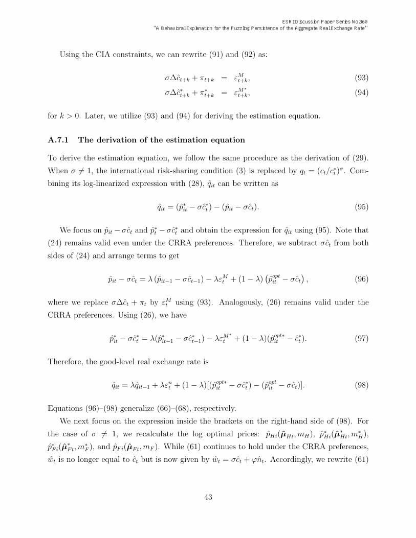
Using the CIA constraints, we can rewrite (91) and (92) as:

σ∆ct+k + πt+k = εMt+k, (93)

σ∆c∗t+k + π∗t+k = εM∗

t+k, (94)

for k > 0. Later, we utilize (93) and (94) for deriving the estimation equation.

A.7.1 The derivation of the estimation equation

To derive the estimation equation, we follow the same procedure as the derivation of (29).

When σ 6= 1, the international risk-sharing condition (3) is replaced by qt = (ct/c∗t )σ. Com-

bining its log-linearized expression with (28), qit can be written as

qit = (p∗it − σc∗t )− (pit − σct). (95)

We focus on pit− σct and p∗t − σc∗t and obtain the expression for qit using (95). Note that

(24) remains valid even under the CRRA preferences. Therefore, we subtract σct from both

sides of (24) and arrange terms to get

pit − σct = λ (pit−1 − σct−1)− λεMt + (1− λ)(poptit − σct

), (96)

where we replace σ∆ct + πt by εMt using (93). Analogously, (26) remains valid under the

CRRA preferences. Using (26), we have

p∗it − σc∗t = λ(p∗it−1 − σc∗t−1)− λεM∗

t + (1− λ)(popt∗it − c∗t ). (97)

Therefore, the good-level real exchange rate is

qit = λqit−1 + λεnt + (1− λ)[(popt∗it − σc∗t )− (poptit − σct)]. (98)

Equations (96)–(98) generalize (66)–(68), respectively.

We next focus on the expression inside the brackets on the right-hand side of (98). For

the case of σ 6= 1, we recalculate the log optimal prices: pHi(µHt,mH), p∗Hi(µ∗Ht,m

∗H),

p∗Fi(µ∗Ft,m

∗F ), and pFi(µFt,mF ). While (61) continues to hold under the CRRA preferences,

wt is no longer equal to ct but is now given by wt = σct + ϕnt. Accordingly, we rewrite (61)

43


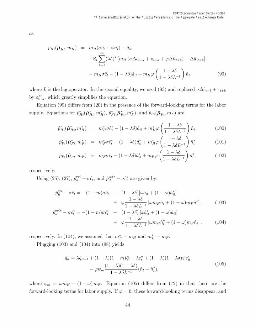
as

pHi(µHt,mH) = mH(σct + ϕnt)− ait

+Et∞∑k=1

(λδ)k [mH (σ∆ct+k + πt+k + ϕ∆nt+k)−∆ait+k] .

= mHσct − (1− λδ)ait +mHϕ

(1− λδ

1− λδL−1

)nt. (99)

where L is the lag operator. In the second equality, we used (93) and replaced σ∆ct+k + πt+k

by εMt+k, which greatly simplifies the equation.

Equation (99) differs from (20) in the presence of the forward-looking terms for the labor

supply. Equations for p∗Hi(µ∗Ht,m

∗H), p∗Fi(µ

∗Ft,m

∗F ), and pFi(µFt,mF ) are

p∗Hi(µ∗Ht,m

∗H) = m∗Hσc

∗t − (1− λδ)ait +m∗Hϕ

(1− λδ

1− λδL−1

)nt, (100)

p∗Fi(µ∗Ft,m

∗F ) = m∗Fσc

∗t − (1− λδ)a∗it +m∗Hϕ

(1− λδ

1− λδL−1

)n∗t , (101)

pFi(µFt,mF ) = mFσct − (1− λδ)a∗it +mFϕ

(1− λδ

1− λδL−1

)n∗t , (102)

respectively.

Using (25), (27), poptit − σct, and popt∗it − σc∗t are given by:

poptit − σct = −(1−m)σct − (1− λδ)[ωait + (1− ω)a∗it]

+ ϕ1− λδ

1− λδL−1[ωmH nt + (1− ω)mF n

∗t ] , (103)

popt∗it − σc∗t = −(1−m)σc∗t − (1− λδ) [ωa∗it + (1− ω)ait]

+ ϕ1− λδ

1− λδL−1[ωmH n

∗t + (1− ω)mF nt] , (104)

respectively. In (104), we assumed that m∗F = mH and m∗H = mF .

Plugging (103) and (104) into (98) yields

qit = λqit−1 + (1− λ)(1−m)qt + λεnt + (1− λ)(1− λδ)ψεrit

− ϕψm(1− λ)(1− λδ)

1− λδL−1(nt − n∗t ),

(105)

where ψm = ωmH − (1− ω)mF . Equation (105) differs from (72) in that there are the

forward-looking terms for labor supply. If ϕ = 0, these forward-looking terms disappear, and

44


the equation coincides with (72). Under our assumptions, σ does not appear in (105). More

importantly, σ does not affect the coefficient on the aggregate real exchange rate.

As in the proof of Proposition 2, the symmetry between the two countries implies that

qi = q = 1, and thus qit = ln qit and qt = ln qt. Likewise, the symmetry implies the same

steady-state labor supply between the two countries: n = n∗, leading to nt−n∗t = lnnt−lnn∗t .

Substitution of these equations into the above equation leads to

ln qit = λ ln qit−1 + (1− λ)(1−m) ln qt + λεnt + (1− λ)(1− λδ)ψεrit (106)

−ϕψm(1− λ)(1− λδ)

1− λδL−1(lnnt − lnn∗t ) ,

which generalizes (29).

To derive the estimation equation for our empirical analysis, we use the definition of qit

and qt and further rewrite (106) as

ln qit = (1−m) ln qt + (1− λ)(1− λδ)ψεrit − ϕψm(1− λ)(1− λδ)

1− λδL−1(lnnt − lnn∗t ),

or equivalently,

ln qit − λδEt ln qit+1 = (1−m)(ln qt − λδEt ln qt+1) (107)

−(1− λ)(1− λδ)ϕψm(lnnt − lnn∗t ) + (1− λ)(1− λδ)ψεrit,

where Etεrit+1 = 0.

Let ln ˜qit = ln qit − λδqit+1 and ln ˜qt = qt − λδqt+1. Our estimation equation is

ln ˜qit = α + β ln ˜qt + γ′Xit + uit, (108)

where Xit includes the log-difference in labor supply lnnt− lnn∗t and γ includes −(1−λ)(1−λδ)ϕψm as an element. Note that OLS is no longer a valid estimation because uit now

includes forecast error ln qit+1−Et ln qit+1 and ln qt+1−Et ln qt+1. We thus use the instrument

for estimation. For the data source of lnnt − lnn∗t , we take the indices of total hours worked

from OECD.Stat with the base year 2010.

Table A.2 reports the estimation results based on (108). We use a common λ in speci-

fications (1) and (2) and the good-specific λ in specifications (3) and (4). In addition, we

instrument ln ˜qt by ln qt−1 in specifications (1) and (3) and ln ˜qt−1 in specifications (2) and

45


(4). In all cases, the null hypothesis of full attention, namely β = 0, is significantly rejected.

The estimated values of m are also very close to each other, suggesting robustness to changes

in the assumption of preferences.

46


Figure 1: Empirical distributions of the good-level real exchange rates

0.2

.4.6

.81

density

−2 −1 0 1 2the log of good−level real exchange rate

1990 2015

47


Figure 2: Persistence of the aggregate real exchange rate and the ρq to λ ratio

0 0.2 0.4 0.6 0.8 1

m

0

0.1

0.2

0.3

0.4

0.5

0.6

0.7

0.8

0.9

1

q

q with = 0.34

q with = 0.68

0 0.2 0.4 0.6 0.8 1

m

1

1.2

1.4

1.6

1.8

2

2.2

2.4

2.6

2.8

3

q/

q/ with = 0.34

q/ with = 0.68

q/ = 1

Figure 3: Persistence of the aggregate and the good-level real exchange rates and the ρq toρqi ratio

0 0.2 0.4 0.6 0.8 1

m

0

0.1

0.2

0.3

0.4

0.5

0.6

0.7

0.8

0.9

1

q,

qi,

q

qi

=0.34

0 0.2 0.4 0.6 0.8 1

m

0.9

1

1.1

1.2

1.3

1.4

1.5

1.6

1.7

q/

qi

q/

qi

q/

qi = 1

48


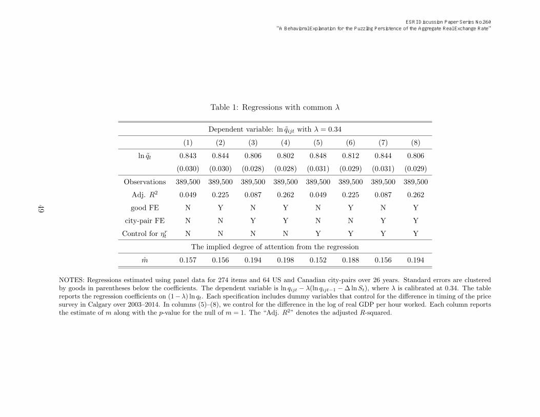
Table 1: Regressions with common λ

Dependent variable: ln qijt with λ = 0.34

(1) (2) (3) (4) (5) (6) (7) (8)

ln qt 0.843 0.844 0.806 0.802 0.848 0.812 0.844 0.806

(0.030) (0.030) (0.028) (0.028) (0.031) (0.029) (0.031) (0.029)

Observations 389,500 389,500 389,500 389,500 389,500 389,500 389,500 389,500

Adj. R2 0.049 0.225 0.087 0.262 0.049 0.225 0.087 0.262

good FE N Y N Y N Y N Y

city-pair FE N N Y Y N N Y Y

Control for ηrt N N N N Y Y Y Y

The implied degree of attention from the regression

m 0.157 0.156 0.194 0.198 0.152 0.188 0.156 0.194

NOTES: Regressions estimated using panel data for 274 items and 64 US and Canadian city-pairs over 26 years. Standard errors are clusteredby goods in parentheses below the coefficients. The dependent variable is ln qijt − λ(ln qijt−1 − ∆ lnSt), where λ is calibrated at 0.34. The tablereports the regression coefficients on (1−λ) ln qt. Each specification includes dummy variables that control for the difference in timing of the pricesurvey in Calgary over 2003–2014. In columns (5)–(8), we control for the difference in the log of real GDP per hour worked. Each column reportsthe estimate of m along with the p-value for the null of m = 1. The “Adj. R2” denotes the adjusted R-squared.

49


Table 2: Regressions with good-specific λ

Dependent variable: ln qijt with good-specific λ

(1) (2) (3) (4) (5) (6) (7) (8)

ln qt 0.793 0.894 0.766 0.862 0.765 0.883 0.763 0.88

(0.045) (0.029) (0.045) (0.028) (0.053) (0.032) (0.053) (0.033)

Observations 389,500 389,500 389,500 389,500 389,500 389,500 389,500 389,500

Adj. R2 0.062 0.256 0.100 0.294 0.062 0.256 0.100 0.294

good FE N Y N Y N Y N Y

city-pair FE N N Y Y N N Y Y

Control for ηrt N N N N Y Y Y Y


m 0.207 0.106 0.234 0.138 0.235 0.117 0.237 0.120

NOTES: The dependent variable is ln qijt = ln qijt − λi[ln qijt−1 − ln(St/St−1)], where λi is good specific and calibrated based on Nakamura and

Steinsson (2008). The table reports the regression coefficients on ln qit = ln(qt/qλit ). See the notes to Table 1 for the remaining details.

50


Table 3: Persistence implied by the estimated degree of attention

Model with Model with behavioral inattention Data

full attention m = 0.237 m = 0.174 m = 0.106

The aggregate real exchange rate

HL 0.643 1.831 2.382 3.704 3-5

ρq 0.340 0.685 0.748 0.829 0.79-0.87

The good-level real exchange rate

HL 0.643 0.819 0.933 1.223 1.0-1.6

ρqi 0.340 0.429 0.476 0.567 0.51-0.65

NOTES: The table reports the half-lives (denoted “HL”) and the first-order autocorrelations (denoted ρqand ρqi) of the real exchange rates predicted by the model. The unit of half-lives is a year. To calculatethe predicted values in the table, we use the calibrated values of λ = 0.34, τ = 0.74, ε = 4, σr/σ∆s = 5,and δ = 0.98. The computed persistence measures are based on m = 0.237 (the largest estimate in Tables 1and 2), m = 0.174 (the mean of the estimates in Tables 1 and 2), and m = 0.106 (the smallest estimate inTables 1 and 2), together with the model with full attention (m = 1) for reference. The rightmost columnreports estimates from previous studies for comparison. For the aggregate real exchange rate, we take therange of the half-lives from Rogoff (1996) and compute the implied first-order autocorrelations from the half-lives. For the good-level real exchange rate, we take the median estimate of the half-lives and the first-orderautocorrelations of all goods provided in Table 4 of Crucini and Shintani (2008).

51


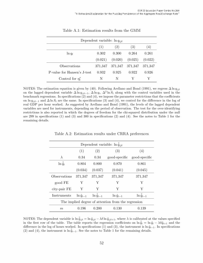
Table A.1: Estimation results from the GMM

Dependent variable: ln qijt

(1) (2) (3) (4)

ln qt 0.302 0.300 0.264 0.261

(0.021) (0.020) (0.025) (0.022)

Observations 371,347 371,347 371,347 371,347

P-value for Hansen’s J-test 0.932 0.925 0.922 0.926

Control for ηrt N N Y Y

NOTES: The estimation equation is given by (40). Following Arellano and Bond (1991), we regress ∆ ln qijton the lagged dependent variable ∆ ln qijt−1, ∆ ln qt, ∆2 lnSt along with the control variables used in thebenchmark regressions. In specifications (2) and (4), we impose the parameter restrictions that the coefficientson ln qijt−1 and ∆ lnSt are the same. In specifications (3) and (4), we control for the difference in the log ofreal GDP per hour worked. As suggested by Arellano and Bond (1991), the levels of the lagged dependentvariables are used for instruments, depending on the period of observation. The test for the over-identifyingrestrictions is also reported in which the degrees of freedom for the chi-squared distribution under the nullare 299 in specifications (1) and (3) and 300 in specifications (2) and (4). See the notes to Table 1 for theremaining details.

Table A.2: Estimation results under CRRA preferences

Dependent variable: ln ˜qijt

(1) (2) (3) (4)

λ 0.34 0.34 good-specific good-specific

ln ˜qt 0.804 0.800 0.870 0.861

(0.034) (0.037) (0.041) (0.045)

Observations 371,347 371,347 371,347 371,347

good FE Y Y Y Y

city-pair FE Y Y Y Y

Instruments ln qt−1 ln ˜qt−1 ln qt−1 ln ˜qt−1


m 0.196 0.200 0.130 0.139

NOTES: The dependent variable is ln ˜qijt = ln qijt − λδ ln qijt+1, where λ is calibrated at the values specifiedin the first row of the table. The table reports the regression coefficients on ln ˜qt = ln qt − λδqt+1 and thedifference in the log of hours worked. In specifications (1) and (3), the instrument is ln qt−1. In specifications(2) and (4), the instrument is ln ˜qt−1. See the notes to Table 1 for the remaining details.

52


Documents

A Behavioral Explanation for the Puzzling Persistence of