A Bayesian Approach to Diameter Estimation in the Diameter Control System of Silicon Single Crystal Growth

IEEE TRANSACTIONS ON INSTRUMENTATION AND MEASUREMENT, VOL. 60, NO. 4, APRIL 2011 1307

A Bayesian Approach to Diameter Estimation inthe Diameter Control System of Silicon

Single Crystal GrowthDing Liu, Member, IEEE, and Junli Liang

Abstract—In the diameter control system of silicon single crystalgrowth, the variation of the diameter of the aperture (i.e., a halowith high brightness, which appears at the junction of a solidcrystal and a liquid solution) is consistent with the change in thediameter of the growing crystal. Therefore, the diameter of theaperture can be used as a control variable for adjusting the castingspeed and temperature so that the grown silicon single crystalapproximates to a perfect cylinder. It is obvious that the measureddiameter of the current aperture plays an important role in thediameter control system of silicon single crystal growth. In fact,the obtained aperture image from a charge-coupled device camerais a halo of ellipses instead of circles. To estimate the diameter(or radius) of the elliptical aperture, we propose a Bayesian ap-proach, in which a Bayesian model is derived to define a posteriordistribution for the unknown parameters. This distribution istoo complicated for analytical extraction of moments to sampledirectly. An efficient computational algorithm based on a Markovchain Monte Carlo method is derived to estimate the posteriordistribution and draw samples from the distribution. Comparingwith the classical Hough transform-based algorithm and the directleast-squares fitting method, the proposed algorithm has higherestimation accuracy. Some simulated and experimental examplesare presented to illustrate the algorithm’s effectiveness.

Index Terms—Bayesian inference, diameter estimation, ellipsefitting, growth control, silicon single crystal.

I. INTRODUCTION

AUTOMATIC interpretation, acquisition, and measure-ment of the information of product features is an im-

portant procedure in automated manufacturing systems, suchas automobile body assembly [1], manufacturing automation[2], computer-aided manufacturing [3], computer-aided designmodel construction [4], vision-based inspection system [5],

Manuscript received December 3, 2009; revised April 26, 2010; acceptedJune 5, 2010. Date of publication November 9, 2010; date of current versionMarch 8, 2011. This work was supported by the Important National Scienceand Technology Specific Project under Grant 2009x02011001, by the NationalNatural Science Foundations of China under Grant 60901059 and 61075044,by the third special postdoctoral science foundation of China under Grant201003679, by the Educational Department Foundation Grant 09JK629 andNatural Science Foundation under Grant 2010JQ8001 of Shaanxi Province,and by the Discipline Union Fund under Grant 116-210905 and the DoctorResearch Start Fund under Grant 116-210903 of Xi’an University of Technol-ogy. The Associate Editor coordinating the review process for this paper wasDr. Antonios Tsourdos.

The authors are with the School of Automation and Information Engineering,Xi’an University of Technology, Xi’an 710048, China (e-mail: [email protected]).

Color versions of one or more of the figures in this paper are available onlineat http://ieeexplore.ieee.org.

Digital Object Identifier 10.1109/TIM.2010.2086610

and welding economic design [6]. With the increasing demandfor manufacturing automation, curve fitting, particularly ellipsefitting, receives considerable attention because it plays a keyrole in crystal growth control [7], computer vision [8]–[10],observational astronomy, structural geology, reverse engineer-ing, rapid prototyping, etc. In the diameter control system ofsilicon single crystal growth [11], the control of the crystaldiameter is a key step to ensure that the crystal always growswith equivalent diameter [12]. To prevent the crystal diameterfrom getting thicker due to the acceleration of crystallization,one can improve the seed crystal and increase the temperature[13]. On the other hand, one can reduce the speed and decreasethe temperature to prevent the crystal diameter from gettingthinner due to the slowness of crystallization. In the processof crystallization, an aperture (a halo with high brightness,which results from the fact that the meniscus at the solid–liquidinterfaces reflects the lights of the crucible wall) will appear atthe junction of a solid crystal and a liquid solution. The vari-ation of the measured aperture diameter is consistent with thechange of the real diameter of the growing crystal. In this case,detecting the varying trends of the aperture is actually findingthe changing trends of the crystal diameter, and the diame-ter estimation problem from the image of the charge-coupleddevice (CCD) camera becomes an ellipse-fitting question.

The fitting problem can be viewed as follows: Given a setof points in a plane, estimate the parameters of the ellipse that“best fit” the data points. The algorithms to fit ellipses aregenerally classified into two categories: 1) the clustering-liketechniques (such as the Hough transform with expensive com-putation [14]) and 2) the least-squares (LS) methods [15]–[17].The latter ones attempt to find the parameters of an ellipse byminimizing an error metric between the primitive and the datapoints. Various LS fitting approaches fall into two categories:1) geometric methods, which are based on the orthogonaldistances between the data points and the estimated ellipse,must solve a nonlinear problem by iterative procedures [18];and 2) algebraic methods, which are extensively used due totheir linear nature simplicity and computational efficiency [19],[20]. A major advance in algebraic methods is direct LS fitting(DLSF) of ellipses proposed in [15]. Its primary contribution isa new constraint that guarantees that the optimum solution is anellipse while maintaining computational efficiency. Accordingto [16], the algebraic methods inherit high curvature bias andsensitivity to outliers. Recently, Barwick has proposed a chordmethod [16] that provides an indirect geometric fit based on the

0018-9456/$26.00 © 2010 IEEE

1308 IEEE TRANSACTIONS ON INSTRUMENTATION AND MEASUREMENT, VOL. 60, NO. 4, APRIL 2011

Fig. 1. CCD camera system for obtaining the aperture image.

quadratic polynomial form of parallel chord lengths. However,the chord approach heavily depends on the rigorous conditionthat the parallel chords perpendicular to a common axis must becollected. Once the condition is not satisfied, the chord methodwill not work.

In this paper, we propose a Bayesian approach to fit ellipsesand accordingly estimate the horizontal diameter (or radius) ofthe growing silicon single crystal. First, we derive a Bayesianmodel for fitting ellipses that allows us to define a posteriordistribution for the unknown ellipse center and axis lengths.Second, a Markov chain Monte Carlo (MCMC) [21]–[23]-based algorithm is derived to estimate the posterior distributionand draw samples from the distribution [24]. Finally, the sam-ples after an initial burn-in period are averaged as the parameterestimations.

The rest of this paper is organized as follows: The ellipsemodel used in this paper is introduced in Section II. A Bayesianapproach to ellipse fitting and radius (or diameter) estimation isdeveloped in Section III. Simulated and experimental results arepresented in Section IV. Conclusions are drawn in Section V.

II. PROBLEM FORMULATION

The equation for a general orientation ellipse centered at(h, k) with a counterclockwise rotation of θ and semiaxes (a, b)in x, y coordinates has the following form:

((x − h) cos θ + (y − k) sin θ)2

a2

+(−(x − h) sin θ + (y − k) cos θ)2

b2= 1. (1)

In the diameter control system of silicon single crystalgrowth, the aperture diameter is not directly detected in thecrystal furnace due to high temperature but detected from theimage of a CCD camera across the viewing window outsidethe pull-crystal furnace, as shown in Fig. 1. Since both the

Fig. 2. Related idea for the approximated Gaussian noise assumption.

base of the CCD camera and the aperture at the solid–liquidinterfaces are horizontal, and the camera is not just above theaperture, the aperture in the image is a halo of ellipses withthe counterclockwise rotation angle θ = 0◦, instead of circles.Therefore, the corresponding ellipse model can be simplified asthe following form:

(x − h)2

a2+

(y − k)2

b2= 1. (2)

After segmentation and edge detection of the image of thehigh-brightness aperture, some points (xi, yi), i = 1, · · · , I , areobtained, where I is the total number of data points. In theideal case, all these points are just on the ellipse since theyare the edge points of the aperture in the image, i.e., ((xi −h)2/a2) + ((yi − k)2/b2) = 1. However, since in the actualapplication, these points, which were obtained using imagesegmentation and edge detection operations, are not completelyprecise, some errors are introduced. Therefore, these points donot lie just on the ellipse but approximately scatter around theellipse, i.e., most of these points are on the ellipse, and somelie slightly inside (i.e., ((xi − h)2/a2) + ((yi − k)2/b2) < 1)or slightly outside the ellipse (i.e., ((xi − h)2/a2) + ((yi −k)2/b2) > 1). In other words, the pixels just on the true edgeof the aperture image are most likely selected as the aforemen-tioned data points, but the pixels, being far from the true edge,are chosen as the data points with a lower probability. Thus,((xi − h)2/a2) + ((yi − k)2/b2) obtained from the ith pointcan be viewed as a low-variance Gaussian noise disturbanceon 1 (the likelihood analyses and the central limit theorem[25], a large number of sample points), i.e., ((xi − h)2/a2) +((yi − k)2/b2) − 1 belongs to the Gaussian distribution. Theaforementioned idea can be illustrated in Fig. 2. In this figure,the red line represents the true ellipse, and the green line standsfor the approximated Gaussian probability density function.Based on the aforementioned idea, we introduce the followingequation:

(xi − h)2

a2+

(yi − k)2

b2− 1 = ni (3)

where ni is the zero-mean white Gaussian of low-variance σ2.The objective of this paper is to estimate the length a of the

semimajor axis and the parameters (b, h, k) from given edgepoints (xi, yi), i = 1, . . . , I . Since the horizontal radius of the

LIU AND LIANG: DIAMETER CONTROL SYSTEM OF SILICON SINGLE CRYSTAL GROWTH 1309

Fig. 3. Graph illustrating the hierarchical structure for the prior distributionsof the parameters (h, k, a, b, σ2).

growing silicon single crystal is one of the ellipse parameters,the ellipse-fitting algorithm can be used for estimating thehorizontal radius (or diameter).

III. PROPOSED ALGORITHM

Here, we follow a Bayesian approach [21]–[23] to fit anellipse and estimate the length a of the semimajor axis andthe parameters (b, h, k), which are sampled from appropriateprior distributions reflecting our degree of belief of the relevantvalues of the parameters.

Let x = [x1, x2, . . . , xI ] and y = [y1, y2, . . . , yI ]; thus, thelikelihood function from (3) is given by

p(x,y|h, k, a, b, σ2)

=I∏

i=1

1√2πσ2

exp

(− 1

2σ2

((xi−h)2

a2+

(yi−k)2

b2−1)2)

=(2πσ2)−I/2exp

(− 1

2σ2

I∑i=1

((xi−h)2

a2+

(yi−k)2

b2−1)2)

.

(4)

The Bayesian approach to ellipse fitting involves calculatingthe posterior distribution of the parameters (a, b, h, k). FromBayes’ theorem, the posterior distribution can be given by

p(h, k, a, b, σ2|x,y) ∝ p(x,y|h, k, a, b, σ2)p(h, k, a, b, σ2)(5)

where p(h, k, a, b, σ2) is the prior distribution for the parame-ters (h, k, a, b, σ2).

A. Prior Distributions

Here, we propose a hierarchical structure for the prior distri-butions of the parameters (h, k, a, b, σ2), which is illustrated bya directed acyclic graph, as shown in Fig. 3.

In Fig. 3, the random variables are shown by circular boxes,the fixed parameters by square boxes, and the data by a rec-tangular box. The actual forms of the prior distributions aregenerally chosen to be uninformative and conjugate. The useof conjugate priors allows some of the unknown parametersto be analytically integrated out, easing the computational

burden. For the variance σ2 of zero-mean white Gaussian noiseni, a conjugate inverse-Gamma prior distribution shown asσ2 ∼ 1/Ga(ν0, γ0) is assumed, where the introduced two extrahyperparameters ν0 and γ0 are small constants [24], i.e.,

p(σ2) = (γ0/2)ν0/2(σ2)−(ν0/2+1) exp(− γ0

2σ2

)/Γ(γ0

2

).

(6)

When ν0 = 0 and γ0 = 0, we obtain Jeffrey’s uninformativeprior p(σ2) ∝ 1/σ2 [24], which leads to a degenerate solu-tion. Therefore, the degenerate solution can be avoided byassigning an inverse-Gamma prior on the noise variance, whichalso offers the advantage of being a conjugate prior. Fouruninformative priors are assumed for a, b, h, and k, whichare independently uniformly distributed on a ∈ (amin, amax),b ∈ (bmin, bmax), h ∈ (hmin, hmax), and k ∈ (kmin, kmax),respectively.

The defined individual prior distributions are combined togive the following overall prior distribution:

p(h, k, a, b, σ2)∝ p(h)p(k)p(a)p(b)p(σ2)

=1

hmax−hmin× 1

kmax−kmin× 1

bmax−bmin

× 1amax−amin

×(γ0/2)ν0/2(σ2)−(ν0/2+1)

×exp(− γ0

2σ2

)/Γ(γ0

2

). (7)

B. Posterior Distributions

Applying (4) and (7) to (5), we have the following posteriordistribution:

p(h, k, a, b, σ2|x,y)

∝p(x,y|h, k, a, b, σ2)p(h)p(k)p(a)p(b)p(σ2)

=(2πσ2)−I/2exp

(− 1

2σ2

I∑i=1

((xi−h)2

a2+

(yi−k)2

b2−1)2)

× 1hmax−hmin

× 1kmax−kmin

× 1bmax−bmin

× 1amax−amin

×(γ0/2)ν0/2(σ2)−(ν0/2+1) exp(− γ0

2σ2

)/Γ(γ0

2

)ν0/2

∝(2πσ2)−I/2exp

(− 1

2σ2

I∑i=1

((xi−h)2

a2+

(yi−k)2

b2−1)2)

×(γ0/2)ν0/2(σ2)−(ν0/2+1) exp(− γ0

2σ2

)/Γ(γ0

2

)∝(σ2)−((ν0+I)/2+1)

×exp

⎛⎜⎜⎝−

γ0+I∑

i=1

((xi−h)2

a2 + (yi−k)2

b2 −1)2

2σ2

⎞⎟⎟⎠ . (8)


From (8), we can obtain the following conditional distribu-tion for σ2:

σ2|x,y, h, k, a, b ∼ Ga

(ν0 + I

2, z(h, k, a, b)

)(9)

where

Z(h, k, a, b) =I∑

i=1

((xi − h)2

a2+

(yi − k)2

b2− 1)2

. (10)

Therefore, we can reduce the complexity of the posterior distri-bution given in (8) by integrating out σ2. The resultant posteriordistribution can be given by

p(h, k, a, b|x,y) ∝ (γ0 + z(h, k, a, b))−12 (I+ν0) . (11)

We are unable to analytically integrate out other parameters(a, b, h, k); thus, the analytical methods cannot be used tocalculate the statistics of interest for this distribution. However,we can use a stochastic algorithm to sample from the jointposterior distribution p(h, k, a, b|x,y). From these samples, wecan obtain the estimation of these unknown parameters.

C. Sample From the Joint Posterior Distribution

The Bayesian inference of (a, b, h, k) is based on thejoint posterior distribution p(h, k, a, b|x,y) obtained fromBayes’ theorem. However, it requires the evaluation of high-dimensional integrals of nonlinear functions. Here, we use anMCMC method to perform Bayesian computation. MCMCtechniques were introduced in mid-1950s in statistical physicsbut have only been introduced in applied statistics in early1990s [21]–[23]. The key idea is to build an ergodic Markovchain, whose equilibrium distribution is the desired posteriordistribution. The Metropolis–Hastings (MH) algorithm candraw a sequence of random samples from a probability distrib-ution of a single random variable for which direct sampling isdifficult, whereas Gibbs sampling is an algorithm to generatea sequence of samples from the joint probability distributionof two or more random variables [24]. Here, we combineGibbs and MH steps to implement MCMC sampling: split theparameters (a, b, h, k) into four groups, then sample each one inturn from the conditional distribution, i.e., Gibbs sampler. Foreach unknown parameter, we implement a mixture of MH steps.

We implement similar MH steps for four unknown parame-ters a, b, h, and k. In the following description, we take a as anexample.

Let λ be a real number satisfying 0 < λ < 1. With a prob-ability λ, we perform an MH step with a proposal distributionqa,1(a′|a) independent of the current state a, which is assumedto be a uniform distribution, i.e., a′|a ∼ U(amin, amax). Themotivation for using such a proposal distribution is that theregions of interest of the posterior distribution are quicklyreached. The acceptance probability is given as follows:

min

{1,

(γ0 + z(h, k, a′, b))−12 (I+ν0) qa,1(a|a′)

(γ0 + z(h, k, a, b))−12 (I+ν0) qa,1(a′|a)

}. (12)

With a probability 1 − λ, we perform an MH step withproposal distribution qa,2(a′|a), which is assumed to be aGaussian distribution, i.e., a′|a ∼ N(a, σ2

RW). The proposaldistribution yields a candidate that is a perturbation a′ − a ofthe current value a. The perturbation is a zero-mean Gaussianrandom variable with variance σ2

RW. We perform this randomwalk to locally explore the posterior distribution and to ensureirreducibility of the Markov Chain. The acceptance probabilityfor the proposal distribution qa,2(a′|a) is given as follows:

min

{1,

(γ0 + z(h, k, a′, b))−12 (I+ν0) qa,2(a|a′)

(γ0 + z(h, k, a, b))−12 (I+ν0) qa,2(a′|a)

}. (13)

Similar to a, we implement the MH step for the un-known parameter b. With probabilities λ and 1 − λ, the pro-posal distributions b′|b ∼ U(bmin, bmax) and b′|b ∼ N(b, σ2

RW)are used, respectively. The related acceptance probabili-ties are similar to (12) and (13), except that symbolsz(h, k, a′, b), qa,1(a|a′), qa,1(a′|a), qa,2(a|a′), and qa,2(a′|a)are replaced with z(h, k, a, b′), qa,1(b|b′), qa,1(b′|b), qa,2(b|b′),and qa,2(b′|b), respectively.

Similar MH steps are implemented for the unknown parame-ters h and k.

D. Description of the Proposed Algorithm and the CompleteDiameter Estimation Procedure

Based on Section III-A–C, the proposed algorithm can bedescribed as follows:

Proposed Algorithm for Ellipse Fitting and DiameterEstimation:

1. Initialization. Set θ(0) = (h(0), k(0), a(0), b(0))2. Iteration i,

a) Sample u from the uniform distribution on [0, 1]. Ifu < λ, then execute an MH sampling step with a pro-posal distribution qa,1(a′|a(i)) and accept a(i+1)=a′

with the probability given in (12); Else, execute an MHsampling step with a proposal distribution qa,2(a′|a(i))and accept a(i+1)=a′ with the probability given in (13);

b) Similar to a), execute an MH sampling step for b;c) Similar to a), execute an MH sampling step for h;d) Similar to a), execute an MH sampling step for k;

3. 2 ∗ a is the horizontal diameter estimate in the currentiteration;

4. i = i + 1, go to step 2.

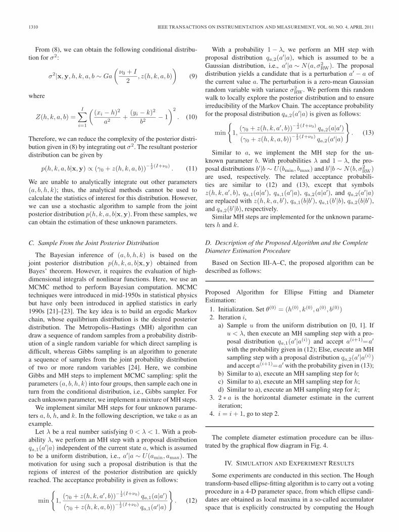
The complete diameter estimation procedure can be illus-trated by the graphical flow diagram in Fig. 4.

IV. SIMULATION AND EXPERIMENT RESULTS

Some experiments are conducted in this section. The Houghtransform-based ellipse-fitting algorithm is to carry out a votingprocedure in a 4-D parameter space, from which ellipse candi-dates are obtained as local maxima in a so-called accumulatorspace that is explicitly constructed by computing the Hough


Fig. 4. Graphical flow diagram for the diameter estimation system.

transform [14]. The DLSF method fits an ellipse by solvinga generalized eigenvalue problem [15]. Since these two algo-rithms are often used as benchmarks to compare, we simul-taneously execute the Hough transform-based algorithm andthe DLSF method to assess the performance of the proposedalgorithm.

A. First Experiment on Simulated Data (Complete Ellipse)

In this experiment, I = 100 data points with Gaussian noiseperturbation from complete ellipse are used. The other pa-rameters for the first experiment are set as follows: a = 5,b = 4, h = 8, k = 15, σ2 = 0.005, γ0 = 0.01, v0 = 0.01, andσ2

RW = 0.042. We implement the proposed algorithm for 5000iterations in each run. After an initial burn-in period (designated3000 iterations), the realizations after 3000 iterations are aver-aged as the parameter estimations.

Fig. 5 shows the realized a, b, h, and k in 1 of 100 runsusing the proposed algorithm. From it, we can see that therealization of a, b, h, and k generally stays around 5, 4, 8, and15, respectively, after 600 iterations in this problem. Fig. 6 plotsthe residuals Z(h, k, a, b) against the iteration number, whichshows that the proposed algorithm has rapid convergence.

Table I gives the root-mean-square error (RMSE) of es-timated parameters from 100 independent Monte Carlo runsusing the proposed algorithm, the DLSF method, and theHough transformation-based algorithm. In addition, the relatedCramer–Rao lower bound (CRLB) on the variance of the esti-mated parameters are obtained from the inverse of the Fisher

Fig. 5. Implementation results for the complete ellipse in 1 of 100 runs.

Fig. 6. Residual errors versus iteration number.

TABLE IRMSE IN THE FIRST EXPERIMENT

information matrix by averaging 500 computations (instead ofthe true expectations) [26]. From this table, we can see thatthe proposed algorithm has higher estimation accuracy than theDLSF method and the Hough transform-based algorithm andapproximates the CRLB. Fig. 7 shows 100 noisy data points inone run. Fig. 8 shows the true ellipse, the ellipse fitted by theproposed algorithm, the ellipse by the DLSF method, and theellipse by the Hough transform-based algorithm.


Fig. 7. Noisy measurement data in the first experiment.

Fig. 8. Fitted ellipses using different algorithms in the first experiment.

B. Second Experiment on Simulated Data (Elliptical Arc)

In the second experiment, the same parameters as that of thefirst experiment are used, except that I = 100 data points withGaussian noise perturbation from the elliptical arc (from 60◦ to360◦) are collected.

Fig. 9 shows the realized a, b, h, and k in 1 of 100 runsusing the proposed algorithm. From it, we can see that therealization of a, b, h, and k generally still stays around 5, 4, 8,and 15, respectively, after 600 iterations in this problem. Fig. 10plots the residuals Z(h, k, a, b) against iteration number, whichshows that the proposed algorithm has rapid convergence.Table II gives the RMSE of estimated parameters from 100independent Monte Carlo runs using the proposed algorithm,the DLSF method, and the Hough transform-based algorithm.Fig. 11 shows 100 noisy data points from the elliptical arc inone run. Fig. 12 shows the true ellipse, the ellipse obtained fromthe proposed algorithm, the ellipse from the DLSF method, andthe ellipse from the Hough transform-based algorithm.

Fig. 9. Implementation results for the elliptical arc in 1 of 100 runs.


TABLE IIESTIMATION RESULTS IN THE SECOND EXPERIMENT

C. Third Experiment on Real Data (Elliptical Arc)

To test the effectiveness of the proposed method on real data,we collected data points from the experiment in the crystalfurnace, as shown in Fig. 13. Fig. 14 shows the image of theaperture obtained from the CCD camera (resolution 1024 ∗1280), from which we can see that the aperture with an aurashape is actually the brightest region of the whole image. In thisaura, there are two ellipses, namely, the inner and outer ellipses.In Fig. 14, we mark the edge points (1182 points, whichare obtained from the image segmentation and edge detection


Fig. 11. Noisy measurement data in the second experiment.

Fig. 12. Fitted ellipses using different algorithms in the second experiment.

Fig. 13. TDR-150 CZ crystal furnace.

Fig. 14. Image on the aperture obtained from the CCD camera and the edgedata points of the aperture via image segmentation and edge detection.

TABLE IIIESTIMATION RESULTS FOR THE INNER ELLIPSE

TABLE IVESTIMATION RESULTS FOR THE OUTER ELLIPSE

Fig. 15. Implementation results for the outer ellipse from 5000 iterations.

operations) of the inner and outer ellipses using blue and redpoints, respectively. We have run the proposed algorithm for5000 iterations. After an initial burn-in period (designated 3000



Fig. 17. Edge data points of the outer ellipse and the related fitting result usingthe proposed algorithm.

Fig. 18. Implementation results for the inner ellipse from 5000 iterations.

iterations), the realizations after 3000 iterations are averaged asthe parameter estimation values. Tables III and IV, respectively,give the estimation results of the inner and outer ellipses using

Fig. 19. Residual error for the inner ellipse versus iteration number.

Fig. 20. Edge data points of the inner ellipse and the related fitting result usingthe proposed algorithm.

the proposed algorithm, the DLSF method, and the Houghtransform-based algorithm. Fig. 15 gives the sampling pointsobtained from the posterior distribution to fit the outer ellipse.Fig. 16 shows the related residual errors to fit the outer ellipse.Fig. 17 gives the edge data points of the outer ellipse (redpoints) and the related fitting result (blue points) using the pro-posed algorithm. Figs. 18–20 give the sampling points, residualerror, and fitting results for the inner ellipse, respectively. InFig. 20, the red points represent the edge data points of theinner ellipse, whereas the blue points stand for the related fittingresult using the proposed algorithm.

Crystallization is really a very gradually process, and thus,the diameters in the adjacently obtained two images slightlyvary. We can use the estimated values in the current image as theinitial estimated values in the MCMC algorithm of the next im-age to accelerate the implementation of the MCMC algorithm.Therefore, except the first image, the proposed algorithm can beimplemented for other images in real time due to less iterationnumber.


V. CONCLUSION

The control of the crystal diameter is a key step to ensurethat the crystal grows with equivalent diameter. The variationof the aperture diameter is consistent with the change in thediameter of the growing crystal. To estimate the diameter ofthe aperture, this paper has derived a Bayesian model andproposed an MCMC-based algorithm to estimate a complicatedposterior distribution and draw samples from the distribution.Therefore, the estimated diameter of the aperture can be usedfor controlling the growth of the silicon single crystal.

REFERENCES

[1] L. Luo, Z. Lin, and X. Lai, “New optimal method for complicated as-sembly curves fitting,” Int. J. Adv. Manuf. Technol., vol. 21, no. 10/11,pp. 896–901, Jul. 2003.

[2] H. Y. Tseng and C. C. Lin, “A simulated annealing approach for curvefitting in automated manufacturing systems,” J. Manuf. Technol. Manage.,vol. 18, no. 2, pp. 202–216, 2007.

[3] Y. T. Chan, Y. Z. Elhalwagy, and S. M. Thomas, “Estimation of circleparameters by centroiding,” J. Optim. Theory Appl., vol. 114, no. 2,pp. 363–371, Aug. 2002.

[4] L. Xiyu, T. Mingxi, and J. J. Frazer, “Shape reconstruction by geneticalgorithms and artificial neural networks,” Eng. Comput.: Int. J. Comput.-Aided Eng. Softw., vol. 20, no. 2, pp. 129–151, 2003.

[5] M. C. Chen, D. M. Tsai, and H. Y. Tseng, “A stochastic optimizationapproach for roundness measurement,” Pattern Recognit. Lett., vol. 20,no. 7, pp. 707–719, Jul. 1999.

[6] H. Y. Tseng, “Welding parameters optimization for economic design usingneural approximation and genetic algorithm,” Int. J. Adv. Manuf. Technol.,vol. 27, no. 9/10, pp. 897–901, Feb. 2006.

[7] C. W. Lan, “Recent progress of crystal growth modeling and growthcontrol,” Chem. Eng. Sci., vol. 59, no. 7, pp. 1437–1457, Apr. 2004.

[8] T. Ellis, A. Abbood, and B. Brillault, “Ellipse detection and matching withuncertainty,” Image Vis. Comput., vol. 10, no. 5, pp. 271–276, Jun. 1992.

[9] R. Halir and J. Flusser, “Numerically stable least squares fitting of el-lipses,” in Proc. 6th Int. Conf. Central Europe Comput. Graph., Vis.,Interactive Digital Media, 1998, vol. 1, pp. 125–132.

[10] J. Porrill, “Fitting ellipses and predicting confidence envelopes usinga bias corrected Kalman filter,” Image Vis. Comput., vol. 8, no. 1, pp. 37–41, Feb. 1990.

[11] U. Ekhult and T. Carlberg, “Czochralski growth of tin crystals underconstant pull rate and IR diameter control,” J. Cryst. Growth, vol. 76,no. 2, pp. 317–322, Aug. 1986.

[12] D. T. J. Hurle, “Control of diameter in Czochralski and related crystalgrowth techniques,” J. Cryst. Growth, vol. 42, pp. 473–482, Dec. 1977.

[13] K. Takagi, T. Ikeda, T. Fukazawa, and M. Ishii, “Growth striae in singlecrystals of gadolinium gallium garnet grown by automatic diameter con-trol,” J. Cryst. Growth, vol. 38, no. 2, pp. 206–212, May 1977.

[14] V. F. Leavers, Shape Detection in Computer Vision Using the HoughTransform. New York: Springer-Verlag, 1992.

[15] A. Fitzgibbon, M. Pilu, and R. B. Fisher, “Direct least square fitting ofellipse,” IEEE Trans. Pattern Anal. Mach. Intell., vol. 21, no. 5, pp. 476–480, May 1999.

[16] D. S. Barwick, “Very fast best-fit circular and elliptical boundaries bychord data,” IEEE Trans. Pattern Anal. Mach. Intell., vol. 31, no. 6,pp. 1147–1152, Jun. 2009.

[17] W. Gander, G. H. Golub, and R. Strebel, “Least-squares fitting of circlesand ellipses,” BIT , vol. 34, no. 4, pp. 558–578, Dec. 1994.

[18] S. J. Ahn, W. Rauh, and H. J. Warnecke, “Least-squares orthogonal dis-tances fitting of circle, sphere, ellipse, hyperbola, and parabola,” PatternRecognit., vol. 34, no. 12, pp. 2283–2303, Dec. 2001.

[19] P. L. Rosin, “A note on the least squares fitting of ellipses,” PatternRecognit. Lett., vol. 14, no. 10, pp. 799–808, Oct. 1993.

[20] E. S. Maini, “Enhanced direct least squares fitting of ellipses,” Int. J.Pattern Recognit. Artif. Intell., vol. 20, no. 6, pp. 939–953, 2006.

[21] C. Andrieu and A. Doucet, “Joint Bayesian model selection and estima-tion of noisy sinusoids via reversible jump MCMC,” IEEE Trans. SignalProcess., vol. 47, no. 10, pp. 2667–2676, Oct. 1999.

[22] K. Copsey, N. Gordon, and A. Marrs, “Bayesian analysis of general-ized frequency-modulated signals,” IEEE Trans. Signal Process., vol. 50,no. 3, pp. 725–735, Mar. 2002.

[23] W. J. Fitzgerald, “Markov chain Monte Carlo methods with applicationsto signal processing,” Signal Process., vol. 81, no. 1, pp. 3–18, Jan. 2001.

[24] J. M. Bernardo and A. F. M. Smith, Bayesian Theory. New York: Wiley,1994, ser. Series in Applied Probability and Statistics.

[25] J. A. Rice, Mathematical Statistics and Data Analysis, 3rd ed. Belmont,CA: Duxbury Press, 2007.

[26] S. M. Kay, Fundamentals of Statistical Signal Processing: EstimationTheory. Upper Saddle River, NJ: Prentice-Hall, 1993.

Ding Liu (M’04) was born in China in 1957. Hereceived the B.S. and M.S. degrees from Xi’an Uni-versity of Technology, Xi’an, China, in 1982 and1987, respectively, and the Ph.D. degree from Xi’anJiaotong University, Xi’an, in 1997.

From 1991 to 1993, he was a Visiting Scholar withthe University of Fukui, Fukui, Japan. He is currentlya Professor and the President of Xi’an University ofTechnology. He has published more than 100 papersin IEEE TRANSACTIONS ON SIGNAL PROCESS-ING, IEEE TRANSACTIONS ON ANTENNAS AND

PROPAGATION, IEEE TRANSACTIONS ON CIRCUITS AND SYSTEMS—PART II: ANALOG AND DIGITAL SIGNAL PROCESSING, IEEE SENSORS

JOURNAL, etc. His research interests include complex system’s modelingand control, intelligent robot control, digital signal processing, and intelligentcontrol theory.

Junli Liang was born in China in 1978. He receivedthe Ph.D. degree in signal and information process-ing from the Chinese Academy of Sciences, Beijing,China, in 2007.

He is currently with the School of Automationand Information Engineering, Xi’an University ofTechnology, Xi’an, China. So far, he has pub-lished 20 papers in the IEEE TRANSACTIONS ON

SIGNAL PROCESSING, IEEE TRANSACTIONS ON

ANTENNAS AND PROPAGATION, IEEE SENSORS

JOURNAL, Digital Signal Processing, EURASIPJournal on Advances in Signal Processing, etc. His current research inter-ests include intelligent signal processing, crystal growth control, array signalprocessing, and adaptive filtering.

Prof. Liang currently serves as a Reviewer for the IEEE TRANSACTIONS

ON INSTRUMENTATION AND MEASUREMENT and IEEE TRANSACTIONS ON

SIGNAL PROCESSING.

Documents

A Bayesian Approach to Diameter Estimation in the Diameter Control System of Silicon Single Crystal Growth