Embed Size (px)
Citation preview
A Baseline 6 Degree of Freedom (DOF) Mathematical Model of a Generic Missile
R. M. Gorecki
Weapons Systems Division Systems Sciences Laboratory
DSTO-TR-0931
ABSTRACT
This report describes a 6 degree-of-freedom mathematical model of a generic missile engagement. The model is to be used as a baseline or template for missile 6 DOF computer simulation models. This documentation will form part of the documentation for all derived models
RELEASE LIMITATION
Approved for public release
Published by DSTO Systems Sciences Laboratory PO Box 1500 Edinburgh South Australia 5111 Australia Telephone: (08) 8259 5555 Fax: (08) 8259 6567 © Commonwealth of Australia 2003 AR-012-934 July 2003 APPROVED FOR PUBLIC RELEASE

A Baseline 6 Degree of Freedom (DOF) Mathematical Model of a Generic Missile
Executive Summary Computer Simulation Models of many new missile systems will be required in the near future. In order to meet this requirement within the time and effort constraints, a baseline mathematical model of a typical generic missile reflecting in service missiles has been written. The baseline model uses, as much as possible, widely used standards for nomenclature and axis system conventions. The template simulation model has been integrated with a baseline hardware-in-the-loop (HIL) system simulation model developed by the author. The template model is currently able to model Air-to Air missiles. It is the intention to expand the range of subsystem models to include other types such as Surface-to Air and Sea Skimming missiles. As well as this it is planned to expand the scope of the model to include more of the mission level aspects The template model has also been used to quickly develop a basic 6 DOF simulation model of a missile for HIL simulations. Then as the information became available models of the real sub-systems replaced the template models of the guidance unit, autopilots and control actuator servos. This procedure significantly reduced the time for the development of a stable, higher fidelity HIL simulation model. The experience confirmed that high fidelity models of the above sub-systems account for over a half of the model (as measured by the number of integrators used). The real system models required significant interfacing, which was peculiar to this system and the data available, to combine them with the template models.

Author
Richard Gorecki Weapons Systems Division Mr Richard Gorecki is a senior professional officer B in Weapons Sytems Division at Salisbury. He was awarded a B Tech in Electronics Engineering at Adelaide University and a Graduate Diploma in Mathematics at the University of South Australia. He has worked mostly in missile modelling with some time in Radar signature measurement and modelling and Optical and IR sensor modelling and C3I.
____________________ ________________________________________________

Contents
1. INTRODUCTION................................................................................................................ 1
2. COORDINATE SYSTEMS................................................................................................. 2 2.1 Earth coordinate system (X,Y,Z)E............................................................................ 2 2.2 Missile body coordinate system (X,Y,Z)M............................................................. 3 2.3 Missile total angle of attack coordinate system (X,Y,Z)t .................................... 3 2.4 Missile seeker reference coordinate system (X,Y,Z)S.......................................... 3 2.5 Missile detector coordinate system (X,Y,Z)D........................................................ 3 2.6 Line-of-Sight coordinate system (X,Y,Z)L ............................................................. 4 2.7 Target coordinate system (X,Y,Z)T.......................................................................... 4 2.8 Attacker coordinate system (X,Y,Z)A...................................................................... 4 2.9 Coordinate system rotations ................................................................................... 4 2.10 Transformation matrices.......................................................................................... 5
2.10.1 Transformation matrices from Euler angles .......................................... 5 2.10.2 Transformation matrices from Quaternions .......................................... 6
2.11 Euler rates from orthogonal rates........................................................................... 6 2.12 Quaternion rates from orthogonal rates................................................................ 7
3. EQUATIONS OF MOTION .............................................................................................. 7 3.1 Target and Launcher equations of motion ........................................................... 7
3.1.1 Target manoeuvre........................................................................................ 8 3.1.2 Target Velocity ............................................................................................. 9 3.1.3 Target Drag................................................................................................... 9
3.2 Other targets equations of motion ....................................................................... 10 3.3 Missile equations of motion ................................................................................. 10
4. GEOMETRY ...................................................................................................................... 12 4.1 Missile to target relative kinematics.................................................................... 12 4.2 Line-of-sight rates and angles............................................................................... 12 4.3 Target aspect and aspect rate in LOS axes.......................................................... 13
5. SEEKER AND GUIDANCE UNIT ................................................................................. 14 5.1 Seeker tracking loop............................................................................................... 14
5.1.1 Nodding trackers .................................................................................... 14 5.1.2 Twist and steer trackers ............................................................................ 16 5.1.3 Compound trackers ................................................................................... 17
5.2 Guidance unit model.............................................................................................. 19
6. AUTOPILOTS, INSTRUMENTS AND CONTROL ACTUATORS........................ 20 6.1 Missile autopilots.................................................................................................... 20
6.1.1 Lateral autopilots ....................................................................................... 20 6.1.2 Roll autopilot .............................................................................................. 20
6.2 Missile instruments ................................................................................................ 21 6.3 Servos for control motivators................................................................................ 21
7. AIRFRAME ...................................................................................................................... 23 7.1 Aerodynamic forces ................................................................................................ 23 7.2 Aerodynamic moments .......................................................................................... 24
DSTO-TR-0931
2
7.3 Aerodynamic coefficients ...................................................................................... 24
8. MISSILE PHYSICAL PARAMETERS ........................................................................... 26 8.1 Motor thrust and impulse...................................................................................... 26 8.2 Missile mass, inertia and c.g. ................................................................................ 26
9. SIMULATION MODEL ................................................................................................... 27
10. CONCLUSIONS ................................................................................................................ 29
11. REFERENCES ..................................................................................................................... 31
12. NOTATION ...................................................................................................................... 32
13. FIGURES ...................................................................................................................... 41 Figure 1. Block diagram of generic baseline model. ............................................................ 41 Figure 2. Seeker reference and missile body coordinate systems. ..................................... 42 Figure 3. Missile body axes rotation rate components. ....................................................... 42 Figure 4. Block diagram of lateral control loops. ................................................................. 43 Figure 5. Missile total angle of attack axes showing positive sense of deflections and coefficients. ................................................................................................................................ 43
APPENDIX 1: AUTOPILOT GAINS............................................................................... 45
APPENDIX 2: SIMULATION DATA.............................................................................. 49
DSTO-TR-0931
1
1. Introduction
During my association with weapons modelling I have used models of many classes of weapons. Most of the models were not locally generated and came from a wide range of sources eg different countries Vis the UK, USA, France and Sweden, and different establishments within those countries. Many of these models were obtained informally and so, some may not have been properly documented or may have been in the form of a Mathematical Model only or a Computer Simulation model only. This has resulted in the situation where just one of the modelling groups has a set of weapons models with the following inconsistencies: Many programming languages Within programs many naming conventions Different systems of units even within a given model Different axis conventions Different nomenclature Slight differences in the definitions of important airframe model variables Different sign conventions for airframe model aerodynamic coefficients and derivatives Different representations of atmosphere Many numerical methods for computer solution Different methods of generating transformation matrices Incorrect assumptions in 5 DOF models. This has caused unnecessary effort in the gaining of a proper understanding of the model and the duplication of resources eg many compilers. There are many common elements among models. For example 5 and 6 DOF models of most weapons use the rigid body equations for the airframe model. They also use similar models for the thrust, mass and balance properties. Also in common are target maneuver models and kinematics, weapon kinematics, relative geometry and LOS calculations, transformations between axis systems, Euler rates, quaternian rates and atmosphere models The parts of the models specific to individual weapons are the aerodynamic data, the thrust, mass and balance data and missile sub-systems that may be modelled. These include tracker dynamics, sensor gain pattern, target signal measurement and processing, the guidance unit, target signatures, autopilots, actuator dynamics and instruments. These groupings of the common and specific elements are shown in figure 1. Weapons Systems Analysis acquires or writes models for its own studies as well as supplying Computer Simulation models to other agencies such as the RAAF training simulators, DSTO Operations divisions, EWD and the Hardware in the Loop (HIL) facility. Many have been under hard time and effort constraints so have used modifications of available programs and hence have not been consistent.

DSTO-TR-0931
2
Computer Simulation Models of many new missile systems will be required in the near future. In order to meet this requirement within the time and effort constraints, a baseline mathematical model of a typical generic missile reflecting in service missiles has been written. The model includes idealised representations of most of the specific missile sub-systems referred to above. The baseline model uses, as much as possible widely used standards for nomenclature and axis system conventions. The intention is to build a library of sub-system models so that the most common missile types can be represented. The baseline model uses, as much as possible widely used standards for nomenclature and axis system conventions. The main source document for these is reference 1 from which much of the notation is taken and there are also ideas taken from reference 2. As well as this, is a distillation of information obtained from numerous books on aerodynamics and reports on missile models and simulation programs. The present documentation will form part of the future documentation for all derived missile models. Computer simulation models based on this model have been programmed in FORTRAN and C. It is proposed that versions will be written in Matlab as well as the ADSIM simulation language that is used in the Hardware in the Loop (HIL) facility. The programs are able to simulate complete engagements. The programs are modular with a view to reusable code and possibly object oriented programming techniques providing the readability of the program is not muddied. The baseline programs use always stable, given a small enough step size, Runge Kutta numerical integration algorithms which can be changed once a derived simulation model has been verified and validated. The changed model will then need to be validated.
2. Coordinate Systems
The coordinate systems use the right-handed axis convention such that if the X axis is pointing forward and the Z axis points downward then the Y axis points to the right when looking out along the X axis.
2.1 Earth coordinate system (X,Y,Z)E
The direction of the OXE-axis is the same as the initial target velocity, and the Earth axis origin coincides with the projection of the initial target position on the ground. The OZE-axis is vertically downwards and the OYE-axis is normal to the XOZ plane and to the right. Relative kinematics are calculated in a moving Earth frame whose origin coincides with the centre of gravity of the reference body, eg the target position relative to the missile is calculated in an Earth frame attached to the missile.
DSTO-TR-0931
3
This is only one definition out of any number. In fact the direction of the OXE axis and the origin is determined by the specification of the engagement geometry. 2.2 Missile body coordinate system (X,Y,Z)M
The origin is located at the missile centre of gravity and the axes are fixed relative to the missile body. The OXM-axis is along the centre line of the missile body and positive forward. The OYM-axis is perpendicular to the OXM-axis and contained in the plane of the un-deflected pitch motivators (2 and 4). It is positive to the right. The OZM-axis is mutually perpendicular to the OXM and OYM axes and contained in the plane of the centred yaw motivators (1 and 3). If OYM is horizontal OZM is positive downwards. (See figure 2). 2.3 Missile total angle of attack coordinate system (X,Y,Z)t
The origin is located at the missile moment reference centre that usually coincides with the centre of gravity at motor burnout. The OXt-axis is along the centre line of the missile body and positive forward. The OZt-axis is perpendicular to the OXt-axis and contained in the plane defined by the OXt-axis and the missile velocity vector. The OYt-axis is mutually perpendicular to the OXt and OZt axes. This system is also referred to as the aeroballistic axis system. It is used in relation to wind tunnel measurements. 2.4 Missile seeker reference coordinate system (X,Y,Z)S
The origin is located at the missile centre of gravity and the axes are fixed relative to the missile body. The OXS-axis is along the centre line of the missile body and positive forward. The OZS-axis is perpendicular to the OXS-axis and contained in the plane defined by the OXS-axis and the tracking head azimuth gimbal or axis of rotation when the head is in its central position. Alternatively it could be considered to be in a plane parallel to the tracker up-down plane. The OYS-axis is mutually perpendicular to the OXS and OZS axes and positive to the right when looking forward along the missile body. With the head in its central position it is parallel to the pitch gimbal if one exists or in a plane parallel to the tracker right-left plane. Figure 2 shows this coordinate system in a typical roll stabilised missile. 2.5 Missile detector coordinate system (X,Y,Z)D
The origin coincides with the seeker reference axes origin. The OXD-axis is aligned with the detector bore-sight. The Euler rotations, psi and theta corresponding to rotations about the outer gimbal and the inner gimbal define the bore-sight direction relative to the seeker reference. For zero rotation the detector axes coincide with the seeker reference axes. Note that the origins of all the missile coordinate systems coincide. This simplifies the resolution of vectors in the detector system. The detector may be mounted in a free gyro arrangement mounted on a ball type universal and the precession controlled by orthogonal coils fixed to the missile body.
DSTO-TR-0931
4
Compared with the case above, there is no obvious correlation of the head look angle with Euler angles. However Euler rates can be calculated from the orthogonal rates and hence Euler angles with respect to the seeker reference coordinate system, which in this case would be aligned with the precession coils. Tracking systems using other arrangements eg interferometers attached to the missile body, will need to be considered if they arise. 2.6 Line-of-Sight coordinate system (X,Y,Z)L
The OXL-axis is aligned with the missile to target relative range vector. The OXL-axis direction relative to the moving Earth frame is defined in terms of the Euler rotations, first psi about the OZE axis, then theta about the rotated OYE axis. There is no rotation about the OXL axis. The OYL axis is horizontal and to the right of OXL and the OZL axis completes the right-handed set. 2.7 Target coordinate system (X,Y,Z)T
The OXT-axis is aligned with the target velocity vector. If the target is an aircraft the OYT axis is aligned with the wings and positive to the right and the OZT axis completes a right-handed set. If the target is a cruciform missile then the OYT is aligned with the pitch control surfaces and positive to the right and the OZT axis is aligned with the yaw control surfaces and positive down. Note that other missile configurations are possible. 2.8 Attacker coordinate system (X,Y,Z)A
This is similar to the aircraft type target coordinate system. 2.9 Coordinate system rotations
The attitude of one coordinate system with respect to another is defined in terms of Euler angle rotations about the three axes. The rotation sequence used is the standard one for aircraft or missiles (eg refs 1 to 4). The first rotation is about the reference system OZ-axis (3), the second is about the new OY-axis (2) and the third is about the rotated system OX-axis (1) ie a 321 sequence. Positive rotations about these axes are clockwise rotations when looking out along the axes in the positive direction. The first angle is the yaw or azimuth angle and is labelled psi, the second is pitch or elevation angle and is labelled theta and the third is the roll angle and labelled phi. Note that missile manufacturers may assume different axis conventions eg OY positive up and OZ to the right for which positive Euler rotations in yaw then pitch then roll results in a 231-rotation sequence. A similar situation may occur in gimballed trackers, which naturally perform Euler rotations, but the sequence would depend on how they are mounted. The attitude of one coordinate system with respect to another can also be defined in terms of a single rotation about what is known as the Euler axis. Points on this axis
DSTO-TR-0931
5
have the same coordinates in the reference and rotated frames. This type of rotation is defined by four parameters, a single rotation D about the Euler axis that makes angles A, B and C with the reference frame. It is more common to use a set of four quaternion parameters that are related to A, B, C and D as follows.
DCe
DBe
DAe
De
21sincos
21sincos
21sincos
21cos
3
2
1
0
=
=
=
=
2.10 Transformation matrices
2.10.1 Transformation matrices from Euler angles
The transformation matrices used in this model are generally Direction Cosine matrices defined in terms of the Euler rotation angles defined above. A transformation matrix is built up from transformation matrices for primitive rotations to facilitate situations when other than three rotations are involved. Define R1, R2 and R3 for primitive rotations about the OX, OY and OZ axes as
R1 =−
1 0 000
cos sinsin cos
φ φφ φ
, R 2
00 1 0
0=
−
cos sin
sin cos
θ θ
θ θ and R 3
00
0 0 1= −
cos sinsin cos
ψ ψψ ψ
Where the matrix operates on vector components in the reference coordinate system ie, xyz
R( )xyz
Rot Ref
=
Φ
The transformation matrix for a 321-rotation sequence is given by T R R R1 2 3321 ( , , )ψ θ φ = So given the components of a vector in the reference system we obtain the components of that vector in the rotated system by xyz
T ( , , )xyz
Rot Ref
=
321 ψ θ φ
The inverse of this is
DSTO-TR-0931
6
xyz
T ( )xyz
Ref
T
Rot
=
321 ψ θ φ, ,
Where T R R RT
3T
2T
1T
321 ( , , )ψ θ φ = There is only one transformation matrix relating two axis systems with a given orientation to each other regardless of what sequence of rotations are used to express the orientation. 2.10.2 Transformation matrices from Quaternions
The transformation matrix relating two axis systems can also be expressed in terms of quaternions.
+−−−++−+−−−+−−+
=23
22
21
2010323120
103223
22
21
203021
2031302123
22
21
20
)(2)(2)(2)(2)(2)(2
eeeeeeeeeeeeeeeeeeeeeeeeeeeeeeeeeeee
QT
Where the quaternions are the integrated quaternion rates. 2.11 Euler rates from orthogonal rates
To illustrate this method the Euler rates ME),,( φθψ &&& for the missile body frame with respect to the Earth frame will be derived. Figure 3 shows the alignment of the vectors used below with respect to the two frames. The missile body rate Mω can be defined by
MMMMMMMMMM krjqip ++=ω Where MMMMMM rqp ,, are the magnitudes of the rates about the OXM OYM and OZM
axes respectively and MMM kji ,, are unit vectors along these spin axes. Positive rates are assumed. We can also define Mω in terms of the Euler rates
EMEMMEMMEM kji ' ψθφω &&& ++=
Where EMM kji ,, ' are unit vectors along the spin axes of the Euler rates having magnitudes MEMEME ψθφ &&& ,, . Positive rates are assumed. These vectors are indicated in figure 3. These rates are resolved into missile body axes
+
+=
M
M
MT
ME
MEME
M
M
MT
MEMEMMEM
kji
kji
i
00
)()(
0
0)(
11
ψθφθφφω
&
&&2RRR
Equating the elements of the two expressions and manipulating we get
DSTO-TR-0931
7
MEMEMMMEMMME rq θφφψ cos/)cossin( +=&
MEMMMEMMME rq φφθ sincos −=&
MEMEMMME p θψφ sin&& += Note that when 2/πθ =ME the expression for MEψ& becomes undefined and this method fails. Even near this value very high angular rates are obtained which may defeat the capacity of the numerical integration algorithm or at least cause larger than wanted errors. The above derivation is for a 321-rotation sequence. There will be similar singularities for the remaining 11 possible rotation sequences. 2.12 Quaternion rates from orthogonal rates
This method of obtaining the transformation matrix is robust and computationally faster since trig functions are not used in the dynamic calculation of the matrix elements.
−−−−−−
=
rqp
eeeeeeeeeeee
eeee
210
130
320
321
3
2
1
0
5.0
&
&
&
&
These are integrated to give the quaternions. The initial conditions can be expressed in terms of Euler angles and for a 321-rotation sequence the relationship is
+−+−+
=
φθψφθψφθψφθψφθψφθψφθψφθψ
5.cos5.cos5.sin5.sin5.sin5.cos5.sin5.cos5.sin5.cos5.sin5.cos5.cos5.sin5.sin5.sin5.cos5.cos5.sin5.sin5sin5.cos5.cos5.cos
3
2
1
0
eeee
This relationship will be different for other rotation sequences.
3. Equations of Motion
3.1 Target and Launcher equations of motion
The target is modelled as a point mass with 3 degrees of freedom. In the past it has been the practice to represent relatively simple manoeuvres eg constant speed targets executing predefined turns or random turns (jinking) where the turn is defined by normal accelerations in target flight path pitch and yaw planes.
DSTO-TR-0931
8
3.1.1 Target manoeuvre
Thus for a target velocity of VT and accelerations AYT and AZT normal to VT ie along the YT or ZT axes, the rotation rates of the velocity vector in target axes are
TYTTT VAr /= where A f tYT = ( )
TZTTT VAq /= where A f tZT = ( ) pTT = 0
This approach is suitable if target signatures (Optical, IR or RF) are not being modelled and hence target aspect is not required. If signatures are modelled then there is a need to distinguish between missile and aircraft type targets. If considering Doppler effects then the target model should also have variable velocity. Also if the model is to be used in a HIL simulation with real seekers with sophisticated signal processing then the target motion should be as realistic as possible. There may also be the need for the target to execute smart manoeuvres eg evasive manoeuvres in response to the detection of a missile launch. The above definitions of rotation rates are suitable for slide to turn type targets such as missiles with cruciform lifting surfaces. However aircraft generally bank to turn so in this case the rotation rates are defined as rTT = 0
TZTTT VAq /= where A f tZT = ( ) p f tTT = ( )
The rotation rate pTT about the XT axis will in general be switched on until the target rolls into the required manoeuvre plane then switched off and the turn, with normal acceleration AZT , commenced and continued until some criterion is met. A series of basic manoeuvres can be predefined as functions of time or by a logical manoeuvre program according to some sequence of constraints determined by the evasive manoeuvre sequence. The target Euler rotation rates in Earth axes are & ( cos sin ) /cosψ φ φ θTE TT TE TT TE TEr q= + & cos sinθ φ φTE TT TE TT TEq r= − & & sinφ ψ θTE TT TEp= +
See section 3.2 for an outline of the derivation of similar equations. These are integrated to give the velocity vector orientation in Earth axes. The components of target velocity in Earth axes are then given by &
&
&
( , , )xyz
TVTE
TE
TE
TT
=
321 00
ψ θ φ TE
These are integrated to give position. The equations of motion are the same for the launcher. The initial conditions are determined by the engagement geometry.
DSTO-TR-0931
9
3.1.2 Target Velocity
A realistic velocity profile during the manoeuvre should conform to established tactics, which the pilot might follow. The turns would be at sustained turn rates or attained turn rates which are closely related to the specific excess power and hence the aircrafts performance. This is largely dependent on the aircrafts thrust, lift and drag properties. The target longitudinal acceleration along the flight path is given by & ( ) /V T D m gT T T T XT= − +
Where TT is the thrust force DT is the drag force mT is the mass gXT is the target x component of gravity. In straight and level constant speed flight the thrust setting is such as to balance the drag, but during manoeuvres the thrust is changed to achieve the required manoeuvre speed. Eg the speed for the maximum sustained turn rate is given by
TCNNITMSTR SCmV ρα 5.0/(6.68 max= Where the normal acceleration is assumed to be 7 gees, CNI is the lift derivative, αCN max is the angle of attack at maximum lift coefficient, ρ is the air density, and ST is the area (mostly wing). 3.1.3 Target Drag
The drag has three major components, profile or skin friction drag, wave drag which is a supersonic effect and lift induced (or trailing-vortex) drag. Thus D C C C QST D Dw DI T= + +( )0 where Q is the dynamic pressure, CD0 is the profile drag coefficient which is assumed to be constant at all speeds, CDw is the wave drag coefficient which rises from zero to a constant value in the transonic region ie M0.8 to M1.2. The following treatment of vortex or induced drag is taken from Item S.02.03.02. in reference 3. C CDI DV≈ α 2 for M<1 C C CDI NI T≈ −α 2 for M>1 where C C ADV NI≈ 2 π where A is the aspect ratio,
DSTO-TR-0931
10
C g AT S= α 2 limited to g C CS Ncrit NI( )2 where CT is the suction force coefficient gS is the function shown in Figure 1 in the above item. The data used for the target model is representative of a modern air-combat aircraft. 3.2 Other targets equations of motion
Other targets include clutter patches, target multipath images, chaff and flares. 3.3 Missile equations of motion
The airframe dynamics are calculated using the equations of motion for a rigid body. The assumption of rigidity is reasonable since missiles are generally designed to withstand high lateral gee forces. The translational motion of a body is defined in terms of the acceleration of the bodys centre of mass that is measured from an inertial reference.
)( xVVVaF MIG Ω+===∑ && mmm where
∑F is the sum of the external forces acting on the body, in this context they are the aerodynamic forces, propulsive forces and gravity.
IV& is the derivative of the bodys velocity with respect to the inertial frame
MV& is the derivative of the bodys velocity with respect to the moving frame V is the velocity of the body in the inertial frame Ω is the angular velocity of the moving frame m is the mass of the body. If the moving frame is attached to the centre of mass of the body the scalar equations are
)()(
)(
pvquwmgZpwruvmgY
rvqwumgThrustX
Z
Y
X
+−=+−+=+
−+=++
&
&
&
where ),,( ZYX ggg are the gravity components in the body frame. The equations are rearranged so that the components of the acceleration in body axes
),,( wvu &&& can be calculated. The rotational vector equation of motion of the body relates the moments of the external forces acting about the centre of mass of the body to the derivative of the angular momentum about the centre of mass. In this case the components of the angular momentum are computed about the axes of a frame attached to the centre of mass and moving with the body (ie fixed relative to the body) so the derivative accounts for the rotation of the frame (body).
DSTO-TR-0931
11
∑ Ω+= GG xHH&GM The scalar equations are
)()()()(
)()()()(
)()()()(
22
22
22
pqrIqrpIpqIpqIIrIN
rpqIpqrIrpIrpIIqIM
qrpIrpqIqrIqrIIpIL
XZYZXYYXZ
YZXYXZXZY
XYXZYZZYX
&&&
&&&
&&&
−++−−+−−=
−++−−+−−=
−++−−+−−=
where the symbols are explained in the notation. Note that choosing axes fixed to the bodys centre of mass has the advantage that the moments of inertia are constant if the mass is constant. The axes are oriented so that the orthogonal planes containing the axes are planes of symmetry of the body if any. If there are two planes of symmetry then the products of inertia are zero and the rotational equations are considerably simplified. It is reasonable to assume that this is the case with the majority of missiles. Thus the components of the body rotational acceleration in body axes ),,( rqp &&& can be more easily calculated. The acceleration components are integrated to give the corresponding velocity components. The initial rotation rate components will be the launcher rates transformed through the weapons station attachment angles. The components of missile velocity in the Earth frame are then given by
=
MM
MM
MMT
ME
ME
ME
wvu
Twvu
ME),,(321 φθψ
These are integrated to give position. The initial velocity components will be the launcher velocity components in Earth axes transformed through the weapons station attachment angles. The launcher attitude, velocity and manoeuvre are engagement geometry inputs. The error signals used to generate missile autopilot commands are measured in detector axes which are referenced to the seeker reference frame so it is more convenient to use the seeker reference rather than the missile body coordinate system as the reference coordinate system of the missile. The components of the seeker reference frame rotation rate in seeker reference axes are required as input to the tracker model. Since the seeker reference and body frames are fixed with respect to each other the following holds
=
=
MM
MM
MM
S
S
S
SS
SS
SS
Rrqp
rqp
rqp
MST
M
M
M
)(1 φ
DSTO-TR-0931
12
4. Geometry
4.1 Missile to target relative kinematics
The components in Earth axes of target position relative to the missile are given by x x xRE TE ME= − y y yRE TE ME= − z z zRE TE ME= − The components in Earth axes of the target velocity relative to the missile are given by
METERE uuu −=
METERE vvv −=
METERE www −= The missile to target range is given by R x y zRE RE RE= + +( ) /2 2 2 1 2 The range rate and relative velocity are given by
RwzvyuxR RERERERERERE /)( ++=& and
2/1222 )( RERERER wvuV ++= The estimate of time to go to intercept is t R RTG = − & / To calculate the detector pointing error we need to get the target relative position in detector axes which is obtained by the following transformations
=
RE
RE
RE
E
RS
RS
RS
zyx
),,(TRzyx
MMST φθψφ 3211 )(
and
=
RS
RS
RS
S
R
R
R
zyx
),(Tzyx
D
D
D
D
φθψ ,321
4.2 Line-of-sight rates and angles
The missile guidance unit uses estimates of the LOS rates in detector axes to generate autopilot commands. We can use the LOS Euler rates in Earth axes to obtain correct values of the above rates. Thus
2/)/)(( RwRRzuxvy REHHRERERERERELE −+=θ& 2/)( HRERERERELE Ruyvx −=ψ&
DSTO-TR-0931
13
where R x yH RE RE= +( ) /2 2 1 2 The components of the LOS rate in Earth axes are p
qr
LE LE LE
LE LE LE
LE LE
= −
==
& sin& cos&
θ ψθ ψψ
and the components of the LOS rate in detector axes are obtained by the following transformations
=
LE
LE
LE
ET1
LS
LS
LS
),,(TRrqp
rqp
MMS φθψφ 321)(
and
=
LS
LS
LS
S
L
L
L
),(Trqp
rqp
D
D
D
D
φθψ ,321
4.3 Target aspect and aspect rate in LOS axes
If target radar signatures or target multi-source glint models are included in the model these will require target aspect angle and aspect rates in LOS axes as inputs. We can find the target Euler rates in LOS axes ( & , &, &)ψ θ φ TL using a similar procedure to that given in 2.11. The components of the LOS rate ωL in LOS axes are p
qr
LL LE LE
LL LE
LL LE LE
= −
==
& sin&
& cos
ψ θθψ θ
and the components of the LOS rate in target axes are pqr
pqr
LT
LT
LT
TL
LL
LL
LL
T ( , , )
=
321 ψ θ φ
so the target rate relative to the LOS ωTL has components in target axes given by ∆∆∆
p p pq q qr r r
TL TT LT
TL TT LT
TL TT LT
= −= −= −
these components can also be expressed in terms of the Euler rates ∆
∆
∆
p
q
r
TL TL TL TL
TL TL TL TL TL TL
TL TL TL TL TL TL
= −
= +
= − +
& & sin& cos & cos sin& sin & cos cos
φ ψ θθ φ ψ θ φθ φ ψ θ φ
DSTO-TR-0931
14
and as in 2.11 & ( sin cos ) / cosψ φ φ θTL TL TL TL TL TLq r= +∆ ∆ & cos sinθ φ φTL TL TL TL TLq r= −∆ ∆ & & sinφ ψ θTL TL TL TLp= +∆
These are integrated to give the target attitude in LOS axes. The initial conditions for these angles can be obtained from the elements of the transformation matrix from LOS axes (reference) to target axes. This is given by T T T321 321 321( , , ) ( , , ) ( , , )ψ θ φ ψ θ φ ψ θ φTL TE
TLE=
So the initial target attitude angles in LOS axes are given by
( )θTL TL ,= −−sin ( )1 1 3T
( )ψ θTL TL TL TLsign= −cos ( , ) / cos( ) * ( ( , ))1 11 1 2T T
( )φ θTL TL TL TLsign= −cos ( , ) / cos( ) * ( ( , ))1 3 3 2 3T T
5. Seeker and Guidance Unit
The Guidance section or target seeker includes the sensor hardware, sensor positioning circuits and signal processing circuits. The model of the guidance section is limited to the stabilisation loop of the antenna positioning circuits, the head tracking loop and the calculation of the guidance commands. At this stage we are assuming a point source target so the error signals that drive the tracking loop are the geometric bore-sight errors in each channel. Some trackers also use estimates of the components of LOS rate in antenna gimbal axes. In this case the geometric LOS rate is used. These LOS rate components are used in the calculation of the PN guidance demands. 5.1 Seeker tracking loop
At this stage only space stabilised trackers are considered. These trackers compensate for body motion and in the absence of error signals will remain pointing in the same direction in space. If the error signals are the bore-sight errors then the tracker will try to align itself with the measured LOS and in the steady state the bore-sight rate will equal the LOS rate. This fact can be used in the calculation of PN guidance commands. The schemes that are commonly employed to isolate the detector from the body use two or more gimbals arranged so that each gimbal is aligned with an Euler rotation axis. Several rotation sequences are modelled. 5.1.1 Nodding trackers
These are generally two gimbal trackers with rotation sequence 32 ie azimuth then elevation or vice versa. The outer gimbal is attached to the body and provides the first rotation. Some trackers use a free gyro mounted on a ball joint or mounted on the
DSTO-TR-0931
15
inside gimbal of 3 that rotate the bore-sight through a sequence of 3 rotations. Up to 12 rotation sequences are possible. The free gyro idea is used in IR missiles with the gyro spin axis aligned with the inner 1 (OX) axis ie a 321 sequence is used. The spin is generally not modelled so that the third rotation can be ignored. We can simply represent the tracking loop by setting the bore-sight rate proportional to the bore-sight error. This will give a position response characteristic that is a simple lag with a time constant proportional to the loop gain. The key to the model is to note that the head rate gyros are mounted on the inner gimbal and thus measure orthogonal rates and that the bore-sight errors are also about orthogonal axes. For a 32-rotation sequence tracker the geometric bore-sight errors about the OYD and OZD axes are
)/(tan
)/(tan1
1
RDRDZ
RDRDY
xy
xz−
−
=
−=
εε
These are sometimes referred as up-down and right-left bore-sight errors. The demanded rates are given by
ZTDD
YTDD
kDrkDq
εε
==
The detector gimbal rates are then calculated as follows. Get the components of seeker reference rates in detector axes
=
SS
SS
SS
DS
SD
SD
SD
rqp
rqp
),,(T 0321 θψ
The detector bore-sight rates relative to the seeker reference in detector axes are
SDDDDS
SDDDDS
rrrqqq
−=∆−=∆
where the rate, p, about OX is ignored. The effect of the gimbal limit is modelled as follows. When the gimbal is not limiting assume the actual rates equal the demanded rates so that the orthogonal detector bore-sight rate components are given by
DDDD
DDDD
DrrDqq
==
However when the limit is reached the detector rate components are given by
SDDD
SDDD
rrqq
==
The rates of the outer and inner gimbals are
DSDS
DSDSDS
q
r
∆=
∆=
θθψ
&
& cos/
These are limited to the maximum slew rate. The initial gimbal angles are the LOS attitude in seeker reference axes.
DSTO-TR-0931
16
Similar equations are used for a tracker with a 12-rotation sequence. 5.1.2 Twist and steer trackers
This type of tracker enables larger look angles. In this scheme the outer gimbal is a roll gimbal which rotates the second gimbal to be normal to the plane defined by the missile body and the target. The second gimbal rotates the bore-sight to align with the LOS. Thus the rotation sequences used are 12 or 13. The model for this tracker follows the same principles as the above model with a proper implementation dependant on the definition of the error signals. If the tracker is used with an IR detector then the error information could be in polar form, which would suite, this scheme. However the error needs to be resolved into up-down and right-left components in order to derive the guidance commands for cruciform slide to turn airframes. RF detectors generally use antenna arrays and the error signals are derived from the sum and differences of the outputs in elevation (up-down) and azimuth (right-left). IR or optical detectors using arrays of detecting elements would also measure errors in this way. Thus for a 12-sequence type tracker the geometric bore-sight errors about the inner gimbal OYD and also the OZD axes are defined by
)/(tan
)/(tan1
1
RDRDZ
RDRDY
xy
xz−
−
=
−=
εε
It is best to approach this by assuming that the outer gimbal is properly aligned. If then there is some roll error about the OXD this would result in mostly a displacement in y ie an angular error about OZD. A measure of the roll error that would satisfy the condition that both errors need to be driven to zero and about orthogonal axes is
2222
)()(
RDRD
RD
ZY
ZX
yzyzsignzsign
+−≈
+−≈
εεεε
The demanded rates are
YTDD
XTDD
kDqkDp
εε
==
The components of the seeker reference rate in detector axes are as given above. Thus the relative rate components are
SDDDDS
SDDDDS
qqqppp
−=∆−=∆
The limiting effects are similar to the above. However when the inner gimbal limit is reached the detector rate components are given by
SDDD
DDDD
qqDpp
==
If the outer gimbal also reaches its limit (if there is one) then the rate components are

DSTO-TR-0931
17
SDDD
SDDD
qqpp
==
The gimbal rates are
DSDS
DSDSDS
q
p
∆=
∆=
θθψ
&
& cos/
These are limited to the maximum rotation or slew rate. For a 13 type tracker the errors are
2222
1
)()()/(tan
RDRD
RD
ZY
YX
RDRDZ
yz
zysignysignxy
+≈
+≈
= −
εεεε
ε
5.1.3 Compound trackers
This scheme also enables larger look angles. One way of implementing it is by mounting a free gyro in a nodding tracker. There can be many combinations of rotation sequences and of these a 3232 and 2323 sequence has been modelled again ignoring the gyro spin. There are many methods of controlling this tracker. The method devised here is considered to be a practical way and can be modelled without too many transformations. The detector, which measures the bore-sight errors, is mounted on the inner free gyro. So the transformation matrix from seeker reference axes to detector axes is calculated as follows
GSDGTTT =DS For a 3232 rotation sequence tracker the geometric bore-sight errors about the OYD and OZD axes are
)/(tan
)/(tan1
1
RDRDZ
RDRDY
xy
xz−
−
=
−=
εε
Assume that the two sets of gimbals have different responses and that the free gyro (inner gimbals) is less responsive. Also assume that free gyro and outer gimbals are driven simultaneously. Then the demanded rates are given by
ZTDDD
YTDDD
ZTGGG
YTGGG
kDrkDqkDrkDq
εεεε
====
Assume also that the gimbal limit of the free gyro is about one third that of the outer gimbals. The limiting is modelled as follows. Since there is a free gyro mounted inside the outer gimbals then, even if these gimbals limit, tracking may continue until the free gyro reaches its limit. So in this case the combined limit of both gimbals needs to be modelled. The limit varies from the individual limits for each gimbal to the maximum limit, which occurs for equal
DSTO-TR-0931
18
rotations of each gimbal. The ratio of contributions from each gimbal to the total angle, is a function of the angle that the projection of the bore-sight on the YOZS plane makes with the OYS axis. This is defined by
GSGS
GS
θψθ
φ22 tansin
tansin
+=
and the combined limit is ),,( HLHLHL f θψφλ =
This is automatically done in the following scheme. When the outer gimbals are not limiting then
GGGG
GGGG
DrrDqq
==
And when either or both gimbals are limiting then the rates are as follows
SGGG
SGGG
rrqq
==
if both gimbals (rotations 3 and 2) are limiting
SGGG
GGGG
rrDqq
==
if the azimuth gimbal (rotation 3) is limiting. And
GGGG
SGGG
Drrqq
==
if the elevation gimbal (rotation 2) is limiting.
The gimbal rates are calculated as in 5.1.1 above. The free gyro limiting is polar so the total look angle is compared with the limit. The following is a good approximation for the look angle for angles less than 25 degrees.
22DGDG θψλ += or use
)cos(coscos 1DGDG θψλ −=
Thus when there is no limiting the rates components are
DDDD
DDDD
DrrDqq
==
However when the limit is reached the detector rate components are given by
GDDD
GDDD
rrqq
==
Where the components of gimbal rates in detector axes are
=
GG
GGDG
GD
GD
GD
rq
rqp 0
0321 ),,(T θψ
The equivalent bore-sight rates in the outer gimbal axes are also calculated as in 5.1.1 above.
DSTO-TR-0931
19
5.2 Guidance unit model
The guidance unit model implements the simplest form of the PN navigation law, which is generally used in air-to-air missiles. Other guidance laws that will be implemented are augmented PN for air-to-air missiles, pursuit and lead angle for surface to surface missiles and command guidance and beam riding for surface to air missiles. There will also be a requirement to model mid course guidance from a third platform (normally the launcher). First the PN guidance command components are calculated in the detector frame from estimates of the LOS rate components in antenna axes and the measured closing velocity (Doppler). Then components are calculated in the autopilot frame which when transformed to the detector frame equal the required PN guidance components. The PN guidance commands in detector axes are
gqRNG
grRNG
LDZ
LDY
D
D
/
/&
&
′−=
′=
These are limited to L± gees. The command components in the seeker reference frame are
DSDSDSDS
DDSDDS
S
DSDSDSDS
DDSDDS
S
YZZY
ZYYZZ
YZZY
ZYYZY
NMNMGMGM
G
NMNMGNGN
G
−−−
=
−−
=
)(
)(
This gives the following result
=
S
S
D
D
D
Z
YDS
Z
Y
X
GG
GGG 0
0321 ),,(T θψ
The components in seeker reference are resolved into the autopilot frame
=
S
S
M
M
Z
YSM
Z
Y
GG
GG
00
1 )(R φ
DSTO-TR-0931
20
6. Autopilots, Instruments and Control Actuators
6.1 Missile autopilots
6.1.1 Lateral autopilots
The type of autopilot modelled is the standard proportional autopilot with body acceleration feedback as the main feedback controlling the loop gain and body rate feedback controlling the damping. Figure 4 shows a block diagram of the control loop. The autopilot model does not include phase compensation and is a low frequency model in that body-bending filters are not included and the servo response characteristics is first order rather than second order. Usually the servo gain and the aerodynamic response are predetermined so the feedback gains are designed to give the desired closed loop response over as much of the full flight envelope as possible. This can be better achieved by using gain scheduling. One of the aims of the template model was the ability to rapidly construct a missile simulation model that can simulate stable closed loop homing. Airframe characteristics such as mass and balance can fairly easily be measured or estimated and aerodynamic data can be derived from the shape (eg using DATCOM) and an airframe model can be quickly (relatively speaking) verified. However the configuration of the autopilots and guidance and tracking unit may not be as readily available. So this standard form was chosen, and to complement it, the equations to dynamically calculate the feedback gains to give the chosen closed loop response over the full flight envelope. These equations are derived in Appendix 1. Thus the autopilot behaves in an ideal way always being matched to the airframe and the dynamic pressure. The autopilots may include gravity compensation if the missile is roll stabilised. The models for the lateral autopilots are identical. For the yaw channel
ggGKG bYSFY M)( −=′ if the guidance is enabled
0=′YG otherwise )( GgYaYSY rKAKGK −−′=δ
Where the gains are defined in Appendix 1. 6.1.2 Roll autopilot
At this stage there has been no work done on a roll autopilot tuned to the airframe and dynamic pressure. This will probably use proportional plus integral plus derivative feedback controlling the roll angle. Note the base airframe model does not include induced rolling moments due to protuberances, wing or fin alignment errors or simultaneous and unequal pitch and yaw incidence. The airframe also has two planes of symmetry thus there are no inertial cross-coupling effects in roll. So the roll
DSTO-TR-0931
21
autopilot model in the generic template only needs to generate motivator demands for the missile initial roll command. The interim roll autopilot uses proportional plus integral feedback to control the roll rate. The autopilot is set up to roll the missile through a given roll angle after launch. The input is an exponentially decaying rate demand with parameters such that the eventual roll angle and the initial roll rate command has equal magnitudes.
RtCC eP τ/−Φ= & If the guidance is enabled
0=CP Otherwise
GCR pP −=ε&
)11(I
RPSRRC KKτ
εδ += &
Where the gains are defined in Appendix 1.
6.2 Missile instruments
The missile autopilot accelerometers and rate gyros are modelled as having unity gain with measurement limits. The dynamic characteristics of these instruments are not modelled here but they are generally represented by a second order transfer function with a wide bandwidth compared to missile airframe response. Notch filters for vibration isolation are sometimes included. These would be included in high fidelity models for design purposes but not in low frequency models. The accelerometers may be displaced a distance, lA from the centre of gravity so they will also sense a tangential acceleration due to rotational acceleration.
MMAZZ
MMAYY
qlfArlfA&
&
−=+=
There is a critical position for the accelerometers and this is defined in Appendix 1.
MMG
MMG
MMG
ppqqrr
===
6.3 Servos for control motivators
Servos in AAMs and SAMs are high bandwidth devices having a response in phase, equivalent to a second order system with natural frequency and damping greater than 150 r/s and 0.5 respectively. This is significantly higher than missile airframe
DSTO-TR-0931
22
frequencies and thus servo models in low frequency 6 DOF models tend to be low fidelity models. High fidelity models of pneumatic or hydraulic servos would model fluid compliance and pressure rise, piston movement, torques from actuators, aerodynamic hinge moments and coulomb friction, inertia effects and motivator acceleration, velocity and position with limiting of the latter two. The modelling of fluid compliance and pressure rise effects involve very high gains (inverse of the bulk modulus) and hence rates of change of pressure that require very small integration intervals for stable solution. So a lesser fidelity model allowing faster computation would assume incompressibility and only model the actuator dynamics. Further simplification can be achieved by ignoring motivator acceleration so that the servo model is equivalent to a simple lag. The pressures acting on the pistons and how the forces are transmitted to the motivator determine the time constant. System pressures and maximum fluid flow rate determine the maximum slew rate of the actuator. The flow rate is valve dependent. If using this level of model then it is assumed that the servos can produce enough torque to overcome torques arising from aerodynamic hinge moments and coulomb friction. This model assumes four motivators arranged in two pairs controlling motion in the missile pitch and yaw planes. Roll control is achieved by superimposing differential deflection demands on the demands of either one pair, or both pairs of motivators. The motivators are numbered 1 to 4 with the 1-3 pair controlling yaw motion and the 2-4 pair controlling pitch motion. The positive OZ body axis is parallel to the hinge line of the number 1 motivator and the OY axis is parallel to hinge line of the number 2. A rotation is defined as positive if clock-wise when looking out along the motivator hinge line. Given autopilot yaw, pitch and roll deflection commands ),,( RPY δδδ then the
demanded actuator deflections are
PRC
PRC
YRC
YRC
kkkk
δδδδδδδδδδδδ
−=+=−=+=
44
22
33
11
where 0.14231 ==== kkkk if both pairs are used for roll control. The model for each actuator is identical and for actuator 1 is as follows.
/)( 111 δδδ −= CCC k& limited to L∆& a hydraulic (pneumatic) rate limit. where the inverse of kC is the lag time constant.
01 =δ& )0.().( 111 ≥∆≥ CL andif δδδ &
Cδδ && =1 otherwise
DSTO-TR-0931
23
∫= dt11 δδ & limited to L∆ a mechanical position limit.
Note that it is important to correctly model the effect of mechanical and hydraulic or pneumatic limits on motivator rates. The equivalent aerodynamic deflections are
)/()()(5.0
)(5.0
43214231
42
31
kkkkl
m
n
++++++=−=−=
δδδδδδδδδδδ
It is assumed that the aerodynamic force and moment data for each plane is for combined contributions from all relevant motivators.
7. Airframe
The airframe dynamics are described by the equations of motion for a rigid body given in section 3.3. There is an equation of motion for each degree of freedom. The airframe can have any configuration, and this is expressed in the aerodynamic data that is used to calculate the aerodynamic forces and moments, and the moments of inertia and products of inertia in the equations of rotational motion. The equations indicate that there can be much cross coupling of motion between planes particularly if rolling motion is present. Since this can lead to system inaccuracies missiles are designed to isolate the planes, which also has the added benefit of simplifying the control problem. So reducing the roll rate of the missile reduces cross-coupling particularly in translational motion and designing missiles to have as much symmetry as possible eliminates or minimises cross products of inertia and hence cross coupling in rotational motion. The generic baseline assumed is a cruciform missile having two planes of symmetry ie no cross products of inertia, and using some form of Cartesian control and also roll control. This also minimises the data required to model the airframe characteristics. 7.1 Aerodynamic forces
The aerodynamic force acting on the airframe has components ),,( ZYX parallel to the body axes. These are given by
Z
Y
X
SCqZSCqYSCqX
0
0
0
===
Where 2
0 5.0 Vq ρ= is the free stream dynamic pressure The force coefficients )( ZYX CCC account for the various aerodynamic effects acting on the airframe. The coefficients are referenced to the body axes and are non-dimensional.

DSTO-TR-0931
24
7.2 Aerodynamic moments
The aerodynamic moment is assumed to be about the bodys centre of mass and has components ),,( NML about the body frame OX, OY and OZ axes respectively. They are given by
n
m
l
SlCqNSlCqMSlCqL
0
0
0
==
=
The moment coefficients have the same properties as noted above for the force coefficients. 7.3 Aerodynamic coefficients
Reference 4 shows that the contributions to each coefficient can be related to the instantaneous dynamical state specified by the translational and rotational velocities and accelerations, for example the set ),,,,,,,,,,( rqpwvrqpwvu &&&&& . The coefficients are made up of component parts that are the partial derivatives of the coefficient with respect to non-dimensional forms of each of the state specifiers. These are called stability derivatives and are measured or calculated with respect to stability axes that may or may not be aligned with the body axes. If they are not aligned then the derivatives must be transformed into the body frame. The derivatives relating to velocity components are called resistance stability derivatives, those related to angular velocities are the rotation stability derivatives and those relating to acceleration are the acceleration stability derivatives. There are 6 derivatives in relation to each state specifier used. A number of derivatives have special names and should be part of the basic set needed to characterise the airframe aerodynamic behaviour. These are
αα ∂∂= m
mCC the static longitudinal stability derivative and gives the moment
component about the body OY axis.
ββ ∂∂= n
nCC the directional stability or weathercock stability derivative and gives the
moment component about the body OZ axis. Damping derivatives
)2/(,
)2/( VlCC
VqlCC m
mm
mq αα && ∂∂=
∂∂= the damping derivative in pitch
)2/(,
)2/( VlCC
VrlCC n
nn
nr βαβ &&& ∂∂=
∂∂= the damping derivative in yaw
)2/( VplC
C ll p ∂
∂= the damping derivative in roll
DSTO-TR-0931
25
Other stability derivatives that need to be included are the force derivatives
)/( VuCC X
Xu ∂∂= is the force derivative along the body OX axis due to parasitic or
profile drag which includes pressure drag and viscous drag. The drag is for zero lift conditions and varies with Mach number, the most important variation being caused by wave drag. The effects of base drag need to be included. Simply using a base drag factor while the motor is burning or to use separate profile drag curves for each phase of the motor burn can do this.
ββ ∂∂=
∂∂= YY
YC
VvCC
)/( is the force derivative along body OY axis
αα ∂∂=
∂∂= ZZ
ZC
VwCC
)/( is the force derivative along body OZ axis
Note that the nondimensional lateral velocities are approximations to the angles of attack and sideslip and are valid only if α and β are small compared to unity. There are also derivatives relating to motivator deflection
δδ ∂∂= X
XCC relates to the contribution to axial drag force due to total
motivator deflection
m
ZZ
n
YY
CCCCmn δδ δδ ∂
∂=∂∂= , relates to the contributions to the lateral forces due to
motivator deflections.
m
mm
n
nn
CCCCmn δδ δδ ∂
∂=∂∂= , relates to the contribution to the moment components
about the body OZ and OY axes due to motivator deflections. Other useful data are the hinge moment derivatives ),(
αδ HH CC with respect to motivator deflection and incidence. These may be required in models of certain servos eg torque balance systems. Note that the rotational derivatives are normally given with respect to some reference point, usually the centre of gravity (mass) position for either the motor unburnt or burnt condition. Thus the rotational derivatives need to account for the shift in the centre of gravity as the motor burns. There are good derivations of these in reference 5. This reference also gives explanations of the physical meaning of the more important stability derivatives. Thus the Y force coefficient using the above data is given by
nYYY nCCC δβ
δβ+=
and the N moment coefficient is VrlCCCC
rn nnnnn 2/′+′+′= δβδβ
where the rotational derivatives account for the shift in the cg. Similar expressions are used for the OXZ or pitch plane coefficients.
DSTO-TR-0931
26
If aerodynamic data does not exist the above derivatives are available as outputs from the DATCOM software as functions of Mach number and in the body frame. Alternatively DATCOM can produce tables of the force and moment coefficients versus Mach number, incidence and motivator deflection. Reference 6 outlines a methodology for measuring and determining airframe aerodynamic and mass, balance and moment of inertia data for 6 DOF models. If data does exist then the orientation of the measurement axis system with respect to the body axis system is required to transform the data. For example Figure 5 shows the total angle of attack axis system which is used with wind tunnel data. In this case body axis force and moment data is obtained by simply resolving the total angle of attack data through the aerodynamic roll angle. The reference position, reference areas and lengths and the form of the non-dimensional state specifiers also need to be known. Moment data may need to be derived from centre of pressure and force data. If thrust vectoring is used then equivalent force and moment coefficient contributions need to be calculated as a preferable option to modifying the equations of motion.
8. Missile Physical Parameters
The missile physical parameters include the motor thrust, missile mass and moments of inertia and the change in the latter two and the c.g. position as the propellant burns. The rates of the change of the mass and balance parameters are proportional to the impulse of the motor. 8.1 Motor thrust and impulse
The rocket motor is simply modelled as a sea level thrust profile against time. In this way most motors can be modelled. Altitude correction is then applied.
ESLSL APPtTThrust )()( −+= where AE is the nozzle exit area.
The burn rate of the propellant is proportional to the thrust level. The impulse (I) can also be modelled as a function of time or as the integral of )(tTSL . The ratio of the impulse to the total impulse (TI) is calculated and used for transitioning the other parameters from their motor unburnt to motor burnt values. 8.2 Missile mass, inertia and c.g.
The mass, inertia and balance properties vary with time as the motor burns. They decrease from their initial values at the start of burn to their values at the start of glide. It is assumed that these quantities vary linearly with the impulse. This holds if the
DSTO-TR-0931
27
propellant burns uniformly outwards from the core along the length of the motor. The variation is nonlinear if the propellant burns from the end of motor but the deviation from linearity can be ignored in this context since the motor generally burns for a short time and the missile autopilot effectively reduces this effect. At a given thrust level the propellant burn rate is constant so the mass varies linearly with impulse. There may be loss of mass from venting of gases from gas servos or hydraulic fluid from hydraulic servos but since this is much smaller than the loss of propellant mass it is usually ignored. The effect of this on moments of inertia and c.g. is also ignored. In this model the missile mass is given by
TIImmmm BUU )( −−=
The moments of inertia are
TIIIIII XBXUXUX )( −−=
TIIIIII YBYUYUY )( −−=
TIIIIII ZBZUZUZ )( −−=
The centre of gravity position relative to the nose is given by
TIIxxxx cgBcgUcgUcg )( −−=
If the missile to be modelled has jettisonable boosters or thrust vectoring equipment or uses some form of jet propulsion then it might be better to model the above properties by tabular data versus time.
9. Simulation model
The mathematical model is the baseline and defines the relationship of the model to the real world and its verity. It does not drive the ideas of modularity, interfacing and interchangeability of subsystem models. It is in Simulation models where these ideas are paramount and are the key to the re-usability of models and the saving of significant effort in verifying and validating programs. Given that a mathematical model exists and a simulation model is to be derived from it then there are a number of rules that largely determine the structure of the program. There are a number of rules that can be followed that influence the form and detail of a mathematical model or determine the structure of the simulation program. These rules define a philosophy. The most important rule is to ensure that the numerical solution of the program is stable and that computational errors are minimised. Stability is more certain if initially, always-stable numerical integration algorithms, such as the Runge Kutta algorithms,

DSTO-TR-0931
28
are used. Related to this is to ensure that the step length or integration interval is small enough to represent the frequency response of the highest frequency component in the model. Other strategies are to eliminate algebraic loops without adding artificial delays and to arrange program statement sequencing so that latencies do not occur. These delays add phase shifts that are not part of the real system and can lead to incorrect solutions or even artificial instability at high frequencies. If delays need to be added they should be to low frequency variables where the introduced phase shift is comparatively small. It should be borne in mind that phase shifts introduced by all the latencies around the homing loop are additive. Once computational instability has been eliminated then it is much easier to verify the mathematical model. Having satisfied this constraint then the program structure should be driven by the idea of separating the code that models the sub-system from the housekeeping type code that relates the interaction of one sub-system with another. This complements the idea in mathematical models of keeping the equations as simple as possible, and with an obvious connection to the process they describe. For example a missile seeker tracking a target involves many sub-systems coupled together physically and interacting with each other. Thus there is the target with a certain orientation and position in space emitting or reflecting radiation. A detector mounted in gimbals attached to the missile body receives this and measures bore-sight errors, which are used to generate control signals for tracking and missile control. The control motivators are attached to the body probably with some other orientation and cause the missile to manoeuvre so as to intercept the target. Equations describing the dynamics of all these systems in relation to the same frame of reference can be very complex and difficult to derive. It is far easier to write equations of each sub-system model in relation to its own frame of reference. Then transformation matrices facilitate the interaction between sub-system models. So in the above example, the relative geometry, the generation of transformation matrices and transformations, the generation of motivating forces and the generation of dynamic parameters defining missile properties are not part of the sub-system models and should be separate from them. Note some of these processes are performed by missile sub-systems eg resolvers in guidance units, algorithms used in computers in non-linear autopilots, and the above rule is not applicable. Models of sub-systems that interact with each other may use different units so a rule which complements the one above is to use interface modules that scale between units rather than do the scaling within the sub-system model. Another rule is to minimise the number of inputs and outputs per module and this can be done by reducing the scope of each sub-system or simplify the sub-system model to the smallest coherent unit. For example a seeker could be considered as a tracker and detector that measures errors, and a guidance unit which processes them. A tracker model need not be broken down into separate gimbal models and motor models etc.
DSTO-TR-0931
29
In the same vein the aim, in writing a mathematical model, should be to model each sub-system with the same level of fidelity. For example there is no need to model the hydraulics, fluid flow, pressures and forces on pistons, the dynamics of valves and lever actions of a control servo if the autopilot model is a low frequency representation. In this case it is better to model the servo by a simple lag or even a straight gain. The sensors and signal processing systems in missiles are trying to extract information about the target from signals containing noise. These systems are trying to estimate the missile to target relative geometry and kinematics. So the sensor is trying to estimate the target position with respect to its bore-sight. The sensor bore-sight rate is an estimate of the missile to target LOS rate. Phase locked loops track frequency to get a measure of the target to missile Doppler frequency and hence closing velocity. Fuses measure the pass path geometry and try to estimate the point of closest approach. Therefore it seems obvious that idealised mathematical models of these systems should be based on the geometry that each system is trying to measure. The system limitations would then characterise the model as a model of a particular system.
10. Conclusions
A Computer Simulation model based on the above mathematical model has been written in FORTRAN. The model has been verified and produces stable simulations of missile engagements. Programs in C and Pascal have been derived from the FORTRAN program and used by other groups in WSD. The Pascal version forms the core of the Air Engagement System tool developed in RF Seekers group. The C version is being used in GC group in studies of guidance laws. It is proposed that the C version be used as a test-bed in the TTCP MIST project. The template model has also been used to quickly develop a basic 6 DOF simulation model of a missile for HIL simulations. Then as the information became available models of the real sub-systems replaced the template models of the guidance unit, autopilots and control actuator servos. This procedure significantly reduced the time for the development of a stable, higher fidelity HIL simulation model. The experience confirmed that high fidelity models of the above sub-systems account for over a half of the model (as measured by the number of integrators used). The real system models required significant interfacing, which was peculiar to this system and the data available, to combine them with the template models. The template simulation model has been integrated with a baseline HIL system simulation model developed by the author (ref 7). The template model is currently able to model Air-to Air missiles. It is the intention to expand the range of subsystem models to include other types such as Surface-to Air and Sea Skimming missiles. As well as this it is planned to expand the scope of the model to include more of the mission level aspects. There needs to be a study done to develop a feel for what are appropriate closed loop natural frequencies and damping in relation to the size and configuration of a missile.

DSTO-TR-0931
30
At this time the data for the template missile represents a smaller cruciform AAM (see Appendix 2). So the above work would complement the need to develop typical data for medium and larger sized missiles, and missiles with different airframes and control configurations.
DSTO-TR-0931
31
11. References
1 American Institute of
Aeronautics and Astronautics
Recommended Practice Atmospheric and Space Flight Vehicle Coordinate Systems, ANSI/AIAA R-004-1992
2 P. Garnell & D. J. East Guided Weapon Control Systems, 1st Edition Pergamon Press 1977
3 Jack N. Nielsen Missile Aerodynamics, Nielsen Engineering and Research, Inc 1988.
4 John H. Blakelock Automatic Control of Aircraft and Missiles 2nd Edition John Wiley & Sons 1991
5 - Aerodynamics of Airfoils and Wings Drag, vol 2e ESDU Engineering Data, ESDU International
6 R. Dudzinski The Measurement of Missile Airframe Characteristics for 6 DOF Models, TN to be published
7 Gorecki R. M. A Mathematical Model for Simulating a Hardware in the Loop Facility, DSTO-TR-0932, July 2003
8 Ray Whitford Design for Air Combat, Janes Publishing Co. Ltd, 1987
DSTO-TR-0931
32
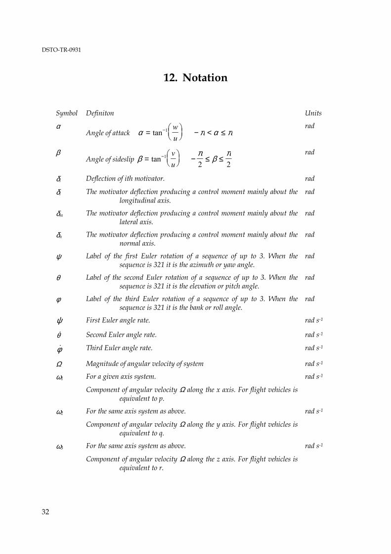
12. Notation
Symbol Definiton Units
α Angle of attack α =
−tan 1 wu
− < ≤π α π rad
β Angle of sideslip β =
−tan 1 vu
− ≤ ≤π
βπ
2 2
rad
δi Deflection of ith motivator. rad
δl The motivator deflection producing a control moment mainly about the longitudinal axis.
rad
δm The motivator deflection producing a control moment mainly about the lateral axis.
rad
δn The motivator deflection producing a control moment mainly about the normal axis.
rad
ψ Label of the first Euler rotation of a sequence of up to 3. When the sequence is 321 it is the azimuth or yaw angle.
rad
θ Label of the second Euler rotation of a sequence of up to 3. When the sequence is 321 it is the elevation or pitch angle.
rad
φ Label of the third Euler rotation of a sequence of up to 3. When the sequence is 321 it is the bank or roll angle.
rad
&ψ First Euler angle rate. rad s-1
&θ Second Euler angle rate. rad s-1
&φ Third Euler angle rate. rad s-1
Ω Magnitude of angular velocity of system rad s-1
ω1 For a given axis system.
Component of angular velocity Ω along the x axis. For flight vehicles is equivalent to p.
rad s-1
ω2 For the same axis system as above.
Component of angular velocity Ω along the y axis. For flight vehicles is equivalent to q.
rad s-1
ω3 For the same axis system as above.
Component of angular velocity Ω along the z axis. For flight vehicles is equivalent to r.
rad s-1
DSTO-TR-0931
33
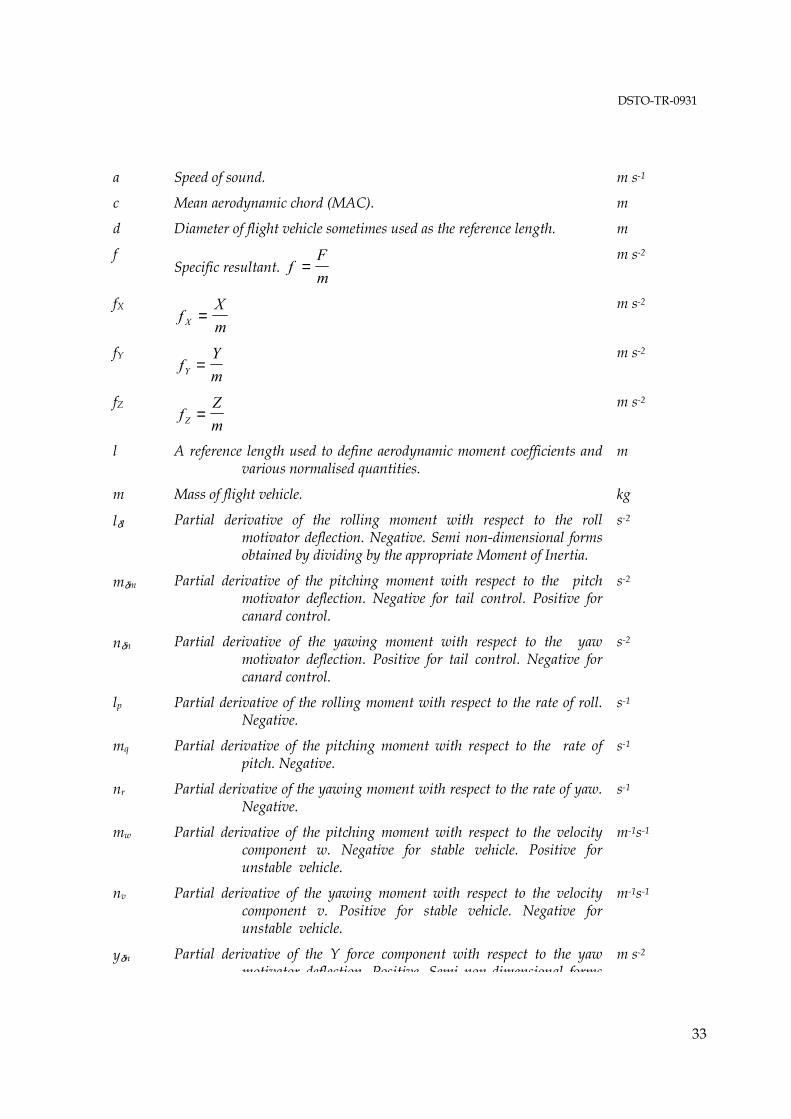
a Speed of sound. m s-1
c Mean aerodynamic chord (MAC). m
d Diameter of flight vehicle sometimes used as the reference length. m
f Specific resultant. f
Fm
= m s-2
fX f
XmX =
m s-2
fY f
YmY =
m s-2
fZ f
ZmZ =
m s-2
l A reference length used to define aerodynamic moment coefficients and various normalised quantities.
m
m Mass of flight vehicle. kg
lδl Partial derivative of the rolling moment with respect to the roll motivator deflection. Negative. Semi non-dimensional forms obtained by dividing by the appropriate Moment of Inertia.
s-2
mδm Partial derivative of the pitching moment with respect to the pitch motivator deflection. Negative for tail control. Positive for canard control.
s-2
nδn Partial derivative of the yawing moment with respect to the yaw motivator deflection. Positive for tail control. Negative for canard control.
s-2
lp Partial derivative of the rolling moment with respect to the rate of roll. Negative.
s-1
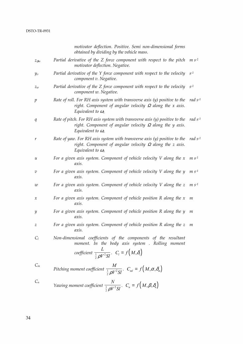
mq Partial derivative of the pitching moment with respect to the rate of pitch. Negative.
s-1
nr Partial derivative of the yawing moment with respect to the rate of yaw. Negative.
s-1
mw Partial derivative of the pitching moment with respect to the velocity component w. Negative for stable vehicle. Positive for unstable vehicle.
m-1s-1
nv Partial derivative of the yawing moment with respect to the velocity component v. Positive for stable vehicle. Negative for unstable vehicle.
m-1s-1
yδn Partial derivative of the Y force component with respect to the yaw motivator deflection Positive Semi non dimensional forms
m s-2
DSTO-TR-0931
34
motivator deflection. Positive. Semi non-dimensional forms obtained by dividing by the vehicle mass.
zδm Partial derivative of the Z force component with respect to the pitch motivator deflection. Negative.
m s-2
yv Partial derivative of the Y force component with respect to the velocity component v. Negative.
s-1
zw Partial derivative of the Z force component with respect to the velocity component w. Negative.
s-1
p Rate of roll. For RH axis system with transverse axis (y) positive to the right. Component of angular velocity Ω along the x axis. Equivalent to ω1.
rad s-1
q Rate of pitch. For RH axis system with transverse axis (y) positive to the right. Component of angular velocity Ω along the y axis. Equivalent to ω2.
rad s-1
r Rate of yaw. For RH axis system with transverse axis (y) positive to the right. Component of angular velocity Ω along the z axis. Equivalent to ω3.
rad s-1
u For a given axis system. Component of vehicle velocity V along the x axis.
m s-1
v For a given axis system. Component of vehicle velocity V along the y axis.
m s-1
w For a given axis system. Component of vehicle velocity V along the z axis.
m s-1
x For a given axis system. Component of vehicle position R along the x axis.
m
y For a given axis system. Component of vehicle position R along the y axis.
m
z For a given axis system. Component of vehicle position R along the z axis.
m
Cl Non-dimensional coefficients of the components of the resultant moment. In the body axis system . Rolling moment
coefficient LV Sl1
22ρ
. ( )C f Ml l= ,δ
Cm Pitching moment coefficient
MV Sl1
22ρ
. ( )C f Mml m= , ,α δ
Cn Yawing moment coefficient
NV Sl1
22ρ
. ( )C f Mn n= , ,β δ

DSTO-TR-0931
35
Cmα Partial derivative of the pitching moment coefficient with respect to the angle of attack. Negative for stable vehicle. Positive for unstable vehicle.
rad-1
Cnβ Partial derivative of the yawing moment coefficient with respect to the sideslip angle. Positive for stable vehicle. Negative for unstable vehicle.
rad-1
Clδl Partial derivative of the rolling moment coefficient with respect to the roll motivator deflection. Negative.
rad-1
Cmδm Partial derivative of the pitching moment coefficient with respect to the pitch motivator deflection. Negative for tail control. Positive for canard control.
rad-1
Cnδn Partial derivative of the yawing moment coefficient with respect to the yaw motivator deflection. Negative for tail control. Positive for canard control.
rad-1
Clp Partial derivative (damping) of the rolling moment coefficient with
respect to the normalised rate of roll. Vis pplV
∗ = .
Negative.
rad-1
Cmq Partial derivative (damping) of the pitching moment coefficient with
respect to the normalised rate of pitch. Vis qqlV
∗ = .
Negative.
rad-1
Cnr Partial derivative (damping) of the yawing moment coefficient with
respect to the normalised rate of yaw. Vis rrlV
∗ = . Negative.
rad-1
Cm &α Partial derivative (damping) of the pitching moment coefficient with respect to the normalised rate of change of the angle of attack.
Vis &&
αα∗ =lV
. Negative.
rad-1
Cn &β Partial derivative (damping) of the yawing moment coefficient with respect to the normalised rate of change of the sideslip angle.
Vis &&
ββ∗ =lV
. Negative.
rad-1
CX X force coefficient
XV S1
22ρ
CY Y force coefficient
YV S1
22ρ
DSTO-TR-0931
36
CZ Z force coefficient
ZV S1
22ρ
CXα Partial derivatives of the force coefficients with respect to the angle of attack.
rad-1
CZα Negative. rad-1
CXβ Partial derivatives of the force coefficients with respect to the sideslip angle
rad-1
CYβ Negative. rad-1
CXδl Partial derivative of the force coefficient with respect to the roll motivator deflection.
rad-1
CYδn Partial derivative of the force coefficient with respect to the yaw motivator deflection. Positive.
rad-1
CZδm Partial derivative of the force coefficient with respect to the pitch motivator deflection. Negative.
rad-1
F The resultant of the airframe aerodynamic forces acting on the vehicle. N
Ix
(A)
Moments of Inertia with respect to the body axes. Moment of inertia about the x axis. (longitudinal).
kg m2
Iy
(B)
Moment of inertia about the y axis. (lateral). kg m2
Iz
(C)
Moment of inertia about the z axis. (normal). kg m2
Izx or Ixz
(D)
Products of Inertia with respect to the body axes. kgm2
Iyz or Izy
(E)
kg m2
Ixy or Iyx
(F)
kg m2
M Mach number M V a= /
L Components of the resultant moment Q. In the body axis system. Rolling moment.
N m
M Pitching moment. N m
N Yawing moment. N m
Lδl Partial derivative of the rolling moment with respect to the roll motivator deflection. Negative.
N m rad-1-
DSTO-TR-0931
37
Mδm Partial derivative of the pitching moment with respect to the pitch motivator deflection. Negative for tail control. Positive for canard control.
N m rad-1
Nδn Partial derivative of the yawing moment with respect to the yaw motivator deflection. Positive for tail control. Negative for canard control.
N m rad-1
Lp Partial derivative of the rolling moment with respect to the rate of roll. Negative.
N m s rad-1
Mq Partial derivative of the pitching moment with respect to the rate of pitch. Negative.
N m s rad-1
Nr Partial derivative of the yawing moment with respect to the rate of yaw. Negative.
N m s rad-1
Mw Partial derivative of the pitching moment with respect to the. velocity component w. Negative for stable vehicle. Positive for unstable vehicle.
N s
Nv Partial derivative of the yawing moment with respect to the velocity component v. Positive for stable vehicle. Negative for unstable vehicle.
N s
Q The resultant moment of the resultant force F about a reference point. Usually the centre of mass.
N m
S Reference Area. m2
X Components of the resultant force F. In the body axis system. Component along the x axis. (longitudinal).
N
Y Component along the y axis. (lateral). N
Z Component along the z axis. (normal). N
Yδn Partial derivative of the Y force component with respect to the yaw motivator deflection. Positive.
N rad-1
Zδm Partial derivative of the Z force component with respect to the pitch motivator deflection. Negative.
N rad-1
Yv Partial derivative of the Y force component with respect to the velocity component v. Negative.
N s m-1
Zw Partial derivative of the Z force component with respect to the velocity component w. Negative.
N s m-1

DSTO-TR-0931
38
Entity or reference Axis system Symbol
Geocentric Earth-fixed The origin is fixed at the centre of the Earth, the x axis passes through the intersection of the Greenwich meridian and the equator and the z axis is the mean spin axis of the Earth, positive to the North the y axis completes the right-handed system.
G
Normal Earth-fixed A right-hand coordinate system, fixed relative to and rotating with the Earth, with the origin chosen as appropriate, the z axis is parallel to the downward vertical, positive down and the x axis is chosen as appropriate.
E
Vehicle carried normal Earth A system in which each axis is parallel to the corresponding normal Earth-fixed axis, with the origin usually fixed at the centre of mass of the vehicle.
E
Sensor (IR, RF, Optical etc) The origin is fixed at the sensing element which is usually assumed to be at the centre of mass of the vehicle. The x axis passes through the centre of the field-of-view, the y axis in or parallel to some reference plane and the z axis completes a right-handed set.
D
Seeker/tracker reference A right-hand coordinate system, fixed but not necessarily aligned relative to the vehicle/platform body, with the origin at the sensing element.
S
Line-of-sight The origin is fixed in the centre of mass of the reference platform. The x axis is coincident with the range vector and positive out, the y axis is horizontal and positive to the right and the z axis completes a right-handed set.
L
Flight vehicle body The origin is fixed at the centre of mass of the vehicle. The x or longitudinal axis is in or parallel to the reference plane, and positive forward. The y or lateral axis is normal to the reference plane and positive to the right. The z or normal axis is in or parallel to the reference plane and completes a right-handed set. eg Missile
M
DSTO-TR-0931
39
(M).
Autopilot This is normally the same as the body system but may be rotated about the x axis relative to the body system.
P
Air path a
Intermediate e
Total angle of attack t
Flight path The origin is fixed at the centre of mass and the x axis is in the direction of the flight path velocity. The y and z axes are chosen to be consistent with the right-handed convention.
F
Attacker The attackerr model is usually 3 DOF so a flight path axis system is used.
A
Target The target model is usually 3 DOF so a flight path axis system is used.
T
Illuminator It may be on the launcher or on a separate platform. I
HIL System reference The origin is fixed at the centre of rotation of the motion table. The axes form a right-handed set. The direction of the x axes depends on the table location, however it passes through the centre of the scene generator.
R
HIL Table payload This frame is coincident with the HIL frame rotated 180 degrees anticlockwise about the HIL x axis.
P
HIL scene generator This is coincident with the HIL reference frame. C
HIL variable window This frame links the hardware and software spaces. It is coincident with the HIL reference frame in hardware space and can be tied to any frame in software space.
V

DSTO-TR-0931
40
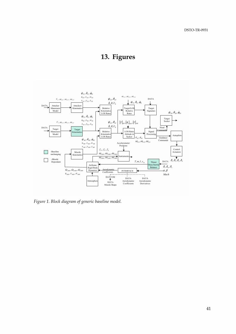
DSTO-TR-0931
41
13. Figures
TargetManoeurer
Model
& , , ,VT TT TT TTω ω ω1 2 3
& , & , &
, ,, ,
ψ θ φTE TE TE
TE TE TE
TE TE TE
u v wx y z
AttackerManoeurer
Model
AttackerrKinematics
& , , ,VF FF FF FFω ω ω1 2 3
& , & , &
, ,, ,
ψ θ φFE FE FE
FE FE FE
FE FE FE
u v wx y z
MissileKinematics
& , & , && , & , &ω ω ω1 2 3MM MM MM
MM MM MMu v w
& , & , &
, ,, ,
ψ θ φME ME ME
ME ME ME
ME ME ME
u v wx y z
DATA
DATA
RelativeKinematicsLOS Rates
R
LELE
VRR ,,
,&
&& θψ
RelativeKinematicsLOS Rates
R
LELE
VRR ,,
,&
&& θψ
Target/LOSRelative
Rates
ω ω ω1 2 3TT TT TT, ,
& , & , &ψ θ φTL TL TL
LOS RatesAttitude in
Seeker ε εω ω ωAZ EL
LS LS LS
,, ,1 2 3
SignalProcessing
TargetSignature
TargetSeeker
SDSDSD φθψ &&& ,,
[ ] [ ] [ ] MESMSD TRT ,, 1
Autopilots
ControlActuators
AirframeRigid BodyDynamics
DATAAerodynamicCoefficients
DATAAerodynamicDerivatives
DATCOM
DATAMissile Shape
INTERFACE
Atmosphere
AerodynamicCoefficients
ThrustMass/Inertia
Balance
DATA
DATA
InstrumentsMMMMMM
MMMMMM
ZYX fff
321
321
,,,,
,,
ωωωωωω &&&
Mach
nml
βαδδδ
,,,
T m I xcg, , ,
AccelerometerPositions
TargetKinematics
GuidanceCommands
HeadCommands
-Baselineunchanging
-Missile Dependant 4231 ,,, δδδδ
Figure 1. Block diagram of generic baseline model.

DSTO-TR-0931
42
YS
ZS
XS,XM
YM
ZM
Motivator 3(UP)
Motivator 1
Motivator 2(RIGHT)
Motivator 4
UmbilicalLOOKINGFORWARD
Gimbals
Figure 2. Seeker reference and missile body coordinate systems.
YM , jM
XE
YE
ZE , kE
XM , iM
YM , jM ZM , kM
pM
qM
rM
ψΜΕ
φME
θΜΕ
ZM
!
!
"
!
"
"
MEθ&
MEψ&
MEφ&
Figure 3. Missile body axes rotation rate components.
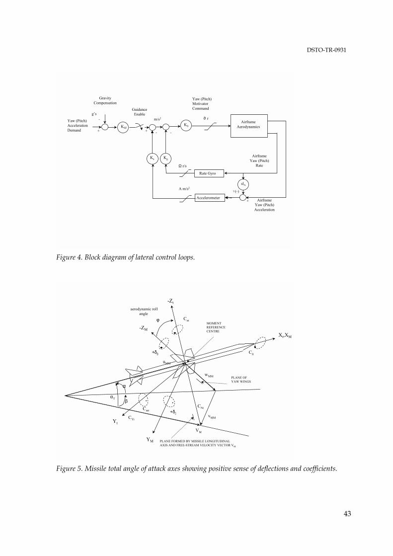
DSTO-TR-0931
43
+
-
+
KSF
Ka
GravityCompensation
ϑ r
Accelerometer
+
gsm/s2
Yaw (Pitch)MotivatorCommand
AirframeYaw (Pitch)
Rate
AirframeYaw (Pitch)Acceleration
Yaw (Pitch)AccelerationDemand
Kg
A m/s2
KS
Rate Gyro
Ω r/s
AirframeAerodynamics
slA
+(-)
GuidanceEnable
--
Figure 4. Block diagram of lateral control loops.
-Zt
-ZM
Yt
YM
Xt,XM
vMM
wMM
uMM
VM
CNt
CYt
+δ3
+δ2Cmt
Cnt
Clt
MOMENTREFERENCE CENTRE
PLANE OF YAW WINGS
αT
PLANE FORMED BY MISSILE LONGITUDINAL AXIS AND FREE-STREAM VELOCITY VECTOR VM
""
!
!
!
β
α
φ
aerodynamic rollangle
Figure 5. Missile total angle of attack axes showing positive sense of deflections and coefficients.

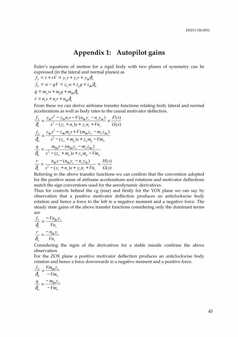
DSTO-TR-0931
45
Appendix 1: Autopilot gains
Eulers equations of motion for a rigid body with two planes of symmetry can be expressed (in the lateral and normal planes) as f v rV y v y r yY v r n n= + = + +& δ δ f w qV z w z q zZ w q m m= − = + +& δ δ &q m w m q mw q m m= + + δ δ &r n v n r nv r n n= + + δ δ
From these we can derive airframe transfer functions relating body lateral and normal accelerations as well as body rates to the causal motivator deflection. f y s y n s V n y n y
s y n s y n VnF sG s
Y
n
n n r n v v n
v r v r vδδ δ δ δ=
− − −− + + +
=2
2
( )( )
( )( )
f z s z m s V m z m zs z m s z m Vm
Z
m
m m q m w w m
w q w q wδδ δ δ δ=
− + −− + + −
2
2
( )( )
q m s m z m zs z m s z m Vmm
m m w w m
w q w q wδδ δ δ= − −
− + + −( )
( )2
r n s n y n ys y n s y n Vn
H sG sn
n n v v n
v r v r vδδ δ δ=
− −− + + +
=( )
( )( )( )2
Referring to the above transfer functions we can confirm that the convention adopted for the positive sense of airframe accelerations and rotations and motivator deflections match the sign conventions used for the aerodynamic derivatives. Thus for controls behind the cg (rear) and firstly for the YOX plane we can say by observation that a positive motivator deflection produces an anticlockwise body rotation and hence a force to the left ie a negative moment and a negative force. The steady state gains of the above transfer functions considering only the dominant terms are f Vn y
VnY
n
n v
vδδ=
−
v
vn
n Vnynr δ
δ−=
Considering the signs of the derivatives for a stable missile confirms the above observation. For the ZOX plane a positive motivator deflection produces an anticlockwise body rotation and hence a force downwards ie a negative moment and a positive force. f Vm z
VmZ
m
m w
wδδ=
−
q m zVmm
m w
wδδ=
−−

DSTO-TR-0931
46
As above these expressions for the steady state gains confirm the observation. For forward controls we have by observation that in the YOX plane a positive motivator deflection produces a clockwise moment and hence a force to the right while in the ZOX plane a positive motivator deflection produces a clockwise moment and hence a force upwards. These observations are confirmed by the above steady state gains. The autopilot configuration that will be used initially is a basic form of the widely used proportional configuration for control in the missile body lateral and normal planes. The high frequency dynamics of the control actuator servos and measuring instruments as well as lag-lead network are not considered here so the model is a low frequency model as shown in figure 4. It is useful to establish the signs of the gains in the autopilot. Assuming positive acceleration demands and positive values for the scale factor gain. Consider the gains for rear control and in the YOX plane. A positive body acceleration requires a negative motivator deflection hence Ks must be negative. The feedback signal at the summing point must be positive so Ka is positive. A negative motivator deflection will produce a positive body rotation so Kg must be positive. The signs can be similarly established for the other plane and for forward controls as in the table below.
Plane KSF Ks Ka Kg Rear YOX + - + +
Controls ZOX + + + - Forward YOX + + + + Controls ZOX + - + -
If the accelerometer is not located at the cg then it will sense both the normal acceleration of the missile cg as well as a tangential acceleration due to body angular accelerations. The acceleration that is sensed in the YOX plane is f l rY A+ & , where lA is the position of the accelerometer relative to the cg (+ve forward). And in the ZOX plane it is f l qZ A− & . In fact locating the accelerometer away from the cg has a stabilising influence providing it is in the right direction. Also there is a critical position that simplifies the compensation for high frequency effects of fin servo, sensor and body bending. Thus the sensor should be located further from the cg than this critical distance given by
lyn
Im x xa
n
n
Z
m CG=
−=
−δ
δ ( )
where IZ is the moment of inertia about the Z (yaw) axis m is the missile mass xm is the control surface centre of pressure position aft of the nose xCG is the centre of gravity position aft of the nose
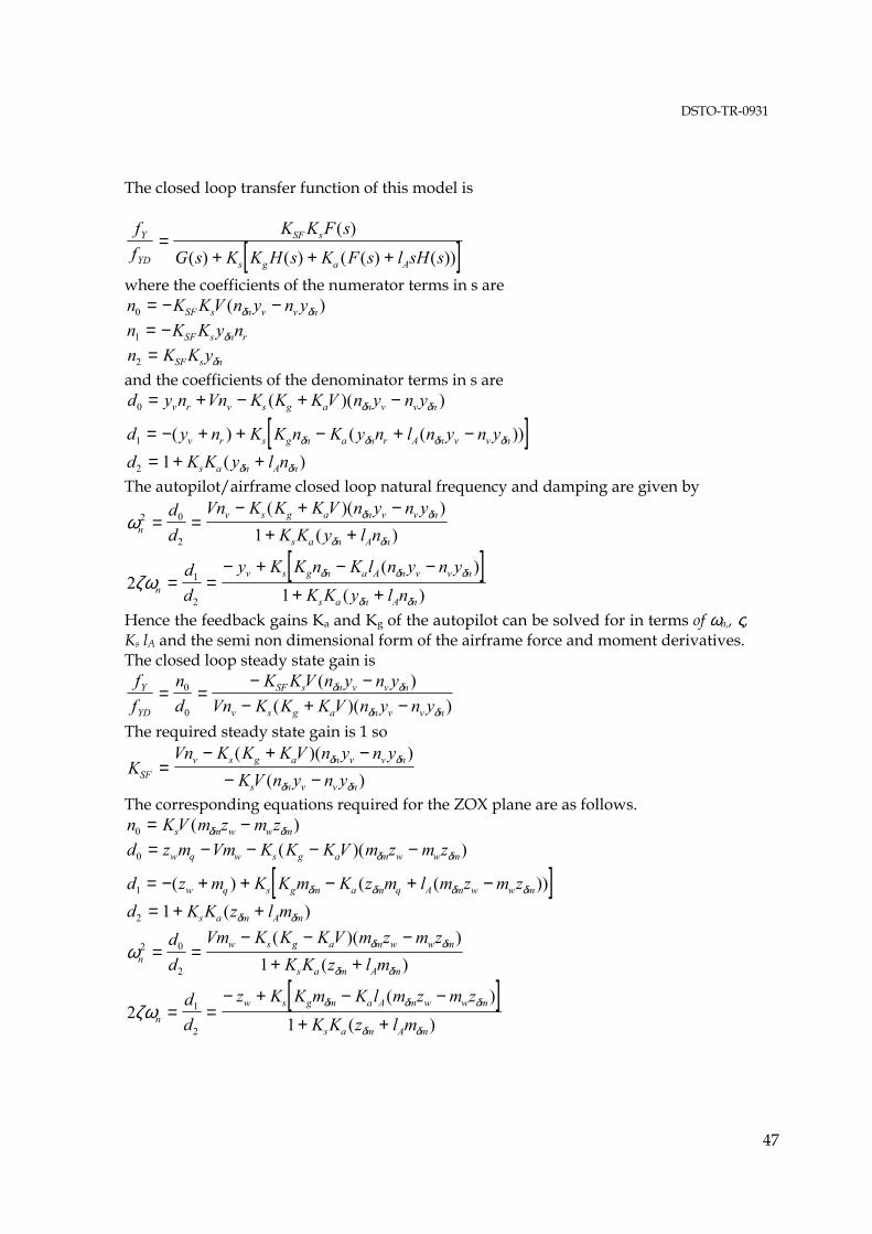
DSTO-TR-0931
47
The closed loop transfer function of this model is
[ ]ff
K K F s
G s K K H s K F s l sH sY
YD
SF s
s g a A
=+ + +
( )
( ) ( ) ( ( ) ( ))
where the coefficients of the numerator terms in s are n K KV n y n ySF s n v v n0 = − −( )δ δ n K K y nSF s n r1 = − δ n K K ySF s n2 = δ and the coefficients of the denominator terms in s are d y n Vn K K K V n y n yv r v s g a n v v n0 = + − + −( )( )δ δ
[ ]d y n K K n K y n l n y n yv r s g n a n r A n v v n1 = − + + − + −( ) ( ( ))δ δ δ δ
d K K y l ns a n A n2 1= + +( )δ δ The autopilot/airframe closed loop natural frequency and damping are given by
ω δ δ
δ δn
v s g a n v v n
s a n A n
dd
Vn K K K V n y n yK K y l n
2 0
2 1= =
− + −+ +( )( )
( )
[ ]2
11
2ζω δ δ δ
δ δn
v s g n a A n v v n
s a n A n
dd
y K K n K l n y n yK K y l n
= =− + − −
+ +( )
( )
Hence the feedback gains Ka and Kg of the autopilot can be solved for in terms of ωn,, ς, Ks lA and the semi non dimensional form of the airframe force and moment derivatives. The closed loop steady state gain is ff
nd
K KV n y n yVn K K K V n y n y
Y
YD
SF s n v v n
v s g a n v v n= =
− −− + −
0
0
( )( )( )
δ δ
δ δ
The required steady state gain is 1 so
KVn K K K V n y n y
KV n y n ySFv s g a n v v n
s n v v n=
− + −− −
( )( )( )
δ δ
δ δ
The corresponding equations required for the ZOX plane are as follows. n KV m z m zs m w w m0 = −( )δ δ d z m Vm K K K V m z m zw q w s g a m w w m0 = − − − −( )( )δ δ
[ ]d z m K K m K z m l m z m zw q s g m a m q A m w w m1 = − + + − + −( ) ( ( ))δ δ δ δ
d K K z l ms a m A m2 1= + +( )δ δ
ω δ δ
δ δn
w s g a m w w m
s a m A m
dd
Vm K K K V m z m zK K z l m
2 0
2 1= =
− − −+ +( )( )
( )
[ ]2
11
2ζω δ δ δ
δ δn
w s g m a A m w w m
s a m A m
dd
z K K m K l m z m zK K z l m
= =− + − −
+ +( )
( )
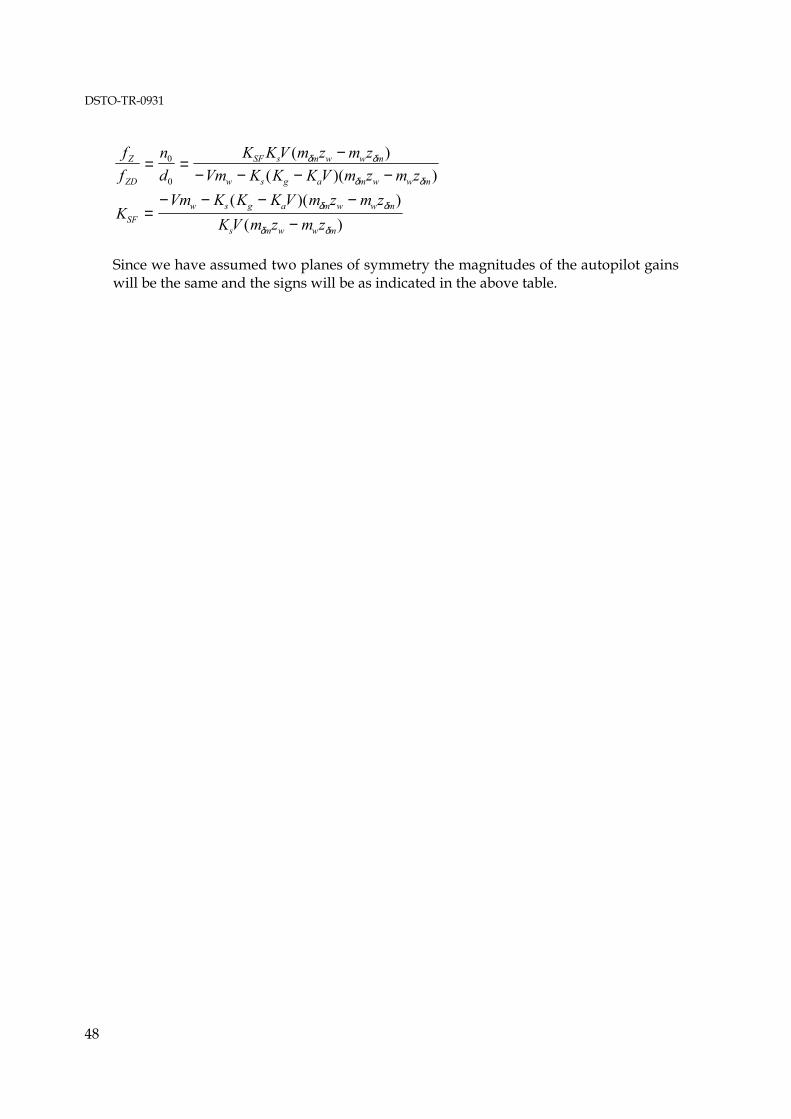
DSTO-TR-0931
48
ff
nd
K KV m z m zVm K K K V m z m z
Z
ZD
SF s m w w m
w s g a m w w m= =
−− − − −
0
0
( )( )( )
δ δ
δ δ
KVm K K K V m z m z
KV m z m zSFw s g a m w w m
s m w w m=
− − − −−
( )( )( )
δ δ
δ δ
Since we have assumed two planes of symmetry the magnitudes of the autopilot gains will be the same and the signs will be as indicated in the above table.
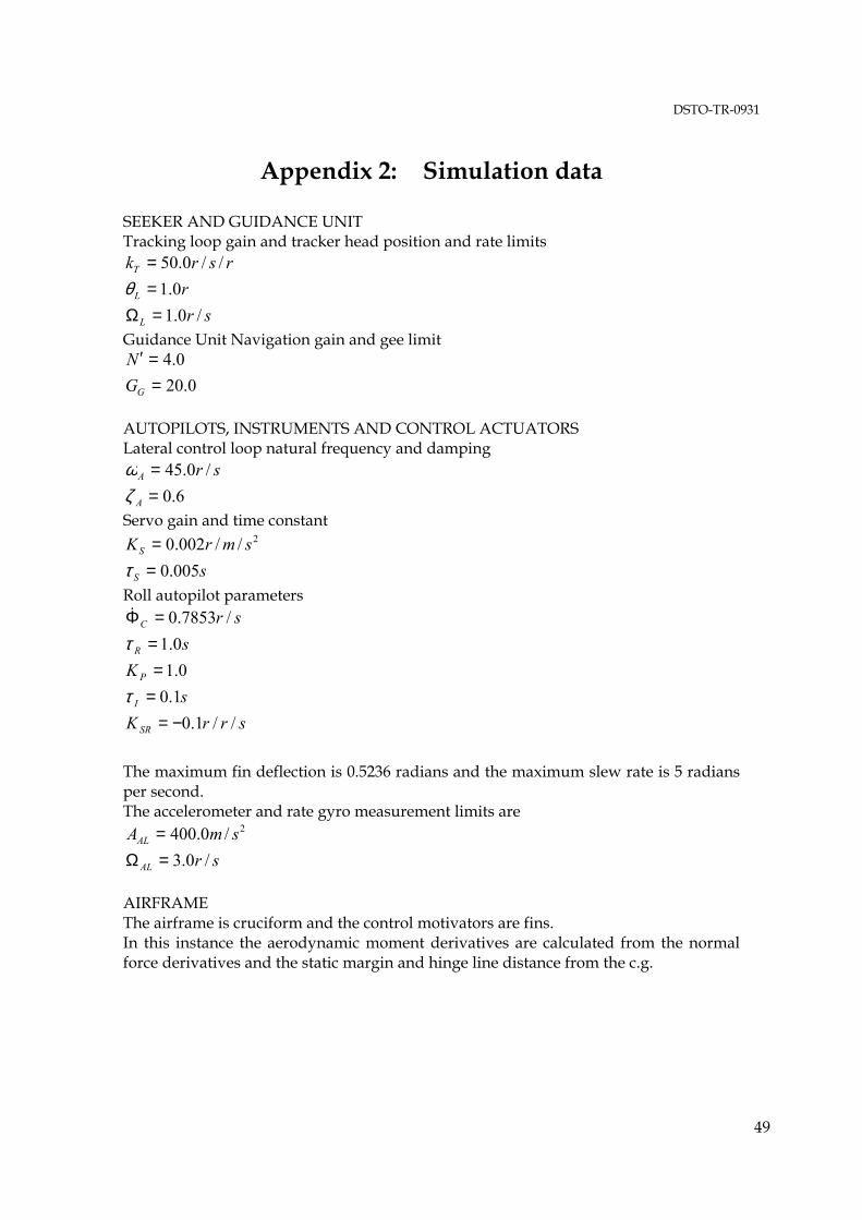
DSTO-TR-0931
49
Appendix 2: Simulation data
SEEKER AND GUIDANCE UNIT Tracking loop gain and tracker head position and rate limits
srr
rsrk
L
L
T
/0.10.1
//0.50
=Ω==
θ
Guidance Unit Navigation gain and gee limit
0.200.4
==′
GGN
AUTOPILOTS, INSTRUMENTS AND CONTROL ACTUATORS Lateral control loop natural frequency and damping
6.0/0.45
==
A
A srζω
Servo gain and time constant
ssmrK
S
S
005.0//002.0 2
==
τ
Roll autopilot parameters
srrKs
Ks
sr
SR
I
P
R
C
//1.01.00.1
0.1/7853.0
−===
==Φ
τ
τ
&
The maximum fin deflection is 0.5236 radians and the maximum slew rate is 5 radians per second. The accelerometer and rate gyro measurement limits are
srsmA
AL
AL
/0.3/0.400 2
=Ω=
AIRFRAME The airframe is cruciform and the control motivators are fins. In this instance the aerodynamic moment derivatives are calculated from the normal force derivatives and the static margin and hinge line distance from the c.g.
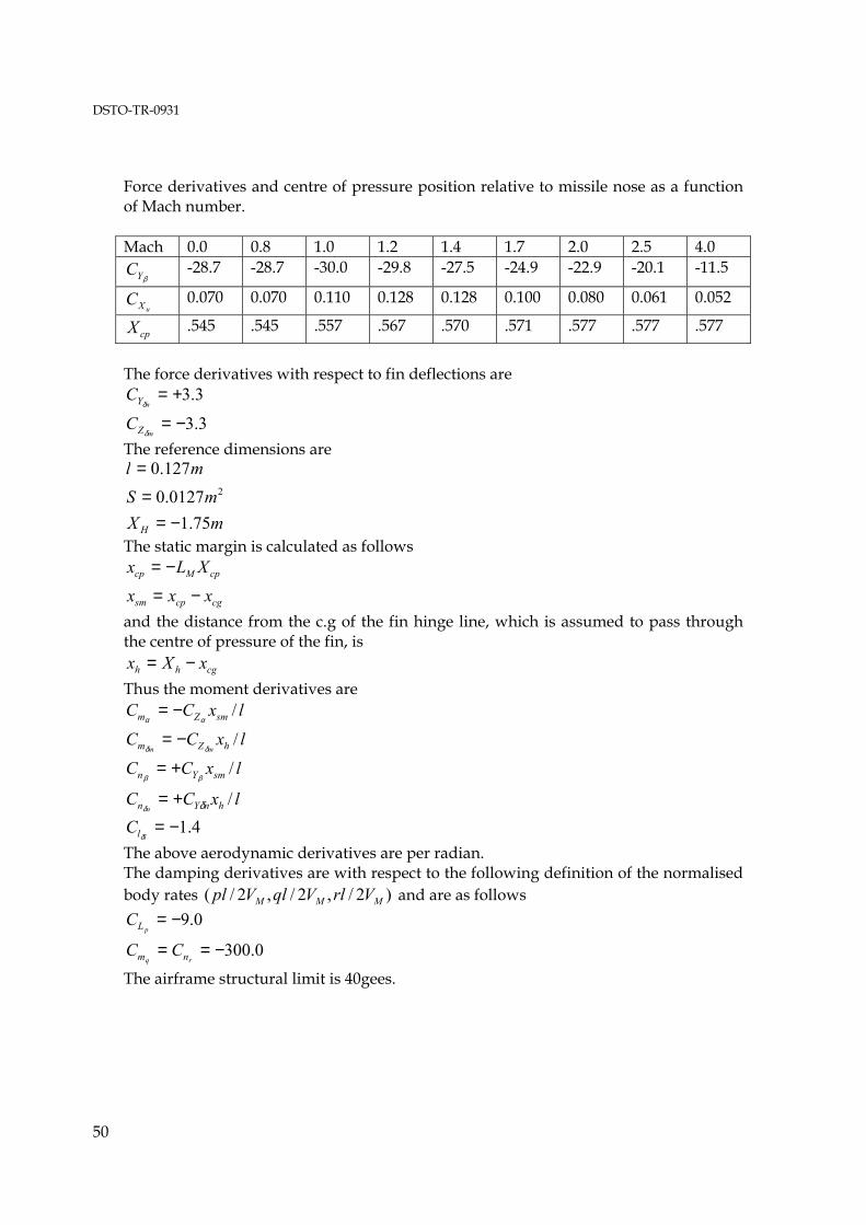
DSTO-TR-0931
50
Force derivatives and centre of pressure position relative to missile nose as a function of Mach number. Mach 0.0 0.8 1.0 1.2 1.4 1.7 2.0 2.5 4.0
βYC -28.7 -28.7 -30.0 -29.8 -27.5 -24.9 -22.9 -20.1 -11.5
uXC 0.070 0.070 0.110 0.128 0.128 0.100 0.080 0.061 0.052
cpX .545 .545 .557 .567 .570 .571 .577 .577 .577
The force derivatives with respect to fin deflections are
3.3
3.3
−=
+=
m
n
Z
Y
C
C
δ
δ
The reference dimensions are
mXmS
ml
H 75.10127.0
127.02
−==
=
The static margin is calculated as follows
cgcpsm
cpMcp
xxx
XLx
−=
−=
and the distance from the c.g of the fin hinge line, which is assumed to pass through the centre of pressure of the fin, is
cghh xXx −= Thus the moment derivatives are
lxCC
lxCC
lxCC
lxCC
hnYn
smYn
hZm
smZm
n
mm
/
/
/
/
δδ
ββ
δδ
αα
+=
+=
−=
−=
4.1−=ll
Cδ
The above aerodynamic derivatives are per radian. The damping derivatives are with respect to the following definition of the normalised body rates )2/,2/,2/( MMM VrlVqlVpl and are as follows
0.300
0.9
−==
−=
rq
p
nm
L
CC
C
The airframe structural limit is 40gees.
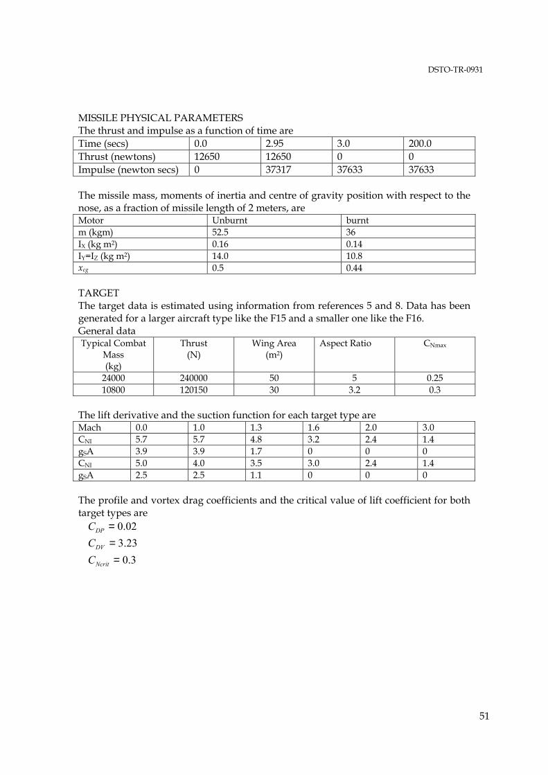
DSTO-TR-0931
51
MISSILE PHYSICAL PARAMETERS The thrust and impulse as a function of time are Time (secs) 0.0 2.95 3.0 200.0 Thrust (newtons) 12650 12650 0 0 Impulse (newton secs) 0 37317 37633 37633 The missile mass, moments of inertia and centre of gravity position with respect to the nose, as a fraction of missile length of 2 meters, are Motor Unburnt burnt m (kgm) 52.5 36 IX (kg m2) 0.16 0.14 IY=IZ (kg m2) 14.0 10.8 xcg 0.5 0.44 TARGET The target data is estimated using information from references 5 and 8. Data has been generated for a larger aircraft type like the F15 and a smaller one like the F16. General data Typical Combat
Mass (kg)
Thrust (N)
Wing Area (m2)
Aspect Ratio CNmax
24000 240000 50 5 0.25 10800 120150 30 3.2 0.3
The lift derivative and the suction function for each target type are Mach 0.0 1.0 1.3 1.6 2.0 3.0 CNI 5.7 5.7 4.8 3.2 2.4 1.4 gSA 3.9 3.9 1.7 0 0 0 CNI 5.0 4.0 3.5 3.0 2.4 1.4 gSA 2.5 2.5 1.1 0 0 0 The profile and vortex drag coefficients and the critical value of lift coefficient for both target types are
3.023.302.0
===
Ncrit
DV
DP
CCC
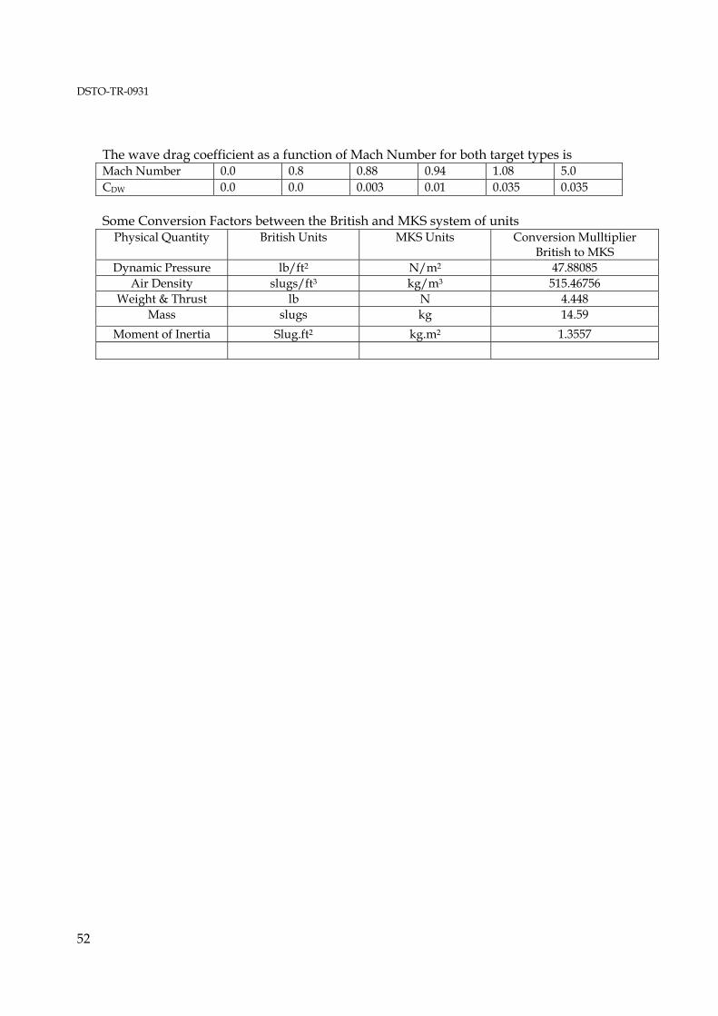
DSTO-TR-0931
52
The wave drag coefficient as a function of Mach Number for both target types is Mach Number 0.0 0.8 0.88 0.94 1.08 5.0 CDW 0.0 0.0 0.003 0.01 0.035 0.035 Some Conversion Factors between the British and MKS system of units
Physical Quantity British Units MKS Units Conversion Mulltiplier British to MKS
Dynamic Pressure lb/ft2 N/m2 47.88085 Air Density slugs/ft3 kg/m3 515.46756
Weight & Thrust lb N 4.448 Mass slugs kg 14.59
Moment of Inertia Slug.ft2 kg.m2 1.3557
Page classification: UNCLASSIFIED
DEFENCE SCIENCE AND TECHNOLOGY ORGANISATION
DOCUMENT CONTROL DATA 1. PRIVACY MARKING/CAVEAT (OF DOCUMENT)
2. TITLE A Baseline 6 Degree of Freedom (DOF) Mathematical Model of a Generic Missile
3. SECURITY CLASSIFICATION (FOR UNCLASSIFIED REPORTS THAT ARE LIMITED RELEASE USE (L) NEXT TO DOCUMENT CLASSIFICATION) Document (U) Title (U) Abstract (U)
4. AUTHOR(S) R. M. Gorecki
5. CORPORATE AUTHOR Systems Sciences Laboratory PO Box 1500 Edinburgh South Australia 5111 Australia
6a. DSTO NUMBER DSTO-TR-0931
6b. AR NUMBER AR-012-934
6c. TYPE OF REPORT Technical Report
7. DOCUMENT DATE July 2003
8. FILE NUMBER J 9505/17/214
9. TASK NUMBER LRR 02/186
10. TASK SPONSOR CWSD
11. NO. OF PAGES 50
12. NO. OF REFERENCES 8
13. URL on the World Wide Web http://www.dsto.defence.gov.au/corporate/reports/DSTO-TR-0931.pdf
14. RELEASE AUTHORITY Chief, Weapons Systems Division
15. SECONDARY RELEASE STATEMENT OF THIS DOCUMENT
Approved for public release OVERSEAS ENQUIRIES OUTSIDE STATED LIMITATIONS SHOULD BE REFERRED THROUGH DOCUMENT EXCHANGE, PO BOX 1500, EDINBURGH, SA 5111 16. DELIBERATE ANNOUNCEMENT
No Limitation. 17. CITATION IN OTHER DOCUMENTS Yes 18. DEFTEST DESCRIPTORS
Mathematical models, Missile Simulation, Hardware in the loop 19. ABSTRACT This report describes a 6 degree-of-freedom mathematical model of a generic missile engagement. The model is to be used as a baseline or template for missile 6 DOF computer simulation models. This documentation will form part of the documentation for all derived models
Page classification: UNCLASSIFIED