816 IEEE TRANSACTIONS ON GEOSCIENCE AND …ktb.engin.umich.edu/...Kroodsma-etal_Vicarious-Cal-Conical-Imagers.pdf · Vicarious Cold Calibration for Conical ... VCC has been shown

816 IEEE TRANSACTIONS ON GEOSCIENCE AND REMOTE SENSING, VOL. 55, NO. 2, FEBRUARY 2017

Vicarious Cold Calibration for ConicalScanning Microwave Imagers

Rachael A. Kroodsma, Member, IEEE, Darren S. McKague, and Christopher S. Ruf, Fellow, IEEE

Abstract— Vicarious cold calibration (VCC) for spacebornemicrowave radiometers is analyzed and modified for applicationto conical scanning microwave imagers at frequencies from6 to 90 GHz. The details of the algorithm are modified toaccount for additional frequencies and polarizations that werenot included in the development of the original algorithm.The modified algorithm is shown to produce a more stablecold reference brightness temperature (TB) than the originalalgorithm. An analysis is performed of this updated algorithmto show the global regions that contribute to the derivation ofthe cold reference TB and to show which geophysical parameterscontribute to the coldest TBs. The analysis suggests that watervapor variability has the largest impact on the TBs in the VCCalgorithm. The modified VCC algorithm is applied to microwaveimager data and is used as an intercalibration method. It is shownto agree well with other intercalibration methods, demonstratingthat it is a valid and accurate method for calibration of microwaveimagers.

Index Terms— AMSR2, calibration, intercalibration,Microwave radiometry, TMI.

I. INTRODUCTION

M ICROWAVE radiometers onboard satellites providevaluable observations of the earth’s surface and

atmosphere. These observations are in the form of brightnesstemperature (TB) measurements that are input to models toretrieve numerous geophysical parameters, such as surfacetemperature, surface wind speed (SWS), and atmosphericwater vapor. In order to retrieve accurate geophysical parame-ters, the radiometer TB measurements must first be properlycalibrated before they are used as inputs to geophysicalretrieval algorithms. Microwave radiometers typically havean on-board calibration system to calibrate the instrumentwhile it is in flight to convert from raw counts into antennatemperatures. The antenna temperatures are then convertedinto TBs through an antenna pattern correction. In addition tothe on-board calibration of the radiometer, the TBs measuredfrom the earth can also be used to monitor the calibration of theradiometer. Using these TBs provides a calibration reference

Manuscript received January 20, 2016; revised June 24, 2016; acceptedAugust 24, 2016. Date of publication October 24, 2016; date of current versionDecember 29, 2016.

R. A. Kroodsma is with the Earth System Science Interdisciplinary Center,University of Maryland, College Park, MD 20740 USA, and also with theNASA Goddard Space Flight Center, Greenbelt, MD 20771 USA (e-mail:[email protected]).

D. S. McKague and C. S. Ruf are with the University of Michigan, AnnArbor, MI 48109 USA (e-mail: [email protected]; [email protected]).

Color versions of one or more of the figures in this paper are availableonline at http://ieeexplore.ieee.org.

Digital Object Identifier 10.1109/TGRS.2016.2615552

for the instrument that is performed through the radiometer’sreflector and can be used to detect calibration issues such aserrors in the antenna pattern correction, obstructions in thefield of view, or drifts in the on-board calibration system.

Vicarious cold calibration (VCC) is one method that usesan external earth target to calibrate a spaceborne microwaveradiometer [1]. VCC uses histograms of the TB observationsto derive a stable cold reference point, referred to as the“cold cal TB.” VCC has been shown to be a valuable tool formicrowave radiometer calibration by detecting drifts in theradiometer measurements [2], correcting obstructions in thefield of view [3], and deriving intercalibration offsets [4], [5].Previous studies [3]–[5] applied VCC to conical scanningmicrowave imagers, even though the original algorithmdescribed in [1] was for use with a nadir-viewing microwaveradiometer over a more narrow range of frequencies. Thesestudies used a modified VCC algorithm different from theoriginal and obtained quality results, but the changes madeto the algorithm were not described nor was the modifiedalgorithm analyzed to confirm that it was better able to achievea stable cold cal TB in the conical scanning case.

This paper discusses the application of VCC to conicalscanning microwave imagers and provides an in-depth analy-sis of various aspects of the VCC algorithm, including adescription of how the VCC algorithm is modified. First,the VCC algorithm details are examined and modificationsare made to the original algorithm to make it applicableto conical scanners. Second, the geophysical parameters thatcontribute to the derivation of the cold cal TB are examined.Third, the VCC algorithm is applied to microwave imagerdata to show its use as a relative calibration tool. Finally, themodified VCC algorithm is validated by using it to intercali-brate microwave radiometers and demonstrate that it achievescomparable results with other intercalibration methods.

II. VCC ALGORITHM

The original VCC algorithm was designed to be usedwith a nadir-viewing microwave radiometer at 18, 21, and37 GHz [1]. The algorithm derives a stable cold referenceusing TB histograms of over-ocean observations. To derivethis cold reference, a “first-guess” value is found for eachfrequency. This is the theoretical coldest TB derived froma radiative transfer model (RTM). The radiometer observedTBs that fall within ±10 K of this first-guess are binned intohistograms for each channel at 0.1 K intervals. A third-degreepolynomial is then fit to 3%–10% of the cumulative distribu-tion function (CDF) of this histogram and the polynomial is

0196-2892 © 2016 IEEE. Personal use is permitted, but republication/redistribution requires IEEE permission.See http://www.ieee.org/publications_standards/publications/rights/index.html for more information.

KROODSMA et al.: VCC FOR CONICAL SCANNING MICROWAVE IMAGERS 817

Fig. 1. AMSR2 TB histograms for one month of over-ocean observations.

extrapolated down to 0%, where the TB value at 0% CDF isthe cold cal TB. These details of the original VCC algorithmwere chosen to achieve the most stable cold reference for aspecific nadir-viewing radiometer. However, these details maynot result in the most stable cold cal TB for conical scanningimagers. This section discusses modifications that are made tothe original VCC algorithm to make it applicable to conicalscanning imagers and shows the improvement of the modifiedalgorithm over the original one.

A. Conical Scanning Microwave Imager Observations

One major difference between conical scanning and nadir-viewing radiometers is the angle at which they view theearth. Conical scanners have a reflector that is offset fromnadir, resulting in a nonzero earth incidence angle (EIA)and a signal received from earth’s surface that is polarized.A second major difference is the polarization of the TBmeasurements. Conical scanners observe distinct vertical (V)and/or horizontal (H) polarized TBs at each frequency whilenadir-viewing radiometers do not observe a polarized signal.The frequencies of conical scanners vary for each instrumentbased on specific design requirements but most have frequen-cies near 18, 21, and 37 GHz. Other frequencies typicallyincluded are near 7, 11, and 90 GHz, so all of these frequenciesshould be considered when developing a new VCC algorithm.Conical scanners can include frequencies higher than 90 GHz;however, these frequencies see less of the surface due to ahigher sensitivity to the atmospheric water vapor. This makesit very difficult for VCC to derive a stable cold reference,so these higher frequencies are not discussed here.

The VCC algorithm calculates the cold cal TB from his-tograms of over-ocean TBs. The shape of the histograms caninfluence the stability of the cold cal TB, so it is valuable toexamine how the histograms differ as a function of frequencyand polarization. This is shown here using TB observa-tions from the Advanced Microwave Scanning Radiome-ter 2 (AMSR2). AMSR2 is a conically scanning microwaveradiometer that observes at 6.925, 7.3, 10.65, 18.7, 23.8, 36.5,and 89.0 GHz, with vertical and horizontal polarizations at allfrequencies [6]. Fig. 1 shows TB histograms for one month ofover-ocean observations for 12 of the 16 AMSR2 channels.

The 7.3 and 89.0b GHz channels are excluded since theyare nearly identical to the 6.925 and 89.0a GHz channels,respectively.

Fig. 1 illustrates the variation in the TB histograms acrossthe frequency spectrum. Some of the channels, such as6.9 and 10.65 H, show one very steep peak with the majorityof the observations occurring over a small range of TBs, whileother channels, such as 23.8 and 89.0 H, have histogramswith a more uniform distribution across a wide dynamic rangeof TBs. Since the shapes of the histograms vary by channel, thebest VCC algorithm will most likely be different, dependingon the channel to which the algorithm is applied.

B. Development of Modified VCC Algorithm

This section describes the development of the modified VCCalgorithm for application to conical scanners. The applicationof the modified algorithm to AMSR2 is shown as an example.

1) Algorithm Details: The VCC algorithm can be dividedinto four steps: 1) calculate a first-guess for each channel;2) bin the TBs into histograms for a range of ±10 K fromthe first-guess; 3) calculate the CDF for each histogram andtake 3%–10% of the CDF (called the CDF subset); and4) fit a third-order polynomial to the inverse CDF subset andextrapolate down to 0%. Each of these steps encompasses adetail of the VCC algorithm that is analyzed for modification.The details for each step are identified as: 1) how the first-guess is calculated; 2) the choice of the ±10 K TB range;3) the choice of 3%–10% for a CDF subset; and 4) the choiceof a third-order polynomial fit.

The first step in deriving the cold cal TB using the originalVCC algorithm is to calculate a first-guess value for all thechannels. The radiometer TBs are then binned into histogramsbased off this first-guess. It is ideal to eliminate this stepand instead have the algorithm depend solely on the TBhistograms. There are three reasons for this as follows.

1) For each radiometer that is calibrated using VCC, a newfirst-guess has to be calculated (based on individualfrequency, polarization, and EIA of the instrument).

2) This first-guess is not stable with respect to time.3) The theoretical minimum TB that is used as the first-

guess usually does not exist on earth, especially forfrequencies most sensitive to atmospheric water vaporand SWS.

This causes the theoretical minimum TB in some cases tobe several Kelvin below the observed minimum TB of theradiometer, creating instability in the VCC algorithm. A moreideal approach is to find a first-guess based on the histogramor eliminate the need for a first-guess altogether.

The first-guess that is calculated using an RTM assumingideal cold conditions (calm ocean and dry atmosphere) maynot actually exist. If a first-guess is chosen that is too low, thedesired TBs will not get binned into the histograms. Table Igives an example of how small changes in the geophysicalparameters can impact the first-guess. The first-guess is cal-culated as the minimum TB that occurs over-ocean using astandard atmosphere for three different cases. Case 1 usesthe following conditions at the surface: 288 K temperature,


TABLE I

MINIMUM TB MODELED USING AN RTM WITH STANDARD ATMOSPHEREAND VARYING IWV AND SWS. THE MAXIMUM DIFFERENCE AMONG

THE THREE CASES IS SHOWN IN THE LAST COLUMN

1013 mb pressure, and 0 m/s ocean SWS with 0 cm integratedwater vapor (IWV). Case 2 increases the IWV to 0.5 cm,leaving the other conditions the same. Case 3 uses the sameconditions as Case 1 except increasing the SWS to 5 m/s.The sea surface temperature (SST) is varied and the minimumTB at each frequency is shown in Table I for the threecases along with the maximum difference among the cases.The RTM uses the Meissner and Wentz [7] ocean surfaceemissivity model along with Rosenkranz’s [8] water vapor andLiebe et al.’s [9]oxygen absorption models.

Table I reveals that small deviations from a calm ocean or inthe water vapor burden will cause significant changes in TB forthose channels most sensitive to SWS and IWV. The channelsmost sensitive to water vapor, 23.8 and 89.0 H, increase byapproximately 15 K with the addition of 0.5 cm IWV. Smallchanges in the geophysical conditions result in large changesin TB for these channels. This is one of the reasons thatthe original VCC algorithm may not work properly if thefirst-guess is found using an RTM. This example shows thatchanging the geophysical conditions only slightly causes theminimum TB to be outside the ±10 K range of the histogramused for deriving the cold cal TB.

Another detail of the VCC algorithm to be examined is therange of TBs from the histogram used in Step 2. The originalalgorithm bins TBs into a histogram that fall within ±10 K ofthe first-guess. Fig. 2 shows the cold ends of the histogramsfrom Fig. 1 for three channels: 10.65, 18.7, and 23.8 H. Thehistograms are shown as a function of the TB difference fromTBmin, where TBmin is defined as the TB at 0.5% of theCDF for each TB histogram. The TBmin values for 10.65,18.7, and 23.8 H are 82.7, 100.2, and 119.5 K, respectively.Fig. 2 shows that the shape of the histogram can differ greatlyfrom one channel to another, so the details in Step 2 ofthe VCC algorithm may need to be modified to account forthis.

Fig. 2. AMSR2 TB histograms for 10.65, 18.7, and 23.8 H for July 2014where TBmin for each channel is 82.7, 100.2, and 119.5 K, respectively.

The other details of the VCC algorithm in Steps 3 and 4are the range chosen for the CDF subset and the degree ofpolynomial. These details will be examined later as they aredependent on the histogram range chosen for Step 2.

2) Procedure: A modified VCC algorithm is chosen basedon its ability to calculate a stable cold cal TB. “Stable” impliesa cold cal TB that is independent of geophysical effects suchas atmospheric water vapor variations. Table I shows that smallchanges in the geophysical parameters can have a large impacton the TB. We want to minimize the impact of geophysicalvariation on the cold cal TB, thus creating a stable referencethat can be used for calibration. As seen in Table I, certainchannels (e.g., 23.8 H) are more sensitive than others to thegeophysical variability, so these channels may not achieve asstable a reference as other channels (e.g., 6.9 V).

One way to test the stability of the VCC algorithm is toapply the algorithm to a situation with an expected result. Theobserved TBs are impacted not only by geophysical variationbut also by instrument calibration and spacecraft character-istics (e.g., attitude offsets), which can all affect the cold calTB. Testing of the VCC algorithm stability using observed TBsintroduces the possibility that instrument calibration instabilitywould confuse interpretation of the results. Therefore, modeledTBs from an RTM are used to simulate the radiometerobserved TBs, so instrument calibration issues will not be afactor. A comparison of AMSR2 observed (obs) and simulated(sim) TB histograms is shown in Fig. 3 for three channels.The observed and simulated total TB histograms are differentsince the RTM does not model clouds or precipitation, anderrors in the RTM or instrument calibration can cause theoffset seen between the histograms. However, the cold ends ofthe histograms have a very similar shape, which implies thateven though the VCC algorithm is derived using simulatedTBs, it will behave similarly when applied to the observedTBs.

Conical scanning radiometers take measurements at a cer-tain number of pixels across the part of the scan that viewsthe earth. Assuming that the radiometer views the earth at aconstant EIA across the scan, the cold cal TB calculated foreach scan position should be equal, allowing that sufficientdata are used in the calculation to negate the geophysical


Fig. 3. AMSR2 observed and simulated TB histograms for 10.65, 18.7,and 23.8 H for July 2014 where TBmin for each channel is 82.7, 100.2,and 119.5 K, respectively. The observed and simulated total TB histogramsare different but the cold end shapes are similar.

variability. Deviations from the mean cold cal TB across thescan indicate instability in the VCC algorithm. Therefore,the standard deviation of the simulated cold cal TB acrossthe scan can be used as a metric for determining the stabilityof the VCC algorithm. For this paper, AMSR2’s frequen-cies, nominal EIA (55°), orbit, and scanning geometry areused since these features are typical of conical scanningradiometers.

C. Modified VCC Algorithm

TBs are simulated for one month (July 2014) of AMSR2over-ocean observations using a constant EIA of 55° for allpixels. The RTM used to simulate the TBs is described indetail in [4]. Ancillary data are provided from the Global DataAssimilation System (GDAS) [10]. The TBs are binned intohistograms for each channel and various tests are performedon the histograms to determine the best version of the VCCalgorithm for each channel.

Table II gives a sample of the results showing how themodified VCC algorithm details were chosen. The standarddeviation of the cold cal TB across the scan is given for variousTB ranges (Step 2), CDF subset minimum values (Step 3), andpolynomial order (Step 4) for 10.65, 18.7, and 23.8 H. Thesechannels are chosen to represent the other AMSR2 channelssince the 12 channels can be placed into three groups thatall have similar histogram shapes at the cold end: 6.9 V/H,10.65 V/H, 18.7 V, and 36.5 V in Group 1, 18.7 H, 23.8 V,36.5 H, and 89.0 V in Group 2, and 23.8 and 89.0 H inGroup 3. The first-guess (Step 1) is taken as 0.5% of the totalTB histogram and the CDF subset maximum value (Step 3)is 10%. 0.5% is chosen for the first-guess since it is sufficientlysmall to capture the TB near the minimum of the histogram butnot too small to be impacted by any noise in the TB histogramat the cold end. 10% is chosen for the CDF maximum valuesince this was used in the original algorithm and adjusting themaximum CDF values from 10% by a few percentages doesnot significantly change the results. The values in bold text inTable II indicate standard deviations that are within 0.05 K ofthe minimum value for each channel.

TABLE II

STANDARD DEVIATION OF COLD CAL TB ACROSS THE SCAN FORVARIOUS ALGORITHM PARAMETERS FROM STEPS 2, 3, AND 4 FOR

CHANNELS 10.65, 18.7, AND 23.8 H FOR JULY 2014 SIMULATED

DATA.BOLD NUMBERS INDICATE STANDARD DEVIATIONS THAT

ARE WITHIN 0.05 K OF THE MINIMUM VALUE AMONG THEVARIOUS PARAMETERS FOR THAT CHANNEL

Fig. 4. 23.8 H CDF subset with first-, second-, and third-order polynomialfits. The linear fit is chosen as the best for the most stable cold cal TB sinceit is the least sensitive to small variations in the TBs near the cold end.

One observation from Table II is that the third-order poly-nomial does not give the most stable cold cal TB. This is thepolynomial order used in the original algorithm but for thesechannels, especially 23.8 H, a first-order polynomial givesthe most stable cold cal TB. Fig. 4 shows the CDF subsetfor 23.8 H with first- to third-order polynomial fits. For thechannels that are less sensitive to geophysical variability suchas 6.9 and 10.65 GHz, the choice of a first-, second-, or third-order polynomial gives very similar results for the cold calTB stability. However, the channels that are more sensitive tosmall geophysical variations such as 23.8 H benefit from apolynomial fit of lower order that does not try to match thedata so closely. While a third-order fit produces the smallestroot mean squared error, a linear fit to the CDF results in themost stable cold cal TB and is therefore used for all channelsin the VCC algorithm.

Another observation from Table II is that the TB rangechosen for Step 2 cannot be the same at all the channels.The TB range chosen for Group 1 is ±10 K (same as theoriginal algorithm), for Group 2 it is ±20 K, and for Group 3it is ±30 K. These ranges are chosen using the results fromTable II as well as observations from Fig. 2. Choosing TB


Fig. 5. Comparison of the cold cal TB across the scan for the originalVCC algorithm (blue line) and the modified VCC algorithm (orange line).The modified VCC algorithm significantly improves the stability of the coldcal TB for some channels.

ranges of ±10, ±20, and ±30 K for 10.65, 18.7, and 23.8 H,respectively, results in a histogram subset that roughly includesonly TBs colder than the first relative maximum of the totalhistogram. These TBs are associated with low amounts ofwater vapor and SWS (see Section III).

Finally, Table II shows that using 1% as a minimum for theCDF range gives a slight improvement over 3%, so the CDFsubset range is chosen to be 1%–10% for all the channels,a small modification from the original algorithm. It is possibleto adjust this CDF range and achieve a slightly more stablecold cal TB by having different ranges for each channel.However, the small increase in stability that results is notconsidered significant enough to warrant using different VCCalgorithms for each channel. In general, there is a desire to usea single VCC algorithm for all the channels and for differentinstruments. This standardization allows the VCC method toserve as a stable transfer standard between instruments.

Previous studies [3]–[5], [11] that applied VCC to con-ical scanners did not use all the four steps outlined here.These studies used a modified VCC algorithm that eliminatedStep 2, instead finding a CDF subset of the total histogram(e.g., 1%–10%) and fitting a second-order polynomial to thatsubset. Step 2 is included in this version since it is foundthat using a histogram subset based on a TB range rather thana CDF range results in a slightly more stable cold cal TBfor channels most sensitive to geophysical variability, such as23.8 and 89 H. The analysis here also leads to the conclusionthat using a first-order polynomial rather than a second-ordergives the most stable cold cal TB.

D. VCC Algorithm Comparison

The modified VCC algorithm is applied along with theoriginal algorithm to one month (July 2014) of AMSR2simulations using a constant EIA across the scan. The coldcal TB as a function of scan position is shown in Fig. 5 forboth the VCC algorithms. The scale is kept the same for allthe channels to simplify comparison of the relative stability ofthe cold cal TB among the channels. Table III gives the meanand standard deviation of the cold cal TB across the 243 scanpositions for both the algorithms. All the channels show a

TABLE III

MEAN AND STANDARD DEVIATION OF THE COLD CAL TB ACROSS THESCAN, COMPARING THE ORIGINAL AND MODIFIED VCC ALGORITHM.

THE MODIFICATIONS RESULT IN A LOWER STANDARD

DEVIATION FOR ALL CHANNELS

decrease in the standard deviation using the modified VCCalgorithm. The mean is typically higher with the modifiedalgorithm, which is attributed to using a linear fit rather thana third-order polynomial fit.

Ideally we would like the standard deviation to be lessthan 0.1 K, but this may not be possible with some of thechannels most sensitive to small geophysical changes such as23.8 and 89.0 H. This example is done using global TBs forJuly when the atmosphere in the Northern Hemisphere (NH)has high amounts of water vapor, leading to a less stable coldcal TB for the water vapor sensitive channels. The followingsection will explore whether it is possible to achieve a lowerstandard deviation using more TB samples.

E. Stability

The analysis in the previous section used a month of TBsimulations to show the cold cal TB stability, but it was notstated whether a month is sufficient to achieve the best stabilitypossible. This section will examine the dependence of the coldcal TB stability on TB sample number.

The cold cal TB is calculated for the AMSR2 simulationsat each scan position starting with only one day of simulationsand increasing the number of days used in the calculation upto 60. Simulations are used here as in the previous sectionso that the standard deviation of the cold cal TB across thescan can be used as a metric to analyze the stability of thecold cal TB. Fig. 6 shows the standard deviation using TBsimulations for the specified number of days, starting withMarch 1 for the left plot and July 1 for the right plot. Thesecases are compared since they represent seasons with differentgeophysical parameter distributions, leading to contrastingbehavior in the cold cal TB stability (see Section III fordiscussion of the geophysical parameter impact on VCC).July shows more instability in the cold cal TB since the


Fig. 6. Standard deviation of the simulated cold cal TB across the scanusing an increasing number of daily observations. Data are plotted using alog scale for the standard deviation. The left plot is the number of days usedstarting with March 1 and the right plot is the number of days used startingwith July 1. The black line indicates the 0.1 K threshold.

geophysical parameters that produce the coldest TBs have agreater variability than in March. While the VCC algorithmis designed to reduce the geophysical variable impact, it doesnot completely eliminate it (see Section IV for how to furtherreduce this impact).

As expected, the standard deviation decreases as the num-ber of daily TB samples increases, and this behavior variesdepending on the channel and season. The black line in eachplot indicates the 0.1 K threshold. Most channels achievestability better than 0.1 K using a month of data or less.The channels that have a harder time achieving 0.1 K stabilitywithin a month are 23.8 and 89.0 H for both the cases and18.7 H for the July 1 start date. This analysis shows thatfor these channels, which are most sensitive to geophysicalvariability, it is necessary to use at least a month of TB samplesto achieve stability in the cold cal TB. These results alsoindicate the timescale on which changes in instrument stabilitycould be detected at the 0.1 K level.

III. ANALYSIS OF COLDEST TBs

The previous section described a modified VCC algorithmthat achieves stability by minimizing dependence on geo-physical parameters. VCC only uses the coldest TBs thatare expected to be produced from global regions with lowatmospheric water vapor and calm ocean surface winds.According to surface emission theory, at any given frequency,polarization, and EIA, there is a particular SST at which thesurface upwelling TB is minimized. This would imply that theregions on earth that generate the coldest TBs and contributeto the calculation of the cold cal TB are determined by SSTdistribution. However, this assumes that SST variation is theonly factor influencing the TBs and other geophysical variablessuch as atmospheric water vapor remain constant. This isobviously not a realistic assumption on earth. Atmosphericwater vapor varies considerably on the globe, with higheramounts of water vapor typically correlated with higher SSTs.For channels most sensitive to water vapor, the water vaporvariability should play a larger role in determining the globalregions that produce the coldest TBs rather than SST alone.

This section discusses factors that influence the cold cal TB.Two factors are discussed: the global regions that produce thecoldest TBs and the geophysical parameters that contribute tothese cold TBs.

Fig. 7. Occurrence of AMSR2 10.65 H (top) and 23.8 H (bottom) coldestTBs from the CDF subset for July 2014 over-ocean data. Colors indicate thenumber of observations that fall into a 0.1° grid.

A. Regions of Coldest TBs

The VCC algorithm bins all over-ocean TBs into a his-togram and uses the coldest part of the histogram to calculatethe cold cal TB. Since no regional filter is used on the data, it isimpossible to know which regions on earth are contributing tothe coldest part of the histogram without further analysis. Onebenefit to knowing which regions contribute to the coldest TBsis to aid in identifying instabilities that may occur in the coldcal TB due to regional differences. For example, the coldestregions can change with season, thereby affecting the valueof the cold cal TB. If this is not properly accounted for, itcould be taken as a calibration error. Also, if a radiometer doesnot observe certain regions due to characteristics of the orbitor missing data, it is important to know how these missingregions from the data set may impact the cold cal TB.

The coldest TB observations from AMSR2 for July 2014are gridded into 0.1° boxes to analyze the regions producingthe coldest TBs. The coldest observations are those that makeup the CDF subset used to derive the cold cal TB as describedin Section II. Fig. 7 shows the regions with the coldest TBs fortwo channels: 10.65 and 23.8 H. These channels are chosensince they show very different characteristics for the coldestregions. Colors indicate the number of observations that fallinto a 0.1° grid.

Fig. 7 shows that the coldest TBs are produced from regionsclosest to the poles. The southern and northern extents of thecoldest TBs are determined by sea ice, as can be seen moststrongly in the Southern Hemisphere (SH). In the NH the coldTBs can be found quite far north since the sea ice in theNH does not extend very far south in July. 23.8 H shows astrong preference for the SH with 99% of the coldest TBs fromthe SH, while 10.65 H is more evenly distributed between thehemispheres with 49% of the coldest TBs from the SH. DuringNH summer, there is a high water vapor content in the NHwhich pushes the coldest TBs to the SH where there is less


water vapor. 10.65 H is not as sensitive to water vapor, so thedistribution of the coldest TBs is more even between the twohemispheres.

The regions that produce the coldest TBs can changethroughout the year due to the seasonal variability ofthe geophysical parameters (e.g., atmospheric water vapor).Performing the same analysis for January 2014 yields verydifferent results. The percentage of the coldest TBs that occurin the SH is 71% and 27% for 10.65 and 23.8 H, respectively.This shows that the regions where the cold cal TB is derivedcan change seasonally, which may impact the value of the coldcal TB (see Section IV).

B. Geophysical Parameters of Coldest TBs

The previous section showed which regions produce thecoldest TBs and that the regions can vary considerably depend-ing on the frequency, polarization, and season. This sectiontakes the analysis a step further and looks at the geophysicalparameters that contribute to the coldest TBs. GDAS is usedto find the SST, IWV, and SWS values that are associatedwith each TB observation, using the closest grid point inspace and time. These values are binned into histogramsfor all observations. Histograms of the geophysical variablesassociated with the coldest TBs in the CDF subset for eachchannel are also generated so that a comparison can be madebetween the geophysical variables contributing to the coldestTBs versus all TB observations.

The results of this paper are shown in Fig. 8 for the10.65 and 23.8 H channels. These two channels are shownsince it is expected that 10.65 H is more sensitive to the surfacewhile 23.8 H is more sensitive to atmospheric water vapor.Fig. 8 gives some important insights into the geophysicalvariables that impact VCC. First, Fig. 8(a) confirms that SSTplays a very minor role in determining the cold cal TB. Thecoldest TB histograms show no bias toward the SST thatproduces theoretically the lowest TBs for the channels (SST of273 K for 10.65 H and 288 K for 23.8 H). Second, Fig. 8(b)confirms that the cold cal TB is derived from regions withminimal water vapor. The two channels do show a slightdifference in the coldest histograms. It appears that the 10.65 Hchannel allows the water vapor to be slightly higher than for23.8 H. This can most likely be explained by Fig. 8(c), whichshows the wind speed histograms. 10.65 H has a cold TBhistogram with a mean wind speed that is slightly lower than23.8 H, most likely indicating that the 10.65 H coldest TBs areallowed to have a little more water vapor in favor of havinga lower wind speed.

Table IV gives the mean SST, IWV, and SWS for the CDFsubset coldest TBs for each AMSR2 channel. The mean isa good representation of the actual values that impact the coldcal TB since all the TBs from the CDF subset are used inthe derivation of the cold cal TB (see Fig. 4). The mean SSTfor all the channels is within a 10 K range, suggesting thatSST does not play a large role in determining the cold calTB since the mean SST does not vary greatly with frequency.On the other hand, the IWV is less than or equal to 1.0 cmfor all frequencies above 10.65 GHz, which indicates that the

Fig. 8. Histograms of the GDAS SST (a) IWV, (b) SWS, and (c) for July 2014AMSR2 observations using all over-ocean data compared with the coldest TBsfor 10.65 and 23.8 H.

TABLE IV

MEAN SST, IWV, AND SWS VALUES ASSOCIATED WITH THETBS USED TO DERIVE THE COLD CAL TB FOR

AMSR2 JULY 2014 OBSERVATIONS

coldest TBs are from regions with minimal atmospheric watervapor. Table IV also shows that at all frequencies, the H-polchannel has a lower mean SWS than the V-pol channel buta slightly higher IWV. According to the Meissner and Wentzmodel [7], the surface TB initially decreases with increasingSWS for all AMSR2 V-pol channels while the H-pol surfaceTB increases with increasing SWS. The H-pol channels alsoshow a greater sensitivity to SWS than the V-pol channels,especially at low SWS. This explains the behavior in Table IVin which the H-pol channels allow the IWV to be somewhathigher than the V-pol channels in favor of a lower SWS. Thisanalysis also shows that SST variation does not play a largerole in the cold cal TB, while the IWV appears to be themost important geophysical parameter for determining the coldcal TB.


IV. APPLICATION TO MICROWAVE IMAGER OBSERVATIONS

This section demonstrates the VCC algorithm’s perfor-mance when applied to microwave imager observations. Oneimportant aspect of using VCC as a calibration tool is thatsimulated TBs are required alongside the observed TBs tocalculate the single difference (SD), the observed cold cal TBminus the simulated cold cal TB. The SD is used to accountfor instrument characteristics such as EIA variation and toreduce seasonal and diurnal variations that may exist in theobserved cold cal TB, providing a more stable calibrationreference [4]. This section also discusses some further filteringof the observed TBs that is required when applying the VCCalgorithm to low-inclination orbiters since these imagers donot observe all the latitudes.

A. Simulations

It has been previously shown that simulated TBs arenecessary when using VCC as a calibration tool for amicrowave radiometer [4]. The simulations are able to accountfor geophysical (e.g., seasonal) variability and instrumental(e.g., nonconstant EIA) characteristics that impact theobserved TBs. Through the SD, these characteristics areaccounted for so that the VCC algorithm can be used as arelative calibration reference.

Simulated TBs are generated for each radiometer pixel overthe ocean. GDAS is used to obtain the input atmospheric pro-files and surface conditions, along with land and sea ice flagsso that only open-ocean pixels are simulated. A clear-sky filterfrom GDAS is used to help reduce the number of radiometerpixels that need to be simulated without impacting the coldcal TB stability. The clear-sky filter removes all data wherethe GDAS liquid water path is greater than 0 kg/m2, typicallyabout 50% of the global over-ocean data. The GDAS clear-sky filter does not accurately identify all clouds, so furtherfiltering based on the TBs is necessary for the frequenciesnear 90 GHz to remove the very cold observed TBs due tohydrometeor scattering [11].

B. Regional Single Difference

One concern identified in Section III is that the regionsthat produce the coldest TBs change seasonally, with somechannels impacted more than others. The example given inSection III found that 99% of the coldest 23.8 H TBs arelocated in the SH for the month of July and this percentagedrops to 27% for January. If just the observed cold cal TBis used as a calibration reference, this regional change dueto seasonal variations may cause instability in the cold calTB that could get taken as an instrument calibration error [4].Incorporating modeled TBs through the SD accounts for theseasonal variability, so it is not included in the calibrationreference.

To test the impact of regional and seasonal variabilityon VCC, the SD is calculated for the NH and SH separatelyand also for the globe for one year of AMSR2 data. It isdetermined that there is no significant difference betweentaking the average of the NH and SH SDs versus calculatingthe SD for global data. This shows that the VCC algorithm

Fig. 9. TMI observed and simulated TB histograms for 10.65, 19.35,and 85.5 H for July 2014 where TBmin for each channel is 82.2, 107.2,and 188.1 K, respectively. The observed and simulated total TB histogramsare different but the cold end shapes are similar.

is indeed robust and able to absorb differences in the regionalTB values using the SD.

C. Low-Inclination Orbiters

The previous analyses have focused on AMSR2, which ison-board a sun-synchronous orbiter able to provide observa-tions at all latitudes. Low-inclination orbiters, such as theTropical Rainfall Measuring Mission (TRMM) carrying theTRMM Microwave Imager (TMI), do not observe all latitudes.This can impact how the VCC algorithm is implemented.

There are two major concerns with microwave imagers onlow-inclination orbiters. First, the imagers do not observe alllatitudes and therefore may not see the regions of the coldestTBs shown in Fig. 7, depending on how shallow the orbitis. This impacts both the shape of the TB histogram and thestability of the cold cal TB, since observations of regions withhigh water vapor comprise a greater proportion of the TBhistogram than for sun-synchronous orbiters. A comparison ofTMI observed and simulated TB histograms is given in Fig. 9to show that the shape at the cold end is similar. The cold endshapes are also comparable to AMSR2 (see Fig. 3), so themodified VCC algorithm developed using AMSR2 histogramswill perform similarly when applied to TMI or other low-inclination orbiters. The stability of the cold cal TB is also aconcern with the shallow orbit. Kroodsma et al. [4] showedthat there is a slight seasonal cycle evident in the SD for theTMI water vapor channel that is not present in the watervapor channel for a sun-synchronous orbiter observing alllatitudes. This may indicate that the simulations are not ableto accurately model the water vapor burden in the tropics.The simulations therefore need to be evaluated as a potentialsource of uncertainty when using the VCC SD as a calibrationreference.

The second concern with low-inclination orbiters is thescan position sampling. The TMI scan geometry coupled withthe lower inclination results in uneven scan sampling at thehigher latitudes, as can be seen in Fig. 10(a). Fig. 10(a) showsthe TMI scan position and latitude sampling for TMI in the


Fig. 10. Latitude and scan position sampling for TMI yaw 0 orientationusing all data (top) and subsampled data (bottom) so that there is uniformsampling at all scan positions in 1° latitude intervals. The asymmetry notedwhen all data are used is caused by differences in sampling of the highestnorthern and southern latitudes due to the off-nadir pointing geometry of theinstrument.

yaw 0 orientation. As a nonsun-synchronous orbiter, TRMMundergoes a 180° yaw maneuver approximately every 21 daysto keep the solar panels oriented properly with respect tothe sun. In the yaw 0 orientation the high scan positionssee farther south while the low scan positions see farthernorth. The pattern reverses when the spacecraft is in the yaw180 orientation. This scan sampling pattern causes a bias inthe observed cold cal TB since one edge of the scan is able tosee farther north/south and can observe colder TBs than theother edge of the scan. If this bias is not properly identifiedas a geophysical effect, it could be mistaken for an error inthe across-scan calibration.

To eliminate the uneven scan sampling impact, the TBsfor each scan position are filtered into 1° latitude bins andforced to have an even sampling across the scan, as shownin Fig. 10(b). TBs are randomly filtered to create the evenscan sampling at each latitude bin. One drawback to this, asseen in Fig. 10(b), is that the latitude range of observationsused for calculating the cold cal TB is greatly reduced fromapproximately ±40° to ±31°. As discussed, this can causegreater instability in the cold cal TB since it forces the VCCalgorithm to use the TBs closer to the tropics that containhigher amounts of water vapor. However, if this process isnot done, the result is a scan bias in the cold cal TB thatis geophysical in nature rather than an instrument calibrationerror.

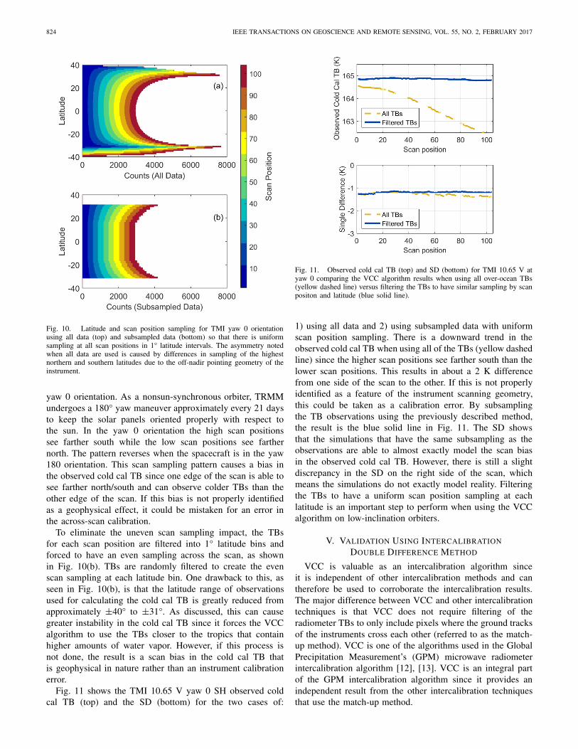
Fig. 11 shows the TMI 10.65 V yaw 0 SH observed coldcal TB (top) and the SD (bottom) for the two cases of:

Fig. 11. Observed cold cal TB (top) and SD (bottom) for TMI 10.65 V atyaw 0 comparing the VCC algorithm results when using all over-ocean TBs(yellow dashed line) versus filtering the TBs to have similar sampling by scanpositon and latitude (blue solid line).

1) using all data and 2) using subsampled data with uniformscan position sampling. There is a downward trend in theobserved cold cal TB when using all of the TBs (yellow dashedline) since the higher scan positions see farther south than thelower scan positions. This results in about a 2 K differencefrom one side of the scan to the other. If this is not properlyidentified as a feature of the instrument scanning geometry,this could be taken as a calibration error. By subsamplingthe TB observations using the previously described method,the result is the blue solid line in Fig. 11. The SD showsthat the simulations that have the same subsampling as theobservations are able to almost exactly model the scan biasin the observed cold cal TB. However, there is still a slightdiscrepancy in the SD on the right side of the scan, whichmeans the simulations do not exactly model reality. Filteringthe TBs to have a uniform scan position sampling at eachlatitude is an important step to perform when using the VCCalgorithm on low-inclination orbiters.

V. VALIDATION USING INTERCALIBRATION

DOUBLE DIFFERENCE METHOD

VCC is valuable as an intercalibration algorithm sinceit is independent of other intercalibration methods and cantherefore be used to corroborate the intercalibration results.The major difference between VCC and other intercalibrationtechniques is that VCC does not require filtering of theradiometer TBs to only include pixels where the ground tracksof the instruments cross each other (referred to as the match-up method). VCC is one of the algorithms used in the GlobalPrecipitation Measurement’s (GPM) microwave radiometerintercalibration algorithm [12], [13]. VCC is an integral partof the GPM intercalibration algorithm since it provides anindependent result from the other intercalibration techniquesthat use the match-up method.


TABLE V

INTERCALIBRATION RESULTS FOR TMI COMPARED WITH WINDSAT FORJULY 2005–JUNE 2006. THE VCC ALGORITHM SHOWS GOOD

AGREEMENT WITH THE OTHER TWO METHODS

The method of using the VCC algorithm for microwaveradiometer intercalibration is described in [4]. This section willshow that the VCC algorithm as an intercalibration methodcompares well with other intercalibration techniques.

A. VCC Comparison With Other Methods

Table V shows the results from Biswas et al. [14],Wilheit [15], and the VCC algorithm for TMI-WindSatdouble differences for July 2005–June 2006. The doubledifference (DD) and the TB at which the DD is cal-culated (Temp) are both shown. Biswas et al. [14] usethe match-up method of intercalibration with GDAS asinputs to the RTM. Wilheit [15] also uses the match-upmethod, but he computes the geophysical parameters for theRTM using a least squares fit method. Most of the channelsshow agreement among the three methods to within 0.2 K.One characteristic of the VCC algorithm that can be seenin Table V is that VCC typically derives a DD value at acolder TB than the match-up method. This is due to VCC onlyusing the coldest TBs with minimal water vapor, while theDD calculated from the match-up method typically includesTBs with higher levels of water vapor, which results inhigher TB values. Table V verifies that even though the VCCalgorithm uses a very different algorithm to calculate doubledifferences, it achieves similar results.

Since WindSat does not include a high-frequency(near 90 GHz) channel, the previous analysis could notcompare the performance of VCC at that frequency.Alsweiss et al. [16] calculated DDs for TMI compared withAMSR2 for January 2013–April 2013. Their results alongwith the VCC algorithm’s results are shown in Table VI.Alsweiss et al. [16] calculated DDs for AMSR2 separatedinto ascending and descending orbit nodes and the averageof these two nodes is reported here. Significant differencesbetween the two methods are seen for the 19 V, 19 H, and21 V channels. One explanation for this difference is the DDdependence on temperature. Alsweiss et al. [16] do not reporta temperature for their DDs, however, they do include a figure

TABLE VI

TMI-AMSR2 DOUBLE DIFFERENCES FOR JANUARY 2013–APRIL 2013[16] DO NOT INCLUDE A TEMPERATURE WITH THEIR

RESULTS SO THAT IS NOT INCLUDED HERE

illustrating the DD dependence on TB. Their analysis showsa strong DD dependence on TB for the 19 V, 19 H, and 21 Vchannels, and the VCC results at the reported temperatures lineup very closely with what they report. Discrepancies betweenthe two methods may also be explained by the lack of sufficientdata, since only four months are used to calculate the DD.The previous comparison with TMI-WindSat used a year ofdata.

The consistency of the results using the VCC DD with theother intercalibration methods shows that it is a valid andaccurate method to use for the intercalibration of spacebornemicrowave imagers.

B. Stability of VCC Double Difference

The previous section showed the results of the VCC DDmethod that were calculated by first finding the DD foreach month, and then taking the average of the monthlyDDs. This was done for ease of calculation since filteringthe data into monthly histograms is convenient. However,as shown in Section II, a month of data may not achievethe most stable cold cal TB for some channels. An analysisis done to see if averaging the monthly results gives themost stable DD, or if a different time period is moreappropriate.

The mean and standard deviation of the VCC DD iscalculated for one year of data, comparing weekly, monthly(shown in the previous section), and bimonthly filtering of thedata. As expected, the standard deviation of the DD decreasesas more data are used to calculate the DD. The mean, on theother hand, shows no significant change. The mean DD isthe quantity that is used for intercalibration purposes and thisanalysis shows that the time period used for calculation of theVCC DD does not impact the intercalibration.

VI. CONCLUSION

VCC for application to conical scanning microwave imagerswas presented. Modifications were made to the original algo-rithm to achieve a robust calibration reference for conical


scanners with frequencies from 6 to 90 GHz. The VCCalgorithm was divided into four steps and each was analyzedfor modification. These steps involve the calculation of thefirst-guess (Step 1), the TB range chosen from the first-guess to create a histogram subset of cold TBs (Step 2), theCDF range of the histogram subset (Step 3), and finally thepolynomial order used to derive the cold cal TB (Step 4). Thestandard deviation of simulated TBs across the radiometer scanwas used as a metric for stability since the simulated coldcal TB should be constant across the scan. The parametersin Steps 1–4 were varied and the values that resulted inthe lowest standard deviation across the scan were chosenfor the modified VCC algorithm. The modified algorithmwas shown to achieve a more stable calibration than theoriginal one that was designed for a nadir-viewing radiome-ter. Some channels were able to achieve a greater stabilitythan other channels due to the characteristics of individualchannels. The channels categorized in Group 1 (6.925 V/H,10.65 V/H, 18.7 V, and 36.5 V) are the least sensitive tosmall geophysical variations, resulting in a more stable cold calTB than those channels in Group 2 (18.7 H, 23.8 V, 36.5 H,and 89.0 V) and Group 3 (23.8 and 89.0 H). The Group 2and Group 3 channels require a data set with a longer timeperiod to reduce noise in the cold cal TB but are still unableto achieve the level of stability obtained with the Group 1channels.

The modified VCC algorithm was analyzed for dependenceon the geophysical and regional variability. It was found thatthe coldest TBs contributing to the calculation of the coldcal TB are determined largely by atmospheric water vapordistribution. Since the coldest TBs are determined by thewater vapor variability, the regions where the coldest TBsare produced can vary greatly with season. Any seasonaldependence in VCC is accounted for by taking the differencebetween the cold cal TB calculated from observations and thecold cal TB calculated from modeled TBs. This results in theSD that can be used as a relative calibration reference fora radiometer. The VCC SD was applied to TMI, a nonsun-synchronous orbiter in a shallow orbit inclination. It wasdetermined necessary to subsample the data to have consistentsampling by latitude across the scan to remove any samplingerror in the VCC SD.

Finally, VCC was shown to be an accurate microwaveintercalibration method by calculating the VCC DD andcomparing with other intercalibration methods. The VCC DDwas calculated for both WindSat and AMSR2 compared withTMI and in both the cases was shown to agree well withpreviously published results that use the match-up methodfor intercalibration. This demonstrated that the modified VCCalgorithm is a valid method to be used as a calibrationreference for conically scanning microwave imagers.

REFERENCES

[1] C. S. Ruf, “Detection of calibration drifts in spaceborne microwaveradiometers using a vicarious cold reference,” IEEE Trans. Geosci.Remote Sens., vol. 38, no. 1, pp. 44–52, Jan. 2000.

[2] C. S. Ruf, “Characterization and correction of a drift in calibration ofthe TOPEX microwave radiometer,” IEEE Trans. Geosci. Remote Sens.,vol. 40, no. 2, pp. 509–511, Feb. 2002.

[3] D. S. McKague, C. S. Ruf, and J. J. Puckett, “Beam spoiling correctionfor spaceborne microwave radiometers using the two-point vicariouscalibration method,” IEEE Trans. Geosci. Remote Sens., vol. 49, no. 1,pp. 21–27, Jan. 2011.

[4] R. A. Kroodsma, D. S. McKague, and C. S. Ruf, “Inter-calibrationof microwave radiometers using the vicarious cold calibration doubledifference method,” IEEE J. Sel. Topics Appl. Earth Observ. RemoteSens., vol. 5, no. 3, pp. 1006–1013, Jun. 2012.

[5] M. R. P. Sapiano, W. K. Berg, D. S. McKague, and C. D. Kummerow,“Toward an intercalibrated fundamental climate data record of theSSM/I sensors,” IEEE Trans. Geosci. Remote Sens., vol. 51, no. 3,pp. 1492–1503, Mar. 2013.

[6] K. Imaoka et al., “Global change observation mission (GCOM) formonitoring carbon, water cycles, and climate change,” Proc. IEEE,vol. 98, no. 5, pp. 717–734, May 2010.

[7] T. Meissner and F. J. Wentz, “The emissivity of the ocean surfacebetween 6 and 90 GHz over a large range of wind speeds and earthincidence angles,” IEEE Trans. Geosci. Remote Sens., vol. 50, no. 8,pp. 3004–3026, Aug. 2012.

[8] P. W. Rosenkranz, “Water vapor microwave continuum absorption:A comparison of measurements and models,” Radio Sci., vol. 33, no. 4,pp. 919–928, Jul./Aug. 1998.

[9] H. J. Liebe, P. W. Rosenkranz, and G. A. Hufford, “Atmospheric 60-GHzoxygen spectrum: New laboratory measurements and line parameters,”J. Quant. Spectrosc. Radiat. Transf., vol. 48, nos. 5–6, pp. 629–643,1992.

[10] CISL Data Support Section at the National Center forAtmospheric Research, Boulder, CO, USA. (Aug. 2014). U.S.National Centers for Environmental Prediction, Updated Daily:NCEP FNL Operational Model Global Tropospheric Analyses,Continuing From July 1999. Dataset ds083.2. [Online]. Available:http://dss.ucar.edu/datasets/ds083.2/

[11] R. A. Kroodsma, D. S. McKague, and C. S. Ruf, “Extension of vicariouscold calibration to 85–92 GHz for spaceborne microwave radiometers,”IEEE Trans. Geosci. Remote Sens., vol. 51, no. 9, pp. 4743–4751,Sep. 2013.

[12] T. Wilheit et al., “Intercalibrating the GPM constellation using the GPMmicrowave imager (GMI),” in Proc. IEEE Int. Geosci. Remote Sens.Symp. (IGARSS), Milan, Italy, Jul. 2015, pp. 5162–5165.

[13] A. Y. Hou et al., “The global precipitation measurement mis-sion,” Bull. Amer. Meteorol. Soc., vol. 95, no. 5, pp. 701–722,May 2014.

[14] S. K. Biswas, S. Farrar, K. Gopalan, A. Santos-Garcia, W. L. Jones,and S. Bilanow, “Intercalibration of microwave radiometer bright-ness temperatures for the global precipitation measurement mission,”IEEE Trans. Geosci. Remote Sens., vol. 51, no. 3, pp. 1465–1477,Mar. 2013.

[15] T. T. Wilheit, “Comparing calibrations of similar conically scanningwindow-channel microwave radiometers,” IEEE Trans. Geosci. RemoteSens., vol. 51, no. 3, pp. 1453–1464, Mar. 2013.

[16] S. O. Alsweiss, Z. Jelenak, P. S. Chang, J. D. Park, and P. Meyers,“Inter-calibration results of the Advanced Microwave ScanningRadiometer-2 over ocean,” IEEE J. Sel. Topics Appl. Earth Observ.Remote Ses., vol. 8, no. 9, pp. 4230–4238, Sep. 2015.

Rachael A. Kroodsma (S’09–M’14) received theB.S.E. degree in earth systems science and engi-neering, the M.S.E. degree in electrical engineering,and the Ph.D. degree in atmospheric, oceanic, andspace sciences from the University of Michigan,Ann Arbor, MI, USA, in 2009, 2013, and 2014,respectively.

She is currently a Post-Doctoral Associate withthe Earth System Science Interdisciplinary Center,University of Maryland, College Park, MD, USA.She is with the Precipitation Processing System at

NASA Goddard Space Flight Center, Greenbelt, MD, USA. As a memberof the Global Precipitation Measurement (GPM) inter-calibration workinggroup (XCAL), she works on developing inter-calibration techniques andmonitoring the calibration of the GPM constellation microwave radiometers.Her current research interests include microwave radiometer calibration andremote sensing of the atmosphere.


Darren S. McKague received the Ph.D. degree inastrophysical, planetary, and atmospheric sciencesfrom the University of Colorado, Boulder, CO, USA,in 2001.

He was a Systems Engineer at Ball Aerospace,Boulder, CO, USA, and Raytheon, Aurora, CO,USA, and a Research Scientist at Colorado StateUniversity, Fort Collins, CO, USA. He was involvedin remote sensing with an emphasis on the devel-opment of space-borne microwave remote sensinghardware, passive microwave calibration techniques,

and on mathematical inversion techniques for geophysical retrievals. He isan Associate Research Scientist with the Department of Climate and SpaceSciences and Engineering, University of Michigan, Ann Arbor, MI, USA.His experience with remote sensing hardware includes systems engineeringfor several advanced passive and active instrument concepts and the designof the calibration subsystem on the Global Precipitation Mission (GPM)Microwave Imager as well as the development of calibration and inter-calibration techniques for the GPM constellation. His algorithm experienceincludes the development of a near-real time algorithm for the joint retrievalof water vapor profiles, temperature profiles, cloud liquid water path, andsurface emissivity for the Advanced Microwave Sounding Unit at ColoradoState University, and the development of the precipitation rate, precipitationtype, sea ice, and sea surface wind direction algorithms for the risk reductionphase of the Conical scanning Microwave Imager/Sounder.

Christopher S. Ruf (S’85–M’87–SM’92–F’01)received the B.A. degree in physics from ReedCollege, Portland, OR, USA, and the Ph.D. degreein electrical and computer engineering from theUniversity of Massachusetts at Amherst, Amherst,MA, USA.

He was with Intel Corporation, Aloha, OR, USA,Hughes Space and Communication, El Segundo,CA, USA, the NASA Jet Propulsion Laboratory,Pasadena, CA, USA, and Pennsylvania State Uni-versity, State College, PA, USA. He is currently a

Professor of Atmospheric Science and Electrical Engineering at the Universityof Michigan, Ann Arbor, MI, USA, and a Principal Investigator of the CycloneGlobal Navigation Satellite System NASA Earth Venture mission. His currentresearch interests include GNSS-R remote sensing, microwave radiometry,atmosphere and ocean geophysical retrieval algorithm development, andsensor technology development.

Dr. Ruf is a member of the American Geophysical Union, the AmericanMeteorological Society, and the Commission F of the Union Radio Scien-tifique Internationale. He was the Editor-in-Chief of the IEEE TRANSAC-TIONS ON GEOSCIENCE AND REMOTE SENSING, and has served on theeditorial boards of Radio Science and the Journal of Atmospheric and OceanicTechnology. He has been a recipient of four NASA Certificates of Recognitionand seven NASA Group Achievement Awards, as well as the 1997 TGRS BestPaper Award, the 1999 IEEE Resnik Technical Field Award, the 2006 IGARSSBest Paper Award, and the 2014 IEEE GRS-S Outstanding Service Award.

Documents

816 IEEE TRANSACTIONS ON GEOSCIENCE AND …ktb.engin.umich.edu/...Kroodsma-etal_Vicarious-Cal-Conical-Imagers.pdf · Vicarious Cold Calibration for Conical ... VCC has been shown