THE PLUTOCRATIC BIAS IN THE CPI:

EVIDENCE FROM SPAIN

Javier Ruiz-Castillo

Dept. de Economıa, Universidad Carlos III de Madrid, Spain

Eduardo Ley

International Monetary Fund, Washington DC, U.S.A.

Mario Izquierdo

Fundacion de Estudios de Economıa Aplicada, Madrid, Spain

Abstract. We define the plutocratic bias as the difference between theinflation measured according to the current official CPI and a democraticindex in which all households receive the same weight. (i) We estimatethat during the 1990s the plutocratic bias in Spain amounts to 0.055 percent per year, or about one third of the classical substitution bias estimatedby the Boskin Commission for the U.S. (ii) We find that a 16-dimensionalcommodity space can be conveniently reduced to 3 dimensions, consistingof a luxury good and two necessities. The price behavior of these 3 goodsprovides a convincing explanation of the oscillations experimented by theplutocratic bias. (iii) Finally, the fact that the plutocratic bias is positiveduring this period, implies that the change in money income inequality isbetween 2 and 5 per cent greater than the change in real income inequality.We study the robustness of these results to the time period consideredand to the definition of the group index which serves as an alternative tothe CPI. We estimate that during the 1980s and the second part of the1970s in Spain, the plutocratic bias is 0.033 and 0.239 per cent per year,respectively.

Keywords. Consumer price index, cost-of-living index, aggregation, in-equality.

JEL Classification System. C43, D31, D63

Address. Javier Ruiz-Castillo, Departamento de Economıa, UniversidadCarlos III, c/ Madrid 126, 28903-Getafe, Madrid. Phone: +34-91-6249588. Email: jrc@eco.uc3m.es

1. INTRODUCTION

In all countries, the official CPI (Consumer Price Index), which is meant to be repre-

sentative for a certain reference population, is a fixed-weight price index. At least since

Konus (1924), economists have known that a fixed-weight CPI suffers from a “substitu-

tion bias” relative to a true cost-of-living index which, instead of maintaining constant

the budget shares of the households represented in the index, maintains constant their

living standards or welfare levels. But according to the review of the literature carried

out by a U.S. Senate Commission headed by Michael Boskin (Boskin et al., 1996), this

is not all that is wrong with the U.S. CPI elaborated by the BLS (Bureau of Labor

Statistics).

The Boskin Commission focused on five sources of bias in the CPI, all of which

are supposed to contribute to an overstatement of the true inflation in the cost of

living in the U.S.: (1) The substitution bias among commodities, or the “upper level

substitution” problem, causes an estimated upward bias of 0.15 per cent per year. (2)

The way elementary price quotations are aggregated within each geographic zone, or

the “lower level substitution” problem, is responsible for a bias of 0.25 per cent per year.

(3) Consumers adjust their behavior on where to buy in response to price differences

between the outlets which happen to be sampled by the BLS and other outlets which are

competing with them by lowering prices. The outlet substitution bias due to the failure

of the CPI to reflect this aspect of consumer behavior, is estimated at 0.10 per cent per

year. The last two sources of bias have to do with the alleged failure of the BLS (4) to

take fully into account the quality changes experienced in many sectors of the economy,

and (5) to introduce in a timely fashion the new products constantly appearing on the

market. These two sources together are supposed to cause a bias of 0.60 per cent per

year.

Thus, the Boskin Commission estimates that, on average, during the last few decades

the U.S. CPI has been overstating the inflation by 1.1 per cent per year. This bias

This research has profited from financial support of the Research Department of ”la Caixa”.

1

might seem small. However, when compounded over time, the implications for (i)

the public deficit created through an indexed budget, (ii) the wage bargaining process

and the determination of the nominal interest rates in the private sector, and (iii) the

measurement of the economic performance in real terms, are little short of catastrophic.1

Be this as it may, the fact is that the report has become already very influential.2 This

does not mean, of course, that it has escaped criticism. Some critics question the

Commission’s analysis of each and every one of the five sources of bias (Moulton et al.,

1998). Others point out toward neglected issues and, in particular, the scant attention

paid to distributional issues to which we now turn our attention —see, e.g., Pollak

(1998), Deaton (1998), and Madrick (1997).

In the CPI context, the issues raised by the heterogeneity of the population are

usually identified by asking “Whose cost-of-living index?,” a question which is seen to

contain three issues in Pollak (1998). “How many cost-of-living indexes?,” “Beer or

champagne?,” and “What type of group indexes?” The first issue refers to whether

we should have different indexes for different groups —rich and poor, elderly and non-

elderly, urban and rural, etc. The second issue refers to the selection of the appropriate

set of items, qualities and outlets that are to be reflected in the index.3

Assume that the population of households (individuals or consumers) for whom a

representative index must be constructed has been decided, and that a solution has been

found for the beer-vs-champagne issue. The third issue, which is the topic of this paper,

originates with the nature of the CPI as a group index. Given the commodity space

and a household budget survey representative of the reference population, we can use

1 For an evaluation of these sources of bias in the measurement of inflation through the official Spanishprice index and its implications for the Spanish economy, see Ruiz-Castillo et al. (1999b).

2 As Diewert (1998) puts it: “. . . with a total budget of $25,000, Boskin, Dulberger, Griliches, Gordonand Jorgenson have probably written the most important measurement paper of the century in termsof its impact: Every statistical agency in the world is revaluating its price measurement techniques asa direct result of their report and the widespread publicity it has received.”

3 Against the view of the Boskin Commission and Diewert (1995) that the “lower level substitution”problem is primarily a problem of choosing an appropriate formula for combining the prices of items,Pollak (1995, 1998) argues that it is primarily a problem of selecting the “items” to be priced, andreflects fundamental ambiguities in the meaning of “goods,” “commodities,” and “items” at theoreticaland empirical levels.

2

each household’s budget shares as the fixed weights for the construction of household-

specific price indexes. Since Prais (1958), we know that the CPI is the weighted average

of such individual price indexes with weights proportional to each household’s total

expenditures. Because richer households weigh more than poor ones, Prais baptized

the CPI as a plutocratic price index. The question is whether we can think of a better

alternative to this particular construction.4

In this paper, we defend that the so-called democratic index, in which all households

receive the same weight, is an option worth pursuing. Thus, we define the plutocratic

bias as the difference between the inflation measured according to the current official CPI

and a democratic index. We offer two reasons for being interested in such a concept.

In the first place, it is always interesting to know who suffers the greatest inflation:

those households with the largest total expenditures, or those at the bottom of the

distribution, in which case we would say that prices have behaved in an anti-rich or an

anti-poor manner, respectively. In the first (second) case we should expect that the mean

inflation weighted by the total household expenditures would be greater (smaller) than

the simple mean. Thus, the plutocratic bias would be positive or negative according

to whether prices have behaved in an anti-rich or in an anti-poor manner, respectively

—this idea can be traced back to Fry and Pashardes (1985).

In the second place, when two distributions of household expenditure, or income,

are expressed at constant prices using household-specific price indexes, the change in

nominal income inequality —which is the magnitude usually estimated in the empirical

literature— is seen to be equal to the change in real income inequality plus a price term

which captures the distributional impact of price changes.5 Knowledge of the sign of

the plutocratic bias takes us a long way in the direction of knowing the sign of the price

term. Thus, whether a given change in money income inequality is smaller (larger)

4 As pointed out by Pollak (1998), the first two issues are given a cursory treatment in footnote 2and page 71 of Boskin et al. (1996). The Boskin Commission never addresses the third issue directly,although Pollak selects some passages of its report which appear to reflect an implicit judgement thatthe CPI ought to be a plutocratic price index.

5 The idea that price movements should be included in intertemporal income inequality comparisonswas originally suggested by Iyengar and Battacharya (1965). Subsequently, in a social welfare con-text Muellbauer (1974) showed that under general assumptions on individual preferences real incomeinequality comparisons are not price independent.

3

than the socially relevant change in real income inequality depends to a large extent on

whether the plutocratic bias is positive (negative).

Nevertheless, the importance of this concept depends crucially on its empirical mag-

nitude. Our main result is that the plutocratic bias in Spain during the 1990s is equal

to 0.055 per cent per year —or about one third of the classical substitution bias es-

timated by the Boskin Commission for the U.S. Nonetheless, averaging magnitudes of

different signs underestimates the real importance of this bias. The bias in specific years

oscillates from a maximum of 0.150 to a minimum of −0.080 per cent per year. Inter-

estingly, neither the sign nor the magnitude of the bias in a given subperiod depends

on the magnitude of the inflation in that subperiod. Using the total expenditures elas-

ticities estimated in an Engel curve system, we find that a 16-dimensional commodity

space can be conveniently reduced to 3 dimensions, consisting of a luxury good and two

necessities. The price behavior of these 3 goods provides a convincing explanation of the

oscillations experimented by the plutocratic bias. Finally, the fact that the plutocratic

bias is positive, implies that the gap between the changes in nominal and real household

expenditures inequality during the 1990s is between 2 and 5 per cent, depending on the

inequality measure and the importance we give to the scale economies in consumption

within the household.

The paper studies the robustness of these results in two dimensions. In the first place,

we estimate the plutocratic bias for the 1980s and the second part of the 1970s in Spain.

We find that, on average, the bias is small in the first case and large in the second: 0.033

and 0.239 per cent per year, respectively.6 In the second place, we ask what would have

been the bias in the measurement of inflation if instead of using the plutocratic CPI we

were to use a group index equal to the weighted mean of the household-specific indexes

with weights proportional to the household size. We find that such a bias for the 1990s,

the 1980s and the second part of the 1970s would be equal to 0.088, 0.015 and 0.223

per cent per year, respectively.

6 The sign and the magnitude of the bias for these two periods are consistent with previous findingsabout the fact that the decrease in the real household’s total expenditures inequality is greater thanthe decrease in the money inequality —see Del Rıo and Ruiz-Castillo (1996), and Ruiz-Castillo andSastre (1999).

4

The rest of the paper is organized as follows. Section 2 presents the essentials on

individual and aggregate price indexes. Section 3 presents the empirical results on the

plutocratic bias in Spain during the 1990s, while Section 4 studies the implications

for total household expenditures inequality measurement. Section 5 is devoted to the

robustness of those results during previous periods, and the use of weighted group

indexes with weights proportional to household size. Section 6 summarizes and discusses

the political implications of our results in a heavily indexed economy.

2. INDIVIDUAL AND GROUP INDEXES

2.1. Individual Price Indexes

Let there be I goods and H households indexed by i = 1, . . . , I and h = 1, . . . , H,

respectively, and let q = (q1, . . . , qI) be a commodity vector. Each household h is

characterized by her total expenditures, xh, and her preferences represented by a utility

function, u = Uh(q). Assume that all households have the same preferences, so that

u = Uh(q) = U(q) for all h, and let c(u,p) be the cost function, which gives the

minimum cost of achieving the utility level u at prices p. Under general conditions, we

know that xh = c(U(qh),p), where qh is the utility-maximizing commodity vector at

prices p when the household expenditures are xh.

Consider two price vectors p0 and pt in periods 0 and t. A true or a Konus cost-of-

living index (COLI for short) which takes as its reference the utility level uh, is defined

as the ratio of the minimum cost of achieving that utility level at prices pt and p0, i.e.,

κ(pt,p0;uh) =c(pt, uh)c(p0, uh)

.

When the reference utility is the utility-maximizing level at prices p0, denoted by uh0 ,

we say that the COLI κ(pt,p0;uh0 ) = c(pt, uh0 )/c(p0, uh0 ) is a Laspeyres type index.

Given a reference commodity vector, qh, we can define a statistical price index (SPI)

as the ratio of the cost of acquiring qh at prices pt and p0,7

`(pt,p0; qh) =pt · qhp0 · qh

.

7 An SPI can also be written as a weighted average of individual-commodity indexes. Let whi0 be the

good-i household budget share at prices p0, i.e., whi0 = pi0qhi0/p0qh0 . Then we have that `(pt,p0; qh0 ) =∑

iwhi0(pit/pi0).

5

When qh = qh0 , the utility-maximizing consumption bundle at prices p0, we say that

the SPI `(pt,p0; qh0 ) = pt · qh0/p0 · qh0 is a Laspeyres type index.

A fundamental theorem in Konus (1924) establishes that, under general assumptions,

the Laspeyres SPI provides an upper bound to the Laspeyres COLI,

κ(pt,p0;uh0 ) ≤ `(pt,p0; qh0 ).

Equality is obtained when preferences are of the Leontief type, i.e., when there is no

substitution between goods.

2.2. The CPI

Define the vector of aggregate quantities bought in situation 0 by Q0 = (Q10, . . . , QI0),

where Qi0 =∑h q

hi0, and let Wi0 = pi0Qi0/p0 ·Q0. The aggregate Laspeyres SPI —for

period t based on period 0— is then defined as follows:

L(pt,p0; Q0) =∑i

Wi0pitpi0

=pt ·Q0

p0 ·Q0. (1)

However, the CPI actually computed by statistical agencies is not exactly an aggregate

price index of the type defined in equation (1). The reason is that individual behavior

is typically investigated by means of a household budget survey conducted in a period

τ prior to the index base period 0. As it is shown in the Appendix, the CPI based on

period 0 is an aggregate SPI defined by8

CPI(pt,p0; Qτ ) =L(pt,pτ ; Qτ )L(p0,pτ ; Qτ )

=pt ·Qτ

p0 ·Qτ. (2)

This is what the BLS calls a modified Laspeyres aggregate price index (Moulton, 1996).

What are the normative bases for such a construction? To answer this question we need

to define a set of household-specific modified Laspeyres price indexes:

cpi(pt,p0; qhτ ) =`(pt,pτ ; qhτ )`(p0,pτ ; qhτ )

=pt · qhτp0 · qhτ

.

8 Note that we could instead use average quantities, Qτ , with elements Qiτ = 1HQiτ , since the 1

Hterms in the numerator and denominator would cancel off. Hence the notion of the CPI being referredto an ‘average consumer.’

6

For each h, let uhτ = U(qhτ ). It is easy to see that the ratio of the corresponding

Laspeyres COLIs leads to what we can call a modified Laspeyres COLI:

κ(pt,pτ ;uhτ )κ(p0,pτ ;uhτ )

=c(pt, uhτ )c(p0, uhτ )

= κ(pt,p0;uhτ ).

Konus theorem assures that, for each h, `(p0,pτ ; qhτ )−κ(p0,pτ ;uhτ ) ≥ 0 and `(pt,pτ ; qhτ )−κ(pt,pτ ;uhτ ) ≥ 0, but it says nothing about the ratio of the Laspeyres indexes which

give rise to an individual CPI. However, the household budget survey collection pe-

riod τ is typically not far apart from the base year 0 of the CPI system. Thus, under

the assumption that the substitution bias `(p0,pτ ; qhτ ) − κ(p0,pτ ;uhτ ) is smaller than

`(pt,pτ ; qhτ ) − κ(pt,pτ ;uhτ ), we have that a household-specific CPI provides an upper

bound to a modified Laspeyres COLI. As shown in the Appendix,

CPI(pt,p0; Qτ ) =∑h

φh cpi(pt,p0; qhτ )

where φh = p0 · qhτ/p0 ·Qτ . Thus, only under the assumption that, for a sufficiently

large number of households,

cpi(pt,p0; qhτ ) =`(pt,pτ ; qhτ )`(p0,pτ ; qhτ )

≥ κ(pt,pτ ;uhτ )κ(p0,pτ ;uhτ )

= κ(pt,p0; uhτ ),

then the aggregate CPI provides an upper bound to a plutocratic-weighted mean of mod-

ified Laspeyres COLIs:9 CPI(pt,p0; Qτ ) ≥∑h φ

h κ(pt,p0; qhτ ). Otherwise it would

instead provide a lower bound. Nonetheless, the proximity of the theoretical construct

—i.e., a COLI— and the empirical counterpart —i.e., the CPI— constitutes a rather

remarkable situation.

9 In the democratic case, we have that 1H

∑h`(pt,p0; qhτ ) ≥ 1

H

∑hκ(pt,p0; qhτ ). Under the same

assumption, the simple mean of modified Laspeyres SPIs constitutes an upper bound to the simplemean of modified Laspeyres COLIs.

7

3. THE PLUTOCRATIC BIAS

3.1. The Data

In order to estimate the plutocratic bias defined below, we need to construct a series of

household-specific Laspeyres price indexes. For that purpose, we use the following two

pieces of publicly available information in Spain: the 1990–91 household-budget survey

(EPF) used to estimate the weights of the official CPI, and a set of price subindexes at

a certain level of spatial and commodity disaggregation.

The EPF (Encuesta de Presupuestos Familiares) collected by the Spanish statisti-

cal agency, INE (Instituto Nacional de Estadıstica), from April 1990 to March 1991,

is a household budget survey of 21,155 household sample points, representative of a

population of approximately 11 milllion households and 38 million persons occupying

residential housing in all of Spain, including the North African cities of Ceuta and

Melilla.

The INE collects elementary price indexes (denoted by Eijt in the Appendix) for a

commodity basket consisting of 471 items in each of the 52 provinces under the CPI

present system, based in 1992. For confidentiality reasons, the INE does not publish this

information at the maximum disaggregation level. Instead, it publishes on a monthly

basis price subindexes for the period January 1993 to January 1998 for a commodity

breakdown of 110 subclases, 57 rubricas, 33 subgrupos and 8 grupos at the national level,

the rubricas, subgrupos and grupos at the 18 Autonomous Community level, and the

subgrupos and grupos at the 52 province level.

For any commodity breakdown, it is possible to reconstruct the official CPI series

using an appropriately defined aggregate budget shares vector. Similarly, defining a

budget share vector for every household in the 1990–91 sample, we can obtain a series of

household-specific CPIs for any commodity breakdown. In principle, the only difference

between alternative specifications of the commodity space, is that the dispersion of

the set of individual CPIs should be greater the greater the disaggregation level of the

price information used in their construction. Unfortunately, in spite of using the same

informational basis as the INE —namely, the 1990–91 EPF— we find several small

discrepancies between our estimates of the aggregate budget share vectors and those

8

published by the INE —for the details, see Ruiz-Castillo et al. (1999b). Thus, the CPI

series which we can reconstruct vary slightly depending on the different commodity

breakdowns characterizing the price information we use. In Ruiz-Castillo et al. (1999b)

we find that the specification consisting of the 21 food rubricas at the Autonomous

Community level, and the 32 non-food subgrupos at the provincial level outperforms

the rest of the alternatives according to various statistical and economic criteria.

It should be emphasized that our series of household-specific price indexes defined

over this 53 commodity space differ from the series underlying the official CPI in two

ways. In the first place, there are a number of aspects in the official definition of total

household expenditures for which we believe there are superior alternatives. We refer to:

(i) the definition of housing expenditures for households occupying non-rental housing;

(ii) the inclusion of imputations for home production, wages in kind and subsidized

meals, and (iii) the estimation of annual food and drink expenditures using all the

available information on bulk purchases in the 1990–91 EPF. The joint impact of these

modifications is important: according to Ruiz-Castillo et al. (1999b), the official CPI

understates the true Spanish inflation from 1992 to January of 1998 in 0.241 per cent

per year.

In the second place, it should be noticed that the Spanish CPI is not the modified

Laspeyres price index defined in equation (2), which takes as a reference the mean

quantity vector actually acquired by the EPF households at the time they were inter-

viewed in the 1990–91 survey period. The reason is that the INE does not use the

adjustment factors Aijτ defined in the Appendix. Fortunately, Lorenzo (1998) provides

such factors for the 110 subclases at the national level. Using this information, for each

household h interviewed in a quarter τ during the 1990–91 period (τ = Spring, Sum-

mer, Autumn of 1990, and Winter of 1991), we construct a series of modified Laspeyres

SPIs, `(pt,p0; qhτ ), based on period 0 = Winter of 1991, which takes as a reference the

commodity vector qhτ actually acquired during the interview quarter τ :10

10 If we normalize this series at prices of period 0 = 1992, we can obtain the conceptually correctCPI, that is, `(pt,pτ ; qhτ )/`(p0,pτ ; qhτ ) = pt · qhτ /p0 · qhτ = CPIh(pt,p0; qhτ ). For the details of thisconstruction, see Ruiz-Castillo et al. (1999a). This series of modified Laspeyres price indexes is availableat http://www.eco.uc3m.es/investigacion/epf.html.

9

3.2. A Definition of the Plutocratic Bias

We will divide the period Winter 1991–January 1998 in the 7 subperiods shown on table

1 below. For each h we define the inflation (or deflation) caused by the evolution of

prices in a given subperiod by:

πht =`ht − `ht−1

`ht−1

The distribution of individual inflations in each subperiod is denoted by πππt = (π1t , . . . , π

Ht ).

For the entire period, we have ΠΠΠ = (Π1, . . . ,ΠH), where Πh = (`hT−1), where T = Jan98.

The aggregate inflation for the population as a whole according to the plutocratic scheme

is

PLUTt =∑h φ

h (`ht − `ht−1)∑h φ

h`ht−1

=∑h(φh`ht−1) (`ht − `ht−1)/`ht−1∑

h φh`ht−1

=∑h

ψht πht ,

where ψht = φh`ht−1/∑h φ

h`ht−1. For the democratic scheme,

DEMt =∑h `

ht − `ht−1∑h `

ht−1

=∑h

ξht πht ,

where ξht = `ht−1/∑h `

ht−1 —note that ψht is proportional to φhξht . Since `h0 = 1,

for the overall period from 0 to T the weights simplify to φh and 1H and we have

PLUT =∑h φ

h (`hT − 1), and DEM = 1H

∑h(`hT − 1). We define the plutocratic bias

in the measurement of inflation in subperiod t by Bt = PLUTt − DEMt, and for the

overall period by B = PLUT−DEM.11 Notice that, as pointed out in the Introduction,

if price changes in subperiod t (or for the entire period) are relatively more detrimental

to the rich, i.e., if πht (or Πh) are greater for the rich than for the poor households, then

we expect the plutocratic mean of individual inflations in the plutocratic case to be

greater than the democratic mean. That is, Bt or B are positive (negative) according

to whether the price change in the corresponding time interval is anti-rich (anti-poor).

3.3. The Main Findings

In the first two columns of Table 1 we show the plutocratic and the democratic means

of both ΠΠΠ and πππt. For comparative purposes with the measurement units used by the

11 Note that the inflation rate does not display temporal separability —i.e., the inflation for a givenperiod does not equal the sum of inflations for a partition of that period. If the inflation rate weredefined instead as the log price change, then temporal separabilty would hold but group separabilitywould be lost.

10

Boskin Commission, all figures are expressed in annual terms. Notice that the aggregate

inflation keeps decreasing over time, from a high 6.9 percentage points during the first

subperiod to a low 2.4 percentage points during 1997. In column 3 we measure the

plutocratic bias as the difference between the plutocratic and the democratic means

of distributions ΠΠΠ and πt. Note, however, that this summary for the whole period

understates the true importance of the plutocratic bias since the positive and negative

biases in various subperiods offset each other.

Table 1. The Plutocratic Bias During the 1990s(In Percent Per Year)

Inflation

t Subperiods Plutocratic Democratic Plutocratic bias

1 Winter 91 to 1992 6.989 6.911 0.078

2 1992 to Jan 1993 5.394 5.244 0.150

3 Jan 93 to Jan 94 5.271 5.165 0.105

4 Jan 94 to Jan 95 4.621 4.701 -0.080

5 Jan 95 to Jan 96 4.079 4.130 -0.050

6 Jan 96 to Jan 97 3.180 3.090 0.090

7 Jan 97 to Jan 98 2.494 2.369 0.125

Winter 91 to Jan 98 4.632 4.577 0.055

The main findings are the followings three: (1) For the period as a whole, B is

positive and equal to 0.055 per cent per year. This is, approximately, one third of the

substitution bias estimated by the Boskin Commission for the U.S. economy, which is

equal to 0.15 per cent per year. (2) Price behavior is not uniform over the entire period:

Bt is negative during 1994 and 1995, indicating that during these two years prices have

caused relatively more damage to the poor than to the rich households. (3) Neither the

sign nor the magnitude of Bt in a given period depends on whether inflation is large or

small during that period.

3.4. An Economic Interpretation

Which goods are primarily consumed by the poor or the rich households? To answer

this question, we must begin by recognizing the fact that, in a heterogeneous world,

total expenditures of households with different characteristics are not directly compa-

rable. Following Buhmann et al. (1988) and Coulter et al. (1992a, 1992b), we adopt

an equivalence scale model in which scale economies in consumption depend only on

11

household size, sh, and adjusted total household expenditures are defined by

yh =xh

(sh)θ, θ ∈ [0, 1] (3)

When θ = 0, adjusted expenditures coincide with unadjusted household expenditures,

while if θ = 1, it becomes per capita household expenditures. Taking a single adult as

the reference type, the expression sθ can be interpreted as the number of equivalent

adults in a household of size s. Thus, the greater the equivalence elasticity θ, the

smaller the scale economies in consumption or, in other words, the larger the number

of equivalent adults.

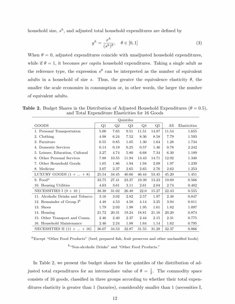
Table 2. Budget Shares in the Distribution of Adjusted Household Expenditures (θ = 0.5),and Total Expenditure Elasticities for 16 Goods

Quintiles

GOODS Q1 Q2 Q3 Q4 Q5 All Elasticities

1. Personal Transportation 5.00 7.65 9.51 11.51 14.87 11.54 1.655

2. Clothing 4.98 6.24 7.52 8.36 8.58 7.79 1.593

3. Furniture 0.55 0.85 1.05 1.30 1.64 1.28 1.734

4. Domestic Services 0.14 0.19 0.25 0.57 1.46 0.78 2.242

5. Leisure, Education, Cultural 3.27 4.74 5.80 6.68 7.34 6.30 1.189

6. Other Personal Services 7.88 10.55 11.94 13.43 14.71 12.92 1.340

7. Other Household Goods 1.65 1.86 1.94 1.94 2.09 1.97 1.239

8. Medicine 2.07 2.37 2.65 2.65 2.76 2.62 1.253

LUXURY GOODS (1 + ... + 8) 25.54 34.45 40.66 46.44 53.45 45.20 1.451

9. Fooda 33.75 27.41 23.37 19.39 13.23 19.69 0.566

10. Housing Utilities 4.63 3.61 3.11 2.61 2.04 2.74 0.482

NECESSITIES I (9 + 10 ) 38.38 31.02 26.48 22.0 15.27 22.43 0.555

11. Alcoholic Drinks and Tobacco 3.16 3.02 2.82 2.57 1.97 2.48 0.847

12. Remainder of Group Ib 4.48 4.53 4.58 4.14 3.25 3.94 0.811

13. Shoes 1.79 2.03 1.98 1.95 1.61 1.82 1.097

14. Housing 21.72 20.31 19.24 18.81 21.16 20.20 0.874

15. Other Transport and Comm. 2.46 2.40 2.37 2.44 2.15 2.31 0.775

16. Household Maintenance 2.46 2.24 1.88 1.64 1.14 1.62 0.795

NECESSITIES II (11 + ... + 16) 36.07 34.53 32.87 31.55 31.28 32.37 0.866

aExcept “Other Food Products” (beef, prepared fish, fruit preserves and other unclassified foods)

b“Non-alcoholic Drinks” and “Other Food Products.”

In Table 2, we present the budget shares for the quintiles of the distribution of ad-

justed total expenditures for an intermediate value of θ = 12 . The commodity space

consists of 16 goods, classified in three groups according to whether their total expen-

ditures elasticity is greater than 1 (luxuries), considerably smaller than 1 (necessities I,

12

dominated by Food expenditures), or weakly smaller than 1 (necessities II, dominated

by Housing expenditures). The total expenditure elasticities are estimated at the mean

of the variables in the following system of Engel-curve regressions:

whi = αi + βi ln(yh) + γizh + εhi , i = 1, . . . , 16,

where: εhi is an error term; yh = xh/√sh is total household expenditures adjusted for

household size with parameter θ = 12 ; and zh is a vector of household characteristics

including (i) demographic variables (household size and composition, the household

head’s age and age squared), (ii) socioeconomic variables (number of income earners,

educational level and socioeconomic category of the household head, educational level

and labor status of the spouse, number of dwellings and characteristics of the resi-

dential unit), as well as (iii) seasonal and geographic variables (municipality size and

Autonomous Community of residence). In Figure 1 we display the joint distribution of

the individual budget shares for these three goods and the logarithm of the adjusted to-

tal household expenditures,12 the last panel shows the estimated Engel curves (trimming

the 1 percent tails off the support of the adjusted household expenditures).

[Insert Figure 1]

Intuitively, the evolution of prices would tend to damage to relatively greater extent

the richer households over the poorer ones according to whether the luxury good or the

necessities experience the greatest relative increase. For the entire period, the inflation

experienced by the luxury good and the two necessities are 31.59, 21.08, and 38.46 index

points, respectively. In Figure 2 we represent the evolution of the inter-annual inflation

of the three goods in relation to the general inflation as well as the inter-annual Bt, t =

January 1992,. . .,January 1998.

[Insert Figure 2]

In spite of the fact that the second necessity shows the stronger price growth, the

behavior of the luxury good and the first necessity is the main explanatory force behind

12 The boxplots on the top margins show the 1, 25, 50, 75 and 99 percentiles.

13

the positive sign of the plutocratic bias. To test this idea, we run a regression of the inter-

annual (January to January) plutocratic bias Bt, from t = January 1992,. . ., January

1998, on the corresponding monthly inter-annual price subindexes for the 3 goods and

a constant. The results, with robust t-ratios in parentheses (generalized least-squares

and Cochrane-Orcutt regressions yield identical results), are the following:

Bt = 0.025 + 0.050Lt − 0.056NIt − 0.0043NIIt R2 = 0.96

(1.80) (9.95) (−42.14) (−0.75)

All the coefficients have the expected sign —although the one corresponding to Necessi-

ties II (NII) is not statistically significant— and the results corroborate the explanatory

power of the Luxury good (L) and Necessities I (NI).

4. THE IMPLICATIONS FOR INEQUALITY MEASUREMENT

4.1. The Change in Money and Real Inequality

Let us assume that we want to compare the household income or expenditures distri-

butions in two different time periods, x0 = (x10, . . . , x

H0 ) and xt = (x1

t , . . . , xH′t ), with

H ′ not necessarily equal to H. Let p0 and pt be the price vectors in the two situations.

For each h, we can express the household’s total expenditures in situation 0 at prices

pt, xh0,t, by multiplying her original money income in period 0, xh0 , by an SPI of the

Laspeyres type:

xh0,t = xh0 `(pt,p0; qh0 ) = p0 · qh0pt · qh0p0 · qh0

= pt · qh0 .

For any H ≥ 2, let I : <H 7→ < be any convenient inequality index satisfying

continuity, S-concavity, scale independence and replication population invariance. The

change in money income inequality, ∆M , can be expressed as the sum of two terms:

∆M = I(xt)− I(x0) = [I(xt)− I(x0,t)] + [I(x0,t)− I(xt)] = ∆R+ ∆P, (4)

where ∆R = I(xt)−I(x0,t) is the change in real income inequality and ∆P = I(x0,t)−I(xt) captures the distributional impact of price changes on inequality measurement

according to the households’ preferences at period 0.13 ¿From a social point of view, we

13 We could have expressed the distribution in situation t at prices p0 by using an appropriate Paasschetype price index. In this case, ∆P = I(xt) − I(xt,0) would have measured the distributional impactof price changes according to the households’ preferences at t.

14

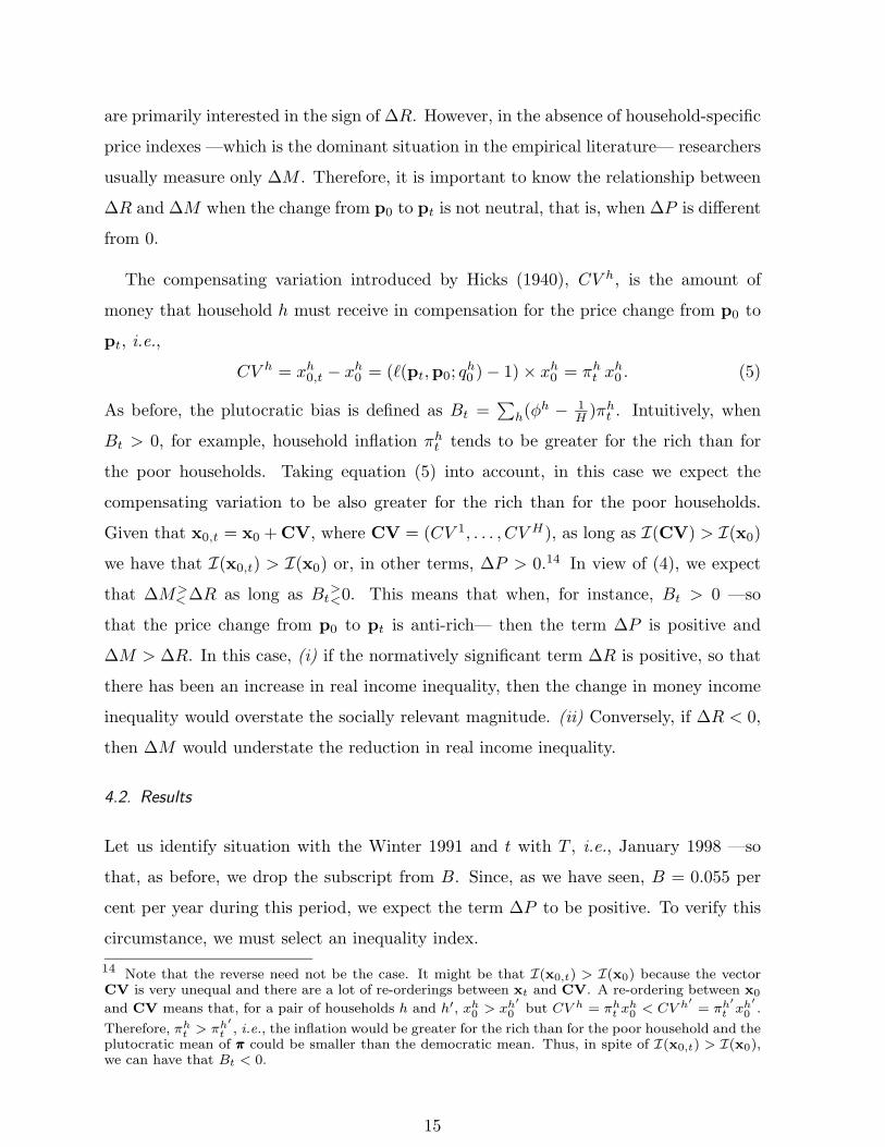
are primarily interested in the sign of ∆R. However, in the absence of household-specific

price indexes —which is the dominant situation in the empirical literature— researchers

usually measure only ∆M . Therefore, it is important to know the relationship between

∆R and ∆M when the change from p0 to pt is not neutral, that is, when ∆P is different

from 0.

The compensating variation introduced by Hicks (1940), CV h, is the amount of

money that household h must receive in compensation for the price change from p0 to

pt, i.e.,

CV h = xh0,t − xh0 = (`(pt,p0; qh0 )− 1)× xh0 = πht xh0 . (5)

As before, the plutocratic bias is defined as Bt =∑h(φh − 1

H )πht . Intuitively, when

Bt > 0, for example, household inflation πht tends to be greater for the rich than for

the poor households. Taking equation (5) into account, in this case we expect the

compensating variation to be also greater for the rich than for the poor households.

Given that x0,t = x0 + CV, where CV = (CV 1, . . . , CV H), as long as I(CV) > I(x0)

we have that I(x0,t) > I(x0) or, in other terms, ∆P > 0.14 In view of (4), we expect

that ∆M><∆R as long as Bt><0. This means that when, for instance, Bt > 0 —so

that the price change from p0 to pt is anti-rich— then the term ∆P is positive and

∆M > ∆R. In this case, (i) if the normatively significant term ∆R is positive, so that

there has been an increase in real income inequality, then the change in money income

inequality would overstate the socially relevant magnitude. (ii) Conversely, if ∆R < 0,

then ∆M would understate the reduction in real income inequality.

4.2. Results

Let us identify situation with the Winter 1991 and t with T , i.e., January 1998 —so

that, as before, we drop the subscript from B. Since, as we have seen, B = 0.055 per

cent per year during this period, we expect the term ∆P to be positive. To verify this

circumstance, we must select an inequality index.

14 Note that the reverse need not be the case. It might be that I(x0,t) > I(x0) because the vectorCV is very unequal and there are a lot of re-orderings between xt and CV. A re-ordering between x0

and CV means that, for a pair of households h and h′, xh0 > xh′

0 but CV h = πht xh0 < CV h

′= πh

′t x

h′0 .

Therefore, πht > πh′t , i.e., the inflation would be greater for the rich than for the poor household and the

plutocratic mean of πππ could be smaller than the democratic mean. Thus, in spite of I(x0,t) > I(x0),we can have that Bt < 0.

15

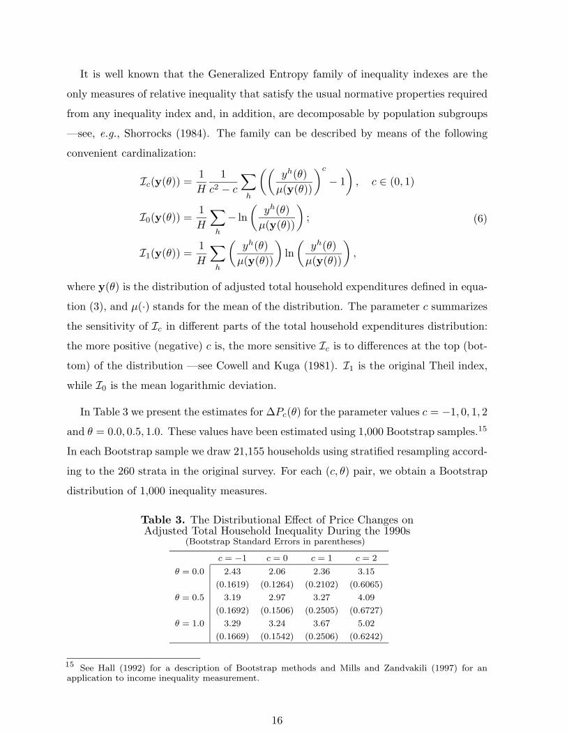
It is well known that the Generalized Entropy family of inequality indexes are the

only measures of relative inequality that satisfy the usual normative properties required

from any inequality index and, in addition, are decomposable by population subgroups

—see, e.g., Shorrocks (1984). The family can be described by means of the following

convenient cardinalization:

Ic(y(θ)) =1H

1c2 − c

∑h

((yh(θ)µ(y(θ))

)c− 1), c ∈ (0, 1)

I0(y(θ)) =1H

∑h

− ln(

yh(θ)µ(y(θ))

);

I1(y(θ)) =1H

∑h

(yh(θ)µ(y(θ))

)ln(

yh(θ)µ(y(θ))

),

(6)

where y(θ) is the distribution of adjusted total household expenditures defined in equa-

tion (3), and µ(·) stands for the mean of the distribution. The parameter c summarizes

the sensitivity of Ic in different parts of the total household expenditures distribution:

the more positive (negative) c is, the more sensitive Ic is to differences at the top (bot-

tom) of the distribution —see Cowell and Kuga (1981). I1 is the original Theil index,

while I0 is the mean logarithmic deviation.

In Table 3 we present the estimates for ∆Pc(θ) for the parameter values c = −1, 0, 1, 2

and θ = 0.0, 0.5, 1.0. These values have been estimated using 1,000 Bootstrap samples.15

In each Bootstrap sample we draw 21,155 households using stratified resampling accord-

ing to the 260 strata in the original survey. For each (c, θ) pair, we obtain a Bootstrap

distribution of 1,000 inequality measures.

Table 3. The Distributional Effect of Price Changes onAdjusted Total Household Inequality During the 1990s

(Bootstrap Standard Errors in parentheses)

c = −1 c = 0 c = 1 c = 2

θ = 0.0 2.43 2.06 2.36 3.15

(0.1619) (0.1264) (0.2102) (0.6065)

θ = 0.5 3.19 2.97 3.27 4.09

(0.1692) (0.1506) (0.2505) (0.6727)

θ = 1.0 3.29 3.24 3.67 5.02

(0.1669) (0.1542) (0.2506) (0.6242)

15 See Hall (1992) for a description of Bootstrap methods and Mills and Zandvakili (1997) for anapplication to income inequality measurement.

16

For every θ, the increase in income inequality is slightly greater for c = −1 and,

above all, for c = 2. This means that prices have affected primarily households at both

ends of the distribution and, above all, to those at the upper tail. On the other hand,

for every c, ∆Pc(θ) increases slightly as θ increases, that is, as the importance of scale

economies diminishes. At any rate, we find that, as expected, ∆Pc(θ) > 0 for all c

and θ and, in view of the standard errors, this increase in inequality is statistically

significant. Thus, because prices have behaved in an anti-rich manner during 1991–

1998, we conclude that the inequality of the 1990–91 adjusted household expenditures

inequality is between 2 and 5 per cent greater in January 1998 than in the Winter

of 1991. Assume that we have data on household expenditures in 1998 and that the

change in money household expenditures inequality is to be equal to 10 per cent, for

example. According to equation (4), our results on ∆Pc(θ) imply that the increase in real

household expenditures inequality would be only between 5 and 8 per cent depending

on the values of θ and c. If the change in money household expenditures inequality were

to be equal to −10 per cent, then the decrease in real household expenditures inequality

would be 12 or 15 per cent.

5. ROBUSTNESS

5.1. The Time Period

In this subsection we study the robustness of our results on the B trend in two different

directions. In the first place, we consider the period covered by the two previous Spanish

CPI systems, which run from August 1985 to December 1992 (base year = 1983) , and

from January 1977 to July 1985 (base year = 1976), respectively. The EPFs which

serve to estimate the official weights were conducted from April 1980 to March 1981,

and from July 1973 to June 1974, respectively. These are household budget surveys

strictly comparable to the 1990–91 EPF, containing 23,972 and 24,151 household sample

units, representative of, approximately, a population of 10 or 9 million households and

37 or 34 million persons in 1980–81 or 1973–74. In this case, we do not have reasons

to depart from the official definition of total household expenditures, but we must

take into account that, as before, the Spanish CPI is not a modified Laspeyres price

index. We construct two series of appropriate household-specific price indexes with the

17

information provided by: (i) the 1980-81 and 1973-74 EPFs; (ii) the official monthly

price information for 58 and 57 rubricas at the national level in the 1983 and 1976

bases, respectively, and (iii) a series of adjustment factors for 60 goods at the national

level provided by Catasus et al. (1986) for the first period, and for only 5 goods at the

national level provided by Garcıa Espana and Serrano (1980) for the second period.16

For the 1980s, we base the individual modified Laspeyres price indexes at Winter

1981, and distinguish between the following nine subperiods: 1) From Winter 1981 to

1983, the base year of the CPI system; 2) from 1983 to December 1984; and 3) - 9) from

r to r + 1, where r = December 1984,. . .,December 1990. For the second part of the

1970s, we base the individual modified Laspeyres price indexes at the midpoint of 1973

and 1974, and distinguish between the following six subperiods: 1) From the 1973-1974

to 1976, the base year of the CPI system; 2) from 1976 to December 1977; and 3) -

6) from r to r + 1, where r = December 1977,. . ., December 1980. The results on the

plutocratic bias in the measurement of inflation for these two periods are presented on

Tables 4 and 5.

Table 4. The Plutocratic Bias During the 1980s(In Percent Per Year)

Inflation

t Subperiods Plutocratic Democratic Plutocratic bias

1 Winter 81 to 1983 13.002 12.886 0.116

2 1983 to December 1984 9.484 9.655 -0.171

3 1985 7.782 7.857 -0.075

4 1986 8.230 8.420 -0.189

5 1987 4.587 4.292 0.295

6 1988 5.866 5.956 -0.089

7 1989 6.922 6.962 -0.040

8 1990 6.641 6.474 0.167

9 1991 5.604 5.350 0.254

Winter 81 to Winter 91 8.557 8.524 0.033

The first thing to notice is that the Spanish inflation during the 1970s and 1980s is

considerably greater than during the 1990s. However, as before, there is no relationship

16 For the 1980s, we had to work with a set of 52 goods which constitute the minimum commondenominator between the 58 official rubricas and the 60 goods in Catasus et al. (1986). For the 1970s,the minimum common denominator is given by the 5 goods in Garcıa Espana and Serrano (1980). Forthe details of these constructions, see Ruiz-Castillo et al. (1999a). Both series of modified Laspeyresprice indexes are available at http://www.eco.uc3m.es/investigacion/epf.html.

18

Table 5. The Plutocratic Bias From 1973–74 to Winter 1981(In Percent Per Year)

Inflation

t Subperiods Plutocratic Democratic Plutocratic bias

1 1973–74 to 1976 16.869 16.816 0.053

2 1976 to December 1977 23.024 22.497 0.527

3 1978 16.529 16.246 0.283

4 1979 15.523 14.806 0.717

5 1980 15.311 15.323 -0.012

6 1981 14.541 14.578 -0.037

1973–74 to Winter 81 17.746 17.506 0.239

between the size of the aggregate inflation in a given subperiod and the sign or the

magnitude of the plutocratic bias. As far as the 1980s is concerned, from 1983 to 1986

and from 1988 to 1989, Bt < 0. The sum of these magnitudes is more than offset by

the anti-rich price behavior during the remaining 3 subperiods. Thus, for the 1980s we

observe that B = 0.033 per cent per year, a positive bias smaller than what we saw for

the 1990s. However, from 1973-74 to the Winter of 1991, the plutocratic bias is always

positive and reaches very high annual maxima from 1976 to 1979. For the period as a

whole, B = 0.239 per cent per year, a bias whose size is equal to the sum of the classical

substitution bias and the outlet bias according to the Boskin Commission.

To appreciate the variability of the plutocratic bias during the entire period consid-

ered in this paper, Figure 3 shows the evolution of the inter-annual (month to month)

Bt, t = January 1977, . . . , January 1998, as well as the inter-annual inflation rate. Re-

gressing the bias in absolute value against inflation yields a nonsignificant coefficient

(0.005 with a standard error of 0.006, using generalized least squares correcting for

autocorrelation).

[Insert Figure 3]

These results can be related to those obtained in previous papers about the distri-

butional impact of price changes on household expenditures inequality measurement,

where household expenditures are defined as total household expenditures net of the

acquisition of some durables but inclusive of a number of expenditures which, although

not included in the CPI definition, we believe are part of the best possible approximation

to current consumption of private goods and services using the information available

in the EPF. Using the inequality index I1(·) defined in equation (6), Ruiz-Castillo and

19

Sastre (1999) point out that the term ∆P in equation (4) is almost 5 times greater

for the second part of the 1970s than for the 1980s. As a matter of fact, Del Rıo and

Ruiz-Castillo (1996) reports that although the Lorenz curve of the 1980-81 adjusted

household expenditures distribution at Winter 1981 prices dominates in a numerical

sense the Lorenz curve of that same distribution at Winter 1991 prices, from a statisti-

cal point of view both distributions are indistinguishable, so that the distributional role

of prices during the 1980s is essentially neutral. Nevertheless, for the 1973-74 to Winter

1981 period as a whole, Ruiz-Castillo and Sastre (1999) find that the decrease in real

household expenditures inequality —which is equal to 27 per cent— is 37.7 per cent

greater than the decrease in nominal household expenditures inequality; that is to say,

during this period the distributional impact of price changes on inequality measurement

is very important.

5.2. The Aggregation Scheme

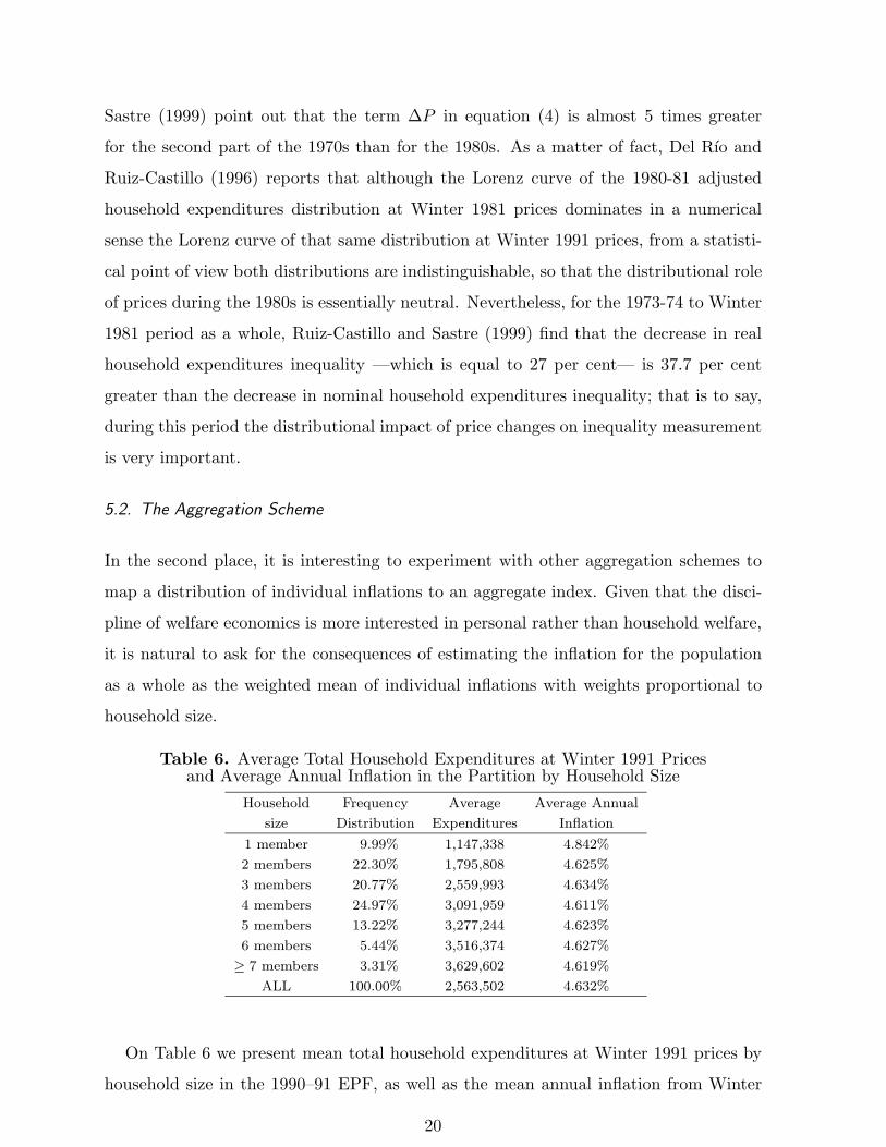
In the second place, it is interesting to experiment with other aggregation schemes to

map a distribution of individual inflations to an aggregate index. Given that the disci-

pline of welfare economics is more interested in personal rather than household welfare,

it is natural to ask for the consequences of estimating the inflation for the population

as a whole as the weighted mean of individual inflations with weights proportional to

household size.

Table 6. Average Total Household Expenditures at Winter 1991 Pricesand Average Annual Inflation in the Partition by Household Size

Household Frequency Average Average Annual

size Distribution Expenditures Inflation

1 member 9.99% 1,147,338 4.842%

2 members 22.30% 1,795,808 4.625%

3 members 20.77% 2,559,993 4.634%

4 members 24.97% 3,091,959 4.611%

5 members 13.22% 3,277,244 4.623%

6 members 5.44% 3,516,374 4.627%

≥ 7 members 3.31% 3,629,602 4.619%

ALL 100.00% 2,563,502 4.632%

On Table 6 we present mean total household expenditures at Winter 1991 prices by

household size in the 1990–91 EPF, as well as the mean annual inflation from Winter

20

1991 to January 1998 for that same partition. As in the majority of other countries, we

observe a positive association between total expenditures and household size. Therefore

weighting household inflation by household size should have a similar effect, although

of a lesser magnitude, than weighting directly by total household expenditures as in the

plutocratic scheme. On the other hand, the fact that 2, 4 and more member households

have a mean annual inflation below the population as a whole works in the opposite

direction. The end result is that the new bias —defined as the difference between the

plutocratic and the household size weighted mean— is equal to 0.088 per cent per year.

That this figure is greater than the previously estimated of 0.055 per cent per year

for the plutocratic bias, indicates that during this period the second factor has had a

greater impact than the first one.

The same computations for the 1980s and 1970s lead to an estimate of 0.015 and

0.223 for the new bias versus a plutocratic bias of 0.033 and 0.239, respectively. The

fact that the new bias is smaller than the plutocratic bias indicates that the positive

association between total household expenditures and household size dominates the size

of the new bias during these two periods.

6. CONCLUSIONS

In a country like Spain, a commodity basket of 471 goods is priced in each of the 52

provinces in order to construct the set of elementary price indexes which form the core of

the current 1992 CPI system. We have been able to work in a 53 dimensional commodity

space, consisting of the 21 food rubricas at the 18 Autonomous Community level, and the

32 non-food subgrupos at the 52 province level. For such a commodity breakdown, we

construct 21,155 household-specific Laspeyres price indexes representative of a 1990–

91 population of about 11 million households. Because of the fixed-weight nature of

our construction, the individual inflation variation we observe during the Winter 1991-

January 1998 period is the consequence of the price variation publicly disseminated by

the INE in this 53 commodity space.

How can we grasp the distributional consequences of such a complex multidimensional

process? In this paper we propose a procedure which combines three elements. In the

first place, whether price behavior in a given period hurts relatively more the rich or the

21

poor households can be expressed in terms of a single scalar: the so-called plutocratic

bias, incurred when we measure inflation using the current plutocratic CPI instead of

using an alternative group index in which all households weight equally. In the second

place, the estimation of an Engel curve system in a 16 goods commodity space, allows

us to reduce the size of the price universe to only three dimensions: a luxury good

and two necessities with considerably different total expenditures elasticities. Price

behavior at this level provides an intelligible explanation of the sign and magnitude of

the plutocratic bias. Finally, the change in money income inequality —which is the

only magnitude usually estimated in the empirical literature on income inequality— is

seen to be equal to the change in real income inequality —which is the socially relevant

magnitude— and a price term which captures the distributional impact of price changes

according to consumers’ preferences as manifested via their budget share vectors in a

given moment in time. The price term, and hence the gap between the change in money

and real income inequality, depends on the size and magnitude of the plutocratic bias.

Knowing the plutocratic bias is also important for two other topics in positive eco-

nomics. On one hand, in Spain —like in many other countries— the CPI is not really a

modified Laspeyres price index. Thus, one can define a “Laspeyres bias” as the differ-

ence between measuring inflation using an appropriate Laspeyres type index or using the

CPI actually constructed in these countries. As shown in Ruiz-Castillo et al. (1999d),

the sign of the plutocratic bias determines the sign of the Laspeyres bias. On the other

hand, recent theoretical results have opened up the way to the possibility of estimating

the classical upper level substitution bias in the CPI as the difference between the infla-

tion measured according to two readily computable statistical price indexes: a Laspeyres

price index, and a Tornquist one for which we only need to observe consumer choices

during the two periods under comparison. In Ruiz-Castillo et al. (1999e) we show how

the knowledge of the sign of the plutocratic bias helps us to overcome some difficulties

which arise when we attempt to apply this idea in practice.

But beyond all of the above measurement issues, what are the political consequences

of our research? The first question we need to rise is how should we adjust our income

taxes and public transfers annually. At this moment, we do not have anything to add

to the arguments offered by others.17 But we should recognize that, in most countries,

17 See Triplett (1983), Fry and Pashardes (1985), Griliches (1995), and Pollak (1998) and, in connection

22

income taxes, public pensions, other public transfers, and minimum wages are revised

in terms of a plutocratic CPI. Why should we follow a dollar rather than a household

or a personal logic in this matter? Perhaps because both people and experts believe

that the CPI represents an “average consumer.” However, when in an important but

unpublished paper Muellbauer (1976a) asked for the consumer whose budget shares are

equal to the official CPI aggregate weights, he answered that in the UK this consumer

occupied the 71 percentile in the household expenditures distribution.18 At any rate,

indexing by the current CPI has the following perverse effects which, in our opinion,

have not been sufficiently emphasized before: when prices behave in a anti-poor (anti-

rich) way, i.e., when the plutocratic bias is negative (positive), then we revise public

programs, which primarily benefit the poor, below (above) what would be the case with

a democratic group index. Similarly, if the plutocratic bias is negative (positive), then

direct tax revenues would be larger (smaller) than what would be the case under the

democratic alternative.

From this point of view, the current plutocratic formula can be conceptually critized.

Admittedly, this issue would be more important the greater the size of the plutocratic

bias (and perhaps, depending on the sign of the bias). In the Spanish case, we have

shown that this bias: (i) has had a positive sign over an extended period of time, (ii)

presents a rather unstable pattern over the short run, and (iii) has had a considerable

size during certain periods of time. There is relatively little information on this issue in

other countries,19 in particular in underdeveloped countries where the relative price of a

to the poverty line, see the National Research Council (1995).

18 See Muellbauer (1975, 1976b) for the theoretical basis of this work. For the U.S. in 1990, Deaton(1998) estimates that this consumer occupies the 75 percentile. In our case, we have simply computedthe location of Spanish consumers who have an inflation in a 5 per cent interval of the official oneduring the 1990s; the answer is that their mean adjusted household expenditures is in the 61 percentileof such distribution.

19 For the U.K., Carruthers et al. (1980) indicate that from January 1975 to January 1979 the demo-cratic index has increased by around 0.1 per cent per year faster than the official CPI; Fry and Pashardes(1985) obtain also that from 1974 to 1982 the plutocratic bias was negative; for 1975-76, Deaton andMuellbauer (1980) report that the inflation rate for the poor was around two points higher than for therich; however, Crawford (1996) finds that, between 1979 and the end of 1992, inflation for richer house-holds was 0.16 percentage points higher than the average for all households. For the U.S., Kokowski(1987) finds that from 1972 to 1980 the democratic and the plutocratic Laspeyres indexes are ratherclose in value for most demographic groups but, in general, the first measure exceeds its counterpartby 1 to 3 index points; Garner et al. (1999) find evidence that the plutocratic bias during the 1980s is

23

few staples may cause havoc in the standard of living of the majority of the population.

In our opinion, it is advisable to estimate the plutocratic bias on a regular basis. For

this and other purposes, we recommend that statistical agencies in charge of the CPI

compute and make available, at least annually, a set of household-specific price indexes.

This idea has the following four advantages:

1. We expect that the farther down we go towards the elementary price level, the greater

will be the dispersion of the distribution of household-specific price indexes. How-

ever, we would also expect a larger number of zero expenditures in most households.

Therefore, there are advantages and disadvantages in enlarging the commodity space.

Given that, for confidentiality reasons, the price information at the elementary level

is not publicly available, the statistical agencies are the only institutions in a position

to determine the optimal disaggregation level for the construction of individual price

indexes.

2. Given the set of (official) individual price indexes, anyone —except the statistical

agencies themselves, which should not become involved in political issues— can study

the differential inflation suffered by the subgroups of interesting population partitions,

an issue to be considered prior to the political solution to the issue of “How many

cost of living indexes”. Similarly, anyone would be in a position to estimate the bias

in the measurement of inflation created by the use of the current plutocratic CPI,

instead of other politically interesting definitions of what a group index should be.

3. Perhaps more importantly, statistical offices (and others) can evaluate the distribu-

tional consequences of their methodological decisions. Take, for example, the Boskin

Commission’s analysis of the quality issue and the introduction of new products,

surely the most debated and critized part of their report. Different social critics

—Madrick (1997) and Deaton (1998), for instance— conjecture that new goods and

goods affected by quality effects are disproportionately consumed by the rich. In

our own terms, this implies that the set of household-specific price indexes after the

correction of this bias should exhibit a smaller plutocratic bias. Are these critics

slightly anti-rich.

24

correct? In Ruiz-Castillo et al. (1999f), we have put this idea to a test by combining

the structure of the bias for the U.S. economy with the consumer behavior of Spanish

households as given in the 1990–91, 1980-81 and 1973-74 EPFs. The plutocratic bias

after the correction of the quality bias in the intervals (Winter 1991, January 1998),

(Winter 1981, Winter 1991), (1973-1974, Winter 1981) is 0.035. 0.024, and 0.227 per

cent per year, respectively. Since, as we have seen, the plutocratic bias before the

correction is 0.055, 0.033 and 0.240 per cent per year, we can conclude that there is

some evidence indicating that the point made by those social critics is well taken.

4. Muellbauer (1976a) indicates that he does not regard the historical bias of inflation

as the most important issue. Given that keeping down inflation is such an important

policy goal, it is natural that any government should be very sensitive to the effects

of policy change on the official CPI. Thus, the aggregate weights are the forces which

push government policy affecting relative prices into particular directions. Within

this context, armed with a set of publicly available household-specific price indexes,

both the government (and others) would be in a position to evaluate, both ex ante

and ex post, the distributional consequences on the CPI of certain policy actions.

Some would argue that, given the public opinion’s potential sensitivity to the dis-

tributional issues embedded in the construction of a single CPI, officially publishing a

set of household-specific price indexes would ultimately affect the credibility of the CPI

itself. But we have shown that anyone can come up with a reasonable version of these

indexes using already publicly available information. In an open society we should not

fear the dissemination of relevant, albeit controversial, information. Or is it the case

that, precisely because “aggregate index numbers are not neutral political indicators”

(Muellbauer 1976a), we should resist making public the statistical basis of this issue?

25

APPENDIX: The Modified Laspeyres Price Index

To understand the relation between a CPI and an aggregate Laspeyres SPI, we have

to start by recognizing that statistical agencies partition the physical space into a set of J

geographical areas, which we index by j = 1, . . . , J . For every item i = 1, . . . , I in every

area j = 1, . . . , J , during each period t (typically a month), statistical agencies collect

price quotes for a number of previously determined item specifications in a certain

predetermined sample of outlets.20 These price quotes are aggregated in elementary

price indexes Eijt.21 Conceptually, we can view an elementary price index as the relative

price of item i in area j in period t with respect to the base period 0, i.e.,

Eijt =pijtpij0

.

On the other hand, household budget surveys provide information, not on individual

prices and quantities which are often hard to define, but on individual expenditures in

each good, xhiτ , total household expenditures, xhτ =∑i x

hiτ , and budget shares whiτ =

xhiτ/xhτ . In each area j, we can observe the aggregate expenditures on each good,

Xijτ =∑h∈j x

hiτ , and aggregate budget shares Wijτ = Xijτ/Xτ , where Xτ =

∑h x

hτ is

the aggregate total expenditure for the entire population. Under the assumption that

all households living in the same area face the same prices, we can view observable

household expenditures on item i by a household h living in area j and interviewed in

period τ , as the product of a price pijτ and a quantity qhiτ , i.e., xhiτ = pijτqhiτ . Denote

the vector of aggregate quantities actually purchased during the survey period τ by

Qτ = (Q1τ , . . . , QIτ ) where Qiτ =∑j Qijτ and Qijτ =

∑h∈j q

hiτ , then we have

Wijτ =Xijτ

Xτ=pijτQijτpτ ·Qτ

.

If we define the plutocratic weights φhτ = xhτ/Xτ , then

Wijτ =∑h∈j

xhτXτ

xhiτxhτ

=∑h∈j

φhτwhiτ .

20 This is where Pollak places the “beer vs champagne” issue.

21 This is where the Boskin Commission places the so called “lower substitution level” problem. Neitherthis nor the issue in the previous footnote should concern us in this paper.

26

If we have information on what we will call the adjustment factors for each i, Aijτ =

(pijτ/pij0), then one can define the elementary price index based in period τ ,

Eijt(τ) =EijtAijτ

=pijtpijτ

.

For each household h living in area j, the Laspeyres SPI which takes as a reference the

quantity vector qhτ , is defined by

`(pt,pτ ; qhτ ) =∑i

whiτEijt(τ) =pjt · qhτpjτ · qhτ

,

where pjt = (p1jt, . . . , pIjt).

At the aggregate level, let pt = (p1t, . . . , pIt), where pit =∑j(Qijτ/Qiτ )pijt. Sim-

larly, let pτ = (p1τ , . . . , pIτ ), where piτ =∑j(Qijτ/Qiτ )pijτ . Then the aggregate

Laspeyres SPI which takes as a reference the vector Qτ is seen to be:

L(pt,pτ ; Qτ ) =∑i

∑j

WijτEijt(τ) =

∑i

∑j pijtQijτ∑

i

∑j pijτQijτ

=pt ·Qτ

pτ ·Qτ

=∑i

(∑j

∑h∈j

φhτwhiτ

)Eijt(τ) =

∑j

∑h∈j

φhτ∑i

whiτEijt(τ)

=∑h

φhτpjt · qhτpjτ · qhτ

=∑h

φhτ `(pjt,pjτ ; qhτ ).

For each good i in an area j, let Wij = pij0Qijτ/p0 ·Qτ . The CPI based on period

0 is an aggregate SPI defined by

CPI(pt,p0; Qτ ) =∑i

∑j

WijEijt =L(pt,pτ ; Qτ )L(p0,pτ ; Qτ )

=pt ·Qτ

p0 ·Qτ,

which is what the BLS calls a modified Laspeyres aggregate price index (Moulton, 1996),

with base year 0 and reference consumption patterns surveyed at τ .

Finally, for household h in area j we now redefine the plutocratic weights by φh =

pj0 · qhτ/p0 · Qτ , and budget shares whi = pij0qhiτ/pj0 · qhτ . Then, as before, aggre-

gate expenditure shares can be expressed as a plutocratic-weighted mean of individual

expenditure shares:∑h∈j

φhwhi =∑h∈j

pj0 · qhτp0 ·Qτ

pij0qhiτ

pj0 · qhτ=pij0Qijτp0 ·Qτ

= Wij

andCPI(pt,p0; Qτ ) =

∑i

∑j

WijEijt =∑i

∑j

∑h∈j

φhwhi Eijt

=∑j

∑h∈j

φh∑i

whi Eijt =∑h

φhcpi(pjt,pj0; qhτ ).

27

References

Abraham, K., J. Greenlees and B. Moulton (1998), “Working to Improve the Consumer Price Index,”Journal of Economic Perspectives, 12: 27–36.

Boskin, M., E. Dulberger, R. Gordon, Z. Griliches, and D. Jorgenson (1996), Toward a More AccurateMeasure of the Cost of Living, Final Report, Senate Finance Committee.

Buhmann, B., L. Rainwater, G. Schmaus and T. Smeeding (1988), “Equivalence Scales, Well-Being,Inequality and Poverty: Sensitivity Estimates Across Ten Countries Using the Luxembourg IncomeStudy Database,” Review of Income and Wealth, 34: 115–142.

Carruthers, A., D. Sellwood and P. Ward (1980), “Recent Developments in the Retail Price Index,”The Statistician, 29: 1–32.

Catasus, V., J.L. Malo de Molina, M. Martınez and E. Ortega (1986), “Cambio de base del Indice dePrecios de Consumo,” mimeo, Madrid: Banco de Espana.

Coulter, F., F. Cowell and S. Jenkins (1992a), “Differences in Needs and Assessment of Income Distri-butions,” Bulletin of Economic Research, 44: 77-124.

Coulter, F., F. Cowell and S. Jenkins (1992b), “Equivalence Scale Relativities and the Extent ofInequality and Poverty,” Economic Journal, 102: 1067-1082.

Cowell, F. A. and K. Kuga (1981), “Inequality Measurement: An Axiomatic Approach,” EuropeanEconomic Review, 15: 287-305.

Crawford (1996), “UK Household Cost-of-Living Indices, 1979-92,” in J. Hills (ed), New Inequalities:the Changing Distribution of Income and Wealth in the United Kingdom, Cambridge: CambridgeUniversity Press

Deaton, A. (1998), “Getting Prices Right:What Should Be Done?,” Journal of Economic Perspectives,12: 37-46.

Deaton, A. and J. Muellbauer (1990), Economics and Consumer Behavior, New York: CambridgeUniversity Press.

Del Rıo, C. and J. Ruiz-Castillo (1996), “Ordenaciones de bienestar e inferencia estadıstica. El casode las EPF de 1980-81 y 1990–91,” in “La desigualdad de recursos. Segundo simposio sobre ladistribucion de la renta y la riqueza,” Fundacion Argentaria, Coleccion Igualdad. Volumen VI, 9-44.

Diewert, E. (1983), “The Theory of the Cost of Living Index and the Measurement of Welfare Change,”in W. E. Diewert and C. Montmarquette (eds.), Price Level Measurement, Ottawa: Statistics Canada.

Diewert, E. (1995), “Axiomatic and Economic Approaches to Elementary Price Indexes,” NBER Work-ing Paper Series, No. 5104.

Diewert, E. (1998), “Index Number Issues in the Consumer Price Index,” Journal of Economic Per-spectives, 12: 47-58.

Fry, V. And P. Pashardes (1985), The RPI and the Cost of Living, Report Series No. 22, London:Institute for Fiscal Studies.

Garcıa Espana, E. and J.M. Serrano (1980), Indices de Precios de Consumo, Instituto Nacional deEstadıstica, Madrid: Ministerio de Economıa y Comercio.

Garner, T, J. Ruiz-Castillo and M. Sastre (1999), “The Influence of Demographics and HouseholdSpecific Price Indices on Expenditure Based inequality and Welfare: A Comparison of Spain and theUnited States,” Working Paper 9963 Economic Series 25, Universidad Carlos III, Madrid.

Griliches, Z., “Prepared Statement,” in Consumer Price Index: Hearings Before the Committee onFinance, U.S. Senate, Senate Hearing 104-69, Washington D.C.: U.S. Printing Office.

Hall, P. (1992), The Bootstrap and the Edgeworth Expansion, New York: Springer-Verlag.

Hicks, J. (1940), “The Valuation of the Social Income”, Econometrica, 7: 108-124.

Iyengar, N.S. and N. Battacharya (1965), “On the Effect of Differentials in the Consumer Price Indexon Measures of Inequality,” Sankhya, Series B, 27: 47-56.

Kokowski (1987), “Consumer Price Indices by Demographic Group,” BLS Working Paper 167.

28

Konus (1924), “The Problem of the True Index of the Cost of Living,” English version in Econometrica,7: 10-29.

Madrick, J. (1997), “The Cost of Living: A New Mith” and “Cost of Living: An Exchange,” New YorkReview of Books, March 6 and June 26, respectively.

Mills, J.A. and S. Zandvakili (1997), “Statistical Inference via Bootstrapping for Measures of Inequal-ity,” Journal of Applied Econometrics, 10: 159-177.

Moulton, B. (1996), “Bias in the Consumer Price Index: What is the Evidence?,” Journal of EconomicPerspectives, 12: 133-150.

Moulton, B. and K. Moses (1997), “Addressing the Quality Change Issue in the Consumer Price Index,”Brookings Papers on Economic Activity, 1: 305-349.

Muellbauer (1974), “Inequality Measures, Prices, and Household Composition,” Review of EconomicStudies, 41: 493-504.

Muellbauer, J. (1975), “Aggregation, Income Distribution and Consumer Demand,” Review of Eco-nomic Studies, 62: 525-543.

Muellbauer, J. (1976a), “The Political Economy of Price Indices,” Birbeck Discussion Paper no 22.

Muellbauer, J. (1976b), “Community Preferences and the Representative Consumer,” Econometrica,44: 979-999.

National Research Council (1995), Measuring Poverty: A New Approach, National Academic Press.

Pollak, R. (1995), “Prepared Statement and Testimony,” in Consumer Price Index: Hearings Beforethe Committee on Finance, U.S. Senate, Senate Hearing 104-69, Washington D.C.: U.S. PrintingOffice.

Pollak, R. (1998), “The Consumer Price Index: A Research Agenda and Three Proposals,” Journal ofEconomic Perspectives, 12: 69-78.

Prais, S. (1958), “Whose Cost of Living?,” Review of Economic Studies, 26: 126–134.

Ruiz-Castillo, J., C. Higuera, M. Izquierdo and M. Sastre (1999a), “Series de precios individualespara las EPF de 1973–74, 1980–81 y 1990–91 con base en 1976, 1983 y 1992,” mimeo, available athttp://www.eco.uc3m.es/investigacion/epf.html.

Ruiz-Castillo, J., E. Ley and M. Izquierdo (1999b), “The Boskin Commission and Other Sources ofBias in the Spanish Consumer Price Index,” mimeo.

Ruiz-Castillo, J., E. Ley and M. Izquierdo (1999c), “The Plutocratic Bias in the CPI: Evidence fromSpain”, FEDEA Working Paper 99-15, available at http://www.fedea.es.

Ruiz-Castillo, J., E. Ley and M. Izquierdo (1999d), “The Laspeyres Bias in the Spanish ConsumerPrice Index,” mimeo.

Ruiz-Castillo, J., E. Ley and M. Izquierdo (1999e), “An Inexpensive Way to estimate the CPI Substi-tution Bias,” mimeo.

Ruiz-Castillo, J., E. Ley and M. Izquierdo (1999f), “Distributional Aspects of the Quality Change Biasin the CPI. Evidence from Spain”, mimeo.

Ruiz-Castillo, J. and M. Sastre, “Desigualdad y bienestar en Espana en terminos reales: 1973-74, 1980-81 y 1990-91”, in Dimensiones de la desigualdad. Tercer Simposio sobre Igualdad y Distribucion dela Renta y la Riqueza. Volumen I, Madrid: Fundacion Argentaria, Coleccion Igualdad, 325-343.

Shorrocks, A. F. (1984), “Inequality Decomposition by Population Subgroups,” Econometrica, 52:1369-1388.

Triplett, J. (1983), “Escalation Measures: What Is the Answer, What Is the Question?,” in W. E.Diewert and C. Montmarquette (eds.), Price Level Measurement, Otawa: Statistics Canada.

29

L u x u r i e s

N e c e s s i t i e s I I

N e c e s s i t e s I

Fig. 2. Inflation rates of different goods: January 92- January 98

Interannual Plutocratic Bias

-0.3000

-0.2000

-0.1000

0.0000

0.1000

0.2000

0.3000

0.4000

1992

1993

1994

1995

1996

1997

1998

Interannual Inflation Rates

-5.0

-4.0

-3.0

-2.0

-1.0

0.0

1.0

2.0

3.0

1992

1993

1994

1995

1996

1997

1998

Luxury Goods Necessities I Necessities II

Fig.3. Plutocratic Bias and Interannual Inflation 1976-98

Interannual Plutocratic Bias

-0.9

-0.6

-0.3

0.0

0.3

0.6

0.9

1.2

1.5

1977

1978

1979

1980

1981

1982

1983

1984

1985

1986

1987

1988

1989

1990

1991

1992

1993

1994

1995

1996

1997

1998

0.0

4.0

8.0

12.0

16.0

20.0

24.0

28.0

32.0

Bias Inflation