Embed Size (px)
Citation preview

i
Cover Page
CANDE-2019 Culvert Analysis and Design
Solution Methods and Formulations
Originally Developed under National Cooperative Highway Research Project NCHRP 15-28
Updated by Michael G Katona April 1, 2019

ii
CANDE-2019 Culvert Analysis and Design
Solution Methods and Formulations
Originally Developed under National Cooperative Highway Research Project NCHRP 15-28
Updated by Michael G. Katona with new capabilities. April 1, 2019

iii
Table of Contents Cover Page .......................................................................................................................................................................... i Table of Contents .............................................................................................................................................................. iii New Capabilities – 2019 .................................................................................................................................................. vii
SOLUTION LEVELS AND ASSUMPTIONS ..................................................................................................... 1-1 1.1 Elasticity Solution............................................................................................................................................. 1-1
1.1.1 Conceptual model ........................................................................................................................................ 1-1 1.1.2 Nonlinear aspects ........................................................................................................................................ 1-3 1.1.3 Utility of Level 1 ......................................................................................................................................... 1-3
1.2 Finite Element Methodology ................................................................................................................................ 1-4 1.2.1 Element types ............................................................................................................................................... 1-5 1.2.2 Global assembly and incremental construction. ........................................................................................... 1-6 1.2.3 Nonlinear solution strategy ................................................................................................................ 1-7
BEAM-COLUMN ELEMENTS – PIPE TYPE MODELS ................................................................................... 2-1 2.1 General Form ...................................................................................................................................................... 2-1
2.1.1 Beam kinematics. ........................................................................................................................................ 2-1 2.1.2 Incremental stress-strain model ................................................................................................................... 2-2 2.1.3 Internal thrust and moment increments ....................................................................................................... 2-3 2.1.4 Beam-column virtual work. ......................................................................................................................... 2-5 2.1.5 Finite element interpolation functions. ........................................................................................................ 2-5 2.1.6 Element stiffness matrices. .......................................................................................................................... 2-6 2.1.7 Transformation to global coordinates. ......................................................................................................... 2-7 2.1.8 Equation solving and recovery of structural responses................................................................................ 2-8 2.1.9 Nonlinear solution strategy .......................................................................................................................... 2-9
2.2 Corrugated Metal .............................................................................................................................................. 2-11 2.2.1 Overview of corrugated metal pipe type .................................................................................................... 2-11 2.2.2 Design criteria for corrugated metal ........................................................................................................... 2-11 2.2.3 Nonlinear model for corrugated metal ............................................................................................. 2-12
2.3 Reinforced Concrete .......................................................................................................................................... 2-17 2.3.1 Overview of reinforced concrete pipe type ...................................................................................... 2-17 2.3.2 Design criteria for reinforced concrete ............................................................................................. 2-17 2.3.3 Nonlinear model for reinforced concrete.......................................................................................... 2-19
2.4 Thermoplastic Pipe ............................................................................................................................................ 2-27 2.4.1 Overview of thermoplastic pipe type ............................................................................................... 2-27 2.4.2 Design criteria for thermoplastic pipe .............................................................................................. 2-27 2.4.3 Nonlinear model for local buckling in profile plastic pipe ............................................................... 2-28
2.5 Basic Pipe Type................................................................................................................................................. 2-31 2.6 Conrib Pipe Type .............................................................................................................................................. 2-31
2.6.1 Overview of CONRIB Model .......................................................................................................... 2-32 2.6.2 Design Criteria for CONRIB Reinforced Concrete. ......................................................................... 2-32 2.6.3 CONRIB concrete model. ................................................................................................................ 2-35 2.6.4 Reinforcement steel model ............................................................................................................... 2-36 2.6.5 Concrete cross-section geometry ...................................................................................................... 2-37 2.6.6 Nonlinear solution strategy. ............................................................................................................. 2-38 2.6.7 CONRIB Model Behavior and Parameter Identification .................................................................. 2-42 2.6.8 Derivation of moment capacity in pure bending .............................................................................. 2-42 2.6.9 Model parameter identification ........................................................................................................ 2-46
2.7 Contube Pipe Type ............................................................................................................................................ 2-48 2.7.1 Overview of CONTUBE Model ....................................................................................................... 2-48 2.7.2 Design Criteria for Concrete and Tube............................................................................................. 2-49 2.7.3 Concrete stress-strain model. ........................................................................................................... 2-50 2.7.4 Tube stress-strain model ................................................................................................................... 2-52 2.7.5 Section stiffness properties for CONTUBE ..................................................................................... 2-52 2.7.6 Nonlinear solution strategy. ............................................................................................................. 2-54 2.7.7 Simple Illustrative Example ............................................................................................................. 2-57

iv
SOIL MODELS ..................................................................................................................................................... 3-1 3.1 Continuum Elements ............................................................................................................................................ 3-1
3.1.1 Triangle elements ........................................................................................................................................ 3-1 3.1.2 Quadrilateral elements ................................................................................................................................. 3-2 3.1.3 Finite element development ........................................................................................................................ 3-2
3.2 Isotropic Linear Elastic ........................................................................................................................................ 3-5 3.3 Orthotropic Linear Elastic ................................................................................................................................... 3-6
3.3.1 Orthotropic properties from testing specimens .................................................................................. 3-6 3.3.2 Orthotropic properties for reinforced soil .................................................................................................... 3-6
3.4 Overburden Dependent Soil Model ..................................................................................................................... 3-9 3.4.1 Input data for overburden dependent model ................................................................................................ 3-9 3.4.2 Overburden model development ...................................................................................................... 3-10 3.4.3 Overburden dependent secant moduli data tables in CANDE ................................................................... 3-11
3.5 Duncan and Duncan/Selig Soil Models ............................................................................................................. 3-12 3.5.1 Plane-strain constitutive matrix ........................................................................................................ 3-12 3.5.2 Duncan Young’s modulus development .................................................................................................... 3-13 3.5.3 Bulk modulus formulations ....................................................................................................................... 3-16 3.5.4 Summary of Original Duncan and Duncan/Selig soil models. .................................................................. 3-18 3.5.5 Behavioral characteristics and special considerations ............................................................................... 3-19 3.5.6 Implementation of soil models and nonlinear solution strategy ............................................................... 3-20 3.5.7 Recommended Duncan and Duncan/Selig parameters for standard soils ................................................. 3-23 3.5.8 Modified Duncan/Selig models for plastic deformation (Katona)............................................................ 3-24 3.5.9 Performance of Modified Duncan/Selig model ........................................................................................ 3-28
3.6 Extended Hardin Soil Model .......................................................................................................................... 3-31 3.6.1 Hardin shear modulus development ......................................................................................................... 3-32 3.6.2 Poisson ratio development ........................................................................................................................ 3-35 3.6.3 Summary of extended Hardin soil model functions ................................................................................. 3-37 3.6.4 Implementation of Harden model and nonlinear solution strategy ........................................................... 3-38
3.7 Mohr/Coulomb Plasticity Model with Tension Cutoff ...................................................................................... 3-42 3.7.1 Pros and Cons of Mohr/Coulomb Model................................................................................................... 3-42 3.7.2 Basic Plasticity Concepts .......................................................................................................................... 3-42 3.7.3 Stress and Strain Components for Plane Strain Plasticity ......................................................................... 3-43 3.7.4 Plastic failure surface of Mohr/Coulomb Model ....................................................................................... 3-44 3.7.5 Flow Rule – Associative and Non-associative. ......................................................................................... 3-48 3.7.6 Development of Elastic-Plastic Constitutive Relationship ........................................................................ 3-48 3.7.7 Development of Tension Cutoff Methodology ............................................................................... 3-50 3.7.8 Nonlinear Solution Strategy for Mohr-Coulomb Plasticity with Tension Cutoff. ..................................... 3-53
3.8 Comparison of Duncan/Selig and Mohr/Coulomb Soil Models ..................................................................... 3-59 3.8.1 Experimental Data Suite ................................................................................................................... 3-59 3.8.2 Parameter Identification ................................................................................................................... 3-60 3.8.3 Compare Soil Models with Experiments ................................................................................................... 3-62
INTERFACE AND LINK ELEMENT ................................................................................................................. 4-1 4.1 Interface Element Introduction ............................................................................................................................ 4-1 4.2 Interface Virtual Work and Constraint Equations ............................................................................................... 4-2
4.2.1 Constraint equations general form ...................................................................................................... 4-3 4.2.2 Global virtual work statement with constraints .................................................................................. 4-4 4.2.3 General element constraint matrix and load vector ............................................................................ 4-4
4.3 Interface Element Matrix and Load Vector ......................................................................................................... 4-5 4.3.1 Definition of interface element ........................................................................................................... 4-5 4.3.2 Incremental and total responses (notation) ......................................................................................... 4-6 4.3.3 Element constraint matrices and load vectors for three interface states. ............................................ 4-7
4.4 Interface Nonlinear Solution Strategy ............................................................................................................... 4-10 4.4.1 Selecting a new trial interface state ........................................................................................................... 4-10 4.4.2 Computing load vector parameters for next iteration ....................................................................... 4-11 4.4.3 Algorithm summary and convergence .............................................................................................. 4-12 4.4.3 Interface element with initial gap ..................................................................................................... 4-13

v
4.5 Link Element Introduction ................................................................................................................................ 4-14 4.6 Link Virtual Work and Constraint Equations .................................................................................................... 4-14
4.6.1 Constraint equations .................................................................................................................................. 4-15 4.6.2 Constraint forces and virtual work ................................................................................................... 4-16 4.6.3 Global virtual work statement with constraints ................................................................................ 4-17 4.6.4 General constraint matrix ................................................................................................................. 4-17
4.7 Simple Link Elements ....................................................................................................................................... 4-18 4.7.1 Rigid link constraint matrix .............................................................................................................. 4-18 4.7.2 Pinned link constraint matrix ........................................................................................................... 4-18
4.8 Composite Link Element ................................................................................................................................... 4-19 4.8.1 Composite constraint equations ........................................................................................................ 4-20 4.8.2 Composite constraint forces ............................................................................................................. 4-23 4.8.3 Constraint global-local transformations ........................................................................................... 4-24 4.8.4 Transverse-link constraint matrix ..................................................................................................... 4-25 4.8.5 Longitudinal-link constraint matrix .................................................................................................. 4-26
4.9 Link Element Death .......................................................................................................................................... 4-27 4.9.1 Procedure for element death ...................................................................................................................... 4-27 4.9.2 Programming strategy ...................................................................................................................... 4-27
LARGE DEFORMATIONS AND BUCKLING ................................................................................................ 5-28 5.1 Updated Lagrange Formulation ........................................................................................................................ 5-28
5.1.1 Coordinates and incremental relationships. ...................................................................................... 5-28 5.1.2 Bernoulli-Euler beam kinematics. .................................................................................................... 5-28 5.1.3 Total Lagrangian strain for large rotations. ...................................................................................... 5-28 5.1.4 Updated Lagrangian strain increments. ............................................................................................ 5-29 5.1.5 Incremental stress-strain model. ....................................................................................................... 5-29 5.1.6 Internal thrust and moment increments. ........................................................................................... 5-30 5.1.7 Virtual work for beam-column element. .......................................................................................... 5-30
5.2 Finite Element Development .......................................................................................................................... 5-32 5.2.1 Finite element interpolation functions. ...................................................................................................... 5-32 5.2.2 Element matrices and vectors ........................................................................................................... 5-33 5.2.3 Transformation and global assembly. ............................................................................................... 5-34
5.3 Solution Strategy ............................................................................................................................................... 5-35 5.3.1 Iterative methodology....................................................................................................................... 5-35 5.3.2 Recovery of element forces .............................................................................................................. 5-35 5.3.3 Update coordinates ........................................................................................................................... 5-36
5.4 Buckling Capacity ............................................................................................................................................. 5-37 5.5 Illustration – Simply Supported Beam .............................................................................................................. 5-38
5.5.1 Development of closed-form solution .............................................................................................. 5-38 5.5.2 Example test problem for closed-form solution ............................................................................... 5-40 5.5.3 CANDE model of test problem ........................................................................................................ 5-41 5.5.4 CANDE simulating total Lagrange approach. .................................................................................. 5-41 5.5.5 CANDE Solution for updated Lagrange approach. .......................................................................... 5-42
5.6 Illustration -- Soil-Structure Interaction ............................................................................................................ 5-43 5.6.1 CANDE soil-structure model and parameters .................................................................................. 5-43 5.6.2 Study # 1 -- Linear soil and bonded interface ................................................................................. 5-45 5.6.3 Study # 2 -- Nonlinear soil and bonded interface ............................................................................ 5-48 5.6.4 Study # 3 -- Linear soil and frictionless interface............................................................................ 5-52 5.6.5 Comparing Studies #1, #2 and #3 with design criteria ..................................................................... 5-54
DESIGN CRITERIA AND LRFD DESIGN METHODOLGY ............................................................................ 6-1 6.1 Service Loads for Performance Criteria .............................................................................................................. 6-2 6.2 LRFD Loads for Strength-limit States ................................................................................................................ 6-3
6.2.1 Load Factors. ...................................................................................................................................... 6-3 6.2.2 Load Modifiers. .................................................................................................................................. 6-4 6.2.3 LRFD load factors and nonlinear soil models. ................................................................................... 6-4
6.3 Design Criteria for Culvert Materials .................................................................................................................. 6-5 6.3.1 Corrugated metal ................................................................................................................................ 6-5

vi
6.3.2 Reinforced concrete ............................................................................................................................ 6-6 6.3.3 Plastic pipe ......................................................................................................................................... 6-7
6.4 Illustration of LRFD Factors and Evaluation with CANDE ............................................................................... 6-9 6.4.1 Construction increment number 1. .............................................................................................................. 6-9 6.4.2 Construction increment numbers 2 through 8 ............................................................................................. 6-9 6.4.3 Construction increment number 9 (live load). ........................................................................................... 6-10 6.3.4 Final evaluation of LRFD design criteria ......................................................................................... 6-11
BANDWIDTH MINIMIZATION ......................................................................................................................... 7-1 7.1 Background and Objectives ................................................................................................................................. 7-1 7.2 Bandwidth Minimization Methodology in CANDE ......................................................................................... 7-2
7.2.1 Element connectivity matrix ........................................................................................................................ 7-2 7.2.2 Algorithm Cycle. ................................................................................................................................ 7-2 7.2.3 Post algorithm-cycle updates. ............................................................................................................. 7-4
7.3 Transparency of Node Numbers in Solution Output. ......................................................................................... 7-5 7.4 Illustration of Bandwidth Minimization ............................................................................................................. 7-6
MODELING TECHNIQUES ................................................................................................................................ 8-1 8.1 Live Loads ........................................................................................................................................................ 8-1
8.1.1 Live load modeling problem .............................................................................................................. 8-3 8.1.2 Reduced Surface Load (RSL) Methods .............................................................................................. 8-4 8.1.3 Continuous Load Scaling (CLS) Method ......................................................................................... 8-11 8.1.4 Compare RSL and CLS in Free Field ............................................................................................... 8-15 8.1.5 Live Load 3D Stiffness Effects (RSL and CLS) .............................................................................. 8-17
8.2 Pipe Group Connections and Combinations...................................................................................................... 8-26 8.2.1 Connections among element types ................................................................................................... 8-26 8.2.2 Stiffeners and culvert rehabilitation with parallel pipe groups ......................................................... 8-27 8.2.3 Illustrations of pipe group combinations .......................................................................................... 8-29
8.3 Construction Increments ................................................................................................................................... 8-31 8.3.1 Rules and insights for construction increments ................................................................................ 8-31 8.3.2 Techniques for initial construction increment .................................................................................. 8-32 8.3.3 Soil compaction and construction increments .................................................................................. 8-33
REFERENCES ...................................................................................................................................................... 9-1 CANDE ANALYSIS SOURCE CODE .............................................................................................................. 10-1 10.1 Overview of CANDE Analysis Engine Architecture ...................................................................................... 10-1 10.2 Executive Routine (Cande_dll) ....................................................................................................................... 10-1 10.3 Pipe-type Subroutines ..................................................................................................................................... 10-2 10.4 Solution-level Subroutines .............................................................................................................................. 10-4
10.4.1 Elasticity solution Level 1 ................................................................................................................ 10-4 10.4.2 Finite element solutions Level 2 and Level 3 ................................................................................... 10-4
10.5 Extensions to New Pipe Types, Soil Models and Canned Meshes .................................................................. 10-7 10.5.1 New pipe-type model ....................................................................................................................... 10-7 10.5.2 New soil models ............................................................................................................................... 10-7 10.5.3 New canned mesh for Level 2 .......................................................................................................... 10-8
CANDE GUI Source Code .................................................................................................................................. 11-1 11.1 Overview of CANDE GUI Architecture .................................................................................................... 11-1 11.2 CANDE Files ............................................................................................................................................. 11-3
11.2.1 CANDE Input Definition ......................................................................................................................... 11-3 11.2.2 CANDE analysis XML output files ................................................................................................. 11-5 11.2.3 CANDE table of contents files ......................................................................................................... 11-5 11.2.4 CANDE help files ............................................................................................................................ 11-6
vii
New Capabilities – 2019 The table below lists the new capabilities in the CANDE-2019 program that do not exist in the CANDE-2007 /2011program distributed at the TRB website. The theoretical formulation and input instructions for each new capability are documented in the new CANDE-2019 manuals as identified in the last two columns of the table below.
Description of new CANDE capabilities since TRB version
User Manual input, Chapter 5, Section number and (line tag)
Solution and Formulation Manual, Section number
CONRIB pipe type. CONRIB has been added to CANDE’s pipe-type library that provides the capability of modeling rib-shaped reinforced/concrete cross-sections as well as standard rectangular cross sections. Moreover, the concrete constitutive model has been extended to include the simulation of fiber reinforced concrete.
5.3.2 (A-2)
and 5.4.5 (B-1 to B-6)
2.6
CONTUBE pipe type. This special pipe type provides the capability of modeling circular shaped concrete cross sections encased in fiber-reinforced plastic (FRP) tubes spaced at uniform distances.
5.3.2 (A-2)
and 5.4.6 (B-1 to B-6)
2.7
Link elements with death option. Two simple options are, (1) connect any two nodes with a pinned connection; or, (2) connect two beam nodes with a fixed-moment connection. The link-element death option is an extremely useful capability allowing the removal of any link element and its forces at any specified load step. Also, a special composite joining option for beam groups.
5.5.6.4 (C-4)
and if composite 5.6.8 (D-2)
4.11 to 4.15
Deeply corrugated steel structures. Updated steel pipe type to accommodate the recently adopted AASHTO requirement for a combined moment-thrust design criterion that applies to deeply corrugated steel structures as well a new AASHTO equation to predict the global buckling resistance. These new design criteria may be activated at the user’s discretion.
5.5.4.1 (B-1)
and 5.5.42 (B-2)
2.2.2
Plastic pipe type variable profile properties. The plastic pipe subroutine has been revised to allow variable profile geometries around the structure. This applies to all types of plastic including HDPE, PVC, and PP. Useful for analyzing storm-water chambers.
5.4.3.4 (B-3, B3b)
2.4.3
Mohr/Coulomb plasticity model. The classical Mohr/Coulomb elastic-perfectly plastic model is now included in the suite of available constitutive models that may be assigned to continuum elements to describe soil behavior. Up to five material parameters are required to define the model (E, ν, c, φ and ψ for non-associative flow rule). Also, the user has control of the tension cut-off stress level with improved convergence algorithms.
5.6.9 (D-2)
3.7 (3.8)
Modified Duncan/Selig soil model. The new modified Duncan/Selig model produces permanent deformations upon unloading similar to advanced plasticity models. No new material parameters are introduced into the new formulation; thus, the existing data base of Duncan/Selig parameters remains valid for the modified formulation. The user has the option to use either the Original or Modified version.
5.6.4.1 (D-2)
3.58 to 3.59 (3.8)
Continuous Load Scaling (CLS). A new improved procedure for simulating longitudianal load spreading and 3D stiffness effects resulting from 2D modeling of live loads. CLS provides a superior alternative to the traditional method or reducing surface loads (RSL) to approximately account for longtudinal effects.
5.5.6.2 (C-2)
and 5.5.6.3 (C-2b)
8.1.1 to 8.1.5

Chapter 1 – Solution Levels and Assumptions CANDE-2019 Solution Methods and Formulations MGK
1-1
SOLUTION LEVELS AND ASSUMPTIONS This document focuses on the engineering mechanics and methods that lie behind the capabilities in CANDE-2019. Each chapter is essentially a stand-alone reference that describes the theory and engineering approximations used for the solution methods and nonlinear models employed in the program. The reader is referred to CANDE-2019 User Manual and Guideline for an overall understanding of CANDE capabilities and architecture from a user’s perspective. Two distinct solution methods are contained in CANDE. The first is called Level 1and is an extension of a closed-form elasticity solution by Burns and Richard (Reference 7). The second is a finite element methodology modified and extended from Herrmann (Reference 8). Input for the finite element method has two input options called Level 2 and Level 3. Level 2 offers a completely automated mesh generation scheme but it is restricted to basic culvert shapes and symmetric installations, whereas Level 3 is virtually unrestricted in modeling capability, but requires the user to define the mesh topology. Fundamental to both the closed form solution and the finite element methodology is the assumption of plane strain geometry, two-dimensional loading, and real-time independence. Naturally, the elasticity solution is more restrictive than the finite element solutions for Levels 2 and 3. Detailed capabilities and restrictions of the solution methods are discussed in the following sections.
1.1 Elasticity Solution The elasticity formulation provides an exact solution for an elastic cylindrical conduit encased in an isotropic, homogeneous, infinite, elastic medium (soil) with a uniformly distributed pressure acting on horizontal planes at an infinite distance. Thin-shell theory is assumed for the conduit, and continuum elastic theory is employed for the surrounding infinite medium. The conduit-medium interface is modeled with a choice of two boundary conditions: bonded interface, where both normal and tangential forces are transmitted across the interface, and frictionless interface, where only normal forces are transmitted across the interface. Table 1.1-1 identifies the parameters that describe the idealized boundary value problem and summarizes the elasticity solutions of key structural responses for the two interface assumptions. Key structural responses, including radial and tangential soil pressure on conduit, radial and tangential displacements of conduit wall, along with moment, thrust and shear resultants are given as a function of the angle theta measured counterclockwise from the springline. The solutions in Table 1.1-1 are expressed in terms of the dimensionless parameters alpha and beta. Alpha is a measure of the conduit’s hoop stiffness relative to the soil’s ability to resist uniform compression, and beta is a measure of the conduits bending stiffness relative to the soil’s ability to resist ovaling deformation. The expressions in Table 1.1-1 are developed in References 9 and 10.
1.1.1 Conceptual model At first encounter, the applicability of the infinite regions described above to model culvert systems with finite burial depths may seem questionable. However, it has been shown that the interaction between conduit and medium (or pipe and soil) occurs primarily within a three-radius area of the pipe center. Beyond this area, the soil response is practically unaffected by the pipe inclusion for overburden loading. Therefore, the pipe-soil system can be visualized with the finite boundaries and overburden loading as shown in Figure 7.1.1. In this representation, Po is the equivalent overburden pressure of the fill soil above the pipe given by Po = γH, where the parameters are identified in the figure. The elasticity solution becomes progressively less valid when H, the depth of cover, is less than 3R and should not be used for cover depths less than 2R.

Chapter 1 – Solution Levels and Assumptions CANDE-2019 Solution Methods and Formulations MGK
1-2
Table 1.1.1-1 Elasticity parameters and solutions for bonded and frictionless interfaces. Elasticity Solution Parameters
Soil Properties • P0 = Overburden pressure • G = Shear modulus • K = Lateral pressure coeff. K = μ/(1- μ), where μ is Poisson ratio of soil
Pipe Properties • R = Average radius • A = Wall thrust area per unit length • I = Wall moment of inertia per unit length • E = Young’s modulus in plane strain form E = Epipe/(1- μpipe
2)
Dimensionless Parameters • θ = Angle in polar coord. • α = EA/(2GR) (Relative hoop stiffness) • β = EI/(2GR3) (Relative bend stiffness)
Bonded Interface: Structural Response Solutions Structural Response
Common Factor
Bonded Interface – Expression to be multiplied by common factor Denominator term: D = (1+K) + 3(5-K)β + (3+K)α + 12(3-K)αβ
Radial pressure on pipe
Po α/(1+ α) – {(1-K)(-2α + 18β + 24αβ)/D}cos2θ
Tangential pressure on pipe
Po 0 + {(1-K)(4α + 24αβ)/D}sin2θ
Radial displacement of pipe
Po R/(2G) 1/(1+ α) – {(1-K)(2 + 4α)/D}cos2θ
Tangential displacement of pipe
Po R/(2G) 0 + {(1-K)(2 + 2α + 6β)/D}sin2θ
Moment in pipe wall per unit length
Po R2 β /(1+ α) + {(1-K)(6β + 12αβ)/D}cos2θ
Thrust force in pipe wall Per unit length
Po R α/(1+ α) + {(1-K)(2α + 6β + 24αβ)/D}cos2θ
Shear force in pipe wall per unit length
Po R 0 – {(1-K)(12β + 24αβ)/D}sin2θ
Frictionless Interface: Structural Response Solutions Structural Response
Common Factor
Frictionless Interface -- Expression to be multiplied by common factor Denominator term: D = (1+K) + 3(5-K)β
Radial pressure on pipe
Po α/(1+ α) – {(1-K)(18β )/D}cos2θ
Tangential pressure on pipe
Po 0.0
Radial displacement of pipe
Po R/(2G) 1/(1+ α) – {(1-K)2/D}cos2θ
Tangential displacement of pipe
Po R/(2G) 0 + {(1-K)/D}sin2θ
Moment in pipe wall per unit length
Po R2 β /(1+ α) + {(1-K)(6β)/D}cos2θ
Thrust force in pipe wall Per unit length
Po R α/(1+ α) + {(1-K)(6β)/D}cos2θ
Shear force in pipe wall per unit length
Po R 0 – {(1-K)(12β)/D}sin2θ
R θ
R θ

Chapter 1 – Solution Levels and Assumptions CANDE-2019 Solution Methods and Formulations MGK
1-3
Figure 1.1.1-1 Conceptual view of elasticity solution with finite boundaries.
1.1.2 Nonlinear aspects Although Level 1 is based on a linear elasticity solution, a fair degree on nonlinear modeling is achieved for both soil and pipe in the following manner. First the overburden pressure, Po, may be divided into “n” load increments, ΔP i, for i = 1 to n, and each load increment is applied in a series of load steps. During each load step the material properties of the soil may be redefined in accordance with current overburden pressure. The structural responses as presented in Table 1.1-1, with Po replaced by ΔP i , are summed in a running total thereby providing a load-deformation history record. The concept of overburden-dependent soil properties is elaborated in a later chapter on soil models. With regard to nonlinear behavior of the pipe, each pipe type model (discussed later) can create changes in the effective bending stiffness EI and the effective hoop stiffness EA at each point around the pipe periphery. These modified properties are used directly to predict stress and strain at each pipe point based on the moment, thrust and shear at that point. However, an average value of the modified properties is used in the closed-form equations to predict the primary unknowns (displacements, moment, thrust, and shear) at each point on the pipe periphery.
1.1.3 Utility of Level 1 The Level 1 approach does not have the versati1ity and generality of the Level 2 and 3 counterparts. Nonethe1ess its efficiency and app1icabi1ity particularly for design is quite remarkable. From a design viewpoint, the exact nature of the

Chapter 1 – Solution Levels and Assumptions CANDE-2019 Solution Methods and Formulations MGK
1-4
soil system, loading and boundary conditions may not be known with enough certainty to warrant a finite element solution. Thus the simplifying assumptions of Level 1 are often commensurate with knowledge of the design problem. It follows that the simple data preparation and quick computer time make Level 1 an attractive and powerful design tool for routine applications for deep burial loading.
1.2 Finite Element Methodology As previously mentioned Level 2 and Level 3 share a common finite element solution program and differ only with respect to the mode of input: automatic or user-defined. Although the development and formulation of the finite element method is well established in the literature, an overview will be given herein as it applies to culvert installations. A static, displacement-based finite element formulation is developed based on incremental virtual work. Incremental virtual work is ideally suited for characterizing buried structures problems because the load may be applied in a series of steps representing increments of overburden pressure, temporary construction loading and live loads from vehicles. In the case of culvert-soil systems, the incremental approach takes on a larger meaning than just incremental load steps. To wit, not only the load, but also the structural system may be assembled in increments. This process is termed the "incremental construction" technique and is the mathematical analogue of the physical process of constructing the soil system in a series of compacted layers or lifts. The structural predictions from an incremented system are more realistic than an equivalent monolith system. Another advantage of the incremental virtual work formulation is the relative ease of incorporating and solving various nonlinear models, which are discussed throughout this document. For a general structural-continuum system, incremental virtual work may be expressed in matrix notation as: T T T
V S V
δε Δσ dV = δu Δτ dS + δu Δf dV∫ ∫ ∫ Equation 1-1
Where, σ = stress vector
ε = strain vector u = displacement vector
τ = surface-traction vector f = body-force vector δx = small virtual variation of any vector x, δ is an operator i+1 iΔx = x - x , incremental change in any vector x from load step i to i+1, Δ is an operator
S = surface area of traction loads at load step i + 1 V = volume of structural system at load step i + 1
The physics behind the above incremental virtual work statement is as follows. We assume that the structural system is in equilibrium at load step i, and we are in the process of applying incremental loads to reach load step i + 1. With this understanding, Equation 1-1 states, "The increment of internal virtual-strain-energy is equal to the increment of external virtual work of body and traction loads as the system undergoes a virtual movement compatible with the kinematical constraints of the system." To express the virtual work statement in a displacement formulation, the stress vector is expressed in terms of strains by using an incremental constitutive relationship, symbolized as ; Δσ = CΔε Equation 1-2 Where, C is the constitutive function (matrix) that relates stress and strain increments from load step i to load step i + 1. In general, the coefficients may be nonlinear and dependent on the total stress and strain history. Next, the strain increments are expressed in terms of displacement increments as;

Chapter 1 – Solution Levels and Assumptions CANDE-2019 Solution Methods and Formulations MGK
1-5
Δε = ΔQ(u) = Q(Δu) Equation 1-3
where, Q is an operator matrix composed of partial derivatives. For small-deformation theory, the operator matrix
contains linear operations so that Q is commutative with Δ and δ operators. In a later section of this chapter, the strain-displacement operator is extended to include large deformations, however for present purposes small-deformation theory is assumed. Using the above relationships, the incremental virtual work may be expressed in terms of displacement fields over the entire domain as;
T T T
V S V
Q(δu) Q(Δu)dV = δu Δτ dS + δu Δf dVC∫ ∫ ∫ Equation 1-4
The components of C and Q are dependent on element type, material behavior, and kinematical assumptions. Later, a
nonlinear form of the Q operator is used to formulate large deformation analysis. The specific forms will be developed in subsequent chapters, for now, the concern is with the general formulation. At this juncture, the finite element approximation is introduced by subdividing the domain V into a discrete set of elements interconnected at common nodal points. The unknown displacement fields within each element are approximated with prescribed functions such that continuity is maintained at the nodes and along the boundaries between elements. The assemblage of elements and nodes is termed the finite element mesh or topology. The unknown displacement fields within each element are approximated by specified interpolation functions with unknown nodal-point displacements values, symbolically expressed as; e eˆu = Nu Equation 1-5 where, eu = displacement vector-field within element
N = matrix of prescribed interpolation functions (spatial variables)
eu = nodal-point displacement vector (unknown degrees of freedom) The subscript “e” implies the above relationship holds within a given element. The form of the interpolation matrix and nodal displacement vector is dependent on element type.
1.2.1 Element types The heart of any finite element formulation is the description of the elements themselves. The basic element types employed in the CANDE program are described below:
• Quadrilateral and triangular elements: for in-situ soil, bedding material, fill soil, pavement, etc. • Interface element: for interfaces such as between pipe and soil. • Link element: for special nodal connections along with death option. • Beam-column element: for culvert structure like pipes, boxes, arches, etc.
The quadrilateral element is a nonconforming element developed by Herrmann (Reference 11) that has superior qualities in all basic deformation modes. The quadrilateral is composed of two triangles with complete quadratic interpolation functions initially specified within each triangle. Upon applying appropriate constraints and static condensation procedures a four-node quadrilateral with an 8 x 8 stiffness matrix is formed, wherein each node has two degrees of freedom representing horizontal and vertical displacements. Associated with the quadrilateral/triangle element are five choices for material characterization: (1) linear elastic, isotropic or anisotropic; (2) incremental elastic, dependent on overburden pressure; (3) hyperbolic soil models by Duncan and Duncan & Selig, (4) variable modulus soil model by

Chapter 1 – Solution Levels and Assumptions CANDE-2019 Solution Methods and Formulations MGK
1-6
Hardin, and (5) plasticity model based on Mohr-Coulomb formulation. Specific derivations of the quadrilateral/triangular element are given in Section 7.3 in conjunction with the constitutive models for soil. The interface element allows consideration of two subassemblies meeting at a common interface such that under loading the subassemblies may slip relative to each other with Coulomb friction, or separate, or re-bond. A natural application of this element is simulating the pipe-soil interface, other applications include trench soil-to-in-situ soil interface. The interface element is composed of two nodes, each associated with one subassembly and initially meeting at a common contact point. Each contact node has two degrees of freedom, horizontal and vertical displacement. In addition, a third node is assigned to the "interior" of the contact point to represent normal and tangential interface forces. The three nodes produce a 6 x 6 element "stiffness" matrix in a mixed formulation. Actually, the element stiffness is a set of constraint equations with Lagrange multipliers. Constraint equations impose conditions on normal and tangential displacements, and Lagrange multipliers are interface forces. The interface element derivation is presented in Chapter 4. The link element, like the interface element, is formulated with constraint equations that forces any two nodes to deform with same the translational degrees of freedom like a pinned connection, or with same translational and rotational degrees of freedom like a fixed moment connection. Moreover, the link element includes a death option that permits modeling the removal of temporary supports, simulating the loss of culvert material by erosion, creation of a void in the soil, and soil excavation. The link element derivation is presented in the last portion of Chapter 4. Lastly, the beam-column element is the familiar structural-matrix element for two-dimensional bending and axial deformation. It is defined by two nodes with three degrees of freedom per node, horizontal and vertical displacement and a rotation. Bending deformation is approximated by a cubic interpolation function and axial deformation is represented by a linear interpolation function. The beam-column element derivation employs a general nonlinear stress-strain model that is specialized to the material behavior of different pipe types. Specifically, elastic-plastic behavior for corrugated metal, tensile cracking and compressing yielding for reinforced concrete, and local buckling of wall profile elements for thermoplastic pipes. The beam-column element derivation is presented in Chapter 2 for each pipe type. With the above background on specific element types, we continue with the general finite element formulation, wherein the global integrations expressed in Equation 1-4 may now be obtained as a summation of all element integrations. Specifically, within each element we replace the global displacement vector Δu by eˆNΔu and δu by eNδu . Since
eˆΔu and eˆδu are nodal-point parameters, they may be factored out of the element integrations. Thus, the element integrations are performed over known interpolation functions resulting in the so-called element stiffness matrix and load vector, expressed as;
e
Te e
V
k = Q(N) CQ(N)dV∫ Equation 1-6
e e
T Te e e
S V
Δp = N Δτ dS + N Δf dV∫ ∫ Equation 1-7
Where, ek = element stiffness matrix
eV = volume of element
eΔp = element load vector
eS = surface of element where traction is applied
1.2.2 Global assembly and incremental construction. Each element is assigned a construction increment number, which corresponds to the load step number that the element stiffness matrix and load vector is assembled into the global system. Once an element stiffness enters the system it remains active for all subsequent load steps (there is no element death option). Of course, the element body-load vector is only applied during the load step corresponding to the element construction increment number; it is not reapplied on

Chapter 1 – Solution Levels and Assumptions CANDE-2019 Solution Methods and Formulations MGK
1-7
subsequent load steps. Similarly, surface pressure and/or point loads (i.e., force boundary conditions) are also assigned a particular construction increment number and are only applied during the corresponding load step. Likewise, displacement boundary conditions are applied during the load step they are specified and remain fixed for all subsequent load steps. To facilitate the global assemblage of elements, the current list of all active nodal degrees of freedom are aligned in a particular sequence order corresponding to the numerical sequence of the number-tag assigned to each node. Each active node is assigned two sequential positions in the global list for the horizontal and vertical nodal degrees of freedom. For those nodes that have a beam-column element attached, a third sequential position is assigned to the global list for the rotational degree of freedom. The global displacement vector, Gu , represents the ordered list of all active degrees of freedom. With the above understanding, the finite-element equivalent of Equation 1-4 is obtained by summing all active element contributions and assembling them into the global incremental virtual work statement. Since Gˆδu is an arbitrary virtual movement of all active degrees of freedom, the virtual work statement requires that the following set equilibrium equations be satisfied for each load step. G G GˆK Δu = ΔP Equation 1-8 where, GK = e
elementsk∑ = incremental global stiffness matrix
GΔP = e
elementsΔp∑ = incremental global load vector
GˆΔu = increment of global displacement vector (unknown degrees of freedom) If the global system is linear, (that is, linear models are selected for the pipe materials, soil zones, interface conditions, and deformation theory), then the global stiffness matrix is directly calculable and constant for each load step. With this simplifying assumption, Equation 1-8 represents a set of linear algebraic equations that may be solved by standard methods such as Gauss Elimination to obtain GˆΔu . The running summation of each GˆΔu over all load steps provides the total solution for the global displacement vector. Unfortunately, most culvert problems exhibit some type of nonlinear behavior so that the global stiffness matrix is not constant during the load step, requiring a nonlinear solution strategy discussed next.
1.2.3 Nonlinear solution strategy CANDE employs a solution strategy known as the direct iterative method, or more simply called trial and error. This method has proven to be robust and readily accommodates the wide variety of nonlinear models such as tensile cracking and elastic-plastic behavior of pipe models, hyperbolic constitutive laws for soil models, frictional sliding and separation for interface models, and geometric nonlinearity for large deformation analysis. Most importantly, the solution accuracy is not dependent on the magnitude of load increments; that is, a large load increment will produce essentially the same results as the case where the load increment is divided into two or more sub-increments. To illustrate the strategy, we start with the assumption that a valid (converged) solution is in hand for load step i, and we seek to increment the solution from load step i to i+1. That is, we know the mechanical responses (displacements, stresses, strains, etc.) at load step i and we seek to update the mechanical responses at load step i+1. The global set of equations for load step i+1 is expressed with an iteration counter k as; Gk Gk GkˆK Δu = ΔP Equation 1-9 where, G kK = global stiffness matrix for iteration k, (assembly of active elements)

Chapter 1 – Solution Levels and Assumptions CANDE-2019 Solution Methods and Formulations MGK
1-8
GkˆΔu = increment of global displacement vector for iteration k (active dof) GkΔP = incremental global load vector for iteration k k = iteration counter; 1, 2, 3, … For the first iteration k =1, the global stiffness matrix is assumed to remain the same as computed at the end of the previous iteration cycle for the step i, except for the addition of new elements entering the system for the first time at load step i+1. Note, if load step i+1 happens to be the first step, meaning the initial configuration, then the global stiffness matrix is constructed based on unloaded, linear-elastic elements belonging to the initial configuration prior to loading. With the above understanding, the set of linear-like equations (Equation 1-9 for k = 1) is solved by a standard Gauss elimination scheme for the first trial solution G1ˆΔu . The trial solution is temporarily added to the known mechanical responses at load step i to form a new and better estimate of the displacements, stresses and strains at load step i+1. Next, all the nonlinear models for each element are re-evaluated based on current estimate of mechanical response for load step i+1, typically requiring small modifications to the elements stiffness matrices. The process is repeated for k = 2, 3, 4 … until convergence is witnessed. That is, iteration k produces a trial solution
GkˆΔu that is based on the revised stiffness matrix from the previous iteration G k-1ˆΔu . When two consecutive iterations produce the same stiffness matrices for all elements within small error limits, then the solution has converged and we proceed to the next load step. The mechanics behind updating each element stiffness during the iteration cycle depends on the particular nonlinear model, discussed in subsequent chapters. Once a converged solution increment has been found, all the mechanical responses are updated based on the last iteration solution, all intermediate iteration solutions are discarded. Thus prior to starting the next load step, the mechanical responses are permanently updated as symbolically shown below i+1 iq = q + Δq Equation 1-10 where q stands for all structural responses such as displacements, stresses, strains, moments, thrusts, etc. The data is saved in the program and the output file thereby providing a load-response history record. As a final comment, it must be recognized that convergence is never guaranteed to occur. Sometimes convergence does not and should not occur because the system or portion of the system is physically incapable of carrying additional loading (singular system). In the normal default mode, CANDE will terminate on non-convergence with a message describing what nonlinear models are not converging. However, CANDE also offers the user control over the number of iterations with a special command to continue processing load steps even after a non-convergence load step has been encountered. In this way the user may inspect the post-convergent results to ascertain the cause of the problem.

Chapter 2 – Beam-Column Elements-Pipe Type Models CANDE-2019 Solution Methods and Formulations. MGK
2-1
BEAM-COLUMN ELEMENTS – PIPE TYPE MODELS Presented in this section is a complete development of the beam-column elements used for modeling corrugated metal, reinforced concrete and thermoplastic pipe materials (or any two-dimensional structure). The initial development is focused on the general finite-element formulation that is applicable to all pipe-type material models. Subsequent developments describe specific stress-strain models that distinguish one pipe-type material from another.
2.1 General Form The major assumptions and limitations used for the beam-column element are listed below:
1. Two-dimensional framework in a plane strain formulation. 2. Bernoulli-Euler beam kinematics without shear deformation. 3. Small deformation theory (this restriction removed in Chapter 5). 4. Material nonlinearity is a function of normal stress and strain and their history. 5. Incremental virtual work formulation with incremental stress-strain relationships.
2.1.1 Beam kinematics. Based on the assumption that cross-sectional planes remain plane in bending and axial deformation, the Bernoulli-Euler assumption for displacement increments Δu at any station x along the beam length and at any point y in the beam’s cross section may be expressed as an increment from load step i to i+1 as, ( ) ( ) ( )Δu x, y = Δa x + y*-y Δv′ Equation 2-1 where, ( )Δu x,y = displacement in x direction from column and bending deformation.
( )Δa x = uniform displacement in x direction from column action, independent of y.
( )Δv x = displacement in y direction as function of x, independent of y.
( )Δv = d Δv /dx′ , derivative of Δv with respect to x (local deformation slope).
y* = reference plane in the beam cross-section at y = y*, yet to be specified.
i+1 iΔq = q - q = incremental change in any function q from load step i to i+1. The Bernoulli-Euler assumption states that Δu at any point in the cross-section may be described by a uniform displacement Δa plus a rotational-like motion due to the slope of the transverse displacement increment. Note that the axis, y*, is not specifically fixed in cross-section under these assumptions. Figure 2.1.1-1 illustrates the beam-column element in local beam coordinates, wherein x is aligned with the longitudinal axis and y is in the transverse direction locating positions in the beam’s cross section. Figure 2.1.1-1 Local coordinates for beam element and cross section.

Chapter 2 – Beam-Column Elements-Pipe Type Models CANDE-2019 Solution Methods and Formulations. MGK
2-2
Applying small strain theory to the above displacement functions produces one non-zero strain component, which is the strain normal to the beam cross section, Δε=d(Δu)/dx . In terms of the Bernoulli-Euler functions, the incremental normal strain function is given by: ( ) ( )Δε x,y = Δa + y*-y Δv′ ′′ Equation 2-2
where ( ) ( ) d / dx′ = , prime symbol denotes derivative of any quantity with respect to x.
2.1.2 Incremental stress-strain model The nonlinear stress-strain laws used in CANDE are specific to each pipe material such as corrugated metal, reinforced concrete, and profile plastic pipe, which are presented in subsequent sections. However, all pipe materials stress-strain models conform to the same generic form expressed as; cΔσ = E Δε Equation 2-3 where, Δσ = increment of axial stress from load step i to i + 1, (Δσ = σ i+1 - σ i ) Δε = increment of axial strain from load step i to i + 1, (Δε = ε i+1 - ε i ) cE = chord modulus of total stress-strain curve from load step i to i + 1 The chord modulus is dependent on the type of material and is generally dependent on the history of stress and strain throughout all loading steps. It is determined iteratively during each load step by repeating the solution process until the value of Ec converges for each point within the element to a small tolerance of error. The chord modulus is illustrated in Figure 2.1.2-1 for a generic, nonlinear stress-strain relationship. Replacing Δε in Equation 2-3 with Equation 2-2, the fundamental stress-displacement relationship may be expressed as, ( )cΔσ = E (Δa + y*-y Δv )′ ′′ Equation 2-4 Next, we will use the above equation to define the internal thrust and internal moment acting on the cross section at any station x.

Chapter 2 – Beam-Column Elements-Pipe Type Models CANDE-2019 Solution Methods and Formulations. MGK
2-3
Figure 2.1.2-1. Generic incremental stress-strain relationship.
2.1.3 Internal thrust and moment increments As is customary, we define the thrust increment as the integral of Δσ over the cross section area A, and the moment increment as the integral of Δσ (y*-y) over the cross section area A. Specifically, ( )c
A A
ΔN = Δσ dA = E (Δa + y*-y Δv ) dA′ ′′∫ ∫ Equation 2-5
( ) ( ) ( )cA A
ΔM = Δσ y*-y dA = E (Δa + y*-y Δv ) y*-y dA ′ ′′∫ ∫ Equation 2-6
where, ΔN = thrust increment from load step i to i + 1, (ΔN = ΔN (x)) ΔM = moment increment from load step i to i + 1, (ΔM = ΔM (x)) dA = b(y)dy, a differential area of cross section where b(y) is the width Figure 2.1.3-1 shows the incremental thrust and moment resultants for an arbitrary cross-section with the coordinate y measured from bottom.

Chapter 2 – Beam-Column Elements-Pipe Type Models CANDE-2019 Solution Methods and Formulations. MGK
2-4
Figure 2.1.3-1 Thrust and moment increments from integration of stress distribution
. The location of the arbitrary reference position y* is now conveniently selected so that the first moment of integration is zero, i.e., ∫A Ec (y*-y) dA = 0. Therefore, the location of y* measured from the bottom of the cross section is, c c
A A
y* = ( E y dA ) / ( E dA)∫ ∫ Equation 2-7
With the above definitions for y*, the thrust and moment increments simplify to the following equations, ΔN = EA*Δa′ Equation 2-8 ΔM = EI*Δv′′ Equation 2-9 where, c
A
EA* = E dA ∫ = effective axial stiffness of beam element
( )2c
A
EI* = E y*-y dA ∫ = effective bending stiffness of beam element .
In the above equations, the thrust expression is written in the familiar linear form as the product of axial stiffness and column strain; likewise, the moment expression is written in the familiar form as the product of bending stiffness and beam curvature. Although the equations for thrust and moment increments may appear linear-like, the integrals defining y*, EA*, and EI* depend on the nonlinear chord modulus, which in turn depends on the stress-strain state at each point in the cross-section in advancing from load step i to i+1. From an analytical viewpoint, the only difference between one nonlinear pipe material and another is calculation of y*, EA*, and EI* along with the associated convergence criteria. Except for these calculations, the fundamental beam-column formulation is identical for all pipes as presented in the remainder of this section.

Chapter 2 – Beam-Column Elements-Pipe Type Models CANDE-2019 Solution Methods and Formulations. MGK
2-5
2.1.4 Beam-column virtual work. The general framework of incremental virtual work as previously presented is now specialized for the beam-column element. Specifically, the increment of internal virtual-strain-energy is written as, ( )e
V
δΔU = (δa + y*-y δv )Δσ dV ′ ′′∫ Equation 2-10
where the virtual strain is expressed in terms of the Bernoulli-Euler functions prescribed in Equation 2-2, and V represents the volume of the beam-column element. Separating the volume integral into area and length integrals, dV = dAdx, we arrive at, ( )e
x A A
δΔU = {δa ΔσdA + δv Δσ y*-y dA} dx ′ ′′∫ ∫ ∫ Equation 2-11
Since the two area integrals in the above expression have been identified as ΔN and ΔM, the above expression may be equivalently written as, e
x
δΔU = {δa ΔN + δv ΔM } dx′ ′′∫ Equation 2-12
Lastly, replacing ΔN and ΔM by Equations 2-8 and 2-9, we arrive at the desired displacement form for internal virtual strain energy of the beam-column element, e
x
δΔU = {δa EA* Δa + δv EI*Δv }dx′ ′ ′′ ′′∫ Equation 2-13
In a similar manner, the incremental external virtual work for body loads is specialized for the beam-column element as, e x y
x
δW = (δaΔF + δvΔF )dx∫ Equation 2-14
where, x xA
ΔF = f dA∫ = axial body force per unit beam length in local x-direction,
y yA
ΔF = f dA∫ = transverse body force per unit beam length in local y-direction.
The body force per unit volume is assumed to be generated by gravity acting in the global vertical direction so that fx and fy are the component body forces per unit volume in local beam coordinates. Recall that all surface tractions and pressures are incorporated in the system at the global level, not at the element level.
2.1.5 Finite element interpolation functions. To utilize the internal and external virtual work expressions in a finite element formulation for the beam-column, elements, we introduce specific interpolation functions for the displacement functions that become exact as the element lengths become small. The interpolation functions are expressed in terms of unknown nodal variables shown in the sketch below.
( )
vb va
x
ua ub θa θb

Chapter 2 – Beam-Column Elements-Pipe Type Models CANDE-2019 Solution Methods and Formulations. MGK
2-6
where, a bΔu , Δu = incremental nodal displacements in x direction at nodes a and b
a bΔv , Δv = incremental nodal displacements in y direction at nodes a and b
a bΔθ , Δθ = incremental nodal rotations in counter-clockwise direction at nodes The incremental axial displacement function is approximated with a linear interpolation function given by,
1 a 2 bΔa(x) = φ (x) Δu + φ (x) Δu Equation 2-15a
Or in vector notation,
T1 2 a bΔa(x) = <φ φ > <Δu Δu > Equation 2-15b
where, 1φ (x) = 1 - x/L = first interpolation function defined over beam length L.
2φ (x) = x/L = second interpolation function defined over beam length L. The incremental vertical displacement function is approximated by a cubic polynomial, known as a Hermitian interpolation function, and is expressed in vector notation by, T
1 2 3 4 a a b bΔv(x) = < γ γ γ γ > < Δv Δθ Δv Δθ > Equation 2-16
where, 2 31γ (x) = 1 - 3 (x/L) + 2 (x/L) = Hermitian interpolation function one,
22γ (x) = L (1 - x/L) x/L = Hermitian interpolation function two,
2 33γ (x) = 3 (x/L) - 2 (x/L) = Hermitian interpolation function three,
24γ (x) = L (1 - x/L) (x/L) = Hermitian interpolation function four.
The above interpolation functions for axial deformation and bending lead to the element stiffness matrices developed next.
2.1.6 Element stiffness matrices.
Taking the necessary derivatives of the interpolation functions for Δa(x) and Δv(x) and inserting them into the two internal virtual work terms of Equation 2-13, we arrive at the following expressions for internal virtual work in terms of axial virtual work and bending virtual work.
T Ta be a b a b a a b b a a b bδΔU = δ<Δu Δu > K < Δu Δu > + δ< Δv Δθ Δv Δθ >K < Δv Δθ Δv Δθ >
where, L
Ta 1 2 1 2
0
K = (EA*) [<φ φ > < φ φ >]dx′ ′ ′ ′∫ (axial stiffness) Equation 2-17
and, L
Tb 1 2 3 4 1 2 3
0
K = (EI*) [<γ γ γ γ > <γ γ γ γ >]dx′′ ′′ ′′ ′′ ′′ ′′ ′′ ′′∫ (bending stiffness) Equation 2-18
Performing the integrations with respect to x over the element length L, we arrive at the final evaluation for the axial stiffness and bending stiffness as recorded below.

Chapter 2 – Beam-Column Elements-Pipe Type Models CANDE-2019 Solution Methods and Formulations. MGK
2-7
a
1 -1K = (EA*/L)
-1 1
Equation 2-19
2 2
b 2 2
12/L 6/L -12/L 6/L6/L 4 -6/L 2
K = (EI*/L)-12/L -6/L 12/L -6/L
6/L 2 -6/L 4
Equation 2-20
For linear materials EA* and EI* are constant and remain the same throughout the analysis. For nonlinear materials the stiffness factors EA* and EI* are determined iteratively for each load step wherein the factors are computed from the average moment and thrust at the center of the element. This implies that the elements will be sufficiently small so that thrust and moment do not vary substantially over any one element. The above two matrices are combined into a single 6 x 6 matrix by re-grouping the nodal unknowns into a single vector as expressed below
Te a a a b b bˆΔu = < Δu Δv Δθ Δu Δv Δθ > Equation 2-21
where, eˆΔu is a vector of the six nodal unknowns in element coordinates. Accordingly, the 6x 6 element stiffness matrix is formed from the adding Ka and Kb to get the complete element stiffness matrix, Ke.
2 2
2 2
e
1 0 0 -1 0 0 0 0 0 0 0 0
0 0 0 0 0 0 0 12/L 6/L 0 -12/L 6/L
0 0 0 0 0 0 0 6/L 4 0 -6/L 2=EA* EI*
-1 0 0 1 0 0 0 0 0 0 0 0
0 0 0 0 0 0 0 -12/L -6/L 0 12/L -6/L
0 0 0 0 0 0 0 6/L 2 0 -6/L 4
K +
2.1.7 Transformation to global coordinates. The last step before adding the element’s contribution into the entire system is to transform the nodal variables from local coordinates to global coordinates. Let β = angle from global X-axis to local x-axis, then the local nodal variables may be expressed as global nodal variables by, e Eˆ ˆΔu = T Δu Equation 2-22
where, Te a a a b b bˆΔu = < Δu Δv Δθ Δu Δv Δθ > = local nodal variables for element
T
E A A A B B BˆΔu = < Δu Δv Δθ Δu Δv Δθ > = global nodal variables for element

Chapter 2 – Beam-Column Elements-Pipe Type Models CANDE-2019 Solution Methods and Formulations. MGK
2-8
cosβ sinβ 0 0 0 0
-sinβ cosβ 0 0 0 0
0 0 1 0 0 0
0 0 0 cosβ sinβ 0
0 0 0 -sinβ cosβ 0
0 0 0 0 0 1
T=
= transformation matrix
With the above transformation matrix, the global element stiffness matrix may be expressed in global coordinates as, T
E eK = T K T = global element stiffness matrix Equation 2-23 It should be clear that lower-case subscripts are used for element quantities that are in expressed in local coordinates, whereas upper-case subscripts are used for element quantities that are in expressed in global coordinates. The element load vector due to body weight may be directly expressed in global coordinates because gravity operates in the global Y direction (negative). Thus, the element’s weight is divided equally to both nodes and acting in the -Y direction associated with A BΔv and Δv as expressed below.
E
01/20
Δp = -ρAL0
1/20
= global element load vector Equation 2-24
where, ρ is the density of the beam-column material, A is the cross-sectional area and L is the length. The element stiffness matrix KE and load vector ΔpE are in the proper form for global assembly.
2.1.8 Equation solving and recovery of structural responses. After the entire set of elements is assembled and solved by Gauss elimination as described in Sections 1.2.2 and 1.2.3, the solution (or trial solution) gives numerical results for the incremental displacements at all nodes. Using these results, other key structural responses of the beam-column element are calculated (recovered) based the previously developed relationships. Key responses include internal thrust, moment and shear resultants and stress and strain distributions. . First, the internal force and moment increments at the ends of the beam-column element are recovered by multiplying the element stiffness matrix by the calculated incremental displacements (transformed to local coordinates) as shown below.
Teea a a b b b< ΔN ΔQ ΔM ΔN ΔQ ΔM > = K Δu Equation 2-25
. where, a b ΔN , ΔN = thrust force increments (local xi direction) at nodes a and b a b ΔQ , ΔQ = shear force increments (local yi direction) at nodes a and b

Chapter 2 – Beam-Column Elements-Pipe Type Models CANDE-2019 Solution Methods and Formulations. MGK
2-9
a b ΔM , ΔM = moment increments at nodes a and b (invariant to x-y coordinates) The fact that the incremental end forces can be recovered by multiplying the current element stiffness matrix times the incremental displacements is a direct result of applying incremental virtual work to a free-body beam-column element cut just short of the end nodes. Said another way, the incremental forces and moments at the cut ends are the additional end forces that are required to hold the free-body element in equilibrium as a result of the incremental load. As a result of the assumed interpolation functions, thrust and shear forces are constant within the element and the moment varies linearly from end to end. Thus, ΔN and ΔM are known at every point x along the element length. Next, the incremental strain, defined by Equation 2-2, may be evaluated at any point (x,y) by using Equation 2-8 to evaluate the constant axial strain increment (Δa’= ΔN/EA*) and Equation 2.9 to evaluate the bending curvature (Δv” = ΔM/EI*) as shown below. The strain distribution over any cross-section is always linear irrespective of the material stress-strain model.
( ) ( )Δε x,y = ΔN/EA* + y*-y ΔM/EI* Equation 2-26 Knowing the strain distribution, the stress increment at any point (x,y) may be calculated using the incremental stress-strain relationship (chord modulus) defined by Equation 2-3, which is dependent on the particular type of material. ( ) ( )cΔσ x,y = E Δε x,y Equation 2-27 where, c c (x,y)E = E (σ ) = chord modulus as a function of total stress and stress history Unlike the linear strain distribution, the incremental stress distribution is, in general, nonlinear over the cross-section because the chord modulus is dependent on the total stress magnitude and history. After the incremental structural responses have been computed, the total structural responses at load step i + 1 are computed by adding the incremental values to the values of previous load step as indicated below. i+1 iq = q + Δq Equation 2-28 where q stands for any structural responses such as displacements, stresses, strains, moments, thrusts, and so on. If the solution represents a converged load step (or a linear system), then the i+1q values are printed to the output file and permanently stored in the computer in preparation for the next load step. On the other hand, if the solution has not converged, the i+1q values are used temporarily to compute improved estimates of the element stiffness matrices and then discarded.
2.1.9 Nonlinear solution strategy The key section properties, EA*, y* and EI*, are the heart of the nonlinear algorithm, and they are computed at every node for every iteration. Shown below is a summary of the key section property definitions.
cA
EA* = E dA ∫ = effective axial stiffness of beam element Equation 2-29a
c cA A
y* = ( E y dA ) / ( E dA)∫ ∫ = reference axis Equation 2-29b

Chapter 2 – Beam-Column Elements-Pipe Type Models CANDE-2019 Solution Methods and Formulations. MGK
2-10
2c
A
EI* = E (y*-y) dA ∫ = effective bending stiffness of beam element Equation 2-29c
To perform the above area integrations, the chord modulus, Ec, must be estimated at each point in the cross-section. As previously illustrated in Figure 2.1.2-1, the chord modulus for nonlinear materials is dependent on the known stress-strain state at load step i and the unknown stress-strain at load step i + 1, thereby requiring an iterative solution strategy as outlined below.
1. For the first iteration, the chord moduli are assumed to remain unchanged from the converged results of load step i. Thus, the key section properties and element stiffness also remain the same as they were. Based on these known element stiffness matrices, the first trial solution is obtained for the new incremental load vector from load step i to load step i+1.
2. Using the first trial solution, the recovery process discussed above provides estimates for σ i+1 and ε i+1, which,
in turn, provides new estimates for the chord moduli depending on the particular stress-strain model assigned to the element.
3. Knowing the new estimates for the chord moduli, the area integrations in Equations 2-29a,b,c are performed to
provide new estimates for the key section properties, EA*, y* and EI*, and hence, revised element stiffness matrices.
4. After assembling the revised element stiffness matrices, the next trial solution is obtained, which leads to new
estimates for σ i+1 , ε i+1, and Ec, for each point in the cross-section. Once again, the area integrals are evaluated to provide better estimates of the key section properties at each nodal location, and so on.
5. The above process is repeated for each iteration until two successive solutions produce essentially the same
section properties for every element within 1% relative difference. When this occurs, the solution is said to have converged and all the updated structural responses are printed and saved for the next load step.
The area integrations for section properties, EA*, y* and EI*, are accomplished in each pipe-type subroutine. In some cases, the integrations are done numerically and in other cases the integrations are accomplished in a semi-analytical manner depending on the stress-strain model of the pipe material. In subsequent sections of this chapter the calculation procedure to obtain EA*, y* and EI* for each pipe material are presented for each pipe-type material.

Chapter 2 – Beam-Column Elements-Pipe Type Models CANDE-2019 Solution Methods and Formulations. MGK
2-11
2.2 Corrugated Metal
2.2.1 Overview of corrugated metal pipe type Corrugated metal applies to both corrugated steel and corrugated aluminum. Both metals are represented by the same fundamental models and differ only with respect to the numerical values of key parameters such as modulus and yield stress. Wall properties of corrugated metal are characterized by cross-sectional area, moment of inertia and section modulus, which represent the geometry of the corrugation’s waveform per unit length. The aluminum pipe-type subroutine and the steel pipe-type subroutine have built-in tables for commercially available corrugation sizes as well as realistic default values for all linear and nonlinear material properties. Steel and aluminum material behavior is simulated with a bilinear stress-strain model with an initial elastic response up to yield stress followed a hardening plastic response, identical in tension and compression. All unloading is assumed linear elastic.
2.2.2 Design criteria for corrugated metal Design criteria for corrugated metal includes strength limits for thrust stress against material yielding in hoop compression, global buckling and seam strength rupture. Although not yet required by AASHTO, another meaningful strength criterion is a limit on the amount of plastic penetration through the cross section. For deep corrugations with corrugation heights ≥ 5.0 inches, the combined thrust-moment criterion is more stringent than the separate requirements of the thrust stress and plastic penetration criterions. Finally, a performance limit on the allowable deflection completes the set of design criteria. The design criteria are summarized in the following table. TABLE 2.2.2-1 Corrugated Metal Design Criteria.
Design Criterion (Strength limits)
Demand Capacity
(1) Thrust stress (psi) max maxσ = N /A yf = yield strength
(2) Global Buckling (psi)
max maxσ = N /A bf = buckling capacity:
*AASHTO Eq. 12.7.2.4-1, or *AASHTO Eq. 12.8.9.6-1, or * CANDE prediction.
(3) Seam strength (psi) max maxσ = N /A
sf = seamstrength
(4) Plastic Penetration *(%)
pp = percent of cross-section plastically deformed.
failure = 100%
(5) Combined Moment- Thrust Criterion (ratio). (For deep corrugations only)
2
max max
z y
M NRatio = +M Af
Ratio Limit = 1.00
(Performance Limits) (at Service Load)
(5) Allowable deflection *(%) maxΔ =computed deflect % Allowable = 5%
(Long Spans = 2%)
max max zN = max thrust force, M = max moment, A = area, M = plastic moment The above design criteria are equally applicable to working stress or LRFD design methodologies. For the working stress approach, the demand and the capacity quantities are unfactored, and the design evaluation is given by safety factors defined as capacity divided by demand. Typically safety factors on the order of 2.0 are desirable for strength-related criteria. For the LRFD approach the demand and the capacity quantities are factored (see Chapter 6), and the design evaluation is given by ratios of demand-to-capacity. Demand-to-capacity ratios less than or equal to 1.0 are acceptably safe. Further discussion on the design criteria is provided below.

Chapter 2 – Beam-Column Elements-Pipe Type Models CANDE-2019 Solution Methods and Formulations. MGK
2-12
1. Thrust stress. Thrust-stress demand is determined by finding the element with the largest thrust force, Nmax, and dividing by the cross-sectional area. The corresponding yield-strength capacity is typically 33,000 psi for steel and 24,000 psi for aluminum.
2. Global buckling. For the buckling-strength capacity, CANDE-2019 offers the user three choices; (1) an
approximate and generally conservative estimate based on the simplified AASHTO LRFD equations 12.7.2.4-1-2, (2) another approximate AASHTO LRFD equation 12.8.9.6-1 intended for deep corrugations, and (3) a much more accurate solution based on CANDE’s large deformation formulation with linearized buckling prediction.
3. Seam strength. If longitudinal bolted seams are present in the corrugated metal culvert, the seam-strength
capacity is typically less than the material yield strength. In the absence of experimental test data, seam-strength capacity is often specified as 67% of material yield-strength capacity.
4. Plastic penetration. On the demand side, the percentage of the cross-section that is strained into the plastic
range from thrust and bending is calculated directly from the nonlinear corrugated metal model. The limit of plastic penetration is100% of the cross section, meaning cross section is incapable of carrying any additional load. Note that some amount of plastic yielding is expected to occur in the outer fibers of most well designed corrugated metal culverts under service loading. The plastic penetration design criterion is a precaution against full 100% yielding of the entire cross section, not against moderate outer fiber yielding.
5. Combined moment & thrust. This relatively new AASHTO criterion is intended for deep corrugations whose corrugation height is greater or equal to 5.0 inches. For LRFD evaluation the ratio defining the combined moment-thrust criterion implies that numerators include load factors and the denominators include resistance factors, whereas for working stress evaluation they do not.
5. Allowable deflection. Computed deflection is the relative vertical movement between the top and bottom of the
culvert structure, and the percent deflection is relative the vertical distance. The service load limit for allowable deflection is generally taken as 5% for all corrugated metal structures except long spans, which are usually limited to 2% of the vertical rise.
2.2.3 Nonlinear model for corrugated metal The one-dimensional stress-strain relationship for metal is approximated by a bilinear curve as shown in the figure below. Figure 2.2.3-1 Stress-strain relationship for metal culverts

Chapter 2 – Beam-Column Elements-Pipe Type Models CANDE-2019 Solution Methods and Formulations. MGK
2-13
The model is identical in tension and compression and applies to both steel and aluminum, which differ only in parametric values as shown in the table below. Table 2.2.3-1 Typical material parametric values for steel and aluminum
Metal type Yield strength psi
Elastic Young’s modulus, E1
psi
Upper curve modulus, E2 psi
Aluminum 24,000 10,000,000 500,000 Steel 33,000 29,000,000 0.0
The following material constants are used for plane strain conditions:
21eE = E /(1-ν ) = Effective plane strain modulus in elastic zone
ν = Poisson ratio of metal r = E2/E1 = Ratio of upper-curve modulus to initial modulus r eE = Effective plane strain modulus for upper-curve zone. Initial section properties are defined (input) as follows: A0 = Cross-sectional area of corrugation per unit length I0 = Moment of inertia of corrugation about mid-height S0 = I0 /(h/2) = Section modulus of corrugation h = Total height of corrugation Within the framework of the general nonlinear model, the objective is to determine the integral quantities EA*, y*, and EI* defined by Equations 2-29a,b, & c. To accomplish this, the chord modulus Ec must be determined consistently with the bi-linear model, and, secondly, the area of integration must be defined. With regard to the latter, a manageable integration area can be obtained by approximating the actual corrugation geometry by a saw-tooth pattern, such that the same area A0 and depth of section h is preserved, as shown in Figure 2.2.3-2 Figure 2.2.3-2 Saw-tooth approximation of corrugation for integrating in nonlinear range

Chapter 2 – Beam-Column Elements-Pipe Type Models CANDE-2019 Solution Methods and Formulations. MGK
2-14
As shown in the above figure, integration of the saw-tooth approximation yields the correct area and centroid location, however, the moment of inertia = A0h2/12 is an approximation of actual corrugations, which are more rounded at the top and bottom than the saw-tooth approximation. By inspecting sectional properties of standard corrugation tables the moment of inertias from the saw-tooth approximation are 5 to 10% lower than the reported moment of inertia values. To correct for this discrepancy, integrations for the effective bending stiffness will be multiplied by the correction factor C0 defined in the above figure in order to reproduce the correct moment of inertia. Of course if the metal is not yielding anywhere in the cross section, the chord modulus has the constant value Ee and may be removed from inside the integral and integrations need not be performed since the section properties are already known. Recalling the chord modulus relates increments of stress to increments of strain, Δσ = EC Δε, the bilinear model results in three distinct zones as illustrated in Figure 2.2.3-3. Case 1occurs when the strain increment lies entirely in the elastic zone, bounded by the yield strain, as illustrated by Δε1 . Case 2 occurs when the strain increment starts in the elastic region and exceeds the yield strain, as illustrated by Δε2. Finally Case 3 occurs when the strain increment starts at a strain greater than yield strain and ends at a greater value, as illustrated by Δε3. All other cases wherein the strain increment starts from a large strain value and ends with a smaller strain value is elastic unloading and treated the same as Case 1. Figure 2.2.3-3 Illustration of strain increments in three zones; elastic, transition and plastic
With the above understanding the general chord modulus can be defined in term of the bilinear model for the elastic, transition and plastic zones as follows;
EC = Ee (Elastic zone) Equation 2.2-1a EC = Ee[(εy – ε i) /(Δε i+1) + r (ε i+1 – ε y) /(Δε i+1)] (Transition zone) Equation 2.2-1b
EC = r Ee (Plastic zone) Equation 2.2-1c

Chapter 2 – Beam-Column Elements-Pipe Type Models CANDE-2019 Solution Methods and Formulations. MGK
2-15
In the above, the transition zone chord modulus is defined generally from load step i to i+1 where ε i < ε y < ε i +1 . The foregoing considered the stress-strain relationship at a point. To obtain EA*, y*, and EI*, the stress-strain relationship must be defined over the cross-sectional area. To this end we take great advantage of the fact the strain profile always remains linear due to Bernoulli-Euler kinematics. Figure 2.2.3-4 illustrates two typical strain distributions at load step i and at load step i+l. The cross-section depth is divided into the regions elastic, transition, and plastic. The elastic region is that portion which remains totally elastic during the load step. The transition region is the zone that begins elastic and becomes plastic during the load step. And finally, the yield region signifies the zone where the material remains plastic. Figure 2.2.3-4 Typical strain profiles and resulting zone descriptions
Knowing the strain profile at step i and having obtained a trial strain profile at step i+1, it is a simple matter to locate the elastic-transition boundaries and the transition-plastic boundaries using straight-line equations as indicated in the above figure. The elastic-transition boundaries are located where the strain profile at step i+1intersects the yield strain limits, and the transition-plastic boundaries are located where the strain profile at step i intersects the yield strain limits. The chord modulus in the elastic and plastic zones is a constant value, however in the transition zones, the chord modulus varies with y because the strain increments vary with y. To simplify the integrations of the chord modulus in the transition zones, an average value of EC is computed from Equation 2.2-1b based on the strain increment in the center of the transition zones. Letting z t1 and z t2 be the y-distance to the centroid of the lower and upper transition zones and computing the strain increments at these levels, we can express the chord moduli as, EC1 = α1 Ee Average chord modulus in lower transition zone Equation 2.2-2a EC2 = α2 Ee Average chord modulus in upper transition zone Equation 2.2-2b where, α1 = [(ε y – ε i) /(Δε i+1) + r (ε i+1 – ε y) /(Δε i+1)], with Δε i+1 evaluated at z t1 α2 = [(ε y – ε i) /(Δε i+1) + r (ε i+1 – ε y) /(Δε i+1)], with Δε i+1 evaluated at z t2 The alpha terms are constants and are within the range, r < alpha < 1.0, depending on the transition zone boundaries, which may be truncated at the top and bottom of the cross-section. This transition zone integration technique has proven to be very accurate. The following table summarizes the data that is required to compute the key section properties.

Chapter 2 – Beam-Column Elements-Pipe Type Models CANDE-2019 Solution Methods and Formulations. MGK
2-16
Table 2.2.3-2 Zone integration parameters to compute key section properties
Zone Number
Zone Description Zone Thickness Distance to zone centroid
Zone weight due to nonlinear modulus
1 Elastic Δh1 z1 w1 = 1.0 2 Lower transition Δh2 z2 w2 = α1 3 Upper transition Δh3 z3 w3 = α2 4 Lower plastic Δh4 z4 w4 = r 5 Upper plastic Δh5 z5 w5 = r
It should be understood that not all five zones might be active at any given time. Un-active zones are characterized with
Δh j = 0, so that 5
j=1jh = Δh∑ always hold true.
With the above understanding, the effective axial stiffness for trial load step i+1 is given by,
CA
eEA*= E dA = E A*∫ Equation 2.2-3a
where, 5
0 j jj=1
/h) w ΔhA*=(A ∑ Equation 2.2-3b
The current reference axis is given by,
5
C C j j jj=1A A
y*= ( E ydA)/( E dA) = ( w z Δh )/A*∑∫ ∫ Equation 2.2-4
And finally, the effective bending stiffness is given by,
2C
AeEI* = E (y*-y) dA = E I*∫ Equation 2.2-5a
where, 5
3 20 0 j j j j
j=1/h) w (Δh /12 + Δh (z -y*) )I*=C (A ∑ Equation 2.2-5b
Unloading. The forgoing elastic-plastic stiffness properties are replaced with simple elastic properties whenever elastic unloading is encountered. Elastic unloading is triggered by either one of two events, one event related to thrust reversal and the other to moment revesal. Thrust reversal occurs when the average strain at the beginning of the load step exceeds the yield strain, and the average strain decreases at the end of the load step. Moment reversal occurs when the depth of the elastic zone increases from the beginning to the end of the load step. In CANDE-2019 the above computations are carried out in Subroutine EMOD wherein convergence is achieved when two successive trial solutions produce A*, y* and I* within 1% of the previous trial solution for all elements.

Chapter 2 – Beam-Column Elements-Pipe Type Models CANDE-2019 Solution Methods and Formulations. MGK
2-17
2.3 Reinforced Concrete
2.3.1 Overview of reinforced concrete pipe type Wall sections for reinforced concrete culverts are defined by the concrete wall thickness with up to two rows of reinforcing steel, typically placed near the inner and outer surface with specified cover depths. In tension, concrete behavior is characterized by cracking when tension stress levels exceed the tensile strain limit. When this occurs the pre-existing tensile stresses are redistributed to the uncracked section, and the cracked location is assumed not to heal for any subsequent tensile loading. In compression, concrete is simulated with a tri-linear stress-strain curve. Initially, the concrete response is linear up to a specified strain level after which the concrete exhibits plastic-hardening behavior. When the compressive stress reaches the ultimate strength limit (fc’), the stress-strain response becomes perfectly plastic with no increase in stress as compressive strain increases. Reinforcing steel behavior is characterized by an elastic-plastic stress-strain model, which becomes perfectly plastic when the steel yield stress is reached in tension or compression.
2.3.2 Design criteria for reinforced concrete Design criteria for reinforced concrete culverts include strength limits for yielding of steel reinforcement, crushing of concrete in compression, diagonal cracking due to shear failure, and radial cracking due to curved tension steel (also called bowstringing). Finally, a performance limit on the allowable flexure crack width, typically taken as 0.01 inches, completes the set of design criteria. It is believed that the proposed design criteria faithfully represent the intent and in some cases improve the clarity of the criteria as presented in the AASHTO LRFD specifications. Table 2.3.2-1 Reinforced Concrete Design Criteria.
Design Criterion (Strength limits)
Demand Capacity
(1) Steel yielding (psi) maxf = max steel stress yf = yield strength
(2) Concrete crushing (psi) maxσ = max compression cf = compressivestrength′
(3) Shear failure (lb/in) maxV = max shear force ultV = concrete shear capacity
(4) Radial tension failure (psi) maxt = max radial stress ultt = ultimate radial strength
(Performance Limits) (at Service Load)
(5) Allowable crack width* (in) maxCW = max crack width ( )AllowCW = allowable CW 0.01inch
The above design criteria are equally applicable to working stress or LRFD design methodologies. For the working stress approach, the demand and the capacity quantities are unfactored, and the design evaluation is given by safety factors defined as capacity divided by demand. Typically safety factors on the order of 2.0 are desirable for strength-related criteria. For the LRFD approach the demand and the capacity quantities are factored (see Chapter 6), and the design evaluation is given by ratios of demand-to-capacity. Demand-to-capacity ratios less than or equal to 1.0 are acceptably safe. Further discussion on the design criteria is provided below.
1. Steel yielding. The maximum steel-stress demand is computed directly from the nonlinear reinforced concrete model. On the capacity side, the steel yield strength is an input or default value, nominally 60,000 psi for deformed bars and 65,000 psi for smooth wire fabric.
2. Concrete crushing. On the demand side, the maximum outer-fiber concrete compressive stress is determined
directly from the reinforced concrete model as a result of thrust and compression bending. The ultimate compressive strength or capacity is an input or default value typically in the range of 4000 to 6000 psi.
3. Shear failure. The maximum shear-force demand is computed directly from the beam-column internal forces.
Shear-force capacity is the shear force causing diagonal tension failure at a given cross-section. AASHTO LRFD specifications prescribe three different shear-force capacities depending on structural shape and burial depth.

Chapter 2 – Beam-Column Elements-Pipe Type Models CANDE-2019 Solution Methods and Formulations. MGK
2-18
• For concrete pipes and arches, the shear capacity is specified by Vmax = Equations 12.10.4.2.5, which yield variable values for shear capacity dependent on the values for moment, thrust and shear around the culvert wall.
• For boxes and 3-sided structures with 2 or more feet of soil cover, the shear capacity is specified
by Vmax = Equations 5.14.5.3-1 wherein the value is dependent on moment and shear (not thrust).
• For boxes and 3-sided structures with less than 2 feet of soil cover, the shear capacity is specified by equations in Section 5.8.3.3 that, in some cases, depend on the nature of the traverse reinforcement (stirrups).
Clearly there is a need to unify the AASHTO shear-capacity equations because rational mechanics indicates that shear capacity should be a function of the cross-section properties and state of loading, not on the culvert shape or depth of burial. CANDE allows the user to select among the three choices for shear-force capacity, however, Equation 12.10.4.2.5 is considered the best predictor of shear-force capacity because of the large experimental data base (Reference 14). CANDE also provides the option to choose the classical shear-strength method where shear-strength = β cf ′ , where β is a specified factor, typically = 2.0.
4. Radial tension failure. On the demand side, the concrete radial tensile stress is caused by tensile forces in curved
inner cage reinforcement steel as it tends to straighten out and exerts radial tensile stresses on the interior concrete cover thickness. The phenomenon is sometimes called bow stringing. CANDE predicts the radial tensile stress by dividing the interior cage steel force (maximum tensile force per unit length) by the radius of curvature of the steel cage, or letting As = steel area per unit length., we have;
max s maxt = A f /Radius Equation 2.3-1
The ultimate radial stress is related to the tension strength of concrete and the structure span. The radial tensile strength capacity is adapted from AASHTO LRFD Equation 12.10.4.2.4c-1. and restated in psi units as:
ult rtct = 37.92 f /1000 F ′ Equation 2.3-2 where Frt is a scale factor dependent on structure span, specified in the contents of Equation 12.10.4.2.4c-1.
5. Allowable crack width. The allowable crack width at service loading is generally taken as 0.01 inches in accordance with AASHTO LRFD specification 12.10.3. CANDE offers three empirical formulas to predict crack width; the traditional Gergely-Lutz formula (Reference 16), the recently developed Heger-McGrath formula (Reference 15), and a simple concrete strain-based formula proposed by the author.
The Gergely-Lutz and Heger-McGrath equations are similar in form and are driven by the computed tension steel stress when it exceeds f0 , the threshold stress for initial cracking. Their crack width predictions are concisely stated in the equation below,
s 0CW = S(f - f ) > 0 Equation 2.3-3 where, CW = the crack width in inches,
fs = computed tension steel stress in psi, S and f0 = model parameters specified in the table below.
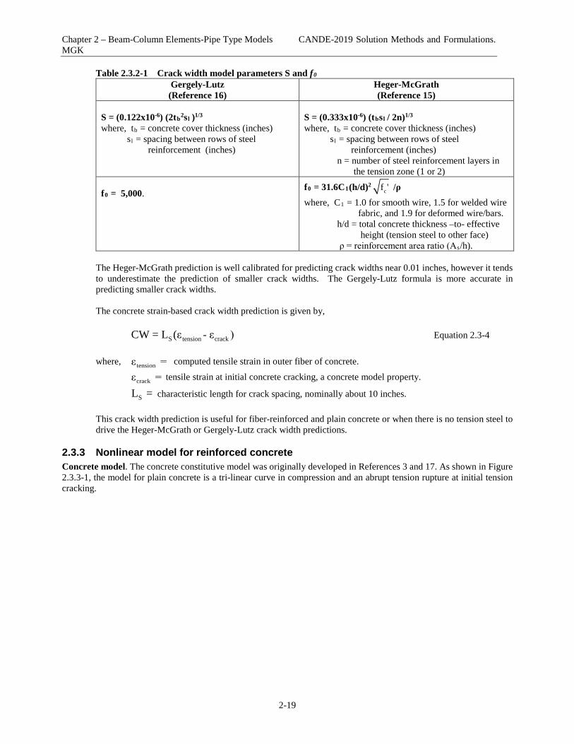
Chapter 2 – Beam-Column Elements-Pipe Type Models CANDE-2019 Solution Methods and Formulations. MGK
2-19
Table 2.3.2-1 Crack width model parameters S and f0 Gergely-Lutz (Reference 16)
Heger-McGrath (Reference 15)
S = (0.122x10⁻⁶) (2tb2sl )1/3
where, tb = concrete cover thickness (inches) sl = spacing between rows of steel reinforcement (inches)
S = (0.333x10⁻⁶) (tbsl / 2n)1/3 where, tb = concrete cover thickness (inches) sl = spacing between rows of steel reinforcement (inches) n = number of steel reinforcement layers in the tension zone (1 or 2)
f0 = 5,000.
f0 = 31.6C1(h/d)2cf ' /ρ
where, C1 = 1.0 for smooth wire, 1.5 for welded wire fabric, and 1.9 for deformed wire/bars. h/d = total concrete thickness –to- effective height (tension steel to other face) ρ = reinforcement area ratio (As/h).
The Heger-McGrath prediction is well calibrated for predicting crack widths near 0.01 inches, however it tends to underestimate the prediction of smaller crack widths. The Gergely-Lutz formula is more accurate in predicting smaller crack widths. The concrete strain-based crack width prediction is given by,
S tension crackCW = L (ε - ε ) Equation 2.3-4
where, tensionε = computed tensile strain in outer fiber of concrete.
crackε = tensile strain at initial concrete cracking, a concrete model property.
SL = characteristic length for crack spacing, nominally about 10 inches. This crack width prediction is useful for fiber-reinforced and plain concrete or when there is no tension steel to drive the Heger-McGrath or Gergely-Lutz crack width predictions.
2.3.3 Nonlinear model for reinforced concrete Concrete model. The concrete constitutive model was originally developed in References 3 and 17. As shown in Figure 2.3.3-1, the model for plain concrete is a tri-linear curve in compression and an abrupt tension rupture at initial tension cracking.

Chapter 2 – Beam-Column Elements-Pipe Type Models CANDE-2019 Solution Methods and Formulations. MGK
2-20
Figure 2.3.3-1 Concrete stress-strain model and parameters.
Primary model input parameters are defined below along with typical values shown in parenthesis ε t = concrete strain at initial tensile cracking (0.0001 in/in) ε y = concrete strain at initial elastic limit in compression (0.0006 in/in) ε c = concrete strain at onset of unconfined compressive strength (0.002 in/in) fc’ = unconfined compressive strength of concrete (4,000 psi)
E1 = Young's modulus of concrete in linear zone (3,800,000 psi) Using the above input variables, three additional parameters are derived as follows:
E2 = (fc' - E1 ε y ) / ( ε c’ - ε y ) = Young's modulus in compression yielding zone
f y c = E1 ε y = compressive stress at initial yielding (2,000 psi) f t = E1 ε t = tensile strength at initial cracking and rupture (380 psi) The following material constants are used for plane strain conditions:
21e cE = E /(1-ν ) = effective plane strain modulus of concrete in elastic zone
cν = Poisson ratio for concrete

Chapter 2 – Beam-Column Elements-Pipe Type Models CANDE-2019 Solution Methods and Formulations. MGK
2-21
r = E2/E1 = ratio of compression yielding modulus to initial modulus r eE = effective plane strain modulus for compression yielding zone. The above model has the following behavior characteristics. In tension, the concrete is linear until the initial tensile strain exceeds the cracking strain limit ε t. When cracking occurs, the tensile stress becomes abruptly zero (redistributed to non-cracked portions of concrete). Once a point in the cross section is cracked, the crack is assumed not to heal so that there is no future tensile strength. Thus after initial cracking, the tensile strength parameter f t is set to zero for all subsequent reloading in tension. For initial compression loading, the concrete behaves linearly until the stress level reaches the initial yield strength f y c after which plastic hardening begins to occur in the yield zone. Perfect plasticity occurs when the stress level reaches compressive strength fc’. Unloading is elastic and with permanent plastic strain, and reloading is elastic until the stress reaches its previous maximum value after which it follows the original stress-strain curve. Steel model. The assumed stress-strain behavior for reinforcing steel is shown in Figure 2.3.3-2. Figure 2.3.3-2 Stress-strain model for reinforcing steel.
E0
fy
- fy
Stress
StrainElastic unload path
Steel behavior is assumed to be elastic-perfectly plastic defined by the input variables:
E0 = Young's modulus for steel fy = steel yield strength
Behavior in compression and tension is identical so that material is elastic whenever the stress magnitude is less than the yield strength. Non-hardening plastic flow occurs when the stress attempts to exceed the yield strength. Unloading from the plastic range is elastic and results in permanent plastic strains. For the purposes of a plane-strain formulation, the steel modulus is denoted as; 2
s 0 sE = E /(1-υ ) = effective plane-strain modulus of steel
sυ = Poisson ratio for steel

Chapter 2 – Beam-Column Elements-Pipe Type Models CANDE-2019 Solution Methods and Formulations. MGK
2-22
Section geometry. Figure 2.3.3-3 shows a unit width of concrete wall with steel reinforcement located near the inner face (bottom) and the outer face (top). Figure 2.3.3-3 Section geometry of reinforced concrete wall
yi
yo
Aso
Asi
Unit length
h
Geometric measures of the reinforced concrete section are defined below: h = concrete wall thickness Asi = area of steel for inner cage per unit length of wall Aso = area of steel for outer cage per unit length of wall yi = distance to centroid of Asi from bottom face yo = distance to centroid of Aso from bottom face The uncracked, transformed, elastic section properties are computed as, e si soEA* = E (h + (n-1)(A +A )) Equation 2.3.3-1
2i si o soy* = ( h /2 + (n-1)(y A + y A ))/A* Equation 2.3.3-2
3 2 2 2e si i so oEI* = E [ h /12 + h(h/2-y*) + (n-1)(A (y -y*) +A (y -y*) )] Equation 2.3.3-3

Chapter 2 – Beam-Column Elements-Pipe Type Models CANDE-2019 Solution Methods and Formulations. MGK
2-23
where, n = Es/Ee = ratio of steel modulus to concrete modulus (transform method). The uncracked, transformed elastic section properties are used for the first iteration of the first load step to obtain a trial solution. If the loading does not cause cracking, concrete yielding or steel yielding, then the section properties as currently computed are correct, and the next load step is considered. More generally however, nonlinear responses are observed and iteration within the load step is required to obtain the solution as described next. Nonlinear Strategy. We assume we have a converged solution at load step i and we seek an incremental solution for load step i +1. Using the values of EA*, y* and EI* from the previous load step, a trial solution is obtained for the first iteration thereby providing new estimates of the strain distribution at each reinforced concrete cross-section. To compute the next estimate for EA*, y* and EI*, numerical integration is used over the concrete wall section to cope with nonlinear chord modulus as illustrated in the figure below. Figure 2.3.3-4 Strain profile from step i to i+1 and 11-point Simpson integration
Concrete chord modulus. The effective chord modulus, E’, from the known stress-strain state (σ i, ε i) to the estimated stress-strain state (σ i+1 , ε i+1) is computed at each integration point using the concrete stress-strain curve as indicated in Figure 2.3.3-5 and quantified in Table 2.3.3-1.

Chapter 2 – Beam-Column Elements-Pipe Type Models CANDE-2019 Solution Methods and Formulations. MGK
2-24
Figure 2.3.3-5 Illustration of concrete chord moduli from σ i, ε i to σ i+1 , ε i+1
The above figure implies the chord modulus, E’, connects the known starting point (σ i ε i,) to the estimated end point (σ i+1, ε i+1 ) where ε i+1 is obtained from the trial solution and σ i+1 is the corresponding stress determined from the stress-strain relationship as quantified in the table below. Table 2.3.3-1. Concrete chord modulus and modulus ratio for specified starting and ending zones.
Starting Zone ε i
Ending Zone ε i+1
Corresponding Stress σ i+1
Chord modulus E’
Modulus ratio F’(y) = E’/ Ee
elastic elastic σ i + EeΔε Ee 1.0 elastic yield σ i + rEe(ε i+1 - εy) rEe(ε i+1 - εy)/ Δε < 1.0 elastic plastic fc’ (fc’ - σ i)/ Δε < 1.0 yield yield σ i + rEeΔε rEe r yield plastic fc’ (fc’ - σ i)/ Δε < 1.0
plastic plastic fc’ 0.0 0.0 any compress zone unloading σ i + EeΔε Ee 1.0
elastic rupture 0.0 - σ i/ Δε < 1.0 rupture rupture 0.0 0.0 0.0
In the above table, the concrete-modulus ratio is defined as the chord modulus divided by the initial elastic modulus, F’(y) = E’/ Ee. Thus, F’ varies through the cross-section in the range, 0 ≤ F’(y) ≤ 1.

Chapter 2 – Beam-Column Elements-Pipe Type Models CANDE-2019 Solution Methods and Formulations. MGK
2-25
Elastic unloading occurs from any compression zone whenever │ε i+1│< │ε i│ with the provision that neither strain is in the rupture zone. For the case when the starting strain is tensile but not yet at initial crack strength, 0 < ε i < ε t, and the ending strain is in the rupture zone causing initial concrete cracking, we set E’ = 0 (instead of a negative softening modulus) and the pre-existing tensile stress is distributed to the uncracked portion of the cross section by adjusting the thrust and moment increment to compensate for the loss of stress at the cracked location. Once a point in the cross section is cracked the tensile strength is set to zero for all future loading conditions implying the crack does not heal. Crack depth is directly predicted from the concrete model. The above algorithm requires maintaining data records at each integration point to keep track of the cracking history as well as the maximum compressive stress encountered during the loading schedule to properly simulate unloading and reloading. Steel chord modulus. Reinforcing steel is lumped at the inner and outer cage locations, measured by yi and yo. The chord modulus for steel at either location is easily deduced from the elastic-plastic relationship as shown in the following table. Table 2.3.3-2. Steel chord modulus and modulus ratio for specified starting and ending zones.
Starting Zone ε i
Ending Zone ε i+1
Corresponding Stress σ i+1
Chord modulus Es’
Modulus ratio W’ = Es’/ Es
elastic elastic σ i + EsΔε Es 1.0 elastic plastic fy (fy - σ i)/ Δε < 1.0 plastic plastic fy 0.0 0.0
unloading elastic σ i + EsΔε Ee 1.0 In the above table, the steel-modulus ratio is defined as the chord modulus divided by the initial elastic steel modulus, W’ = Es’/ Es, where the ratio is in the range, 0 ≤ W’ ≤ 1. To summarize, the relationships for chord moduli of concrete and steel are listed below:
eE (y) = E F (y)′ ′ = concrete chord modulus at location y in cross section Equation 2.3.3-4
si s iE = E W′ ′ = steel chord modulus at inner cage location, yi. Equation 2.3.3-5
so s oE = E W′ ′ = steel chord modulus at outer cage location, yo. Equation 2.3.3-6 Re-expressing the steel chord moduli with concrete-transform parameters, we have
si i e iE = n E W′ ′ Equation 2.3.3-7
so o e oE = n E W′ ′ Equation 2.3.3-8
where, i o s en , n = E /E -1, if concrete is not cracked around the steel
i o s en , n = E /E , if concrete is cracked around the steel The transform method expresses the elastic steel modulus as a multiple “n” of the concrete elastic modulus with the understanding that the uncracked concrete area needs to be reduced by the steel area. On the other hand, if the concrete is already cracked then further reduction of concrete area by the steel area is not required. Key section properties. The equations for the key section properties are expressed in transformed parameters as:

Chapter 2 – Beam-Column Elements-Pipe Type Models CANDE-2019 Solution Methods and Formulations. MGK
2-26
h
e i i si o o so0
EA* = E ( F (y)dy + n W A + n W A )′∫ Equation 2.3.3-9
h
i i si i o o so o0
y* = ( F (y)ydy + n W A y + n W A y )/A*′∫ Equation 2.3.3-10
h2 2 2
e i i si o o so 00
EI* = E ( F (y)(y-y*) dy + n W A (y -y*) + n W A (y *) )i y′ −∫ Equation 2.3.3-11
The integrals over the concrete wall thickness is achieved with 11-point Simpson integration to evaluate the following three sums where F’(yi) is the concrete modulus ratio at integration point i.
h
1 1 2 3 110
S = F (y)dy = (h/30)[F (y )+4F (y )+2F (y )+...+F (y )]′ ′ ′ ′ ′∫ Equation 2.3.3-12
h
2 1 1 2 2 3 3 11 110
S = F (y)ydy = (h/30)[F (y )y +4F (y )y +2F (y )y +...+F (y )y ]′ ′ ′ ′ ′∫ Equation 2.3.3-13
h2 2 2 2 2
3 1 1 2 2 3 3 11 110
S = F (y)y dy = (h/30)[F (y )y +4F (y )y +2F (y )y +...+F (y )y ]′ ′ ′ ′ ′∫ Equation 2.3.3-14
Using the above integration results, the final results for the key section properties are expressed as,
e 1 i i si o o soEA* = E (S + n W A + n W A ) Equation 2.3.3-15
2 i i si i o o so oy* = (S + n W A y + n W A y )/A* Equation 2.3.3-16
2 2 2e 1 2 3 i i si i o o so 0EI* = E (y* S -2y*S +S + n W A (y -y*) + n W A (y -y*) ) Equation 2.3.3-17
Iterations with in the load step continue until successive calculations for EA*, y* and EI* are within 1% relative error for all cross section..

Chapter 2 – Beam-Column Elements-Pipe Type Models CANDE-2019 Solution Methods and Formulations. MGK
2-27
2.4 Thermoplastic Pipe
2.4.1 Overview of thermoplastic pipe type Thermoplastic materials include high-density polyethylene (HDPE), polyvinyl chloride (PVC) and polypropylene (PP). CANDE-2019 provides three options to characterize the wall sections for thermoplastic pipe: smooth, general or profile. Smooth refers to a uniform wall (gun barrel) whose cross-section properties are completely defined by the wall thickness. General refers to an arbitrary properties described generically by the wall’s area and moment of inertia per unit length. Profile refers to the majority of manufactured plastic pipe whose wall section properties are characterized by the geometry of profile elements including web, valley, crest, liner, and link elements. Material properties are assumed linear elastic with default values provided for high-density polyethylene, polyvinyl chloride and polypropylene for both short-term and long-term loading conditions. Short-term properties are generally used when vehicular loading is dominant and long-term properties are used when earth loading is dominant. A nonlinear local buckling algorithm is provided for the profile option wherein the profile’s section properties are reduced in proportion to the amount of compressive strain computed in the sub elements due to local buckling.
2.4.2 Design criteria for thermoplastic pipe Design criteria for thermoplastic pipes include strength limits for thrust stress against material failure in hoop compression and global buckling. Another strength state is a limit on the maximum outer fiber combined strain (hoop plus bending strain). Performance limit states include allowable vertical deflection and maximum allowable tensile strain, dependent on type of plastic. The design criteria are summarized in the following table. Table 2.4.2-1 Thermoplastic Design Criteria.
Design Criterion (Strength limits)
Demand Capacity
(1) Thrust stress (psi) max maxσ = N /A uf = ultimatestrength
(2) Global Buckling (psi) max maxσ = N /A bf = buckling capacity
(3) Combined strain (in/in) maxε = bending + thrust ultε = ultimatestrain
(Performance Limits) (at Service Load)
(4) Allowable tensile strain -maxtε =max tensilestrain t-allowε = allowable tensilestrain
(5) Allowable deflection *(%) maxΔ = computed deflect % Allowable = 5%
(recommended) The above design criteria are equally applicable to working stress or LRFD design methodologies. For the working stress approach, the demand and the capacity quantities are unfactored, and the design evaluation is given by safety factors defined as capacity divided by demand. Typically safety factors on the order of 2.0 are desirable for strength-related criteria. For the LRFD approach the demand and the capacity quantities are factored (see Chapter 6), and the design evaluation is given by ratios of factored demand-to-factored capacity. Ratios less than or equal to 1.0 are acceptably safe. Further discussion on the design criteria is provided below.
1. Thrust stress. Thrust-stress demand is computed by the dividing the maximum thrust force in the culvert by the cross-sectional area. The ultimate strength for thrust stress is dependent on the type plastic and the load duration. Nominal values, taken from the ASSHTO LRFD specifications and elsewhere, are shown in the table below.

Chapter 2 – Beam-Column Elements-Pipe Type Models CANDE-2019 Solution Methods and Formulations. MGK
2-28
Table 2.4.2-2 Recommended plastic properties for short and long-term loading Type of plastic
Effective Young’s Modulus (PE)
Ultimate strength (PU)
Short-term (ksi)
Long-term (ksi)
Short-term (ksi)
Long-term (ksi)
HDPE –
110.0
22.0
3.00
0.90
PVC –
400.0
140.0
6.00
2.60
PP –
135.0
27.0
3.10
1.00
2. Global buckling. The thrust stress level that causes global buckling may be conservatively approximated from the simplified AASHTO LRFD equations 12.7.2.4-1-2. A more accurate alternative is to utilize the new large deformation formulation with buckling capacity prediction available in CANDE-2019 (see Chapter 5).
3. Combined strain. Combined strain means the maximum outer-fiber strain from thrust and bending and the
demand is the largest combined strain anywhere in the culvert. The combined strain limit value (or capacity) as recommended by AASHTO LRFD specifications is equal to 1.5 times the long-term strength divided by the long-term modulus. Accordingly, HDPE = 0.06 in/in, PVC = 0.028 in/in. and PP = 0.045 in/in.
4. Allowable tensile strain. This criterion is intended to preclude cracking and crazing under service load due the
maximum outer-fiber tensile strain. The allowable tensile strain as recommended by AASHTO LRFD specifications is 0.05 in/in for HDPE and 0.035 or 0.05 in/in for PVC depending on cell class.
5. Allowable deflection. Computed deflection is the relative vertical movement between the top and bottom of the
culvert structure, and the percent deflection is relative the vertical distance. The service load value for allowable deflection is generally taken as 5% of the diameter for all plastic pipes; however, the deflection limit is not directly specified in the AASHTO LRFD design specifications.
Local Buckling. Local buckling is not a direct design criterion for plastic pipe, but it does influence the demands and capacities of the design criteria listed above. Similar to corrugated metal pipe wherein some amount of outer fiber yielding is permitted, some amount of local buckling is permitted in plastic profile pipe. The nonlinear model to account for local buckling in profile plastic pipe is presented next.
2.4.3 Nonlinear model for local buckling in profile plastic pipe Although the stress-strain models for all thermoplastic pipe materials are assumed linear and characterized by the elastic moduli in the above table, local buckling is a nonlinear phenomenon. Local buckling is caused by compressive strains that induce the elements of profile wall pipe to deform out-of-plane in a wrinkled pattern. Section 12.12.3.5.3 of AASHTO LRFD specifications provides a methodology to simulate the effect of local buckling by reducing the effective area of the profile elements dependent upon the average level of compressive strain in each element. This AASHTO methodology is incorporated into CANDE-2019 as described below. The geometry of the profile wall is defined with two web elements and up to four horizontal elements (valley, liner, crest and link) as shown in the figure below. Older versions of CANDE assumed the profile configuration was constant for the entire pipe group; however, the newer versions permit varying the profile geometric properties within the pipe group.

Chapter 2 – Beam-Column Elements-Pipe Type Models CANDE-2019 Solution Methods and Formulations. MGK
2-29
Figure 2.4.3-1 Profile wall geometry and sub elements
Link (4)Link (4) Crest (3)
Valley (1) Valley (1)Liner (2)
WebWeb
Period
Height
The web element lengths, which form a mirror symmetric pair within each period, are defined to span the distance between the valley and crest element so that the web elements offer support to the ends of the crest and valley elements. Hence, the defined length of the crest element is the unsupported span between the web supports plus the length of the web supports, taken as twice the web thickness. Similarly, the defined length of the valley element is twice the web thickness plus the unsupported valley span between the web supports. The defined length of the liner element is the horizontal distance between two valley elements so that the liner’s defined length and unsupported length are identical. Similarly, the defined length of the link element is the horizontal distance between two crest elements so that the crest’s defined length and unsupported length are identical. Given the defined lengths and thicknesses of all elements, the angle of the web elements, and the overall height of the profile wall, it is a straightforward matter to calculate the initial section properties of the profile wall. The area per unit length, A*, is equal to the sum of all element areas (lengths multiplied by thickness) divided by the period length. The wall centroid, y*, is the first area moment taken about the bottom fiber divided by the area. And finally, the moment inertia per unit length , I*, is the second area moment taken about y* divided by the period length. Thus in the absence of local buckling, the beam-column section properties are initially known for the first iteration of the first load step to provide the first trial solution. The AASHTO LRFD methodology, which accounts for local buckling by reducing the effective length of the elements due to compressive strain, is achieved by using the following two equations.
λ = (w/t) (ε/k) > 0.673 Equation 2.4-1 where, λ = measure of propensity to buckle, called slenderness ratio w = unsupported length of element t = thickness of element ε = average compressive strain in element k = edge support coefficient (typically taken as 4.0 for fix-ended elements)
ρ = (1/λ) (1 - 0.22/λ) < 1.0 Equation 2.4-2 where, ρ = reduction factor applied to w ρw = remaining unsupported length of element Each profile element (web, valley, liner, crest and link ) is evaluated with above equations. Equation 2.4-1 is evaluated to compute λ using the predicted compressive strain at each element’s centroid as determined from the trial solution. If λ

Chapter 2 – Beam-Column Elements-Pipe Type Models CANDE-2019 Solution Methods and Formulations. MGK
2-30
< 0.673, then the compressive strain is not large enough to trigger local buckling for the element under consideration so that ρ remains = 1. Otherwise if λ > 0.673, we evaluate Equation 2.4.2 producing a value for ρ less than 1.0 wherein ρ is the fraction of the element’s unsupported length that remains effective in the cross section. Note that the total effective length for the crest and valley elements also includes the web support thicknesses. The element length measures are clarified in the table below: Table 2.4.3-1 Local buckling profile dimensions
Element length measures
Symbol Derivation Description
Defined length L Defined by user (input)
The actual length of the element
Unsupported length w w = L, (for web, liner and link) w = L – 2tweb, (for crest & valley)
The free distance between supports where buckling can occur
Effective length
Leff Leff = ρL, (for web, liner and link) Leff = ρw + 2tweb, (for crest & valley)
The effective remaining length of element after local buckling
Since the central portion of each element is the most prone to local buckling damage, we assume the original element length has effective gap length equal to L - Leff located in the central portion of the element. This assumption is needed to compute the effective moment of inertia. Once the effective lengths of the elements have been determined and the location of the gaps understood, it is, once again, a straightforward matter to calculate the new section properties for the next trial solution as; A* = Sum of all effective element areas (effective lengths times thicknesses) y* = Centroid of A* measured from bottom fiber I* = Sum of all effective element moment of inertias about y* The above process dovetails with the general nonlinear solution strategy described in Section 2.19 by forming EA* and EI* where E is the appropriate linear elastic modulus (Table 2.4.2-2). When two successive trial solutions produce the same compressive stain values within a 0.1% tolerance level for all elements at all nodes, the load step is said to converge and we proceed to the next load step.

Chapter 2 – Beam-Column Elements-Pipe Type Models CANDE-2019 Solution Methods and Formulations. MGK
2-31
2.5 Basic Pipe Type The so-called basic pipe-type is not associated with any particular pipe material. Therefore, it is restricted to linear material behavior, and it is not associated with any design criteria for evaluating its safety or performance. The material model is defined by an elastic Young’s modulus and Poisson’s ratio, and the cross-sectional properties are defined an area and moment of inertia. If desired, each element in the basic pipe-type group may be assigned different elastic and cross-sectional properties, and the element group has the option to include large deformation theory and buckling capacity predictions. In addition to academic studies, the basic pipe-type groups are useful for modeling struts and braces and discrete reinforcement in the soil mass. Lastly, if it is desired to use only continuum elements without beam-column elements in particular problem in the CANDE-2019 program, the basic pipe type is declared in the input with zero elements assigned to the group.
2.6 Conrib Pipe Type The figure below represents one example of the potential use of the CONRIB pipe type for modeling precast arch units with ribbed stiffeners along the crown as well as T-shaped stiffeners cast into the supporting pedestal walls. These ribbed and/or T-shaped stiffeners cannot be modeled with the standard CONCRETE pipe type. Another special feature of the CONRIB pipe type is an advanced concrete constitutive model that is capable of simulating fiber reinforced concrete in addition to standard concrete with traditional steel reinforcement.
This section provides a detailed formulation of the CONRIB pipe type using the same presentation outline that is used for all other pipe-types in this chapter. The reader is referred to the beginning of Chapter 2 to review the general background development for the beam-column element, which is applicable to all pipe types. Although some of the aspects of the CONRIB model are similar or nearly identical to the CONCRETE pipe type, the following development is self-contained without referring the reader the CONCRETE model write up. The ultimate goal is to derive the incremental stiffness matrices and nonlinear solution strategy even though some of the derivation is repetitive of the CONCRETE write-up.
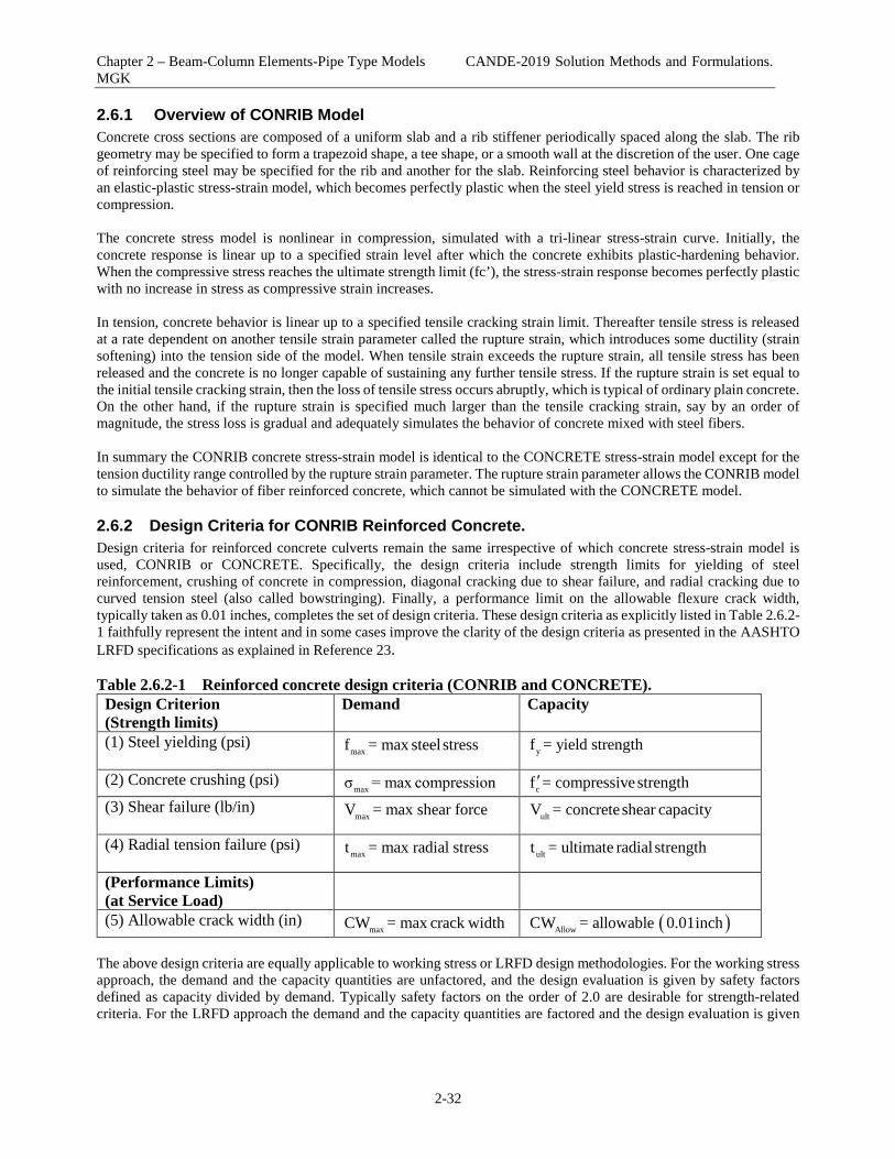
Chapter 2 – Beam-Column Elements-Pipe Type Models CANDE-2019 Solution Methods and Formulations. MGK
2-32
2.6.1 Overview of CONRIB Model Concrete cross sections are composed of a uniform slab and a rib stiffener periodically spaced along the slab. The rib geometry may be specified to form a trapezoid shape, a tee shape, or a smooth wall at the discretion of the user. One cage of reinforcing steel may be specified for the rib and another for the slab. Reinforcing steel behavior is characterized by an elastic-plastic stress-strain model, which becomes perfectly plastic when the steel yield stress is reached in tension or compression. The concrete stress model is nonlinear in compression, simulated with a tri-linear stress-strain curve. Initially, the concrete response is linear up to a specified strain level after which the concrete exhibits plastic-hardening behavior. When the compressive stress reaches the ultimate strength limit (fc’), the stress-strain response becomes perfectly plastic with no increase in stress as compressive strain increases. In tension, concrete behavior is linear up to a specified tensile cracking strain limit. Thereafter tensile stress is released at a rate dependent on another tensile strain parameter called the rupture strain, which introduces some ductility (strain softening) into the tension side of the model. When tensile strain exceeds the rupture strain, all tensile stress has been released and the concrete is no longer capable of sustaining any further tensile stress. If the rupture strain is set equal to the initial tensile cracking strain, then the loss of tensile stress occurs abruptly, which is typical of ordinary plain concrete. On the other hand, if the rupture strain is specified much larger than the tensile cracking strain, say by an order of magnitude, the stress loss is gradual and adequately simulates the behavior of concrete mixed with steel fibers. In summary the CONRIB concrete stress-strain model is identical to the CONCRETE stress-strain model except for the tension ductility range controlled by the rupture strain parameter. The rupture strain parameter allows the CONRIB model to simulate the behavior of fiber reinforced concrete, which cannot be simulated with the CONCRETE model.
2.6.2 Design Criteria for CONRIB Reinforced Concrete. Design criteria for reinforced concrete culverts remain the same irrespective of which concrete stress-strain model is used, CONRIB or CONCRETE. Specifically, the design criteria include strength limits for yielding of steel reinforcement, crushing of concrete in compression, diagonal cracking due to shear failure, and radial cracking due to curved tension steel (also called bowstringing). Finally, a performance limit on the allowable flexure crack width, typically taken as 0.01 inches, completes the set of design criteria. These design criteria as explicitly listed in Table 2.6.2-1 faithfully represent the intent and in some cases improve the clarity of the design criteria as presented in the AASHTO LRFD specifications as explained in Reference 23. Table 2.6.2-1 Reinforced concrete design criteria (CONRIB and CONCRETE).
Design Criterion (Strength limits)
Demand Capacity
(1) Steel yielding (psi)
maxf = max steel stress yf = yield strength
(2) Concrete crushing (psi) maxσ = max compression cf = compressivestrength′
(3) Shear failure (lb/in)
maxV = max shear force ultV = concrete shear capacity
(4) Radial tension failure (psi)
maxt = max radial stress ultt = ultimate radial strength
(Performance Limits) (at Service Load)
(5) Allowable crack width (in) maxCW = max crack width ( )AllowCW = allowable 0.01inch
The above design criteria are equally applicable to working stress or LRFD design methodologies. For the working stress approach, the demand and the capacity quantities are unfactored, and the design evaluation is given by safety factors defined as capacity divided by demand. Typically safety factors on the order of 2.0 are desirable for strength-related criteria. For the LRFD approach the demand and the capacity quantities are factored and the design evaluation is given

Chapter 2 – Beam-Column Elements-Pipe Type Models CANDE-2019 Solution Methods and Formulations. MGK
2-33
by ratios of demand-to-capacity. Demand-to-capacity ratios less than or equal to 1.0 are acceptably safe. Further discussion on the design criteria is provided below.
6. Steel yielding. The maximum steel-stress demand is computed directly from the nonlinear reinforced concrete model. On the capacity side, the steel yield strength is an input or default value, nominally 60,000 psi for deformed bars and 65,000 psi for smooth wire fabric.
7. Concrete crushing. On the demand side, the maximum outer-fiber concrete compressive stress is determined
directly from the reinforced concrete model as a result of thrust and compression bending. The ultimate compressive strength or capacity is an input or default value typically in the range of 4000 to 6000 psi.
8. Shear failure. The maximum shear-force demand is computed directly from the beam-column internal forces.
Shear-force capacity is the shear force causing diagonal tension failure at a given cross-section. AASHTO LRFD specifications prescribe three different shear-force capacities depending on structural shape and burial depth.
• For concrete pipes and arches, the shear capacity is specified by Vmax = Equations 12.10.4.2.5,
which yield variable values for shear capacity dependent on the values for moment, thrust and shear around the culvert wall.
• For boxes and 3-sided structures with 2 or more feet of soil cover, the shear capacity is specified
by Vmax = Equations 5.14.5.3-1 wherein the value is dependent on moment and shear (not thrust).
• For boxes and 3-sided structures with less than 2 feet of soil cover, the shear capacity is specified by equations in Section 5.8.3.3 that, in some cases, depend on the nature of the traverse reinforcement (stirrups).
Clearly there is a need to unify the AASHTO shear-capacity equations because rational mechanics indicates that shear capacity should be a function of the cross-section properties and state of loading, not on the culvert shape or depth of burial. CANDE allows the user to select among the three choices for shear-force capacity, however, Equation 12.10.4.2.5 is considered the best predictor of shear-force capacity because of the large experimental database (Reference 14). CANDE also provides the option to choose the traditional shear-strength method where shear-strength = β cf ′
, where β is a specified factor, typically = 2.0.
9. Radial tension failure. On the demand side, the concrete radial tensile stress is caused by tensile forces in curved inner cage reinforcement steel as it tends to straighten out and exerts radial tensile stresses on the interior concrete cover thickness. The phenomenon is sometimes called bow stringing. CANDE predicts the radial tensile stress by dividing the interior cage steel force (maximum tensile force per unit length) by the radius of curvature of the steel cage, i.e., letting As = steel area per unit length., we have;
max s maxt = A f /Radius Equation 2.6-1
The ultimate radial stress is related to the tension strength of concrete and the structure span. The radial tensile strength capacity is adapted from AASHTO LRFD Equation 12.10.4.2.4c-1. and restated in psi units as:
ult rtct = 37.92 f /1000 F ′ Equation 2.6-2
where Frt is a scale factor dependent on structure span, specified in the contents of AASHTO LRFD Equation 12.10.4.2.4c-1.

Chapter 2 – Beam-Column Elements-Pipe Type Models CANDE-2019 Solution Methods and Formulations. MGK
2-34
10. Allowable crack width. The allowable crack width at service loading is generally taken as 0.01 inches in accordance with AASHTO LRFD specification 12.10.3. CANDE offers three empirical formulas to predict crack width; the traditional Gergely-Lutz formula (Reference 16), the recently developed Heger-McGrath formula (modified form from Reference 15), and a simple concrete strain-based formula proposed by Katona.
The Gergely-Lutz and Heger-McGrath equations are similar in form and are driven by the computed tension steel stress when it exceeds f0 , the threshold stress for initial cracking. Their crack width predictions are concisely stated in the equation below,
s 0CW = S(f - f ) > 0 Equation 2.6-3 where, CW = the crack width in inches,
fs = computed tension steel stress in psi, S and f0 = model parameters specified in the table below.
Table 2.6.2-2 Crack width model parameters S and f0
Gergely-Lutz
Heger-McGrath
S = (0.122x10⁻⁶) (2tb
2sl )1/3
where, tb = concrete cover thickness (inches) sl = spacing between rows of steel (inches).
S = (0.333x10⁻⁶) (tbsl / 2n)1/3 where, tb = concrete cover thickness (inches) sl = spacing between rows of steel (inches) n = number of steel layers in the tension zone (1 or 2)
f0 = 5,000.
f0 = 31.6C1(h/d)2cf ' /ρ
where, C1 = 1.0 for smooth wire, 1.5 for welded wire fabric, and 1.9 for deformed wire/bars. h/d = total concrete thickness –to- effective height (tension steel to other face) ρ = reinforcement area ratio (As/h).
The Heger-McGrath prediction is well calibrated for predicting crack widths near 0.01 inches, however it tends to
underestimate the prediction of smaller crack widths. The Gergely-Lutz formula is more accurate in predicting smaller crack widths. The concrete strain-based crack width prediction is given by,
S tension crackCW = L (ε - ε ) Equation 2.6-4
where, tensionε = computed tensile strain in outer fiber of concrete.
crackε = tensile strain at initial concrete cracking, a concrete model property.
SL = characteristic length for crack spacing, nominally about 10 inches. This crack width prediction is useful for fiber-reinforced and plain concrete or when there is no tension steel to drive the Heger-McGrath or Gergely-Lutz crack width predictions.

Chapter 2 – Beam-Column Elements-Pipe Type Models CANDE-2019 Solution Methods and Formulations. MGK
2-35
2.6.3 CONRIB concrete model. As shown in Figure 2.6.3-1, the CONRIB concrete model is a tri-linear curve in compression exactly the same as the CONCRETE model for plain concrete. In the tension zone, however, the CONRIB model has the capability of simulating varying amounts of ductility depending on the values assigned to the initial cracking strain and rupture strain parameters. If the rupture strain parameter is set equal to the initial tension cracking strain, then there is no ductility and the CONRIB model behaves like plain concrete with an abrupt loss of all tensile stress once the initial cracking strain is reached. On the other hand, if the rupture strain parameter is assigned a value larger than the initial cracking strain, the model exhibits a ductile behavior with a gradual loss of tensile stress such that the larger the value of the rupture strain the greater the amount of ductility. Figure 2.6.3-1 Concrete stress-strain model and parameters.
Primary model input parameters are defined below along with typical values shown in parenthesis ε c = concrete strain at onset of unconfined compressive strength (0.002 in/in)
ε y = concrete strain at initial elastic limit in compression (0.0006 in/in) ε t = concrete strain at initial tensile cracking (0.0001 in/in) є r = concrete strain at tensile rupture (0.0001 to .01 in/in)
fc’ = unconfined compressive strength of concrete (4,000 psi) E1 = Young's modulus of concrete in linear zone (3,800,000 psi)
Using the above input variables, four additional parameters are derived as follows:

Chapter 2 – Beam-Column Elements-Pipe Type Models CANDE-2019 Solution Methods and Formulations. MGK
2-36
E2 = (fc' - E1 ε y ) / ( ε c’ - ε y ) = Young's modulus in compression yielding zone f y c = E1 ε y = compressive stress at initial yielding (2,000 psi)
f t = E1 ε t = tensile strength at initial cracking and rupture (380 psi) E3 = - f t /(є r - ε t) = tension-softening modulus (negative) The following material constants are used for plane strain conditions: cν = Poisson ratio for concrete
21e cE = E /(1-ν ) = effective plane strain modulus of concrete in elastic zone
2c 2E = E /(1-ν ) = effective plane strain modulus in concrete yield zone
2s 3E = E /(1-ν ) = effective plane strain modulus in ductile softening zone
The above model has the following behavior characteristics. For initial compression loading, the concrete behaves linearly until the stress level reaches the initial yield strength f y c after which plastic hardening begins to occur in the yield zone. Perfect plasticity occurs when the stress level reaches compressive strength fc’. Unloading is elastic and with permanent plastic strain, and reloading is elastic until the stress reaches its previous maximum value after which it follows the original stress-strain curve. In tension, the concrete is linear until the initial tensile strain exceeds the cracking strain limit ε t. After tensile cracking occurs, the tensile stress is reduced in the softening range at a rate depending on the softening modulus (negative value). Finally, when the strain exceeds the rupture strain all stress is released inferring that all fibers bridging the crack are broken or pulled out. When this occurs, the crack is assumed not to heal so that there is no future tensile strength at this point. However if the strain is reversed prior to reaching the rupture strain, then the remaining tension stress is preserved and the ductile zone is characterized with a reduced tensile strength for future tensile loading.
2.6.4 Reinforcement steel model The assumed stress-strain behavior for reinforcing steel is shown in Figure 2.6.4-1. Figure 2.6.4-1 Stress-strain model for reinforcing steel.
Steel behavior is assumed to be elastic-perfectly plastic defined by the input variables:
E0 = Young's modulus for steel fy = steel yield strength

Chapter 2 – Beam-Column Elements-Pipe Type Models CANDE-2019 Solution Methods and Formulations. MGK
2-37
Behavior in compression and tension is identical so that material is elastic whenever the stress magnitude is less than the yield strength. Non-hardening plastic flow occurs when the stress attempts to exceed the yield strength. Unloading from the plastic range is elastic and results in permanent plastic strains. For the purposes of a plane-strain formulation, the steel modulus is denoted as; 2
s t 0 s tE = E /(1-υ ) = effective plane-strain modulus of steel
s tυ = Poisson ratio for steel
2.6.5 Concrete cross-section geometry Figure 2.6.5-1 shows one period of concrete rib wall with steel reinforcement located near the inner face (bottom) and the outer face (top). Although not shown, the alternative orientation is with the rib pointing in the outward direction, which is developed in the same manner as the orientation shown below. Figure 2.6.5-1 Section geometry of reinforced concrete rib wall
Geometric measures of the general concrete rib section are defined below. (Note that a smooth wall section is obtained by setting rs = rw = rj.) rs = rib spacing on centers along culvert length rw = rib width at bottom rj = rib width at junction with slab
h = total concrete wall thickness, rib plus slab hr = concrete rib thickness hs = h – hr = concrete slab thickness

Chapter 2 – Beam-Column Elements-Pipe Type Models CANDE-2019 Solution Methods and Formulations. MGK
2-38
Steel reinforcement parameters are defined below. siA = area of steel in rib divided by actual rib width through steel centroid Aso = area of steel in slab per unit length of slab yi = ci = distance to centroid of Asi from bottom face yo = h – co = distance to centroid of Aso from bottom face Note that for ease of input, the steel area in the rib siA is defined as area per unit length of rib, not per unit length of the period. Therefore the rib area as input is corrected to the common rib spacing value for computing section properties as follows. Asi = (rc/ rs) siA Equation 2.6.5-1 where, rc = rw + (yi/h)( rj - rw) = rib width at level of steel centroid. With the above understandings, the uncracked, transformed, elastic section properties for area stiffness, neutral axis and bending stiffness are computed as follows.
e si soj w
s rs
EA* = E (h + (n-1)(A +A ))r +r
+ h2r
Equation 2.6.5-2
i si o soj w 2
s s rs
y* = (h h /2) + + (n-1)(y A + y A ))/A*r +r
(h+ h3r
Equation 2.6.5-3
3e
j w j w3 2 2 2 3 2r r r r r
s s
EI* = E [ (h /3 - y*( h + y* (h-h3r +r 2r +r
-h ) -h ) ) + h - y* h12r 3r
2 2si i so o
j w2r
s
(n-1)(A (y -y*) +A (y -y*) )]r +r
+ y* h + 2r
Equation 2.6.5-4
where, n = Est/Ee = ratio of steel modulus to concrete modulus (transform method). The uncracked, transformed elastic section properties are used for the first iteration of the first load step to obtain a trial solution. If the loading does not cause cracking, concrete yielding or steel yielding, then the section properties as currently computed are correct, and the next load step is considered. More generally however, nonlinear responses are observed and iteration within the load step is required to obtain the solution as described next.
2.6.6 Nonlinear solution strategy. We assume we have a converged solution at load step i and we seek an incremental solution for load step i +1. Using the values of EA*, y* and EI* from the previous load step, a trial solution is obtained for the first iteration thereby providing new estimates of the strain distribution at each reinforced concrete cross-section. To compute the next estimate for EA*, y* and EI*, numerical integration is used over the concrete wall section to cope with nonlinear chord modulus as illustrated in the figures below.

Chapter 2 – Beam-Column Elements-Pipe Type Models CANDE-2019 Solution Methods and Formulations. MGK
2-39
Figure 2.6.6-1 Strain profile from step i to i+1 and 11-point Simpson integration
Concrete chord modulus. The effective chord modulus, E’, from the known stress-strain state (σ i, ε i) to the estimated stress-strain state (σ i+1 , ε i+1) is computed at each integration point using the concrete stress-strain curve previously illustrated in Figure 2.6.3-1. As discussed in the following sections, the chord modulus is determined iteratively. The Figure 2.6.6-2 illustrates various chord moduli, E’, which connects a known starting point (σ i ε i,) to the estimated end point (σ i+1, ε i+1 ). Here, ε i+1 is obtained from the trial incremental solution, ε i+1 = ε i +Δε, and σ i+1 is the corresponding stress determined from the stress-strain relationship as quantified in the Table 2.6.6-1. Figure 2.6.6-2 Illustration of concrete chord moduli in zone transitions

Chapter 2 – Beam-Column Elements-Pipe Type Models CANDE-2019 Solution Methods and Formulations. MGK
2-40
Table 2.6.6-1. Concrete chord modulus and ratio for specified starting and ending zones.
Starting Zone ε i
Ending Zone ε i+1
Corresponding Stress σ i+1
Chord modulus E'
Modulus ratio F'(y) = E'/ Ee
elastic elastic σ i + EeΔε Ee = 1.0 elastic yield fy + Ec(ε i+1 - εy) (σ i+1 - σ i )/ Δε < 1.0 elastic plastic fc' (fc' - σ i)/ Δε < 1.0 yield more yield σ i + EcΔε Ec = Ec/ Ee yield plastic fc' (fc' - σ i)/ Δε < Ec/ Ee
plastic more plastic fc' 0.0 = 0.0 compress zone unloading σ i + EeΔε Ee = 1.0
elastic soften ft + Es(ε i+1 – ε t) (σ i+1 - σ i )/ Δε < 1.0 soften more soften σ i + EsΔε Es < 0.0 soften rupture 0.0 - σ i / Δε < 0.0 rupture more rupture 0.0 0.0 = 0.0
In the above table, the concrete-modulus ratio is defined as the chord modulus divided by the initial elastic modulus, F'(y) = E'/Ee. Thus, F'(y) varies through the cross-section including negative values for integration points in the softening range. Elastic unloading occurs from any compression zone whenever │ε i+1│< │ε i│ with the provision that neither strain is in the softening or rupture zone. Once a point in the cross section begins to crack, the initial tensile strength is permanently reduced to the corresponding stress value on the softening leg of the stress-strain curve. Physically this means some tension damage has occurred changing the shape of the stress-strain path in the tension zone. When the tensile strain exceeds the rupture strain, the tension damage is complete and the stress-strain path is completely flat in tension for all future tensile loading conditions, implying the crack does not heal. The above algorithm requires maintaining data records at each integration point to keep track of the cracking history and tension damage. It is also required to maintain a data record of plastic straining in compression in order to properly simulate unloading and reloading. Steel chord modulus. Reinforcing steel is lumped at the inner and outer cage locations, measured by yi and yo. The chord modulus for steel at either location is easily deduced from the elastic-plastic relationship as shown in the following table. Table 2.6.6-2. Steel chord modulus and ratio for specified starting and ending zones.
Starting Zone ε i
Ending Zone ε i+1
Corresponding Stress σ i+1
Chord modulus Es'
Modulus ratio W' = Es'/ Est
elastic elastic σ i + EstΔε Est 1.0 elastic plastic fy (fy - σ i)/ Δε < 1.0 plastic plastic fy 0.0 0.0
unloading elastic σ i + EstΔε Est 1.0 In the above table, the steel-modulus ratio is defined as the chord modulus divided by the initial elastic steel modulus, W' = Es'/ Est, where the ratio is in the range, 0 ≤ W' ≤ 1. To summarize, the relationships for chord moduli of concrete and steel are listed below:

Chapter 2 – Beam-Column Elements-Pipe Type Models CANDE-2019 Solution Methods and Formulations. MGK
2-41
eE (y) = E F (y)′ ′ = concrete chord modulus at location y Equation 2.6.6-1
si st iE = E W′ ′ = steel chord modulus at inner cage location, yi. Equation 2.6.6-2
so st oE = E W′ ′ = steel chord modulus at outer cage location, yo. Equation 2.6.6-3 Re-expressing the steel chord moduli with concrete-transform parameters, we have
si i e iE = n E W′ ′ Equation 2.6.6-4
so o e oE = n E W′ ′ Equation 2.6.6-5
where, i o st en , n = E /E -1, if concrete is not cracked around the steel
i o st en , n = E /E , if concrete is cracked around the steel The transform method expresses the elastic steel modulus as a multiple “n” of the concrete elastic modulus with the understanding that the uncracked concrete area needs to be reduced by the steel area to avoid double counting areas. On the other hand, if the concrete is already cracked then further reduction of concrete area by the steel area is not required. Computing section properties. Section properties require area integration over the concrete cross section. To this end, the differential area is expressed as dA = b(y)dy where b(y) is the effective cross-section width per unit length as defined below.
w j w s
1.0, if y is in the slab zone b(y) = y(r + (r -r ))/r , if y is in the rib zone
h
Equation 2.6.6-6
With the above understanding, the equations for the key section properties are expressed in transformed parameters as follows.
h
e i i si o o so0
EA* = E ( F (y)b(y)dy + n W A + n W A )′∫ Equation 2.6.6-7
h
i i si i o o so o0
y* = ( F (y)yb(y)dy + n W A y + n W A y )/A*′∫ Equation 2.6.6-8
h2 2 2
e i i si i o o so 00
EI* = E ( F (y)(y-y*) b(y)dy + n W A (y -y*) + n W A (y -y*) )′∫
Equation 2.6.6-9 The integrals over the concrete wall thickness is achieved with 11-point Simpson integration to evaluate the following three sums where F'(yi) ≤ 1.0 is the concrete modulus ratio at integration point i, and b(yi) ≤ 1.0 is the effective cross-section width per unit length.
h
1 1 1 2 2 3 3 11 110
S = F (y)b(y)dy = h/30[F (y )b(y )+4F (y )b(y )+2F (y )b(y )+...+F (y )b(y )]′ ′ ′ ′ ′∫
Equation 2.6.6-10 h
2 1 1 1 2 2 2 3 3 3 11 11 110
S = F (y)yb(y)dy = h/30[F (y )y b(y )+4F (y )y b(y )+2F (y )y b(y )+...+F (y )y b(y )]′ ′ ′ ′ ′∫
Equation 2.6.6-11

Chapter 2 – Beam-Column Elements-Pipe Type Models CANDE-2019 Solution Methods and Formulations. MGK
2-42
h2 2 2 2 2
3 1 1 1 2 2 2 3 3 3 11 11 110
S = F (y)y b(y)dy = h/30[F (y )y b(y )+4F (y )y b(y )+2F (y )y b(y )+...+F (y )y b(y )]′ ′ ′ ′ ′∫
Equation 2.6.6-12 Using the above integration results, the final results for the key section properties are expressed as,
e 1 i i si o o soEA* = E (S + n W A + n W A ) Equation 2.6.6-13
2 i i si i o o so oy* = (S + n W A y + n W A y )/A* Equation 2.6.6-14
2 2 2e 1 2 3 i i si i o o so 0EI* = E (y* S -2y*S +S + n W A (y -y*) + n W A (y -y*) ) Equation 2.6.6-15
The above calculations are carried out in subroutine Conmax, which is called by subroutine Conrib. Iterations within the load step continue until successive calculations for EA*, y* and EI* are within 1% relative error for all cross sections.
2.6.7 CONRIB Model Behavior and Parameter Identification When comparing the stress-strain models of plain concrete model with the ductile CONRIB model, it may seem that the load capacities of the two models would be the same if the tensile strength and compressive strength were the same. Indeed, this observation is true for test specimens loaded in pure axial tension or pure axial compression. For these cases, the ultimate axial load is easily computed as recorded below and is independent of ductility parameters. tT = f A = ultimate tensile load Equation 2.6.7-1
cC = f A′ = ultimate compressive load Equation 2.6.7-2 where, tf = tensile strength of concrete
cf ′ = compressive strength of concrete
A = cross-sectional area of the test specimen. However for a test specimen loaded in pure bending, it is quite remarkable that the ultimate moment capacity of the ductile CONRIB model is appreciably greater than the plain concrete model depending on the value of the ductility strain ratio defined as follows. r tr = ε /ε = ductility strain ratio (r ≥ 1) Equation 2.6.7-3 where, rε = rupture strain
tε = initial cracking strain When the ratio r = 1, there is no ductility and the CONRIB model behaves like plain concrete, exhibiting an abrupt loss of the internal moment once the initial cracking moment is reached. However for r > 1, the moment capacity increases with r and exhibits gradual strength loss.
2.6.8 Derivation of moment capacity in pure bending Consider a beam specimen in pure bending with a rectangular cross-section of height h and width b as shown in Figure 2.6.8-1. Because planes remain plane in bending, the strain profile is linear through the height of the cross section for all
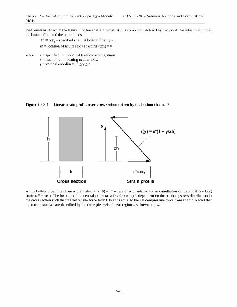
Chapter 2 – Beam-Column Elements-Pipe Type Models CANDE-2019 Solution Methods and Formulations. MGK
2-43
load levels as shown in the figure. The linear strain profile ε(y) is completely defined by two points for which we choose the bottom fiber and the neutral axis.
tε* = xε = specified strain at bottom fiber, y = 0 zh = location of neutral axis at which ε(zh) = 0
where x = specified multiplier of tensile cracking strain. z = fraction of h locating neutral axis. y = vertical coordinate, 0 ≤ y ≤ h Figure 2.6.8-1 Linear strain profile over cross section driven by the bottom strain, ε*
At the bottom fiber, the strain is prescribed as ε (0) = ε* where ε* is quantified by an x-multiplier of the initial cracking strain (ε* = xε t ). The location of the neutral axis z (as a fraction of h) is dependent on the resulting stress distribution in the cross section such that the net tensile force from 0 to zh is equal to the net compressive force from zh to h. Recall that the tensile stresses are described by the three piecewise linear regions as shown below.

Chapter 2 – Beam-Column Elements-Pipe Type Models CANDE-2019 Solution Methods and Formulations. MGK
2-44
Figure 2.6.8-2 Tension portion of CONRIB model with ductility (fiber reinforcement)
With the above understanding, the applied maximum tensile strain on the bottom fiber ε* is in one of three ranges depending on the magnitude of x.
1. ε* is in the uncracked elastic range, 0 ≤ x ≤ 1 2. ε* is in the softening range, 1 ≤ x ≤ r 3. ε* exceeds the rupture strain, r ≤ x ≤ ∞
The corresponding stress distributions for these three ranges are illustrated in Figure 2.6.8-3 wherein it is reasonably assumed that maximum compressive stress in the top fiber remains within the elastic range. Figure 2.6.8-3 Stress distributions corresponding to the three ranges of ε*
Since the stress profiles are due to pure bending, the neutral axis (z-fraction of h) is found by equating the net tensile force to the net compressive force. The center column in Table 2.6.8-1 gives the equation for z as a function of x and r. Table 2.6.8-1 Neutral axis location and internal moment values as a function of x and r

Chapter 2 – Beam-Column Elements-Pipe Type Models CANDE-2019 Solution Methods and Formulations. MGK
2-45
Range of x-multiplier
(ε* = x ε t )
Neutral axis location
( zh)
Internal Moment
(Mt = ftbh2/6) Linear range 0 ≤ x ≤ 1
z = 1/2
M = Mt x
Softening range 1 ≤ x ≤ r
z = ((1+a)1/2 – 1)/a where, a = (x-r)/(r-1)/x2 – 1 + (2r-x-1)/(r-1)/x
M = Mt[2(1-z)3x/z + z2(3r-2x-r/x2)/(r-1)]
Rupture range r ≤ x ≤ ∞
z = 1/(1 + r1/2/x)
M = Mt[2x(1-z)3/z + z2(r2+r)/x2]
After determining the location of the neutral axis, the internal moment is computed by multiplying the force resultants times the lever-arm distance to the neutral axis. The last column in the above table gives the equation for the resulting moment as a function z, x and r and the initial cracking moment as defined below. 2
t tM = f bh /6 Equation 2.6.8-1 Mt is the moment that causes initial tensile cracking on the bottom fiber when x = 1 and is the maximum moment capacity for the case r =1 (plain concrete). Except for the linear range, the equations for the internal moment do not lend themselves to easy interpretation without graphical aid. Figure 2.6.8-4 shows plots of the non-dimensional moment, m(x) = M/Mt, for a family of ratios, r = 2, 5, 10, and 20. All families trace the same straight line in the linear range 0 ≤ x ≤ 1, then diverge into separate bell-shaped curves in the softening range 1 ≤ x ≤ r, and asymptotically approach zero in the rupture range, r ≤ x ≤ ∞. It is evident that the peak moment (maximum moment capacity) occurs in the softening range and increases with r. For r = 20, it is observed that the moment capacity is 1.8 times that of plain concrete. Figure 2.6.8-4 Moment ratio versus applied strain for a family of r-values.

Chapter 2 – Beam-Column Elements-Pipe Type Models CANDE-2019 Solution Methods and Formulations. MGK
2-46
The foregoing development illustrates the increase in bending moment capacity is 80% as the ductility strain ratio increases modestly from 1 to 20. For steel fiber reinforced concrete, experimental evidence indicates that r-values can be as high as 500 or more depending on the percentage and type of steel fibers. Figure 2.6.8-5 shows a plot of the non-dimensional moment capacity as a function of log(r) wherein it is observed that the theoretical limit of moment capacity is 3.0Mt as the ratio r approaches infinity. Figure 2.6.8-5 Maximum moment capacity versus strain ductility ratio r
2.6.9 Model parameter identification The compression parameters of the CONRIB stress-strain model may be determined from standard load-deformation tests (P-Δ) on cylindrical compression specimens in the same manner as ordinary concrete. Specifically, the compression parameters are determined as follows.
c maxf = P /A′ = compressive strength
c cε = Δ /L = strain at initial compressive strength
y eε = Δ /L = strain at initial yield (end of elastic range)
e e yE = (P /A)/ε = Elastic Young’s modulus where, e maxP , P = load at end of elastic range, and ultimate load, respectively
e cΔ , Δ = deflection at end of elastic range, and at ultimate load, respectively.
A = cross-sectional area of test specimen L = length of test specimen
Tension strain parameters ε t and εr are best determined from beam bending tests in three-point loading as illustrated in Figure 2.6.91. The objective is to determine the beam loading levels indicated in the load-deformation plot as defined below. tP = beam load causing initial tensile cracking.
maxP = beam load at maximum capacity.
Non-dimensional moment capacity versus ductility ratio
0
0.5
1
1.5
2
2.5
3
0 0.5 1 1.5 2 2.5 3 3.5 4 4.5 5
log(r)
Maxim
um m
omen
t/Cra
cking
mom
ent

Chapter 2 – Beam-Column Elements-Pipe Type Models CANDE-2019 Solution Methods and Formulations. MGK
2-47
Figure 2.6.9-1 Experimental test for tension strain parameters εt and εr
Knowing the beam load causing initial tensile cracking, the initial cracking strain parameter is determined from simple beam theory by assuming the beam is uncracked and linear elastic as shown below
tt 2
e
2P Lε = E bh
Equation 2.6.9-1
where L = beam length b = beam width h = beam height Lastly to determine the value of the rupture strain, we make use of the development in the previous section by determining the moment ratio and using Figure 2.6.8-5 to find ductility ratio r from which we obtain ε r . Specifically the steps are,
1. Evaluate experimental moment ratio as, max t max tm = M /M = P /P 2. Enter Figure 2.6.8-5 with “m-value” and read log(r) value. 3. Recover r value as, -1r = log (log(r))
4. Compute rupture strain as, r tε = ε r This completes the section on the CONRIB model.

Chapter 2 – Beam-Column Elements-Pipe Type Models CANDE-2019 Solution Methods and Formulations. MGK
2-48
2.7 Contube Pipe Type The figure below shows a contube system that may be generally regarded as a long-span culvert system that is an alternative to other soil-bridge concepts such as monolithic reinforced concrete arch units or field-assembled corrugated metal arches. The unique feature of this system is that the arches are spaced at discrete intervals and composed of concrete-filled FRP tubes. The acronym CONTUBE refers to the circular concrete cross section contained in a thin-walled tube.
Another application of the CONTUBE pipe type is to represent a row of piles supporting the footing of a culvert system. Additional applications are provided in AASHTO publication, “LRFD Guide Specifications for Design of Concrete-filled FRP tubes for Flexural and Axial Members, 1st edition 2012”. This section provides a detailed formulation of the CONTUBE pipe type using the same presentation outline that is used for all other pipe-types. The reader is referred back to Section 2.1 of this manual to review the general background development for the beam-column element, which is applicable to all pipe types. Here the ultimate goal is to derive the incremental axial stiffness EA* and bending stiffness EI* along with the nonlinear solution strategy for CONTUBE.
2.7.1 Overview of CONTUBE Model The overall cross-sectional geometry is shown in the figure below which is completely defined by three measurements; D, t and S as shown in the figure below.

Chapter 2 – Beam-Column Elements-Pipe Type Models CANDE-2019 Solution Methods and Formulations. MGK
2-49
Where, D = diameter of concrete core t = thickness of tube S = spacing of tubes on center The concrete stress-strain model is nonlinear in compression, simulated with a tri-linear stress-strain curve. In tension, concrete behavior is linear up to a specified tensile cracking strain limit. Thereafter tensile stress is released at a rate dependent on a tensile strain parameter called the rupture strain. Details of the concrete stress-strain model are discussed in a subsequent section. The FRP tube is modeled as a linear elastic material in tension and compression for all levels of stress. However, specified stress-strength limits are used in the CANDE program to assess whether or not the maximum tube stress is beyond safety limits (design criterion).
2.7.2 Design Criteria for Concrete and Tube CANDE prints out an evaluation of all appropriate design criteria at the end of each load step so that the user may assess the structural safety throughout the loading process. The design criteria in Table 2.7.2-1 are in general accordance with AASHTO publication, “LRFD Guide Specifications for Design of Concrete-filled FRP tubes for Flexural and Axial Members, 1st edition 2012”. Table 2.7.2-1 Proposed design criteria for CONTUBE
Design Criterion (Strength limits)
Demand Capacity
(1) Tube stress failure (psi)
maxf = max tubestress yf = tube strength
(2) Concrete crushing (psi) maxσ = max compression cf = compressive concrete strength′
(3) Combined shear failure(lbs.)
max = max shear forceV ult = combined shear capacityV
Performance Limits (at Service Load)
(4) Allowable crack width (in) maxCW = max width ( )AllowCW = allowable 0.01inch
The above design criteria are equally applicable to working stress or LRFD design methodologies. For the working stress approach, the demand and the capacity quantities are unfactored, and the design evaluation is given by safety factors defined as capacity divided by demand. Typically safety factors on the order of 2.0 are desirable for strength-related criteria. For the LRFD approach, the demand and the capacity quantities are factored and the design evaluation is given by ratios of demand-to-capacity. Demand-to-capacity ratios less than or equal to 1.0 are acceptably safe. Further discussion on the design criteria is provided below.
D t
Spacing period
D t
D t

Chapter 2 – Beam-Column Elements-Pipe Type Models CANDE-2019 Solution Methods and Formulations. MGK
2-50
(1) Tube failure. The maximum outer-fiber tube stress demand is determined from the computed beam-column strains at the inner and outer fibers multiplied by the tube’s linear-elastic Young’s modulus. On the capacity side, the tubes strength is an input value, nominally 150,000 psi.
(2) Concrete crushing. On the demand side, the maximum outer-fiber concrete compressive stress is
determined directly from the nonlinear concrete model as a result of thrust and bending. The ultimate compressive strength or capacity is an input or default value, typically 6000 psi.
(3) Shear failure. The maximum shear-force demand acts on the combined concrete-tube cross section
and is obtained directly from the CANDE solution output. The ultimate shear capacity is the combined sum of the tube and the concrete resistances, given by;
ult c uncracked v tubeV = β f 'A + f A Shear capacity equation where, β = concrete-shear factor typically in the range of 2 to 5 (producing psi units) fc’ = concrete compressive strength (psi units) Auncracked = uncracked area of concrete computed by CANDE (in2) fv = shear strength of tube cross section (psi) Atube = cross sectional area of tube material (in2) Note, Auncracked is determined accurately based on the computed crack depth. (4) Allowable crack width. The allowable crack width at service loading is generally taken as 0.01 inches
for unconfined concrete (AASHTO 12.10.3); however, much higher values may be reasonable for CONTUBE. CANDE’s empirical strain-based crack width prediction is given by,
S tension crackCW = L (ε - ε ) Crack width equation
where, tensionε = computed tensile strain in outer fiber of concrete. crackε = tensile strain at initial concrete cracking, a concrete model property. SL = characteristic length for crack spacing, nominally about 10 inches. Note that crack width is an approximation whereas crack depth is determined from first principles.
2.7.3 Concrete stress-strain model. As shown in Figure 2.7.3-1, the CONTUBE concrete model is a tri-linear curve in compression exactly the same as the CONCRETE model for plain concrete. In the tension zone, however, the CONTUBE model has the capability of simulating varying amounts of ductility depending on the values assigned to the initial cracking strain and rupture strain parameters. If the rupture strain parameter is set equal to the initial tension cracking strain, then there is no ductility and the CONTUBE model behaves like plain concrete with an abrupt loss of all tensile stress once the initial cracking strain is reached. On the other hand, if the rupture strain parameter is assigned a value larger than the initial cracking strain, the model exhibits a ductile behavior with a gradual loss of tensile stress such that the larger the value of the rupture strain the greater the amount of ductility.

Chapter 2 – Beam-Column Elements-Pipe Type Models CANDE-2019 Solution Methods and Formulations. MGK
2-51
Figure 2.7.3-1 Concrete stress-strain model and parameters.
Primary model input parameters are defined below along with typical values shown in parenthesis εc = concrete strain at onset of unconfined compressive strength (0.002 in/in)
εy = concrete strain at initial elastic limit in compression (0.0006 in/in) ε t = concrete strain at initial tensile cracking (0.0001 in/in) εr = concrete strain at tensile rupture (.001 in/in)
fc’ = unconfined compressive strength of concrete (6,000 psi) Ee = Young's modulus of concrete in elastic zone (4,700,000 psi)
Using the above input variables, four additional parameters are derived as follows:
E2 = (fc' – Ee εy ) / ( εc - εy ) = Young's modulus in compression yielding zone fyc = Ee εy = compressive stress at initial yielding (3,000 psi)
ft = Ee ε t = tensile strength at initial cracking and rupture (470 psi) E3 = - ft /(εr - ε t) = tension-softening modulus (negative) The above model has the following behavior characteristics. For initial compression loading, the concrete behaves linearly until the stress level reaches the initial yield strength fyc after which plastic hardening begins to occur in the yield zone. Perfect plasticity occurs when the stress level reaches compressive strength fc’. Unloading is elastic and with permanent plastic strain, and reloading is elastic until the stress reaches its previous maximum value after which it follows the original stress-strain curve. In tension, the concrete is linear until the initial tensile strain exceeds the cracking strain limit εt. After tensile cracking occurs, the tensile stress is reduced in the softening range at a rate depending on the softening modulus (negative value). Finally, when the strain exceeds the rupture strain all stress is released at this point. When this occurs, the crack is assumed not to heal so that there is no future tensile strength at this point.

Chapter 2 – Beam-Column Elements-Pipe Type Models CANDE-2019 Solution Methods and Formulations. MGK
2-52
However if the strain is reversed prior to reaching the rupture strain, then the remaining tension stress is preserved and the ductile zone is characterized with a reduced tensile strength for future tensile loading.
2.7.4 Tube stress-strain model The assumed stress-strain behavior for FRP tube material is shown in Figure 2.7.4-1. Tube material is assumed to be linear elastic at all stress levels and behavior in compression and tension is identical. Nominal failure strengths are defined for evaluation of design criteria; however, the actual CANDE model is always linear elastic. Thus, the input parameters are
Et = Young's modulus for tube fy = Nominal axial failure strength (evaluation only) fv = Nominal shear failure strength (evaluation only)
It is noted that the Young’s moduli of the concrete and the tube are not converted to the standard plane-strain form using the Poisson factor, 21/ 1-μ . This is because the arch tubes are spaced at a periodic distance S, which is better represented by a plane-stress assumption. Figure 2.7.4-1 Linear-elastic stress-strain model for tube material.
2.7.5 Section stiffness properties for CONTUBE Shown in the figure below is the composite CONTUBE cross-section configuration wherein the coordinate y is measured from the bottom concrete-tube interface. The variable y* denotes the distance to the neutral axis and is also referenced to the concrete-tube interface at the base. Thus, prior to concrete cracking or any nonlinear behavior, y* is at the centroid of the CONTUBE cross-section, i.e., y* = D/2.
Stress
Strain
Et
-fy
fy

Chapter 2 – Beam-Column Elements-Pipe Type Models CANDE-2019 Solution Methods and Formulations. MGK
2-53
Figure 2.7.5-1 Composite CONTUBE cross section.
As stated in Section 2.1.9, the key section properties are; EA*(effective axial stiffness), y* (location of current neutral axis) and EI*(effective bending stiffness). These properties are the heart of all pipe type algorithms and are specialized in the following equations for the CONTUBE cross-section. Integrals representing concrete properties are denoted with a subscript c and integrals representing tube properties are denoted with a subscript t.
t
c t tAc A
EA* = E' dA + E dA /S
∫ ∫ Effective axial stiffness (lbs/inch)
t
c t tAc A
y* = ( E' y dA + E y dA ) / EA*∫ ∫ Neutral axis (inches)
2 2c t t
Ac At
EI* = E' (y*-y) dA + E (y*-y) dA / S ∫ ∫ Effective bending stiffness (in-lbs/inch)
In the above equations Young’s modulus for concrete is denoted by Eꞌ implying that it is variable quantity within the cross-section. Later, Eꞌ is defined in detail in the context of a chord modulus. Tube section properties (always elastic). Since the tube material is assumed to be linear elastic, the three tube integrals listed above may be integrated exactly to get the solutions for once and for all:
t
t t tA
E dA = E π(D+t)t∫ Tube axial stiffness
t
t t tA
E y dA = E π(D/2)(D+t)t∫ Tube 1st moment about interface at base
( )t
4 422
t t tA
(D/2+t) - (D/2)E (y*-y) dA = E π y* D/2 (D+t)4
- t +
∫ Tube bending stiffness about y*

Chapter 2 – Beam-Column Elements-Pipe Type Models CANDE-2019 Solution Methods and Formulations. MGK
2-54
Note that y* is dependent on combined influence of the concrete and the tube together. Therefore the tubes contribution to the total moment of inertia (last equation) is coupled with the nonlinear concrete behavior via the variable y*. Initial concrete section properties. Initially, when the concrete is unloaded and uncracked, the section properties for area, 1st moment, and moment of inertia are easily calculated. Again referring to Figure 5.3.3-1, the three integrals for concrete in the linear range are evaluated below. 2
ce eAc
E dA = E π(D/2)∫ Linear-elastic concrete axial stiffness
2
e c eAc
E y dA = E π(D/2) (D/2)∫ Linear-elastic concrete 1st moment
( )4
2 2 2 2 4e c e e
Ac
(D/2)E (y-y*) dA = E π y* - (D/2) (D/2) + = E πD /644
∫
Linear-elastic concrete bending stiffness about y* When both the tube and the concrete are in the linear-elastic range, we have y*=D/2 so that the concrete contribution to the total bending stiffness is given by right most expression in the last equation. Composite elastic properties per unit length. The CANDE plane-strain formulation requires that the elastic properties of the combined tube and concrete section properties be divided by the spacing distance S. Thus, the combined elastic properties per unit length for axial stiffness, neutral axis and bending stiffness are prescribed as follows.
( )2t e* E π(D+t) E π(D/2) /t EA S= + Combined elastic axial stiffness
y* = D/2 Combined neutral axis (elastic)
4 4 4
t e(D/2+t) - (D/2) (D/2)* E π( ) E π( ) /
4 4EI S
= +
Combined elastic bending stiff.
The above composite section properties are valid as long the concrete does not enter the nonlinear range either by initial cracking or concrete compression yielding. When the concrete enters the nonlinear range, we invoke the nonlinear algorithm described below which means that section properties EA*, y* and EI* must be iteratively recomputed for each element that experiences concrete cracking or compression yielding.
2.7.6 Nonlinear solution strategy. We assume we have a converged solution at load step i and we seek an incremental solution for load step i +1. Using the values of EA*, y* and EI* from the previous load step, a trial solution is obtained for the first iteration using the previous values and thereby providing new estimates of the strain distribution at each element cross-section. To compute the next estimate for EA*, y* and EI*, numerical integration is used over the concrete core in order to cope with the nonlinear chord modulus as illustrated in the figures below.

Chapter 2 – Beam-Column Elements-Pipe Type Models CANDE-2019 Solution Methods and Formulations. MGK
2-55
Figure 2.7.6-1 Strain profile from step i to i+1 and 31-point Simpson integration
Concrete chord modulus. The effective chord modulus, E’, from the known stress-strain state (σ i, ε i) to the estimated stress-strain state (σ i+1 , ε i+1) is computed at each integration point using the concrete stress-strain curve. As discussed in the following sections, the chord modulus is determined iteratively. The Figure 2.7.6 -2 illustrates various chord moduli, E’, which connects a known starting point (σ i ε i,) to the estimated end point (σ i+1, ε i+1). Here, ε i+1 is obtained from the trial incremental solution, ε i+1 = ε i +Δε, and σ i+1 is the corresponding stress determined from the stress-strain relationship as quantified in the Table 2.7.6-1. Figure 2.7.6-2 Illustration of concrete chord moduli in zone transitions
εi Δε εi+1
+ =
Strain at step i Increment Strain at step i+1 Integration pointsIn concrete core
23
1
456789
101112
131415161718192021
D

Chapter 2 – Beam-Column Elements-Pipe Type Models CANDE-2019 Solution Methods and Formulations. MGK
2-56
Table 2.7.6-1. Concrete chord modulus and ratio for specified starting and ending zones. Starting Zone
ε i
Ending Zone ε i+1
Corresponding Stress σ i+1
Chord modulus E'
Modulus ratio F'(y) = E'/ Ee
elastic more elastic σ i + EeΔε Ee = 1.0 elastic yield fy + Ec(ε i+1 - εy) (σ i+1 - σ i )/ Δε < 1.0 elastic plastic fc' (fc' - σ i)/ Δε < 1.0 yield more yield σ i + EcΔε Ec = Ec/ Ee yield plastic fc' (fc' - σ i)/ Δε < Ec/ Ee
plastic more plastic fc' 0.0 = 0.0 compress zone unloading σ i + EeΔε Ee = 1.0
elastic soften ft + Es(ε i+1 – ε t) (σ i+1 - σ i )/ Δε < 1.0 soften more soften σ i + EsΔε Es < 0.0 soften rupture 0.0 - σ i / Δε < 0.0 rupture more rupture 0.0 0.0 = 0.0
In the above table, the concrete-modulus ratio is defined as the chord modulus divided by the initial elastic modulus, F'(y) = E'/Ee. Thus, F'(y) varies through the cross-section including negative values for integration points in the softening range. Elastic unloading occurs from any compression zone whenever i+1 iε < ε with the provision that neither strain is in the softening or rupture zone. Once a point in the cross section begins to crack, the initial tensile strength is permanently reduced to the corresponding stress value on the softening leg of the stress-strain curve. Physically this means some tension damage has occurred changing the shape of the stress-strain path in the tension zone. When the tensile strain exceeds the rupture strain, the tension damage is complete and the stress-strain path is completely flat in tension for all future tensile loading conditions, implying that cracks do not heal. The above algorithm requires maintaining data records at each integration point to keep track of the cracking-depth history and tension damage. It is also required to maintain data records of plastic straining in compression in order to properly simulate unloading and reloading. To summarize, all the above rules for the concrete chord modulus are implied in the following expression, eE'(y) = E F'(y) Chord modulus representation wherein Ee is constant and may be removed from integrals, and Fꞌ(y) may be evaluated at each integration point in accordance with the above table. Computing section properties. Section properties require area integrations over the concrete cross section. To this end, the differential area is expressed as dA = b(y)dy where b(y) is the concrete cross-section width as defined below. 2b(y) = 2 Dy - y Circle width as a function of y With the above understanding, the key section properties are a combination of the tube (integrated exactly) plus the concrete core (integrated numerically) as expressed below.

Chapter 2 – Beam-Column Elements-Pipe Type Models CANDE-2019 Solution Methods and Formulations. MGK
2-57
h
t e0
EA* = E π(D+t) +E F (y)b(y)dy /St
′
∫
h
t e0
y* = E π(D/2)(D+t) F (y)yb(y)dy / EA*t +E
′
∫
( )4 4
2h
2t e
0
(D/2+t) - (D/2)y* D/2 (D+t)
4EI* = E π - t + + E ( F (y)(y-y*) b(y)dy /S
′
∫
The integrals over the concrete core is achieved with 31-point Simpson integration to evaluate the following three sums where F'(yi) is the concrete modulus ratio at integration point i, and b(yi) is the cross-section width of the concrete core.
1 1 1 2 2 3 3 310
31Sum = F (y)b(y)dy = D/90[F (y )b(y )+4F (y )b(y )+2F (y )b(y )+...+F (y )b(y )]D
′ ′ ′ ′ ′∫
2 1 1 1 2 2 2 3 3 3 31 31 310
Sum = F (y)yb(y)dy = D/90[F (y )y b(y )+4F (y )y b(y )+2F (y )y b(y )+...+F (y )y b(y )]D
′ ′ ′ ′ ′∫
2 2 2 2 23 1 1 1 2 2 2 3 3 3 31 31 31
0
Sum = F (y)y b(y)dy = D/90[F (y )y b(y )+4F (y )y b(y )+2F (y )y b(y )+...+F (y )y b(y )]D
′ ′ ′ ′ ′∫
Using the above integration results, the final results for the key section properties (effective axial stiffness, current neutral axis, and effective moment of inertia) are expressed as,
( )t e 1EA* = E π(D+t) +E /St Sum
( )t e 2y* = E π(D/2)(D+t) / EA*t + E Sum
( )4 4
22e 1 2 3 t
(D/2+t) - (D/2)y* D/2 (D+t)
4EI* = E (y* -2y* + ) + E π - t + /SSum Sum Sum
The above calculations are carried out in subroutine CONCIRCLE, which is called by subroutine CONTUBE. Iterations within the load step continue until successive calculations for EA*, y* and EI* are within 1% relative error for all cross sections.
2.7.7 Simple Illustrative Example To complete the development, the CONTUBE pipe type is tested as a simply supported beam under 3rd point loading as shown in the figure below. Eighteen beam-column elements are used to model the 18-foot beam with nodes 1 and 19 assigned to pinned supports and nodes 7 and 13 prescribed with equal increments of external loading in addition to the beam’s self-weight.

Chapter 2 – Beam-Column Elements-Pipe Type Models CANDE-2019 Solution Methods and Formulations. MGK
2-58
Figure 2.7.7-1 Illustrative example of simply supported beam
Cross-section properties are the standard CONTUBE default values as identified in the CANDE-2019 user manual except that the tube spacing distance is set to 1.0 so that only a single beam’s actual cross-sectional is modeled. Recall that the concrete confinement by the tube is believed to increase the concrete tensile strength and tensile ductility. Accordingly, the purpose of this study is to demonstrate the parametric influence of the concrete cracking strain value on the load-deformation behavior of the beam model. Moreover, this procedure can be used to experimentally determine the tensile strain parameters of the CONTUBE model. The CANDE-2019 output report provides a complete assessment of the CONTUBE design criteria as well as stress-strain diagnostics for concrete and tube at each node including combined shear evaluations. For purposes of this study, we restrict our attention to the load-deformation plots in Figure 2.2.7-2. The figure’s center curve (blue line) is the standard (default) value for cracking strain (0.0001 in/in), which is referred to as STNMAT(1) in line B-2 of the CANDE input instructions. In this case the initial elastic response begins to soften at a reaction load of about 2000 pounds as initial concrete cracking begins. The upper curve (red line) is the result of doubling the cracking strain (0.0002 in/in), and the lower curve (green line) is the result of reducing the cracking strain by an order of magnitude (0.00001 in/in). Clearly we see that the cracking strain has a pronounced influence on the load-deformation plots. By comparing experimental data with plots similar to those above, the actual value of the concrete cracking strain may be determined by numerical investigation. In the above plots the concrete rupture strain, which is referred to as STNMAT(4) in line B-2 of the CANDE input instructions, is maintained at the default value of 10 times the cracking strain. If lower values of the rupture strain are used, the softening curvature is more sharply acute, which may result in two equilibrium positions for a given load. If this should occur, it is recommended to impose the loading by prescribed displacements rather than by prescribed forces.

Chapter 2 – Beam-Column Elements-Pipe Type Models CANDE-2019 Solution Methods and Formulations. MGK
2-59
Figure 2.2.7-2 Load-deformation curves for three values of cracking strain.
As a final comment, it is believed that the CONTUBE model installed in CANDE-2019 is capable of correctly modeling the behavior concrete-filled tubes; however, this needs to be demonstrated in controlled laboratory experiments and in real-world applications.

Chapter 3 – Soil Models CANDE-2019 Solution Methods and Formulations. MGK
3-1
SOIL MODELS Soil models, or constitutive forms, define a relationship between stress and strain based on phenomenological observations of material behavior at the macroscopic level. The term soil model and constitutive form are used interchangeably throughout this chapter. CANDE-2019 offers the following suite of soil models; isotropic elastic, orthotropic elastic, overburden dependent, Duncan and Duncan/Selig, and extended Hardin. The common feature of these models, which have proven effective in simulating the soil layers in culvert installations, is that the models are based on elastic-like or variable modulus constitutive forms as opposed to plasticity based constitutive forms. Each of the soil models is discussed in subsequent sections. However in order to properly set the stage, we first discuss the basic formulation of the continuum elements in which the soil models are contained.
3.1 Continuum Elements Plane-strain continuum elements are used to represent the soil zones in the soil-structure system. Two continuum element shapes are available in CANDE, triangular and quadrilateral. Both element shapes utilize identical interpolation functions and are classified as non-conforming elements. These elements, developed by Herrmann in Reference 11, have superior qualities in all basic deformation modes and outperform the well-known linear strain triangle and eight-node isoperimetric quadrilateral, respectively. For example, one row of CANDE’s quadrilateral elements is capable of properly replicating beam-bending behavior.
3.1.1 Triangle elements The triangular element, shown below, employs area coordinates (the natural coordinate system for triangles) to define interpolation functions for the x-displacement function u(x,y) based on 3-external nodal degrees of freedom at the triangle vertices and 3-internal element degrees of freedom. Similarly, the y-displacement function v(x,y) is based on 3-external and 3-internal degrees of freedom. Figure 3.1.1-1. Characteristics of triangular continuum element
Linear interpolation functions are used for the external nodal degrees of freedom, which by themselves are equivalent to a constant strain triangle. Superimposed on the linear displacement functions are complete quadratic interpolation

Chapter 3 – Soil Models CANDE-2019 Solution Methods and Formulations. MGK
3-2
functions associated with internal degrees of freedom within the element. Constraint equations are applied to the internal degrees of freedom so that the element is convergent when the element size approaches zero and passes the patch test. The internal degrees of freedom are statically condensed at the element level resulting in a 6x6 element stiffness matrix and a 6x1 body-load vector associated with the external degrees of freedom, and ready for global assembly.
3.1.2 Quadrilateral elements As shown in the figure below, the quadrilateral element is composed of two triangles wherein the x-displacement function u(x,y) is based on 4-external nodal degrees of freedom at the vertices and 6-internal degrees of freedom within the element. Similarly, the y-displacement function v(x,y) is based on 4-external and 6-internal degrees of freedom. Figure 3.1.2-1. Characteristics of quadrilateral continuum element
To insure that the quadrilateral element is convergent and passes the patch test, the influence of the internal degrees of freedom must approach zero as the element becomes vanishingly small. This requirement places three constraints on the twelve internal degrees of freedom, resulting in nine internal degrees of freedom. The nine internal degrees of freedom are statically condensed at the element level resulting in an 8x8 element stiffness matrix and an 8x1 body-load vector associated with the external degrees of freedom, and ready for global assembly.
3.1.3 Finite element development Interpolation functional forms. The interpolation functions used for triangle and quadrilateral elements may be generically expressed using the notation presented in Chapter 1 as,

Chapter 3 – Soil Models CANDE-2019 Solution Methods and Formulations. MGK
3-3
e eˆΔu = NΔu Equation 3.1-1
e eˆΔv = NΔv Equation 3.1-2 where, e eΔu , Δv = displacement functions for x- and y-directions in triangle or quadrilateral element.
e eˆ ˆΔu , Δv = column-vector of degrees-of-freedom for x and y displacement functions in element.
N = row-vector of interpolation functions in area coordinates, also expressible in x and y variables. Of course, the length of the interpolation row-vector is larger for the quadrilateral element than for the triangle element, as are also the lengths of the degree-of-freedom column-vector. Strain-displacement relationship. Small strain and small deformation theory are used for all continuum elements. Accordingly, the strain components for plane strain are given by the partial derivatives of the displacement functions as expressed in the matrix relationship below,
x
ey
e
Δε N,x 0ˆΔu
Δε = 0 N,yˆΔv
γ N,y N,x
∆
Equation 3.1-3
where, x yΔε , Δε , γ =∆ strain increments for x-direction, y-direction and shear components, respectively.
N,x & N,y = partial derivatives of interpolation functions in the row vector with respect to x and y. Stress-strain relationship. All soil models conform to a general constitutive form relating increments of stress to increments of strain via a matrix of variable coefficients dependent on the stress-stain state at step i and step i+1 as indicated below,
x 11 12 13 x
y 21 22 23 y
31 32 33
Δσ C C C ΔεΔσ = C C C ΔεΔτ C C C Δγ
Equation 3.1-4
where, x yΔσ , Δσ , τ =∆ stress increments for x-direction, y-direction and shear components, respectively.
ijC = variable coefficients generally dependent on current stress and strain state. Components of the constitutive matrix are symmetric (Cij = Cji) and are explicitly defined for each soil model in subsequent sections. Element stiffness matrix. Using the above relationships, the element stiffness for the triangle or quadrilateral is obtained by integrating the following matrix products,
11 12 13
e 21 22 23
31 32 33
N,x 00 N,y
N,y N,x
C C C N,x 0k = C C C 0 N,y dA
C C C N,y N,x
T
A
∫ Equation 3.1-5
Integration of the interpolation functions is performed exactly using area coordinates whereas the components of the constitutive matrix are taken as constant within the element based on the stress-strain state at the center of the element.

Chapter 3 – Soil Models CANDE-2019 Solution Methods and Formulations. MGK
3-4
After the internal degrees of freedom are statically condensated from the element, the element stiffness for the triangle element is a 6x6 matrix associated with the 6-external degrees of freedom, two per node. The quadrilateral element stiffness is an 8x8 matrix, associated with the 8-external degrees of freedom, two per node.

Chapter 3 – Soil Models CANDE-2019 Solution Methods and Formulations. MGK
3-5
3.2 Isotropic Linear Elastic The linear elastic soil model in isotropic form is the simplest soil model. Linear elastic implies the soil stiffness remains constant irrespective of the stress state, and isotropic implies the soil stiffness is uniform in all spatial directions. The model is useful for characterizing stiff in-situ soils and pre-consolidated soils such as the soil remaining after excavation. Moreover when the exact character of the soil is not well known, the linear-elastic isotropic soil model is useful for parametric studies and/or to conservatively represent soil stiffness with modest moduli values. The isotropic form of the elastic constitutive matrix is expressed by the following incremental stress-strain relationship,
x 11 12 x
y 12 11 y
33
Δσ C C 0 ΔεΔσ = C C 0 ΔεΔτ 0 0 C Δγ
Equation 3.2-1
where, C11, C12 and C33 are material constants defined by two elastic parameters. In the above matrix, the C22 coefficient is identified as C11 to emphasize they are identical in value for the isotropic case. In CANDE, the elastic parameters used to characterize C11, C12 and C33 are Young’s modulus and Poisson ratio as shown in the second column of Table 3.2-1. The exact equivalent using other pairs of elastic parameters are shown in the third column for the confined modulus and lateral coefficient, and in the fourth columns for the bulk modulus and shear modulus. Table 3.2-1 Components for constitutive matrix defined by elastic parameters
Components of Constitutive matrix
Elastic parameter equivalent pairs
E = Young’s modulus ν = Poisson ratio
(E, ν)
Ms = confined modulus K0 = lateral coefficient
(Ms, K0)
B = bulk modulus G = shear modulus
(B, G) C11 = E(1- ν) / (1+ ν)(1-2 ν) Ms B + (4/3)G
C12 = Eν / (1+ ν)(1-2 ν) Ms K0 B - (2/3)G
C33 = (C11-C22)/2 = E / 2(1+ ν) Ms (1-K0)/2 G The inference in the above table is that if any two elastic pairs are known, they may be equivalently expressed with any other elastic pairs using the above relationships. Depending on the soil quality and compaction, representative ranges of Young’s modulus and Poisson ratio are shown in Table 3.2-2 for three broad classes of soil. Table 3.2-3 Representative ranges of Young’s modulus and Poisson ratio
Soil type
Elastic parameters, nominal range
Young’s modulus, E psi
Poisson ratio, ν (-)
Granular 600 to 2000 0.30 to 0.35 Mixed 400 to 1400 0.30 to 0.40 Cohesive 200 to 400 0.33 to 0.40
Well-compacted soils are characterized by the high-range values of Young’s modulus, whereas poorly compacted soils are characterized by the low-range values.

Chapter 3 – Soil Models CANDE-2019 Solution Methods and Formulations. MGK
3-6
3.3 Orthotropic Linear Elastic Like the isotropic model above, the linear-elastic designation means the stiffness of the orthotropic model remains constant irrespective of the stress state. However unlike the uniform isotropic model, the stiffness of the orthotropic model may be different in one direction, say x’, than it is an orthogonal direction say, y’. Some stratified sedimentary soil deposits exhibit orthotropic properties, but this is rather rare in culvert installations. A more common occurrence of orthotropic stiffness is due to man-made inclusions in soils such as reinforced earth and geo-textile fabrics. The orthotropic form of the elastic constitutive matrix is expressed by the following incremental stress-strain relationship wherein the x-y coordinate system is assumed to be aligned with the principal material axis.
x 11 12 x
y 12 22 y
33
Δσ C C 0 ΔεΔσ = C C 0 ΔεΔτ 0 0 C Δγ
Equation 3.3-1
C11, C22, C12 and C33 are four independent material constants, however their values are constrained by the requirement the constitutive matrix must be positive definite. If the x-y coordinate system is not coincident with the principal material directions, then the angle between the two coordinate systems is used to transform the constitutive matrix to the x-y system.
3.3.1 Orthotropic properties from testing specimens Direct measurements to characterize C11, C22, C12 and C33 in naturally occurring orthotropic soils can be achieved with a tri-axial testing machine by performing K0-tests wherein the axial load is applied and the confining pressure is adjusted so that there is no net lateral strain, also called a confined compression test, or uniaxial strain test. For the case when the material x-axis is aligned with specimen’s vertical axis, the results of the K0-test may be used to determine the following three coefficients, 11 axial axialC = σ /ε Equation 3.3-2
12 0 axialC = σ /ε Equation 3.3-3
33 axial 0 axialC = (σ - σ ) / 2ε Equation 3.3-4 where, axialσ = net axial stress including confining pressure,
axialε = net axial strain including confining strain,
0σ = confining pressure. In a similar manner, the K0-test may be repeated with the test specimen rotated 90 degrees such that the material y-axis is aligned with the vertical direction in order to determine the last coefficient C22 as, 22 axial axialC = σ /ε Equation 3.3-5 This second set of test results may also be used to confirm the previously computed results for C12 and C33.
3.3.2 Orthotropic properties for reinforced soil Placing strips of metal or geo-textile fabrics into soil has proven to be very effective in improving the directional stiffness of soils in embankments and pavement systems. Directional soil reinforcement has also been studied for use in long-span culvert installations in Reference 18. As developed Reference 18 and outlined below, the orthotropic model is useful for simulating the directional stiffness obtained from reinforced soil. This is based on the unit cell concept. The upper portion of Figure 3.3.2-1 illustrates a unit cell of soil with a single reinforcing strip at the center of the cell extending in the x-direction. The y-z face of the cell measures d inches by b inches with the inference that the

Chapter 3 – Soil Models CANDE-2019 Solution Methods and Formulations. MGK
3-7
reinforcement strips repeat themselves every d inches in the y-direction and every b inches in the z-direction to form a uniform grid in some large zone of soil. Figure 3.3.2-1 Unit cell concept for modeling reinforced earth
Assuming the reinforcing strips act as one-dimensional elements and remain bonded to the soil, the composite stiffness in the x-direction is determined by applying a uniform strain εx while holding all other strains in the soil cell to zero. As illustrated in the bottom of Figure 3.3.2-1, the uniaxial straining produces stresses in the soil and the reinforcing strip as expressed below. soil s xσ = M ε Equation 3.3-6
rs rs xσ = E ε Equation 3.3-7 where, soil rsσ , σ = stress in x-direction for soil and reinforcing strip, respectively. Ms = confined modulus of isotropic soil Ers = Young’s modulus of reinforcing strip To determine the composite stress-strain modulus in the x direction, we evoke force equilibrium such that the net force from the composite stress over the cell face is equal to force contributions from the soil and reinforcement,

Chapter 3 – Soil Models CANDE-2019 Solution Methods and Formulations. MGK
3-8
cell x soil soil rs rsA σ = A σ + A σ Equation 3.3-8 where, cellA = bd = area of unit cell face
soilA = bd -wt = soil area per unit cell
rsA = wt = reinforcing strip area per unit cell Replacing soil rsσ , σ in the above equilibrium equation with their strain equivalents, we have the key stress-strain expression for the x-direction as, x s rs s xσ = (M + α(E -M ))ε Equation 3.3-9 where, α = wt/bd = ratio of reinforcement area to unit cell area. To simplify and summarize, let the second term in the above expression be written as, R = α (E rs – Ms), which is the contribution of reinforcing strip to the C11component of the constitutive matrix for a unit cell area of soil. Thus, the final form of the orthotropic constitutive matrix may be written as,
x s s 0 x
y s 0 s y
Δσ M +R M K 0 ΔεΔσ = M K M 0 ΔεΔτ 0 0 G Δγ
Equation 3.3-10
where, R = α(Ers – Ms) = additional soil modulus stiffness in x-direction due to reinforcing strips α = wt/bd = ratio of reinforcement area to area of unit cell Ers = Young’s modulus of reinforcing strips Ms = confined modulus of isotropic soil = E(1- ν)/(1+ ν)(1-2ν) K0 = lateral coefficient of isotropic soil = ν/(1- ν) G = shear modulus of isotropic soil = E /2(1+ ν) To apply the above in the CANDE program, input C(1,1) = Ms + R, C(1,2) = MsK0, C(2,2) = Ms, and C(3,3) = G.
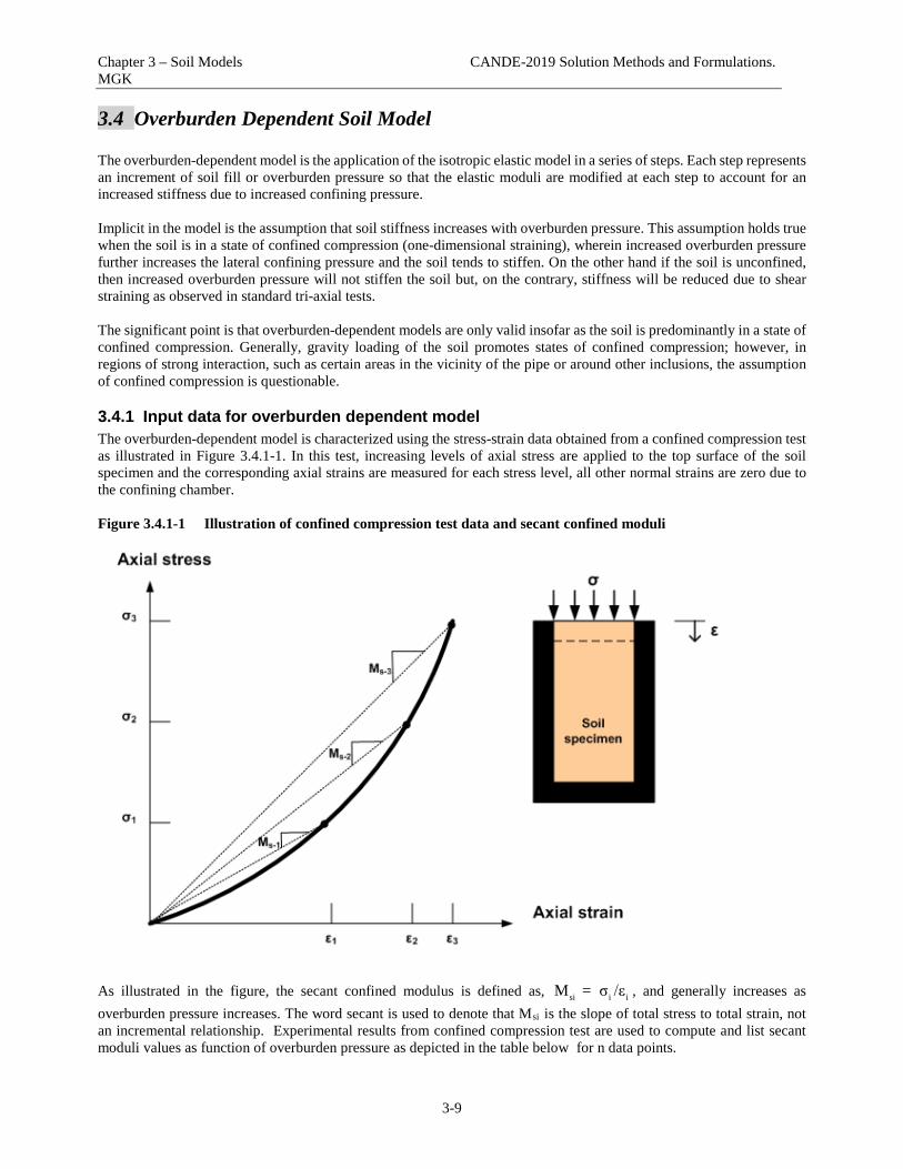
Chapter 3 – Soil Models CANDE-2019 Solution Methods and Formulations. MGK
3-9
3.4 Overburden Dependent Soil Model The overburden-dependent model is the application of the isotropic elastic model in a series of steps. Each step represents an increment of soil fill or overburden pressure so that the elastic moduli are modified at each step to account for an increased stiffness due to increased confining pressure. Implicit in the model is the assumption that soil stiffness increases with overburden pressure. This assumption holds true when the soil is in a state of confined compression (one-dimensional straining), wherein increased overburden pressure further increases the lateral confining pressure and the soil tends to stiffen. On the other hand if the soil is unconfined, then increased overburden pressure will not stiffen the soil but, on the contrary, stiffness will be reduced due to shear straining as observed in standard tri-axial tests. The significant point is that overburden-dependent models are only valid insofar as the soil is predominantly in a state of confined compression. Generally, gravity loading of the soil promotes states of confined compression; however, in regions of strong interaction, such as certain areas in the vicinity of the pipe or around other inclusions, the assumption of confined compression is questionable.
3.4.1 Input data for overburden dependent model The overburden-dependent model is characterized using the stress-strain data obtained from a confined compression test as illustrated in Figure 3.4.1-1. In this test, increasing levels of axial stress are applied to the top surface of the soil specimen and the corresponding axial strains are measured for each stress level, all other normal strains are zero due to the confining chamber. Figure 3.4.1-1 Illustration of confined compression test data and secant confined moduli
As illustrated in the figure, the secant confined modulus is defined as, si i iM = σ /ε , and generally increases as overburden pressure increases. The word secant is used to denote that Msi is the slope of total stress to total strain, not an incremental relationship. Experimental results from confined compression test are used to compute and list secant moduli values as function of overburden pressure as depicted in the table below for n data points.

Chapter 3 – Soil Models CANDE-2019 Solution Methods and Formulations. MGK
3-10
Table 3.4.1-1 Data table of secant moduli versus overburden pressure.
Overburden Pressure (vertical stress)
Secant confined Modulus Msi = σ i/ε i
Secant Young’s modulus Esi = Msi (1+ν)(1-2 ν)/(1- ν)
σ1 Ms1 Es1 σ2 Ms2 Es2 σ3 Ms3 Es3 * * *
* * *
* * *
σn Msn Esn For most soils the lateral soil pressure exerted on the sides of the chamber typically increases in direct proportion to the overburden pressure. Thus the lateral coefficient K0, which is the ratio of lateral pressure to vertical stress, remains practically constant for all levels of vertical stress. Since Poisson ratio ν = K0/(1+ K0), a constant value of Poisson ratio is used to provide the second elastic parameter for the overburden dependent model. Accordingly as shown in the last column of the above table, secant values for Young’s moduli are easily computed by multiplying secant confined moduli by a constant factor β = (1+ν)(1-2 ν)/(1- ν), which is derived from elasticity parameter equivalent relationships (see Table 3.2.1-1). To briefly recap, Table 3.4.1-1 is representative of the data needed to exercise the overburden model in a typical soil-structure problem. CANDE-2019 has “canned tables” of secant Young’s moduli corresponding to increasing values for overburden pressure for typical soils that may be used in lieu of actual test data.
3.4.2 Overburden model development To incorporate the overburden pressure data into the incremental stress-strain relationship, it is necessary to convert the secant moduli data into chord moduli relating increments of vertical stress to increments of vertical strain in going from load step i to step i +1as illustrated in the figure below. Figure 3.4.2-1 Incremental stress-strain relationship and chord modulus
Specifically for each plane-strain element in the soil system, the incremental constitutive matrix has the form,

Chapter 3 – Soil Models CANDE-2019 Solution Methods and Formulations. MGK
3-11
x 11 12 x
y 12 11 y
33
Δσ C C 0 ΔεΔσ = C C 0 ΔεΔτ 0 0 C Δγ
Equation 3.4-1
where C11, C12, and C13 are chord moduli dependent on the stress state at load step i and step i+1. Letting σ i and ε i represent the known vertical stress and strain at load step i in element #n, the increment of vertical stress in element #n is estimated by determining the vertical pressure contributions of all elements above element #n that enter the soil system in load step i+1. Tersely, this is stated as, Δσ ≈ increment of overburden pressure from added soil elements above element #n The algorithm that computes the estimate for Δσ utilizes the finite element mesh topology and element material property data to determines which elements entering the system during load step i+1 are above element #n along with their contributing pressures. The algorithm is laborious but straightforward. Once the estimate for Δσ is obtained, the chord moduli (see above figure) may be determined as,
11i i+1 i
ΔσC = (σ +Δσ)/M - ε
Equation 3.4-2
12 0 11C = K C Equation 3.4-3
33 0 111
2C = (1-K )C Equation 3.4-4
where, σ i , ε i = known stress and strain values in element #n at load step i.
i+1M = secant confined modulus interpolated from data table at pressure σ i + Δσ.
0K = ν/(1- ν) = constant lateral coefficient (ν = Poisson ratio) Herein lies the advantage of an overburden-dependent model over the nonlinear models to be described next. That is, to advance the solution from step i to i+1, the overburden-dependent chord moduli are determined based on the soil layering within the finite element mesh, not on a trial solution. Thus, there are no iterations within the load step and convergence is not an issue with the overburden dependent soil model.
3.4.3 Overburden dependent secant moduli data tables in CANDE For reference, reasonable ranges of Young’s secant moduli are provided in Table 3.4.3-1 along with suggested values for Poisson ratio. The table offers three broad categories of soil; granular, mixed and cohesive for two compaction levels, fair and good. Table 3.4.3-1 – Secant Young’s modulus versus overburden pressure
Soil Class→ Compaction→ MATNAM→
Granular Mixed Cohesive Good Fair Good Fair Good Fair
GGOOD GFAIR MGOOD MFAIR CGOOD CFAIR Overburden
Pressure psi
Young’s Modulus
psi
Young’s Modulus
psi
Young’s Modulus
psi
Young’s Modulus
psi
Young’s Modulus
psi
Young’s Modulus
psi

Chapter 3 – Soil Models CANDE-2019 Solution Methods and Formulations. MGK
3-12
5 1,100 550 600 400 250 150 10 1,300 750 850 550 325 200 15 1,500 850 1,000 600 375 225 20 1,650 1,000 1,100 700 375 250 25 1,800 1,100 1,200 750 400 250 30 1,900 1,150 1,250 800 400 250 40 2,100 1,300 1,350 900 400 250 50 2,250 1,400 1,450 900 400 250
Poisson ratio (pressure
independent)
0.30 to 0.35
0.30 to 0.40
0.33 to 0.40
The above values are a composite of seven different references as well as experimental data from the original CANDE investigation (Reference 1). As a whole the data values are conservative (low side) and are suitable for design if actual soil data is not available.
3.5 Duncan and Duncan/Selig Soil Models The original Duncan and Duncan/Selig soil models are variable-modulus elasticity formulations using stress-dependent equations for Young’s modulus and bulk modulus. The Duncan form and Duncan/Selig form are very similar, differing slightly in the expression for the bulk modulus function. Both forms of the soil models are considered to be very representative of actual soil behavior particularly for representing the stress-dependent behavior of backfill soil in culvert installations. Basically, the models exhibit stiffening of constitutive moduli when confining stress increases and softening when shear stress increases. Duncan’s original work for the Young’s modulus formulation, which is based on a hyperbolic stress-strain relationship, dates back to 1970 (Reference 19) and remains today as originally developed. In 1978 (Reference 20), Duncan and his colleagues introduced a variable bulk modulus to serve as the second constitutive parameter, replacing the previous assumption of a constant Poisson ratio. The bulk modulus function is based on a power law function of confining pressure. Today, Duncan’s original Young’s modulus formulation together with the power-law bulk modulus function is referred to as the Duncan soil model. Selig proposed an alternative form of the bulk modulus function in 1988 (Reference 21). Selig’s bulk modulus function is based on an observed hyperbolic relationship between volumetric strain and hydrostatic pressure from soil specimens in hydrostatic compression. Thus, the so-called Duncan/Selig soil model is based on Duncan’s original Young’s modulus formulation and Selig’s hyperbolic bulk modulus formulation. Selig also performed independent tests to characterize the parameters of the Duncan/Selig model. In 2015 Katona introduced a Modified form of Duncan and Duncan/Selig soil models to simulate plastic-like behavior with permanent deformation upon unloading (Reference 29). That is, although the original model is excellent in tracking the nonlinear behavior of soils in loading environments, it retraces the same stress-strain path upon unloading. Consequently, the original model does not predict residual deformation, which is invariably observed in laboratory soil specimens following a load-unload cycle. The new modified Duncan/Selig model produces permanent deformations upon unloading similar to advanced plasticity models. No new material parameters are introduced into the modified formulation; thus, the large existing data base of Duncan/Selig parameters remains valid for the modified formulation. In the following sections, the original Duncan and Duncan/Selig models are presented first followed by the Katona modification given in the last section. The CANDE-2019 computer program provides the option to “turn on” or “turn off” the modified formulation at the user’s discretion.
3.5.1 Plane-strain constitutive matrix From an overall perspective, the Duncan and the Duncan/Selig soil models are used to define the nonlinear components of an isotropic, elasticity-based constitutive matrix for plane-strain conditions as expressed below.

Chapter 3 – Soil Models CANDE-2019 Solution Methods and Formulations. MGK
3-13
x 11 12 x
y 12 11 y
33
Δσ C C 0 ΔεΔσ = C C 0 ΔεΔτ 0 0 C Δγ
Equation 3.5-1
where, x yΔσ , Δσ , Δτ = stress increments for x-direction, y-direction and shear components, respectively
x yΔε , Δε , Δγ = strain increments for x-direction, y-direction and shear components, respectively
11 12 33C , C , C = nonlinear coefficients dependent on Young’s modulus and bulk modulus functions. The table below shows the relationship between the constitutive matrix components and the elastic functions. Table 3.5.1-1 Components for constitutive matrix relationship to moduli functions
Components of Constitutive matrix
E = Young’s modulus
B = bulk modulus (E, B)
E = Young’s modulus
ν = Poisson ratio (E, ν)
C11 =
3B(3B + E)
9B - E
( )
( )( )E 1- ν
1+ ν 1-2ν
C12 =
3B(3B - E)
9B - E
( )( )Eν
1+ ν 1-2ν
C33 =
3BE
9B - E
( )E
2 1+ ν
The middle column in the above table defines the matrix coefficients C11, C12 and C13 in terms of Young’s modulus and bulk modulus, which are the elastic parameter functions developed in the current Duncan and Duncan Selig models. The third column defines the matrix coefficients in terms of Young’s modulus and Poisson ratio, which was the 1970 form of the Duncan model. We will return to the implications of the constitutive matrix after the functional forms of Young’s modulus and bulk modulus are presented.
3.5.2 Duncan Young’s modulus development Duncan’s formulation is based on experimental observations of soil behavior from standard tri-axial tests. A standard tri-axial test is conducted by placing a cylindrical soil specimen in a pressure chamber and initially subjecting the specimen to a uniform hydrostatic pressure, called σ3. Next a steadily increasing axial load is applied to the specimen producing a net axial stress, called σ1, which includes the hydrostatic pressure. Note that σ3 and σ1 are principal stresses in the lateral and axial directions, respectively. The difference in principal stresses σ1 – σ3 is called the deviator stress and is equal to twice the maximum shear stress occurring on 45-degree plane. As the axial stress increases, axial strain is computed by measuring the axial shortening of the specimen divided by the specimen length. Note the measured axial strain does not include the initial hydrostatic strain. The dashed curve in Figure 3.5.2-1 is a plot of deviator stress versus axial strain for a typical tri-axial test. Here, (σ1 – σ3) f is the measured maximum deviator stress at failure, and Ei is the initial slope representing Young’s modulus at zero deviator stress. As discussed subsequently, (σ1 – σ3) f and Ei are dependent on the hydrostatic stress level. Figure 3.5.2-1 Deviator stress versus axial strain for tri-axial test and hyperbolic approximation
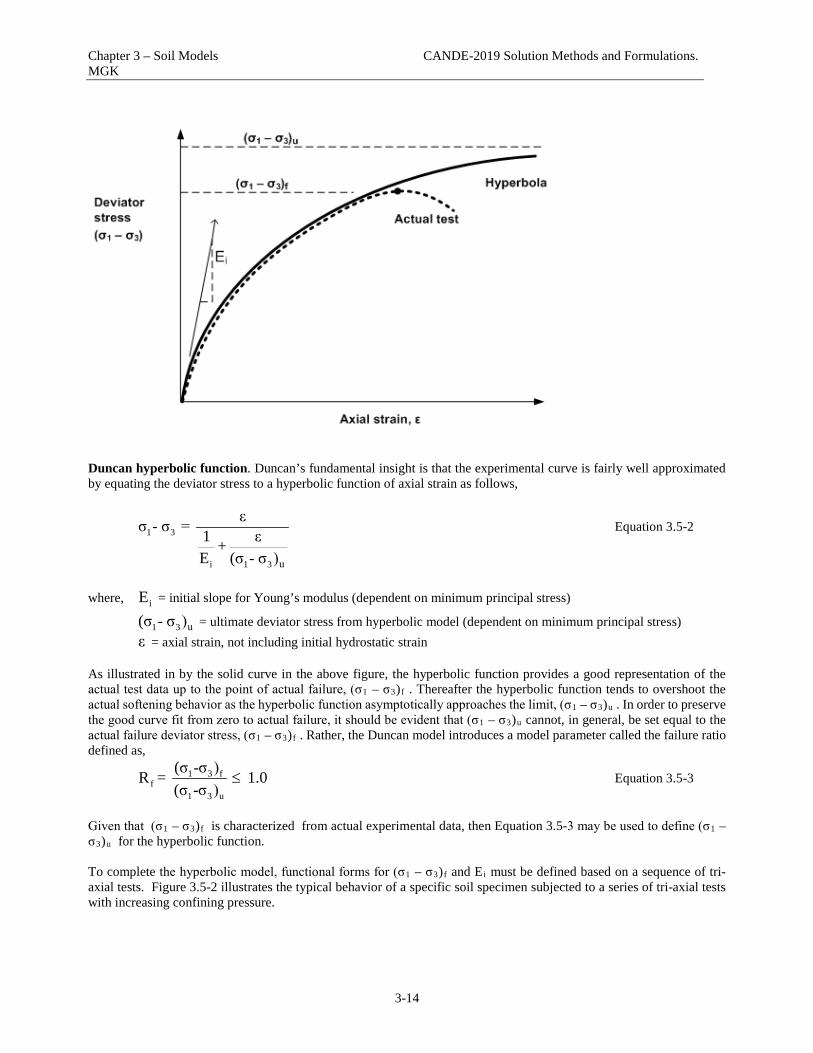
Chapter 3 – Soil Models CANDE-2019 Solution Methods and Formulations. MGK
3-14
Duncan hyperbolic function. Duncan’s fundamental insight is that the experimental curve is fairly well approximated by equating the deviator stress to a hyperbolic function of axial strain as follows,
1 3
i 1 3 u
εσ - σ = 1 ε+E (σ - σ )
Equation 3.5-2
where, iE = initial slope for Young’s modulus (dependent on minimum principal stress)
1 3 u(σ - σ ) = ultimate deviator stress from hyperbolic model (dependent on minimum principal stress) ε = axial strain, not including initial hydrostatic strain As illustrated in by the solid curve in the above figure, the hyperbolic function provides a good representation of the actual test data up to the point of actual failure, (σ1 – σ3)f . Thereafter the hyperbolic function tends to overshoot the actual softening behavior as the hyperbolic function asymptotically approaches the limit, (σ1 – σ3)u . In order to preserve the good curve fit from zero to actual failure, it should be evident that (σ1 – σ3)u cannot, in general, be set equal to the actual failure deviator stress, (σ1 – σ3)f . Rather, the Duncan model introduces a model parameter called the failure ratio defined as,
1 3 ff
1 3 u
(σ -σ )R = 1.0(σ -σ )
≤ Equation 3.5-3
Given that (σ1 – σ3)f is characterized from actual experimental data, then Equation 3.5-3 may be used to define (σ1 – σ3)u for the hyperbolic function. To complete the hyperbolic model, functional forms for (σ1 – σ3)f and Ei must be defined based on a sequence of tri-axial tests. Figure 3.5-2 illustrates the typical behavior of a specific soil specimen subjected to a series of tri-axial tests with increasing confining pressure.

Chapter 3 – Soil Models CANDE-2019 Solution Methods and Formulations. MGK
3-15
Figure 3.5.2-2 Typical behavior of a soil specimen in a sequence of tri-axial tests.
Initial Young’s modulus. Based on a wide variety of soil tests as typified by the above figure, the initial modulus is observed to increase with confining pressure according to the following power law,
ni a 3 aE = KP (σ /P ) Equation 3.5-4
where, iE = initial Young’s modulus when deviator stress = 0
K = dimensionless magnitude of initial Young’s modulus aP = atmospheric pressure used to nondimensionalize parameters K and n n = power-law coefficient usually less than 1.0 3σ = confining pressure, minimum magnitude of principle stress Mohr-Coulomb failure envelope. As portrayed in the Figure 3.5-2, the deviator stress at failure increases with confining pressure. Based on the well-known Mohr-Coulomb failure theory, the (σ1 – σ3)f i data points define a failure envelope in terms of normal stress and shear stress as depicted in the figure below. Figure 3.5.2-3 Failure envelope in normal and shear stress space

Chapter 3 – Soil Models CANDE-2019 Solution Methods and Formulations. MGK
3-16
Typically, the Mohr-Coulomb failure surface is a straight line defined by two constants, C and φ0, representing the cohesion intercept and a constant soil friction angle, respectively. As illustrated in the above figure, a more general form of the Mohr-Coulomb failure surface is used in this development wherein the soil friction angle is a decreasing function of the confining pressure. Often, this is a better representation of actual soil behavior. Based on the generalized Mohr-Coulomb theory, the tri-axial deviator stress at failure is characterized as follows,
31 3 f
2C cosφ + 2σ sinφ(σ - σ ) = 1- sinφ
Equation 3.5-5
where, 0 10 3 aφ = φ - Δφ log (σ /P ) = variable soil friction angle Equation 3.5-6
C = cohesion intercept, units of stress 0φ = Reference soil friction angle at σ3/Pa = 1
Δφ = reduction of soil friction angle for 10-fold increase in σ3
Tangent Young’s modulus. Tangent Young’s modulus is equal to the derivative of axial stress to axial strain under the conditions of tri-axial testing wherein the confining stress is constant. Since all the terms are now identified in Equation 3.5-2, we can compute tangent Young’s modulus by forming the derivative dσ1/dε and replacing strain values with equivalent stresses via Equation 3.5-2 to arrive at,
2f 1 3t i
3
R (1- sinφ)(σ - σ )E = E 1 - 2(Ccosφ + σ sinφ)
[ ] Equation 3.5-7
where, tE = tangent Young’s modulus dependent on stress state
1σ = maximum compressive principal stress
3σ = minimum compressive principal stress Equation 3.5.7 is fundamental for both the Duncan soil model and the Duncan/Selig soil model.
3.5.3 Bulk modulus formulations By definition, the tangent bulk modulus is the change in mean stress divided by the change in volumetric strain, which is expressed as
mt
vol
dσB = dε
Equation 3.5-8

Chapter 3 – Soil Models CANDE-2019 Solution Methods and Formulations. MGK
3-17
where, tB = tangent bulk modulus, usually stress dependent for soils.
m 11 22 33σ = (σ + σ + σ )/3 = mean average stress, also called hydrostatic stress
vol 0 11 22 33ε = dV/V = ε + ε + ε = volumetric strain Duncan bulk modulus function. Duncan used tri-axial test data including measurements of volumetric strain to obtain experimental values for the tangent bulk modulus computed as,
measured axial vol1B = Δσ /Δε3
Equation 3.5-9
For a given confining pressure, the change in axial stress and corresponding change in volumetric strain are measured when the axial stress reaches 70% of the failure stress or the volumetric strain peaks in contraction, whichever occurs first. Based on a series of tri-axial tests with increasing confining pressure, Duncan proposed a power-law function (very similar to the initial Young’s modulus function) to describe the tangent bulk modulus as, m
t b a 3 aB = K P (σ /P ) Equation 3.5-10 where, bK = dimensionless magnitude of tangent bulk modulus
aP = atmospheric pressure used to nondimensionalize parameters Kb and m m = power-law coefficient usually less than 1.0 3σ = confining pressure or minimum magnitude of principle stress Selig bulk modulus function. Selig developed an alternate form of the tangent bulk modulus function based on hydrostatic tests. In the hydrostatic test the soil specimen is compressed under increasing confining pressure applied equally in all directions and the change of volume is measured as function of confining pressure as depicted in the figure below. Figure 3.5.3-1 Hydrostatic test and Selig’s hyperbolic model
Selig observed that the experimental curves relating mean stress to volumetric strain is reasonably described by a hyperbolic equation in the form,
σm
σmσm
σm
V
V0
ΔV = V-V0
Mean stress σm
εvol = ΔV/V0εu
Bt

Chapter 3 – Soil Models CANDE-2019 Solution Methods and Formulations. MGK
3-18
im vol
vol u
Bσ = ( )ε1 - ε /ε
Equation 3.5-11
where, iB = initial tangent bulk modulus when volumetric strain = 0.
uε = ultimate volumetric strain at large hydrostatic stress. As illustrated in Figure 3.5.3-1, the tangent bulk modulus is determined by forming the derivative dσm/dεvol and again using Equation 3.5-11 to replace volumetric strain with hydrostatic stress to get the final result, 2
t i m i uB = B [1+ σ /(B ε )] Equation 3.5-12
where, tB = Selig form of tangent bulk modulus dependent on mean hydrostatic stress.
3.5.4 Summary of Original Duncan and Duncan/Selig soil models. To summarize the tangent Young’s modulus function, Equation 3.5-7 is written in a more compact form as shown by Equation 3.5-13.
td
idMax
2σE = E 1 - σ
[ ] Equation 3.5-13
Where, n3i a
a
σE = KP ( )P
Equation 3.5-14
f
dMax32 Ccos + sin( )
(=
R 1- si )nσ
σφ φφ
Equation 3.5-15
0 10 3 aφ = φ - Δφ log (σ /P ) Equation 3.5-16
Definitions of the symbols are listed below. • tE = tangent Young’s modulus dependent on complete stress state,
• iE = initial Young’s modulus dependent on minimum compressive stress, • σdMax = Maximum deviatoric stress at failure
• φ = angle of internal friction dependent on minimum compressive stress,
• 1σ = maximum compressive principal stress,
• 3σ = minimum compressive principal stress,
• aP = atmospheric pressure, a constant for units of stress. Material properties required for the above tangent young’s modulus functions are,
• K = dimensionless magnitude of initial Young’s modulus, • n = power-law coefficient for initial modulus usually less than 1.0, • C = cohesion intercept for failure, units of stress, • 0φ = initial soil friction angle of failure surface,
• Δφ = reduction of soil friction angle for 10-fold increase in σ3,
• fR = failure ratio of actual to model failure stress usually less than 1.0.

Chapter 3 – Soil Models CANDE-2019 Solution Methods and Formulations. MGK
3-19
For the second elasticity function, the choice is between Duncan’s tangent bulk modulus power law or Selig’s tangent bulk modulus derived from a hyperbolic relationship between hydrostatic pressure and volumetric strain. Duncan’s tangent bulk modulus power-law function is given by, m
t b a 3 aB = K P (σ /P ) Equation 3.5-17a Material properties required for Duncan’s tangent bulk modulus power law are,
• bK = dimensionless magnitude of tangent bulk modulus, • m = power-law coefficient usually less than 1.0.
Alternatively, Selig’s tangent bulk modulus function is written compactly as,
mt i
mRef
2σB = B 1+ [ ]
σ Equation 3.5-17b
where, 1m 2 3σ +1σ = σ + ( σ )3
= average principle stress.
and, umRef iσ = B ε = reference stress (a constant) Material properties required for Selig’s tangent bulk modulus function are, iB = initial tangent bulk modulus when hydrostatic stress is zero,
uε = ultimate volumetric strain at large hydrostatic stress. See Section 3.58 for plastic-like unload/reload formulations.
3.5.5 Behavioral characteristics and special considerations The behavioral characteristics and limitations of the Duncan and the Duncan/Selig soil model are nearly identical and are enumerated below along with discussions on special treatments for limiting cases. Recall that maximum shear stress is equal to half the difference in principal stresses, (σ1 – σ3)/2.
• If confining pressure increases while shear stress is held constant, Et and Bt become stiffer. However if maximum shear increases with constant confining pressure, Et becomes softer while Bt remains constant.
• Shear failure is said to occur when Et approaches zero as shear stress increases to the failure limit. To avoid
numerical problems, the bracketed term in Equation 3.5-13, which varies from 1.0 to 0.0 as shear stress increases, is limited to the minimum value 0.05 so that Et = 0.0025Ei is the minimum tangent Young’s modulus, which is effectively a near-zero stiffness.
• Tension failure is said to occur when the minimum compressive stress σ3 becomes tensile wherein most soils
breakdown and lose all stiffness. This is simulated in the soil models by assigning a small limiting value to the minimum compressive stress, σ3/Pa = 0.1, so that Et and Bt are near-zero stiffness values whenever the minimum principal stress approaches tension.
• Although Et and Bt are developed as two independent functions, energy considerations require constraints
between the functions (e.g. see Table 3.5-1). The soil models programmed in CANDE satisfy the energy constraints by enforcing,
Et > 0, and Et/3 < Bt < 8Et.
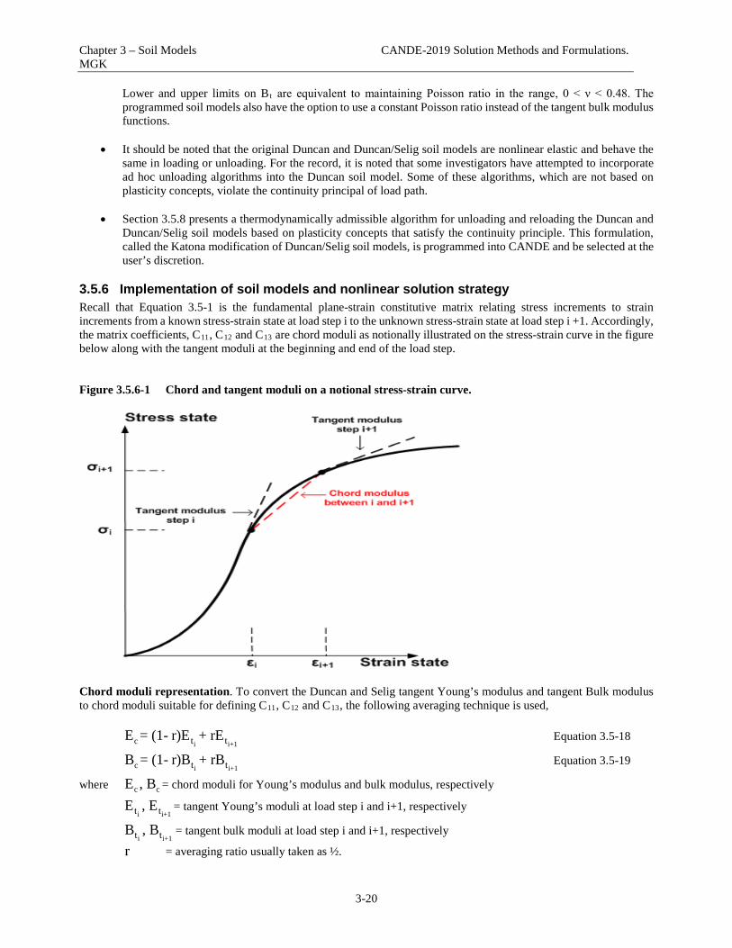
Chapter 3 – Soil Models CANDE-2019 Solution Methods and Formulations. MGK
3-20
Lower and upper limits on Bt are equivalent to maintaining Poisson ratio in the range, 0 < ν < 0.48. The programmed soil models also have the option to use a constant Poisson ratio instead of the tangent bulk modulus functions.
• It should be noted that the original Duncan and Duncan/Selig soil models are nonlinear elastic and behave the
same in loading or unloading. For the record, it is noted that some investigators have attempted to incorporate ad hoc unloading algorithms into the Duncan soil model. Some of these algorithms, which are not based on plasticity concepts, violate the continuity principal of load path.
• Section 3.5.8 presents a thermodynamically admissible algorithm for unloading and reloading the Duncan and Duncan/Selig soil models based on plasticity concepts that satisfy the continuity principle. This formulation, called the Katona modification of Duncan/Selig soil models, is programmed into CANDE and be selected at the user’s discretion.
3.5.6 Implementation of soil models and nonlinear solution strategy Recall that Equation 3.5-1 is the fundamental plane-strain constitutive matrix relating stress increments to strain increments from a known stress-strain state at load step i to the unknown stress-strain state at load step i +1. Accordingly, the matrix coefficients, C11, C12 and C13 are chord moduli as notionally illustrated on the stress-strain curve in the figure below along with the tangent moduli at the beginning and end of the load step. Figure 3.5.6-1 Chord and tangent moduli on a notional stress-strain curve.
Chord moduli representation. To convert the Duncan and Selig tangent Young’s modulus and tangent Bulk modulus to chord moduli suitable for defining C11, C12 and C13, the following averaging technique is used,
i i+1c t tE = (1- r)E + rE Equation 3.5-18
i i+1c t tB = (1- r)B + rB Equation 3.5-19
where c cE , B = chord moduli for Young’s modulus and bulk modulus, respectively
i i+1t tE , E = tangent Young’s moduli at load step i and i+1, respectively
i i+1t tB , B = tangent bulk moduli at load step i and i+1, respectively
r = averaging ratio usually taken as ½.

Chapter 3 – Soil Models CANDE-2019 Solution Methods and Formulations. MGK
3-21
The justification for averaging the tangent moduli to obtain the chord moduli follows from the mean-value-theorem of differential calculus, which implies that the process becomes exact as the size of the load step decreases. Generally the averaging ratio is taken as r = ½. However as explained in the next paragraph, it is reasonable to set r =1when in situ soil elements enter the structural system for the first time. For this reason, the averaging ratio is treated as a material input parameter. Entering soil elements. Soil elements enter the structural system in one of two categories. The first category applies to pre-existing or in-situ soil elements in which an initial state of stress exists but is generally not known prior to the solution. Elements entering in this category are typically part of the initial configuration and are assigned to the first construction increment. The second category applies to fill soi1 elements, i.e., soil layers added to the system in a predefined construction schedule. Here, the initial stress state is non-existent prior to entry into the system. Both categories present special starting problems for the iteration scheme because the initial stress state is unknown in the first category or nonexistent in the second category. For the first category, the initial stress state can be determined iteratively by assuming the pre-existing soil zone is a construction increment loaded with its own body weight (and, if desired, a consolidation pressure). In this case the averaging ratio should be set to 1.0, so that, Ec and Bc are equal to the tangent values at the end of the load step because this corresponds to the existing stress state. When r = 1, the tangent moduli at the beginning of the load step have no influence on the averaging process. After the first construction increment is complete, the algorithm automatically changes r = 1/2 so that all subsequent moduli calculations represent chord values in going from a known stress state to an unknown stress state. For the second category, soil layers entering the system for the first time have zero initial stress and zero initial stiffness at the beginning of the load step but gain stiffness at the end of the load step from self-weight and/or compaction load. In this case, using r = 1/2 implies the effective chord moduli during the load step is equal to one-half the tangent moduli at the end of the load step, which is considered to be a reasonable assumption. For all load steps following the initial load step, there is no longer any ambiguity and we set r =1/2 because we know the stress state at the start of each subsequent load step. To start the iteration process for entering elements of either category, some initial guess must be made for the end-of-load-step tangent moduli because the start-of-load step moduli are zero. Thus in order to construct the first trial stiffness matrix, "dummy" principle stresses are used to get the first trial moduli value. The dummy principle stresses have no effect on the final converged solution, but they do influence the number of iterations required to achieve convergence. After an element has entered the system, the initial guess for end-of-load-step tangent moduli for all subsequent load steps are equated to the last calculated values and the use of dummy principal stresses is not required. Nonlinear solution summary. Based on the forgoing discussion, a summary on the nonlinear solution strategy is provided in the flowchart shown in Figure 3.5.6-2. The flow chart depicts the iteration cycle to determine the constitutive matrix of a soil element wherein the principal stresses from the last iteration are used make closer and closer estimates of the chord moduli until convergence occurs. Convergence of the algorithm occurs when the chord moduli obtained from two successive iterations differ by no more than 1% for all elements. Two additional features of the algorithm not shown in the flow chart are listed below.
1. An under-relaxation scheme to improve the rate of convergence for the tangent moduli comes into play after the second iteration wherein each estimate of the end-of-load-step tangent moduli is a weighted average of the current estimate and the previous iteration estimate. This feature takes advantage of the observation that convergence occurs in an oscillatory manner.
2. A constant Poisson ratio option may be chosen by the user that replaces the tangent bulk modulus formulation.
When the constant Poisson ratio option is exercised, the bulk modulus formulations are bypassed. Otherwise, the algorithm is essentially the same.

Chapter 3 – Soil Models CANDE-2019 Solution Methods and Formulations. MGK
3-22
Figure 3.5.6-2 Duncan and Duncan/Selig flow chart for computing constitutive matrix.

Chapter 3 – Soil Models CANDE-2019 Solution Methods and Formulations. MGK
3-23
3.5.7 Recommended Duncan and Duncan/Selig parameters for standard soils Whenever possible, the Duncan and/or Duncan Selig soil model parameters should be determined directly from tri-axial test equipment using established curve-fitting procedures. In many instances, however, tri-axial data may be unavailable, and so, it is convenient to establish standard parameter values for various types of soil and degrees of compaction. Table 3.5.7-1 provides parameter values for the Duncan soil model for four soil classifications, each with three levels of compaction. These standard values, extracted from References 19 and 20, are conservative in the sense that they are the lower bounds of strength and moduli values observed from numerous tri-axial tests for each soil type. An independent study at the University of Notre Dame utilizing the same database verified that the table parameters give a good but conservative representation of the experimental data. Table 3.5.7-1 Duncan soil model parameters (from Duncan Reference
Soil type and compaction
Young’s Tangent Modulus Parameters Bulk Parameters Density reference
(lb/ft3) K n C φ0 Δφ Rf Kb m
(--) (--) (psi) (deg) (deg) (--) (--) (--) CA105 600 0.40 0.0 42 9 0.7 175 0.2 150 CA95 300 0.40 0.0 36 5 0.7 75 0.2 140 CA90 200 0.40 0.0 33 3 0.7 50 0.2 135 SM100 600 0.25 0.0 36 8 0.7 450 0.0 135 SM90 300 0.25 0.0 32 4 0.7 250 0.0 125 SM85 150 0.25 0.0 30 2 0.7 150 0.0 120 SC100 400 0.60 0.5 33 0 0.7 200 0.5 135 SC90 150 0.60 0.3 33 0 0.7 75 0.5 125 SC85 100 0.60 0.2 33 0 0.7 50 0.5 120 CL100 150 0.45 0.4 30 0 0.7 140 0.2 135 CL90 90 0.45 0.2 30 0 0.7 80 0.2 125 CL85 60 0.45 0.1 30 0 0.7 50 0.2 120
In the above table the soil type is defined as follows: CA = Course Aggregates, SM = Silty Sand, SC = Silty-Clayey Sand and CL = Silty Clay. The compaction number is percent relative compaction, per AASHTO T-99. As an example, SM100 means silty sand compacted to 100% relative density per T-99. In a similar manner Table 3.5.7-2 provides parameter values for the Duncan/Selig soil model for three soil classifications, each with five levels of compaction. These values were computed by Selig in Reference 21 and are generally conservative. The bulk modulus parameters were determined from hydrostatic tests which, according to Selig, tend to be more conservative than those determined from standard tri-axial tests.

Chapter 3 – Soil Models CANDE-2019 Solution Methods and Formulations. MGK
3-24
Table 3.5.7-2 Duncan/Selig soil model parameters (from Selig Reference) Soil type and compaction
Young’s Tangent Modulus Parameters Bulk Parameters Density reference
(lb/ft3) K n C φ0 Δφ Rf Bi/ Pa ε u
(--) (--) (psi) (deg) (deg) (--) (--) (--) SW100 1300 0.90 0.0 54 15 0.65 108.8 0.01 148 SW95 950 0.60 0.0 48 8.0 0.70 74.8 0.02 145 SW90 640 0.43 0.0 42 4.0 0.75 40.8 0.05 140 SW85 450 0.35 0.0 38 2.0 0.80 12.7 0.08 130 SW80 320 0.35 0.0 36 1.0 0.90 6.1 0.11 120 ML95 440 0.40 4.0 34 0.0 0.95 48.3 0.06 135 ML90 200 0.26 3.5 32 0.0 0.89 18.4 0.10 130 ML85 110 0.25 3.0 30 0.0 0.85 9.5 0.14 122 ML80 75 0.25 2.5 28 0.0 0.80 5.1 0.19 115 ML50 16 0.95 0.0 23 0.0 0.55 1.3 0.43 66 CL95 120 0.45 9.0 15 4.0 1.00 21.2 0.13 130 CL90 75 0.54 7.0 17 7.0 0.94 10.2 0.17 125 CL85 50 0.60 6.0 18 8.0 0.90 5.2 0.21 120 CL80 35 0.66 5.0 19 8.5 0.87 3.5 0.25 112
In the above table the soil type is defined as follows: SW = Gravelly sand, ML = Sandy silt, and CL = Silty Clay. The compaction number is percent relative compaction, per AASHTO T-99. As an example, SW95 means gravelly sand compacted to 95% relative density per T-99. In the old CANDE-1989 documentation, Selig presented less conservative values for the tangent bulk modulus parameters by uniformly increasing the parameter Bi/Pa by a factor of 2.5 and uniformly decreasing εu by the factor 0.71. However, in recent years most researchers prefer the original hydrostatic data given in the above table.
3.5.8 Modified Duncan/Selig models for plastic deformation (Katona) The Original Duncan and Duncan/Selig formulation is a nonlinear elastic model that travels the same stress-strain path in loading and unloading. Although the original model does an excellent job in capturing the nonlinear loading behavior, actual soil samples exhibit linear-like unloading and reloading similar to some plasticity-based constitutive models. In particular, the so-called PLAXIS soil hardening model employs a plasticity-based hardening rule that was developed to mimic the Duncan/Selig variable-modulus model under loading conditions along with elastic unloading and reloading behavior (Reference 30). One short coming of the PLAXIS model is that it requires new model material parameters that are not defined in the existing Duncan/Selig data base for typical soils and levels of compaction. Clearly it is a desirable objective to modify the Duncan/Selig soil model to simulate the observed plastic-like behavior of soils in unloading and reloading conditions without introducing additional model parameters and retaining the variable modulus formulation. Specifically the objective is to modify the model to unload and reload with appropriate linear elastic stiffness and to establish the criteria to define loading stress space versus unload/reload stress space. Underlying this objective is the requirement to prove that the modified model meets all thermodynamic restrictions for constitutive theories. To achieve the objective, concepts from advanced plasticity theory are introduced into the original Duncan/Selig formulation such as stress-dependent history variables. However, the modified Duncan/Selig model remains a variable modulus formulation without explicitly dividing the strain into elastic and plastic components. The proposed formulation must satisfy thermodynamic restrictions, which under the assumptions of time and temperature independence, are reduced to the following two requirements:
1. Positive work. Work must be positive during any load increment without creation of energy during any load cycle. In this study it is shown that the modified Duncan/Selig formulation satisfies Drucker’s postulate, which is a sufficient condition to satisfy this thermodynamic requirement.

Chapter 3 – Soil Models CANDE-2019 Solution Methods and Formulations. MGK
3-25
2. Stress-strain continuity. Infinitesimal changes in the orientation of an incremental stress vector must result in small changes in the incremental strain vector; i.e., no discontinuous jumps in strain magnitude. In this study a plasticity-like normality factor is introduced into the variable Young’s modulus function in order to satisfy the continuity requirement.
Young’s Modulus Loading/Unloading Modification. To satisfy the stress-strain continuity requirement, Equation 3.5-13 is modified by inserting a continuity factor called β, where 0 ≤ β ≤ 1, as defined below.
td
idMax
2σE = E 1 - σ
[ ]β Equation 3.5-20
d
2 2d 3
Δσ = Maximum ( , 0 )
Δσ +Δσβ Equation 3.5-21
The continuity factor is similar to the consistency condition in plasticity theory that asserts the growth of the yield surface is proportional to the applied stress vector acting in the direction normal to yield surface (dot product). To illustrate how the continuity factor accounts for loading and unloading consider the two stress paths shown in the figure below. Figure 3.5.8-1. Illustration of load/unload stress paths for tri-axial and arbitrary conditions.
First consider the standard tri-axial stress path shown on the left side of the above figure wherein deviatoric load increments Δσd are shown with vertical black arrows (since Δσ3 = 0). For each of these loading steps, Equation 3.5-21 gives β = Δσd/│ Δσd│ = 1. Therefore the tangent Young’s modulus represents a pure loading condition exactly according to the original formulation, Equation 3.5-13, wherein the stiffness is decreasing. However, the fourth load increment
Δσd
Δσ3
θ
0.8
0.6
0.4
0.2
0.0
1.0
Minimum compressive stress , σ3 →
Standard tri-axial stress path: • σ3 held constant (σ0)• Load/unload with Δσd
↓
Arbitrary stress path: ↓
σ0
Dev
iato
ric s
tres
s ra
tio ,
σ d /
σ dM
ax

Chapter 3 – Soil Models CANDE-2019 Solution Methods and Formulations. MGK
3-26
shown with the red arrow is unloading (negative increment) so that we find - Δσd/│ Δσd│ = -1, which means β = 0. Therefore the tangent Young’s modulus becomes Et = Ei satisfying the objective to unload elastically with the initial stiffness function. It is important to realize that the reversal of stress at step 4 constitutes a “large” change in orientation because the direction of the stress vector is turned 180 degrees. Consequently the abrupt change in stiffness from loading (Et << Ei) to unloading (Et= Ei) does not violate the continuity principle because the stress reversal is a “large” change in loading direction. To demonstrate the continuity principle is satisfied for small changes in stress, consider the arbitrary stress path shown on the right side of Figure 3.5.5-1. Here each of the four load steps is associated with an arbitrary incremental stress vector with components Δσ3 , Δσd that define an angle θ as illustrated in the last load step shown in red. Since β = cos θ when θ is between -90 degrees and + 90 degrees, it is evident that a “small” change in θ from load step to load step will produce a small change in β and, hence a small change in the stiffness function; thereby satisfying the continuity requirement. Based on the above concepts, loading and unloading definitions are summarized in the table below where it is observed the stiffness increases smoothly from the maximum loading angle θ = 0 degrees to the neutral loading angles θ = ± 90 degrees. Table 3.5.8-1. Loading definitions dependent on angle of stress-components θ
Loading Definitions
( )-1 d
1/22 2d 3
Δσθ = cos
Δσ + Δσ
β
Normality factor
E
Tangent Young’s Modulus
Maximum loading
θ = 00
β = 1
di
dMax
2σE = E 1 - σ
[ ]
Intermediate loading
-900 < θ < 900
0 < β =cosθ < 1
di
dMax
2σE = E 1 - σ
[ ]β
Neutral loading
θ = ± 900
β = 0
E = Ei
Unloading
│θ│ > 900
β = 0
E = Ei
Unload/Reload Range. Next we need to establish the stress range wherein the initial elastic modulus Ei function is used for further unloading or reloading steps. This problem is solved by borrowing another plasticity concept called “isotropic hardening” that defines a load-history variable that tracks the largest growth of the yield surface over all past loading steps to present. In accordance with the original Duncan formulation, the yield function is the deviatoric stress. Therefore, we define the load-history variable z (n) to track the largest deviatoric stress obtained over load steps 1, 2, n, where n is the current load step number. Starting with z (0) = 0, the load-history variable is updated at the end of each converged load step as shown below. (n) (n-1) d(n)z = Max (z , σ ) Equation 3.5-22 Note that z(n) increases if and only if load-step n results in a deviatoric stress greater than the previous high value; otherwise, z(n) does not change in value. Thus z(n) defines the current boundary separating the linear unload/reload domain from the nonlinear loading domain. During the iterative solution process for load step n+1, the trial solution σd(n+1) is compared with z(n) to determine the appropriate equation for tangent Young’s modulus for the next iteration as shown below.

Chapter 3 – Soil Models CANDE-2019 Solution Methods and Formulations. MGK
3-27
( ) (n) (nd n +1)+1d
idMax
2If > z , then E = (loading domainσ )σ E 1 -
σ[ ]β Equation 3.5-23a
( ) ( )d n+1 (n+1) i z , then E = E (unload/reload domain, If 0)σ =n β≤ Equation 3.5-23b
When operating in the unload/reload elastic domain, the initial modulus function Ei (Equation 3.5-4) is evaluated with the minimum stress value σ3* that is associated with the stress state of z(n). In other words, σ3* is a second load-history variable that is saved along with z(n). Thus, Ei is constant value for a specific unload/reload cycle. Effective Young’s Modulus. By definition En and En+1 are the tangent modulus values at the end of load steps n and n+1, respectively. The effective modulus value Eeffective assigned to the incremental stress-strain matrix (Equation 3.5-1) is an appropriate weighted average of these two values depending on loading/unloading conditions as shown in the equation below with the weighted averaging ratio rE defined in Table 3.5.8-2. effective E (n) E (n+1)E = (1- r ) E + r E Equation 3.5-24 Table 3.5.8-2 Weighted averaging ratio (0 ≤ r E ≤ 1) as defined below.
Loading Conditions
rE value
Criteria for condition
(1) Pure loading 1/2 (n) d(n) d(n+1) d(n)z = σ and σ - σ > 0
(2) Pure unloading 1/2 (n) d(n) d(n+1) d(n)z > σ and σ - σ < 0
(3) Load-to-unload transition 1 (n) d(n) d(n+1) d(n)z = σ and σ - σ < 0
(4) Reload-to-load transition d(n+1) (n)E
d(n+1) d(n)
σ - zr =
σ - σ (n) d(n) d(n+1) (n)z > σ and σ > z
The above table applies to all iterations while solving for incremental stresses from load-step n to n+1 until convergence is achieved. For loading conditions 1 and 2, the averaging ratio is ½, which places equal weight on the beginning and ending tangent moduli in conformance with the mean value theorem of calculus for smooth functions. Case 3 places the total weight on the ending modulus (elastic) in order to simulate the abrupt change in stiffness upon load reversal. Finally, case 4 assigns rE equal to the proportion of the stress increment that exceeds the linear range; conversely, (1-rE) is the proportion within the linear range. These weights generate an accurate stress-strain response for all load/unload/reload conditions. Bulk Modulus Loading/Unloading Modification. The bulk modulus function, either the power law form (Equation 3.5-17a) or the hyperbolic form (Equation3.5-17b) monotonically increases in value during hydrostatic loading conditions. That is, the bulk modulus becomes steadily stiffer as the hydrostatic stress increases, which is in accordance with experimental observations. Upon unloading, however, experimental evidence indicates that the response is linear with a constant bulk modulus approximately equal to the current tangent bulk modulus of the loading curve. Thus the proposed modification to the original bulk modulus function is to unload and reload with a constant bulk modulus equal to the tangent of the loading curve. Based on the above, the proposed bulk modulus formulation inherently satisfies the continuity principle because the loading, unloading and reloading bulk modulus values are identical at the common point of departure/return on the loading curve. Therefore, the bulk modulus loading function, Equation 3.5-17a or b, does not need to be modified as was required for the Young’s modulus function with the insertion of a continuity factor. Bulk Modulus Unload/Reload Range. Similar to the Young’s modulus formulation, we need to establish and track the current stress range wherein the linear bulk modulus remains valid for subsequent unloading or reloading steps. Here

Chapter 3 – Soil Models CANDE-2019 Solution Methods and Formulations. MGK
3-28
again we use the plasticity concept of a load history variable q(n) representing the largest historical value of average stress σm or minimum stress σ3, depending on whether the Selig or Duncan bulk modulus function is selected. The following equations are for the Selig bulk modulus function with the understanding that the Duncan form is very similar. Starting with q(0) = 0, the load-history variable is updated at the end of each converged load-step n as shown below. (n) (n-1) m(n)q = Max(q , σ ) Equation 3.5-25 The variable q(n) increases if and only if load-step n results in a positive loading increment of average stress; otherwise, q(n) does not change in value. Thus q(n) defines the current average-stress level separating the unload/reload domain from the loading domain. Hence during the iterative solution process for load step n+1, the trial solution σm(n+1) is compared to q(n) to determine the appropriate equation for the bulk modulus on the next iteration as shown below.
( )m
(n) (n+1) immRe
n+1f
2σIf > q , then B = B 1+ (loading doma )
σσ in[ ] Equation 3.5-26a
( ) ( )(n)
(n+1) im nmR
n+1ef
2q q , then B = B 1+ (unload/reload domain)
σIf σ [ ]≤ Equation 3.5-26b
Note Equation 3.5-26b provides a constant tangent bulk modulus in the unload/reload domain because q(n) remains a fixed value until σm re-enters the loading domain. Effective Bulk Modulus. Since Bn and Bn+1 are the tangent bulk modulus values at the end of load steps n and n+1, respectively, the effective modulus value Beffective assigned to the incremental stress-strain matrix (Equation 3.5-1) is taken as the average value. This is expressed in the equation below that is in conformance with the mean value theorem of calculus for smooth functions.
effective (n) (n+1)1= (B + B )2
B Equation 3.5-27
Modification Summary. This completes the development of the Modified Duncan and Duncan/Selig model to simulate realistic unloading and reloading of soils. It has been shown that the Modified model satisfies the stress-strain continuity requirement by introducing the continuity factor β in the Young’s modulus function. Continuity is automatically satisfied for the bulk modulus function by using the tangent modulus at the point of departure as a constant bulk modulus in the unload/reload region. Finally, the thermodynamic requirement of positive work (no energy creation) is ensured by the fact that the unloading modulus is always greater or equal to the loading modulus for both Young’s modulus and bulk modulus functions over any load cycle. Expressed formerly, we require that for any load/unload cycle: 0T dσ ε ≥∫ Equation 3.5-28
Intuitively it can be seen that the area under the nonlinear stress-strain curve during loading is greater than the negative area under the steeper linear curve during unloading. Therefore, Equation 3.5-28 is satisfied thereby satisfying the thermodynamic on positive work. Finally it is important to note that no new material parameters have been introduced into the formulation so that the existing Duncan/Selig parameter data base presented in Section 3.5.7 remains valid for the modified formulation. Subroutines in the CANDE computer program relating to the Duncan/Selig model have been rewritten to incorporate the history variables and logic for the new formulation. Users are given the option to select the Original or the Modified Duncan/Selig with one simple input command (NEWDSK).
3.5.9 Performance of Modified Duncan/Selig model As the result of a previous study (Reference 28), the Duncan/Selig model parameters have been identified to best replicate the experimental loading curves of Cooks Bayou sand that included three standard triaxial tests with confining pressures
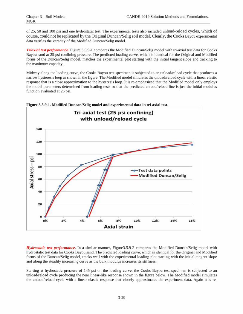
Chapter 3 – Soil Models CANDE-2019 Solution Methods and Formulations. MGK
3-29
of 25, 50 and 100 psi and one hydrostatic test. The experimental tests also included unload-reload cycles, which of course, could not be replicated by the Original Duncan/Selig soil model. Clearly, the Cooks Bayou experimental data verifies the veracity of the Modified Duncan/Selig model. Triaxial test performance. Figure 3.5.9-1 compares the Modified Duncan/Selig model with tri-axial test data for Cooks Bayou sand at 25 psi confining pressure. The predicted loading curve, which is identical for the Original and Modified forms of the Duncan/Selig model, matches the experimental plot starting with the initial tangent slope and tracking to the maximum capacity. Midway along the loading curve, the Cooks Bayou test specimen is subjected to an unload/reload cycle that produces a narrow hysteresis loop as shown in the figure. The Modified model simulates the unload/reload cycle with a linear elastic response that is a close approximation to the hysteresis loop. It is re-emphasized that the Modified model only employs the model parameters determined from loading tests so that the predicted unload/reload line is just the initial modulus function evaluated at 25 psi. Figure 3.5.9-1. Modified Duncan/Selig model and experimental data in tri-axial test.
Hydrostatic test performance. In a similar manner, Figure3.5.9-2 compares the Modified Duncan/Selig model with hydrostatic test data for Cooks Bayou sand. The predicted loading curve, which is identical for the Original and Modified forms of the Duncan/Selig model, tracks well with the experimental loading plot starting with the initial tangent slope and along the steadily increasing curve as the bulk modulus increases its stiffness. Starting at hydrostatic pressure of 145 psi on the loading curve, the Cooks Bayou test specimen is subjected to an unload/reload cycle producing the near linear-like response shown in the figure below. The Modified model simulates the unload/reload cycle with a linear elastic response that closely approximates the experiment data. Again it is re-

Chapter 3 – Soil Models CANDE-2019 Solution Methods and Formulations. MGK
3-30
emphasized that the Modified model only employs the model parameters determined from loading tests wherein the predicted unload/reload linear slope is equal to the slope of the loading curve at the point of departure/return. Figure 3.5.9-2. Modified Duncan/Selig model and experimental data in hydrostatic test.
Additional examples on the performance of Katona’s modified Duncan/Selig soil model are provided in Reference 29 wherein it is shown that the Modified model provides a realistic approach to simulate compaction loading on soil layers without using the artificial squeeze layer technique.

Chapter 3 – Soil Models CANDE-2019 Solution Methods and Formulations. MGK
3-31
3.6 Extended Hardin Soil Model The extended Hardin soil model is a variable-modulus elasticity formulation using stress/strain-dependent functions for the shear modulus and Poisson ratio. Basically, the model exhibits stiffening of constitutive moduli when confining stress increases and softening when shear strain increases. Hardin’s original work for the variable shear modulus formulation, which is based on a hyperbolic relationship between shear stress and shear strain, is summarized in a 1973 Air Force technical report (Reference 22). In 1974 a variable Poisson ratio function was developed to be the companion elasticity function so that together the two elasticity functions, shear modulus and Poisson ratio, are referred to as the extended Hardin soil model. Reference 1 documents the development of the variable Poisson function as well as validation of the shear modulus function against an independent set of experimental data. In many ways the extended Hardin model is similar in behavior to the Duncan and Duncan/Selig models, although the later models are more popular and are supported by a larger database of soil parameters dependent on soil quality and compaction. However, a unique feature of the extended Hardin model is that the soil parameters for the shear modulus function are characterized in terms fundamental soil properties including void ratio, plasticity index and percent saturation of the soil. From an overall perspective, the extended Hardin soil model functions are used to define the nonlinear components of an isotropic, elasticity-based constitutive matrix for plane-strain conditions as expressed below.
x 11 12 x
y 12 11 y
33
Δσ C C 0 ΔεΔσ = C C 0 ΔεΔτ 0 0 C Δγ
Equation 3.6-1
where, x yΔσ , Δσ , Δτ = stress increments for x-direction, y-direction and shear components, respectively
x yΔε , Δε , Δγ = strain increments for x-direction, y-direction and shear components, respectively
11 12 33C , C , C = nonlinear coefficients dependent on shear modulus and Poisson ratio functions. The table below shows the relationship between the constitutive matrix components and the shear modulus and Poisson ratio functions that define the extended Hardin model. Table 3.6.1-1 Components for constitutive matrix relationship to moduli functions
Components of Constitutive matrix
G = shear modulus
ν = Poisson ratio (G, ν)
G = shear modulus B = bulk modulus
(G, B)
C11 =
2G(1- ν)
1- 2ν
4B + G 3
C12 =
2G ν1- 2ν
2B - G 3
C33 =
G
G
The middle column in the above table defines the matrix coefficients C11, C12 and C13 in terms of shear modulus and Poisson ratio, which are the elastic parameter functions directly developed for the extended Hardin soil model. The third column defines the matrix coefficients in terms of shear modulus and bulk modulus, which is a more natural pair of

Chapter 3 – Soil Models CANDE-2019 Solution Methods and Formulations. MGK
3-32
elasticity functions and often easier to implement. The equivalence between column 2 and 3 is given by the elasticity relationship,
2(1+ ν)B = G3(1- 2ν)
Equation 3.6-2
The motivation for choosing Poisson ratio as second elasticity function is because it easy to develop a smooth function that insures Poisson ratio remains within the admissible bounds, 0 ≤ υ ≤ ½. In contrast, the constraints on an independent bulk modulus function requires that B > 2/3 G, which is more difficult to achieve with a smooth function.
3.6.1 Hardin shear modulus development Hardin’s formulation is based on experimental observations of soil behavior from standard tri-axial tests. A standard tri-axial test is conducted by placing a cylindrical soil specimen in a pressure chamber and initially subjecting the specimen to a uniform hydrostatic pressure, called σ3. Next a steadily increasing axial load is applied to the specimen producing a net axial stress, called σ1, which includes the hydrostatic pressure. Note that σ3 and σ1 are principal stresses in the lateral and axial directions, respectively. The difference in principal stresses σ1 – σ3 is equal to twice the maximum shear stress occurring on 45-degree plane. As the axial stress increases, axial strain ε1 is computed by measuring the axial shortening of the specimen divided by the specimen length. Similarly, the lateral strain ε3 is measured at each load step so that the maximum shear stain is equal to ε1 - ε3. Note that ε1 and ε3 do not include the initial hydrostatic strain and the algebraic signs must be strictly observed in computing differences. The above concepts are summarized below.
1 31τ = (σ - σ )2
Equation 3.6-3
1 3γ = ε - ε Equation 3.6-4 sτ = G γ (implied nonlinear relationship) Equation 3.6-5 where, τ = accumulated shear stress from tri-axial test
γ = accumulated shear strain from tri-axial test
sG = secant shear modulus, a function of stress and strain The curve in Figure 3.6.2-1 is an idealized plot of shear stress versus shear strain for a typical tri-axial test. Here, Gmax is the initial slope at zero shear strain and τmax is the maximum shear strain at failure. As discussed subsequently, Gmax and τmax are dependent on the hydrostatic stress level.

Chapter 3 – Soil Models CANDE-2019 Solution Methods and Formulations. MGK
3-33
Figure 3.6.2-1 Idealized shear stress-strain curve for tri-axial test
Hardin hyperbolic function. Hardin’s fundamental insight is that for any tri-axial test, the shear stress-strain curve is fairly well approximated by equating the shear stress to a hyperbolic function of shear strain as follows,
max
h
Gτ = γ1+ γ
Equation 3.6-6
h0.4r
r
γ αγ = 1 + γγ exp( )γ
( ) Equation 3.6-7
r max 1γ = G /C Equation 3.6-8 where, maxG = initial slope for shear modulus (dependent on hydrostatic stress)
hγ = hyperbolic strain function
rγ = reference shear stain α = dimensionless soil parameter, related to soil type and percent saturation.
1C = soil parameter with units of stress, related to void ratio, percent saturation, and plasticity index. As shear strain increases to infinity, the shear stress in Equation 3.6-6 approaches an asymptotic limit representing the maximum shear stress (or shear failure stress) given by, max max rτ = G γ Equation 3.6-9

Chapter 3 – Soil Models CANDE-2019 Solution Methods and Formulations. MGK
3-34
Initial shear modulus. Based on a wide variety of soil tests as typified by the above figure, Hardin discovered that the initial shear modulus increased in proportion with the square root of the initial tri-axial confining pressure as expressed below.
max 1 mG = S σ Equation 3.6-10
where, maxG = initial shear modulus when shear strain = 0
1S = soil parameter related to void ratio (units in psi )
m 11 22 33σ = 1/3(σ + σ + σ ) = hydrostatic stress (psi) Equations 3.6-6 through 3.6-10 form the complete mathematical description of the Hardin secant shear modulus function, which is characterized by three soil model parameters, C1 , S1 and α. The direct method of determining the soil model parameters is to conduct a series of tri-axial tests on the particular soil being investigated. Alternatively, Hardin has developed an indirect method for determining soil parameters based on fundamental soil properties. Both the direct and indirect methods are presented below. Direct method of soil parameter identification. Clearly the most accurate way to determine the shear modulus parameters, C1 , S1 and α, is to perform a series of tri-axial tests on the soil under investigation. For each confining pressure σ3, it is required to plot an experimental stress-strain curve similar to Figure 3.6.2-1 and then follow the steps below.
1. Construct the initial tangent at zero shear stain and denote its value as Gmax. Based in Equation 3.6-10, the parameter S1 may be computed as follows.
1 max 3S = G / σ Equation 3.6-11
Ideally each confining pressure would produce the same value for S1. However since the model is not perfect, the final value for S1 should be the average value determined from all initial confining pressures.
2. Using the measured value of Gmax from step 1 along with the experimentally observed max shear stress τmax ,
the parameter C1 may be computed by combining Equations 3.6-8 and 3.6-9 as follows.
21 max maxC = G /τ Equation 3.6-12
In an ideal world, the computed value of C1 should be the same for all confining pressures. However since the model is not perfect, the final value for C1 should be the average value determined from all initial confining pressures.
3. The third and last soil parameter α controls the shape (concavity )of the shear stress-strain curve in Figure 3.6.2-1. Since all parameters of the secant shear modulus model are known except α, Equation 3.6-6 may be applied at a single experimental data point (τ*, γ*) to provide an algebraic equation to solve for α. A natural data point to select is midway in the stress range, τ* = ½ τmax along with the corresponding experimentally measured shear strain γ*.
Indirect method of soil parameter identification. A particularly useful result of Hardin’s work is that he developed an indirect method for determining soil parameters based on fundamental soil properties. This was accomplished by correlating the results of many tri-axial tests for many types soil with basic soil properties including void ratio, percent saturation, and plasticity index.

Chapter 3 – Soil Models CANDE-2019 Solution Methods and Formulations. MGK
3-35
Listed below are the expressions he developed to quantify the soil parameters C1 , S1 and α for three broad classes of soil, granular, mixed and cohesive.
2 2
1 0.6F RC =
0.6 - 0.25(PI) (units psi) Equation 3.6-13
1S = 1230 F (units psi ) Equation 3.6-14
3.2 for granular soil2.54(1+0.02S) for mixed soil1.12(1+0.02S) for cohesive soil
α =
(dimensionless) Equation 3.6-15
where, 2
for all soil types(2.973 - e)F =
1 + e
1100 for granular soil1100 - 6.0 S for mixed and cohesive soil
R=
and, e = void ratio (0 ≤ e ≤ 1)
S = percent saturation (0 ≤ S ≤ 100) PI = plasticity index (0 ≤ PI ≤ 1)
Thus knowing the type of soil, void ratio, percent saturation, and plasticity index, Hardin’s secant shear modulus function is completely characterized without the need of a tri-axial test.
3.6.2 Poisson ratio development Poisson ratio may be back calculated from tri-axial test data providing that principal stresses and principal strains are measured during the test. Reference 1 presents a study showing back-calculated values of Poisson ratio for a sequence of tri-axial tests with increasing confining pressure. Two significant findings from this study are summarized below.
1. For each individual tri-axial test with a specified confining pressure, the measured Poisson ratio increases as shear strain increases. Starting at a low value of approximately 0.01, the measured Poisson ratio asymptotically approaches an upper limit, nominally equal to 0.49, as the shear strain approaches the shear failure limit.
2. When confining pressure is increased, the starting and ending values of Poisson ratio remain the same as noted
above, however the rate of increase of Poisson ratio with shear strain increases as confining pressure increases. Said another way, the measured value of Poisson ratio at a given level of shear strain is inversely related to the confining pressure. The above two observations are illustrated in Figure 3.6.3-1.

Chapter 3 – Soil Models CANDE-2019 Solution Methods and Formulations. MGK
3-36
Figure 3.6.3-1 Illustration of measured Poisson ratio from tri-axial tests.
Poisson ratio function. A Poisson ratio function that simulates the above two observations is shown below, wherein γp is a scaled measure of shear stain.
min p max
p
ν + γ νν =
1 + γ Equation 3.6-16
pr
qγ = γγ
Equation 3.6-17
where, ν = Poisson ratio function. pγ = scaled shear strain measure.
rγ = Hardin reference shear strain (= Gmax/C1 from Equation 3.6-8) and, minν = Poisson function parameter denoting minimum value (dimensionless constant)
maxν = Poisson function parameter denoting maximum value (dimensionless constant) q = Poisson function parameter controlling curve shape (dimensionless constant) Upon inspecting the Poisson ratio function, it is clear that when shear strain is zero, ν = νmin, and when shear strain becomes very large, ν = νmax. Thus, the Poisson ratio function satisfies the first observation noted above. The second

Chapter 3 – Soil Models CANDE-2019 Solution Methods and Formulations. MGK
3-37
observation is achieved by defining γp with Hardin reference strain γr in the denominator as shown in Equation 3.16-7. Since γr is proportional to Gmax and Gmax is an increasing function of confining pressure, γp is reduced for tests with higher confining pressures so that the Poisson ratio function behaves as illustrated in the above. It is important to realize that the predicted and observed variation in Poisson ratio as portrayed in Figure 3.6.3-1 is only for the case of a standard tri-axial loading environment. When Equation 3.6-16 is used to predict the behavior of Poisson ratio in a uniaxial-strain loading environment (K0-test), the Poisson ratio prediction remains nearly constant as axial strain (or shear strain) increases. This is because the steadily increasing confining pressure increases the value of Gmax at nearly the same rate as the increase in strain so that γp remains nearly constant in accordance with observed behavior. Parameter identification. The Poisson ratio function requires identifying values for three model parameters, νmin, νmax and q. The study presented in Reference 1 measured Poisson ratio values from five tri-axial tests with confining pressures ranging from 25 psi to 250 psi. The soil specimens were dry, dense sand, and the model parameters identified as, minν = 0.10
maxν = 0.49 q = 0.26 Choosing values for νmin and νmax are straightforward observations from the experimental data, and the selection of the shape parameter q is determined by standard curve fitting techniques. The study concludes that the Poisson ratio function with the above parameter values is in excellent agreement with the measured Poisson ratio data points for all five tri-axial tests. Of course, it is always best to conduct tri-axial tests on new soils to identify the parameters of the Poisson ratio function. However, experience has shown that νmin, νmax and q are not overly sensitive to the type of soil and soil properties, thus if no other data is available the above parametric values are fairly reasonable for all soil types.
3.6.3 Summary of extended Hardin soil model functions The extended Hardin soil model is composed of the secant shear modulus function and the Poisson ratio function both of which are functions of maximum shear strain and hydrostatic pressure. The secant shear modulus function is given by the following function and sub functions.
maxs
h
GG = 1+ γ
= shear modulus function Equation 3.6-18
h0.4r
r
γ αγ = 1 + γγ exp( )γ
( ) = hyperbolic strain function Equation 3.6-19
r max 1γ = G /C = reference shear stain Equation 3.6-20
max 1 mG = S σ = initial shear modulus when shear strain = 0 Equation 3.6-21
where, γ = maximum shear strain
m 11 22 33σ = 1/3(σ + σ + σ ) = hydrostatic stress (units psi) and, 1S = soil parameter related to void ratio (units in psi )
α = soil parameter, related to soil type and percent saturation (dimensionless) 1C = soil parameter related to void ratio, percent saturation, and plasticity index (units psi)

Chapter 3 – Soil Models CANDE-2019 Solution Methods and Formulations. MGK
3-38
Parameter identification for C1 , S1 and α may be accomplished directly with tri-axial tests as outlined in the discussion associated with Equations 3.6-11 and 3.6-12. Alternatively the parameters may be quantified by the indirect method outlined with the discussion associated with Equations 3.6-13, -14, and –15. The Poisson ratio function is given by the following function and sub functions.
min p max
p
ν + γ νν =
1 + γ = Poisson ratio function Equation 3.6-22
pr
qγ = γγ
= scaled shear strain measure Equation 3.6-23
where, rγ = Hardin reference shear strain (= Gmax/C1 from Equation 3.6-20) and, minν = Poisson function parameter denoting minimum value (dimensionless constant)
maxν = Poisson function parameter denoting maximum value (dimensionless constant) q = Poisson function parameter controlling curve shape (dimensionless constant)
Parameter identification for νmin, νmax and q may be accomplished with tri-axial tests as outlined in the discussion in Section 3.6.3. If no independent test data is available, the default values, νmin, = 0.1, νmax = 0.49, and q = 0.26 are reasonable for all soil types. The overall behavior of the extended Hardin soil model mimics the actual behavior of soil. The model exhibits a stiffening behavior when confining pressure dominates shear strain, and conversely a softening behavior when shear strain dominates confining pressure. Lastly, it is emphasized the extended Hardin soil model is a nonlinear elasticity model and behaves the same in loading or unloading. Like the Duncan and Duncan/Selig soil models, additional research needs to be done in order to incorporate plasticity-like concepts into the model so that unloading behavior can be simulated without violating energy theorems and continuity principles.
3.6.4 Implementation of Harden model and nonlinear solution strategy To implement the extended Hardin model into the plane-strain constitutive matrix given by Equation 3.6-1, it is more convenient to use the bulk modulus function with the shear modulus function (G, B) rather than the Poisson ratio function (G ,ν) as was indicated in Table 3.6.1-1. The bulk modulus function is related to the extended Hardin functions by elasticity identity relationships as,
s s2(1+ ν)B = G3(1- 2ν)
Equation 3.6-24
where, sB = secant bulk modulus function
sG = secant shear modulus function (Equation 3.6-18) ν = Poisson ratio function (Equation 3.6-22) Letting σ1, σ2, σ3 be the total principal stresses and ε1, ε2 and ε3 the corresponding total principal stains, then, the secant moduli (Gs, Bs) relate total stress quantities to total strain quantities as follows.

Chapter 3 – Soil Models CANDE-2019 Solution Methods and Formulations. MGK
3-39
sτ = G γ Equation 3.6-25
m sσ = B φ Equation 3.6-26 where, 1 3τ = (σ -σ )/2 = maximum shear stress
1 3γ = ε - ε = maximum shear strain
m 1 2 3σ = (σ + σ + σ )/3 = mean stress or hydrostatic stress
1 2 3φ = ε + ε + ε = volumetric strain Chord moduli representation. To progress from load step i to load step i+1, the moduli must be expressed as incremental chord moduli, which are related to secant moduli as illustrated in the figures below. Figure 3.6.5-1 Chord modulus relationship to secant modulus for shear modulus.

Chapter 3 – Soil Models CANDE-2019 Solution Methods and Formulations. MGK
3-40
Figure 3.6.5-2 Chord modulus relationship to secant modulus for bulk modulus.
The incremental relationships between load steps i and i+1 as portrayed in the above figures are defined below. cΔτ = G Δγ Equation 3.6-27
m cΔσ = B Δφ Equation 3.6-28
( )s i+1 ii+1c
i+1 i
G γ - τG =
γ - γ Equation 3.6-29
( )s i+1 m(i)i+1c
i+1 i
B φ - σB =
φ - φ Equation 3.6-30
where, cG = chord shear modulus from load step i to i+1
cB = chord bulk modulus from load step i to i+1
i+1 iΔτ = τ - τ = shear stress increment
i+1 iΔγ = γ - γ = shear strain increment
m m(i+1) miΔσ = σ - σ = mean stress increment
i+1 iΔφ = φ - φ = volumetric strain increment.

Chapter 3 – Soil Models CANDE-2019 Solution Methods and Formulations. MGK
3-41
Nonlinear solution strategy. The solution strategy is based on a direct iterative approach, also called trial and error. We begin with the understanding that we have a converged solution at load step i so that we know the total stress and total strain state, σ i and ε i , respectively. Our objective is to advance the solution to load step i+1 following the steps below.
(1) To obtain the first trial solution, assume the values for Gc and Bc remain the same as they were for load step i for each individual element.
(2) Construct the element stiffness matrix using Gc and Bc to define the current constitutive matrix for each
element (Equation 3.6-1)
(3) Assemble the global stiffness matrix and load increment vector for step i+1. Solve the system for a trial solution and recover current estimates for increments of stress and strain vectors. Update trial vectors for total stress and strain as indicated below.
Δε = incremental strain vector determined from strain-displacement relationship.
Δσ = incremental stress vector determined from current constitutive matrix i+1 iε = ε + Δε
i+1 iσ = σ + Δσ (4) Based on the known stress-strain state at step i and the estimated stress-strain state at step i+1, compute new
estimates for Gc and Bc .
( )s i+1 ii+1c
i+1 i
G γ - τG =
γ - γ (see Equation 3.6-18)
( )s i+1 m(i)i+1c
i+1 i
B φ - σB =
φ - φ (see Equations 3.6-18, -22, -24)
(5) If Gc and Bc computed in step 4 are sufficiently close to the previous estimates, say within 1% difference, then
the load step has converged, the solution is saved, and control shifts back to step 1 to advance to the next load step. Otherwise, the iterative process continues wherein the incremental solution is discarded and control shifts back to step 2 to repeat the load increment using the new values for Gc and Bc to get a new trial solution.
Typically the above algorithm converges for all elements in three to ten iterations for each load step, depending on the scope of the problem. Convergence means that static equilibrium and the constitutive matrix are simultaneously satisfied.

Chapter 3 – Soil Models CANDE-2019 Solution Methods and Formulations. MGK
3-42
3.7 Mohr/Coulomb Plasticity Model with Tension Cutoff
3.7.1 Pros and Cons of Mohr/Coulomb Model The classical Mohr/Coulomb elastic-perfectly plastic constitutive model is often used by geotechnical engineers to simulate soil shear-failure when analyzing soil-structure systems such as in-situ soil beneath footings and walls. The use of this classical model is supported by popular commercial finite programs such as ABAQUS, NASTRAN and FLAX3D, which recommend the use of the Mohr/Coulomb elastic-perfectly plastic model for soil-structure analysis. An inherent attribute of the plasticity formulation is that it includes permanent deformation when unloading from the plastic domain as opposed to nonlinear elasticity models that retrace the same load/unload path. In spite of these attributes, the classical Mohr/Coulomb plasticity model is less than ideal because it predicts shear failure to occur as an abrupt, rather than a gradual, phenomena as observed in most soils used for backfill. Another shortcoming is that the model does not exhibit increasing stiffness with increased confining pressure as generally observed in soils. In contrast, the Duncan/Selig soil model captures the entire suite of observed soil behavior for all loading environments. Moreover, the Katona modified form of the Duncan/Selig model also captures the linear-like unload/reload response of soils similar to plasticity models. For the record, the finite element program PLAXIS offers a sophisticated plasticity-based hardening model whose hardening rule was developed to mimic the Duncan/Selig variable-modulus model under loading conditions (Reference 30). Accordingly, the Modified Duncan/Selig model and the PLAXIS hardening soil model are judged equivalent for loading and unloading environments and are well suited for modeling the backfill soil around culverts. Irrespective of the limitations of the classical Mohr/Coulomb model to simulate the full range of soil behavior, this section is devoted to the development of the Mohr/Coulomb model and its implementation in the CANDE-2019 program. Although it is generally recommended to use the Duncan/Selig model to represent fill-soil behavior, the motivation for developing and offering the classical Mohr/Coulomb constitutive model is threefold:
1. Some in-situ soils such as stiff clays are well represented by the Mohr/Coulomb model. 2. Since some finite element programs are limited to the classical Mohr/Coulomb plasticity soil model, it
is convenient to include the model in CANDE in order to make direct comparisons. 3. Materials other than soils, such as metals, are well represented by the Tresca form of the
Mohr/Coulomb model (ϕ = 0). With the above understanding, the Mohr/Coulomb plasticity model as offered in CANDE is developed in the following paragraphs. The last section provides a comparison of the performance of the Mohr/Coulomb and the Duncan/Selig soil models with experimental data for Cooks Bayou sand in tri-axial, hydrostatic and confined compression loading environments.
3.7.2 Basic Plasticity Concepts From a one-dimensional view point the Mohr-Coulomb model may be viewed as an elastic spring in series with a plastic slider that is abruptly activated when the shear stress exceeds a stress dependent limit as depicted in Figure 3.7.1-1 below.
Figure 3.7.2-1. One dimensional analogue of Mohr/Coulomb elastic-plastic model
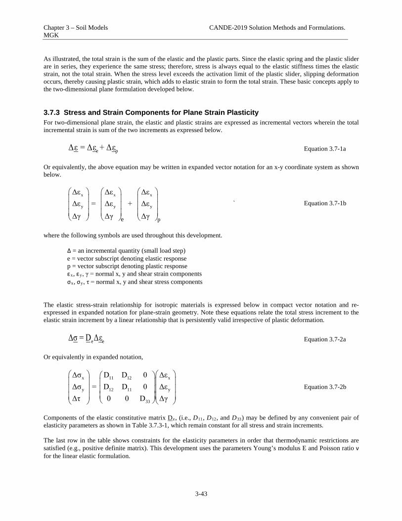
Chapter 3 – Soil Models CANDE-2019 Solution Methods and Formulations. MGK
3-43
As illustrated, the total strain is the sum of the elastic and the plastic parts. Since the elastic spring and the plastic slider are in series, they experience the same stress; therefore, stress is always equal to the elastic stiffness times the elastic strain, not the total strain. When the stress level exceeds the activation limit of the plastic slider, slipping deformation occurs, thereby causing plastic strain, which adds to elastic strain to form the total strain. These basic concepts apply to the two-dimensional plane formulation developed below.
3.7.3 Stress and Strain Components for Plane Strain Plasticity For two-dimensional plane strain, the elastic and plastic strains are expressed as incremental vectors wherein the total incremental strain is sum of the two increments as expressed below.
e pΔε = Δε + Δε Equation 3.7-1a Or equivalently, the above equation may be written in expanded vector notation for an x-y coordinate system as shown below.
x x x
y y y
pe
Δε Δε ΔεΔε = Δε + ΔεΔγ Δγ Δγ
` Equation 3.7-1b
where the following symbols are used throughout this development. Δ = an incremental quantity (small load step) e = vector subscript denoting elastic response p = vector subscript denoting plastic response εx, εy, γ = normal x, y and shear strain components σx, σy, τ = normal x, y and shear stress components The elastic stress-strain relationship for isotropic materials is expressed below in compact vector notation and re-expressed in expanded notation for plane-strain geometry. Note these equations relate the total stress increment to the elastic strain increment by a linear relationship that is persistently valid irrespective of plastic deformation.
e eΔσ = D Δε Equation 3.7-2a Or equivalently in expanded notation,
x 11 12 x
y 12 11 y
33
Δσ D D 0 ΔεΔσ = D D 0 ΔεΔτ 0 0 D Δγ
Equation 3.7-2b
Components of the elastic constitutive matrix De, (i.e., D11, D12, and D33) may be defined by any convenient pair of elasticity parameters as shown in Table 3.7.3-1, which remain constant for all stress and strain increments. The last row in the table shows constraints for the elasticity parameters in order that thermodynamic restrictions are satisfied (e.g., positive definite matrix). This development uses the parameters Young’s modulus E and Poisson ratio ν for the linear elastic formulation.

Chapter 3 – Soil Models CANDE-2019 Solution Methods and Formulations. MGK
3-44
TABLE 3.7.3-1. Popular pairs of elastic parameters for constitutive matrix.
Elastic matrix component
M = Confined mod. K0 = Lateral coeff.
E = Young’s mod ν = Poisson ratio
B = Bulk mod. G = Shear mod.
E = Young’s mod. B = Bulk mod.
D11 = M E(1- ν)/(1+ ν)(1-2 ν) B + (4/3)G B(9B+3E)/(9B-E) D12 = M K0 Eν/(1+ ν)(1-2 ν) B – (2/3)G 3B(3B-E)/(9B-E)
D33 = (D11- D12)/2 =
M(1-K0)/2 E/2(1+ ν) G 3EB/(9B-E)
Constraints M > 0 0 ≤ K0 ≤ 1
E > 0 0 ≤ ν ≤ 1/2
B > 0 0 ≤ G ≤ (3/2)B
E > 0 E/3 ≤ B < ∞
3.7.4 Plastic failure surface of Mohr/Coulomb Model The classical Mohr/Coulomb formulation employs a non-hardening yield surface equivalently called the failure surface. Like the Tresca failure criterion that is defined by a maximum shear stress “c”, the Mohr/Coulomb failure surface is also a shear based failure criterion; however, shear strength increases linearly with the compressive normal stress acting on the failure plane. This concept is like the theory of Coulomb friction, which linearly increases sliding resistance in proportion to the compressive normal force. The Mohr-Coulomb shear strength equation is shown below and depicted in Figure 3.7.4-1. Note that the development follows the standard sign convention wherein positive normal stresses are in tension and negative stresses are in compression.
max tannCτ σ φ= − Equation 3.7-3 where, τmax = absolute maximum achievable shear stress C = cohesion of material (stress units, user defined) ϕ = angle of internal friction (radians, user defined) σn = normal stress on plane of failure (negative stress is compressive) Tcut = Tension cutoff (tensile stress, user defined)
Figure 3.7.4-1 Mohr/Coulomb failure surface in (σn, τ) stress space.
Failure Surface
Shear Stress τ
Normal stress σn
C φ
τmax = C - σntanφ .(σn,τ)
. Ccotϕ
Tcut

Chapter 3 – Soil Models CANDE-2019 Solution Methods and Formulations. MGK
3-45
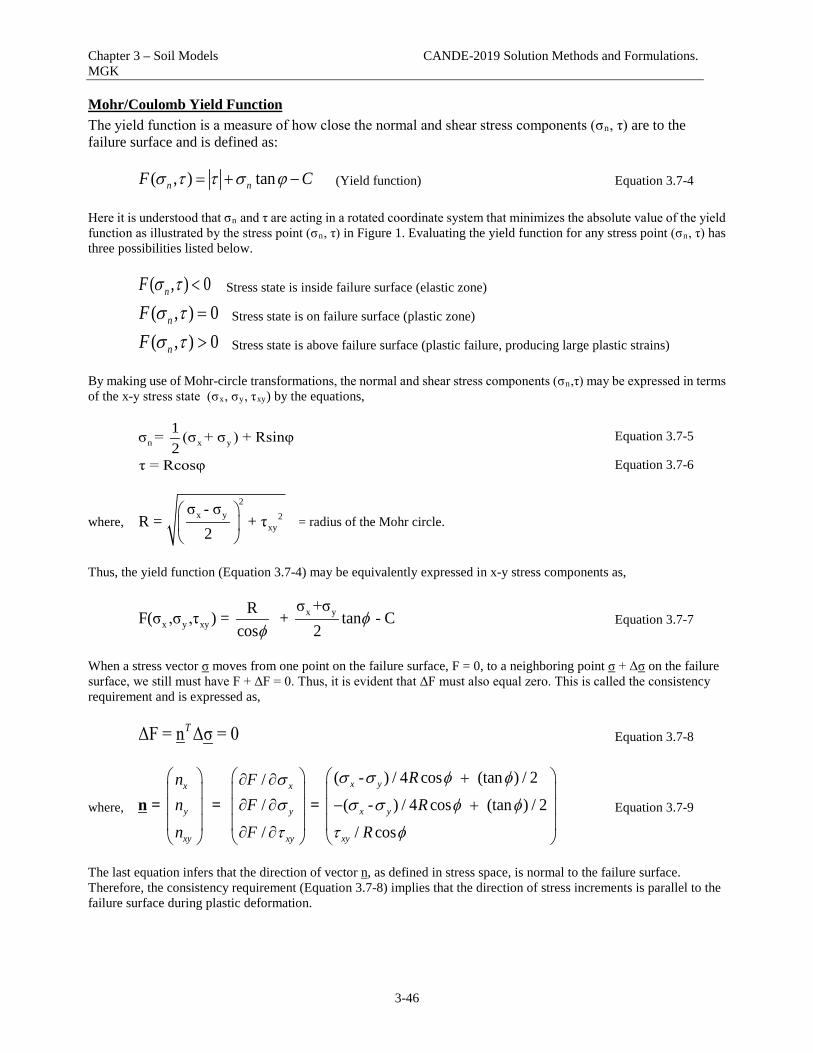
Chapter 3 – Soil Models CANDE-2019 Solution Methods and Formulations. MGK
3-46
Mohr/Coulomb Yield Function The yield function is a measure of how close the normal and shear stress components (σn, τ) are to the failure surface and is defined as:
( , ) tann nF Cσ τ τ σ ϕ= + − (Yield function) Equation 3.7-4 Here it is understood that σn and τ are acting in a rotated coordinate system that minimizes the absolute value of the yield function as illustrated by the stress point (σn, τ) in Figure 1. Evaluating the yield function for any stress point (σn, τ) has three possibilities listed below.
( , ) 0nF σ τ < Stress state is inside failure surface (elastic zone)
( , ) 0nF σ τ = Stress state is on failure surface (plastic zone)
( , ) 0nF σ τ > Stress state is above failure surface (plastic failure, producing large plastic strains) By making use of Mohr-circle transformations, the normal and shear stress components (σn,τ) may be expressed in terms of the x-y stress state (σx, σy, τxy) by the equations,
n x y1σ = (σ + σ ) + Rsinφ 2
Equation 3.7-5
τ = Rcosφ Equation 3.7-6
where, 2
x y 2xy
σ - σR = + τ
2
= radius of the Mohr circle.
Thus, the yield function (Equation 3.7-4) may be equivalently expressed in x-y stress components as,
xy
yx xy
σ +σRF( ) = + tan - Ccos 2
σ ,σ ,τ φφ
Equation 3.7-7
When a stress vector σ moves from one point on the failure surface, F = 0, to a neighboring point σ + Δσ on the failure surface, we still must have F + ΔF = 0. Thus, it is evident that ΔF must also equal zero. This is called the consistency requirement and is expressed as,
ΔF = n Δσ = 0T Equation 3.7-8
where,
( - ) / 4 cos (tan ) / 2// ( - ) / 4 cos (tan ) / 2/ / cos
x yx x
y y x y
xy xy xy
Rn Fn F Rn F R
σ σ φ φσσ σ σ φ φ
τ τ φ
+∂ ∂
∂ ∂ − + ∂ ∂
n = = = Equation 3.7-9
The last equation infers that the direction of vector n, as defined in stress space, is normal to the failure surface. Therefore, the consistency requirement (Equation 3.7-8) implies that the direction of stress increments is parallel to the failure surface during plastic deformation.

Chapter 3 – Soil Models CANDE-2019 Solution Methods and Formulations. MGK
3-47
Principal Stress Space. The forgoing development applies to a general stress-state σx, σy, τxy in any x-y coordinate system. To gain visual insight, it is useful to consider the case of principal stresses wherein σx = σ1, σy = σ2, and τxy = 0. For a stress state expressed in principal stress, the normal components to the yield surface are not dependent on stress magnitudes but only on the signs of the principal stresses as shown below.
1 1 2
2 1 2
( - ) / 2cos (tan ) / 2( - ) / 2cos (tan ) / 2
0xy
n signn signn
σ σ ϕ ϕσ σ ϕ ϕ
+ − +
n = =
In principal stress space, the Mohr-Coulomb failure surface is wedge shaped as shown in the figure below by the red lines, which are symmetric about the hydrostatic path σ1 = σ2. Also shown are the normal vectors in principal stress space, one for the upper surface and one for the lower surface. Figure 3.7.6-1. Mohr-Coulomb failure surfaces in principal stress space.
The Mohr-Coulomb failure surface in principal stress space will be used to throughout this writing to illustrate the zones of elasticity, plasticity and tension cutoff.
(cotφC, cotφC)
(0, 2cosφC/(1+sinφ))
σ1 compression
negative
σ2 compression
negative
1 2 1Lower Failure Surface (σ > σ , σ less negative)
1 2(1+ sinφ) (1- sinφ)σ - σ - C = 0(2cosφ) (2cosφ)
2 1 2Upper Failure Surface (σ > σ , σ less negative)
1 2+ -(1 - sinφ) (1 + sinφ)
- σ σ C = 0(2cosφ) (2cosφ)
(-2cosφC/(1-sinφ), 0)
(0, -2cosφC/(1-sinφ))
n
n
..
. . (2cosφC/(1+sinφ), 0)
.
σ1 = σ2
σ1 +
σ2 +
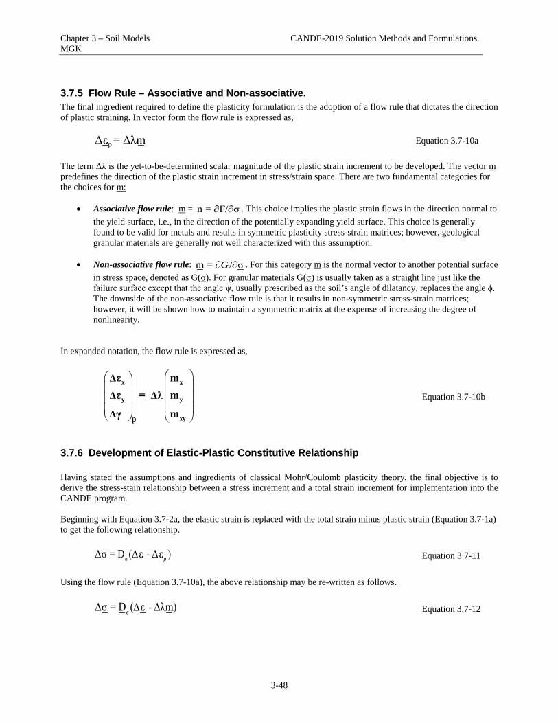
Chapter 3 – Soil Models CANDE-2019 Solution Methods and Formulations. MGK
3-48
3.7.5 Flow Rule – Associative and Non-associative. The final ingredient required to define the plasticity formulation is the adoption of a flow rule that dictates the direction of plastic straining. In vector form the flow rule is expressed as,
pΔε = Δλm Equation 3.7-10a
The term Δλ is the yet-to-be-determined scalar magnitude of the plastic strain increment to be developed. The vector m predefines the direction of the plastic strain increment in stress/strain space. There are two fundamental categories for the choices for m:
• Associative flow rule: m = n = F/ σ∂ ∂ . This choice implies the plastic strain flows in the direction normal to the yield surface, i.e., in the direction of the potentially expanding yield surface. This choice is generally found to be valid for metals and results in symmetric plasticity stress-strain matrices; however, geological granular materials are generally not well characterized with this assumption.
• Non-associative flow rule: m = / σG∂ ∂ . For this category m is the normal vector to another potential surface
in stress space, denoted as G(σ). For granular materials G(σ) is usually taken as a straight line just like the failure surface except that the angle ψ, usually prescribed as the soil’s angle of dilatancy, replaces the angle ϕ. The downside of the non-associative flow rule is that it results in non-symmetric stress-strain matrices; however, it will be shown how to maintain a symmetric matrix at the expense of increasing the degree of nonlinearity.
In expanded notation, the flow rule is expressed as,
x x
y y
xyp
Δε mΔε = Δλ mΔγ m
Equation 3.7-10b
3.7.6 Development of Elastic-Plastic Constitutive Relationship Having stated the assumptions and ingredients of classical Mohr/Coulomb plasticity theory, the final objective is to derive the stress-stain relationship between a stress increment and a total strain increment for implementation into the CANDE program. Beginning with Equation 3.7-2a, the elastic strain is replaced with the total strain minus plastic strain (Equation 3.7-1a) to get the following relationship.
eΔσ = D (Δε - Δε )p Equation 3.7-11
Using the flow rule (Equation 3.7-10a), the above relationship may be re-written as follows.
σ = D ( ε - λm)e∆ ∆ ∆ Equation 3.7-12

Chapter 3 – Soil Models CANDE-2019 Solution Methods and Formulations. MGK
3-49
In order to determine the scalar Δλ, the consistency requirement demands that the scalar product nTΔσ = 0 when plastic deformation occurs. Thus performing the dot product on Equation 3.7-12 and rearranging terms, Δλ is determined in terms of the total strain increment as shown below.
T
T
n D ελ = n D m
e
e
∆∆ Equation 3.7-13
Again returning to Equation 3.7-12 with above value of Δλ, we obtain the desired general stress-strain relationship shown below,
pσ = (D - D ) εe∆ ∆ Equation 3.7-14 wherein Dp is the plasticity matrix given by,
Tp
1D = ( ) D n D α
me e Equation 3.7-15
and, alpha is a scalar given by, T
eα = n D m . As described by Equation 3.7-15, Dp is a non-symmetric matrix because mnT is not symmetric unless an associative flow is assumed where m = n. There is a clever trick to convert Dp into a symmetric matrix for the non-associative flow rule as follows. We begin by expressing the vector product of the plasticity matrix times the strain increment vector to get:
T Tp e e e e
1 1D ε = D mn D ε = D m (n D ε)α α
∆ ∆ ∆ Equation 3.7-16a
Note that the term in parenthesis (nTDeΔε) is a scalar quantity which can be moved as desired. Next if we multiply the above equation by unity by means of multiplying and dividing with a new scalar (mTDeΔε), then the above equation may be expressed as,
T
T Tep e e e eT
e
(n D Δε)1 κD Δε = D m (m D Δε) = D m m D Δεα (m D Δε) α
Equation 3.7-16b
Thus, the plasticity matrix with non-associative flow rule is now in a symmetric form as shown below.
Tp e eD = D mm D
ακ symmetric plasticity matrix. Equation 3.7-17
where, T
eT
e
(n D ε)κ = (m D ε)
∆∆
scalar dependent on strain increment. Equation 3.7-18
Dp is symmetric because the product mmT is a symmetric matrix as is De. The penalty for symmetry is that the scalar multiplier κ causes another level of nonlinearity because it contains the unknown strain increment. Therefore, more iterations to convergence are generally required. However, it has been shown that the time and storage efficiency of symmetric equation solvers more than makes up for additional iterations. In expanded notation, the individual components of the 3x3 plasticity matrix are shown below for the general case of a non-associative flow rule.

Chapter 3 – Soil Models CANDE-2019 Solution Methods and Formulations. MGK
3-50
211 x 12 y 11 x 12 y 12 x 11 y 11 x 12 y 33 xy
2p 12 x 11 y 11 x 12 y 12 x 11 y 12 x 11 y 33 xy
233 xy 11 x 12 y 33 xy 12 x 11 y 33 xy
(D m + D m ) (D m + D m )(D m + D m ) (D m + D m )D mD = (D m + D m )(D m + D m ) (D m + D m ) (D m + D m )D m
αD m (D m + D m ) D m (D m + D m ) (D m )
where α
κ
11 x x y y 12 x y y x 33 xy xy
x 11 x 12 y y 12 x 11 y xy 33 xy
x 11 x 12 y y 12 x 11 y xy 33 xy
= D (n m + n m ) + D (n m +n m ) + D (n m )
n (D Δε +D Δε ) + n (D Δε +D Δε ) + n (D γ ) κ =
m (D Δε +D Δε ) + m (D Δε +D Δε ) + m (D γ )
For the special case of the associative flow rule, we have m = n and κ = 1, and the plasticity matrix is given by:
211 x 12 y 11 x 12 y 12 x 11 y 11 x 12 y 33 xy
2p 12 x 11 y 11 x 12 y 12 x 11 y 12 x 11 y 33 xy
233 xy 11 x 12 y 33 xy 12 x 11 y 33 xy
(D n + D n ) (D n + D n )(D n + D n ) (D n + D n )D n1D = (D n + D n )(D n + D n ) (D n + D n ) (D n + D n )D nα
D n (D n + D n ) D n (D n + D n ) (D n )
where α
2 2 211 x y 12 x y 33 xy= D (n + n ) + 2D n n + D n
In summary, the fundamental constitutive relationship given by Equation 3.7-14 is repeated below along with a new scalar parameter β that is a multiplier of the plasticity matrix where 0 ≤ β ≤ 1.
pσ = (D - D ) εe β∆ ∆ Equation 3.7-19 The purpose of the β multiplier is to control the percentage of the plasticity matrix that is applied in any iteration of a particular load step. For example, if the starting and ending stress states remain within the elastic domain, then β =0. Conversely if the stress increment starts and remains in the plastic zone, then β = 1. As will be discussed in the subsequent section on nonlinear solution strategy, transitioning from the elastic zone to the plastic zone requires determining a fractional value of β. However, the transition from the plastic zone to the elastic zone is always done with β = 0 because this is what produces permanent plastic deformation as observed in laboratory experiments (i.e. elastic unloading).
3.7.7 Development of Tension Cutoff Methodology The Mohr-Coulomb failure surface does not mimic the complicated soil behavior that occurs when the stress state becomes predominantly tensile wherein soil particles separate and become discontinuous. To deal with this problem, a special tension cutoff methodology is introduced that simulates two important phenomena; the loss of stiffness and the inability to sustain additional tensile stress. Conversely, if the stress state changes direction and becomes compressive, then the tension cutoff model allows a gradual increase in stiffness and the ability to carry compressive stresses as the stress-state returns to the zones controlled by the Mohr-Coulomb failure surface. Tension cutoff is simulated with a plasticity-based constitutive model whose yield surface is a straight line, orthogonal to the hydrostat (σx = σy), and intersecting the hydrostat at the point σx = σy = Tcut. Specifically, the tension cutoff yield function, which is independent of shear stress, is defined by Equation 3.7-20 and illustrated in Figure 3.7.7-1.

Chapter 3 – Soil Models CANDE-2019 Solution Methods and Formulations. MGK
3-51
x y avg cutF*(σ ,σ ) = - Tσ Equation 3.7-20 where, F* = Tension cutoff yield function. σavg = ½(σx+ σy) = average (hydrostatic) stress , i.e., center of Mohr circle. Tcut = Limit of average tensile stress, a model parameter, 0 ≤ Tcut ≤ Ccotϕ Figure 3.7.7-1. Illustration of tension cutoff zone
Note that the asterisk symbol “*” is used to distinguish tension cutoff symbols from the corresponding Mohr-Coulomb symbols. Evaluation of the tension yield function for any stress state has two possible results listed below. x yF*(σ ,σ ) 0< Stress state is in Mohr-Coulomb domain - tension cutoff not activated.
x yF*(σ ,σ ) 0≥ Stress state is on or above tension cutoff surface (green) – tension plasticity activated.
σ1
σ2
Tension CutoffSpace, F* ≥ 0
M-C Failure Surface
F = R/cosφ + σavg tanφ - C
ELASTIC SPACEF < 0, F*< 0
Tcut
Tcut
Tension Cut-off
F* = σavg - T
cut
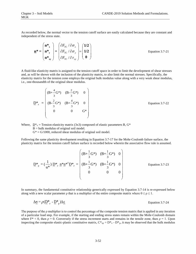
Chapter 3 – Soil Models CANDE-2019 Solution Methods and Formulations. MGK
3-52
As recorded below, the normal vector to the tension cutoff surface are easily calculated because they are constant and independent of the stress state.
///
TC x
TC y
TC xy
FFF
σσ
τ
∂ ∂ ∂ ∂ =
∂ ∂
x
y
xy
n* 1/2n* = n* = 1/2
0n* Equation 3.7-21
A fluid-like elasticity matrix is assigned to the tension cutoff space in order to limit the development of shear stresses and, as will be shown with the inclusion of the plasticity matrix, to also limit the normal stresses. Specifically, the elasticity matrix for the tension zone employs the original bulk modulus value along with a very weak shear modulus, i.e., one-thousandth of the original shear modulus.
4 2
3 3
2 4
3 3
(B+ G*) (B- G*) 0
(B- G*) (B+ G*) 0
0 0 G*
D* = e
Equation 3.7-22
Where, D*e = Tension elasticity matrix (3x3) composed of elastic parameters B, G*
B = bulk modulus of original soil model. G* = G/1000, reduced shear modulus of original soil model. Following the same plasticity development resulting in Equation 3.7-17 for the Mohr-Coulomb failure surface, the plasticity matrix for the tension cutoff failure surface is recorded below wherein the associative flow rule is assumed.
Tp
1 1
3 31 1
3 3
(B+ G*) (B+ G*) 0
1D* = ( ) D* n*n* D* = (B+ G*) (B+ G*) 0α*
0 0 0
e e
Equation 3.7-23
In summary, the fundamental constitutive relationship generically expressed by Equation 3.7-14 is re-expressed below along with a new scalar parameter ρ that is a multiplier of the entire composite matrix where 0 ≤ ρ ≤ 1.
pσ = (D* - D* ) εeρ∆ ∆ Equation 3.7-24 The purpose of the ρ multiplier is to control the percentage of the composite tension matrix that is applied in any iteration of a particular load step. For example, if the starting and ending stress states remain within the Mohr-Coulomb domain where F* < 0, then ρ = 0. Conversely if the stress increment starts and remains in the tensile zone, then ρ = 1. Upon inspecting the composite elastic-plastic constitutive matrix, C*ep = D*e - D*p, it may be observed that the bulk modulus
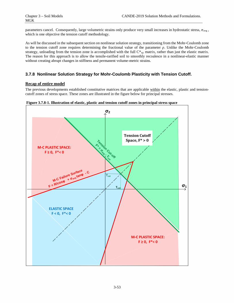
Chapter 3 – Soil Models CANDE-2019 Solution Methods and Formulations. MGK
3-53
parameters cancel. Consequently, large volumetric strains only produce very small increases in hydrostatic stress, σavg , which is one objective the tension cutoff methodology. As will be discussed in the subsequent section on nonlinear solution strategy, transitioning from the Mohr-Coulomb zone to the tension cutoff zone requires determining the fractional value of the parameter ρ. Unlike the Mohr-Coulomb strategy, unloading from the tension zone is accomplished with the full C*ep matrix, rather than just the elastic matrix. The reason for this approach is to allow the tensile-rarified soil to smoothly recoalesce in a nonlinear-elastic manner without creating abrupt changes in stiffness and permanent volume-metric strains.
3.7.8 Nonlinear Solution Strategy for Mohr-Coulomb Plasticity with Tension Cutoff.
Recap of entire model The previous developments established constitutive matrices that are applicable within the elastic, plastic and tension-cutoff zones of stress space. These zones are illustrated in the figure below for principal stresses. Figure 3.7.8-1. Illustration of elastic, plastic and tension cutoff zones in principal stress space
σ1
σ2
Tension CutoffSpace, F* > 0
M-C Failure Surface
F = R/cosφ + σavg tanφ - C
M-C PLASTIC SPACE: F ≥ 0, F*< 0
ELASTIC SPACEF < 0, F*< 0
Tcut
Tcut
Tension Cut-off
F* = σavg - T
cut
M-C PLASTIC SPACE: F ≥ 0, F*< 0

Chapter 3 – Soil Models CANDE-2019 Solution Methods and Formulations. MGK
3-54
The zone boundaries are defined by the Mohr-Coulomb yield function, F= 0 and the tension-cutoff yield function F*=0. For any arbitrary stress state, σ = <σx, σy, τxy>T, the zone to which this stress state belongs is determined by the following criteria;
(1) Elastic zone, F(σ) < 0 and F*(σ) < 0, with constitutive matrix, Cm = De (From Equation 3.7-2) (2) Plastic zone, F(σ) ≥ 0 and F*(σ) < 0, with constitutive matrix. Cm = De – Dp (From Equation 3.7-14) (3) Tension-cutoff zone, F*(σ) ≥ 0, with constitutive matrix, Cm = D*e – D*p (From Equation 3.7-24)
If the stress increment begins and ends in the same zone, then the constitutive matrix is as defined above. However, if the stress increment transitions from one zone to another during any load step, the parameters β and ρ enter into the constitutive matrix for general form expressed below. * *
m e p e pC = (1-ρ)(D -βD ) + ρ(D -βD ) Equation 3.7-25 where, β = fraction of stress increment in plastic zone (0 ≤ β ≤ 1)
ρ = fraction of stress increment in tension-cutoff zone (0 ≤ ρ≤ 1) As discussed next, convergence is dependent on achieving stable constitutive matrices for all elements, which in turn is dependent upon obtaining stabilized values for β and ρ.
Incremental-iterative procedure and convergence. CANDE, like most finite element programs, is a displacement based formulation wherein body loads and boundary loads are applied in a prescribed series of load steps. Each load-step requires the global assembly of the current estimate of the element stiffness matrices and a trial solution for displacement increments is obtained. Next, incremental strains are computed from the displacements and then incremental stresses are computed from the strains based on the current estimate of the stress-strain relationship. The new stress/strain state is used to update the stress-strain relationship and the whole solution process repeated until convergence is achieved. Repeated solutions within a load-step are called iterations. With the above understanding, the basic algorithm is developed at the element stress-strain level wherein all elements must converge during each load step before progressing to the next load step. The algorithm begins with the premise that a valid solution has been obtained for each element at the previous load step n-1, and the objective is to advance the solution to load step n. The constitutive matrix assigned to each individual element is dependent on the known stress-state defining the starting zone (elastic, plastic or tension-cutoff) and the ending zone of the trial stress increment. The following three sets of figures with tables offer complete set of conditions to define the constitutive matrix for all starting and ending stress states. Strictly speaking the non-hardening Mohr Coulomb model cannot sustain a stress state above the failure surfaces without producing unrestrained plastic flow. To avoid these singular constitutive matrices which produce infinitely large strains and displacements, the CANDE algorithm increases the elasticity matrices De by 1/1000 whenever β= 1.0. Likewise for De* whenever ρ = 1.0. Thus completely plastic responses are accompanied by large increases in strain magnitude, but not infinite NaN numbers.

Chapter 3 – Soil Models CANDE-2019 Solution Methods and Formulations. MGK
3-55
Figure 3.7.8-2 Case 1. Paths for Elastic Zone Start: F(σn-1) < 0 and F*(σn-1) < 0,
σ1
σ2
F = R/cosφ + σavg tanφ - C
F* = σavg - T
cut
Elastic-to-Elastic• β=0• ρ =0
Elastic-to-Plastic• β=(F(σn) - 0)/(F(σn) -F(σn-1 ) )• ρ=0
β
1-β
ρ
1-ρ
Elastic-to-Tension (Type 1 if F(σn’) < 0)• ρ=(F*(σn) - 0)/(F*(σn) -F*(σn-1 ) )• β = 0 , providing that F(σn’) < 0, Or• β = (F(σn’)–0)/(F(σn’)–F(σn)), if F(σn’) > 0 where σn’ = σn-1 + (1-ρ)Δσ
1-ρ
ρ
1-β β
Elastic-to-Tension (Type 2 if F(σn’) ≥ 0 )• ρ=(F*(σn) - 0)/(F*(σn) - F*(σn-1 ) )• β = (F(σn’) - 0))/(F(σn’) - F(σn-1) ) where σn’ = σn-1 + (1-ρ)Δσ
Trial incremental stress
Stress State
Ending Zone
Criteria for Ending Zone
Plasticity parameter β
Tension-cutoff parameter ρ
Constitutive matrix Cm
Elastic F(σn) < 0, and
F*(σn) < 0
0 0 De
Plastic F(σn) ≥ 0, and F*(σn) < 0
(F(σn)-0)/ (F(σn)-F(σn-1)) 0 De – βDp
Tension (Type 1)
F(σ’n) ≤ 0, and F*(σn) ≥ 0
0
(F*(σn)-0)/ (F*(σn)-F*(σn-
1)) (1-ρ)De +
ρ(D*e - D*p)
Tension (Type 2)
F(σ’n) > 0, and F*(σn) ≥ 0
(F(σ’n)-0)/ (F(σ’n)-F(σn-
1))
(F*(σn)-0)/ (F*(σn)-F*(σn-
1)) (1-ρ)(De - βDp) +
ρ(D*e - D*p)

Chapter 3 – Soil Models CANDE-2019 Solution Methods and Formulations. MGK
3-56
Figure 3.7.8-3 Case 2. Paths for Plastic Zone Start: F(σn-1) ≥ 0 and F*(σn-1) < 0
Stress State
Ending Zone
Criteria for Ending Zone
Plasticity parameter β
Tension-cutoff parameter ρ
Constitutive matrix Cm
Elastic F(σn) < F(σn-1),
and F*(σn) < 0
0 0 De
Plastic F(σn) ≥ F(σn-1), and F*(σn) < 0
1 0 De – Dp
Tension
F*(σn) ≥ 0 1
(F*(σn)-0)/ (F*(σn)-F*(σn-
1)) (1-ρ)(De - Dp ) +
ρ(D*e - D*p)
σ1
σ2
F = R/cosφ + σavg tanφ - CF* = σ
avg - Tcut
Trial incremental stress
Plastic-to-Plastic• β = 1• ρ = 0
Plastic-to-Elastic• β = 0• ρ = 0
ρ
Plastic-to-Tension• β = 1 over prortion (1-ρ)• ρ = (F*(σn ) - 0)/(F*(σn ) – F*(σn-1) )
1-ρ

Chapter 3 – Soil Models CANDE-2019 Solution Methods and Formulations. MGK
3-57
Figure 3.7.8-4 Case 3. Paths for Tension Zone Start: F*(σn-1) ≥ 0
Stress State
Ending Zone
Criteria for Ending Zone
Plasticity parameter β
Tension-cutoff parameter ρ
Constitutive matrix Cm
Elastic (Type 1)
F(σn) < 0, and F(σ’n) < 0. and F*(σn) < 0
0 (F*(σn-1)-0)/( F*(σn-1)-F*(σn))
(1-ρ)De + ρ(D*e-D*p)
Elastic (Type 2)
F(σn) < 0, and F(σ’n) ≥ 0, and F*(σn) < 0
(F(σ’n)-0)/ (F(σ’n)-F(σn)) (F*(σn-1)-0)/( F*(σn-1)-F*(σn))
(1-ρ)(De - βDp) + ρ(D*e - D*p)
Plastic F(σn) ≥ 0, and F*(σn) < 0
1
(F*(σn-1)-0)/( F*(σn-1)-F*(σn))
(1-ρ)(De - Dp) + ρ(D*e - D*p)
Tension
F*(σn) ≥ 0 0
1 D*e - D*p
σ1
σ2
F = R/cosφ + σavgtanφ - C
F* = σavg - T
cut
Trial incremental stress
Tension-to-Tension• β = 0• ρ = 1
1-ρ
ρ
Tension-to-Plastic• β = 1 over portion 1-ρ • ρ = (F*(σn-1)-0)/(F*(σn-1)-F*(σn))
Tension-to-Elastic (Type 1 if F(σn’)<0 )• ρ = (F*(σn-1)-0)/(F*(σn-1)-F*(σn))• β = 0 where σn’= σn-1+ρΔσ
ρ
1-ρ ρ
1-ρ
Tension-to-Elastic (Type 2 if F(σn’)>0 )• ρ = (F*(σn-1) - 0)/(F*(σn-1) - F*(σn))• β = (F(σn’)–0)/(F(σn’)–F(σn)), over
portion 1-ρ, and σn’= σn-1+ρΔσ
β 1-β

Chapter 3 – Soil Models CANDE-2019 Solution Methods and Formulations. MGK
3-58
The logic associated with above figures and charts produce a fairly robust algorithm that usually converges, even when large strains occur due to stress states that are imposed above the failure surfaces. CANDE deduces convergence when the constitutive matrices of all elements are stabilized i.e., remains essentially constant over two iterations. Sometimes elements may chatter, meaning that the element oscillates between one end state and another. When this occurs CANDE has been equipped with logic to choose the most likely state. However, there are times when Mohr-Coulomb does not converge, when this occurs the following suggestions are offered:
1. Set ITMAX = -50 in line A-1. The minus sign forces CANDE to continue processing each load step even if convergence is not achieved.
2. Set IWRT = 4 in line C-2 of Level 3 (or appropriate C-line in Level 2 options ). This command provides a trace printout in the CANDE output report for each iteration of all the Mohr-Coulomb elements showing the convergence errors. 3. Rather than applying increments of force to represent live loads, apply displacement increments. The equivalent incremental force can be determined by applying the displacement increment through a link element.
This completes the Mohr-Coulomb model development.

Chapter 3 – Soil Models CANDE-2019 Solution Methods and Formulations. MGK
3-59
3.8 Comparison of Duncan/Selig and Mohr/Coulomb Soil Models The remainder of this soil-model Chapter is devoted to a comparative study between the Duncan/Selig and Mohr/Coulomb soil models. The comparative study includes the following components.
1. Experimental data suite. Summary tables of experimental results for Cooks Bayou sand are provided to document the data base, which includes three triaxial tests, one hydrostatic test, and one confined compression test. All data is for loading, not unloading.
2. Parameter identification. Model parameters for the Mohr/Coulomb and Duncan/Selig model are computed to
best fit the triaxial data and parameter identification techniques are discussed.
3. Comparative plots. The Mohr/Coulomb and Duncan/Selig model predictions are plotted against the corresponding experimental data and the models are judged accordingly.
Each of the above components is addressed, in turn, in the following subsections.
3.8.1 Experimental Data Suite Experimental test data used in this study was generated by the US Army Core of Engineers at the Waterways Experiment Station in the 1970s using vintage triaxial testing equipment. All soil samples were taken from a natural sand quarry called Cook’s Bayou wherein the sand is fairly well graded with a small amount of fines. Soil samples were tested in dry conditions with initial density of 112 pcf. Although the test data is old, it is considered very reliable. The suite of experimental tests includes three standard tri-axial tests with confining pressures of 25, 50 and 100 psi as presented in Table 3.8.1-1 wherein all responses are referenced to zero after the confining pressure is applied so that deviator stress is equal to axial stress. The deviator stress at failure is highlighted in yellow, which is closely correlated with the radial stain approaching ½ of the axial stain, i.e., Poisson ratio approaching 0.5. TABLE 3.8.1-1. Standard tri-axial test data for confining pressures = 25, 50 and 100 psi
Confining stress = 25 psi
Confining stress = 50 psi
Confining stress = 100 psi
Axial Stress
psi
Axial Strain
%
Radial Strain
%
Axial Stress
psi
Axial Strain
%
Radial Strain
%
Axial Stress
psi
Axial Strain
%
Radial Strain
% 0.00 0.00 0.00 0.00 0.00 0.00 0.00 0.00 0.00
14.80 0.41 -0.04 13.11 0.33 -0.04 25.49 0.63 -0.04 31.80 0.94 -0.18 30.14 0.65 -0.11 76.45 1.91 -0.22 48.78 1.57 -0.40 64.17 1.74 -0.37 127.32 3.33 -0.58 65.72 2.48 -0.80 98.10 3.23 -0.91 178.02 5.04 -1.24 82.58 3.92 -1.54 131.85 5.61 -1.87 228.31 7.31 -2.48 99.18 7.40 -3.33 164.82 10.30 -4.83 277.73 10.75 -4.86
110.84 13.01 -6.40 176.00 13.95 -7.18 310.07 13.55 -6.95 113.00 14.09 -6.99 - - - 314.00 17.08 -9.57
Next, Table 3.8.1-2 contains the results of a hydrostatic test on Cook’s Bayou sand. The right column is the computed secant bulk modulus determined by dividing the current hydrostatic pressure by the current volumetric strain.

Chapter 3 – Soil Models CANDE-2019 Solution Methods and Formulations. MGK
3-60
TABLE 3.8.1-2 Hydrostatic test data for Cook’s Bayou sand
Hydrostatic Pressure psi
Volume change %
Secant Bulk Modulus psi
0 0 -- 20 1.62 1235 45 2.73 1648 70 3.53 1983 95 4.49 2116
120 5.12 2344 145 5.67 2557 170 6.23 2729 195 6.66 2928 220 7.12 3090 245 7.53 3254
Lastly, Table 3.8.1-3 contains the experimental results for a uniaxial strain test, also called a confined compression test, also called a K0 test. For this experiment a uniform hydrostatic pressure is applied, then axial stress is increased until the observed radial strain is zero. By definition, the secant confined modulus (Ms) is equal to the total axial stress divided by the total axial strain, and the lateral coefficient (K0) is the radial stress divided by the axial stress. These calculations are shown in the last two columns, respectively. TABLE 3.8.1-3. Uniaxial strain data for Cook’s Bayou sand .
Total axial stress psi
Total radial stress psi
Total axial strain %
Secant Confined Modulus
psi
Lateral Coefficient, K0
- 0 0 0 -- --
25.2 8 1.36 1853 0.317 50.71 18 2.25 2254 0.355 78.59 28 3.15 2495 0.356
129.78 48 4.31 3011 0.370 204.9 73 5.72 3582 0.356
273.24 98 6.8 4018 0.359 345.48 123 7.89 4379 0.356 413.66 148 8.79 4706 0.358 481.5 173 9.65 4990 0.359
Subsequently, the tabular data in the above tables will be shown as plots versus soil model predictions. However, the raw data in the above tables will be useful to researches to extend this study to include other soil models.
3.8.2 Parameter Identification The tri-axial test data in Table 3.8.1-1 is used to determine values for the elastic parameters E and ν, the Mohr/Coulomb parameters c and φ, and all parameters for Duncan Young’s modulus. Hydrostatic test data in Table 3.8.1-2 is used to determine Selig bulk modulus parameters, Bi and εu. Uniaxial strain data in Table 3.8.1-3 is not used for parameter identification; hence, this data serves as a blind test for the predictive capability of each soil model. The three deviatoric failure stresses highlighted in Table 3.8.1-1 (113, 176, and 314 psi) are used to construct Mohr circles for each failure state as illustrated in the figure below. In this case, the Mohr-Coulomb failure surface forms a straight line with c = 12.5 psi and φ = 35.60, these parameters apply to both the Mohr/Coulomb and Duncan/Selig models with Δφ = 0.

Chapter 3 – Soil Models CANDE-2019 Solution Methods and Formulations. MGK
3-61
FIGURE 3.8.2-1. Mohr-Coulomb failure surface determined from tri-axial test data.
Initial values for Young’s modulus are determined by dividing initial axial stress by initial axial strain, which produces E = 3069, 3972 and 4046 psi for each confining pressures, respectively. For the linear-elastic and the Mohr/Coulomb elastoplastic soil models, the average value E = 3876 psi is assigned to Young’s modulus. Likewise, Poisson ratio is ν = 0.30 is the average result from all ratios of radial strain to axial strain. Table 3.8.2-1 summarizes the parameter values used for the linear elastic and Mohr/Coulomb elastoplastic models. TABLE 3.8.2-1 . Linear Elastic and Mohr/Coulomb parameters for Cooks Bayou Sand.
Parameter Name
Symbol Values based on best fit to data
Cohesion strength c 12.5 psi Internal friction angle φ 35.60 Young’s modulus E 3876 psi Poisson’s ratio ν 0.30
Initial Young’s modulus for the Duncan/Selig model is defined by a power law and the best fit to the initial moduli data is K = 238 and n = 0.0823 so that the initial modulus may be expressed as Ei = 3500(σ3/14.7)0.0823. Finally, the bulk modulus function is determined by least-squares best fit to hydrostatic data in Table 3.8.1-2 resulting in Bi = 1263 psi and ϵu = 0.1177%. Table 3.8.2-2 summarizes the 8 parameter values for the Duncan/Selig soil model.
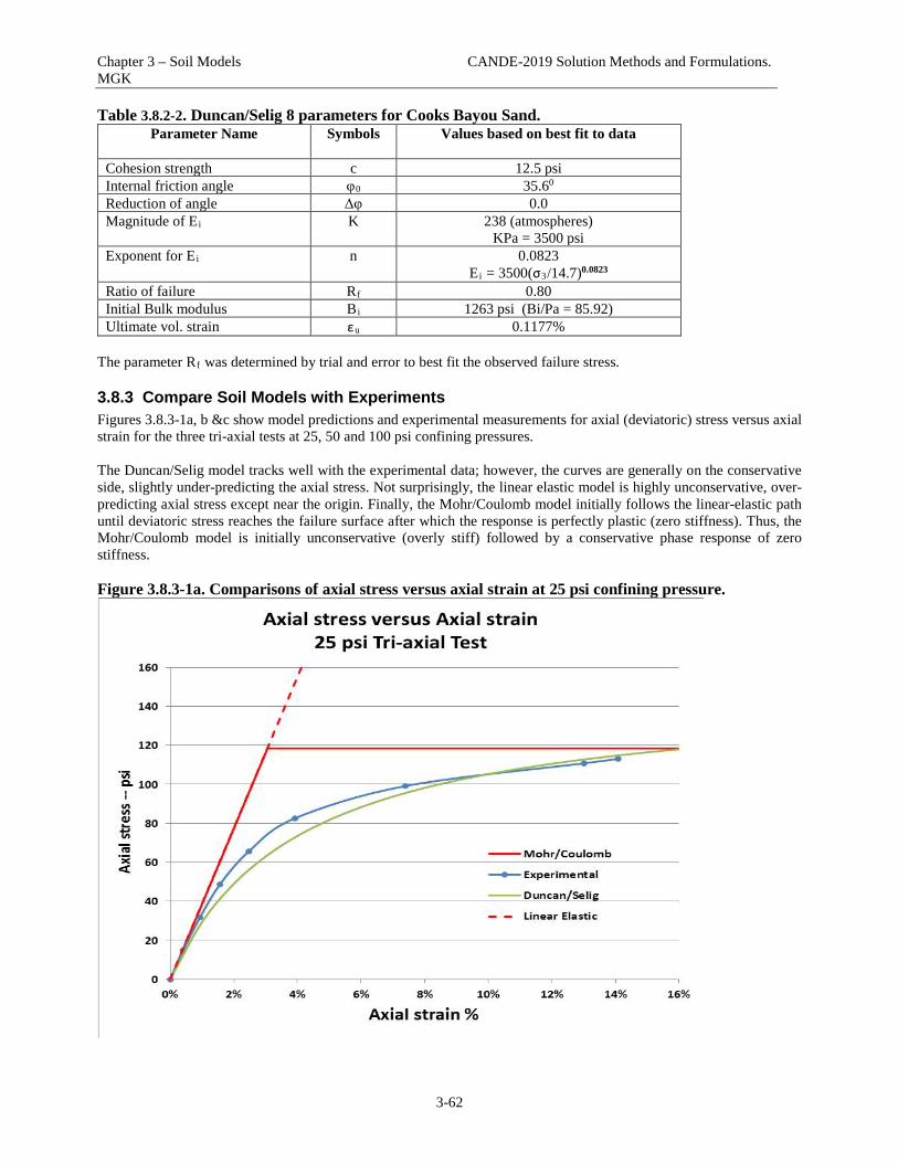
Chapter 3 – Soil Models CANDE-2019 Solution Methods and Formulations. MGK
3-62
Table 3.8.2-2. Duncan/Selig 8 parameters for Cooks Bayou Sand. Parameter Name
Symbols Values based on best fit to data
Cohesion strength c 12.5 psi Internal friction angle φ0 35.60 Reduction of angle Δφ 0.0 Magnitude of Ei K 238 (atmospheres)
KPa = 3500 psi Exponent for Ei n 0.0823
Ei = 3500(σ3/14.7)0.0823 Ratio of failure Rf 0.80 Initial Bulk modulus Bi 1263 psi (Bi/Pa = 85.92) Ultimate vol. strain εu 0.1177%
The parameter Rf was determined by trial and error to best fit the observed failure stress.
3.8.3 Compare Soil Models with Experiments Figures 3.8.3-1a, b &c show model predictions and experimental measurements for axial (deviatoric) stress versus axial strain for the three tri-axial tests at 25, 50 and 100 psi confining pressures. The Duncan/Selig model tracks well with the experimental data; however, the curves are generally on the conservative side, slightly under-predicting the axial stress. Not surprisingly, the linear elastic model is highly unconservative, over-predicting axial stress except near the origin. Finally, the Mohr/Coulomb model initially follows the linear-elastic path until deviatoric stress reaches the failure surface after which the response is perfectly plastic (zero stiffness). Thus, the Mohr/Coulomb model is initially unconservative (overly stiff) followed by a conservative phase response of zero stiffness. Figure 3.8.3-1a. Comparisons of axial stress versus axial strain at 25 psi confining pressure.

Chapter 3 – Soil Models CANDE-2019 Solution Methods and Formulations. MGK
3-63
Figure 3.8.3-1b. Comparisons of axial stress versus axial strain at 50 psi confining pressure.
Figure 3.8.3-1c. Comparisons of axial stress versus axial strain at 100 psi confining pressure.
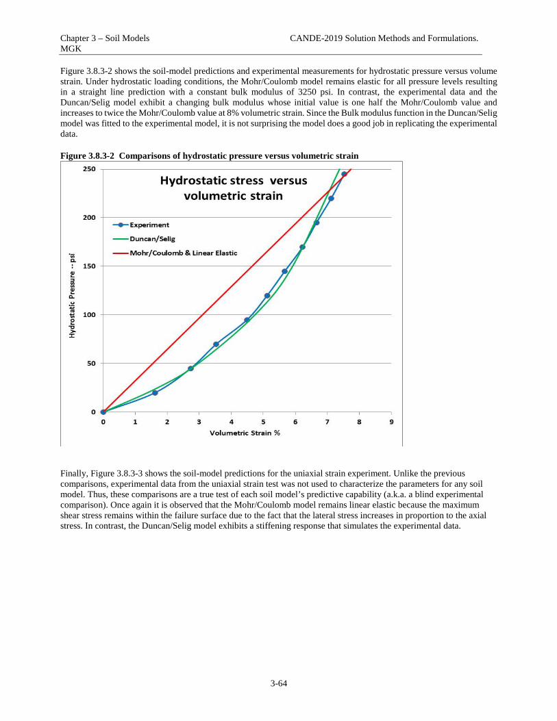
Chapter 3 – Soil Models CANDE-2019 Solution Methods and Formulations. MGK
3-64
Figure 3.8.3-2 shows the soil-model predictions and experimental measurements for hydrostatic pressure versus volume strain. Under hydrostatic loading conditions, the Mohr/Coulomb model remains elastic for all pressure levels resulting in a straight line prediction with a constant bulk modulus of 3250 psi. In contrast, the experimental data and the Duncan/Selig model exhibit a changing bulk modulus whose initial value is one half the Mohr/Coulomb value and increases to twice the Mohr/Coulomb value at 8% volumetric strain. Since the Bulk modulus function in the Duncan/Selig model was fitted to the experimental model, it is not surprising the model does a good job in replicating the experimental data. Figure 3.8.3-2 Comparisons of hydrostatic pressure versus volumetric strain
Finally, Figure 3.8.3-3 shows the soil-model predictions for the uniaxial strain experiment. Unlike the previous comparisons, experimental data from the uniaxial strain test was not used to characterize the parameters for any soil model. Thus, these comparisons are a true test of each soil model’s predictive capability (a.k.a. a blind experimental comparison). Once again it is observed that the Mohr/Coulomb model remains linear elastic because the maximum shear stress remains within the failure surface due to the fact that the lateral stress increases in proportion to the axial stress. In contrast, the Duncan/Selig model exhibits a stiffening response that simulates the experimental data.

Chapter 3 – Soil Models CANDE-2019 Solution Methods and Formulations. MGK
3-65
Figure 3.8.3-3 Comparisons of axial stress versus axial strain in confined compression.
The overall conclusion from all the above comparisons is that the Duncan/Selig soil-model performs the best in replicating soil loading behavior. The Mohr/Coulomb performs exactly like the linear elastic model for hydrostatic and confined compression loading. For triaxial tests (deviatoric stress loading), the Mohr Coulomb model responds with a sharp dogleg (elastic-perfectly plastic), which is a crude approximation to the gradually decreasing stiffness exhibited by the experimental data. A more profound question is, “What difference does the three soil models make when it comes to predicting the distress in culvert installations?” This question is studied and answered for corrugated metal, reinforced concrete, and plastic pipe in deep and shallow burial in Reference 28. The bottom-line answer is that the Duncan/Selig model is preferable because it leads to conservative predictions.

Chapter 5 – Large Deformations and Buckling CANDE-2019 Solution Methods and Formulations. MGK
4-1
INTERFACE AND LINK ELEMENT This chapter presents the development of the interface element and the link element, which have similar derivations based on constraint equations. The interface element is a friction-contact surface that simulates frictional slippage, separation, and re-bonding of two bodies mating at a common interface and subsequently deforming under an arbitrary static loading schedule. Constraint equations between mating pairs of nodes and the general principle of virtual work are used to formulate the interface element for a finite element solution methodology. The practical application of the interface elements is to mimic the behavior of the interface between the culvert exterior and backfill soil by simulating frictional slippage of the soil over the culvert wall during the backfilling operations. Similarly, the model is useful for simulating the slippage of backfill soil along trench walls for steep walled trench installations. More recently, the interface element formulation was extended to include the option of assigning an initial gap between the contact bodies. In general the interface element requires a nonlinear solution process to determine the correct interface state (fixed, slip or free) and the correct interface forces. Link elements are special constraints placed on degrees of freedom associated with two independent nodes. It is a simple linear operation. For example, the “rigid link” element enforces two beam nodes to experience the same x and y translation and a rotation, as if the beam nodes formed a welded connection. As another example, the “pinned” link element only enforces the same x and y translation without constraining rotations. Still another example is the so-called composite link element that may be used to join two parallel beam groups to act as a single beam group with a pre-defined percentage of composite action. Perhaps the greatest utility of the link elements is the so-called element depth option that is triggered by a user-defined load step. Simply put, his means the link element forces are removed and the element no longer exists when the load step number reaches the user-specified death step number. The link element death option has many practical applications such as removing temporary construction bracing, creating void openings in soil zones, and simulating the deterioration of structural segments.
4.1 Interface Element Introduction CANDE’s interface element dates back to its original development in 1976, which is documented in Reference 1 and published in the open literature in Reference 24. Today, the interface element remains as originally developed with a few minor modifications to enhance convergence. Engineering literature contains a variety of interface element formulations; however, they can generally be classified as either a stiffness approach (e.g. directionally stiff elements) or a constraint approach typically formulated with the use of Lagrange multipliers. The constraint approach is used in this development, however rather than using Lagrange multipliers, the development is based on a novel extension of virtual work, which in itself became a contribution to FEM technology. Motivations for adopting the constraint approach include, avoidance of numerical round-off problems inherent in the stiffness approach, direct control of interface forces and relative movements, accuracy, and ease of FEM implementation. The interface element is capable of responding to a general step-by-step loading history, such that tensile separation, frictional sliding, or complete bonding (or re-bonding) is possible during any load step. Two nodes, one on either side of an interface, defined by the interface angle, are used to establish the interface element along with a third “dummy node” to represent interface forces. By selectively applying constraint equations to the interface nodes in an incremental-iterative solution procedure, the behavior of a contact-friction interface is simulated. Two computational advantages are inherent in the interface element. First, unlike the traditional Lagrange-multiplier method that requires a minimization principle, the virtual work formulation is not restricted to conservative systems. Secondly, the formulation results in an element 'constraint matrix' and element 'load vector' analogous to a typical element stiffness matrix and load vector. Thus, the interface element can be assembled into the global equations by standard techniques.

Chapter 5 – Large Deformations and Buckling CANDE-2019 Solution Methods and Formulations. MGK
4-2
4.2 Interface Virtual Work and Constraint Equations In Chapter 1, the traditional virtual work formulation is presented without constraints resulting in the classical, stiffness-based finite equations expressed in a scalar virtual work statement repeated here as, Tˆ ˆδu (KΔu - ΔP) = 0 Equation 4.2-1 where, ˆΔu = incremental unknown nodal displacements K = current global stiffness matrix (generally nonlinear) ΔP = incremental load vector. Since δuT is an arbitrary virtual displacement, the satisfaction of Equation 4.2-1 requires that KΔu = ΔP, usually solved iteratively to find displacements. If Equation 4.2-1 represented a finite element model of two separate bodies initially in contact at node pairs as suggested in Figure 4.2-1, then the bodies can deform independently resulting in overlapping and/or separation along the interface. At the other extreme, if the node pairs at the interface are constrained to move together, a completely bonded response is obtained. Between these two extremes, a slipping response can be obtained by constraining only the displacements normal to the interface at each node pair. Figure 4.2-1 Idealization of two bodies with initially mating node pairs along interface
Body A
Body B
Node pairs

Chapter 5 – Large Deformations and Buckling CANDE-2019 Solution Methods and Formulations. MGK
4-3
4.2.1 Constraint equations general form To achieve the above, the immediate objective is to incorporate an arbitrary set of constraint equations into a global virtual work statement. Formally, any set of algebraic nodal point constraint equations can be expressed as: ˆˆˆCΔu - Δa = 0 Equation 4.2-2 where, C = constraint coefficient matrix ˆΔu = subset of nodal degrees of freedom being constrained ˆΔa = vector of specified constants (for example, displacement gaps)
0 = vector of zeroes, one zero for each constraint equation. To fix ideas by means of a simple example, suppose it is desired to constrain one node in body A to be glued (fixed) to the partner node in body B with no displacement gap between the node pair. In this case, Equation 4.2-2 would be written in expanded notation as,
Ax
Ay
Bx
By
uu-1 0 1 0 0 0
- = u0 -1 0 1 0 0u
In the above example we are simply imposing the two constraint equations, uAx = uBx and uAy = uBy, which forces the x and y displacement component of the node in body A to be equal to those of the paired node in body B. Associated with each constraint equation, there exists an unknown internal constraint force λ enforcing the constraint. For convenience, Equation 4.4-2 can be expressed in a scalar (work) form as: Tˆ ˆˆδλ (CΔu - Δa) = 0 Equation 4.2-3 where, λ = vector of interface constraint forces, one force component for each constraint equation. Since ˆδλ is an arbitrary variation of the constraint force vector, Equation 4.2-3 is satisfied if and only if the constraint equations are satisfied. As yet the virtual work of constraint forces has not been established or defined. To this end, we argue that the internal constraint forces produce internal virtual work when the constraint is given a small virtual movement (variation) as follows. T T T
constraintˆ ˆˆˆ ˆVW = δ(CΔu - Δa) Δλ = δu C Δλ Equation 4.2-4
In the above definition for the incremental virtual work of constraints, we assume the system is equilibrium at load step i and moves to a new equilibrium position at load step i+1 consistent with the incremental constraint equations, which in turn generate incremental constraint forces, Δλ. When the constraints are given a small virtual disturbance (variation), the constraint forces perform virtual work as they move with the virtual disturbance. Physically, this is analogous to imposing constraints with stiff springs between node pairs wherein the internal spring force corresponds to the constraint force. However, in this case the constraint forces are primary unknowns.

Chapter 5 – Large Deformations and Buckling CANDE-2019 Solution Methods and Formulations. MGK
4-4
4.2.2 Global virtual work statement with constraints With the above understandings, we complete the formulation by adding the internal virtual work of constraints (Equation 4.2-4) to the standard virtual work statement in Equation 4.2-1 and append the constraint requirement in Equation 4.2-3 to get the general virtual work statement including constraints.
T Tˆ ˆδu Δu ΔPK C - = 0ˆ ˆ ˆΔaC 0δλ Δλ
Equation 4.2-5
Since the virtual displacements and virtual constraint forces are arbitrary, the virtual work statement leads to the following global system of equations.
T u PK C
= ˆ aC 0 λ
∆ ∆ ∆∆
Equation 4.2-6
The coupled set of global matrix equations is to be solved for nodal displacements and constraint forces. Note that the separate partitioning of the global system into Δu and Δλ is a mere formality and not required in actual global assembly.
4.2.3 General element constraint matrix and load vector Recalling that the global stiffness equations are formed from the summation element stiffness matrices and load vectors based on the element’s contributions to total virtual work, we can in the same manner construct an element constraint matrix and load vector based on the constraint element’s contribution to the virtual work as shown below.
T Te ee
contstraintelement e ee e
ˆˆ ˆδu Δu0 C 0δV = - ˆ ˆ ˆC 0 Δaδλ Δλ
Equation 4.2-7
Since the above expression represents the contribution of a general constraint element to the global virtual work statement given by Equation 4.2-5, the element-level constraint matrix and load vector are established as follows.
T
e
e
0 CC* =
C 0
Equation 4.2-8
e
0f = a
∆
Equation 4.2-9
where, C* = symmetric element constraint matrix, dimension (n+m) x (n+m) eC = constraint coefficient matrix for element, dimension m x n
f = incremental load vector of zeros and displacement gaps, dimension n+m ˆΔa = specified incremental displacement gaps, dimension m m = number of constraint equations associated with element (m = 2 for interface element) n = number of constrained degrees of freedom within element (n= 4 for interface element) Just as the global stiffness matrix is assembled by a summation of element stiffness matrices k*, the global constraint matrix is assembled by a summation of element constraint matrices C*. Similarly, the global constraint load vector is assembled by a summation of element load vectors f .

Chapter 5 – Large Deformations and Buckling CANDE-2019 Solution Methods and Formulations. MGK
4-5
4.3 Interface Element Matrix and Load Vector To specialize the foregoing to friction-contact interfaces, we assume that any interface can be modeled as a sequence of node pairs (Figure 4.2-1), so that attention can be focused on a single node pair that forms an interface element.
4.3.1 Definition of interface element The interface element is composed two nodes on either side of a common interface plus an interior node (a stand-alone node K) that represents interface forces. Figure 4.3.1-1 shows an exploded view of the interface element. Figure 4.3.1-1 Interface element exploded view defining normal and tangential directions
Here, the interface element is defined in the local n, s coordinates, rotated φ degrees from the global x, y coordinate system. Node I belongs to the body on one side of the interface and Node J belongs to the body on the other side of the interface. Node I and J are initially assigned to the same x, y coordinate location prior to loading. The positive normal direction is in the direction of travel from node I to node J. Nodal displacement components in the n-s system are marked with a prime to distinguish them from the unprimed components in the x-y system. Physical properties assigned to the interface element are listed below.
μ = coefficient of friction (Coulomb type) β = tensile rupture force (typically = 0) φ = angle of the interface normal with respect to x-axis

Chapter 5 – Large Deformations and Buckling CANDE-2019 Solution Methods and Formulations. MGK
4-6
The coefficient of friction and tensile rupture force are discussed subsequently, however it should be evident that if these properties are assigned very large numbers the interface will remain bonded (fixed) regardless of the interface angle and internal forces.
4.3.2 Incremental and total responses (notation) As with all developments in this manual, the interface element is an incremental relationship from load step i to load step i+1. Letting the symbol q represent any interface response, we adopt the following notation for incremental relationships. i+1 iq = q + Δq Equation 4.3-1 where, i+1q = total response at load step i+1
iq = total response at load step i Δq = incremental response from step i to i+1 The following list defines interface response notation represented by the symbol q
Iu ′ = displacement of node I in the normal direction.
Ju′ = displacement of node J in the normal direction
Iv′ = displacement of node I in the tangent direction.
Jv′ = displacement of node J in the tangent direction.
nλ = normal force between node I and J
sλ = tangent force between node I and J
Iu = displacement of node I in the global x direction.
Ju = displacement of node J in the global x direction
Iv = displacement of node I in the global y direction.
Jv = displacement of node J in the global y direction.
nd = interface gap distance in normal direction
sd = interface gap distance in tangent direction Interface gap distances are illustrated in the figure below for load step i wherein the two bodies have separated at nodes I and J producing normal and tangential gaps between the nodes.

Chapter 5 – Large Deformations and Buckling CANDE-2019 Solution Methods and Formulations. MGK
4-7
Figure 4.3.1-1 Interface element in separated state at load step i.
The total normal gap and the total tangential gap at load step i are determined by the difference of nodal displacement components in the n-s coordinates as given below. i i i
n J Id = u - u′ ′ Equation 4.3-2a i i i
s J Id = v - v′ ′ Equation 4.3-2b
4.3.3 Element constraint matrices and load vectors for three interface states. We now identify three 'interface states' that may be imposed during a load step depending on the current responses of the interface element. The three states are called fixed, slip, and free. In each case we will define the element constraint matrix and load vector. Fixed State. The fixed state means that nodes I and J are constrained to move during the load step such that specified incremental gaps will occur in the normal and tangent direction (usually the incremental gaps are specified to be zero). In the local n-s coordinates system the fixed state is expressed with the following two constrain equations. I J-Δu + Δu = Δa′ ′ Equation 4.3-3 I J-Δv + Δv = Δb′ ′ Equation 4.3-4 where, a∆ = specified normal gap increment (often zero)
b∆ = specified tangential gap increment (often zero)
Since the global equations require that displacement components be expressed in x-y coordinates, the primed displacement components are transformed to x-y displacement components by standard coordinate transformation techniques so that the above constraint equations become,

Chapter 5 – Large Deformations and Buckling CANDE-2019 Solution Methods and Formulations. MGK
4-8
I
I
J
J
ΔuΔv-cosφ -sinφ cosφ sinφ Δa
= Δusinφ -cosφ -sinφ cosφ ΔbΔv
Equation 4.3-5
Here the 2x4 matrix is the constraint coefficient matrix Ce that is imbedded in the symmetric element constraint matrix C* defined by Equation 4.2-8. The right hand side is the specified incremental gap vector for the element load vector defined in Equation 4.2-9. If Δa and Δb are both specified zero, then the normal gap and tangential gap do not change during the load step, i.e. both nodes experience identical displacement increments. If, on the other hand, we wish to return the nodes to their initial position (no gaps), we specify Δa and Δb equal to the total displacement gaps defined in Equations 4-3-2a,b. The fixed state is summarized in the top portion of Table 4.3.3-1, which explicitly defines the element constraint matrix C* and the element load vector. These may be assembled in the global system just like element stiffness matrix. Table 4.3.3-1 Element constraint matrix C* (6x6) and load vector f (6x1) for three interface states.
State
Iu∆
Iv∆
Ju∆
Jv∆
nλ∆
sλ∆ f
(load)
Fixed
0 0 0 0 -c s 0 0 0 0 0 -s -c 0 0 0 0 0 c -s 0 0 0 0 0 s c 0 -c -s c s 0 0 Δa s -c -s c 0 0 Δb
Slip
0 0 0 0 -c 0 -sΔT 0 0 0 0 -s 0 cΔT 0 0 0 0 c 0 sΔT 0 0 0 0 s 0 -cΔT -c -s c s 0 0 Δa 0 0 0 0 0 1 ΔT
Free
0 0 0 0 0 0 cΔN - sΔT 0 0 0 0 0 0 sΔN + cΔT 0 0 0 0 0 0 -cΔN + sΔT 0 0 0 0 0 0 -sΔN - cΔT 0 0 0 0 1 0 ΔN 0 0 0 0 0 1 ΔT
c = cosφ, and s = sinφ Slip State. The slipping state is defined by constraining the normal displacement increments of nodes I and J such that a specified incremental gap will occur in the normal direction during the load increment. The tangential displacement constraint is suppressed and replaced with a specification for the incremental interface force in the tangent direction. Specifically, the slip state is expressed with the following constraint equation and force equation in the n-s system. I J-Δu + Δu = Δa′ ′ Equation 4.3-6 sΔλ = ΔT Equation 4.3-7

Chapter 5 – Large Deformations and Buckling CANDE-2019 Solution Methods and Formulations. MGK
4-9
where, Δa = specified normal gap increment (often zero) ΔT = specified increment of tangential force between nodes I and J
Since other types of elements share nodes I and J, the n-s displacement components must be transformed to the common x-y system for global assembly and solution. Thus the above constraint equation is transformed to x-y system as shown below.
( )
I
T I
J
J
ΔuΔv
-cosφ -sinφ cosφ sinφ = ΔaΔuΔv
Equation 4.3-8
With regard to the force equation (Equation 4.3-7), it may be retained in the n-s coordinate system because the dummy node K containing the interface forces is not shared with any other element. Whenever we suppress a constraint and specify Δλs = ΔT, we must also assign a positive ΔT force to node I and a negative ΔT force to node J thereby effecting the interface force on the nodes. Also we must transform these forces to x-y system for proper assembly in the global load vector as shown in the load vector column in Table 4.3.3-1. The slipped state is summarized in the central portion of Table 4.3.3-1. Here the C* matrix contains one constraint equation and force equation (λs = T), wherein the matrix size remains 6 x 6 for computational convenience. As discussed above, the load vector includes force components at nodes I and J from the specified interface force, ΔT. To simulate a friction-contact interface, Coulomb-type friction is assumed so that the maximum possible interface tangent force in advancing from load step i to i+1 is a function of the normal compressive force and given by,
i+1 i+1 i+1n sF = μ λ sgn(λ ) Equation 4.3-9
where, i+1F = maximum Coulomb frictional force at step i+1 (signed) μ = coefficient of friction
i+1
si+1s i+1
s
+1, for λ > 0sgn(λ ) =
-1, for λ < 0
With the above understanding, a frictional slipping interface requires that the specified incremental tangent force from load step i to i+1 satisfy the equilibrium condition as written below. i+1 i
sΔT = F - λ Equation 4.3-10 where, i
sλ = known tangential interface force at load step i. Of course, ΔT is recomputed by iterating within the load step until two successive values of Fi+1 are acceptably close, say within 1%. Free State. The free state is defined by suppressing both constraint equations and specifying the normal and tangent interface force increments as shown below. nλ = N∆ ∆ Equation 4.3-11 sΔλ = ΔT Equation 4.3-12

Chapter 5 – Large Deformations and Buckling CANDE-2019 Solution Methods and Formulations. MGK
4-10
where, ΔN = specified increment of normal force between nodes I and J ΔT = specified increment of tangential force between nodes I and J Again, the above force equations may be expressed in the n-s coordinate system because the dummy node K containing the interface forces is not shared with any other element. In addition, the specified interface forces ΔN and ΔT must be assigned to nodes I and J, positive for node I and negative for node J. Also these forces must be transformed to x-y system for proper assembly in the global load vector. The free state is summarized in the bottom portion of Table 4.3.3-1. Here the C* matrix is all zeros except C* (5,5) = C* (6,6) = 1 that enforces the equations Δλn = ΔN and Δλs = ΔT. Again, the matrix size remains 6 x 6 for computational convenience. Lastly, the load vector includes x-y force components at nodes I and J from the specified interface forces.
4.4 Interface Nonlinear Solution Strategy The problem is posed as follows. We assume we know the interface solution at end of load step i, which includes converged solutions for the following accumulated interface responses.
i in sλ , λ = total interface normal and tangent interface forces at end of load step i.
i in sd , d = total interface normal and tangent displacement gaps at end of load step i.
We seek to determine an incremental solution ( Δλn, Δλs, Δdn, and Δds) to achieve a valid solution for the total interface responses at the end of load step i+1 computed as follows. i+1 i
n n nλ = λ + Δλ Equation 4.4-1
i+1 is s sλ = λ + Δλ Equation 4.4-2
i+1 in n nd = d + Δd Equation 4.4-3
i+1 is s sd = d + Δd Equation 4.4-4
By a valid solution we mean the physical compatibility and equilibrium conditions of the contact-friction interface are satisfied. In general the valid solution must be determined iteratively wherein a particular state (fixed, slip, or free) is assumed and solved to obtain a trial solution. The trial solution is used to determine if the assumed state is correct, and if not, what state is more likely to be correct. At the same time, the trial solution is used to estimate new parameters for the trial load vector associated with trial interface state as listed below.
• Fixed state load parameters = Δa, Δb • Slip state load parameters = Δa, ΔT • Free state load parameters = ΔN, ΔT
Recall that Δa and Δb are specified incremental displacement gaps in normal and tangential directions, respectively, and ΔN and ΔT are specified incremental interface forces in normal and tangential directions, respectively.
4.4.1 Selecting a new trial interface state Table II offers an exhaustive set of physical criteria to test the validity of an assumed state. The table may be viewed as a 3 x 3 decision matrix wherein the previously assumed state forms rows and the new candidate states form columns.

Chapter 5 – Large Deformations and Buckling CANDE-2019 Solution Methods and Formulations. MGK
4-11
Table 4.4.1-1 Decision matrix for selecting new trial interface state during iteration cycle from load step i to i+1
New trial state → Previous trial state ↓
Fix
↑
Slip
↑
Free
↑
(1) Fix →
i+1 i+1 i+1
n sλ < β and λ < F
i+1 i+1 i+1n sλ < β and λ > F
i+1
nλ > β
(2) Slip →
i+1 i+1
n sλ < β and Δd F < 0
i+1 i+1n sλ < β and Δd F > 0
i+1
nλ > β
(3) Free →
i+1
nd < 0
--
i+1nd > 0
To illustrate the decision matrix, if the previously assumed state was fixed, then row 1of the decision matrix is entered from the left. The first query determines if the fixed state is correct by checking if the current normal interface force is compressive (or less than the tensile rupture force β) and the magnitude of the tangential force is less than the current frictional resistance calculated from Equation 4.3-9. If both of these inequalities are satisfied than the fixed state is correct, and the fixed state is assumed for the next iteration. Otherwise, we proceed to query the slip conditions to see if the tangential force exceeds the frictional resistance while the interface normal force is compressive. If both of these conditions are satisfied, then we select the slip sate for the next iteration. The only remaining possibility is that the normal force exceeds the tensile resistance, implying the interface is prone to separate so that we choose the free state for the next iteration. If the previous state was slip, we enter row 2 of the decision matrix to determine the most likely state for the next iteration. The first query determines whether or not we should shift to a fixed state based on the conditions that the normal force remains compressive, but there is a change in the direction of relative slip determined by the sign of the product of the slip increment, Δds, and the signed value of frictional resistance from Equation 4.3-9. This somewhat subtle argument is based on the observation that relative slip movement cannot reverse its direction until the passive frictional force totally reverses its direction. Therefore, a fixed state for the next iteration is assumed. On the other hand, if the product of the slip increment and the frictional resistance is positive (that is, they have the same sign), then we assume the slip state remains correct for the next iteration. The only remaining possibility is that the normal force exceeds the tensile resistance implying the interface is prone to separate so that we choose the free state for the next iteration. Lastly if the previous state was free, we enter row 3 to determine whether or not to remain in the free state or shift to a fixed state for the next iteration. We shift to a fixed state if the current normal gap is less than zero meaning that the two bodies have incorrectly penetrated each other at this point. Otherwise, we remain in the free state for the next iteration. Note that row 3 does not provide a direct path from a free state to a slip state. This does not mean a slip state cannot be reached from a free state; it simply means a slip state must be reached by the iterative path, free to fix to slip. Recapping, the decision matrix provides the choice for the next assumed state, thereby dictating the form of the element constraint matrix C* defined in Table 4.3.3-1. Before we can obtain the next trial solution, we must determine the constraint load parameters as discussed next.
4.4.2 Computing load vector parameters for next iteration Given that we know the interface state (fixed, slip or free) from the converged solution at load step i and the new trial interface state from the above decision matrix, then the trial parameters for the new load vector may be determined by referring to Table 4.4.2-1. That is, go directly to the unique row/column position in the table where row = known state at step i, and column = current trial state for step i+1.

Chapter 5 – Large Deformations and Buckling CANDE-2019 Solution Methods and Formulations. MGK
4-12
Table 4.4.2-1 Specified incremental parameter values for trial constraint load vector
New trial state for load step i+1 →
Load step i ↓
Fix
(a,b)
Slip (a,T)
Free (N,T)
Fix
Δa = 0 Δb = 0
Δa = 0 i+1 i
sΔT = F - λ
inΔN = -λ i
sΔT = -λ
Slip
Δa = 0 Δb = 0
Δa = 0 i+1 i
sΔT = F - λ
inΔN = -λ i
sΔT = -λ
Free
inΔa = -d i
s n nΔb = Δd d /Δd
inΔa = -d
i+1ΔT = F
ΔN = 0 ΔT = 0
For example, if a slip state existed at the end of load step i and the next iteration for step i+1 is to be assumed free, then we locate slip/free table position and set ΔN and ΔT equal to the negative value of the interface forces existing at the end of load step i. As a consequence, the trial solution will result in net zero values for the interface forces, which must be the case for a free interface state. Recall that the specification for ΔT under the slip column has already been addressed in the development of Equation 4.3-10. The remaining entries in Table 4.4.2-1 are generally self-explanatory except, perhaps, for the free/fix table position. Here the implication is that the node pair began in a free state at the end load step i, however interface penetration is observed in the decision matrix so that we are assuming a fixed state (re-bonding) for the next iteration. To this end, the normal gap is closed by specifying Δa equal to the negative of existing normal gap, which is physically correct, resulting in zero normal gap at the end of load step i+1. With regard to specifying the slip gap increment, we observe that the ratio existing-gap/incremental gap must be less than 1, otherwise penetration would not have been observed. Thus, it is reasonable to assume that the slip gap increment can be specified by reducing the incremental slip gap in the same proportion, which explains the logic for the Δb specification.
4.4.3 Algorithm summary and convergence The following step-by-step algorithm summarizes the solution strategy and convergence criteria. As always it is assumed that a valid solution exists for a load step i ,and we seek an incremental solution to advance the solution to load step i+1.
1. At the beginning of each new load step assume each interface element remains in the same state (fixed, slip or free) as determined by the converged solution of the previous load step. Therefore, the element constraint matrix is initially known (Table4.3.3-1) and the constraint element load vector is set to zero for the first iteration. (For the very first load step, all constraints elements are initially assumed to be in the fixed state)
2. Assemble the global system matrix (see Equation 4.2-6) and solve the system for incremental displacements and
incremental interface forces. Form a temporary trial solution for load step i+1by summing the interface responses as shown in Equations 4.4-1 to 4.4-4.
3. Using the decision matrix in Table 4.4.1-1, evaluate each constraint element to see if it changed state with respect
to the previous iteration. Assign new constraint matrices to all elements that changed state and keep a record of how elements changed state.
4. Using Table 4.4.2-1, compute a new load vector for each element. For each constraint element currently in a
slipping state, compare the current value of frictional resistance (Fi+1 in Equation 4.3-9) with the value determined in the previous iteration and record the number of elements that have relative differences higher than 1%.

Chapter 5 – Large Deformations and Buckling CANDE-2019 Solution Methods and Formulations. MGK
4-13
5. Check for convergence.
• Convergence is achieved if all constraint elements remain in the same state for two successive
iterations, and the frictional resistance of all slipping elements is within 1 % tolerance on successive iterations. When this occurs the load step is converged and we proceed to step 6.
• Otherwise if convergence is not achieved, we through away the trial solution, and return to step 2 for
another iteration.
6. Update the solution by permanently adding the incremental solution to the previous converged solution and return to step 1 to solve for the next load step until all load steps have been processed.
4.4.3 Interface element with initial gap The original interface element application assumed that the contact nodes I and J were initially located at a common point with the same x and y coordinates, i.e., no initial gap. In the year 2011, the application was extended to include the option to specify an initial gap across the interface as illustrated in Figure 4.4.4-1. This implies the two bodies move independently of each other until the relative deformations of node I and J in the normal direction close the distance “gapn”. All the forgoing equations still apply, the only difference is that when gapn is specified nonzero, the initial interface state is assumed to be free with Δa = gapn. Figure 4.4.4-1 Illustration of new interface element initial gap capability.
θ x
n
s
Node I à ß Node J
gapn
Note the specified gap distance need not match the distance between the x-y coordinates of nodes I and J. This means nodes I and J need not exactly lie on the normal axis. Also in the case of beam elements, the independent specification of gapn allows accounting for the thickness of beam elements which is not contained in the nodal (x-y) coordinates. For example, if the lateral gap distance between two 12-inch thick concrete columns, spaced 30-inch on centerline, is 18 inches, then, the user would specify gapn as 18 inches, not the x-coordinate difference of 30 inches, which is distance between column centerlines.

Chapter 5 – Large Deformations and Buckling CANDE-2019 Solution Methods and Formulations. MGK
4-14
In summary, the user-defined properties of the interface element are the three original interface properties; angle θ, coefficient of friction, and tensile rupture force (lbs/inch), plus a new property gapn. If gapn. is left unspecified (i.e., default gapn. = 0), then the interface behaves exactly as the original model. In closing this chapter, the reader is referred References 1 and 24 for practical applications of the using constraint elements to successful predict the performance real-world culvert installations.
4.5 Link Element Introduction The remainder of this chapter presents the development of CANDE’s link elements that offer the modeling capabilities listed below.
(1) Simple links: • Pinned link – constrain any two nodes to translate together in x and y direction. • Rigid link - constrain any two beam nodes to translate in x and y and rotate together.
(2) Composite links
• Transverse link – constrain node pairs from two beam groups to act as a composite. • Longitudinal link – a companion to the transverse link for non-uniform beam groups.
(3) Link element death option
• Simple link death – remove subassemblies from structural system at specified step. • Composite link death – disconnect composite beam groups at specified load step.
Like the interface element, the link element is formulated with constraint equations operating on specified degrees of freedom. The constraints are expressed in a virtual work statement that results in an element constraint matrix analogous to an element stiffness matrix so that it can be assembled into the global system matrix by standard techniques. Herein lies one advantage of the constraint approach, not only are the constraints imposed but also the corresponding constraint forces and moments are determined at the same time. The last feature simplifies the link element death option because the existing constraint forces can be removed by applying their negative value to the system load vector.
4.6 Link Virtual Work and Constraint Equations The traditional virtual work formulation, without constraints, results in the classical, stiffness-based, global equations expressed in a scalar virtual work statement as shown below. Tˆ ˆδu (KΔu - ΔP) = 0 Equation 4.6-1 where, ˆΔu = incremental nodal displacement vector K = current global stiffness matrix ΔP = incremental load vector. Since Tˆδu is an arbitrary virtual displacement, the satisfaction of Equation 4.6-1 requires that KΔu = ΔP, which is solved to find displacements. If Equation 4.6-1 represented a finite element model of two separate bodies such as the two pipe-type groups depicted in Figure 4.6-1, then the two pipe-type groups will deform independently possibly penetrating each other or becoming more separated. On the other hand, if nodes I and J shown in the figure are constrained to move together, then the two pipe groups are connected and cannot penetrate or separate from each other, but rather move together as a coupled structural system.
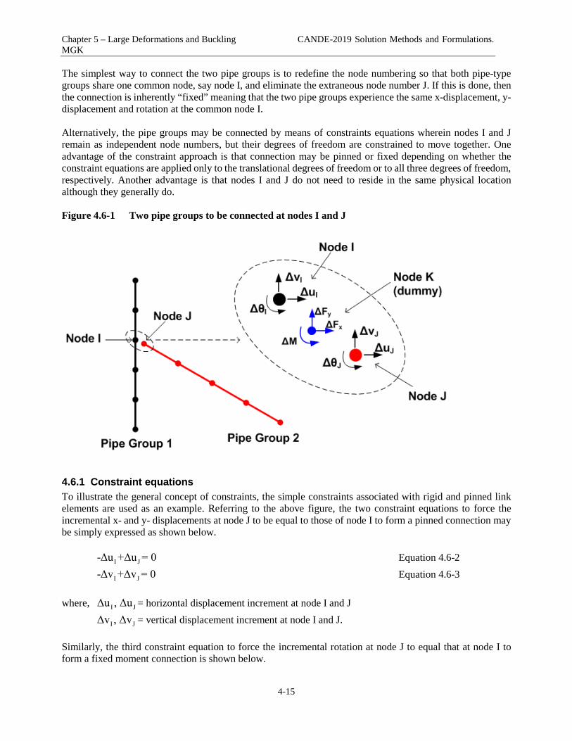
Chapter 5 – Large Deformations and Buckling CANDE-2019 Solution Methods and Formulations. MGK
4-15
The simplest way to connect the two pipe groups is to redefine the node numbering so that both pipe-type groups share one common node, say node I, and eliminate the extraneous node number J. If this is done, then the connection is inherently “fixed” meaning that the two pipe groups experience the same x-displacement, y-displacement and rotation at the common node I. Alternatively, the pipe groups may be connected by means of constraints equations wherein nodes I and J remain as independent node numbers, but their degrees of freedom are constrained to move together. One advantage of the constraint approach is that connection may be pinned or fixed depending on whether the constraint equations are applied only to the translational degrees of freedom or to all three degrees of freedom, respectively. Another advantage is that nodes I and J do not need to reside in the same physical location although they generally do. Figure 4.6-1 Two pipe groups to be connected at nodes I and J
4.6.1 Constraint equations To illustrate the general concept of constraints, the simple constraints associated with rigid and pinned link elements are used as an example. Referring to the above figure, the two constraint equations to force the incremental x- and y- displacements at node J to be equal to those of node I to form a pinned connection may be simply expressed as shown below. I J-Δu +Δu = 0 Equation 4.6-2 I J-Δv +Δv = 0 Equation 4.6-3 where, I JΔu , Δu = horizontal displacement increment at node I and J
I JΔv , Δv = vertical displacement increment at node I and J. Similarly, the third constraint equation to force the incremental rotation at node J to equal that at node I to form a fixed moment connection is shown below.
Chapter 5 – Large Deformations and Buckling CANDE-2019 Solution Methods and Formulations. MGK
4-16
I J-Δθ +Δθ = 0 Equation 4.6-4 where, I JΔθ , Δθ = rotation increment at node I and J. The above constraint equations as well as any set of constraints, can be expressed generally in matrix notation as follows. ˆˆCΔu = 0 Equation 4.6-5 where, C = constraint coefficient matrix ˆΔu = vector of nodal degrees of freedom being constrained 0 = vector of zeroes, one zero for each constraint equation. For example, in the case of the pinned constraints, C is a 2 x 4 rectangular matrix (2 equations x 4 d.o.f.), and for the case of rigid constraints, C is a 3 x 6 rectangular matrix (3 equations x 6 d.o.f). In the general case, Equation 4.6-5 represents any set of constraint equations.
4.6.2 Constraint forces and virtual work Associated with each constraint equation, there exists an unknown internal constraint force enforcing the constraint. For example, the rigid link constraint equations are associated with the following constraint forces (previously illustrated in figure 4.6-1). xΔF = Horizontal force between nodes to maintain I J-Δu +Δu = 0
yΔF = Vertical force between nodes to maintain I J-Δv +Δv = 0
ΔM = Moment required between nodes to maintain I J-Δθ +Δθ = 0 In the above example the constraint forces can be written vector notation as
T
x Yλ = <ΔF , ΔF , ΔM> In preparation for the general virtual work statement, the general constraint equations (Equation 4.6-5) may be expressed in a scalar (work) form as: Tˆ ˆδλ (CΔu) = 0 Equation 4.6-6 where, λ = vector of interface constraint forces, one force component for each constraint. Since ˆδλ is an arbitrary variation of the constraint force vector, Equation 4.6-6 is satisfied if and only if the constraint equations are satisfied. As yet the virtual work of constraint forces has not been established or defined. To this end, we argue that the internal constraint forces produce internal virtual work when the constraint is given a small virtual movement (variation) as follows.

Chapter 5 – Large Deformations and Buckling CANDE-2019 Solution Methods and Formulations. MGK
4-17
T T Tconstraint
ˆ ˆˆ ˆVW = δ(CΔu) Δλ = δu C Δλ Equation 4.6-7 In the above definition for the incremental virtual work of constraints, we assume the system is in equilibrium at load step i and moves to a new equilibrium position at load step i+1 consistent with the incremental constraint equations, which in turn generate incremental constraint forces, Δλ. When the constraints are given a small virtual disturbance (variation), the constraint forces perform virtual work as they move with the virtual disturbance. Physically, this is analogous to imposing constraints with stiff springs between node pairs wherein the internal spring force corresponds to the constraint force. However, in this case the constraint forces are primary unknowns.
4.6.3 Global virtual work statement with constraints With the above understandings, we complete the global formulation by adding the internal virtual work of constraints (Equation 4.6-7) to the standard virtual work statement in Equation 4.6-1 and append the constraint requirement in Equation 4.6-6 to get the general virtual work statement including constraints.
T Tˆ ˆδu Δu ΔPK C - = 0ˆ ˆ 0C 0δλ Δλ
Equation 4.6-8
Since the virtual displacements and virtual constraint forces are arbitrary, the virtual work statement leads to the following global system of equations.
T u PK C
= ˆ 0C 0 λ
∆ ∆ ∆
Equation 4.6-9
The coupled set of global matrix equations is to be solved for nodal displacements and constraint forces. Note that the separate partitioning of the global system into Δu and Δλ is a mere formality and not required in actual global assembly.
4.6.4 General constraint matrix Recalling that the global stiffness equations are formed from the summation element stiffness matrices and load vectors based on each element’s contributions to total virtual work, we can in the same manner construct an element constraint matrix, based on the link element’s contribution to the virtual work as shown below.
T T
e eelink element
ee e
ˆ ˆδu Δu0 CδV = ˆ ˆC 0δλ Δλ
Equation 4.6-10
The above expression represents the contribution of a link element to the global virtual work statement in Equation 4.6-9, therefore, the link element constraint matrix is defined as follows.
T
e
e
0 CC* =
C 0
Equation 4.6-11
where, C* = symmetric link element constraint matrix, dimension (n+m) x (n+m) eC = constraint coefficient matrix for link element, dimension m x n
m = number of constraint equations associated with link element (m = 2 pin, or 3 fix) n = number of constrained degrees of freedom (n= 4 pin, or 6 fix)

Chapter 5 – Large Deformations and Buckling CANDE-2019 Solution Methods and Formulations. MGK
4-18
Equation 4.6-11 is the bottom line result of the virtual work development. That is, C* is the basic link element constraint matrix that needs to be developed for each link type.
4.7 Simple Link Elements The constraint equations for the rigid and pinned links have already been expressed in Section 4.6, therefore all that remains to be done is to develop the constraint element matrix.
4.7.1 Rigid link constraint matrix For the rigid (fixed) link element, all the corresponding degrees of freedom of nodes I and J are constrained to move together. The element’s degrees of freedom and internal forces are aligned in the standard x, y, and θ sequence as shown in the vectors below.
T
e I I I J J J
Te x y
ˆΔu = <Δu ,Δv ,Δθ ,Δu ,Δv ,Δθ >ˆΔλ = <ΔF ,ΔF ,ΔM >
Accordingly, the C* matrix is constructed as shown in the table below based on three constraints. Table 4.7-1 Link element constraint matrix C* for fixed connections
Node I Node J Node K IΔu
IΔv IΔθ JΔu JΔv JΔθ xΔF yΔF ΔM
0 0 0 0 0 0 -1 0 0 0 0 0 0 0 0 0 -1 0 0 0 0 0 0 0 0 0 -1 0 0 0 0 0 0 1 0 0 0 0 0 0 0 0 0 1 0 0 0 0 0 0 0 0 0 1 -1 0 0 1 0 0 0 0 0 0 -1 0 0 1 0 0 0 0 0 0 -1 0 0 1 0 0 0
4.7.2 Pinned link constraint matrix For the pinned connection, the constrained degrees of freedom of nodes I and J are the x and y translations. The element’s degrees of freedom and internal forces are ordered as shown in the vectors below.
T
e I I J J
Te x y
ˆΔu = <Δu ,Δv ,Δu ,Δv >ˆΔλ = <ΔF ,ΔF >
Accordingly, the C* matrix is constructed as shown in the table below based on two constraints. Table 4.7-2 Link element constraint matrix C* for pinned connections
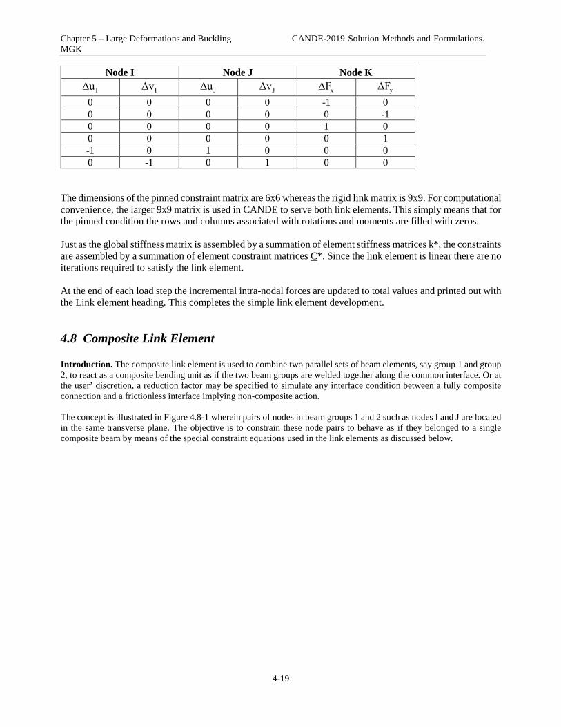
Chapter 5 – Large Deformations and Buckling CANDE-2019 Solution Methods and Formulations. MGK
4-19
Node I Node J Node K IΔu IΔv JΔu JΔv xΔF yΔF
0 0 0 0 -1 0 0 0 0 0 0 -1 0 0 0 0 1 0 0 0 0 0 0 1 -1 0 1 0 0 0 0 -1 0 1 0 0
The dimensions of the pinned constraint matrix are 6x6 whereas the rigid link matrix is 9x9. For computational convenience, the larger 9x9 matrix is used in CANDE to serve both link elements. This simply means that for the pinned condition the rows and columns associated with rotations and moments are filled with zeros. Just as the global stiffness matrix is assembled by a summation of element stiffness matrices k*, the constraints are assembled by a summation of element constraint matrices C*. Since the link element is linear there are no iterations required to satisfy the link element. At the end of each load step the incremental intra-nodal forces are updated to total values and printed out with the Link element heading. This completes the simple link element development.
4.8 Composite Link Element Introduction. The composite link element is used to combine two parallel sets of beam elements, say group 1 and group 2, to react as a composite bending unit as if the two beam groups are welded together along the common interface. Or at the user’ discretion, a reduction factor may be specified to simulate any interface condition between a fully composite connection and a frictionless interface implying non-composite action. The concept is illustrated in Figure 4.8-1 wherein pairs of nodes in beam groups 1 and 2 such as nodes I and J are located in the same transverse plane. The objective is to constrain these node pairs to behave as if they belonged to a single composite beam by means of the special constraint equations used in the link elements as discussed below.

Chapter 5 – Large Deformations and Buckling CANDE-2019 Solution Methods and Formulations. MGK
4-20
Figure 4.8.1. Illustration of beam groups to be joined by composite link elements
4.8.1 Composite constraint equations To develop constraint equations for composite behavior, we consider two beam elements stacked one upon the other representing one element from group 1 and one element from group 2 as shown in Figure 4.8-2. Element 1 is defined with nodes I and L and element 2 is defined with nodes J and M. Each node has three degrees of freedom as shown. Figure 4.8-2 Illustration of two beam elements to be joined as a composite
The axial and transverse displacement functions, as developed in Chapter 2 are shown below in local beam coordinates, x, y1 for element 1 and x, y2 for element 2. (Note that all displacement functions and degrees of freedom are understood to be incremental quantities even though the incremental symbol Δ is not explicitly written)

Chapter 5 – Large Deformations and Buckling CANDE-2019 Solution Methods and Formulations. MGK
4-21
For element 1: 1 1 I 2 L 1 1 1 I 2 I 3 L 4 Lu (x,y) = (φ u + φ u ) + (y - y ) (γ v + γ θ + γ v + γ θ ) ′ ′ ′ ′
1 1 I 2 I 3 L 4 Lv (x) = γ v + γ θ + γ v + γ θ For element 2 2 1 J 2 M 2 2 1 J 2 J 3 M 4 Mu (x,y) = (φ u + φ u ) + (y - y ) (γ v + γ θ + γ v + γ θ ) ′ ′ ′ ′
2 1 J 2 J 3 M 4 Mv (x) = γ v + γ θ + γ v + γ θ where, 1φ (x) = 1 - x/L = Linear interpolation function one.
2φ (x) = x/L = Linear interpolation function two
with, 2 31γ (x) = 1 - 3 (x/L) + 2 (x/L) = Hermitian interpolation function one,
22γ (x) = L (1 - x/L) x/L = Hermitian interpolation function two,
2 33γ (x) = 3 (x/L) - 2 (x/L) = Hermitian interpolation function three,
24γ (x) = L (1 - x/L) (x/L) = Hermitian interpolation function four.
and, 1y = location of neutral axis of element 1, y1 measured from element 1 bottom
2y = location of neutral axis of element 2, y2 measured from element 2 bottom L = element length The first requirement for composite behavior is that the transverse displacement of element 1 is identical to element 2, which is written as, 1 2-v (x) + v (x) = 0 for 0 x L≤ ≤ Inserting the transverse displacement interpolation functions and regrouping nodal degrees of freedom, the above equation may be written as, 1 J I 2 J I 3 M L 4 M Lγ (v -v ) + γ (θ -θ ) + γ (v -v ) + γ (θ -θ ) = 0 . Since the interpolation functions are linearly independent functions of x, the above equation is satisfied if and only if the corresponding degrees of freedom at node pairs are equal, i.e., J I J I M L M L(v -v ) = (θ -θ ) = (v -v ) = (θ -θ ) = 0 Letting node I represent any node in element group 1 and letting node J represent the corresponding node pair in group 2, we can enforce the above constraints for all elements by requiring, I J- v + v = 0 Constraint 1 I J- θ + θ = 0 Constraint 2 where, I & J are all paired nodes along the two beam groups.
Chapter 5 – Large Deformations and Buckling CANDE-2019 Solution Methods and Formulations. MGK
4-22
If we only imposed Constraint Equations 1 and 2 along the parallel beam groups, then the result would be tandem behavior, not composite behavior. By tandem behavior we mean each beam bends about its own neutral axis resulting in relative axial motion (or slippage) at the common interface between beam groups. Consequently, the combined bending stiffness is merely the sum of the two beams. To achieve full composite behavior with enhanced bending stiffness, we must introduce additional constraint equations that preclude relative axial motion at the interface so that planes remain plane over both cross sections. Referring to Figure 4.8-2, the final requirement to achieve composite behavior is obtained by forcing the axial displacement along the top surface of element 1 (y1 = d1) to be equal to the displacement along the bottom surface of element 2 (y2 = 0). This requirement is expressed as, 1 1 1 2 2-u (x, y = d ) + u (x, y = 0) = 0 for 0 x L≤ ≤ Inserting the axial displacement functions and regrouping nodal degrees of freedom this may be written as,
1 J I 2 M L 1 2 J 1 1 I 2 2 J 1 1 I
3 2 M 1 1 L 4 2 M 1 1 L
φ (u -u ) + φ (u -u ) + γ ((y - 0)v - (y - d )v ) + γ ((y - 0)θ - (y - d )θ ) +γ ((y - 0)v - (y - d )v ) + γ ((y - 0)θ - (y - d )θ ) = 0
′ ′′ ′
To simplify the above, we make use of Constraints 1 and 2 by setting J I J I M L M Lv = v , θ = θ , v = v , and θ = θ so that above equation simplifies to the following requirement, 1 J I 2 M L 1 I 2 I 3 L 4 Lφ (u -u ) + φ (u -u ) + h*(γ v + γ θ +γ v + γ θ ) = 0′ ′ ′ ′ where 2 1 1h* = y - y + d After the interpolation functions are inserted in the above expression, we require that the equation remain equal to zero for all values of x, 0 ≤ x ≤ L. Thus the collection of coefficients associated with each power of x (x0, x1, and x2) provides three additional constraint equations that must be enforced as identified below. I J I-u + u + h*θ = 0 (nodes I and J) L M L-u + u + h*θ = 0 (nodes L and M)
I LI L
(θ +θ )-v + v + = 02
L (nodes I and L)
The first two equations are of identical form involving paired nodes from group 1 and group 2, thus we can enforce the first two equations for all elements by requiring, I J I-u + u + h*θ = 0 Constraint 3 where, I & J are all paired nodes between beam group 1 and beam group 2. In contrast to Constraint Equation 3 as well as the previously developed Constraint Equations 1 and 2 involving transverse node pairs I and J, the remaining expression involves longitudinal node pairs I and L associated with beam group 1. We can enforce this last constraint for all elements by requiring,

Chapter 5 – Large Deformations and Buckling CANDE-2019 Solution Methods and Formulations. MGK
4-23
I LI L
(θ +θ )-v + v - L = 02
Constraint 4
where, I & L are the end nodes of each sequential beam element in group 1. To summarize, composite action may be enforced by employing transverse link-type elements between all transverse node pairs I and J to enforce Constraint Equations 1, 2 and 3. In addition, a longitudinal link-type element between all longitudinal node pairs I and L on group 1are required to enforce Constraint Equation 4. Experience has shown that if all beam elements are of uniform length, then Constraint 4 is, in effect, automatically imposed by Constraints 1, 2. Thus for those parallel beam groups where all elements have the same length L, only the transverse constraints need to be defined in the CANDE model. For the more general case, both the transverse and longitudinal constraints need to be defined in the CANDE model.
4.8.2 Composite constraint forces Associated with each of the four constraint equations, there is a corresponding constraint force that maintains the kinematic constraint. Listed below is a summary of the four constraint equations along with the associated constraint force. The constraint forces are unknowns that are determined by CANDE during the course of the solution. From this point on in the development, the asterisk symbol (*) is introduced to explicitly denote all quantities that are expressed in local beam coordinates, x* implying the axial direction and y* the transverse direction. Also the delta symbol (Δ) is introduced to remind us that the quantities are incremental solution values at each load step. Constraints and forces for transverse link element (I and J nodes):
1. Transverse displacements. This constraint forces the transverse displacement at node I in group 1 to equal the transverse displacement at node J of group 2.
I J-Δv * + Δv * = 0
The associated constraint force is the transverse force ΔFy* required to hold the beams together in the transverse direction. ΔFy* is a solved-for variable contained in the dummy node K of the link element.
2. Rotations. This constraint forces the rotation at node I in group1 equal to the rotation of node J in group 2.
I J-Δθ + Δθ = 0 The associated constraint moment ΔM is the moment required to enforce equal rotations at the I-J cross section. ΔM is a solved-for variable contained in the dummy node K.
3. Axial displacements. This constraint insures planes remain plane across both beam groups by forcing the axial
displacements at each beam centerline to form a straight line with the common rotation angle IΔθ , which is
equivalently expressed as I J(Δθ +Δθ )/2 because the rotations at nodes I and J are equal. Thus the constraint is written as,
I J I J-Δu* + Δu* + h*(Δθ +Δθ )/2 = 0
where, 2 1 1h* = y - y + d , is the distance between beam centroids.

Chapter 5 – Large Deformations and Buckling CANDE-2019 Solution Methods and Formulations. MGK
4-24
The associated constraint force is the longitudinal shear force ΔFx* required to hold the beams from slipping in shear along surface between the two beam groups. ΔFx* is a solved-for variable contained in the dummy node K. Reduced shear connection. The shear force ΔFx* is directly proportional to h*. Therefore in order to simulate a reduced shear connection we introduce a user-specified reduction factor ρ to reduce h* to ρh*, where 0 ≤ ρ ≤ 1. If the user chooses ρ = 1, a fully composite is section modeled with a perfect shear connection. For ρ = 0.5 the shear connection is assumed to be 50% effective, and for ρ = 0 the shear connection is completely absent (greased interface) and the two beams behave in tandem with additive bending stiffness.
Constraints and forces for longitudinal link element (I and L nodes):
4. Longitudinal constraint. This constraint insures that the difference in the transverse displacement at the ends of each beam is equal to the average beam slope times the element length.
I LI L
(Δθ +Δθ )-Δv * + Δv* - L = 02
If all the beam elements in both groups are assigned the same element length L, then this constraint is automatically satisfied at all interior nodes of the group by constraints 1 and 2. Thus this constraint need not be enforced if the elements are all the same length with the consequence of a small error (generally less than 5%) in the moment prediction at end nodes of each beam group.
The associated constraint force is the vertical shear force ΔFy* due to the bending gradient across the composite-element pair. Consequently, the shear force does not appear in the standard element printout, but rather it appears in the constraint force printout. The user must be aware of this strange consequence in assessing the structural responses of the composite beam groups. In general it is recommended to define the CANDE model with uniform beam element lengths and ignore the longitudinal constraint elements.
4.8.3 Constraint global-local transformations To assemble the constraints into the composite link element matrices, the local degrees of freedom need be expressed in global degrees of freedom using the coordinate transformation angle φ as illustrated in the figure below.

Chapter 5 – Large Deformations and Buckling CANDE-2019 Solution Methods and Formulations. MGK
4-25
Figure 4.8-3. Local and global coordinates of composite beam elements.
The transformation equations are written as follows.
Δu* = cosφΔu + sinφΔvΔv* = -sinφΔu + cosφΔv
* = θ θ∆ ∆
Note there is no need to transform the constraint forces and moments to global values because these are stand-alone quantities in the system matrix associated with dummy K nodes that are not shared with any other elements.
4.8.4 Transverse-link constraint matrix The transverse-composite link constraint equations, expressed in global degrees of freedom, are listed below beginning with the 3rd constraint listed above.
1. Axial displacement constraint in global coordinates.
I I J J I I-cosφΔu -sinφΔv +cosφΔu +sinφΔv +ρh*(Δθ +Δθ )/2 = 0 2. Transverse displacement constraint in global coordinates.
I I J J sinφΔu -cosφΔv -sinφΔu +cosφΔv = 0
3. Rotation constraints (same in x,y and x*,y* systems)
I J-Δθ + Δθ = 0 Following the previous virtual work development for constraint equations and constraint forces, the constraint matrix for the transverse-composite link element is established as shown in the matrix-table below.

Chapter 5 – Large Deformations and Buckling CANDE-2019 Solution Methods and Formulations. MGK
4-26
Table 4.8-1. Composite-transverse link element matrix (CANDE code 10) Node I Node J Node K
IΔu
IΔv IΔθ JΔu JΔv JΔθ xΔF* yΔF* ΔM
0 0 0 0 0 0 -c s 0 0 0 0 0 0 0 -s -c 0 0 0 0 0 0 0 ρh*/2 0 -1 0 0 0 0 0 0 c -s 0 0 0 0 0 0 0 s c 0 0 0 0 0 0 0 ρh*/2 0 1 -c -s ρh*/2 c s ρh*/2 0 0 0 s -c 0 -s c 0 0 0 0 0 0 -1 0 0 1 0 0 0
Where ρ is the user specified fraction of composite action desired, and h* is the computed distance between the neutral axis at node I and the neutral axis at node J.
4.8.5 Longitudinal-link constraint matrix The longitudinal-composite link consists of just one constraint equation and is expressed in global degrees of freedom as,
I LI I L L
(Δθ +Δθ )sinφΔu -cosφΔv -sinφΔu +cosφΔv - L = 02
The corresponding matrix for the longitudinal-composite link element is shown in the matrix below, Table 4.8-2. Material Properties. The composite link elements require “material property” input data to define the two beam groups for which at least a portion of their lengths are being combined into composite action. Also, the material data defines the desired fraction of composite action (0 to 1.0) To this end, Material Type #7 has been introduced into the CANDE-2019 program for input on line D-1 along with the material number assigned to the composite link element first defined on input-line C-4 (the independent material numbers may range from 1 to 30). Input-line D-2 defines the two beam group numbers being combined as well as the fraction of composite action. This information is printed out in the CANDE report under the material property heading. Table 4.8-2. Composite-longitudinal link element matrix C* (CANDE code 11)
Node I Node L Node N
IΔu
IΔv IΔθ JΔu JΔv JΔθ xΔF * yΔF * ΔM
0 0 0 0 0 0 0 s 0 0 0 0 0 0 0 0 -c 0 0 0 0 0 0 0 0 -L/2 0 0 0 0 0 0 0 0 -s 0 0 0 0 0 0 0 0 c 0 0 0 0 0 0 0 0 -L/2 0 0 0 0 0 0 0 0 0 0 s -c -L/2 -s c -L/2 0 0 0 0 0 0 0 0 0 0 0 0
Where L is beam length between nodes I and L, and node N is a dummy node.

Chapter 5 – Large Deformations and Buckling CANDE-2019 Solution Methods and Formulations. MGK
4-27
4.9 Link Element Death The link element death option has many practical applications such as removing temporary construction bracing, creating void openings in soil zones, and simulating the deterioration of structural segments as illustrated in the MGK CANDE-2019 User manual. The life and death of link elements are measured by the load-step counter, IA = 1, 2, 3 … NINC, where NINC is the maximum number of load steps to be executed in a given problem. There are two key load-step numbers assigned to each link element by the user as defined below,
1. IAC = load-step number when link element enters the system (birth)
2. IAX = load-step number when link element is removed from system (death) Where, it is required that IAC < IAX so that the element is born before it dies.
4.9.1 Procedure for element death Assuming the link element entered the system (born) at load-step number IA= IAC, then element death will be initiated when IA = IAX. Initiation of element death requires the following changes to the solution algorithm, 1. When IA = IAX, bypass the construction of the constraint matrix and skip the global assembly of the constraint matrix. 2. Create a link-element load vector containing the negative values of the element’s accumulated constraint forces through load step IAX-1. To illustrate, the negative load vector for a rigid link is shown below (9 components).
T
X Yf = < 0, 0, 0, 0, 0, 0,-F *,-F *,-M*> 3. Assemble the link element load vector into the global load vector and solve the global system as usual.
4. After the successful solution of load-step IA = IAX, the link element is no longer part of the system, the link-element’s constraint forces are redistributed to the system, and the element’s accumulated constraint forces are equal to zero. 5. For all load steps IA > IAX, the procedure is to simply bypass all operations with the constraint matrix and load vector associated with the dead link element. As a side comment, it is noted that there is no theoretical problem in developing a similar death-element option for beam elements and continuum elements directly. However, the link-element has the special advantage that the accumulated constraint forces are already available in computer storage facilitating the construction of the negative load vector.
4.9.2 Programming strategy Initial storage for the new variable IAX is logically resolved as an addition to the element property vector, IX. Specifically, the vector is extended from IX(7) to IX(8) as indicated by the data input line C-4 in Chapter 4. This extension requires corresponding extensions in two other storage matrices as follows. In subroutine GENEL the element property array NOD(7, Numel) is expanded to NOD(8,Numel) to store the IX(8) value. Similarly in subroutine HEROIC the array MNO(3,Numel) is expanded to MNO(4,Numel) for the same purpose. The subroutines that required changing under the element death option for the link element are:
• GENEL – minor changes for printing out in CANDE report. • STIFNS – minor change in call to subroutine XLINK with more variables. • XLINK – significant changes reflecting all link element developments. • RESOUT – Improved output of link element including status (alive or dead)

Chapter 5 – Large Deformations and Buckling CANDE-2019 Solution Methods and Formulations. MGK
5-28
LARGE DEFORMATIONS AND BUCKLING This chapter presents the development of beam theory with large deformations that includes beam bending, column deformation, material nonlinearity, and incremental loading. The development is an extension on the small-deformation beam theory presented in Section 2.1 but removes the limitations of small deformation theory.
5.1 Updated Lagrange Formulation The major assumptions and limitations are listed below:
1. Two-dimensional framework in a plane strain formulation. 2. Bernoulli-Euler beam kinematics without shear deformation. 3. Material nonlinearity is a function of normal stress and strain. 4. Incremental virtual work formulation with incremental stress-strain relationships and loading. 5. Updated Lagrange strain-displacement relationship appropriate for large rotations and small stretch.
5.1.1 Coordinates and incremental relationships. Consider a beam element originally in an undeformed state that has experienced a sequence of load steps (1, 2, 3, …i) and is in equilibrium after load step i. Let the nodes at either end of the element be labeled “a” and “b”, and let their current location in the global X-Y coordinate system be denoted as (Xai, Yai) and (Xbi, Ybi), respectively. Next, construct a local x-y coordinate system with the origin at node a. The x-axis extends from node a to node b along the base of the beam, and the y-axis is orthogonal to the x-axis with y = 0 at the bottom of the beam cross section. From this reference position we apply load step i + 1 and seek to determine the incremental structural responses. The local displacement increments in displacing from load step i to step i + 1 will be denoted as Δu in the x direction and Δv in the y direction. Equilibrium of all the forces and moments acting on the element at load step i + 1 will be in reference to the x-y coordinate system of the previous load step i, not the element’s original position as assumed in small deformation theory.
5.1.2 Bernoulli-Euler beam kinematics. Based on the assumption that cross-sectional planes remain plane in bending and axial deformation, the well-known Bernoulli-Euler assumption for displacement increments Δu and Δv at any station x along the beam length and at any point y in the beam’s cross section may be expressed as: Δu(x, y) = Δa(x) + (y*-y)Δv’ Equation 5-1 Δv(x) = Δv(x) à a function of x only Equation 5-2 where, Δu(x,y) = displacement in x direction from column and bending deformation
Δa(x) = uniform displacement in x direction from column, independent of y Δv(x) = displacement in y direction as function of x, independent of y Δv’ = d(Δv)/dx, derivative of Δv with respect to x (local deformation slope) y* = a reference plane in the beam cross section at y = y*, yet to be specified ( )’ = d( )/dx, prime symbol denotes derivative of any quantity with respect to x
5.1.3 Total Lagrangian strain for large rotations. The total normal strain (x direction) at load step i at any station x along the beam length and at any point y in the beam’s cross section may be described by a truncated form of total Lagrangian strain given by, Ε i(x,y) = ui ’ + ½(vi’)2 Equation 5-3a

Chapter 5 – Large Deformations and Buckling CANDE-2019 Solution Methods and Formulations. MGK
5-29
All quantities are in reference to the original undeformed position, i = 0. It is evident that ui’ is the standard definition of small strain in the x direction. The nonlinear term, ½(vi’)2, is a second order correction term that adds a uniform stretching strain to the axial strain as a result of beam rotation. The correction term may be visualized as the stretch that is induced in the leg of a right triangle as it is rotated into the position of the hypotenuse through an angle approximated by vi ’. The larger the value of vi’ the more inaccurate is the approximation of the angle. If we express an increment of the total Lagrangian strain from step i to i+1 we obtain: ΔΕ(x,y) = Ε i+1(x,y) - Ε i(x,y) = Δu’ + ½( Δv’)2 + vi’Δv’ Equation 5-3b The last term in Equation 5-3b contains vi’, which is not an incremental term but rather the approximated angle at step i in reference to the undeformed position at i = 0. Thus the incremental form of total Lagrangian strain, ΔΕ (x,y), produces the same error as Equation 5-3a when dealing with large rotations. Note that when determining the strain increment for the first load increment starting from i = 0, we have vi’ = v0’ = 0, because the reference configuration has no displacements or rotations.
5.1.4 Updated Lagrangian strain increments. The so-called updated Lagrange formulation provides improved accuracy for calculating strains by updating the x and y coordinates of the beam element’s position to step i prior to solving for step i + 1. In other words the beam element’s position at step i is taken as the reference position for equilibrium and for measuring additional displacements resulting from the loads that are imposed at step i + 1, which means vi’ = 0 for each load step from i to i + 1. With the above understanding, we can rewrite Equation B-3 in the updated Lagrangian description as: Δε (x,y) = Δu’ + ½( Δv’)2 Equation 5-4a where the symbol Δε is used to represent updated Lagrangian strain increments in order to distinguish it from increments of total Lagrangian strain, ΔΕ. Inserting the Bernoulli-Euler kinematical equations for Δu into the updated Lagrangian strain increment equation, we arrive at the incremental strain-displacement relationships for beams under large rotations, given as, Δε(x,y) = Δa’+ (y*-y) Δv’’+ ½(Δv’)2 Equation 5-4b Equation 5-4b is the new equation for this development. That is, the remainder of the basic equations for the nonlinear stress-strain model, internal force resultants, and virtual work remain valid as expressed in the small-deformation formulation. However, the interaction of these basic equations with Equation 5-4b results in new nonlinear governing equations for beam deformations.
5.1.5 Incremental stress-strain model. The nonlinear stress-strain laws used in CANDE are specific to each pipe material such as corrugated metal and reinforced concrete, which are detailed in previous chapters. However, all these stress-strain models conform to the same generic form that may be expressed as Δσ = Ec Δε Equation 5-5 where, Δσ = increment of axial stress from load step i to i + 1, (Δσ = Δσ (x,y)) Δε = increment of axial strain from load step i to i + 1, (Δε = Equation 5-4b) Ec = chord modulus of total stress-strain curve from load step i to i + 1

Chapter 5 – Large Deformations and Buckling CANDE-2019 Solution Methods and Formulations. MGK
5-30
The chord modulus is dependent on the pipe material and the history of stress and strain throughout all loading steps. It is determined iteratively during each load step by repeating the solution process until the value of Ec converges for each element to a small tolerance of error. Replacing Δε in Equation 5-5 with Equation 5-4b, the fundamental stress-displacement relationship may be expressed as, Δσ = Ec(Δa’+ (y*-y) Δv’’+ ½(Δv’)2) Equation 5-6 Next, we will use Equation 5-6 to define the internal thrust and internal moment acting on the cross section at any station x.
5.1.6 Internal thrust and moment increments. As is customary, we define the thrust increment as the integral of Δσ over the cross section area A, and the moment increment as the integral of Δσ (y*-y) over the cross section area A. Specifically,
ΔN = ∫A Δσ dA = ∫A Ec(Δa’+ (y*-y) Δv’’+ ½(Δv’)2) dA Equation 5-7a ΔM = ∫A Δσ (y*-y) dA = ∫A Ec(Δa’+ (y*-y) Δv’’+ ½(Δv’)2) (y*-y) dA Equation 5-7b where, ΔN = thrust increment from load step i to i + 1, (ΔN = ΔN (x)) ΔM = moment increment from load step i to i + 1, (ΔM = ΔM (x)) dA = b(y)dy, a differential area of cross section where b(y) is the width with y measured from bottom. The arbitrary reference position y* is now chosen so that ∫A Ec (y*-y) dA = 0, which simplifies Equations 5-7a,b, and gives the location of y* measured from the bottom as, y* = ( ∫A Ec y dA) / (∫A Ec dA) Equation 5-8 The remaining area integrals in Equation 5-7a,b relate to effective axial stiffness and effective bending stiffness and are defined as, EA* = ∫A Ec dA = Effective axial stiffness of beam element Equation 5-9 EI* = ∫A Ec (y*-y)2dA = Effective bending stiffness of beam element Equation 5-10 All of the integrals in Equations 5-8, 5-9, and 5-10 are computed numerically for every iteration within each load step until convergence is achieved. With the above definitions for y*, EA* and EI*, the thrust and moment increments (Equations 5-7a,b) simplify to the following equations, ΔN = EA*(Δa’ + ½(Δv’)2) Equation 5-11 ΔM = EI* Δv’’ Equation 5-12 Note that the moment-increment expression is the familiar bending stiffness-curvature relationship used in small deformation theory. However, the thrust-increment expression, in addition to the familiar column stiffness-deformation relationship, also contains a nonlinear stiffness term related to rotation, ½(Δv’)2.
5.1.7 Virtual work for beam-column element. The general concept of virtual work is fully developed in Chapters 1 and 2. Here the attention is focused on the internal virtual of beam-column elements.

Chapter 5 – Large Deformations and Buckling CANDE-2019 Solution Methods and Formulations. MGK
5-31
The internal virtual work for the beam-column element under consideration may be expressed as the following volume integration at any load step i + 1: δU i+1 = ∫V δε i+1σ i+1 dV Equation 5-13 where, δε i+1 = virtual strain field arising from the imposed virtual displacements σ i+1 = stress field existing in beam element at load step i +1
∫V (…) dV = volume integration over the beam element The virtual symbol δ means a small variation of the strain field. Similar to variational calculus, δ operates on the displacement variables like a total derivative. Thus operating on the updated Lagrangian strain, the virtual strain field is determined as: δε i+1 = δ[a’ + (y*-y) v’’ + ½(v’)2] i+1 = δa’ + (y*-y)δv’’ + v’ i+1δv’ Equation 5-14 The displacement variables prefaced with the symbol δ are arbitrary motions and need not be associated with the values at load step i+1. However, the term v’ i+1 is associated with load step i+1 and is equivalent to, v’ i+1 = Δv’, since v’ i = 0 by virtue of the updated Lagrange formulation. The incremental form of the element internal virtual work is defined by; δΔUe = δU i+1 - δU i = ∫V (δε i+1σ i+1 – δε i σ i )dV Equation 5-15 Observing that δε i+1= δε i + Δv’δv’, the above becomes; δΔUe = ∫V {(δa’+(y*-y)δv’’)Δσ + Δv’δv’σ i+1 }dV Equation 5-16 Separating the volume integral into area and length integrals, dV = dAdx, we arrive at,
δΔUe = ∫x{δa’ ∫AΔσ dA + δv’Δv’ ∫Aσ i+1 dA + δv’’ ∫AΔσ (y*-y)dA} dx Equation 5-17 Here it is observed that the two area integrals involving Δσ have already been identified as ΔN and ΔM in Equations 5-7a,b. The area integral involving σ i+1 will now be designated as Ni+1, which is the total thrust at step i+1 referred to the beam element’s coordinate system at step i. Thus Equation 5-17 is written as; δΔUe = ∫x{ δa’ΔN + δv’ Δv’ Ni+1 + δv’’ΔM } dx Equation 5-18 Since we have already established expressions for ΔN and ΔM in terms of displacements in Equations 5-11 and 5-12, we replace the unknown force increments ΔN and ΔM in Equation 5-18 with the equivalent unknown displacements. However with regard to Ni+1, which is nonlinear because it is coupled with Δv’, we choose to leave Ni+1 as expressed to facilitate the nonlinear solution strategy. With the above replacements, Equation 5-18 becomes,
δΔUe = ∫x{δa’EA*Δa’ + δa’EA* ½(Δv’)2 + δv’Δv’Ni+1 + δv’’EI*Δv’’} dx Equation 5-19 For the sake of clarity, we will express Equation 5-19 as the sum of four terms,
δΔUe = δΔUa + δΔUr + δΔUg + δΔUb Equation 5-20 where, δΔUa = ∫x{δa’EA*Δa’} dx Equation 5-20a δΔUr = ∫x{δa’EA* ½(Δv’)2}dx Equation 5-20b

Chapter 5 – Large Deformations and Buckling CANDE-2019 Solution Methods and Formulations. MGK
5-32
δΔUg = ∫x{δv’Δv’ Ni+1 }dx Equation 5-20c δΔUb = ∫x{δv’’EI*Δv’’}dx Equation 5-20d Of the four terms in Equation 5- 20, the first term is the familiar column stiffness term and the fourth term is familiar bending stiffness term identical to small deformation theory. The middle two terms are nonlinear and are associated with large deformations. As we shall see in the subsequent FEM development, the second term will be treated as a load vector and the third term will lead to the so-called geometric stiffness matrix.
5.2 Finite Element Development
5.2.1 Finite element interpolation functions. Equation 5-20 is the incremental internal virtual work of a beam column element with large deformation without numerical approximations. To express this in a FEM formulation we introduce interpolation functions for the displacements that become exact as the element lengths become small. The interpolation functions are expressed in terms of unknown nodal variables shown in the sketch below.
L = length where, Δua, Δub = incremental nodal displacements in x direction at nodes a and b Δva, Δvb = incremental nodal displacements in y direction at nodes a and b Δθa, Δθb = incremental nodal rotations in counter-clockwise direction at nodes a and b The incremental axial displacement function is approximated with a linear interpolation function expressed in vector notation as;
Δa(x) = < φ1 φ2 > < Δua Δub>T Equation 5-21 where, φ1(x) = 1 – x/L φ2(x) = x/L L = element length The incremental vertical displacement function is approximated by a cubic polynomial, known as a Hermitian interpolation function, and is expressed in vector notation by, Δv(x) = < γ1 γ2 γ3 γ4 > < Δva Δθa Δvb Δθb>T Equation 5-22
where, γ1(x) = 1 – 3 (x/L)2 + 2 (x/L)3 γ2(x) = L (1 – x/L)2 x/L
γ3(x) = 3 (x/L)2 – 2 (x/L)3 γ4(x) = L (1 – x/L) (x/L) 2
Node b
ua ub θa θb
Node a
( )
vb va
x
y
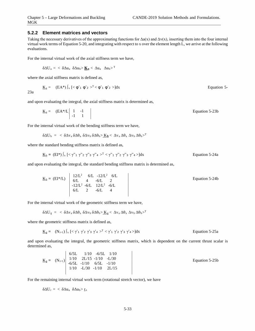
Chapter 5 – Large Deformations and Buckling CANDE-2019 Solution Methods and Formulations. MGK
5-33
5.2.2 Element matrices and vectors Taking the necessary derivatives of the approximating functions for Δa(x) and Δv(x), inserting them into the four internal virtual work terms of Equation 5-20, and integrating with respect to x over the element length L, we arrive at the following evaluations. For the internal virtual work of the axial stiffness term we have, δΔUa = < δΔua δΔub> Ka < Δua Δub> T where the axial stiffness matrix is defined as, Ka = (EA*) ∫x [< φ’1 φ’2 >T < φ’1 φ’2 >]dx Equation 5-23a and upon evaluating the integral, the axial stiffness matrix is determined as, Ka = (EA*/L) Equation 5-23b For the internal virtual work of the bending stiffness term we have, δΔUb = < δΔva δΔθa δΔvb δΔθb> Kb < Δva Δθa Δvb Δθb>T
where the standard bending stiffness matrix is defined as, Kb = (EI*) ∫x [< γ’’1 γ’’2 γ’’3 γ’’4 >T < γ’’1 γ’’2 γ’’3 γ’’4 >]dx Equation 5-24a and upon evaluating the integral, the standard bending stiffness matrix is determined as, Kb = (EI*/L) Equation 5-24b For the internal virtual work of the geometric stiffness term we have, δΔUg = < δΔva δΔθa δΔvb δΔθb> Kg
< Δva Δθa Δvb Δθb>T where the geometric stiffness matrix is defined as, Kg = (Ni+1) ∫x [< γ’1 γ’2 γ’3 γ’4 >T < γ’1 γ’2 γ’3 γ’4 >]dx Equation 5-25a and upon evaluating the integral, the geometric stiffness matrix, which is dependent on the current thrust scalar is determined as, Kg = (Ni+1) Equation 5-25b For the remaining internal virtual work term (rotational stretch vector), we have δΔUr = < δΔua δΔub> re
1 -1 -1 1
12/L2 6/L -12/L2 6/L 6/L 4 -6/L 2 -12/L2 -6/L 12/L2 -6/L 6/L 2 -6/L 4
6/5L 1/10 -6/5L 1/10 1/10 2L/15 -1/10 -L/30 -6/5L -1/10 6/5L -1/10 1/10 -L/30 -1/10 2L/15

Chapter 5 – Large Deformations and Buckling CANDE-2019 Solution Methods and Formulations. MGK
5-34
wherein the rotational stretch vector is expressed as, re = ρ (EA*/2L) <-1 1>T Equation 5-26a where, ρ = ∫x (Δv’)2dx = < Δva Δθa Δvb Δθb> Kg* < Δva Δθa Δvb Δθb>T Kg* = Kg without the multiplier (Ni+1)
Thus, the rotational stretch vector, which is dependent on the nonlinear scalar ρ, is determined as, re = = ρ (EA*/2L) Equation 5-26b The above four terms of the element’s internal virtual work, δΔUe, may be brought together into a single 6 x 6 matrix along with 6-component vectors where the six nodal unknowns are listed in the following order < Δua Δva Δθa Δub Δvb Δθb>. Thus the finite element equivalent of Equation 5-20 is expressed as, δΔUe = < δ Δua δΔva δΔθa δΔub δΔvb δΔθb> ( Ke < Δua Δva Δθa Δub Δvb Δθb> T + re ) where, Ke = total effective element stiffness matrix (6 x 6) Equation 5-27 re = < ra 0 0 rb 0 0 >T = rotational stretch vector (1 x 6) Equation 5-28 Of course, it is understood that the components of Ka, Kb, and Kg are added into the proper locations of the Ke matrix corresponding to the ordering of nodal variables.
5.2.3 Transformation and global assembly. The last step before adding the element’s contribution of δΔUe into the entire system is to transform the nodal variables from local coordinates to global coordinates. Let β = angle from global X-axis to local x-axis, then the local nodal variables may be expressed as global nodal variables by, Δue = T ΔuE Equation 5-29
where, Δue = < Δua Δva Δθa Δub Δvb Δθb> T local nodal variables for element ΔuE = < ΔuA ΔvA ΔθA ΔuB ΔvB ΔθB> T global nodal variables for element T = and, C = cos(β) and S = sin(β) With the above transformation matrix, the element stiffness matrix and rotational stretch vector may be expressed in global coordinates as,
-1 1
ra rb
C S 0 0 0 0 -S C 0 0 0 0 0 0 1 0 0 0 0 0 0 C S 0 0 0 0 -S C 0 0 0 0 0 0 1

Chapter 5 – Large Deformations and Buckling CANDE-2019 Solution Methods and Formulations. MGK
5-35
KE = TT Ke T Equation 5-30 rE = TT re Equation 5-31 It should be clear that lower-case subscripts are used for element quantities that are in expressed in local coordinates, whereas upper-case subscripts are used for element quantities that are in expressed in global coordinates. The effevtive element stiffness matrix KE and the rotational stretch vector rE are in the proper form for global assembly wherein KE is added to the global effective stiffness matrix and rE is brought to the right-hand-side of the equations to be subtracted from the load vector.
5.3 Solution Strategy The overall solution process is a direct iterative method as outlined below. The viewpoint is that we have a converged solution at load step i, and we seek a solution for load step i+1.
5.3.1 Iterative methodology In obtaining a solution from load step i to i+1, we begin by assuming Ni+1 = Ni and ρ = 0 so that element matrices and vectors may be computed for each element. After global assembly, the current set of equations may be expressed for iteration k as KGk ΔuGk = ΔPGk Equation 5-32 where, KGk = global stiffness matrix for iteration k, i.e., collection of elements ∑ KEk ΔuGk = global vector of all unkown nodal variiable increments for iteration k ΔPGk = global vector of load increments for iteration k, including negative rotational-stretch vector. k = iteration counter; 1, 2, 3, … The set of linear alebraic equations represented by Equation 5-32 is solved by Gauss Elimination for the dispacement increments ΔuGk. This trial solution is used to form a new and better estimates for Ni+1 and ρ, which leads to revised values for KGk and ΔPGk for the next iteration. When two successive iterations produce the same results within an acceptable tolerance, the solution has coverged for load step i + 1, and all quantities are updateded as, q i+1 = q i + Δq Equation 5-33 where q stands for all structural responses such as displacements, stresses, strains, moments, thrusts, and so on. In addition, the updated Lagrange formulation implies that the global coordinate locations of each node are updated so that q also repesents each (X,Y) nodal coordinate that are updated by the corresponding displacement increments.
5.3.2 Recovery of element forces When load step i+1 converges to a solution, we want to recover the incremental internal forces at the ends of the element, that is, increments of thrust, shear and moment at the element’s nodes. We can obtain these force increments in reference to “configuration i coordinates” by making use of virtual work. Let, ΔTa, ΔTb = Thrust force increments (xi direction) at nodes a and b ΔQa, ΔQb = Shear force increments (yi direction) at nodes a and b ΔMa, ΔMb = Moment increments at nodes a and b (invariant to x-y coordinates)

Chapter 5 – Large Deformations and Buckling CANDE-2019 Solution Methods and Formulations. MGK
5-36
The incremental virtual external work of these end forces is given by; δΔWe = < δ Δua δΔva δΔθa δΔub δΔvb δΔθb> < ΔTa ΔQa ΔMa ΔTb ΔQb ΔMb>T
With the element’s incremental end loads defined, we can now express the net incremental virtual work of any element to be equal to zero; i.e., δΔVe = δΔUe - δΔWe = 0 Using equation Equations 5-27 and 5-28 to express δΔUe, we arrive at the following equations to determine the incremental end forces and moments:
a a a
a a
a a
b b b
b b
b b
a b g
ΔT Δu r
ΔQ Δv 0
ΔM Δθ 0+
ΔT Δu r
ΔQ Δv 0
ΔM Δθ 0
+ +=
K K K
Equation 5-34
Thus the end forces can be recovered by multiplying the complete element stiffness matrix times the incremental displacements. For the end thrust forces we also add on the rotational stretch forces ra and rb . All of the above operations are carried out in reference to local the coordinate axis at step i.
5.3.3 Update coordinates Before proceeding to the next load step, it is neccessary to update all quatities to the new starting configuation. In particular we need to update the thrust associated with the geometric stiffness matrix. Let N* represent the accumulation of all past thrust increments which is expressed in the x-direction of the previous step (i,e., N* = Ni+1). Similary let Q* represent the accumulation of all past shear increments which is expressed in the y-direction of the previous step The goal is to express in N* in the x-direction and Q* in the y-direction of the current position. The increment of rotation, say α, that the element experienced in moving from the previous step to the current step may be computed as: Lnew = (Lold+ Δub - Δua)2 + (vb –va)2)1/2 (new length of element) Equation 5-35a sinα = (vb –va)/ Lnew Equation 5-35b cosα = (Lold + Δub - Δua)/ Lnew Equation 5-35c Thus we can rotate the thrust and shear to the current configuration as N*α = cosα N* + sinα Q* Equation 5-36a Q*α = -sinα N* + cosα Q* Equation 5-36b For the iteration process during the next load step, we use the following estimate for thrust in the geometric stiffness matrix; Ni+1 = N*α + ΔN Equation 5-37

Chapter 5 – Large Deformations and Buckling CANDE-2019 Solution Methods and Formulations. MGK
5-37
where N*α is a fixed value and ΔN is determined iteratively. For the first iteration we assume ΔN = 0. In the absence of material nonlinearity, this process always converges in three load steps. After all load steps are complete, the problem is finished and the load-deformation path of the structural system may be visualized. Note that this method of analysis by itself does not directly provide a critical buckling load like a linearized buckling (Euler) analysis. Rather, the actual buckling load is observed by noting the peak load (e.g., soil height) when the system fails due to unbounded displacements. In order to predict the buckling capacity at the end of each load increment, we augment the large-deformation analysis with a linearized buckling solution as discussed next.
5.4 Buckling Capacity At the end of each converged load step, we have stored in memory the current components for the standard stiffness matrix and the geometric stiffness matrix, which, when taken together, form the global stiffness matrix that is expressed in Equation 5-32. Thus after convergence of load step i+1, we may write the global stiffness matrix in two parts as, KG = KS + KGeo(Ni+1) Equation 5-38 where, KS = global standard stiffness matrix (small deformations) KGeo(Ni+1) = global geometric stiffnes matrix written as a function of element thrust values The known values for thrust Ni+1 as expressed in the above geometric stiffness matrix, have been determined iteratively during the solution for step i + 1. Thus, Ni+1 represents the current set of thrust values in the various beam-column elements at load step i+1. If we temporarily assumed the matrices in Equation 5-38 remain constant except the geometric stiffness is scaled by a load parameter “c”, then we can determine what magnitude increase in the set of thrust values Ni+1 that would cause unlimited deformations, i.e., critical buckling. This will occur when the combined standard and geometric stiffness becomes singular (determinant = 0), which is dependent on the value of c. To this end, let the global stiffness matrix be written as,
KG(c) = KS + c KGeo(Ni+1) Equation 5-39 and pose the problem as, find the value(s) c such that, Det KG(c) = 0 Equation 5-40 This, of course, is the classic eigenvalue problem for buckling bifurcation wherein the lowest eigenvalue “c” is a direct measure of the current buckling capacity. If, for example, the value of c is found to be 2.50, then the current set of thrust values Ni+1 could be increased by any factor up to 2.5 before buckling would occur. Thus we can say that the value of “c” is the predicted buckling capacity or equivalently the safety factor against buckling. In CANDE-2019, a determinant search process finds the value of “c”. Starting with the guess c = 1, the determinant expressed in Equation 5-40 is evaluated. If the determinant is positive, meaning the matrix is structurally stable, then the value of c is steadily increased until the determinant is found to be negative, meaning the matrix structurally unstable. Knowing the correct value c lies in an interval bounded by the last two estimates, a binary-chop method is used to keep refining the estimate for “c” until it is accurate to two decimal places. In summary, this chapter presents a complete derivation of a beam theory with large deformations that includes beam bending, column deformation, material nonlinearity, and incremental loading. The large deformation responses (forces, displacements, stresses and strain) are output at the end of each load step along with a prediction of the buckling capacity.

Chapter 5 – Large Deformations and Buckling CANDE-2019 Solution Methods and Formulations. MGK
5-38
5.5 Illustration – Simply Supported Beam This illustration compares the updated Lagrange CANDE-2019 solution and buckling prediction with a closed-form solution for an axially load, simply supported beam with initial constant end moment. The closed-form solution is theoretically equivalent to a one-step updated Lagrange solution (i.e., total Lagrange method) so that a direct comparison may be made if we limit the CANDE solutions to a single load step. Subsequently, we will obtain CANDE solutions with multiple load-steps to demonstrate a more realistic load-deformation behavior in contrast with the single-step solutions. Thus, the specific objectives are:
1. Develop a closed form solution for a simply supported beam with an initial end moment and an increasing axial load based on total Lagrange formulation. Note a closed form Updated Lagrange solution is not tractable.
2. Compare CANDE load-deformation path and buckling prediction with the closed-form solution wherein the
CANDE solution is obtained with a series of single load steps with increasing axial load (i.e., a series of total Lagrange solutions).
3. Show realistic load-deformation paths from CANDE solutions based on multiple steps to successively increase
the axial load while updating the coordinates at the end of each load step (i.e., an updated Lagrange solution).
5.5.1 Development of closed-form solution The idealized beam, shown in the figure below, is flexible in bending with bending stiffness EI and inextensible in axial elongation. The right end is pinned supported, and the left end is on a roller with a constant moment Mo and an axially increasing thrust force, Pi . Figure 5.5.1-1 Simply supported beam with increasing axial load and fixed end moment.
A differential segment of the test beam is shown above for formulating the governing differential equation, where, M, dM = moment and differential V, dV = shear and differential N, dN = thrust and differential v, dv = vertical displacement and differential x = horizontal coordinate (.)’ = d(.)/dx denotes derivative with respect to x Horizontal and vertical equilibrium of the differential segment requires: dN ≡ N’dx = 0 (Thrust is constant) Equation 5-41
Δ Pi
Mo
O L
v
L
M
M+dM
N N+dN
V+dV
V
x dxv+dv

Chapter 5 – Large Deformations and Buckling CANDE-2019 Solution Methods and Formulations. MGK
5-39
dV ≡ V’dx = 0 (Shear is constant) Equation 5-42 Moment equilibrium of the differential segment is approximated by letting v’ represent the tangent of the total rotation so that the differential equation remains linear as expressed below: M’ + Nv’ + V = 0 Equation 5-43 The Bernoulli-Euler moment-curvature relationship, wherein EI is the beam bending stiffness, is given by; M = -EI v’’ Equation 5-44 Taking the first derivative of Equation 3 and the second derivative of Equation 4 and combining the results we arrive at (recalling that N’ = 0 and V’ = 0): -EI v’’’’ + N v’’ = 0 Equation 5-45 Since N is constant, the boundary condition in Figure 1 dictates that N = - P, where P is the applied axial force, positive in compression, and we define the positive quantity q as, q2 = P/EI Equation 5-46 Using the above in Equation 5-45, we arrive at the governing ordinary differential equation written as, v’’’’ + q2v’’ = 0 Equation 5-47 The general solution to Equation 5-47 is given by, v(x) = C1 + C2x + C3 cosqx + C4sinqx Equation 5-48 Where C1, C2, C3, and C4 are constants determined from the four boundary conditions and written as, v(0) = 0 Equation 5-49a v’’(0) = -M0/EI Equation 5-49b v(L) = 0 Equation 5-49c v”(L) = 0 Equation 5-49d After determining the constants, the final closed-form solution may be expressed as, v(x) = (M0/P){ -1.0 + x/L + cosqx - (cosqL/sinqL)sinqx} Equation 5-50 Upon inspecting the last term in Equation 5-50, it is evident that the predicted vertical displacement becomes infinite when the devisor sinqL = 0. This occurs when the load P reaches the first critical value, Pcritical , such that qL = π. Or, making use of Equation 5-46, we arrive at the well-known critical buckling load for a simply supported beam, Pcritical = EI(π /L)2 Equation 5-51 The major approximation in the above derivation occurs in Equation 5-43 wherein the tangent of the rotation angle formed by the differential element with respect to the undeformed position is approximated by the derivative of the vertical displacement. This approximation is exactly equivalent to the total Lagrangian approach (truncated from) presented earlier in this chapter. Of course, this approximation becomes less and less accurate as the angle increases.

Chapter 5 – Large Deformations and Buckling CANDE-2019 Solution Methods and Formulations. MGK
5-40
5.5.2 Example test problem for closed-form solution To numerically illustrate the load-deformation behavior of Equation 5-50 as well as the critical buckling load given by Equation 5-51, hypothetical beam parameters are defined in the table below. Table 5.5.2-1 Numerical values for test problem.
Beam Parameter Parameter value Total Length, L 12 inches Bending Stiffness, EI 1000 lbs-in2 Initial end moment, M0 1 in-lb Axial load, P (variable) 0 to Pcritical Pcritical (Equation 5-51) 68.539 lbs
The following figure shows a plot of the applied load P versus mid-span deflection where the applied load is presented as percentage of the critical load (68.54 lbs) Figure 5.5.2-1 Load-deformation curve from closed-form solution of test problem.
Deflections are observed to remain small until the applied load is near 80% of the critical load. After the 80% load level, the simple-theory solution predicts rapidly increasing displacements that become infinite as the load reaches 100% critical. The numerical values of displacements are less and less accurate as the displacements (and hence the rotations) increase in magnitude. The totally false prediction of an infinite displacement as the load approaches 100% of critical is a characteristic inaccuracy of this total Lagrangian formulation, which is limited to small rotations on the order of 5%. Another characteristic inaccuracy of total Lagrange is that for loads greater than 100% of critical is that predicted displacements are opposite in sign, which of course, is also obliviously unrealistic. Although the total Lagrange formulation does not give realistic predictions for the displacement values for loads near the critical load, the prediction of the critical load level where rapid changes in displacement occur is quite accurate. This finding, which is demonstrated in the next section, is significant because it gives credence to the buckling load prediction method used in CANDE for load schedules that are significantly below the critical load.
0%
20%
40%
60%
80%
100%
120%
0.00 0.50 1.00 1.50 2.00
Appl
ied
load
% o
f Crit
ical
.
Deflection at mid span, inches
LOAD vesus DeflectionClosed form

Chapter 5 – Large Deformations and Buckling CANDE-2019 Solution Methods and Formulations. MGK
5-41
5.5.3 CANDE model of test problem The corresponding CANDE model is shown in the figure below with parameters defined in the following table. Twelve beam-column elements are used to simulate the test problem. The same beam properties previously defined for the closed-form solution are assigned to the CANDE model except the CANDE model also includes axial deformation, which is not included in the closed-form formulation. In order to minimize the effect of axial deformation, the cross-sectional area is assigned a value two orders of magnitude larger than the moment of inertia so that bending deformation will dominate. Figure 5.5.3-1 Twelve element CANDE model of test problem.
1
PMo = 1
L = 12 in
Table 5.5.3-1 Numerical values for CANDE model.
Beam Parameter Parameter value Total Length, L 12 inches Young’s modulus, E 1000 psi Moment of inertia, I 1.0 in4 Cross-section area, A 100.0 in2 Initial end moment, M0 1 in-lb Axial load, P (variable) 0 to Pcritical Pcritical (Equation 5-51)
68.539 lbs
5.5.4 CANDE simulating total Lagrange approach. Although CANDE is developed for an updated Lagrange methodology, it is easy to simulate a total Lagrange solution by specifying only one load step so that the original configuration remains the reference configuration and coordinates are not updated. By solving a series of problems (each with one load step) the axial load P can be successively increased from zero to Pcritical, while the initial end moment is held constant for each problem. As shown in the table below, the predicted deflections from this series of CANDE solutions are found to be nearly identical to the closed form solution with agreement to three significant digits. The lower part of the table shows CANDE’s prediction for the critical buckling load at each axial load level. Table 5.5.4-1a. Mid-span Deflections (inches) for increasing axial load % Critical Load
Axial load as percent of Critical
0%
29.18%
58.36%
87.54%
94.84%
99.21%
99.94%
Closed-form Deflections
0.0090 0.0128 0.0220 0.0742 0.1796 1.1803 16.357
CANDE (single-step) Deflections
0.0090
0.0128
0.0220
0.0742
0.1795
1.1800
16.170
Table 5.5.4-1b. CANDE prediction of Buckling load (lbs) at each axial load level Predicted Buckling Load
N/A
68.6
68.4
68.4
68.3
68.8
69.2

Chapter 5 – Large Deformations and Buckling CANDE-2019 Solution Methods and Formulations. MGK
5-42
The rather remarkable agreement of deflection predictions and buckling load predictions suggests that the CANDE formulation for the geometric stiffness matrix, the rotational stretch vector and the nonlinear solution strategy is working properly. Typically CANDE underwent three solution iterations per load level to achieve convergence. Buckling predictions typically required 8 determinant searches per problem to find the buckling load factor. The error tolerance on the determinant search algorithm is set at 2%.
5.5.5 CANDE Solution for updated Lagrange approach. In this more accurate approach, the CANDE solution is obtained by running a single problem wherein the axial load is increased on each load step with P starting at 0.0 and steadily increasing in value up to and well beyond Pcritical . The only difference between the previous total Lagrange methodology and the updated Lagrange methodology is that the beam’s reference position is updated to the deformed position of the previous load step and the existing internal forces (thrust and shear) are transformed to be aligned with the deformed position. Figure 5.5.5-1 shows load-deformation curves for mid-span deflection for the total and updated Lagrange methods. Recall that the total Lagrange solution as predicted by closed-form solution or by CANDE give nearly identical results. Figure 5.5.5-1. Comparison of load-deformation curves from updated and total Lagrange.
Some pertinent observations from the above figure are noted below:
1. The size of the load increments for the updated Lagrange solution are indicated by the points shown in the figure. Smaller steps are required in the vicinity of the critical load where large displacements occur.
2. For axial loads below 80% of the Pcritical, the deflections as predicted by total Lagrange are close but not identical to Updated Lagrange, differing at most by 4% at the 80% load level
3. When the axial load approaches Pcritical, both the updated and total Lagrange solutions exhibit buckling-like behavior by showing rapid increases in displacement for small increases load.
4. The large displacements predicted by the total Lagrange solution are not realistic for loads close to Pcritical and incorrectly infers that there is no stable equilibrium position as the deflections become infinite. In contrast the updated Lagrange solution predicts realistic displacement and finds a stable position at about 110% of Pcritical..
0%
20%
40%
60%
80%
100%
120%
140%
160%
0.00 1.00 2.00 3.00 4.00 5.00 6.00
Appl
ied
load
% o
f Crit
ical
.
Deflection at mid span, inches
Load versus Deflection
CANDE UpdatedLagrange
CANDE TotalLagrange

Chapter 5 – Large Deformations and Buckling CANDE-2019 Solution Methods and Formulations. MGK
5-43
5. Although not shown, the buckling load predictions for updated and total Lagrange methods are very close for all load levels below Pcritical. . The updated Lagrange prediction for the buckling load when the axial load is very near Pcritical is about 2% higher than that predicted from the total Lagrange solution.
In summary for the simply supported beam example, the CANDE solution matches the closed form solution when restricted to one-step and loading. Under multi-step loading CANDE solutions are physically meaningful at load levels near and above the critical buckling load whereas the closed-form solution is not. In all cases, the prediction of buckling capacity is accurate.
5.6 Illustration -- Soil-Structure Interaction This illustration examines the effects of large deformations and buckling capacity in the presence of other nonlinearities for a corrugated steel culvert installation. The primary purpose is to compare and contrast small deformation solutions versus large deformation solutions in the presence of linear versus nonlinear corrugated metal behavior, linear versus nonlinear soil model behavior, and bonded versus frictionless soil-structure interface behavior. Specifically, three separate studies are investigated for a corrugated steel pipe under progressively deep soil fill for the modeling conditions identified in the table below.
Study #
Deformation theory Corrugated Metal Soil Model Interface Small Large Linear Elastic-
plastic Linear Duncan/Selig Bonded Frictionless
1
2
3
Each study contains four cases comparing small deformation solutions and large deformation solutions for linear and nonlinear corrugated metal models. Study #1 investigates the four cases under the assumption of a linear soil model and bonded interface. Study # 2 investigates the four cases under the assumption of a Duncan/Selig soil model and bonded interface. Study # 3 investigates the four cases under the assumption of a linear soil model and a frictionless interface.
5.6.1 CANDE soil-structure model and parameters All the CANDE simulations are represented by finite element mesh shown in Figure 5.6.1-1 and have the following common features:
• Pipe is 60-inch corrugated steel, 3x1-inch corrugation, 0.109-inch thickness • Soil is homogenous without bedding and weighs 120 pcf. • Maximum soil height is 160 feet above the crown • Truncated mesh height is 10 feet above crown (LEVEL 2 PIPE) • Soil loading in excess of 10 feet is placed as equivalent increments of overburden pressure, where each
increment represents 10 feet of soil.

Chapter 5 – Large Deformations and Buckling CANDE-2019 Solution Methods and Formulations. MGK
5-44
• The first load increment includes the entire soil mass with 10 feet of fill followed by 15 increments of overburden pressure.
Figure 5.6.1-1. CANDE mesh of corrugated steel pipe (symmetric half)
Parameter values for the linear and nonlinear cases are identified in the table below. Table 5.6.1-1. Linear versus nonlinear modeling assumptions.
System Component
Linear form Non-linear form
Deformation theory Small deformation theory (Standard engineering)
Large deformation theory (Updated Lagrange)
Corrugated metal stress-strain relationship:
Linear Elastic: Young’s mod = 29,000,000 psi
Elastic-Plastic: Modulus = 29,000,000 psi Yield stress = 33,000 psi
Soil stress-strain relationship: Linear Elastic: Young’s mod = 1000 psi Poisson ratio = 0.3
Duncan/Selig Hyperbolic model for ML90
Soil-culvert interface assumption:
Fully Bonded Frictionless slippage with tension separation allowed
In each study, comparison of the four cases are presented as vertical deflection versus fill height, maximum thrust stress versus fill height, and buckling safety factor versus fill height. These quantities along with plastic penetration constitute the design criteria for corrugated metal pipe.
Overburden Pressure
CMP 60-inch 3x1, 0.109-inch thick
Soil Density 120 pcf
10 ft

Chapter 5 – Large Deformations and Buckling CANDE-2019 Solution Methods and Formulations. MGK
5-45
5.6.2 Study # 1 -- Linear soil and bonded interface The first study assumes the culvert installation is defined by a linear elastic soil and a bonded soil-structure interface with the following four modeling cases:
(1) linear steel material and small deformation theory (2) linear steel material and large deformation theory (3) nonlinear steel material and small deformation theory (4) nonlinear steel material and large deformation theory
Deflection. The following figure shows the vertical deflection of the corrugated steel pipe for four modeling cases. Figure 5.6.2-1 Load-deflection plot – vertical deflection as percent of diameter (Study #1)
As expected, large deformation theory (case 2) produces deflections that progressively increase compared to the linear model (case 1). Although not shown, the large-deformation deflection curve becomes nearly flat at 300 feet of fill. Case 3 shows that material nonlinearity by itself produces deflections that exceed case 2 after about 90 feet of fill. The dogleg bend in the deflection curve is caused by complete plastic hinging at crown, springline, and invert occurring at 80 feet of fill. Outer fiber compressive yielding first begins at the springline at 30 feet of fill, becomes a complete plastic hinge at 70 feet of fill, and finally forms a collapse mechanism at 80 feet of fill. After 80 feet fill the soil provides the elastic stiffness to resist complete collapse. Case 4, which includes both material nonlinearity and large deformations, is presumably the most realistic case for applying the design criteria for deflection. Assuming 5% deflection is the allowable design limit, then 80 feet of fill is the maximum safe burial depth. Thrust stress. The figure below shows the load-thrust plots for the same four cases wherein the maximum thrust occurs at the springline.
0
20
40
60
80
100
120
140
160
180
0 2 4 6 8 10 12 14
Hei
ght o
f Cov
er S
oil (
feet
) .
Percent Deflection
Load-Deformation Plots
#1 - All Linear
#2 - Large Deform
#3 - Metal plastic
#4 Large D+Plastic

Chapter 5 – Large Deformations and Buckling CANDE-2019 Solution Methods and Formulations. MGK
5-46
Figure 5.6.2-2 Load-Thrust stress plots of corrugated metal pipe (Study #1)
Comparing plots for cases 1 and 2, we observe that the large-deformation solutions are only slightly less than small deformation solutions. The same finding applies to comparing cases 3 and 4 so that it may be concluded that the thrust response is fairly insensitive to the large deformations. In contrast to the above, when we compare cases 1 and 3 (or cases 2 and 4) we see that the thrust stress response is very sensitive to complete plastic penetration of the corrugated cross-section, causing an abrupt change of behavior. The abrupt change of thrust behavior in cases 3 and 4 is characterized by significantly smaller increases in thrust stress as increments of overburden pressure are applied. This behavior is to be expected because the combination of thrust and moment has produced complete plastic penetration of the corrugated cross-section at the crown, springline and invert so that the pipe now has minimal hoop stiffness (like slotted joints) which forces the soil to carry the bulk of the additional overburden pressure. For the reasons described above, cases 3 and 4 do not produce a maximum thrust stress that approaches the yield stress value of 33,000 psi even at 160 feet of fill. This result reinforces the notion that the design criteria for corrugated metal should include a limit on the allowable plastic penetration because thrust stress alone can be misleading as evidenced in the above figure. Buckling Stress and Safety Factor. The last comparison for Study # 1 is the buckling load and associated safety factor. Table 5.6.2-1 lists CANDE’s prediction for the thrust stress level that will produce a singular system matrix for each load increment. The buckling capacity is the maximum thrust stress value multiplied by the computed buckling factor “c”. Of course, the CANDE predictions, which are based on large deformation theory, only apply to cases 2 and 4. For reference Table 5.6.2-1 also shows the simplified AASHTO prediction for buckling stress (LRFD specifications 12.7.2.4). The AASHTO equation for buckling stress is only dependent on the pipe diameter, modulus and cross-section geometry, it is not dependent on soil stiffness (assumed the same for all installations), nor is it dependent on metal yield stress. Thus, the predicted AASHTO buckling stress is the same for cases studied herein and is computed to be 42,867 psi, which is 30% greater than yield stress. Another reference value is the often-used Chelapatti-Allgood prediction, which predicts the buckling thrust equal to 54,275 psi. This prediction is based on the buckling of an elastic ring embedded in elastic springs (soil) and subjected to hydrostatic pressure.
0
20
40
60
80
100
120
140
160
180
0 5000 10000 15000 20000 25000 30000 35000 40000
Hei
ght o
f Soi
l Cov
er (f
eet)
.
Maximum Thrust Stress (psi)
Load - Thrust Relationship
#1 - All Linear#2 - Large Deform#3 - Metal plastic#4 - Large D+Plastic
Full plastic penetration at crown, springline and invert for cases 3 and 4

Chapter 5 – Large Deformations and Buckling CANDE-2019 Solution Methods and Formulations. MGK
5-47
Table 5.6.2-1 Buckling stress predictions
Fill Height
(feet)
Predicted Thrust Stress Level For Buckling-like Response (psi) CANDE – (Case 2) Linear steel
CANDE – (Case 4) Nonlinear steel
ASSHTO Prediction
Chelapatti-Allgood
10 100,385 100,385 42,867 54,257 20 100,195 100,195 42,867 54,257 30 103,025 101,980 42,867 54,257 40 100,648 97,322 42,867 54,257 50 100,025 80,563 42,867 54,257 60 103,398 58,011 42,867 54,257 70 101,341 42,049 42,867 54,257 80 101,104 15,989 42,867 54,257 90 102,561 0 42,867 54,257
100 102,238 0 42,867 54,257 160 102,057 0 42,867 54,257
For the case of linear steel, CANDE’s prediction for buckling stress remains nearly constant and is roughly twice the value of the AASHTO or Chelapati-Algood approximations. However for the case of nonlinear steel, the CANDE predictions for buckling capacity begin to steadily decrease as the steel begins to yield at about 30 feet of fill. When the complete collapse mechanism has formed at 80+ feet of fill, the buckling capacity approaches zero. Recall that CANDE’s prediction of buckling stress is based on the current system stiffness matrix that becomes less and less robust as steel yielding increases with each load step. Figure 5.6.2-3 shows the buckling safety factors as a function of fill height. Safety factors are defined as the buckling stress capacity listed in Table 2 divided by the corresponding thrust stress shown in Figure 5.6.2-2. Note that the loading axis in the figure has been switched to the horizontal in order to illustrate the decrease in safety as fill height increases. For the case of linear steel, it is evident that the AASHTO buckling safety factor is more conservative than CANDE prediction for all stages of fill height. However when comparison is made for cases including nonlinear steel, the AASHTO safety factor predictions become less conservative after 80 feet of fill. That is the AASHTO safety factor tends to stay constant beyond 80 feet of fill due to the nearly constant thrust stress from the nonlinear steel solution. In contrast the CANDE safety factor rapidly decreases due to the rapid loss of buckling capacity such that, after 70 feet of fill, CANDE provides a more conservative (and accurate) prediction of buckling safety than does the AASHTO prediction, From the above study it is concluded that the AASHTO prediction for global is buckling is not always conservative.
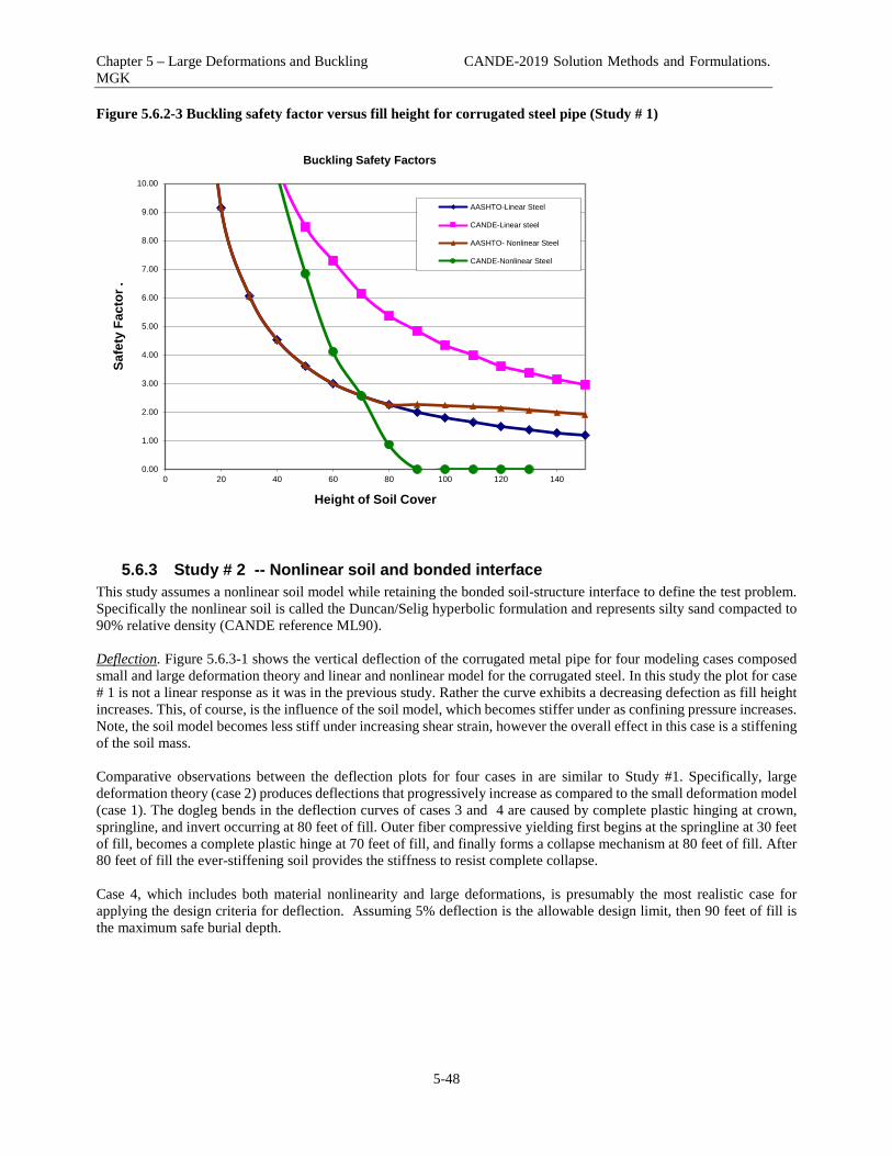
Chapter 5 – Large Deformations and Buckling CANDE-2019 Solution Methods and Formulations. MGK
5-48
Figure 5.6.2-3 Buckling safety factor versus fill height for corrugated steel pipe (Study # 1)
5.6.3 Study # 2 -- Nonlinear soil and bonded interface This study assumes a nonlinear soil model while retaining the bonded soil-structure interface to define the test problem. Specifically the nonlinear soil is called the Duncan/Selig hyperbolic formulation and represents silty sand compacted to 90% relative density (CANDE reference ML90). Deflection. Figure 5.6.3-1 shows the vertical deflection of the corrugated metal pipe for four modeling cases composed small and large deformation theory and linear and nonlinear model for the corrugated steel. In this study the plot for case # 1 is not a linear response as it was in the previous study. Rather the curve exhibits a decreasing defection as fill height increases. This, of course, is the influence of the soil model, which becomes stiffer under as confining pressure increases. Note, the soil model becomes less stiff under increasing shear strain, however the overall effect in this case is a stiffening of the soil mass. Comparative observations between the deflection plots for four cases in are similar to Study #1. Specifically, large deformation theory (case 2) produces deflections that progressively increase as compared to the small deformation model (case 1). The dogleg bends in the deflection curves of cases 3 and 4 are caused by complete plastic hinging at crown, springline, and invert occurring at 80 feet of fill. Outer fiber compressive yielding first begins at the springline at 30 feet of fill, becomes a complete plastic hinge at 70 feet of fill, and finally forms a collapse mechanism at 80 feet of fill. After 80 feet of fill the ever-stiffening soil provides the stiffness to resist complete collapse. Case 4, which includes both material nonlinearity and large deformations, is presumably the most realistic case for applying the design criteria for deflection. Assuming 5% deflection is the allowable design limit, then 90 feet of fill is the maximum safe burial depth.
0.00
1.00
2.00
3.00
4.00
5.00
6.00
7.00
8.00
9.00
10.00
0 20 40 60 80 100 120 140
Safe
ty F
acto
r .
Height of Soil Cover
Buckling Safety Factors
AASHTO-Linear Steel
CANDE-Linear steel
AASHTO- Nonlinear Steel
CANDE-Nonlinear Steel

Chapter 5 – Large Deformations and Buckling CANDE-2019 Solution Methods and Formulations. MGK
5-49
Figure 5.6.3-1 Load-Deflection plots of corrugated metal pipe (Study # 2)
Thrust stress. Figure 5.6.3-2 shows the load-thrust plots for the same four cases. In all cases the maximum thrust stress occurs at the springline. The thrust stress responses in this figure are very similar to Study #1. Overall, the effect of the nonlinear soil model is to reduce thrust stress values by about 5%, otherwise the shape of the curves and behavior is the same. Again we conclude that the thrust response is fairly insensitive to large deformations. As discussed in the previous study, the abrupt change of thrust behavior in cases 3 and 4 is to be expected because the combination of thrusts and moments has produced complete plastic penetration of the corrugated cross-section at the crown, springline and invert so that the pipe now has minimal hoop stiffness (like slotted joints) which forces the soil to carry the bulk of the additional overburden pressure. As mentioned before, cases 3 and 4 do not produce a maximum thrust stress that approaches the yield stress value of 33,000 psi even at 160 feet of fill. This result reinforces the notion that the design criteria for corrugated metal should include a limit on the allowable plastic penetration because thrust stress alone can be misleading.
0
20
40
60
80
100
120
140
160
180
0 2 4 6 8 10 12 14
Hei
ght o
f Cov
er S
oil (
feet
) .
Percent Deflection
Load-Deformation plots
#1 - All Linear
#2 - Large Deform
#3 - Metal plastic
#4 - Large D+Plastic

Chapter 5 – Large Deformations and Buckling CANDE-2019 Solution Methods and Formulations. MGK
5-50
Figure 5.6.3-2 Load-Thrust stress plots of corrugated steel pipe (Study # 2).
Buckling Stress and Safety Factor. The last comparison for Study # 2 is the buckling load and associated safety factor. Table 5.6.3-1 lists CANDE’s prediction for the thrust stress level that will produce a singular system matrix for each load increment. Of course, the CANDE predictions, which are based on large deformation theory, only apply to cases 2 and 4. As explained in Study # 1, the table also contains the simplified AASHTO prediction for ASSHTO buckling stress and the Chelapatti-Allgood prediction. Table 5.6.3-1. Buckling stress predictions for Study # 2
Fill Height
(feet)
Predicted Thrust Stress Level For Buckling-like Response (psi) CANDE – (#2) Linear steel
CANDE – (#4) Nonlinear steel
ASSHTO Prediction
Chelapatti-Allgood
10 107174 107174 42,867 54,257 20 105029 105029 42,867 54,257 30 106067 109260 42,867 54,257 40 111191 102047 42,867 54,257 50 116490 98317 42,867 54,257 60 123310 88218 42,867 54,257 70 131538 67710 42,867 54,257 80 136658 37562 42,867 54,257 90 142060 0 42,867 54,257
100 150731 0 42,867 54,257 160 175659 0 42,867 54,257
0
20
40
60
80
100
120
140
160
180
0 5000 10000 15000 20000 25000 30000 35000 40000
Hei
ght o
f Soi
l Cov
er (f
eet)
.
Maximum Thrust Stress (psi)
Load-Thrust Relationship
#1 - All Linear#2 - Large Deform#3 - Metal plastic#4 - Large D+Plastic
Full plastic penetration at crown, springline and invert for cases 3 and 4.

Chapter 5 – Large Deformations and Buckling CANDE-2019 Solution Methods and Formulations. MGK
5-51
For the case of linear steel, CANDE’s prediction for buckling capacity increases steadily at each load step because the soil stiffness is increasing without a loss in structural stiffness. However for the case of nonlinear steel, the CANDE predictions for buckling stress begin to steadily decrease as the steel begins to yield at about 40 feet of fill. When the complete collapse mechanism has formed at 80+ feet of fill, the buckling capacity approaches zero. Recall that CANDE’s prediction of buckling stress is based on the current system stiffness matrix that becomes less and less robust as steel yielding increases with each load step. The following figure shows the buckling safety factors as a function of fill height. Safety factors are defined as the buckling stress capacity listed in the above table divided by the corresponding thrust stress shown in Figure 5.6.3-2. Note that the loading axis in the figure has been switched to the horizontal in order to illustrate the decrease in safety as fill height increases. Figure 5.6.3-3. Buckling safety factor versus fill height for corrugated steel pipe (Study #2)
In the above figure we can make the same observations as we did in Study # 1. Namely for the case of linear steel, the AASHTO buckling safety factor is more conservative than CANDE prediction for all stages of fill height. However when comparison is made for cases including yielding steel, the AASHTO safety factor predictions become less conservative after 80 feet of fill. That is the AASHTO safety factor stays relatively constant due to the nearly constant thrust stress from the nonlinear steel solution. In contrast to AASHTO, the CANDE safety factor rapidly decreases due to the rapid loss of buckling capacity such that, after 80 feet of fill, CANDE provides a more conservative (and accurate) prediction of buckling safety than does the AASHTO prediction. Again, it is concluded that the AASHTO prediction for global is buckling is not always conservative.
0.00
1.00
2.00
3.00
4.00
5.00
6.00
7.00
8.00
9.00
10.00
0 50 100 150
Safe
ty F
acto
r
Height of Soil Cover (feet)
Buckling Safety Factors
AASHTO-Linear SteelCANDE-Linear steelAASHTO- Nonlinear SteelCANDE-Nonlinear Steel

Chapter 5 – Large Deformations and Buckling CANDE-2019 Solution Methods and Formulations. MGK
5-52
5.6.4 Study # 3 -- Linear soil and frictionless interface Like the first study, Study # 3 uses a linear soil model, however the soil-structure interface is now assumed to be frictionless. The frictionless interface also infers that the culvert will separate from the soil if tension forces should occur. Deflection. Figure 8 shows the vertical deflection of the corrugated metal pipe for three modeling cases: (the case of steel yielding with small deformations is no longer of interest)
(1) linear steel material and small deformation theory (2) linear steel material and large deformation theory (3) yielding steel material and large deformation theory
Figure 5.6.4-1 Load-Deflection plots of corrugated steel pipe (Study # 3)
The load-deflection curves for Study 3 are similar to the corresponding curves in Study 1except that all displacements in the above figure are somewhat larger. In the case of combined large deformations and steel yielding, the deflections become excessive at 100 feet fill. This is because at 90 feet of fill the steel at the crown and the invert begin to buckle inward and separates from the soil due to tension break in the interface model. This causes the large displacement observed at 100 feet of fill in the above figure. Thrust stress. Figure 5.6.4-2 shows the load-thrust plots for the same three cases. In all cases the maximum thrust stress occurs at the springline. Again, the thrust-load plots are similar to the corresponding plots in Study # 1 except that all thrusts are somewhat lower than the completely bonded case. This result is ascribed to loss of shear traction in the frictionless case. For case # 3, the combination of thrust and moment form a collapse mechanism at about 80 feet of fill so that further increase in thrust stress is retarded
0
20
40
60
80
100
120
140
160
180
0 2 4 6 8 10 12 14
Hei
ght o
f Cov
er S
oil (
feet
) .
Percent Deflection
Load-Deformation plots
#1 - All Linear
#2 - Large Deform
#3 - Large D+Plastic

Chapter 5 – Large Deformations and Buckling CANDE-2019 Solution Methods and Formulations. MGK
5-53
Figure 5.6.4-2. Load-Thrust stress plots of corrugated metal pipe (Study # 3).
Buckling Stress and Safety Factor. The last comparison for Study # 3 is the buckling capacity and associated safety factor. Table 5.6.4-1 lists CANDE’s prediction for the thrust stress level that will produce a singular system matrix for each load increment. The table also contains the simplified AASHTO prediction for ASSHTO buckling stress and the Chelapatti-Allgood prediction. Table 5.6.4-1 Buckling stress predictions for Study #3
Fill Height
(feet)
Predicted Thrust Stress Level For Buckling-like Response (psi)
CANDE – (#2) Linear steel
CANDE – (#3) Nonlinear steel
ASSHTO Prediction
Chelapatti-Allgood
10 84219 84219 42,867 54,257 20 84318 84318 42,867 54,257 30 83282 83663 42,867 54,257 40 82244 77324 42,867 54,257 50 83348 64154 42,867 54,257 60 83256 43962 42,867 54,257 70 81915 27274 42,867 54,257 80 81140 4196 42,867 54,257 90 83076 0 42,867 54,257
100 82295 0 42,867 54,257 160 83145 0 42,867 54,257
For the case of linear steel, the predicted buckling stress remains relatively constant at a nominal value of 83,000 psi, which is about 20% less than the corresponding predictions in Study # 1. The 20% reduction is attributed to the observation that the frictionless interface does not generate the same amount of shear stiffness in the soil as does the fully bonded condition. Note that the Chelapati-Algood model is completely devoid of shear stiffness, which is one reason that their buckling predictions are on the low side.
0
20
40
60
80
100
120
140
160
180
0 5000 10000 15000 20000 25000 30000 35000 40000
Hei
ght o
f Soi
l Cov
er (f
eet)
.
Maximum Thrust Stress (psi)
Load-Thrust relationship
#1 - All Linear
#2 - Large Deform
#3 - Large D+Plastic
Full plastic penetration at crown, springline and invert for case 3 at 80 feet.
Steel buckles away from soil at crown and invert for case 3 at 90 feet ( interface seprates).

Chapter 5 – Large Deformations and Buckling CANDE-2019 Solution Methods and Formulations. MGK
5-54
As observed in the previous studies, the CANDE predictions for buckling stress in the presence of yielding steel begin to steadily decrease as the steel begins to yield between 30 and 40 feet of fill. When the complete collapse mechanism has formed at 80+ feet of fill, the buckling capacity approaches zero. Figure 5.6.4-3 shows the buckling safety factors as a function of fill height. Safety factors are defined as the buckling stress capacity listed in the above table divided by the corresponding thrust stress shown in Figure 5.6.4-2. Again it is observed that in the case of yielding steel, the CANDE safety factor rapidly decreases due to the rapid loss of buckling capacity. After 60 feet of fill, CANDE provides a more conservative (and accurate) prediction of buckling safety than does the AASHTO prediction. Figure 5.6.4-3 Buckling safety factor versus fill height for corrugated metal pipe (Study #3)
5.6.5 Comparing Studies #1, #2 and #3 with design criteria We conclude this chapter by comparing the maximum allowable fill heights for the three studies based on working-stress design criteria for corrugated steel pipe. Restricting the comparison to the cases of large deformation with steel yielding, which are presumably the most realistic CANDE solutions, the three studies are differentiated as follows:
• Study #1 = linear soil with bonded interface, • Study #2 = nonlinear soil with bonded interface • Study #3 = linear soil with frictionless interface
The design criteria and safety factors are given in the table below,
0.00
1.00
2.00
3.00
4.00
5.00
6.00
7.00
8.00
9.00
10.00
0 20 40 60 80 100 120 140
Safe
ty F
acto
r .
Height of Soil Cover (feet)
Buckling Safety Factors
AASHTO-Linear Steel
CANDE-Linear steel
CANDE-Nonlinear Steel

Chapter 5 – Large Deformations and Buckling CANDE-2019 Solution Methods and Formulations. MGK
5-55
Table 5.6.5-1 Working stress design criteria for corrugated metal pipe Design Criterion
Safety Factor
Allowable limit
Thrust yielding 2.0 Thrust stress = ½(yield stress) Global buckling 2.0 Thrust stress = ½(buckling prediction)
Plastic penetration 1.5 Amount of wall yielding = 2/3 of depth Vertical deflection 1.0 Deflection = 5% of diameter
Using the above allowable limits and referring to the previous plots for the cases of large deformation with steel yielding, the maximum fill height may be determined for each design criterion. The results for each study are recorded in the table below. Table 5.6.5-2. Allowable fill heights for each design criterion (feet)
Study #
Thrust Yielding
Global Buckling
Plastic Penetration
Vertical Deflection
1 73.0 ft 73.3 ft 55.2 ft 79.5 ft 2 79.4 ft 81.1 ft 49.7 ft 87.7 ft 3 88.9 ft 70.3 ft 53.9 ft 70.9 ft
Plastic penetration is the controlling design criterion for each study, which limits the maximum burial depth on the order of 50 feet. It is interesting to note that all three studies (installation conditions) have both strengths and weaknesses with regard to the design criteria. As a final comment, the CANDE program performed in a robust manner to obtain converged solutions with several nonlinear models being exercised simultaneously

Chapter 6 – Design Criteria and LRFD Design Methodology CANDE-2019 Solution Methods and Formulations. MGK
6-1
DESIGN CRITERIA AND LRFD DESIGN METHODOLGY Inroduction. The probabilistic-based design philosophy known as load and resistance factor design (LRFD) has been adopted into the AASHTO LRFD Bridge Design Specifications (Reference 6) wherein the specifications for buried structures are primarily contained in Section 12. One of the tasks in the NCHRP CANDE Upgrade project was to incorporate LRFD methodology for all culvert materials into CANDE-2019 in addition to the traditional working stress design (WSD) methodology. This chapter provides a succinct interpretation of the AASHTO LRFD specifications for buried structures with regard to defining factored loads and establishing design criteria. Tabularized values are summarized in this chapter for load factors and load modifiers to quantify dead loads, earth loads, and live loads, which are required for a LRFD analysis to produce the factored demands. The contents of this chapter are published in the Transportation Research Record No. 2028, Reference 23. Also presented are tabularized descriptions of the design criteria and the corresponding factored capacities, which are defined and quantified herein for corrugated metal, reinforced concrete, and plastic pipe materials. In some cases, the design criteria have been generalized to provide mechanistically meaningful statements that are compatible with comprehensive analysis methods like CANDE. Although this chapter is focused on LRFD design methodology, the fundamental design criteria presented herein are also used for CANDE’s WSD methodology. The WSD approach uses service loads and unfactored capacities to compute safety factors defined as capacity divided by service-load demand. The LRFD approach uses factored loads and factored capacities to compute ratios of factored demand divided by factored capacity for strength related design criteria, and service-load demand divided by performance limits for service-related design criteria. The objectives of this chapter are as follows:
• Summarize the loading definitions and load factors for LRFD methodology that are applicable to the comprehensive solution approach embodied in the CANDE-2019 program.
• Provide a clear and concise set of design criteria for buried structures for corrugated metal, reinforced concrete
and plastic pipe that are mechanistically consistent with AASHTO LRFD specifications, but are not dependent on simplified design equations.
• Identify areas where improvements in the current AASHTO specifications are desirable and offer suggestions
for a more generalized statement of the design criteria. LRFD methodology for buried structures includes both service limit states and strength limit states. One consequence of the two limit states when using a comprehensive solution method is that two separate solutions may need to be obtained, one with service loading and one with factored loading. The definitions of service loading and factored loading are provided in the following discussion along with tables summarizing the specified load factors. To augment this discussion, guidance is provided on applying these factored loads in the context of a comprehensive finite element solution methodology.

Chapter 6 – Design Criteria and LRFD Design Methodology CANDE-2019 Solution Methods and Formulations. MGK
6-2
6.1 Service Loads for Performance Criteria A common example of performance criteria under service loading is the allowable deflection of flexible culverts. In the case of rigid culverts, a common example is the allowable concrete crack width. Later, the exact form of these and other design criteria will be discussed and quantified. For present purposes it is only necessary to understand that a solution at the service load level is required in order to evaluate the service limit design criteria. For a culvert system to successfully pass the service load design criteria, the predicted response such as the percent deflection must be less than or equal to the allowable limit. The service load level is the actual design load experienced by the culvert system as if one were performing a working stress analysis. Service loads include the following conditions:
1. Dead load of structure 2. Earth load on the soil 3. Live load pressure on the structure transmitted through soil 4. Live load multiplier due to vehicle impact 5. Live load multiplier due to multiple lane presence 6. Other design load considerations such as hydrostatic or thermal loading
In terms of finite element modeling, the structure dead load (body weight of the culvert) is typically applied in the first load step after consideration of in situ soils, followed by a sequence of load steps composed of soil element layers, which are placed around and above the culvert up to the design cover height. Each soil layer is loaded with its own body weight according to the soil density associated with the region. Live loads are typically applied in the last load step(s) on the soil surface as a pressure boundary condition, representing the tire footprint pressures from the design-truck. AASHTO specifications also require that service-load tire pressures be increased by multipliers to account for dynamic impact and the effects of multiple lane presence, which are prescribed as follows:
• Impact multiplier = 1 + 0.33( 1.0 – H/8.0) ≥ 1.0 Equation 6-1 where, H is height of soil cover above the crown in feet.
• Multiple-lane-presence multiplier = 1.2 Equation 6-2 The multiple lane presence factor is 1.2 for a single loaded lane and considers that a single truck has a high likelihood of being overloaded. While LRFD allows reduced values of the multiple presence factor when more than one lane is loaded, calculations for culverts under live load show that the single loaded lane condition virtually always controls the design. As a side comment, it is noted that the prescription of the basic live load tire pressure presents a special problem for two-dimensional, plane strain finite element programs because the tire foot print area extends to infinity in the out-of-plane direction, thereby overestimating the actual loading on the culvert as compared to the actual footprint width of finite dimensions. One way to correct for this problem is to reduce the surface pressure using the procedure described in Reference 12 and Reference 13. Other methods are currently being invested under NCHRP Project 15-29.

Chapter 6 – Design Criteria and LRFD Design Methodology CANDE-2019 Solution Methods and Formulations. MGK
6-3
6.2 LRFD Loads for Strength-limit States For strength limit states such as the yield strength, ultimate strain, or global buckling capacity of the soil-structure system, the LRFD methodology assigns net multiplying factors to the service loads. The resulting structural responses, which are at higher levels of stress than the service load responses, are called the factored demands. Concurrently, resistance factors, whose values are typically 1.0 or less, are multiplied by the strength values and the resulting products are called factored capacities. The test of a successful culvert design using the LRFD methodology is that the factored capacities are greater or equal to the corresponding factored demands for all the strength-state design criteria. In a simplistic sense, the ratio of the effective load factor to the resistance factor is comparable to the safety factor concept used in working stress design methodology. However, it is generally accepted that LRFD methodology offers a more logical design assessment than WSD methodology. The net multiplying factor applied to service loads is product of two terms called the load factor and the net load modifier. Stated explicitly, the net factored load at any load step may be written as: Factored load = γ η (Service load) Equation 6-3 where, γ is the specified load factor, and η is the net load multiplier.
6.2.1 Load Factors. The load factor term, symbolically denoted as γ, is currently specified in AASHTO LRFD specifications as shown in the table below. A general observation that should fit well with reader’s intuition is that γmax (on average) increases in value from the dead load case to the earth load case to the live load case. This increase in load factor value roughly corresponds with our lack-of-confidence in knowing the actual load value in these three cases. TABLE 6.4.1-1 Load factors and load modifiers for buried structures
Culvert Type Dead Load Culvert (DC)
Earth fill Loading (EB)
Live Load (LL)
γmax γmin ηDC γmax γmin ηEB γmax ηLL Reinforced Concrete pipe
1.25 0.9 1.05 1.3 0.9 1.05 1.75 1.00
Reinforced Concrete box
1.25 0.9 1.05 1.3 0.9 1.05 1.75 1.00
Reinforced Concrete arch
1.25 0.9 1.05 1.3 0.9 1.05 1.75 1.00
Corrugated metal pipe or arch
1.25 0.9 1.05 1.95 0.9 1.05 1.75 1.00
Corrugated metal box
1.25 0.9 1.05 1.50 0.9 1.05 1.75 1.00
Plastic pipe (HDPE or PVC)
1.25 0.9 1.05 1.95 0.9 1.05 1.75 1.00
Symbols: γmax = maximum load factor dependent on load case and culvert type. γmin = minimum load factor dependent on load case and culvert type. ηDC = net load modifier for DC load case = {(ductility)(redundancy)(importance)} ηEB = net load modifier for EB load case = {(ductility)(redundancy)(importance)} ηLL = net load modifier for LL load case = {(ductility)(redundancy)(importance)} Two observations about the load factors in Table 1 that require further explanation are; (1) there are two values, γmax and γmin, listed for each load case, and (2) the load factors are dependent on the type of culvert material and shape. With regard to the first observation, the maximum load factor, γmax, is generally the value used in an analysis to produce the worst-case structural response. However during the sequence of load steps in a comprehensive solution method, it is conceivable that for some load steps the consistent application of γmax may not produce a worst case scenario for a given

Chapter 6 – Design Criteria and LRFD Design Methodology CANDE-2019 Solution Methods and Formulations. MGK
6-4
design criteria. For example, if the earth-fill layers of soil are heavily compacted along the sides of the culvert so that lateral pressure causes an inward movement, the resulting change in moments in the culvert may become less than the initial moment caused by the dead load of culvert in step 1, and also counter to the sign of the moments that will be added into the culvert when subsequent earth-fill layers are placed on top of the culvert. Thus in the spirit of seeking the worst-case LFRD loading scenario, it may be reasonable to use γmin for those load steps wherein earth-load layers are placed along the sides of the culvert. The second observation, i.e., the load factor values are dependent on culvert type and shape, does not have a rational explanation except to say the AASHTO specifications represent work-in-progress. It is certainly reasonable to assign different resistance factors to different structural materials; however it is difficult to argue why the load factors, such as those for vertical earth load, should be different. Perhaps at some time in the future, the load factors will be uniform for all buried structures. However until that time comes, Table 1 serves as the reference for load factors.
6.2.2 Load Modifiers. The so-called net load modifier, symbolically denoted as η , is a product of three sub-factors related to ductility, redundancy and operational importance that are described in AASHTO LRFD Specifications 1.3.2.1. For buried structures it is customary to assign the sub-factors associated with ductility and operational importance to be 1.0. However for the redundancy sub-factor the LRFD specification suggests that value should be 1.05 for buried structures under dead loads and earth loads, but not live loads. Based on the above discussion, the values in Table 6.4.1-1 for ηDC and ηEB are recommended to be 1.05 when the maximum load factor γmax is being used. On the other hand, if the minimum load factor γmin is assigned to a particular load step, then the corresponding load modifier is the inverse value, e.g. load modifier = 1/1.05 = 0.95. The load modifier for operational importance is a function of the specific structure being designed, thus, while often set to 1.0, other values may be appropriate. The above loading conditions are not a recipe for all culvert problems because worst loading scenario depends on the structure type, installation, and the governing limit state. However, the beauty of comprehensive solution procedures like CANDE is that it easy to re-run the same problem with different load factors to find the worst loading condition.
6.2.3 LRFD load factors and nonlinear soil models. A long-standing issue with regard to LRFD analysis is whether or not nonlinear soil models should be driven by stresses and strains from factored loading or from service loading. Although there is no question that factored loads are required to produce the factored demands to evaluate the LRFD design criteria against the factored capacities, some engineers argue that the factored soil stresses and strains cause the nonlinear soil models to become overly stiff due to the increased confining pressure from factored loads, especially for the case of deep burial wherein nonlinear soil models like the Duncan/Selig hyperbolic soil models generally result in substantially increased soil stiffness due to “artificially” increased confining stress from the earth load factor. Others argue that the LRFD philosophy implies that factored loads have some “real” probability of occurring so that the increased soil stiffness is the proper analysis approach. Of course, this dilemma only applies to nonlinear soil models because linear soil models are insensitive to the level of stress. Rather than adopting only one method or the other in the CANDE-2019 program, the Duncan/Selig soil model is programmed to operate by either method at the user’s option. Specifically, the input variable called NON in the Duncan/Selig input instructions allows the user to choose whether "service stresses" (NON = 0) or "factored stresses" (NON =1) are used to compute the Duncan/Selig stiffness values for Young's modulus and Bulk modulus. Thus even though factored loads are input into CANDE and the solution output are actual factored structural responses, for the case NON = 0, the stiffness calculations performed within the Duncan/Selig subroutine are based on service stresses at each load step. This is achieved by dividing the factored stress and strain increments by the corresponding load factor for that load step and maintaining a running total of the service stresses and strains to drive the nonlinear soil model.

Chapter 6 – Design Criteria and LRFD Design Methodology CANDE-2019 Solution Methods and Formulations. MGK
6-5
6.3 Design Criteria for Culvert Materials In the following paragraphs, the AASHTO LRFD design criteria are regrouped into three material types called corrugated metal, reinforced concrete, and plastic pipe. The design criteria are summarized in tables followed by a discussion of each design criterion. The tables list the resistance factors, factored capacities and the corresponding reference to AASHTO LRFD Specification. We believe the tabularized design criteria accurately reflect the intentions of the AASHTO specifications; however in some cases, denoted with an asterisk, we have generalized the criterion to be mechanistically compatible with comprehensive solution methods like CANDE-2019.
6.3.1 Corrugated metal Corrugated steel and corrugated aluminum have the same general AASHTO design criteria, differing only by the numerical value of design criterion limits such as the yield stress. Table 2 is applicable to both types of corrugated metal. The criterion for plastic penetration is a generalization of the AASHTO specifications and is discussed below. Table 6.5.1-1 Corrugated Metal LRFD Design Criteria.
Design Criterion (Strength limits)
Resistance Factor
Factored Capacity
Definition and AASHTO Reference
(1) Thrust stress (psi) φ1 = 1.0 φ1F1 F1 = metal yield strength (Equation 12.7.2.3-1.)
(2) Global Buckling (psi) φ2 = 1.0 φ2F2 F2 = buckling thrust stress (Equations 12.7.2.4-1-2)
(3) Seam strength (psi) φ3 = 0.67, 1.0 φ3F3 F3 = seam strength (Section 12.7.2.5)
(4) Plastic Penetration *(%) φ4 = 0.90 φ4F4 F4 = fully plastic (100%) (Replaces 12.9.4.3.1)
Performance Limits ( Service Load)
(5) Allowable deflection *(%) -- P5 P5 = 5%, (2% LS)
1. The thrust stress limit value, F1, is typically 33,000 psi for steel and 24,000 psi for aluminum. The thrust stress criterion is based on AASHTO LRFD equation 12.7.2.3-1.
2. The thrust stress level that causes global buckling, F2, may be conservatively approximated from the simplified
AASHTO LRFD equations 12.7.2.4-1-2. A more accurate alternative is to utilize the new large deformation formulation with buckling capacity prediction available in CANDE-2019
3. If seams are not present, the factored seam strength value φ3F3 may be set equal to F1. If longitudinal seams
are present, F3 should represent the measured seam capacity and φ3 = 0.67 4. Failure from full plastic penetration occurs when the cross section becomes fully plastic due to plastic hinging,
which occurs when the internal moment approaches the plastic moment capacity (F4 = 100%). The recommended LRFD resistance factors are 0.90 for steel and 0.85 for aluminum, respectively. This criterion is a generalization of the original AASHTO LRFD equation 12.9.4.3.1 for structural plate box culverts.
AASHTO specifications are silent on limiting moments or plastic hinging for corrugated metal structures other than structural plate box structures. As implied in the above table, we believe plastic penetration design criterion should applicable to all corrugated metal structures including pipes, arches and long spans.
5. The service load limit for allowable deflection, P5, is generally taken as 5% for all corrugated metal structures
except long spans, which are usually limited to 2% of the vertical rise. Although AASHTO Bridge Specification does not currently specify deflection limits, experience has shown that deflections greater than 5% indicate that the backfill type and/or compaction are below standard.

Chapter 6 – Design Criteria and LRFD Design Methodology CANDE-2019 Solution Methods and Formulations. MGK
6-6
6.3.2 Reinforced concrete The AASHTO design criteria for reinforced concrete are the most challenging criteria to generalize because the criteria are masked in simplified solution methods and are differentiated for various culvert shapes. In Table 6.5.2-1 and the ensuing discussion, it is believed that the proposed design criteria faithfully represent the intent and in some cases improve the clarity of the criteria as presented in the AASHTO LRFD specifications. Table 6.5.2-1 Reinforced Concrete LRFD Design Criteria
Design Criterion (Strength limits)
Resistance Factor
Factored Capacity
Definition and AASHTO Reference
(1) Steel yielding (psi) φ1 = 0.90 φ1F1 F1 = reinforcement strength (Alternative to 12.10.4.2.4a-1)
(2) Concrete crushing* (psi) φ2 = 0.75 φ2F2 F2 = concrete strength (New proposed criterion)
(3) Shear failure (lb/in) φ3 = 0.90 φ3F3 F3 = concrete shear strength (Multiple AASHTO equations)
(4) Radial tension failure (psi) φ4 = 0.90 φ4F4 F4 = radial tension strength (Adapted from 12.10.4.2.4c-1)
Performance Limits ( Service Load)
(5) Allowable crack width* (in) -- P5 P5 = 0.01 inch (Recommendation)
1. The steel yielding stress limit value, F1, is nominally 60,000 psi for deformed bars and 65,000 psi for smooth
wire fabric. This criterion is a generalization of AASHTO LRFD Equation 12.10.4.2.4a-1 and more fundamental then the AASHTO equation for steel area. Note that the AASHTO equation specifies the required steel area for the steel-yielding criterion based on a simplified solution method.
2. The outer-fiber concrete crushing stress limit value, F2, is the ultimate compressive strength fc’. A concrete
compression criterion is explicitly stated in the AASHTO LRFD specifications because it is assumed that reinforcing steel is designed to yield prior to the load level causing the concrete to begin crushing. Here it is proposed that concrete crushing should be retained as a direct design criterion and the specified resistance factor for concrete crushing be less than specified the resistance factor for steel yielding, with values of 0.75 and 0.90, respectively.
3. The shear capacity, F3, is the shear force causing diagonal tension failure at a given cross-section. If the shear
demand exceeds the shear capacity, then transverse reinforcement (stirrups) is required. The value of F3 is specified differently by AASHTO depending on structural shape and burial depth.
• For concrete pipes and arches, the shear strength is specified by Equations 12.10.4.2.5, which yield
a variable value for F3 dependent on the values for moment, thrust and shear around the culvert wall.
• For boxes and 3-sided structures with 2 or more feet of soil cover, the shear strength is specified
by Equations 5.14.5.3-1 wherein the value for F3 is dependent on moment and shear (not thrust).
• For boxes and 3-sided structures with less than 2 feet of soil cover, the shear strength is specified by equations in Section 5.8.3.3 that, in some cases, depend on the nature of the traverse reinforcement (stirrups).
Clearly there is a need for unifying the AASHTO LRFD specifications for the shear strength capacity because rational mechanics suggests that shear strength capacity should be a function of the cross-section properties and state of loading, not on the culvert shape or depth of burial. Hopefully this remark may stimulate a future research study to develop a more fundamental criterion, which is the root cause of diagonal cracking. However until that

Chapter 6 – Design Criteria and LRFD Design Methodology CANDE-2019 Solution Methods and Formulations. MGK
6-7
time, we propose that AASHTO Equation 12.10.4.2.5 is the best predictor of shear strength capacity for culverts because of the large experimental data base upon which it was developed (Reference 14).
4. The radial tension failure stress, F4, is related to the tension strength of concrete and the structure span. The
criterion is adapted from AASHTO LRFD equation 12.10.4.2.4c-1. It is restated here in psi units as:
F4 = 37.92(fc’/1000)1/2 Frt Equation 6-4
where Frt is a scale factor dependent on structure span, which is specified in the paragraphs following Equation 12.10.4.2.4c-1.
The corresponding factored demand is the average radial tensile stress that the curved inner cage exerts on the inside concrete cover thickness. This is automatically determined in CANDE-2019 by dividing the interior cage steel force (maximum tensile force per unit length) by the radius of curvature of the steel cage.
5. The allowable crack width at service loading is generally taken as 0.01 inches in accordance with AASHTO
LRFD specification 12.10.3. An empirical formula to predict crack width, developed by Heger and McGrath (Reference 15), has been adopted by AASHTO in the form of Equation 12.10.4.2.4d-1. For purposes of this paper, the authors reworked the equation in a more fundamental form, which linearly relates crack width to the tension stress in the reinforcing steel once it exceeds the surrounding concrete tensile strength. The revised equation is:
CW = (tbsl / 2n)1/3{fs – 0.0316C1(h/d)2√fc’/ρ}/3000 Equation 6-5
where, CW is crack width in inches, ≥ 0 fs is tension steel stress in ksi units fc’ is concrete strength in ksi units All other symbols are section properties defined in Section 12.10.4.2.4d
CANDE-2019 predicts the crack width at each point around the culvert by feeding the computed tension steel stress fs into Equation 5.6 thereby producing a semi-empirical prediction. This procedure has been well calibrated for crack widths of approximately 0.01 in. and becomes increasingly uncertain as the crack width varies from this value. As an alternative, CANDE provides the option to use the older Gergely-Lutz formula instead of Equation 6-5.
6.3.3 Plastic pipe The design criteria for plastic pipe, summarized in Table 6.5.3-1, are straightforward interpretations of the AASHTO LRFD specifications. Said another way, the AASHTO fundamental design criteria are easily understood and not confounded with the simplified methods that are offered to predict the factored demands. The main difficulty in applying the plastic pipe design criteria is deciding whether to use the long-term or short-term material properties. Typically, an engineer would select short-term material properties if live loads were the major concern. On the other hand, for deep burial situations long-term properties are appropriate. In some cases, it may be prudent to solve the problem twice, once with short-term properties and once with long-term properties. This is a relatively easy task with CANDE-2019.

Chapter 6 – Design Criteria and LRFD Design Methodology CANDE-2019 Solution Methods and Formulations. MGK
6-8
Table 6.5.3-1 Plastic Pipe LRFD Design Criteria. Design Criterion (Strength limits)
Resistance Factor
Factored Capacity
Definitions and AASHTO Reference
(1) Thrust failure (psi) φ1 = 1.0 φ1F1 F1 = plastic yield strength (Equation 12.12.3.5.1)
(2) Global buckling (psi) φ2 = 1.0 φ2F2 F2 = thrust stress for buckling (Equation 12.12.3.5.2-1)
(3) Combined strain (in/in) φ3 = 1.0 φ3F3 F3 = fiber strain limit (Equation 12.12.3.5.4a-1)
Performance Limits ( Service Load)
(4) Allowable displacement (%)
-- P4 P4 = 5% (Recommendation)
(5) Allowable tensile strain (in/in)
-- P5 P5 = 0.05 (for HDPE) (Table 12.12.3.3-1)
1. The thrust stress limit or ultimate strength, F1, is dependent on the type plastic and the load duration. Types of
plastic identified by AASHTO include high-density polyethylene (HDPE) and polyvinyl chloride (PVC) with characteristic material properties for short-term or long-term loading. Nominal values, taken from the ASSHTO LRFD specifications and elsewhere, are shown in Table 6.5.3-2. Thrust load capacity is also influenced by profile geometry, which can reduce section capacity due to susceptibility to local buckling as discussed below.
Table 6.6.3-2 Recommended plastic properties for short and long-term loading
Type of plastic
Effective Young’s Modulus (PE)
Ultimate strength (PU)
Short-term (ksi)
Long-term (ksi)
Short-term (ksi)
Long-term (ksi)
HDPE –
110.0
22.0
3.00
0.90
PVC –
400.0
140.0
6.00
2.60
PP –
135.0
27.0
3.10
1.00
2. The thrust stress level that causes local global buckling, F2, may be conservatively approximated from the simplified AASHTO LRFD equations 12.7.2.4-1-2. A more accurate alternative is to utilize the new large deformation formulation with buckling capacity prediction available in CANDE-2019.
3. The combined strain limit value (combined thrust and bending), F3, is specified by AASHTO LRFD Equation
12.12.3.5.4a-1 and is equal to 1.5 times the long-term strength divided by the long-term modulus. Accordingly, HDPE ~ 0.06 in/in, PVC ~ 0.028 in/in. and PP ~ 0.045 in/in.
4. The service load value for allowable deflection, P4, is generally taken as 5% of the diameter for all plastic pipes;
however, the deflection limit is not directly specified in the AASHTO LRFD Design Specifications. 5. The service load value for maximum allowable tensile strain, P5, is specified in AASHTO LRFD table
12.12.3.3-1 and is 0.05 in/in for HDPE and 0.035 or 0.05 in/in for PVC depending on cell class. Local Buckling. Local buckling is not a direct design criterion for plastic pipe, but it does influence the demands and capacities of the design criteria listed above. Local buckling is a nonlinear phenomenon caused by compressive forces that induce the sub elements of profile wall pipe to deform out-of-plane in a wrinkled pattern. Similar to corrugated metal

Chapter 6 – Design Criteria and LRFD Design Methodology CANDE-2019 Solution Methods and Formulations. MGK
6-9
pipe wherein some amount of outer fiber yielding is permitted, some amount of local buckling is permitted in plastic profile pipe. Chapter 2 provides a description of the CANDE’s nonlinear model to account for local buckling based on Section 12.12.3.5.3 of AASHTO LRFD specifications. The procedure simulates the effect of local buckling by reducing the effective area of the sub elements dependent upon the average level of compressive strain in each sub element. Thus, local buckling increases the demand and/or decreases the capacity of design criteria listed above.
6.4 Illustration of LRFD Factors and Evaluation with CANDE This example is for a concrete arch with straight legs installed in a trench-like installation with backfill soil placed in eight layers to a final cover height of 2 feet above the crown. A live load is placed over the arch centerline on the ninth and last load increment. To evaluate this problem under LRFD design methodology, CANDE’s Level-2 arch mesh option is used to automatically construct a symmetric finite element mesh with nine construction increments with the load factors taken from Table 6.4.1-1 and computed as described in the following paragraphs.
6.4.1 Construction increment number 1. As shown in Figure 6.6.1-1, the first construction increment includes the surrounding in situ soil (red), concrete footing (yellow), and reinforced concrete arch culvert (black). The in-situ soil and the footing are assigned appropriate stiffness values, but with zero body weight. That is, since the in-situ soil and footing are in place before the arch is constructed, the arch is only loaded with its own self-weight. Thus, the arch is assigned a body weight of 150 pcf, representing body weight of concrete. LRFD analysis requires the user to define the load factor for each construction increment. In this case, the first load step represents dead load (γ = 1.25 and η = 1.05) so that the net load factor = 1.25*1.05 = 1.31.
6.4.2 Construction increment numbers 2 through 8 Figure 6.6.2-1 shows construction increments 2 through 8, which are all associated with earth loading. The 2nd increment is shown as two rows of orange elements, the 3rd increment is shown in yellow, the 4th in green and so on up to the final cover height. Each of these layers of soil is assigned the actual body weight (120 pcf) of the fill soil. Also each increment is assigned the same load factor based on earth loading, computed as (γ = 1.30 and η = 1.05) = 1.37. CANDE applies the load factor to the earth loads in steps 2 through 8 so that the accumulated solution is the factored demand at the end of each step. Figure 6.6.1-1 Concrete arch installation for first construction increment (net load factor =1.31)

Chapter 6 – Design Criteria and LRFD Design Methodology CANDE-2019 Solution Methods and Formulations. MGK
6-10
Figure 6.6.2-1 Concrete arch installation for construction increments 2-8 (net load factor =1.31)
6.4.3 Construction increment number 9 (live load). The last construction increment represents a live load as illustrated by the red circle in the figure below. The load is applied in the 9th step without additional soil loading as a downward force (boundary condition) representing the actual service load of a design truck, but reduced for plane-strain considerations. In this case the net load factor is computed as (γ = 1.75 and η = 1.05) = 1.84. CANDE applies this load factor to the service load as prescribed in the boundary condition. Thus CANDE’s final accumulated solution at the end of load step 9 is the total factored demand. Figure 6.6.3-1 Concrete arch installation for ninth construction increment (net load factor =1.84)

Chapter 6 – Design Criteria and LRFD Design Methodology CANDE-2019 Solution Methods and Formulations. MGK
6-11
6.3.4 Final evaluation of LRFD design criteria The final evaluation of the reinforced concrete arch is shown Figure 6.6.4-1in terms of the design criteria for reinforced concrete. CANDE prints out this evaluation at each load step but our interest is focused on the last load step because it represents the worst case. Here we observe that the concrete arch is safe for the proscribed loading conditions because all demand-to-capacity ratios are less than 1.0. In this example, the steel yielding design criterion is called the controlling design criterion because it has the highest ratio. The controlling node number in the evaluation summary identifies the location in the concrete arch where each design criterion has the maximum demand-to-capacity ratio. Although not shown here, the evaluation summary also includes a performance assessment including the predicted crack width under service load conditions. Figure 6.6.4-1 LRFD evaluation summary for concrete arch after load step 9 (copy from CANDE) LRFD SUMMARY EVALUATION FOR GROUP 1, LOAD STEP 9 DESIGN-CRITERION CONTROL FACTORED FACTORED RATIO NODE DEMAND CAPACITY VALUE STEEL YIELDING (psi) 1 46450.1 54000.0 0.860 CONCRETE CRUSHING (psi) 12 1934.2 3000.0 0.645 SHEAR FAILURE (lbs/in) 11 460.5 782.7 0.588 RADIAL-TENSION FAIL (psi) 1 7.8 54.6 0.142 (Print out from CANDE)

Chapter 7 – Bandwidth Minimization CANDE-2019 Solution Methods and Formulations. MGK
7-1
BANDWIDTH MINIMIZATION
A bandwidth minimizer is installed in CANDE-2019 that reduces the maximum bandwidth of the system of equations characterizing the finite element mesh topology. Bandwidth minimization is achieved by strategically renumbering the node numbers that were originally input by the user. Node renumbering is accomplished heuristically by swapping node numbers, a pair at a time, starting with the node number with the highest bandwidth and exchanging it with another node number that optimally reduces the maximum bandwidth at the first location while not generating a bandwidth at the second location that is greater or equal to the original maximum bandwidth.
7.1 Background and Objectives Background. For any given finite element problem solved by CANDE, the number rows in global stiffness matrix is dictated by the number of nodal unknowns, which defines the number of equations. In contrast, the number of rows in the global stiffness matrix is dependent on the maximum bandwidth, which depends on the nodal numbering pattern, not the number of equations. By judiciously numbering the nodal pattern, the maximum bandwidth can be reduced. The motivations for reducing the maximum bandwidth are, (1) to reduce storage space for the global stiffness matrix whose size is equal to the number of equations times the maximum bandwidth, and (2) to reduce the time required to solve the system of equations, which is proportional to the number of equations times the square of the bandwidth. For Level 2 operations, which use “canned” finite element meshes, a bandwidth minimizer is not necessary because the nodal numbering pattern has been optimized once and for all time. On the other hand for Level 3 operations, which implies a user-defined mesh topology, a bandwidth minimizer can be useful. Although experienced users usually construct nodal numbering patterns that are reasonably close to an optimum pattern, there are situations in which the nodal numbering pattern may differ substantially from optimum. For example, when a pre-existing finite element mesh is altered to include more elements and nodes in a local area, the added nodes are likely to have node numbers that are numerically much larger than the existing nodes in this neighborhood, thereby resulting in an excessively large bandwidth. The bandwidth minimization problem may be formally stated as follows. Given a sparse, n x n, matrix A with components aij, find a permutation of rows and columns (node renumbering pattern) such that all the non-zero components of matrix A reside in a band that is close as possible to the main diagonal. Or expressed mathematically, Minimize{ i-j for i, j = 1 to n: aij ≠ 0}. Beginning in the 1950s, the bandwidth minimization problem received a lot of attention from mathematicians due to the emergence of the computer for solving large systems of equations representing a wide range of applications. The classical Cuthill-McKee algorithm, published in 1969, employs the breadth-first search method to construct a level structure in the context of graph theory. A similar but more efficient algorithm, known as Gibbs-Poole-Stockmeyer, was published in 1976, and remains very popular. Although the above and many other general-purpose bandwidth minimization algorithms are available in the literature, the following development is unique and takes advantage of the finite element assembly methodology to systematically reduce the bandwidth. To the best of the author’s knowledge the bandwidth minimization algorithm presented herein is novel. Objectives. Within the context of the CANDE finite element program and mesh topology, the objectives are;
1. Develop a robust algorithm to convert an arbitrary node-numbering input pattern into a new node-numbering pattern that minimizes the maximum bandwidth. 2. Display all printed and graphical output from the CANDE solutions in terms of the original node-numbering pattern so that the user does not need to learn the new node number scheme, i.e., transparent to user.

Chapter 7 – Bandwidth Minimization CANDE-2019 Solution Methods and Formulations. MGK
7-2
Like other finite element programs, CANDE’s finite element methodology has three properties that are extremely useful for the bandwidth minimization algorithm:
• First, the global system matrix is symmetric so that bandwidth minimization is restricted to one side of the matrix diagonal.
• Second, each node number represents a group of nodal unknowns (e.g., x-displacement, y-displacement, and rotation) each with the same bandwidth. Thus bandwidth minimization is reduced to reordering the node-number pattern as opposed to the entire set of equations.
• Third, all the information required to minimize the bandwidth is contained in the so-called element connectivity matrix, which simply identifies the node numbers associated with each element.
The above advantages are exploited in the following development.
7.2 Bandwidth Minimization Methodology in CANDE
7.2.1 Element connectivity matrix The element connectivity matrix contains the node numbers that are attached to each element and is symbolically denoted and dimensioned as NOD(NET,NDX), where NET is the total number of elements and NDX is the maximum number of nodal locations as required by the various element types. In the CANDE program, for example, NDX = 4 to accommodate the 4-noded quadrilateral elements, which has more nodes than the other types of elements as shown in the table below.
Element Type (connected nodes)
NOD(NE,1) NOD(NE,2) NOD(NE,3) NOD(NE,4)
Beam-column (nodes=2)
Node-1 Node-2 0 0
Triangle (nodes=3)
Node-1 Node-2 Node-3 0
Interface (nodes=3)
Node-1 Node-2 Node-3 0
Quadrilateral (nodes=4)
Node-1 Node-2 Node-3 Node-4
Letting NE be a counter from 1 to NET, then the components of element connectivity matrix are identified as:
• NOD(NE,1) = node number assigned to location 1 of element NE • NOD(NE,2) = node number assigned to location 2 of element NE • NOD(NE,3) = node number assigned to location 3 of element NE (depending on element type) • NOD(NE,4) = node number assigned to location 4 of element NE (depending on element type)
If, for example, element number 10 is a beam element with the two end-nodes numbered 33 and 43, then NOD(10,1) = 33 and NOD(10,2) = 43. The remainder of the nodal list for element 10 is equal to 0.
7.2.2 Algorithm Cycle. With the above information as a starting point, bandwidth minimization is accomplished by swapping node numbers, a pair at a time, starting with a node number that has the highest bandwidth and exchanging it with another node number that optimally reduces the maximum bandwidth at the first node location while not generating a bandwidth at the second location that is greater or equal to the original maximum bandwidth. The process is presented in the following four steps. These steps are repeated iteratively until no additional node pairs can be found to further reduce the bandwidth.

Chapter 7 – Bandwidth Minimization CANDE-2019 Solution Methods and Formulations. MGK
7-3
Step 1. Use the current NOD connectivity matrix to create a new matrix denoted and dimensioned as MT(NDT,3) where NDT is the total number of nodes in the mesh. Letting N represent each node number in turn, the three components of the MT matrix are defined as follows:
• MT(N,1) = Maximum node number among all nodes that are attached to any element that is also attached to node N. MT(N,1) is referred to as NDMAX.
• MT(N,2) = Minimum node number among all nodes that are attached to any element that is also attached to
node N. MT(N,2) is referred to as NDMIN.
• MT(N,3) = Maximum of {ILEFT or IRITE}, where ILEFT = N - NDMIN, which is the bandwidth to the left of node N, and IRITE = NDMAX – N, which is the bandwidth to the right of node N. MT(N,3) is referred to as MAXB, which is the largest bandwidth associated with node N.
The computational key to establishing the MT matrix is to start with an outer do-loop for each node number (referred to as the pivot node). Insert an imbedded do-loop for the element numbering and use the NOD connectivity array. If any of the element’s connectivity nodes match the pivot node, then record the maximum and minimum nodal values found in that element’s connectivity array. Replace the maximum and/or minimum nodal values by node numbers from subsequent element connectivity arrays if the node values are more extreme than the previously recorded values. At completion of the element loop, the values of NDMAX, NDMIN and MAXB for the current pivot node are stored in the MT matrix. Step 2. Search the MT(N,3) column to find the maximum bandwidth of all nodes. Denote and save this value as MAXALL, (i.e., MAXALL = Maximum of {MT(N,3), N=1 to total number of nodes}. It is often the case that several nodes share the same maximum bandwidth value, MAXALL. Accordingly, each of these node numbers is a candidate for the current nodal position to be called node-1. The primary goal is to optimally reduce the bandwidth at the node-1 position by interchanging the node-1 number with an as yet undetermined node number, called node-2. Of course, the insertion of the node-1 number into the node-2 position must also be considered as explained in the next step. Step 3. The purpose of step 3 is to select an optimum pair of nodes, called node-1 and node-2, such that the interchange of their node numbers reduces the local bandwidth at node-1, while maintaining the bandwidth at node-2 to be less than MAXALL. A candidate number for node-1 is labeled N1 and a candidate number for node-2 is labeled N2. We begin with an outer do-loop for all nodes using the node counter N1, and we exclude all N1 node numbers such that MT(3,N1) ≠ MAXALL. Thus, the N1 nodes that are not excluded are candidates for node-1. For node-2 candidates, we use an inner do-loop wherein we restrict our search for N2 node numbers in the sequential range;
N2(start) = MT(1,N1) – MAXALL + 1 N2(end) = MT(2,N1) + MAXALL – 1
This restricted range of N2 contains the only node numbers that will reduce the bandwidth at the N1 position. If the candidate node pair, N1 and N2, were interchanged such that number N2 is assigned to position 1 and number N1 is assigned is assigned to position 2, then the new bandwidths at these two positions can be respectively determined as; MAXB1 = Maximum of {N2-MT(N1,2) or MT(N1,1)-N2} MAXB2 = Maximum of {N1-MT(N2,2) or MT(N2,1)-N1} The next step within the inner loop is to test whether or not the current candidate pair, N1 and N2, is a better choice than the best of the previous candidate pairs. This test is passed by satisfying two simultaneous requirements:
(1) MAXB1 is smaller than that produced by any previous candidate pairs, and (2) MAXB2 is less than MAXALL

Chapter 7 – Bandwidth Minimization CANDE-2019 Solution Methods and Formulations. MGK
7-4
When all candidate node pairs have been tested, there are two possible outcomes, which dictate one of two possible courses of action:
(1) A final node pair, node-1 and node-2, has been identified that reduces the bandwidth. In this case we proceed to Step 4 to update matrices and vectors to perform the node swapping.
(2) No node pair could be found to reduce the current maximum bandwidth (MAXALL). In this case, we exit from
the bandwidth minimization process because the job is done. Step 4. Given a viable solution for node-1 and node-2, the purpose of this step is to update the element connectivity matrix with the current node swap. It is also useful to update a history vector that keeps track of all the nodal changes, called an “is-was” vector. To update the connectivity matrix, we perform an outer loop search with element counter NE, and an inner loop search with node-location counter K. At any point during the update process, let node-x be the nodal value representing NOD(NE,K). The update is easily achieved by two successive if-then statements:
If node-x equals node-1, then set NOD(NE,K) = node-2 If node-x equals node-2, then set NOD(NE,K) = node-1
When the search loops are completed, the NOD connectivity matrix is completely updated and we may return to Step 1 to repeat the entire process with the new NOD matrix, which provides new starting conditions. However before returning to Step 1, it is useful to update a history vector that relates the current node numbering to the original node numbering defined by the user. To this end, denote and dimension a nodal vector ISWAS(NPT) and initialize ISWAS(N) = N, for N progressing from 1 to NPT. This initialization infers that new node numbers N are identical to the old node numbers ISWAS(N). To update for each node swap, let K1 = ISWAS(node-1) and K2 = ISWAS(node-2), where K1 and K2 are the original node numbers that are currently represented by node-1 and node-2, respectively. Then nodal swap is easily updated and saved as ISWAS(node-1) = K2 ISWAS(node-2) = K1 When all cycles of node swapping is complete (job done), the ISWAS vector will contain the final correspondence between the new node number N and the old node number ISWAS(N). Said another way, ISWAS(N) is the original node number that identifies the same nodal location that is now identified as N. As discussed in the next section, the ISWAS vector is useful for updating other nodal vectors such as nodal coordinates that must be converted to the new nodal numbering pattern. This marks the end of Step 4 and the algorithm requires that we return to Step 1 for another cycle. The termination of cycles is decided in Step 3.
7.2.3 Post algorithm-cycle updates. When the algorithm cycle is exited at Step 3, the maximum bandwidth has been minimized, and the updated NOD connectivity matrix and the ISWAS vector are complete. However before the finite element solution process can begin, other nodal data that is defined in the original nodal numbering scheme must be converted to the new node numbering scheme such as nodal coordinate vectors and boundary condition vectors prescribing displacements and/or forces at nodes. The ISWAS vector is used to accomplish these conversions.

Chapter 7 – Bandwidth Minimization CANDE-2019 Solution Methods and Formulations. MGK
7-5
For vectors such as nodal coordinates, say X and Y, that implicitly reference the old nodal number by means of the vector index number N, it is necessary to first make the conversion to a temporary vector, say T, over a do loop N = 1 to NDT as shown below: T(N) = X(ISWAS(N)) After this do-loop is completed, the X vector is converted to the new node numbers by a second do-loop over the same index range: X(N) = T(N) The two-step conversion is required so that information in X vector is not prematurely overwritten, which would occur in a one-step conversion. For vectors that explicitly define old node numbers such as the list of nodes where boundary conditions are applied, say vector NB, the conversion can be made in one do-loop as, NB(I) = NB(ISWAS(I)) where I = 1, to the number of boundary conditions. After the last conversion of old node numbers to new numbers is completed, the ISWAS vector as previously defined is no longer useful. In preparation for the finite element solution phase, it is convenient to redefine the ISWAS vector to be the inverse of its original definition. That is, ISWAS (N) is the new node number corresponding to the old node number N. The inverse is accomplished in a two-step process using a temporary vector T, similar to the conversion of nodal coordinates. Specifically, for N = 1 to NDT: T(ISWAS(N)) = N Followed by a second do-loop to store inverse definition back into the ISWAS, ISWAS(N) = T(N) In summary, the entire process described above is easily executed in a single subroutine (called BMIZER in CANDE). The output from this subroutine includes the updated NOD matrix, the updated nodal vectors (X, Y, NB, etc.) and the ISWAS vector in its second definition, that is, ISWAS(N) is the new node number associated with old node number N. From this point on, the finite element assembly and solution routines will be working the new node numbering pattern.
7.3 Transparency of Node Numbers in Solution Output. The second objective of this development is to list the solution output with reference to the original node numbers. A prime example is the tabular listing of displacements where, for example, the output displays values for N, U(N), V(N), where U(N) and V(N) are the x and y displacements at node N. Since U(N) and V(N) are in reference to the new node-numbering pattern, we must redefine the displacement indexes if N represents the sequential numbers of the old numbering pattern. The proper indexes for the displacements are contained in the ISWAS vector (2nd definition). Therefore, to display the information by a write statement imbedded in a do-loop for N = 1 to NPT, the write statement would read as, WRITE(*,*) N, U(ISWAS(N)), V(ISWAS(N)) Output of any other nodal data is handled in the same manner. Fortunately, element output data such as stress and strain measures are referenced to element numbers, not node numbers. Thus element output data is the same for either the old or new nodal number pattern.

Chapter 7 – Bandwidth Minimization CANDE-2019 Solution Methods and Formulations. MGK
7-6
7.4 Illustration of Bandwidth Minimization A simple finite element mesh layout, resembling a house on stilts, is shown in Figure 7.5-1 and is used to illustrate the bandwidth minimization algorithm. The mesh contains a total of eight elements composed of 4 beam elements, 2 quadrilateral elements, and 2 triangular elements. The initial node-numbering pattern, subsequently referred to as the old node numbers, is shown in the figure with red numbers. A quick inspection of Figure 1 reveals that the initial node-numbering pattern is far from optimum because of the intentional disparity between node number values surrounding each node point. Thus, there is room for improvement from the bandwidth minimization algorithm. Figure 7.5-1. Mesh topology for house-on-stilts showing elements and original node pattern
1
6
2
8
10
5
7
9
114
3
1
2
3
5
4
6
7 8
Beam element numbers: 1,2,3 & 4Quadrilateral element numbers: 5 & 6Triangle element numbers: 7 & 8Node numbering pattern shown in red
Table 7.5-1 shows the initial connectivity array for the eight elements that is easily deduced from the above figure. Also shown in the table is the initial MT Matrix that is constructed from the element connectivity array as described in Step 1 of the algorithm. For Step 2 it is observed from the last column in the MT matrix that the overall maximum bandwidth is eight (MAXALL = 8). In Step 3, which is the heart of the algorithm, the MT matrix shows that both node #3 and node #11 are candidates for the primary swapping node because both have a maximum bandwidth equal to 8. For node #3, the candidate secondary node numbers are # 4 to #10, which is the node range that can reduce the bandwidth at node #3. Similarly for node #11, the candidate secondary node numbers are #4 to #10, which is the node range that reduces the bandwidth at node #11. Of

Chapter 7 – Bandwidth Minimization CANDE-2019 Solution Methods and Formulations. MGK
7-7
all the possible combinations of primary and secondary node pairs, the winning pair, passing the final test in Step 3, is shown at the bottom of Table 1 as primary node = #3 and secondary node = #7. Table 7.5-1. NOD and MT Matrices for initial node numbering (Node swaps = 0)
NOD – Matrix (Element Connectivity)
MT-Matrix (Bandwidth Analysis)
Element Node a Node b Node c Node d Pivot Node
NDMAX NDMIN MAXB
1 6 1 0 0 1 6 1 5 2 8 6 0 0 2 7 2 5 3 7 2 0 0 3 11 3 8 4 9 7 0 0 4 11 3 7 5 10 8 5 4 5 11 4 6 6 4 5 9 11 6 8 1 5 7 10 4 3 0 7 9 2 5 8 4 11 3 0 8 10 4 4
9 11 4 5 10 10 3 7 11 11 3 8
Results of Algorithm: Nodes to be swapped Node-1 = 3 Node-2 = 7
Step 4 updates the element connectivity matrix NOD with the node pair #3 and #7. After the update is complete the process starts again at Step 1 to build a new MT matrix. Table 7.5-2, like the previous table, shows the current NOD and MT matrices after the first node swap. The MT matrix shows that the bandwidth at node #3 was reduced from 8 to 6. However, the largest bandwidth among all nodes is now reduced to seven (MAXALL = 7), occurring at nodes #4 and #11. Table 7.5-2. NOD and MT Matrices after 1st node swap (Node swaps = 1)
NOD – Matrix (Element Connectivity)
MT-Matrix (Bandwidth Analysis)
Element Node a Node b Node c Node d Pivot Node
NDMAX NDMIN MAXB
1 6 1 0 0 1 6 1 5 2 8 6 0 0 2 3 2 1 3 3 2 0 0 3 9 2 6 4 9 3 0 0 4 11 4 7 5 10 8 5 4 5 11 4 6 6 4 5 9 11 6 8 1 5 7 10 4 7 0 7 11 4 4 8 4 11 7 0 8 10 4 4
9 11 3 6 10 10 4 6 11 11 4 7
Results of Algorithm: Nodes to be swapped Node-1 = 4 Node-2 = 8
In like fashion Tables 7.5-3 to 7.5-7 show the algorithm results for five more successive node swaps.

Chapter 7 – Bandwidth Minimization CANDE-2019 Solution Methods and Formulations. MGK
7-8
Table 7.5-3. NOD and MT Matrices after 2nd node swap (Node swaps = 2)
NOD – Matrix (Element Connectivity)
MT-Matrix (Bandwidth Analysis)
Element Node a Node b Node c Node d Pivot Node
NDMAX NDMIN MAXB
1 6 1 0 0 1 6 1 5 2 4 6 0 0 2 3 2 1 3 3 2 0 0 3 9 2 6 4 9 3 0 0 4 10 4 6 5 10 4 5 8 5 11 4 6 6 8 5 9 11 6 6 1 5 7 10 8 7 0 7 11 7 4 8 8 11 7 0 8 11 4 4
9 11 3 6 10 10 4 6 11 11 5 6
Results of Algorithm: Nodes to be swapped Node-1 = 10 Node-2 = 7
Table 7.5-4. NOD and MT Matrices after 3rd node swap (Node swaps = 3)
NOD – Matrix (Element Connectivity)
MT-Matrix (Bandwidth Analysis)
Element Node a Node b Node c Node d Pivot Node
NDMAX NDMIN MAXB
1 6 1 0 0 1 6 1 5 2 4 6 0 0 2 3 2 1 3 3 2 0 0 3 9 2 6 4 9 3 0 0 4 8 4 4 5 7 4 5 8 5 11 4 6 6 8 5 9 11 6 6 1 5 7 7 8 10 0 7 10 4 3 8 8 11 10 0 8 11 4 4
9 11 3 6 10 11 7 3 11 11 5 6
Results of Algorithm: Nodes to be swapped Node-1 = 3 Node-2 = 6

Chapter 7 – Bandwidth Minimization CANDE-2019 Solution Methods and Formulations. MGK
7-9
Table 7.5-5. NOD and MT Matrices after 4th node swap (Node swaps = 4) NOD – Matrix
(Element Connectivity) MT-Matrix
(Bandwidth Analysis) Element Node a Node b Node c Node d Pivot
Node NDMAX NDMIN MAXB
1 3 1 0 0 1 3 1 2 2 4 3 0 0 2 6 2 4 3 6 2 0 0 3 4 1 2 4 9 6 0 0 4 8 3 4 5 7 4 5 8 5 11 4 6 6 8 5 9 11 6 9 2 4 7 7 8 10 0 7 10 4 3 8 8 11 10 0 8 11 4 4
9 11 5 4 10 11 7 3 11 11 5 6
Results of Algorithm: Nodes to be swapped Node-1 = 5 Node-2 = 7
Table 7.5-6. NOD and MT Matrices after 5th node swap (Node swaps = 5)
NOD – Matrix (Element Connectivity)
MT-Matrix (Bandwidth Analysis)
Element Node a Node b Node c Node d Pivot Node
NDMAX NDMIN MAXB
1 3 1 0 0 1 3 1 2 2 4 3 0 0 2 6 2 4 3 6 2 0 0 3 4 1 2 4 9 6 0 0 4 8 3 4 5 5 4 7 8 5 10 4 5 6 8 7 9 11 6 9 2 4 7 5 8 10 0 7 11 4 4 8 8 11 10 0 8 11 4 4
9 11 6 3 10 11 5 5 11 11 7 4
Results of Algorithm: Nodes to be swapped Node-1 = 5 Node-2 = 6

Chapter 7 – Bandwidth Minimization CANDE-2019 Solution Methods and Formulations. MGK
7-10
Table 7.5-7. NOD and MT Matrices after 6th node swap (Node swaps = 6) NOD – Matrix (Element Connectivity)
MT-Matrix (Bandwidth Analysis)
Element Node a Node b Node c Node d Pivot Node
NDMAX NDMIN MAXB
1 3 1 0 0 1 3 1 2 2 4 3 0 0 2 5 2 3 3 5 2 0 0 3 4 1 2 4 9 5 0 0 4 8 3 4 5 6 4 7 8 5 9 2 4 6 8 7 9 11 6 10 4 4 7 6 8 10 0 7 11 4 4 8 8 11 10 0 8 11 4 4
9 11 5 4 10 11 6 4 11 11 7 4
Results of Algorithm: Nodes to be swapped None (job done) No further node swaps will reduce the maximum bandwidth less than 4
The algorithm exited after six node swaps, and Table 7.5-7 portrays the final element connectivity matrix and MT matrix. The final maximum bandwidth is 4, which is a 50% reduction of the original bandwidth. It is reiterated here that the algorithm is intended to reduce the maximum bandwidth, not to minimize the skyline profile of all nodes, which in this example, includes eight different nodes sharing maximum the bandwidth. Indeed it is possible to construct a node pattern for this example in which only one node has a maximum bandwidth of 4 and all other nodes have a bandwidth of 3 or less. Table 7.5-8 shows the final ISWAS vector for both definitions discussed in the algorithm. The second definition is used to reference finite element output back to the original nodal numbering system so that the user need not be concerned with the new numbering system that is only used internally in the solution routines. Table 7.5-8. Final results of new and old node numbering
ISWAS Definition # 1 ISWAS Definition # 2 New Nodes Old Nodes Old Nodes New Nodes
1 1 1 1 2 2 2 2 3 6 3 10 4 8 4 8 5 7 5 7 6 10 6 3 7 5 7 5 8 4 8 4 9 9 9 9 10 3 10 6 11 11 11 11
As a closing comment, it is not claimed that the above method provides an absolute global minimum to the bandwidth problem. However all the results to date have produced node-numbering patterns that could not be further improved to reduce the maximum bandwidth. The method is robust and rapid, typically, achieving maximum bandwidth reduction with a minimal number of node swaps.

Chapter 8 – Modeling Techniques CANDE-2019 Solution Methods and Formulations. MGK
8-1
MODELING TECHNIQUES When applying CANDE to analyze or design any culvert installation (or more generally any soil structure interaction problem), modeling questions always arise. Some common questions are; what extent of the insitu soil should be included in the finite element mesh, what soil models should be used for insitu and backfill soil, should interface elements be included between structure and soil, how many construction increments should be used, and is large deformation theory required. There is no clear-cut answer to these and similar modeling questions because each problem is unique and modeling assumptions that are appropriate for one case may not be appropriate for another. The best advice is to try as many modeling approaches as can be practically undertaken for a particular problem. Sometimes it will be found that the differences in solutions from alternative modeling assumptions are inconsequential. At other times, a particular modeling assumption may substantially alter the structural behavior, impacting the safety of the design. In all cases, however, useful information is obtained that guides our insight into soil-structure interaction and permits a more intelligent assessment of the problem. The remainder of this chapter provides suggested techniques for modeling live loads, pipe-group connections and combinations, and construction increments and soil compaction. However, the “best advice” approach described above should always be kept in mind.
8.1 Live Loads External loads (as opposed to element body weight loads) are defined by boundary-condition input data described in CANDE’s user instructions. All external loads are applied at nodes as force components in the global x and y directions per unit length in the z direction. When pressures are prescribed over the surface of several elements, the pressures are converted to nodal forces per unit length in the z-direction as described below. The figure below illustrates Fx and Fy force components acting along a particular node strip along the z-direction (lbs./inch). Also shown in the figure is a uniform surface-pressure strip load with a uniform pressure P0 psi. Figure 8.1-1. Illustration of nodal strip load and surface-pressure strip load.

Chapter 8 – Modeling Techniques CANDE-2019 Solution Methods and Formulations. MGK
8-2
Pressure strip loadings are converted to equivalent nodal strip loads by distributing the pressure load acting on each element to the neighboring nodes and summing the results to determine the equivalent force strips, Fx and Fy. Figure 8.1-2 and the accompanying table shows an example of converting a pressure-strip load to nodal-strip loads in the negative y-direction. Figure 8.1-2 Illustration of converting pressure strip to equivalent nodal forces
Table 8.1-1 Symbolic calculation of equivalent nodal forces
Contributing Element
Nodal force at nodes Node 1 Fy1
Node 2 Fy2
Node 3 Fy3
Node 4 Fy4
a Pala/2 Pala/2 0 0 b 0 Pblb/2 Pblb/2 0 c 0 0 Pclc/2 Pclc/2 Totals
Pala/2
Pala/2 + Pblb/2
Pblb/2 + Pclc/2
Pclc/2
In the above, Pa, Pb and Pc are the average pressures on each element surface, and la, lb and lc are the surface lengths of each element, respectively. The total force recorded at the bottom of the table is the boundary-condition y-force value to be entered as input data (negative) for each node under the total in-plane pressure length, L= la + lb + lc. For large culverts, the surface lengths of elements are often greater than total in-plane length “L” of the pressure strip. In these cases, the strip pressure load is assigned to a single node with line load equal to PavgL. Indeed, the single-node loading is often used for any mesh configuration because it is a conservative approximation due to focusing the entire load at a point.

Chapter 8 – Modeling Techniques CANDE-2019 Solution Methods and Formulations. MGK
8-3
8.1.1 Live load modeling problem If the live load is actually in the form of a very long surface-pressure strip or line load, then there is no modeling problem, and the actual surface pressure is used to calculate the equivalent boundary-condition nodal forces for the CANDE analysis. Unfortunately, vehicular loads are finite pressure patches with footprint dimensions L x W that do not conform to long prismatic loading. The in-plane patch length L is not an issue because L can be modeled as accurately as desired in 2D finite element mesh configurations. However, the out-of-plane width W presents a problem because the 2D formulation inherently assumes the out-of-plane width is an infinitely long pressure strip, W = ∞. Visually. the distinction between a 2D pressure strip and a 3D pressure patch is portrayed in Figure 8.1-3. . As the pressure-patch load is transmitted through the soil, the load spreads in the longitudinal directions similar to the load-spreading in the x-y plane. In contrast, the 2D plane-strain only allows load spreading in the x-y plane. Consequently, if the same surface pressure is assigned to the patch and to the strip, then the pressure strip load will cause much greater distress on the culvert than will the pressure patch load. Hence, the 2D plane-strain analysis would result in over designing the culvert cross sections and/or not permitting certain vehicles to cross the installation due to underestimated load rating factors. Figure 8.1-3 Illustration of surface-pressure strip and patch-pressure footprint
The live-load modeling problem is summarized as follows. Standard plane-strain analysis of live loads with finite widths in the longitudinal direction (i.e., W << culvert length) result in over-predicting the distress in the culvert because it does not account for longitudinal load spreading through the soil. Another live-load modeling issue deals with 3D stiffness effects in the culvert that are not captured by 2D analysis. This lesser known and little understood phenomenon is discussed in section 8.1.5 following the introduction of methods to simulate longitudinal load spreading through soil.

Chapter 8 – Modeling Techniques CANDE-2019 Solution Methods and Formulations. MGK
8-4
In the following sections, the traditional reduced surface load procedure is discussed along with introducing the new continuous load scaling procedure. Both procedures have the same two sub options on selecting the load-spreading theory as noted below. Reduced Surface Load (RSL). This is the traditional procedure that has been used for many decades wherein the surface line load is judiciously reduced in magnitude so that the soil pressure at a specified depth H matches that of a selected longitudinal load-spreading theory. Two popular load spreading theories are reviewed in this document.
• AASHTO Ad-hoc Method (AAM). For RSL-AAM the reduction factor is based on the assumption that vertical
soil stress deceases linearly with soil depth due to longitudinal load spreading.
• Elasticity-based Method (EBM). For RSL-EBM the reduction factor is the ratio of closed-form elasticity solutions of 3D-to-2D for vertical soil stress at a chosen depth H.
Continuous Load Scaling (CLS). This is a new procedure introduced in 2017 by Katona that required modifying the CANDE program such that the unit thickness of the plane strain slice is amplified as a continuous function of soil depth. The amplifying function is based on one of the assumed longitudinal load-spreading method listed below.
• AASHTO Ad-hoc Method (AAM). For CLS-AAM the amplifying function is the ratio of the longitudinal load-spreading length divided by footprint dimension W.
• Elasticity-based Method (EBM). For CLS-EBM the amplifying function is the ratio of closed-form elasticity
solutions of 2D-to-3D for vertical soil stress as a continuous function of soil depth.
8.1.2 Reduced Surface Load (RSL) Methods Historically, the most common procedure for correcting 2D plane-strain models is the Reduced Surface-Load (RSL) procedure wherein the pressure assigned to the infinite strip is judiciously reduced with a reduction factor as expressed below.
Ps = rH Pp Equation 8.1-1a
where, Ps = Reduced pressure on infinite strip (L x ∞) Pp = Actual service pressure on footprint patch (L x W0) rH = reduction factor < 1, dependent on a slected depth H
The individual AAM and EBM methods to compute rH are discussed below. See Section 8.1.5 to account for 3D Stiffness Effects.
RSL-AAM. The traditional AASHTO-Ad Hoc method assumes the longitudinal soil pressure spreads uniformly within a trapezoidal shape. The top plane of the trapezoid is the wheel width W0. The base-plane dimension increases linearly with soil depth at a constant angle wherein the total force on any base-plane remains constant. AAM one-wheel reduction. Figure 8.1.2-1 shows the AASHTO approximation for load spreading in the longitudinal direction. As illustrated in the figure, the reduced pressure along the length of the culvert is given by,
0H p
0
WP = PW + (2tan )Hθ
Equation 8.1-1b
where, PH= reduced pressure at selected depth H PP= surface pressure on patch, LxW0.
W0 = width of pressure patch on surface (wheel width) H = specified depth at which pressure is corrected θ = assumed spread angle, usually 30 degrees

Chapter 8 – Modeling Techniques CANDE-2019 Solution Methods and Formulations. MGK
8-5
Setting θ = 300, (2tanθ = 1.15), the reduction factor rA-1 for 1-wheel based on AAM. is given as,
0HA-1
p 0
WPr = = P (W + 1.15H)
Equation 8.1-2
Figure 8.1.2-1 AASHTO Ad Hoc (AAM) single wheel load distribution along axis of culvert.
It is important to recognize that H is a particular chosen depth below the surface wherein the RSL procedure produces the correct soil stress according to AAM load-spreading theory. Historically, AASHTO specified that H should be chosen as the cover over the culvert crown; however, in 2014, ASSHTO adopted the recommendation from NCHRP Report 647 that effectively increase the specified depth H from the crown level to a slightly deeper level as shown below. crownH = H + .0522*Span/12 Equation 8.1-3a Where Hcrown = cover height over crown (inches) Span = culvert inside diameter or horizontal span (inches) Thus, the current AAM distribution width W(H) at specified depth H is equivalently expressed as;
0 0 crown(H) = W + 1.15H = W + 1.15H + 0.06Span/12W Equation 8.1-3b

Chapter 8 – Modeling Techniques CANDE-2019 Solution Methods and Formulations. MGK
8-6
The right-hand expression in Equations 8-1-3b with the “Span term” is exacltly equivalent to the current AASHTO Equation 3.6.1.2.6b that applys to all culvert materials and shapes. It is important to realize that the “Span term” does not change the basic phyics of AAM load spreading theory as portrayed in the previous figure. Rather, it is simply the result of changing the specified depth H from crown level to a deeper level in the upper portion of the culvert in order that the RSL procedure is generally more accurate. NCHRP Report 647 provides the justication for this new AASHTO equation based on hundreds of 3D finite element models for round-, arch- and box-shaped culverts subject to live loads with burial depths from 1 to 30 feet. It is not surprising that the NCHRP investigators found the best-fit depth H to be below crown level because if the crown level is selected all portions of the culvert below the crown become overstressed in 2D analysis. Finally, it should be understood that the “Span term” is not a 3D stiffness effect (as discussed later) but rather a natural consequence of specifying a realistic evaluation depth H for the RSL-AAM procedure. To demonstrate the use of the current AAM method for a single wheel, consider a HS-20 truck tire positioned 24 inches above the crown of a 10-foot diameter culvert. The tire footprint LxW0 is 10x20 inches with a surface pressure of 80 psi. Therefore, we find H = 24 + 0.06*10 = 24.6”, and Equation 8.1-2 is evaluated to get the reduction factor rA-1 = 0.414 so that the reduced pressure for the CANDE strip load is Ps = 0.414*80psi = 33.1 psi. AAM two-wheel axle reduction. One useful feature of the AAM approach is that the interaction of two wheels separated by a longitudinal distance, S, can be accommodated by a simple extension of the one-wheel method. The spacing distance S is the distance between the centerlines of two wheels on the axle as shown in Figure 8.1.2-2. The two-wheel reduction factor is used whenever the culvert cover depth is deeper than the so-called two-wheel interaction depth given by,
0 0int 0
S - W S - WH = = 2tan(30 ) 1.15
Equation 8.1-4
where, intH = two-wheel interaction depth
S = spacing between wheels on axle, wheel center to wheel center. W0 = patch or wheel width in longitudinal direction
When the culvert is buried deeper than Hint, the portion of the culvert between the wheels begins to experience soil pressure from both wheels. When overlapping pressure begins to occur, the AAM load spreading method assumes the pressure remains uniform over the entire interaction zone. The total force from the two wheels equals the force from the pressure distribution along the culvert as illustrates in the figure below.

Chapter 8 – Modeling Techniques CANDE-2019 Solution Methods and Formulations. MGK
8-7
Figure 8.1.2-2 AAM two-wheel load distribution along axis of culvert.
Based on the above illustration, the uniform pressure along the length of the culvert is given by,
0H p
0
2WP = P(W + S + 1.15H)
Equation 8.1-5
where, HP = reduced pressure at depth H
pP = surface pressure of wheels
H = specified depth, providing H > Hint
Following the same argument as presented for the single wheel correction, the two-wheel reduction factor is determined as,
0HA-2
p 0
2WPr = = P (W + S + 1.15H)
Equation 8.1-6
To demonstrate the two-wheel AAM reduction method, the same parameters for the one-wheel example are used except a second wheel is assumed to be closely spaced such that S = 44inches. Thus the parameters are L = 10 inches, W0 = 20 inches, Pp = 80 psi, H = 24 inches, S = 44 inches and Span = 10 feet.. First calculating the interaction depth as Hint = 20.9 inches and observing that H = 24+0.60 = 24.6 > Hint = 20.9, it is determined the two-wheel reduction factor is required. Evaluating Equation 8.1-6, the reduction factor is 0.433. Thus the reduced pressure assigned to the CANDE strip load is Ps = 0.433PP = 34.6 psi. RSL-EBM. The elasticity-based correction for strip pressure uses an exact 3D solution for peak vertical stress in a homogenous elastic half space loaded by a pressure patch with footprint dimensions L x W0 and pressure Pp as illustrated in the following figure.

Chapter 8 – Modeling Techniques CANDE-2019 Solution Methods and Formulations. MGK
8-8
Figure 8.1.2-3 Illustration of elasticity-based model of infinite half space with pressure patch loading.
In Reference 25 Poulos and Davis provide a closed-form solution for peak vertical stress as a function of soil depth y. Equation 8.1-7 is the exact solution for maximum vertical soil stress down the y-axis with origin at the center of the patch. The closed form solution is dependent on footprint dimensions L and W0, but remarkably is independent of elastic soil properties.
p3 2 2
3 3 1 2
P α αh 1 1σ(y) = 2 [arctan( ) + ( + )]π hR R R RD Equation 8.1-7
where, σ(y)3D = peak vertical soil stress as function y. y = soil depth below center of pressure patch. Pp = surface patch pressure. L = patch length in x-y plane. W0 = patch width in y-z-plane. with non-dimensional variables defined as, 0α = W /L = ratio of patch width to length h = y/(L/2) = non-dimensional soil depth in half-wheel lengths and the three dimensionless sub-functions are defined below,
21R = 1+h
2 22R = α +h
2 23R = 1 +α +h
x
z
yL
σ(y)∞
∞
Homogenous elastic half space
Pp

Chapter 8 – Modeling Techniques CANDE-2019 Solution Methods and Formulations. MGK
8-9
Clearly, the 3D solution expressed by Equation 8.1-7 also contains the 2D plane-strain solution as a special case. Specifically, if the patch width W0 approaches infinity while L remains constant, then α → ∞, and Equation 8.1-7 reduces to the 2D solution for an infinite pressure strip as shown below.
s2 2
1
P 1 hσ(y) = 2 [arctan( ) + ]π h RD Equation 8.1-8
where, σ(y)2D = vertical stress for plane-strain strip of length L and width W0 → ∞. y = soil depth below center of surface pressure strip Ps = surface strip pressure h = y/(L/2) = non-dimensional soil depth in half-tire lengths
21R = 1+h
EBM single wheel reduction. As inferred by Equation 8.1-1a, the reduction factor is the ratio of patch-to-strip surface pressure, Pp/Ps, that produce the same vertical soil stress at some specified depth y = H. Thus by equating σ(y)3D = σ(y)2D and rearranging terms to form the ratio Pp/Ps, the EBM single wheel reduction factor rE-1 is given by the equation below.
2 23 3 1 2
E-1
21
α αh 1 1arctan( ) + ( + )hR R R R
r = 1 harctan( ) + h R
Equation 8.1-9
where, rE-1 = EBM reduction factor for single wheel (L x W0) loading. α = W0/L = ratio of footprint dimensions. h = H/(L/2) = non-dimensional soil depth with H as specified soil depth. R1, R2 and R3 as defined for Equation 8.1-7. To evaluate the reduction factor in Equation 8.1-9, physical values must be assigned to H, L and W0. Table 8.1.2-1 provides numerical values for rE-1 for 5 ratios of W0/L and 20 non-dimensional soil depths h = H/(L/2). To demonstrate the use of the table, suppose we wish to analyze the effect of an HS-20 truck wheel located 24 inches above the culvert crown. The tire footprint is L = 10 inches, W0 = 20 inches, and a surface pressure of 80 psi. To find the equivalent strip pressure, we compute W0/L = 2.0 and h = 24/(10/2) = 4.8, and enter the above table to find the reduction factor, r = 0.546. Thus the pressure assigned to the CANDE strip load is Ps = 0.546Pp = 43.7 psi. Table 8.1.2-1 Reduction factor rE-1 applied to strip load pressure
Non-dimensional
depth h = H/(L/2)
Ratio of patch dimensions width-to-length (α = W0/L)
(W0/L)
0.8 (W0/L)
1.2 (W0/L)
1.6 (W0/L)
2.0 (W0/L)
2.4
1.2 0.717 0.862 0.931 0.963 0.979 1.8 0.558 0.730 0.837 0.900 0.937 2.4 0.449 0.615 0.737 0.820 0.877 3.0 0.372 0.524 0.647 0.740 0.809 3.6 0.317 0.454 0.571 0.666 0.742 4.2 0.275 0.399 0.508 0.601 0.679 4.8 0.243 0.354 0.456 0.546 0.623 5.4 0.217 0.319 0.413 0.498 0.573 6.0 0.196 0.289 0.376 0.457 0.530 6.6 0.179 0.265 0.346 0.421 0.491

Chapter 8 – Modeling Techniques CANDE-2019 Solution Methods and Formulations. MGK
8-10
7.2 0.164 0.244 0.319 0.391 0.457 7.8 0.152 0.226 0.297 0.364 0.427 8.4 0.141 0.210 0.277 0.340 0.401 9.0 0.132 0.197 0.259 0.320 0.377 9.6 0.124 0.185 0.244 0.301 0.356
10.2 0.117 0.174 0.230 0.285 0.337 10.8 0.110 0.165 0.218 0.270 0.320 11.4 0.105 0.156 0.207 0.256 0.304 12.0 0.100 0.149 0.197 0.244 0.290
EBM two wheels (axle) reduction. The elasticity solution presented by Poulos and Davis does not provide sufficient information to compute an exact reduction factor for the interaction of two wheels on an axle. However, techniques from AAM are used to adjust EBM to account for two wheels. Referring back to Figure 8.1.2-3, it is postulated that the single wheel EBM equation gives the correct reduction factor until the specified soil depth H exceeds the two-wheel interaction depth (Hint) wherein the soil pressure from the second wheel begins to contribute to the stress magnitude beneath the first wheel. When this occurs, the EBM reduction factor rE-2 is determined by multiplying rE-1 with the ratio of AMM reduction factors for two-wheels divided by one-wheel as shown below.
A-2E-2 E-1
A-1
rr = ( ) r
r, providing H > Hint, otherwise, rE-2 = rE-1 Equation 8.1-10
Although the 2-wheel reduction factor rE-2 is a mixture of methods, it is shown to work reasonably well in the next section. Compare RSL-AAM & EBM. Graphs of surface reduction factor versus selected soil depth for AAM and EBM are shown in Figure 8.1.2-4 based on HS20 axle loading (L = 10”, W0= 20”, and axle-wheel spacing S = 72”). Listed below are key comments and observations in reference to Figure 8.1.2-4.
1. Surface pressure reduction factors are larger for EBM than for AAM. For example, at H= 24” of soil cover, rE-
1 = 0.546, whereas rA-1 = 0.420, which infers a 30 % larger strip pressure for EBM. Evidently, EBM is more conservative than AAM.
2. Given that EBM is mechanistically more accurate and more conservative than AAM, it is tempting to conclude that EBM should replace the more popular AAM when using the RSL procedure. However, as demonstrated later in this manual, this conclusion is not necessarily true when the maximum culvert distress (controlling design criterion) occurs in the lower portions of the culvert.
3. For soil depths greater than interaction depth, the two-wheel reduction factors (shown in dashed lines) begin to
depart from the 1-wheel curves. At soil depths greater than 100 inches AAM and EBM curves merge into one, but the 2-wheel reduction factors remain greater than the 1-wheel factors

Chapter 8 – Modeling Techniques CANDE-2019 Solution Methods and Formulations. MGK
8-11
Figure 8.1.2-4. Traditional RSL reduction factors as a function of specified soil depth.
The consequence of using RSL methods is readily apparent for linear-elastic systems wherein the reduced surface load simply produces a uniform reduction in all structural responses throughout the mesh irrespective of soil depth or material properties.
8.1.3 Continuous Load Scaling (CLS) Method The innovative idea behind CLS is succinctly stated as follows. Rather than attempting to reduce the right-hand-side load vector as a continuous function of soil depth (which is not feasible), an equivalent operation is performed by amplifying the unit thickness of the plane-strain slice as a continuous function of soil depth. Said another way, the CLS procedure increases the global stiffness matrix as function of soil depth, instead of reducing the global load vector. The amplifying function is the inverse of the reduction factor wherein the selected soil depth, H, is considered a continuous measure of soil depth y. Specifically, the inverse relationship is written as,

Chapter 8 – Modeling Techniques CANDE-2019 Solution Methods and Formulations. MGK
8-12
Y
H
1a = r
Equation 8.1-11
where, aY = amplifying function in longitudinal direction at every depth y below the surface. rH = reduction factor in longitudinal direction at soil depth, where H = y. (Equations 8.1-3 & 6 for AAM, and Equations 8.1-9 & 10 for EBM.) It is asserted that the amplifying function may be physically interpreted as the increase in longitudinal loading area as a function of y. The proof of this assertion is easily observed for AAM because vertical force equilibrium mandates the reduction in vertical soil stress must be accompanied by a reciprocal increase of area. With regard to EBM the same argument applies; however, it may not be as obvious because the reduction factor is defined by the ratio of peak stresses instead of average stresses over the amplified area. It can be shown, however, that the ratio of peak stresses is identical to the ratio of average stresses or any other ratio of stress measures. Thus, the physical interpretation of the amplifying function as the increase in longitudinal loading area is consistent for both AAM and EBM. CLS-AAM. The AAM amplifying functions are given by the inverse of Equations 8.1-2 and 8.1-6 for one wheel and two wheels as expressed below, respectively.
0A-1
0
W + 1.15ya = W
Equation 8.1-12
0A-2
0
W + S + 1.15ya = 2W
, providing y > Hint Equation 8.1-13
where, aA-1 = AAM amplifying function for one wheel, dimensions (L x W0).
aA-2 = AAM amplifying function for two wheels on axle with spacing S. y = depth below surface. Hint = (S-W0)/1.15.
CLS-EBM. Similarly, the EBM amplifying functions are the inverse of Equations 8.1-9 and 8.1-10 for one wheel and two wheels as expressed below, respectively.
21
E-1
2 23 3 1 2
1 harctan( ) + h Ra = α αh 1 1arctan( ) + ( + )
hR R R R
Equation 8.1-14
A-2
E-2 E-1A-1
aa = ( ) aa
, providing y > Hint Equation 8.1-15
where, aE-1 = EBM amplifying function for one wheel (L x W0).
aE-2 = EBM amplifying function for two wheels on axle All other variables as previously defined.
Figure 8.1.3-1 illustrates the depth-dependent effect of amplifying any plane-strain finite element model, which is depicted as additional area outside the unit plane-strain slice. As the surface load is transmitted down through the soil and structure, load is increasingly diverted to the additional stiffness area so that the load in the original plane-strain slice is continuously reduced due to longitudinal load spreading. Consequently, the structural distress in the unit-slice system decreases with depth at a faster rate than observed with just in-plane load spreading.
From a user’s perspective, the data input for CSL is less complicated than for RSL because there is no requirement to compute reduction factors to define the surface loading magnitude. Rather, the user specifies the actual wheel-load
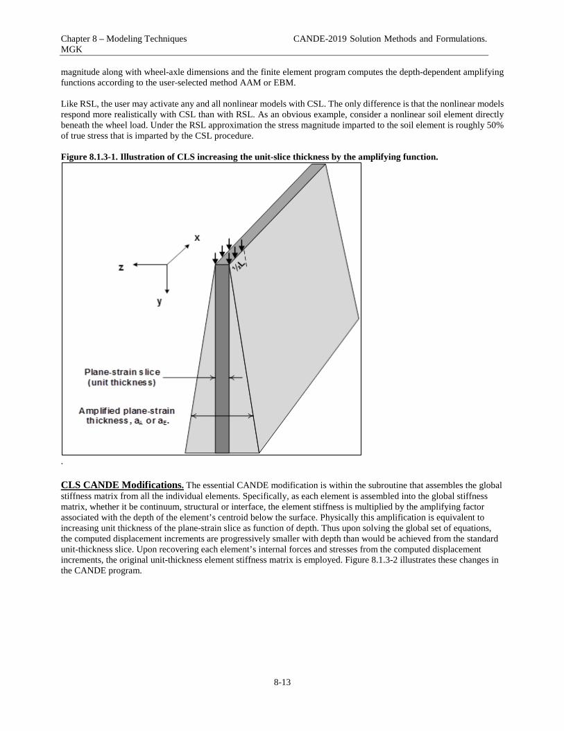
Chapter 8 – Modeling Techniques CANDE-2019 Solution Methods and Formulations. MGK
8-13
magnitude along with wheel-axle dimensions and the finite element program computes the depth-dependent amplifying functions according to the user-selected method AAM or EBM. Like RSL, the user may activate any and all nonlinear models with CSL. The only difference is that the nonlinear models respond more realistically with CSL than with RSL. As an obvious example, consider a nonlinear soil element directly beneath the wheel load. Under the RSL approximation the stress magnitude imparted to the soil element is roughly 50% of true stress that is imparted by the CSL procedure. Figure 8.1.3-1. Illustration of CLS increasing the unit-slice thickness by the amplifying function.
.
CLS CANDE Modifications. The essential CANDE modification is within the subroutine that assembles the global stiffness matrix from all the individual elements. Specifically, as each element is assembled into the global stiffness matrix, whether it be continuum, structural or interface, the element stiffness is multiplied by the amplifying factor associated with the depth of the element’s centroid below the surface. Physically this amplification is equivalent to increasing unit thickness of the plane-strain slice as function of depth. Thus upon solving the global set of equations, the computed displacement increments are progressively smaller with depth than would be achieved from the standard unit-thickness slice. Upon recovering each element’s internal forces and stresses from the computed displacement increments, the original unit-thickness element stiffness matrix is employed. Figure 8.1.3-2 illustrates these changes in the CANDE program.

Chapter 8 – Modeling Techniques CANDE-2019 Solution Methods and Formulations. MGK
8-14
Figure 8.1.3-2. CANDE flow chart for implementing continuous load scaling - CLS (red boxes).
Standard Input (Level 3) A-1. Key Commands A-2. Pipe Type B-x. Culvert Properties C-1. PREP line C-2. Control variables C-2a. New input line C-3. Nodal data C-4. Element data C-5. Boundary conditions D-x. Material data E-x. LRFD Load factors
Load Step Loop:i = 1 to N-steps
Construct Element Stiffness • kn = Element stiffness matrix• n = element number
Nonlinear Convergence?
Update responsesPrint Results
Next load step
Add input line C-2a for scaling data.If Iscale =1 or 2, user supplied data:• Live-step-start (default = last step)• Live-step-stop (default = last step)• Patch Length L (default = 10")• Patch Width W (default = 20")• Wheel spacing on axle (default = 72")--------------------------------------------------------Create Element Scaling Amplifiers.Loop through all elements to create and save amplifying value based on element’s depth below surface:aE(n) = EBM amplifier (if Islave = 1)aA(n) = AAM amplifier (if Islave = 2) n = element number
Add “Iscale” to control variables:• Iscale = 0, scaling not requested.• Iscale = 1, EBM (Elasticity-Based) • Iscale = 2, AAM (AASHTO-Ad hoc)
Yes No
Yes
No
Solve Equations KΔu = ΔP• ΔP = External load vector• Δu = incremental unknowns
Recover Element Forces• Fn = knΔu• Note, kn not amplified
αn = 1.0
Iscale > 0 ?And
L-start ≤ i ≤ L-stop ?
Assemble Global StiffnessK ← αnkn
αn = aE(n) if Iscale=1αn = aA(n) if Iscale=2

Chapter 8 – Modeling Techniques CANDE-2019 Solution Methods and Formulations. MGK
8-15
The red boxes in the above flow chart show the additional programming logic to incorporate the CLS procedure into the CANDE program and are discussed below.
1. The first red box introduces a new control parameter called “Iscale”, which must be input with a non-zero
value if the user wishes to activate CLS. Otherwise, continuous scaling is not performed and the traditional RSL may be employed. Choosing Iscale = 1, activates the elasticity-based method (EBM) and Iscale = 2 activates the AASHTO Ad hoc method (AAM).
2. Assuming that Iscale > 0, the 2nd red box defines input to be supplied by the user. Specifically, the user identifies the starting and ending load step numbers that correlates with the live loads to be continuously scaled. Also the wheel’s footprint dimensions must be defined as well as the spacing between wheels on the axle. Lastly, a node on the travel surface is required to establish the surface elevation. The above data is used to compute and save the amplifying value aA(n) or aE(n) for each element n, dependent on depth of the element’s centroid. One or two-wheel amplifiers are computed based on the element’s depth and Hint.
3. During the assembly of the global stiffness matrix each element stiffness matrix is multiplied by the element’s individual amplifying value providing that CLS is turned on (Iscale > 0) and the load step counter is within the range of the declared live load steps.
It is worth emphasizing that CLS does not change the algorithms for recovery of element forces or the nonlinear solution strategy. Indeed, it is important to use the original element stiffness (unit thickness) in order to properly compute the reduced internal forces resulting from the reduced displacements. Finally, a programming subtlety not shown in Figure 7 is required for special elements based on constraint equations, such as CANDE’s interface and link elements. For these specialized elements the primary unknowns are intra-node forces, and the elements’ right-hand-side “load vector” may contain non-zero displacement gaps. In these cases, the element load vector must also be scaled with same amplification factor as the element stiffness matrix in order to impose the correct displacement gaps.
8.1.4 Compare RSL and CLS in Free Field In this section RSL and CLS solutions are compared with the exact 3D solution for a patch load on an elastic half space as previously portrayed. The Figure 8.1.4-1 shows the symmetric 2D finite element mesh used by CANDE to simulate the 3D elastic half space configuration. Patch pressure is 1 psi with footprint dimensions L = 10 inches modeled explicitly in-plane, and W0 = 20 inches represented implicitly in RSL and CSL procedures. Elastic properties for the homogenous soil material are nominally taken as Young’s modulus = 1000 psi and Poisson ratio = 0.3 Figure 8.1.4-2 displays the peak soil stress versus soil depth as predicted by the four CANDE 2D models and the exact 3D elasticity solution. The dashed lines are RSL solutions for AAM and EBM based on an arbitrary choice H = 24 inches. The exact 3D solution is shown by the curve with green dots and the CSL solutions are shown by the solid red and black curves for EBM and AAM, respectively

Chapter 8 – Modeling Techniques CANDE-2019 Solution Methods and Formulations. MGK
8-16
Figure 8.1.4-1 CANDE mesh for RSL and CSL simulation of 3D half space.
Figure 8.1.4-2. Peak soil stress versus soil depth for exact 3D and CANDE 2D methods.
Center-line symmetry
5"
1 psi pressure on half-patch length
100"
100"HomogeousPlane-strain Slice
Chapter 8 – Modeling Techniques CANDE-2019 Solution Methods and Formulations. MGK
8-17
The following observations and insights are in reference to the above figure.
• The correlation between exact 3D and CANDE CLS-EBM solutions is amazingly close over the entire range of soil depths. Moreover, the close correlation is not limited to peak vertical stresses, but extends to all states of stress throughout the elastic half space.
• At the surface (y = 0), vertical soil stress should equal the applied patch pressure (1psi), which is correctly predicted by the 3D elasticity and the CANDE CLS-EBM and CLS-AAM solutions. However, the CLS-AAM solution tracks below the exact solution as soil depth increases.
• As expected, RSL-AAM and RSL-EBM solutions under-predict the surface soil stress in direct proportion to the reduction factors; rA-1 = 0.421 and rE-1 = 0.546, respectively. At soil depth y = 24 inches, the RSL-EBM solution intersects the 3D solution and then tracks above it for deeper soil depths. Similar behavior is observed for the RSL-AAM solution.
• To verify the above results are independent of the elastic properties assigned to the homogenous half space, additional CANDE solutions were obtained using a wide range of choices for Young’s modulus and Poisson ratio. The CANDE solutions were the same as shown above for all variations of elastic soil properties.
The major finding from the above free-field study is that the CANDE CLS-EBM solution provides a very close match to the exact 3D elasticity solution. Additional studies published in the Transportation Research Record (Reference 31) compare 3D finite element solutions of buried culverts under live loads with the RSL and CLS CANDE solutions. Again, it is shown that CLS-EBM is the most accurate method to simulate live loads and is the recommended procedure to use with CANDE.
8.1.5 Live Load 3D Stiffness Effects (RSL and CLS) The so-called 3D stiffness effect (3DSE) is not well understood by the culvert engineering community mainly because the current AASHTO LRFD Specification 4.6.2.10 does not identify the special distribution width as a 3D stiffness effect. Rather, AASHTO simply presents a special live-load distribution width for reinforced concrete box and arch culverts in shallow burial conditions without explaining the associated physics. For completeness, the AASHTO special distribution width equation is reviewed below followed by a discussion on the physical meaning behind the equation. Lastly, the 3D stiffness effect is generalized and incorporated into 2D analysis using RSL and CLS procedures. AASHTO Review. AASHTO Section 4.6.2.10 specifies a special longitudinal distribution width for reinforced concrete box and arch culverts when H < 2 feet of fill as shown below,
AxleE = 96" +1.44 Span ∗ ≤ 2 lay-lengths for precast culverts Equation 8.1-16a
where, EAxle = Longitudinal distribution width for axle load (inches) Span = Reinforced concrete box or arch span (feet) To be consistent with the AAM 1-wheel-load spreading width, Equation 8.1-16a may be equivalently written for 1-wheel loading as,
Wheel
1
2E = (96" +1.44 Span) ∗ ≤ 1 lay-length for precast culverts Equation 8.1-16b
where, EWheel = Longitudinal distribution width for one wheel load (inches) Span = Reinforced concrete box or arch span (feet)

Chapter 8 – Modeling Techniques CANDE-2019 Solution Methods and Formulations. MGK
8-18
Dividing the truck’s axle load by EAxle or the truck’s wheel load by EWheel produces the same line-load intensity that AASHTO recommends for 2D analysis of r/c boxes and arches when H < 2 feet. However, for H ≥ 2 feet, AASHTO specifies the traditional AAM soil-spreading line load, i.e., wheel-load divided by (W0+1.15H). As a consequence, the line-load magnitude has a jump increase at H = 2’ because EWheel is significantly larger than the traditional AAM soil-spreading distribution width at H = 2 feet. This begs many questions. First and foremost, “Where does “Equation 8.1-16” come from?”. Equation 8.1-16 originates from the PennDOT sponsored study conducted in 2004 by SGH (Reference 32). The study was motivated by PennDOT’s observation that shallow buried r/c box culverts appear to be much more robust under live loading than indicated by traditional 2D analysis. To pursue this question, the PennDOT study used NASTRAN to obtain 3D finite element solutions of reinforced concrete box culverts subject to HS20 truck loads. Overall, 31 linear box and slab model configurations were analyzed with spans ranging from 8 to 24 feet and cover heights from zero to two feet. By comparing the 3D solutions to 2D solutions, the PennDOT study proposed the special distribution width given by Equation 8.1-16 so that the 2D and 3D solutions predicted comparable results for the controlling internal forces. AASHTO adopted the recommendation from the PennDOT study and incorporated the special distribution width into Section 4.6.2.10 of the LRFD Bridge Specifications. However, the AASHTO commentaries do not provide a discussion on the physical meaning of this special distribution width. Clearly, the special distribution width is not related to load spreading through the soil because at the surface EWheel is much larger than the actual wheel width. Physical Insights. The special distribution width (EWheel) compensates for the additional stiffness observed in the 3D world but is not realized in the 2D world. Said another way, the 2D model does not include the longitudinal bending and twisting stiffnesses that actually occurs when the longitudinal load width is relatively short compared to the culvert’s length. Accordingly, when the 2D model under-represents the actual stiffness, the 2D line load intensity is reduced by the W0/EWheel so that worst-case structural response predicted by the stiffer 3D models agree with the 2D models. The above concepts are clarified in the following paragraphs which are adapted from Reference 33. To simplify the understanding of 3DSE, consider two identical flat plates with span and length dimensions similar to the top slab of a precast box culvert. The plates are fixed along the left and right sides and free to deflect at the ends as shown in Figure 8.1..5-1. The left plate has a longitudinal line load of magnitude p (force/length) extending the entire length of the plate, and the right plate is loaded with same line load magnitude p but terminated at an arbitrary footprint width W, measured from the front end. In short, the left plate model is referred to as 2D strip loading and the right plate model as 3D footprint loading. Figure 8.1.5-1. Rectangular plate model with partial and full line-load widths W with magnitude p (lbs./inch).

Chapter 8 – Modeling Techniques CANDE-2019 Solution Methods and Formulations. MGK
8-19
The red lines in the above figure illustrate the deformation patterns where the symbol Δ refers to the vertical deflection along the centerline’s z axis. For the 2D strip loading, the plate deforms uniformly in one-way bending without variation along the z-axis with a constant centerline displacement Δmax. Due to one-way plate bending, the deformed shape in the x-y plane is exactly equivalent to a fixed-end beam whose cross-section is a unit slice of the plate. Thus, the 2D resistance to deformation is supplied solely by the plate’s in-plsne bending stiffness about the z-axis. In contrast, the 3D footprint loading produces a nonuniform deformed shape dependent on the footprint width W. The peak displacement Δ(W) occurs on the plate centerline at z = 0 and diminishes along the z-axis due to resisting longitudinal and twisting moments as explained by the following thought experiment. Imagine that the right plate is severed into two separate segments along the plane z = W so that the forward segment contains the 3D footprint load and the rear segment is load free. Since the two plate segments are severed, no forces or moments are transmitted between the segments. Hence, the front segment deforms exactly like the 2D strip-load with uniform displacement Δmax, and the rear segment is undeformed. Based on this thought experiment, we conclude that the unloaded portion of the intact plate provides additional bending and twisting stiffnesses that are not activated by the 2D strip load. This phenomenon is the meaning behind the term “3D stiffness effects” or 3DSE. Plate Model Solution. Deeper insight into the plate’s structural behavior is provided by a closed-form Ritz solution of the plate model developed by the author. The Ritz displacement solution is the product of beam-theory displacement function Δ(x) times the dimensionless function f(z) for 0 ≤ z ≤ l. The arguments of f include span-to-length ratio s/l, the footprint ratio W/l and the orthotropic bending-stiffness ratio Dx/Dz. The Ritz solution for centerline deflection is functionally espessed by Equation 8.1-17 assuming isotropic bending stiffness, Dx = Dz = D.
max( ) ( , , )z W sz fl l l
∆ = ∆ Equation 8.1-17
Δmax = maximum 2D centerline displacement (same as beam theory for unit slice) p = line-load intensity (force per unit length) s = span of plate l = length of plate D = EI/(1-ν2) = isotropic plate bending stiffness per unit width about x or z axis. f = dimensionless longitudinal function, range 0 ≤ f ≤ 1. W/l = percentage of load footprint over plate length, 0 ≤ W/l ≤ 1. The dimensionless function f is not written explicitly because it is a cumbersome expression that provides little insight without visually plotting the behavior for various footprint widths, to be shown in the next section. However for the special case W=l (i.e., 2D strip load), then the function f(z) ≡1 for all z so that the above equation simplifies to the uniform one-way beam bending with maximum displacement shown below,
3
192max( ) sz pD
∆ = ∆ = Equation 8.1-18
Results from the plate model solution are used to define two important parameters that define the load-width range of 3DSE influence. These two important parameters are called Wcritical and Wmin. Introducing Wcritical. The critical distribution width called Wcritical is succinctly defined as follows. Wcritical is the minimum longitudinal footprint width that produces a peak 3D structural response in the controlling transverse section that is equal to the uniform 2D structural response. Accordingly, when W ≥ Wcritical, 3DSE no longer has an impact on the 2D solution, rather only standard load spreading methods are required to adjust the 2D analysis. However. when W < Wcritical, the benefits of 3DSE should be taken into account to correct the 2D analysis. Thus, Wcritical is the load width beyond which 2D solutions no longer benefit from 3DSE as illustrated next with plots of the plate model. Figure 1.8.5-2 shows centerline displacement profiles Δ(z)/Δmax for three increasing sizes of 3D footprints; W1 < Wcritical, W2 = Wcritical, and W3 > Wcritical. Also shown is the uniform maximum 2D displacement profile when W = l. Keep in mind that all footprint widths are directly impinging on the plate surface with the same line-load intensity p acting over each width. Therefore, the successive curves may be interpreted as increasing load widths due to longitudinal load spreading; however, the load intensity p is held constant.

Chapter 8 – Modeling Techniques CANDE-2019 Solution Methods and Formulations. MGK
8-20
Figure 8.1.5-2. Deflection profiles (symmetric half) for four key choices of W.
As previously defined and implied in the above figure, Wcritical is the minimum distribution width producing a peak 3D displacement at z = 0 that is equal to the uniform maximum 2D displacement, ΔMax. Wcritical is determined by forming the displacement ratio shown below and incrementally increasing the value of W until the ratio is equal to 1.
criticax
lMa
W = minimum W sΔ(W)
uch thatΔ
= 1 Equation 8.1-19
There is nothing magic about peak dispacement because any orther key structural response (e.g., maximum positive moment, maximum negative moment or peak shear) could be used in the above equation to produce the same value for Wcritical. Note that Wcritical is a physical property of the slab (culvert) irrespective of the soil or burial depth. Moreover, since Wcritical is determined from ratio as shown above, Wcritical is not influenced by linear plate parameters such as plate stiffness because these parameters cancel out in the ratio. For an isotropic plate, Wcritical is only dependent on span and length. Once Wcritical is known for a class of culverts, it is used in 2D analysis to define the transition soil depth, denoting the end of 3DSE benefits and the start of pure load spreading. The zone above the transition soil depth is where 3DSE effective distribution width becomes significantly more pronounced than the load spreading width. Indeed, for H = 0 (zero soil cover), the effective 3DSE distribution width is called Wmin and is defined in the following section. Introducing Wmin. Wmin is the minimum 3DSE distribution width associated with the minimum possible load width W0 acting on the culvert. Like Wcritical, Wmin is a culvert property and is determined with aid of 3D solutions based on the worst-case 3D-to-2D structural response ratio as will be illustrated with the aid of the plate model Ritz solutions. Figure 8.1.5-3 shows 3D-to-2D response ratios as function of load width W for 3 key structural responses in the transverse plane at z = 0; deflection at center, moment at center and shear at edge. Initially these key response ratios form distict nonlinear curves with steep slopes that gradually decreases to zero as W approaches Wcritical. When W ≥ Wcitical, all 3D-to-2D ratios are equal to 1.0, indicating the entire transverse section at z = 0 is distressed exactly like the 2D slice.

Chapter 8 – Modeling Techniques CANDE-2019 Solution Methods and Formulations. MGK
8-21
On the other hand, when W < Wcritical it is evident that 3D stiffness effects reduce the key structural responses in the 3D plate in comparison to the more-distressed 2D slice with sane load intensity p. However, the 3DSE benefit is not the same for each key structural response; hence the highest curve (worst case) is used to conservatively determine Wmin for load width W0. This procedure the is illustrated in the figure below. Figure 8.1.5-3. Key 3D-to2D structural response ratios versus load widths from 0 to L acting on plate.
In the above illustration, the controlling key response ratio is “cemter moment” whose value ≈ 0.53 for the minimum load width W0. Therefore, to reduce the 2D solution to replicate the worst-case 3D solution, the 2D surface pressure p is reduced with the reduction factor, r = W0/Wmin where the minimum 3DSE distribution width is determined by extrapolating as shown above, or simply by the proportionality expression,
0min
WW =
Controlling 3D/2D ratio Equation 8.1-20
To summarize, the proposed 3DSE distribution width starts at Wmin for load width W0 (H = 0) and expands to Wcritical at the transition soil depth HTrans where load spreading W(HTran) is equal to Wcritical. As a side comment, it interesting to note that if if all the key structural response ratios increased linearly from W = 0 to Wcritical as indicated by the dashed line in the above figure, then the 3DSE distribution width would remain constant at Wcritical; however, this is not the case.

Chapter 8 – Modeling Techniques CANDE-2019 Solution Methods and Formulations. MGK
8-22
Complete details for implementing 3DSE into the improved RSL and CLS procedures are presented in the next two sections. To this end, Wmin and Wcritical are viewed as known quantities for the particul class of culverts being analysed. The final section discusses the current and future status of quantifying Wmin and Wcritical. Improved RSL Procedure accounting for 3DSE. Recall that the traditional RSL procedure for “load spreading only” is summarized in Section 8.1.2 for both AAM and EBM load spreading theories. The improved RSL procedure presented here melds 3DSE with load spreading in a consistent and seamless manner based on Wmin and Wcritical. Figure 8.1.5-4 illustrates the improved procedure by showing the longitudinal view of two identical culverts, one representing shallow burial at depth H1 and the other representing deeper burial at depth H2. A wheel load with line intensity p0 is applied to the surface. The figure’s red lines define the special 3DSE distribution width denoted as W3DSE(H) that linearly increases from Wmin on the surface to Wcritical at the transition depth (H = HTrans), Thus the 3DSE distribution width is given by,
3DSE min critical minTrans
HW (H) = W + (W -W )H
Equation 8.1-21
Shown with solid green lines is the load-spreading distribution width W(H) representing the selected load spreading theory such as AAM or EBM as previously described. The red and green distribution widths are equal at the transition soil depth HTrans where W(HTrans) = Wcritical, thereby ensuring continuity from the 3DSE zone to the load-spreading zone. FIGURE 8.1.5-4 Longitudinal view of shallow and deeply buried culverts for improved RSL analysis.

Chapter 8 – Modeling Techniques CANDE-2019 Solution Methods and Formulations. MGK
8-23
The RSL procedure for 2D analysis simply requires determining a reduction factor for the surface line load that is dependent on a selected soil depth H, usually taken as cover over crown. For example, culvert #1 in the above figure with crown cover H1 is governed by the distribution width W3DSE(H1), whereas culvert #2 with crown cover H2 is governed by W(H2). In short, the reduction factor for the improved RSL method for any particular choice of H is given by the alternatives in the equations below as governed by the transition depth HTrans.
0 3DSE Trans
0 Trans
W /W (H) if H < Hr(H) =
W /W(H) if H H→
→ ≥ Equation 8.1-22
Note that the load spreading width W(H) is always taken as the load spreading width beneath one wheel for all depths H. Thus, if H is greater than the 2-wheel interaction depth, then W(H) is taken as one-half of the combined two-wheel footprint width. It is understood that Wmin and Wcritical are determined from 3D analysis accounting for full axle loading. It is informative to consider the physical soil pressure acting upon the crowns of culvert #1 and culvert #2. The bottom culvert experiences a uniform reduced pressure distribution between the solid green lines. In contrast, the top culvert only experiences actual soil pressure between the dashed green lines. The additional distribution width to the solid red lines artificially increases the reduction factor to account for actual 3DSE behavior that is invisible in a 2D unit slice model. These incongruities do not occur with the CLS procedure. presented next. Improved CLS Procedure accounting for 3DSE Recall that the CLS procedure for “load spreading only” is summarized in Section 8.1.3 for both AAM and EBM load spreading theories. The improved CLS procedure as presented here incorporates the additional 3DSE zone directly into the culvert element 2D stiffness matrices while at the same time simulating load spreading throughout the 2D soil-structure slice in a continuous manner. To emphasize the continuous nature of CLS versus RSL, the depth variable is denoted as y instead of H (specifird depths) as shown in the figure below. FIGURE 8.1.5-4 Longitudinal view of a buried culvert for the improved CLS analysis procedure.

Chapter 8 – Modeling Techniques CANDE-2019 Solution Methods and Formulations. MGK
8-24
The above figure shows the longitudinal view of a culvert, wherein the solid red lines define the special 3DSE distribution width denoted as W3DSE(y) that linearly increases from Wmin on the surface (y = 0) to Wcritical at the transition depth (y = HTrans). Shown with solid green lines is the load spreading distribution width W(y) representing the selected load spreading theory such as AAM or EBM as previously described. The red and green distribution widths are equal at the transition soil depth HTrams where W(HTrans) = Wcritical, thereby ensuring continuity from the 3DSE zone to the load-spreading zone. CLS mimics reality by amplifying the unit thickness (stiffness) of every soil by the load-spreading amplification ratio W(y)/W0. To account for 3DSE, which is strictly a property of the culvert, the superiority of CLS procedure becomes evident. Specifically, the stiffness of culvert elements above the transition depth HTrams are amplified by the 3DSE ratio W3DSE(y)/W0, whereas the culvert element stiffnesses below HTrans are amplified for load spreading only, W(y)/W0. To summarize, the CLS amplification factors for are not only dependent on each element’s depth below the surface, but also dependent on the type of element, soil or structure, as summarized below. For each soil element the amplification factor is given by,
0
W(y)a(y) = W
where y = soil element’s depth. Equation 8.1-23a
And for each culvert element the amplification is also dependent on HTrans and is given by,
3DSE 0 Trans
0 Trans
W (y)/W if y < Ha(y) =
W(y)/W if y H→
→ ≥ where y = culvert element depth. Equation 8.1-23b
inwhich, 3DSE min critical minTrans
W (y) = W + (W -W )H
y Equation 8.1-23c
To remain consistant for all measures of load and distribution widths, W(y) is defined as the soil-spreading width (AAM or EBM) beneath one wheel. Therefore, W(y) is taken as one-half of the combined two-wheel footprint width when y is greater than the 2-wheel interaction depth, Hint. Accordingly, Wmin and Wcritical are culvert properties representing 3DSE widths associated with one wheel; however, the size of Wmin and Wcritical is influenced from two-wheel axle loading. This concept is fully explained in Reference 33 by describing how 3D FEM programs should be used to determine Wmin and Wcritical for any class of culverts. Lastly, recall that Section 8.1.3 provided a detailed flow-chart on modifying the CANDE program to perform CLS for soil-load-spreading. Inspecting this flow chart, it should be evident that only small changes in the logic are needed to include the 3DSE amplification factor in accordance with Equation 8.1-22b. Accordingly, the revised CANDE-2019 program now includes the CLS-3DSE option and is available at the CANDE website, CandeForCulverts.com. Refer to the CANDE-2019 User Manual, Level 3, line C-2 to actvate the CLS options. Not too surprisingly, preliminary live-load studies comparing RSL versus CLS predictions for r/c box and arch culverts indicate CLS solutions are more accurate. Current and future determination of Wmin and Wcritical. Currently, the only “sanctioned equation” for quantifying Wmin is the AASHTO special distribution width for r/c boxes and arches, denoted as EWheel in Equation 8.1-16b. It can be rigourously proven that the calculation procedure for EWheel is exactly equivaent to Wmin as defined by Equation 8.1-20. AASHTO does not currently employ a parameter equivalent to Wcrtical. Rather, AASHTO assumes the 3DSE distribution width remains constant and equal to Wmin. Therefore, to mimic current AASHTO using the new improved RSL and CLS procedures, Wcritical is set equal to Wcritical and quantified by the following AASHTO equation.
min critical1
2= 96" +1.44*Span(ft)] 1 lay length (inches)W = W [ ≤ Equation 8.1-24

Chapter 8 – Modeling Techniques CANDE-2019 Solution Methods and Formulations. MGK
8-25
The consequence of choosing Wcritical = Wmin instead of a realistic larger vaule is that the 3DSE distribution widths are shorter than reality. Hence, this is a conservative error, which may be acceptable for design purposes but not desireable for load rating if false no-go rating factors are predicted. In the very near future, NCHRP project 15-54 will submit a final report with recommendations to AASHTO for improving 2D analysis procedures for load rating. It is fairly certain that the new-improved RSL and CLS procedures using Wmin and Wcritical will be compatible with the NCHRP 15-54 recommendations. It is anticipated that the following general recommendations will be made to improve AASHTO specifications:
• Consistantly define all distribution widths relative to one wheel to avoid blunders in transitioning from axle loads to wheel loads. (Of course, the size of 3DSE distribution widths are calculated with full axle loading.)
• Ensure smooth transitions from 3DSE to soil load spreading at the proper transition soil depth. (Eliminate the arbitrary and discontinuous transition depth at 2 feet)
• Improved equations defining Wmin and Wcritical for r/c box culverts that include the influence of span and lay length. (The original PennDOT study did not investigate the important effect of box lay length).
• New equations defining Wmin and Wcritical for r/c arches as a function of span and lay length. (The original PennDOT study did not investigate arch shapes, arches were simply assumed to behave like a box.)
Undoubtedly, future research efforts will continue to investigate the benefits of 3DSE for other culvert materials and shapes beyond r/c boxes and arches. To this end, Reference 33 provides a comprehensive step-by-step procedure for using 3D FEM prograns to develop equations for Wmin and Wcritical as function of gross geometry for each class culverts. The beauty of the CANDE-2019 program is that it can account for 3DSE benefits for any class of culverts providing there exists AASHTO sanctioned equations for Wmin and Wcritical for the culvert being analysed. For the RSL method of analysis, the user determines the reduction factor from Equation 8.1-21 and reduces the service live load accordingly. For the CLS method of analysis, the user inputs the actual service live load as well as values for Wmin and Wcritical from which the CANDE program automatically amplifies the culvert stiffness in accordance with Equation 8.1-23.

Chapter 8 – Modeling Techniques CANDE-2019 Solution Methods and Formulations. MGK
8-26
8.2 Pipe Group Connections and Combinations Finite element models utilizing multiple pipe groups is a new feature in CANDE-2019 that offers many modeling capabilities that were not available in previous versions of CANDE. Discussed below are several techniques for combing pipe groups with each other and soil elements to achieve various desired objectives. Topics include connection modeling (fixed, pinned, and roller), long-span stiffeners, culvert rehabilitation with liners, and other pipe group combinations.
8.2.1 Connections among element types A pipe group is a connected sequence of beam-column elements joined head-to-toe at common nodes and tracing an arbitrary curvilinear path in x-y space. Each beam-column node has three degrees of freedom, x-displacement, y-displacement and a rotation. Continuum elements (triangle or quadrilateral) only have two degrees of freedom per node, x-displacement and y-displacement. When two or more pipe groups are connected to a common node the connection is called fixed, meaning moment continuity is preserved at the junction node. On the other hand, when a pipe group is attached to a continuum element the connection is called pinned, meaning the moment at the junction node is zero. These fundamental connections, representing the default conditions, are illustrated in the figure below. Figure 8.2.1-1 Connections made by sharing common node at junction.
If it is desired to simulate a pinned or roller connection between two pipe groups such as pipe group #1 and pipe group # 2 in the above figure, then an interface element must be inserted at the junction of the two the two pipe groups. An interface element joins two independent nodes, initially assigned to the same x-y coordinate location, as a pinned connection, friction connection or roller connection depending on the properties assigned to the interface element. Figure 8.2.1-2 illustrates an interface element joining pipe group # 1to pipe group # 2 including the third interface node whose degrees of freedom are the interface forces required to enforce the desired connection.

Chapter 8 – Modeling Techniques CANDE-2019 Solution Methods and Formulations. MGK
8-27
Figure 8.2.1-2 Techniques to change connection conditions.
The assigned interface properties required to achieve various connection conditions are listed in the table below wherein the value 106 means a very large number such that frictional slippage or tensile rupture cannot occur. Table 8.2.1-1 Interface property values to simulate various connection conditions
Desired Connection Type
Interface properties
Friction coefficient (μ)
Tensile breaking force (lbs/inch)
Pinned
106
106
Friction (no tensile separation)
0.3 (typical)
106
Friction (tensile separation)
0.3 (typical)
0.0
Roller (no tensile separation)
0.0
106
Roller (tensile separation)
0.0
0.0
Shown on the right side of Figure 8.2.1-2 is a modeling technique to simulate a fixed connection between a pipe group and a concrete footing (continuum elements). Here a beam-column element is added to the pipe group and imbedded in the concrete, mimicking reality.
8.2.2 Stiffeners and culvert rehabilitation with parallel pipe groups When two pipe groups share the same set of nodes, referred to as parallel pipe groups, it is evident that both groups experience identical deformations (displacements and rotations) because both pipe groups are attached to the same nodes. The combined stiffness is additive, exactly like two parallel springs with individual stiffnesses k1 and k2 have a combined stiffness equal to k1 + k2. Even though parallel pipe groups experience identical deformations, the resulting internal forces (moment, thrust and shear) and stresses in one group may differ substantially from the other group, depending on individual stiffness properties of each group. Many types of culvert stiffeners can be modeled with parallel pipe groups with one pipe-group modeling the culvert and the second pipe-group modeling the stiffener. As noted above, a stiffener that is modeled as a parallel pipe group provides an additive stiffness to the culvert without additional increase in bending stiffness from composite action. To achieve composite action the stiffener must be integrally attached to the culvert including complete shear bonding like a continuously welded built-up cross sections. Culvert sections that are truly stiffened in a composite manner can be
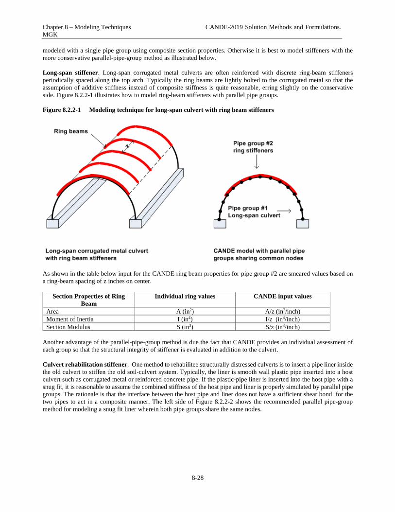
Chapter 8 – Modeling Techniques CANDE-2019 Solution Methods and Formulations. MGK
8-28
modeled with a single pipe group using composite section properties. Otherwise it is best to model stiffeners with the more conservative parallel-pipe-group method as illustrated below. Long-span stiffener. Long-span corrugated metal culverts are often reinforced with discrete ring-beam stiffeners periodically spaced along the top arch. Typically the ring beams are lightly bolted to the corrugated metal so that the assumption of additive stiffness instead of composite stiffness is quite reasonable, erring slightly on the conservative side. Figure 8.2.2-1 illustrates how to model ring-beam stiffeners with parallel pipe groups. Figure 8.2.2-1 Modeling technique for long-span culvert with ring beam stiffeners
As shown in the table below input for the CANDE ring beam properties for pipe group #2 are smeared values based on a ring-beam spacing of z inches on center.
Section Properties of Ring Beam
Individual ring values CANDE input values
Area A (in2) A/z (in2/inch) Moment of Inertia I (in4) I/z (in4/inch) Section Modulus S (in3) S/z (in3/inch)
Another advantage of the parallel-pipe-group method is due the fact that CANDE provides an individual assessment of each group so that the structural integrity of stiffener is evaluated in addition to the culvert. Culvert rehabilitation stiffener. One method to rehabilitee structurally distressed culverts is to insert a pipe liner inside the old culvert to stiffen the old soil-culvert system. Typically, the liner is smooth wall plastic pipe inserted into a host culvert such as corrugated metal or reinforced concrete pipe. If the plastic-pipe liner is inserted into the host pipe with a snug fit, it is reasonable to assume the combined stiffness of the host pipe and liner is properly simulated by parallel pipe groups. The rationale is that the interface between the host pipe and liner does not have a sufficient shear bond for the two pipes to act in a composite manner. The left side of Figure 8.2.2-2 shows the recommended parallel pipe-group method for modeling a snug fit liner wherein both pipe groups share the same nodes.

Chapter 8 – Modeling Techniques CANDE-2019 Solution Methods and Formulations. MGK
8-29
Figure 8.2.2-2 Modeling techniques for culvert rehabilitation with liners
The right side of the above figure shows an alternative rehabilitation method in which the outside diameter of the liner is several inches smaller than the inside diameter of the host pipe thereby creating an annular space that is filled with grout. In this case the combined stiffness of liner, host pipe and grout is significantly greater than the snug fit condition using parallel pipe groups. As illustrated in the figure, an accurate simulation is achieved by assigning the liner an independent set of nodes tracing its smaller diameter and modeling the grout with continuum elements. If the grout elements are assigned common nodes with the liner pipe and with the host pipe, the net effect is a composite bending stiffness that may be overly optimistic if the grout is not securely bonded both pipes. Therefore, a more conservative approach would be to assign independent node numbers to the grout elements and use frictional interface elements to connect the grout nodes to the pipe nodes, allowing relative slip along the pipe-grout boundaries.
8.2.3 Illustrations of pipe group combinations In addition to the pipe group connections and combinations discussed above, additional pipe-group applications are illustrated in the Figure 8.2.2-3.

Chapter 8 – Modeling Techniques CANDE-2019 Solution Methods and Formulations. MGK
8-30
Figure 8.2.3-1 Illustrations of multiple pipe group applications
The above illustrations are intended to demonstrate the wide variety of modeling options that are possible with CANDE’s multiple pipe-type capability. For example, the reinforced earth application (last figure) implies that pipe groups can be used to simulate soil reinforcement strips. If interface elements are inserted along these pipe groups, the model is capable of determining the ultimate pullout strength of the soil reinforcement.

Chapter 8 – Modeling Techniques CANDE-2019 Solution Methods and Formulations. MGK
8-31
8.3 Construction Increments Incremental construction is the physical process of placing and compacting soil layers, one lift at a time, below, alongside and above the culvert as the installation is constructed. Analytically this is achieved by adding incremental solutions from successive finite element configurations, where each new configuration contains additional soil elements (and/or structural elements) that mimics the real-world buildup of the soil-structure system, one load step at a time. The terms “load step” and “construction increment” are closely related terms and are often used interchangeably, however they have slightly different meanings. Load step is an all-encompassing term referring to any incremental solution, which may or may not include a construction increment. For example a load step may only include boundary-condition loads without additional elements added to the system. A construction increment is a special kind of load step wherein additional elements are added to the global stiffness matrix usually representing an additional layer of soil. The body weight of added elements form the load increment associated with the load step along with any boundary loads such as soil compaction pressures, discussed subsequently.
8.3.1 Rules and insights for construction increments With the above understanding, construction increments are subject to the following rules. Each element is assigned a construction increment number, which corresponds to the load step number that the element stiffness matrix and load vector is assembled into the global system. Once an element stiffness enters the system it remains active for all subsequent load steps (there is no element death,except for link element). Of course, the element body-load vector is only applied during the load step corresponding to the element construction increment number; it is not reapplied on subsequent load steps. Similarly, surface pressure and/or point loads (i.e., force boundary conditions) are also assigned a particular construction increment number and are only applied during the corresponding load step. Likewise, displacement boundary conditions are applied during the load step they are specified and remain fixed for all subsequent load steps. In short, the rules simulate reality. Although the rules seem simple, it is easy to be fooled. For example, novices generally think that if all construction increments are linear elastic and no other nonlinearities are involved, then a structure built in several steps behaves no differently than a structure built as a monolith (all in one step). A simple example demonstrating this is not true is shown in the figure below. Figure 8.3.1-1 Illustration of two construction increments versus a single monolith
The figure illustrates that after the first construction increment is set in place with roller boundary conditions on the sidewalls, the body weight produces a uniform stress distribution properly aligned in the vertical direction as expected. However, when the second construction increment is set in place (sharing common nodes with the first construction increment), some of the second construction increment’s body weight is transferred to the first construction increment’s stiffness. Therefore, the resulting stress and strain distribution in the two-step system is not uniform and differs from the uniform stress distribution in the single monolith system shown on the right.

Chapter 8 – Modeling Techniques CANDE-2019 Solution Methods and Formulations. MGK
8-32
The specific point of this simple example is that the sequence of construction increments is important and influences the structural behavior of the final system. More generally, when developing a finite element model for a particular soil-structure system, the sequence of construction increments should be modeled as realistically as practical.
8.3.2 Techniques for initial construction increment All too often the first construction increment is not modeled properly, causing incorrect deformation in the structure due to the insitu soil model. Proper modeling techniques depend on whether the insitu soil is linear or nonlinear and the assignment of body weight as discussed below. Linear insitu soil. Generally insitu soil can be realistically modeled with a linear elastic soil model because the existing soil is pre-consolidation and/or recently unloaded from excavation. In this case, the initial construction increment may include the insitu soil, footing or bedding and the structure as illustrated in the example below. Figure 8.3.2-1 Initial configuration for an arch-trench installation with linear insitu soil
Only the arch should be assigned a non-zero body weight for this initial configuration. A common mistake made by novices is to also assign body weight to the insitu soil and footing, which causes these components to deform under their own weight and introduce fictitious distortions into the arch. Physically we know the insitu soil and footing are at rest under their own weight before the arch is attached to the footing, thus only the arch body weight cam cause deformations in the first load step. Nonlinear insitu soil. If it is desired to model the insitu soil with a nonlinear soil model like Duncan/Selig, then the arch should be eliminated from the initial configuration and introduced in the second construction increment. In this case we need to assign the actual body weight to the insitu soil because the soil stiffness is dependent on the stress state caused by the soil body weight, requiring iteration within the load step. Figure 8.3.2-2 illustrates the proper initial configuration when nonlinear soil model is used for insitu soil.

Chapter 8 – Modeling Techniques CANDE-2019 Solution Methods and Formulations. MGK
8-33
Figure 8.3.2-2 Initial configuration for an arch-trench installation with nonlinear insitu soil
If the arch were included in the initial configuration, it would experience fictitious distortions due to deformation of the insitu soil by self-weight. Now however, after the initial configuration has converged and the insitu soil and footing are at rest in a deformed state, the arch may be correctly assigned to the second construction increment.
8.3.3 Soil compaction and construction increments The last technique to be described is the modeling of soil compaction using the so-called squeeze layer method first introduced in Reference 18. The purpose of soil compaction is to densify soil after it is laid down in loose layers and then compacted to achieve a specified density usually stated in terms of AASHTO T-99 relative density. Compaction equipment ranging from hand-held compactors to large-tracked bulldozers is used to compress each soil layer by creating a temporary vertical pressure to compact the soil. As the soil is compressed vertically (squeezed), it tends to expand laterally due to the Poisson effect, which creates horizontal pressure on the sides of the culvert. These lateral pressures cause inward movement of the culvert sides and peaking at the culvert crown, that is, a reverse deformation pattern from that caused by overburden loading. Large culverts such as long-span corrugated metal structures often experience as much as 2 % crown peaking as a result of compacting soil layers between the footing and the crown. Compaction loads are beneficial not only in compacting the soil to achieve the desired soil stiffness properties but also in introducing reverse deformations and bending moments into the culvert, which provides the culvert with additional capacity to resist the opposite bending deformations that subsequently come from soil placed on top of the culvert. The squeeze layer technique is a simple modeling concept that simulates the effect of soil compaction and is applicable to both linear and nonlinear soil models. The concept is illustrated in Figure 8.3.3-1.

Chapter 8 – Modeling Techniques CANDE-2019 Solution Methods and Formulations. MGK
8-34
Figure 8.3.3-1 Squeeze-layer method for compaction loads on long-span culvert.

Chapter 8 – Modeling Techniques CANDE-2019 Solution Methods and Formulations. MGK
8-35
A point by point discussion of the above figure is provided below.
1. To start, a uniform compaction pressure representing the compaction equipment, typically on the order 5-psi pressure, is placed on the surface of the insitu soil at the level of the footing.
2. Next, the 2nd construction increment (first layer of backfill soil with body weight) is added to the system along
with another uniform compaction pressure applied to its top surface. At the same time, however, the first compaction pressure is removed by applying an equal but opposite compaction pressure to the bottom surface. These two opposing pressures squeeze the soil layer and increase the lateral pressure on the arch via the Poisson effect.
3. The intermediate construction increments 3rd, 4th and 5th are treated exactly like the 2nd construction increment
so that each layer is squeezed, increasing lateral pressure on the arch and inducing more peaking. Note that after the 5th load increment (or more generally, the increment before the crown-level increment) all the temporary compaction pressures have been removed except the compaction pressure on the surface of 5th construction increment.
4. The squeeze layer process is terminated with the 6th construction increment (i.e., crown-level increment). As the
6th construction increment is added to the system with its stiffness and body weight, the last remaining compaction pressure from the 5th construction is removed.
5. All the remaining construction increments, representing soil layers above the crown, are added in the normal
manner with body weight but without any compaction pressures. Examples of applying the squeeze layer technique and the behavior of long-span culverts can be found in References 18, 26 and 27. As an alternative to the squeeze layer technique, the plasticity Mohr-Coulomb and/or Duncan/Selig model with Katona modification may be used to model the backfill soil. In this case the compaction pressure is applied to the soil surface and then immediately removed in the next load step. Due to the permanent plastic deformation of these plasticity models, the unloading phase does not restore the soil layer to its original position and locked-in lateral forces are maintained on the structure.

Chapter 9 – References CANDE-2014 Solution Methods and Formulations
9-1
REFERENCES
1. CANDE: A Modern Approach for the Structural Design and Analysis of Buried Culverts, Federal Highway Administration Report No. FHWA-RD-77-5, October 1976, (Authors: M. G. Katona, J .M. Smith, R. S. Odello, and J. R. Allgood).
2. CANDE User and System Manuals, Federal Highway Administration Report No. FHWA-RD-77-6, October
1976, (Authors: M. G. Katona and J. M. Smith).
3. CANDE-1980: Box Culverts and Soil Models, Federal Highway Administration, Report No. FHWA-RD-172, May 1981 (Authors: M. G. Katona, P. D. Vittes, C. H. Lee, and H. T. Ho).
4. CANDE-89: Culvert Analysis and Design computer program – User Manual, Federal Highway Administration
Report No. FHWA-RD-89-169, June 1989. (Authors: S. C. Musser, M. G. Katona and E T. Selig).
5. Predicting Performance of Buried Conduits, Report No. FHWA/IN/JHRP-81/3, Joint FHWA and Indiana State Highway Commission, June 1982. (Authors; G.A. Leonards, T.H. Wu, and C.H. Juang)
6. AASHTO (2014), AASHTO LRFD Bridge Design Specifications, Current Edition, AASHTO, Washington, D.C.
7. Burns, J. Q., and R. M. Richard, “Attenuation of Stresses for Buried Cylinders,” In Proc., Symposium on Soil-
Structure Interaction, University of Arizona Engineering Research Laboratory, Tucson, 1964, pp. 378-392.
8. Herrmann, L. R., “User’s manual for plane strain incremental construction program,” Department of Civil Engineering, University of California, Davis, 1972.
9. Katona, M. G., and A. Y. Akl, “Analysis and Behavior of Buried Culverts with Slotted Joints,” Transportation
Research Record, No. 1008, 1985, pp. 22-32.
10. Katona, M. G., and A. Y. Akl, “Structural Design of Buried Culverts with Slotted Joints,” ASCE, Journal of Structural Engineering, January 1987.
11. Herrmann, L. R., “Efficiency evaluation of a two-dimensional incompatible finite element,” Journal of
Computers and Structures, vol 3, 1973, pp 1377-1395.
12. Katona, M. G., Minimum Cover Heights for Corrugated Plastic Pipe Under Vehicle Loading,” Transportation Research Record, No. 1288, 1990, pp. 127-135.
13. McGrath, T.J., I.D. Moore, E.T. Selig, M.C. Webb, and B. Taleb, Recommended Specifications for Large-Span
Culverts, NCHRP Report 473, Transportation Research Board, Washington, DC, 2002.
14. Heger, F.J., and T.J. McGrath, Shear Strength of Pipe, Box Sections, and Other One-Way Flexural Members, ACI Journal, Proceedings Vol. 79, 1982, pp. 470-483.
15. Heger, F.J. and T.J. McGrath. Crack Width Control of Reinforced Concrete Pipe and Box Sections, ACI Journal,
Proceedings Vol. 81, 1984, pp. 149-157.
16. Gergely, P. and L.A. Lutz. Maximum Crack Width in Reinforced Concrete Flexural Members, SP-20, American Concrete Institute, Detroit 1968, pp. 87-117
17. Katona, M. G., and P. D. Vittes, Soil-Structure Evaluation of Buried Box Culvert Designs, Transportation
Research Record, No. 878, 1982, pp 1-7.

Chapter 9 – References CANDE-2014 Solution Methods and Formulations
9-2
18. Katona, M. G., D. F. Meinhert, R. Orillac, and C. H. Lee, Structural Evaluation of New Concepts for Long-span Culverts and Culvert Installations, Report No. FHWA-RD-79-115, December 1979,
19. Duncan, J. M., and C. Y. Chang, Nonlinear Analysis of Stress and Strain in Soils, Journal of Soil Mechanics
and Foundations, ASCE, vol. 96, No. SM5, September 1970, pp. 1629-1653.
20. Duncan, J. M., et. al., Strength, Stress-strain and Bulk modulus Parameters for Finite Element Analysis of Stresses and Movements in Soil Masses, Report University of California, Berkeley, GT 78-02 to National Science Foundation, April 1978.
21. Selig, E. T., Soil Parameters for Design of Buried Pipelines, Proceedings, Pipeline Infrastructure Conference,
ASCE, 1988, pp 99-116.
22. Hardin, B. O., Effects of Strain Amplitude on the Shear Modulus of Soils, Air Force Weapons Laboratory Technical Report AFWL-TR-72-201, Kirtland AFB, NM, March 1973.
23. Katona, M. G., and T. J. McGrath, A Guideline for Interpreting ASSHTO LRFD Specifications to Design or
Evaluate Buried Structures with Comprehensive Solution Methods, Transportation Research Record, No. 2028, 2007, pp. 211-217.
24. Katona, M. G., “A Simple Contact-Friction Interface Element with Application to Buried Culverts, International
Journal for Numerical and Analytical Methods in Geomechanics, Vol. 7, 1983, pp. 371-384. 25. Poulos, H. G., and E. H. Davis, Elastic Solutions for Soil and Rock Mechanics, John Wiley, New York, 1980. 26. Katona, M. G., “On the Analysis of Long-span Culverts by the Finite Element Method,” Transportation Research Record, No. 678, 1978, pp. 59-66.
27. Katona, M. G., “CANDE: A Versatile Soil-Structure Design and Analysis Computer Program,” Journal of
Advances in Engineering Software, Vol. 1, No. 1, 1978, pp. 3-9. 28. Katona, M. G., Influence of Soil Models on Performance of Buried Culverts, Paper presented at TRB 2015
annual meeting Session 614, January 13, 2015. Paper in TRB online Compendium; http://AMOnline.TRB.org 29. Katona, M. G., Modifying Duncan/Selig Soil Model for Plastic-like behavior, Transportation Research Record, No. 2511, 2015, pp. 53-62. . 30. Brinkgreve, R.B.J. and Broere, W., Eds. Plaxis 3D Tunnel Version 2, Plaxis, Netherlands, 2004.
31. Katona, M. G., “Continuous Load Scaling: A New Method to Simulate Longitudinal Live-load Spreading for 2D Finite Element Analysis of Buried Culverts”, Transportation Research Record: No. 2642, Issue 1, 2017, pp. 77-90.
32. McGrath T. J. et. al., Live Load Distributions for Design of Box Culverts, A study for Pennsylvania Department of Transportation, prepared by Simpson Gumpertz and Heger Inc, Waltham Massacusetts, 2004.
33. Katona, M. G., “Improved Methods for Simulating Live Loads for 2D Structural Analysis of Buried Culverts”, To be published in Transportation Research Record, and presenented at TRB 2019 annual meeting, paper No. 19-00091.

Chapter 10 – CANDE Analysis Source Code CANDE-2019 Solution Methods and Formulations. MGK
10-1
CANDE ANALYSIS SOURCE CODE The purpose of this chapter is to provide the reader with sufficient understanding of the CANDE Analysis Engine source-program architecture to enable the reader to modify, change and extend the program. Researchers are encouraged to modify and/or extend CANDE-2019 to investigate new soil models, pipe-material behavior and other new theories and concepts. By sharing new developments among the engineering community, CANDE will continue to grow in the future, in the same manner as it has grown in the past.
10.1 Overview of CANDE Analysis Engine Architecture The CANDE-2019 source program is written in modern Fortran and developed with the following:
Microsoft Visual Studio 2005, Version 8.0.50727.762 (SP.050727-7600) Intel Fortran Compiler version 9.1.3427.2005. Microsoft .NET Framework version 2.0.50727
The MVS framework permits grouping subroutines together to form projects and then grouping projects together to form a whole solution. CANDE’s whole solution is composed of six projects described in the table below. Table 10.1-1 CANDE-2019 projects contained in MVS solution
Project
Description
Number of programs or subroutines
1. Cande_dll The primary executive routine controlling the overall solution strategy and calls to subroutines in other projects including input/output files and error messages. (dynamic link)
1
2. Engine Contains all the engineering subroutines including all finite element formulations, equation solver, elasticity solution, soil models and pipe types with design logic and structural evaluations.
56
3. Inc Contains all named common statements and parameter declarations whose variables are shared between subroutines by means of “Include statements”.
25
4. Intel Utility subroutines for controlling screen monitor.
3
5. IO Utility subroutines for input/output message writing to print files and screen monitor for all output including error messaging.
27
6. Main Dynamic link interface between Cande_dll and monitor screen to identify input file.
1
In the following discussion, the CANDE architecture is presented from a top down viewpoint, starting with the primary executive subroutine, Project Cande_dll, and then narrowing to specific subroutines in Project Engine.
10.2 Executive Routine (Cande_dll) Overall, the executive routine is divided into three parts, input phase, solution phase and output phase. The executive routine defines the Fortran variable ICOME to communicate with other subroutines as to which phase is currently being addressed as follows.
• ICOME = 1 means input phase • ICOME = 2 means solution phase • ICOME = 3 means output phase

Chapter 10 – CANDE Analysis Source Code CANDE-2019 Solution Methods and Formulations. MGK
10-2
As might be expected, the solution phase is the most complicated wherein the executive routine must decide if the solution for the current load step is valid (converged) and how to proceed next. For this purpose another Fortran variable IEXIT is defined with one of four possible values as follows.
• IEXIT = 1 means entire problem is complete, normal exit from CANDE. • IEXIT = 0 means current load step has converged, advance to next load step • IEXIT = -1 means current load step has not converged, repeat load step. • IEXIT = -2 means design-mode solution did not converge, repeat all load steps.
With the above understanding, Figure 10.2-1 shows a flow chart of the executive routine wherein the “ICOME divisions” are clearly evident on the left. Within each ICOME division, there are two colored boxes, one representing calls to pipe-type subroutines and one representing calls to solution-level subroutines. Both the pipe-type subroutines and the solution-level subroutines are contained in Project Engine and will be discussed in turn.
10.3 Pipe-type Subroutines Currently there are five pipe types in CANDE’s pipe library. Each pipe-type is associated with one or more subroutines to accomplish the three basic functions, input, evaluating trial solution, and updating results. Table 10.3-1 identifies the subroutines associated with each pipe type. Table 10.3-1 Subroutines associated with each pipe-type
Pipe-type and material Main pipe-type subroutine name
Auxiliary subroutines called by main pipe-type subroutine
Corrugated aluminum
alum
emod: calculates nonlinear section properties.
Corrugated steel
steel
emod: calculates nonlinear section properties. jmod: special model for slipping joints. slpjnt: process input/output for slotted joints.
Reinforced concrete
concre
conmat: calculates nonlinear section properties. conend: computes shear capacity, radial tension, and crack width.
Plastic pipe
plasti
plasbro: calculates section properties of profile wall. plsnbk: computes strains and local buckling losses.
Basic
basic
none
Concrete with ribs/fiber
conrib
conmax: calculates nonlinear section properties. conend: calculates shear capacity, radial tension and crack width predictions.
Concrete filled tubes
contube
concircle: calculates nonlinear section properties. converger: enhanced algorithm for convergence. (called by concircle)
Each of the main pipe-type subroutines listed above performs the same three basic functions as dictated by the executive routine via the variable ICOME. Table 10.3-2 lists the basic functions for a generic main pipe-type subroutine.

Chapter 10 – CANDE Analysis Source Code CANDE-2019 Solution Methods and Formulations. MGK
10-3
Table 10.3-2 Tasks performed by main pipe-type subroutines for each ICOME value.
ICOME value
Tasks performed in main pipe-type subroutine
1 (input phase)
• Read input properties for pipe group • Compute initial linear-elastic section properties.
2 (solution phase)
• Revise section properties based on current solution • Determine if nonlinear pipe group has converged • Send IEXIT value back to executive routine (-2,-1, or 0)
3 (output phase)
• Save and update pipe-group structural responses • Print safety evaluation for pipe group
Figure 10.2-1 Executive routine flow chart: input phase, solution phase, and output phase
Chapter 10 – CANDE Analysis Source Code CANDE-2019 Solution Methods and Formulations. MGK
10-4
10.4 Solution-level Subroutines For any given problem, only one of the three solution levels is operative, that is, Level 1, Level 2 or Level3. The closed-form Burns and Richard elasticity solution, Level 1, only employs one subroutine, named Burns. In contrast, the finite element solutions, Level 2 and Level 3, employ numerous subroutines. Level 2 and Level 3 share the same subroutines for the solution phase (ICOME = 2) and the output phase (ICOME = 3). For the input phase ( ICOME = 1), Level 2 includes a separate set of subroutines to create an input file that is identical to a Level 3 input file. Hence, the subroutines employed for the Level 3 input phase (ICOME = 1) are also used to read the internally created Level 2 input file. The above comments are clarified in the following tables and charts.
10.4.1 Elasticity solution Level 1 As stated above, the Level 1 solution employs one subroutine called Burns that is not shared by any other solution level. The tasks performed by the Burns subroutine are shown in the table below in accordance with the calls from executive routine via the parameter ICOME. Table 10.4-1 Burns subroutine tasks as called
ICOME
value
Tasks performed by Burns subroutine
1 (input phase)
Read system input variables; pipe diameter, soil density, number of load steps, soil stiffness and fill heights, interface condition.
2 (solution phase)
Compute incremental trial solution for moments, thrusts and shear around the pipe and form trial total solutions for processing by pipe-type subroutine.
3
(output phase) No action. (Soil responses are not computed in Burns subroutine, only pipe responses are computed which are processed in the pipe-type subroutine)
10.4.2 Finite element solutions Level 2 and Level 3 Solution levels 2 and 3 share most subroutines in common as illustrated in the following finite element flow charts. For clarity, the flow charts are broken down into the input phase (ICOME = 1), solution phase (ICOME = 2) and the output phase (ICOME = 3) Input phase (ICOME = 1) When the executive routine calls for the finite element input phase, the sequence of subroutines shown in Figure 10.4.2-1 come into play. Note that the flow path shows a diversion path for Level 2 wherein one of the three canned-mesh subroutines are entered to create an input file identical to Level 3. Solution phase (ICOME = 2) The sequence of subroutines that come into play for the solution phase is shown in Figure 10.4.2-2. Note there is no distinction between Level 2 and Level 3, the flow path is the same for both. Output phase (ICOME = 3). When the executive routine determines that the load step has converged, ICOME is set equal to 3 to signal the printout of the solution. The sequence of subroutines for the output phase is shown in Figure 10.4.2-3. Again, there is no distinction between Level 2 and Level 3.

Chapter 10 – CANDE Analysis Source Code CANDE-2019 Solution Methods and Formulations. MGK
10-5
Figure 10.4.2-1 Subroutine flow chart for input phase of finite element solution Level 2 and Level 3.
Asterisk (*) means subroutine serves in more than one phase

Chapter 10 – CANDE Analysis Source Code CANDE-2019 Solution Methods and Formulations. MGK
10-6
Figure 10.4.2-2 Subroutine flow chart for solution phase using finite element method
Asterisk (*) means subroutine serves in more than one phase ex

Chapter 10 – CANDE Analysis Source Code CANDE-2019 Solution Methods and Formulations. MGK
10-7
Figure 10.4.2-3 Subroutine flow chart for output phase using finite element method
10.5 Extensions to New Pipe Types, Soil Models and Canned Meshes As stated at the beginning of this appendix, modifications and extensions to CANDE’s capabilities are welcomed and encouraged. Based on CANDE’s history, the three areas that are most likely to be extended are: (1)new pipe-type model, (2) new soil model and (3) new canned mesh model. Brief guidance for undertaking each of these endeavors is provided below.
10.5.1 New pipe-type model The basic programming for installing a new pipe model is already included in CANDE-2019. The executive routine contains the Fortran name NEWPIP in the list of recognized pipe-type names that may be specified in the input data file on line A-2. In addition, the executive routine is programmed with calls to a subroutine called Newpip for the three executive phases; input, solution and output (i.e., ICOME =1, 2, and 3). The shell of subroutine Newpip along with its arguments is installed in Project Engine, therefore the researcher needs only to provide the programming within the Newpip subroutine. The programming logic should follow the structure outlined in Table 10.3-1, and the existing Basic subroutine, which is the simplest of the pipe types, is useful as a programming guide.
10.5.2 New soil models To install a new soil model, the subroutines Readm and Heroic located in Project Engine need to be modified. Subroutine Readm is associated with the input phase wherein input parameters for all soil models are read and processed. For the first input line D-1, common to all soil models, the new soil model should be identified as ITYP = 7 because six other models already exist. The remaining input lines, D-2, D-3, etcetera, are defined as needed to read and process the input parameters associated with the new model. It is recommended to store the Fortran variables for the soil model in a new Include statement (named common statement) inserted in subroutines Readm and your new subroutine, say Newmud, called from subroutine Heroic as discussed next.

Chapter 10 – CANDE Analysis Source Code CANDE-2019 Solution Methods and Formulations. MGK
10-8
In the solution phase of subroutine Heroic (ICOME = 2), the appropriate soil-model subroutine is called to compute the updated modulus values for the element’s constitutive matrix (see Chapter 3). Comment cards in subroutine Heroic identify exactly where to insert the call to subroutine Newmud (ITYP = 7). Using the element’s current stress /strain values as input (ST array), subroutine Newmud’s job is to update moduli values and assign values to the incremental plane-strain constitutive matrix CP(3x3) stored in the include statement, materl.fi. See subroutine Duncan as an illustration for programming and for signaling convergence using the simple logic, ICONDS = 1 or 0. Note the array STHARD may be used as desired in subroutine Newmud.
10.5.3 New canned mesh for Level 2 Installing a new canned mesh requires a trivial modification to the executive routine, inserting a call to the new subroutine, say Newcan, in subroutine Prep, and programming the Newcan subroutine. Input line A-2 contains the input variable NPCAN, which is currently input as 1, 2, or 3, corresponding to the Level 2 choice of pipe mesh, box mesh, or arch mesh. To expand NPCAN to 4 choices requires modifying line 443 in the executive routine to avoid the error check. As indicated in Figure 10.4.2-1, subroutine Prep directs the calling to the canned mesh subroutine based on the value of NPCAN. Accordingly, a new call statement to subroutine Newcan needs to inserted in subroutine Prep immediately following line 62 Programming subroutine Newcan may seem daunting, particularly after inspecting other canned mesh subroutines. However, the fundamental goal is simple. Using physical input data describing the configuration shape being addressed, Newcan generates the entire finite element input stream and writes it to a data file (unit 11) in the same sequence and format as Level 3 input instructions. This means line C-1 (PREP), line C-2 (control), multiple lines C-3 (nodes), multiple lines C-4 (elements) and multiple lines C-5 (boundary conditions) are all written to unit 11. The mesh/generation package (Figure 10.4.2-1) reads the data file on unit 11 just the same as if it were a batch input file on unit 5.

Chapter 11 – CANDE GUI Source Code CANDE-2007 Solution Methods and Formulations
11-1
CANDE GUI Source Code The CANDE Graphical User Interface (GUI) source code is the topic of this chapter. While the source code itself is the ultimate documentation of the program, this chapter provides a simple guideline for using the code.
11.1 Overview of CANDE GUI Architecture The CANDE-2007/11 source program is written in modern Fortran and developed with the following:
Microsoft Visual Studio 2005, Version 8.0.50727.762 (SP.050727-7600) GUI written in .NET C# programming language Microsoft .NET Framework version 2.0.50727
The MVS framework permits grouping subroutines together to form projects and then grouping projects together to form a whole solution. CANDE’s whole solution is composed of six projects described in the table below. Table 11.1-1 CANDE-2019 projects contained in MVS solution
Project
Description
Files required to initiate the project
cande1 This is the primary project and can be opened by opening the cande1.sln project file. The primary functions of this project are as follow:
Main CANDE GUI project that initiates the CANDE Multiple document interface (MDI)
All other projects are instantiated from the main module Form1
Project also contains the input interface and all of the input screen forms
Contains the help about screens and auxiliary forms
CANDEBeamResults Contains the form that plots the beam results using a linear graphing tool. This project uses a third party graphing tool, Graphics server. This tool is distributable royalty free, but a license must be purchased in order to develop with it.
aaa_MeshGeom.xml aaa_BeamResults.xml
CANDEGraphics This project drives all of the mesh plotting for CANDE. The viewer permits viewing of the mesh geometry without the results file.
aaa_MeshGeom.xml(required) (aaa_MeshResults.xml) Last file is optional but must be present to view analysis results.

Chapter 11 – CANDE GUI Source Code CANDE-2007 Solution Methods and Formulations
11-2
Project
Description
Files required to initiate the project
CANDEImport This project provides support for importing external files into CANDE. The files currently supported are:
MeshGeom.XML – the format for this file is defined in the CANDE user manual.
NASTRAN – The NASTRAN commands supported by the CANDE import are described in an appendix to the CANDE user manual.
CANDE-89 – The CANDE-89 plot file import is supported.
Requires an external import file of the type defined.
CANDEInputViewer This project defines the form needed for the CANDE text input viewer. A Feature of this tool is the column-sensitive help.
Requires a CANDE input file with an extension .CID.
CANDENewInput This project controls the CANDE input wizard screens. This form is generally made to be run in modal mode.
Generates a new CANDE input file.
CANDEOutputGenerator The output generator project initiates the windows to dynamically generate CANDE output based on the data stored in the CANDE. The program provides the user with choices to customize the data stored in the three CANDE xml output files. The format of these files is described in the CANDE user manual.
aaa_MeshGeom.xml aaa_MeshResults.xml aaa_BeamResults.xml All three CANDE xml output files are required to run this module.
CANDEOutputViewer This project uses the CANDE table of contents file (ctc) and CANDE output file to create an interactive browser for CANDE output files. If the CANDE table of contents file is not present, the form will still work without a browser input tree. This form performs double duty as the viewer for the standard CANDE output file and the file produced by the CANDE output generator.
CANDE output file CANDE table of contents file (ctc extension).
Utiltiy Classes CANDEOutputClass Classes used to build output files for the
CANDE output generator.
AbanGeometry, absngnrl
General geometry classes
CANDE_InputData_ClassLibrary Group of classes that reads/write the CANDE input file using the format described explicitly in the CANDE user Manual (Chapter 5). The classes are named according to the input names defined in the user manual.
CANDE_XML_ClassLibrary Library of classes for reading the various XML files used by CANDE.
RTBExCs Expanded rich text box control that supports printing.
CANDE Setup Project that builds the CANDE installation.

Chapter 11 – CANDE GUI Source Code CANDE-2007 Solution Methods and Formulations
11-3
11.2 CANDE Files The CANDE-2007/11 GUI relies on a series of files to function properly; some are generated by the analysis engine, some are soft-coded and some are produced by the GUI. This section provides a guideline for these files.
11.2.1 CANDE Input Definition The CANDE input definition XML file provides information used by the GUI to check ranges, determine context-sensitive help tags, short help descriptions, long help descriptions, and input formatting. The file is used primarily by the GUI input system and is read in when the input system is initiated. Each input item defined in Chapter 5 of the CANDE user manual has a <Data> entry in the CANDE input definition file. A sample of the XML file is shown below. <?xml version="1.0" encoding="UTF-8"?> <CANDEInputDefinition> . . . <Data> <className>CLRFDLoadFactors_E1</className> <ShortInputName>E-1</ShortInputName> <CANDEVariableName>FACTOR</CANDEVariableName> <CANDEInputLine>E-1</CANDEInputLine> <shortDescription>LRFD load factor applied to the load increments INCRS through INCRL.</shortDescription> <longDescription>FACTOR is the net load factor applied to the load steps INCRS to INCRL (inclusive). It is the user’s responsibility to determine the appropriate value of FACTOR that correlates to each load step. Table E-1 provides information on load factors based on the</longDescription> <inputColumnStart>11</inputColumnStart> <inputLength>10</inputLength> <inputFormat>F10.0</inputFormat> <ouputFormat>F10.0</ouputFormat> <unitsUS>.none.</unitsUS> <unitsSI>.none.</unitsSI> <defaultUS>1</defaultUS> <defaultSI>1</defaultSI> <lowerlimitUS_W>0</lowerlimitUS_W> <upperLimitUS_W>10</upperLimitUS_W> <lowerlimitSI_W>.none.</lowerlimitSI_W> <upperLimitSI_W>.none.</upperLimitSI_W> <lowerlimitUS_E>.none.</lowerlimitUS_E> <upperLimitUS_E>.none.</upperLimitUS_E> <lowerlimitSI_E>.none.</lowerlimitSI_E> <upperLimitSI_E>.none.</upperLimitSI_E> <HelpTag>5_7_1_E_1_LRFD_Net_Load_Factor_per_Load_step</HelpTag> </Data> . . . <Data> <className>CPTypeDef_AlumB2_A</className> <ShortInputName>B-2.Alum.A</ShortInputName> <CANDEVariableName>PA</CANDEVariableName> <CANDEInputLine>B-2</CANDEInputLine> <shortDescription>Area of pipe wall section per unit length</shortDescription> <longDescription>The cross-sectional area of one corrugation period divided by the period length.</longDescription> <inputColumnStart>1</inputColumnStart> <inputLength>10</inputLength> <inputFormat>F10.0</inputFormat>

Chapter 11 – CANDE GUI Source Code CANDE-2007 Solution Methods and Formulations
11-4
<ouputFormat>F10.0</ouputFormat> <unitsUS>in^2/in</unitsUS> <unitsSI>mm^2/mm</unitsSI> <defaultUS>.none.</defaultUS> <defaultSI>.none.</defaultSI> <lowerlimitUS_W>.001</lowerlimitUS_W> <upperLimitUS_W>10</upperLimitUS_W> <lowerlimitSI_W>.none.</lowerlimitSI_W> <upperLimitSI_W>.none.</upperLimitSI_W> <lowerlimitUS_E>.none.</lowerlimitUS_E> <upperLimitUS_E>.none.</upperLimitUS_E> <lowerlimitSI_E>.none.</lowerlimitSI_E> <upperLimitSI_E>.none.</upperLimitSI_E> <HelpTag>5_4_1_2_B_2_Aluminum_Analysis_Section_Properties</HelpTag> </Data> . . . <CANDEInputDefinition> CANDE Input Definition Tag Descriptions.
Tag Type Description className string Class name as defined in CANDE. shortInputName string Short input name description. This name is generally the command
name followed by the variable description. CANDEVariableName string The CANDE variable name as defined in the CANDE user
manual. CANDEInputLine string CANDE input line command (e.g. E-1) as defined in Chapter 5 of
the CANDE user manual. shortDescription string Short description of the input item. longDescription string More detailed description of the input item. inputColumnStart integer The column that the input item starts in the input file. inputLength integer The total length of an input item as it is written to the input file. inputFormat string Input format defined in Chapter 5 of the user manual for each input
item. The format in general follows FORTRAN guidelines for formatting. Currently used for the persistent help shown at the bottom of the input screen.
outputFormat (not currently used) unitsUS string This value is used in labeling the US ‘units’ field on all CANDE
input menus unitsSI string
(set by not currently used)
This value is used in labeling the SI ‘units’ field on all CANDE input menus
defaultUS string The value set for a CANDE input file when initially generated. defaultSI (not currently used) lowerlimitUS_W integer, double lower limit for CANDE input for this particular input item.
CANDE allows input with range violations but provides a warning message.
upperlimitUS_W integer, double upper limit for CANDE input for this particular input item. CANDE allows input with range violations but provides a warning message.
lowerlimitSI_W (not currently used) upperlimitSI_W (not currently used) lowerlimitUS_E (not currently used) upperlimitUS_E (not currently used) lowerlimitSI_E (not currently used)

Chapter 11 – CANDE GUI Source Code CANDE-2007 Solution Methods and Formulations
11-5
Tag Type Description upperlimitSI_E (not currently used) HelpTag string This tag is used by the GUI to set the help tag associated with the
CANDE-2007.chm help file. When CANDE opens and input menu it uses this tag to search for context sensitive help.
11.2.2 CANDE analysis XML output files The CANDE XML output files are described in detail in the CANDE User Manual and Guideline. Which modules use the files is described in a table in section 11.1 of this manual.
11.2.3 CANDE table of contents files The CANDE analysis engine and the CANDE output generate produce a table of contents file that is used in tandem with the corresponding CANDE output files to create a ‘browsable’ output file. The format of the CANDE table of contents file is simple and could be applied to other programs that produce ASCII text based output. The format is as follows: Format:
IIII|aaaa… IIII|aaaa… IIII|aaaa…
Where
IIII – the heading level to be used in the tree explorer Aaaa… - represents the key text to be searched for when the tree item is clicked.
Perhaps the best way to demonstrate the use of this file is by example. The following is a snippet from a CANDE ctc file and demonstrates how it gets translated to a tree browser. 1|MASTER CONTROL AND PIPE-TYPE DATA FOR PROBLEM # 1 1|REVIEW SYSTEM INPUT DATA 2|LEVEL-2 DATA FOR PIPE-SHAPED CANNED MESH 2|FINITE ELEMENT INPUT CONTROLS (PREP) 2|NODAL INPUT DATA TO GENERATE COORDINATES 2|NODE COORDINATES AS GENERATED FROM INPUT DATA 2|ALL ELEMENT DATA AS INPUT "I" AND GENERATED 2|FINAL LIST OF ALL NODE COORDINATES 2|BOUNDARY CONDITIONS AS GENERATED FROM INPUT 2|EXTENDED LEVEL-2: CHANGES TO CANNED MESH 2|BEAM-NODE SEQUENCE NUMBERS FOR EACH GROUP 2|MATERIAL DESCRIPTION FOR SOILS AND INTERFACE 1|SOLUTION OUTPUT RESULTS 2|FINITE ELEMENT OUTPUT FOR LOAD STEP 1 3|ALL NODAL DISPLACEMENTS FOR LOAD-STEP 1 3|ALL BEAM ELEMENT OUTPUT FOR LOAD-STEP 1 3|INTERFACE ELEMENT OUTPUT FOR LOAD-STEP 1 3|CONTINUUM ELEMENT OUTPUT FOR LOAD-STEP 1 3|PLASTIC, SERVICE-EVALUATION FOR GROUP 1, LOAD-STEP 1 4|STRUCTURAL RESPONSES OF PLASTIC-GROUP 1, LOAD STEP 1 4|STRAIN DIAGONOSTICS OF PLASTIC-GROUP 1, LOAD-STEP 1 4|LOCAL BUCKLING DIAGONOSTICS OF PLASTIC-GROUP 1, LOAD-STEP 1 4|ASSESSMENT SUMMARY PLASTIC-GROUP 1, LOAD-STEP 1

Chapter 11 – CANDE GUI Source Code CANDE-2007 Solution Methods and Formulations
11-6
11.2.4 CANDE help files CANDE comes with a predefined CANDE help file CANDE-2007.chm. This file was generated using Adobe RoboHelp HTML 6, Build 99. The file was produced by taking the CANDE User Manual and Guideline Microsoft Word document and importing the document into Robohelp for HTML 6. Once the document is imported a small amount of cleanup is required to finalize the document. To create the CANDE help file follow the following steps:
Start up RoboHelp HTML Create a new project through ‘File -> New Project’ Select the ‘Import’ tab Select ‘Word Document’ as the import type Browse to the CANDEUserManualAndGuideline.doc file Import the document Follow the import wizard using the following settings
Text file converted to hierarchal tree viewer

Chapter 11 – CANDE GUI Source Code CANDE-2007 Solution Methods and Formulations
11-7
Once the project has been generated, select ‘New Window…’ by right-clicking on the ‘Windows’ icon in the RoboHelp HTML explorer (see below).

Chapter 11 – CANDE GUI Source Code CANDE-2007 Solution Methods and Formulations
11-8
This will create a new instance of the RoboHelp project that can then be opened. Once opened select the option to ‘Remember Window Size and Position’ (see below).
Close the window and select the ‘Generate’ option from the ‘File’ menu.