7 Magnetic ﬁeld of stationary currents - UFSCklimas.paginas.ufsc.br/files/2017/10/chapter7.pdf · electricity, galvanism and magnetism at the university in Copenhagen. ... cathode

7

Magnetic field of stationary currents

7.1 Electric currentAny motion of electric charge gives rise to electric current. This quantity can be de-fined in terms of electric current intensity, I = �q

�t, which is equal to a total value of

electric charge �q which pass through a given surface S during a time interval �t. Aunit of current intensity I in CGS unit system is statamper, 1stA = 1stC

1s. An instanta-

neous value of the electric current intensity is given by

I =dq

dt. (7.1.1)

7.1.1 Electric current densityWe shall consider a group of electrically charged particles which move with velocityv. Consider now a cylindrical closed surface with basis given by two small orientedsurfaces n�a and height that correspond with length of the vector v�t. According todefinition of height of the cylinder, all charged particles that are inside it at the initialtime will pass through its basis during the time interval �t. A total electric charge whichcome through the basis of the cylinder during �t reads

�q = qN �V = qN(n · v)�a�t,

where N is density of charge carriers inside the cylinder. A corresponding electriccurrent intensity is then �I = �q

�t= qN(n · v)�a. If there are more than one kind of

electric charges then the electric current intensity is given by a sum of contributions

�I =Xk

Nkqk(vk · n)�a. (7.1.2)

183

7. MAGNETIC FIELD OF STATIONARY CURRENTS P. Klimas

The density of charged particles Nk is a local quantity. It allows to define density ofelectric current

J =Xk

Nkqkvk. (7.1.3)

For point-like particles a density of charge carriers is given as a sum over all chargesN(x) =

Pni=1

�3(x � xi). Similarly, the current density of point-like charges readsJ =

Pi qivi�3(x� xi). It follows, that the infinitesimal flux of electric current density

is of the form dI = J · da. A total flux through surface S has interpretation of intensityof the electric current

I =

ZS

J · da. (7.1.4)

7.1.2 Conservation of electric chargeConservation of electric charge is an experimental fact. This fact can be expressed inform of pertinent differential equation. In order to find such equation we consider aclosed and outwardly oriented surface S. A total flux of the current density J is given

Figure 7.1: Closed surface S and electric current density J .

by I =HSJ · da. Let q(t) be a total electric charge which is located in region V

enclosed by surface S = @V . Conservation od electric charge implies that variation ofthe function q(t) must be exclusively related with transport of electric charge throughthe surface S i.e. with the flux

HSJ · da. When such flux is positive then net electric

charge leaves the region V , dqdt

< 0. Consequently, the flux of charged particles is equalto I

S

J(t,x) · da = �dq

dt. (7.1.5)

The total electric charge inside V is given by the integral q(t) =RVd3x ⇢(t,x), where

⇢(x) is a charge density. When S is time-independent surface (we consider such a case

184

7.1 Electric current

here) thend

dt

ZV

d3x ⇢(t,x) =

ZV

d3x @t⇢(t,x).

The left hand side of (7.1.5) can be converted into a volume integral. It givesZV

d3x [@t⇢+r · J ] = 0. (7.1.6)

Equation (7.1.6) holds for any volume V . This is possible if the integrand vanishes. Itresults in continuity equation

@t⇢+r · J = 0. (7.1.7)

The continuity equation is a local version of law of conservation of electric charge.Once having the continuity equation one can check that the conservation of the elec-

tric follows from it immediately. Indeed, integrating over a region of space-time⌦ :=

[t0, t00]⇥ R3 Z t00

t0dt

ZR3

d3⇠pg

@t⇢+

1pg@a (

pgJa)

�= 0,

where ⇠a stands for space coordinates in a chosen inertial reference frame. This expres-sion can be cast in the formZ t00

t0dt

d

dt

ZR3

d3⇠pg⇢(t, ⇠b)| {z }

q(t)

+

IS21

daa(pgJa) = 0. (7.1.8)

If electric current density J vanishes sufficiently quickly at spatial infinity, then thesecond integral is zero. The remaining integral gives equality of electric charges atsurfaces t = t0 and t = t00

q(t00) = q(t0). (7.1.9)

Conservation of the electric charge (equation of continuity) must be present in equa-tions that describe the electromagnetic field. Making use of this equation one can extendthe Ampere’s law to Ampere’s-Maxwell law introducing the displacement current. Weshall discuss this problem later. In alternative approach one postulates Maxwell’s equa-tions and experimentally check their validity. Since Maxwell’s equations imply the con-tinuity equation then one would conclude that conservation of electric charge followsfrom Maxwell’s equations.

185


7.1.3 Invariance of electric chargeIt is worth to notice that conservation of electric charge and invariance of electriccharge has different physical meanings. Conservation of electric charge means that thereis no possibility of creation of annihilation of net electric charge different from zero. Inother words, the algebraic sum of electric charges must remain constant. This fact hasstrong experimental justification. An invariance of electric charge is its property whichmeans that the value of the charge is not affected by its motion (does not depend on itsvelocity). In other wards, electric charge is an invariant quantity under transformationwhich connects two reference frame that have some relative velocity. In terms of electricflux we get I

S(t)

E · da =

IS0

(t0)

E0 · da0. (7.1.10)

where 0 stands for denoting quantities in reference frame S 0. A precise formulationof this statement can be given in terms of four-vectors. An argument for invariance ofelectric charge comes from neutrality of atoms and molecules. For instance, two protonsin electrically neutral hydrogen molecule H

2

are not bounded by nuclear interaction.This system can be compared with another physical system which contains two protons,namely, with a helium atom He. The fundamental difference between the systems isthat two protons in nucleus of He (and additional two neutrons) are bounded by stronginteraction. In spite that their kinetic energies are the order of MeV the molecule ofhelium is neutral as well. It constitutes a strong indication that the motion does notaffect the value of electric charge.

7.1.4 Stationary currents1. Stationary currents are currents which have no source

r · J = 0 , @t⇢ = 0. (7.1.11)

In other words, lines of stationary currents form closed curves or they extend in-finitely in space. It means, that charge density does not depend on time. For manyphysical systems the macroscopic electric charge density ⇢ vanishes although themacroscopic current density is different from zero. Since the current density isa product of electric charge and velocity its carrier, then it is possible to havean electric current even though the net charge density vanishes. Two oppositecharges placed in external electric field would move in opposite directions so theywould constructively contribute to electric current.

186

7.2 Interaction between electric currents

2. The boundary problems involving stationary currents can be solved using methodsof electrostatics. Indeed, in conductive media, where relation between currentdensity and applied electric field is given by Ohm law J = �E, the equationr ·J = 0 results in r · (�E) = 0, where � stands for electric conductivity. For �being constant (homogeneous medium) the equation reads r ·E = 0 or in termsof electrostatic potential r2' = 0.

The boundary condition that involves two conductors with conductivities �1

and �2

can be obtained by integration of equation r ·J = 0 over a small cylinder that containsa small fragment of the surface of interface (contact surface of conductors). We choosehight of the cylinder small enough to be able to neglect flux thorough the side surface.A relevant contribution to the flux comes from integrals over basis of the cylinderI

S

da n · J = 0 ) (J2

� J1

) · n = 0 (7.1.12)

Continuity of normal component of electric current density implies that normal compo-nent of electric field cannot be continuous �

1

En1 = �2

En2.


7.2.1 From Oersted to AmpèreA physicists were looking for relation between electricity and magnetism already inXVIII century. There were many relations about magnetization of steel objects thatwere struck by lightning. Coulomb has shown that electric and magnetic forces havethe same power law of dependence with a distance F / r�2. It is worth to notice thatCoulomb claimed that this two fact has nothing to do with each other and that electricand magnetic forces have different origins.

In winter 1819-1820 Hans Christian Oersted (1777-1851) was giving lectures onelectricity, galvanism and magnetism at the university in Copenhagen. He discoveredthat the needle of a compass choose a preference direction in presence of a wire withelectric current. The needle was aligned to circles with the center at the wire and layingin a plane perpendicular to the wire. He concluded that “magnetism produced by elec-tricity has circular nature“. Oersted wrote his observations is form of a publication andsend it to several physicist. In August 1820 in Geneva there held international scien-tific meeting on which Augusto de la Rive realized Oersted experiment based on cluesincluded in Oersted’s letter. An information about the discovery was taken to Paris byFrançois Dominique Arago who have participated in Geneva’s meeting. The Arago’sreport was presented on a meeting of French Academy of Sciences’. This meeting was

187


attended by a mathematician André Marie Ampère. Ampère got very interested in thesubject and decided to explain the force between a needle and a wire. He discoveredthat two wires with electric currents act on each other. This observation leads him topropose the hypothesis that interaction with a magnetic needle occurs due to existencecircular currents in the needle. It is worth to notice, that existence of atoms has notbeen proved in times of Ampere. He get managed to find an expression for a forcebetween two segments of interacting wires

F =1

2

II 0

r2ds ds0(2 cos "� 3 cos ✓ cos ✓0) (7.2.13)

where " is an angle between wires and ✓, ✓0 are angles between wires and the line whichconnects the interacting segments.

Figure 7.2: Interaction between elements ds and ds0 of two wires conducting electric cur-rents.

7.2.2 Magnetic field

7.2.2.1 Force between two circuits

An interaction between conducting wires is caused by interaction between electric char-ges in motion i.e. interaction between electric currents. To show it, we substitute one ofthe wires by a beam of electrons, such that they have initial velocity parallel to directionof electric current in the wire. In such a case the beam is deflected (repulsive force),Fig.7.3. Notice that, this experience could not be done in Ampere’s times because thecathode rays (electrons) were discovered by Joseph John Thomson in 1897 (almost 80years after Ampere’s discovery).

An explanation of interaction between wires with electric currents was given inframework of Lorentz’s electrodynamics (Hendrik Anton Lorentz 1853-1928), formu-lated in 1892. In analogy to electrostatics an inconvenient “interaction at a distance”

188


Figure 7.3: Electron beam deflection in vicinity of electric current I .

was substituted by a concept of “interaction with magnetic field”. Such a field can beintroduced when studying a force which acts on a charge in motion.

Figure 7.4: Interaction between two loops with currents I1

and I2

.

We shall start our consideration from a force between two circuits C1

and C2

withelectric current intensities I

1

and I2

. A closed curves C1

and C2

are described by po-sition vectors r

1

and r2

. We choose orientation of curves as given by direction of thecurrents in respective circuits. Let dl

1

⌘ dr1

and dl2

⌘ dr2

be two vectors tangent tocurves C

1

, C2

. We denote R := r2

� r1

. The circuit C2

experiences a force F21

due topresence of circuit C

1

which is derived from (7.2.13)

F21

=I1

I2

c2

IC2

dl2

⇥IC1

dl1

⇥ R

R3

. (7.2.14)

189


This formula can be written in explicitly symmetric form. Let us consider the identity

dl2

⇥ (dl1

⇥ R

R3

) = dl1

✓dl

2

· RR3

◆� (dl

2

· dl1

)R

R3

.

The first term on its RHS reads

dl1

✓dl

2

· RR3

◆= �dl

1

✓dl

2

·r(2)

1

R

◆= �dl

1

d

✓1

R

◆,

where r(2)

denotes a gradient operator with respect to coordinates parametrizing vectorr2

. Since the result contains a total derivative, then the integral on closed curve C2

isequal to zero. The remaining term has the form

F21

= �IC2

IC1

(dl2

· dl1

)R

R3

.

7.2.2.2 Force between two infinite parallel wires

The formula (7.2.14) is useful to calculate a force per unit of length between two parallelinfinitely long conductors. We consider that conductor C

1

is a circle with infinite radius -a straight line conductor along the axis z in cylindrical coordinates. Similarly, conductorC

2

is another circle with infinite radius. It is located in distance a from C1

. The position

Figure 7.5: Interaction between two infinitely long straight wires wit currents I1

and I2

.

vectors r1

and r2

are given by

r1

= zz, r2

= z0z + a⇢, (7.2.15)

190


where ⇢ is a fixed radial versor in cylindrical coordinates. We have

R = r2

� r1

= (z0 � z)z + a⇢ (7.2.16)

then R =p(z0 � z)2 + a2. Since dl

1

= zdz and dl2

= zdz0 then

dl2

⇥ [dl1

⇥R] = dzdz0 z ⇥ [z ⇥ [(z0 � z)z + a⇢]]

= �a⇢ dz0dz

The force has the form

F21

= �I1

I2

c2a⇢

Z 1

�1dz0

Z 1

�1dz[(z � z0)2 + a2]�3/2.

It is convenient to change variable to u defined as z� z0 = a tan u, dz = acos

2 udu, what

gives A force between conductors has the form

F21

= �I1

I2

c2a⇢

Z 1

�1dz0

Z ⇡

2

�⇡

2

dua

cos2 ua�3 [tan2 u+ 1]�3/2| {z }

cos

3 u

.

= �2I1

I2

c2 a⇢

Z 1

�1dz0.

Clearly, a total force is infinite. A force per unit of length of the wire is finite and itreads

F21

�L= �2

I1

I2

c2⇢

a. (7.2.17)

This force is attractive (currents in the same direction) and behaves as / a�1 with adistance between wires.

7.2.2.3 Lorentz’s force

Let us imagine that the second wire in the previous example is substituted by electriccharges q which moves with velocity v = vz. It follows that I

2

dz0 = I2

vdt = vdq. Acurrent in the first wire has intensity I . It follows, that a force experienced by chargedparticles contained in dz0 has the value

dF21

= � 2I

c2a(I

2

dz0)| {z }vdq

⇢|{z}�z⇥ˆ

�

= dqvz

c⇥

✓2I

c a�

◆= dq

v

c⇥

✓2I

c a�

◆.

The expression v

cdq characterizes charged particles in motion whereas 2I

ca� character-

izes a conductive wire. The force that acts on the moving charge is perpendicular to thevelocity and to the vector

B :=2I

c a�. (7.2.18)

191


The vector B is called magnetic field vector or magnetic induction vector. Thisvector can be determined via measurement of the force acting on an electric charge inmotion (test charge). A magnetic field can be introduced as a field which describes aforce experienced by a test charge q which moves with velocity v. Such a force is calledLorentz force

F = qv

c⇥B. (7.2.19)

The perpendicular component of magnetic field can be determined from expression|B?| = c

v|F |. The Lorentz force is useful to describe interaction between charges

in motion and electric currents in the laboratory frame. The velocity of any particle iszero in its own reference frame. It follows that the Lorentz force acting on this particlevanishes in their reference frame. However, the particle certainly experiences the forcebecause their trajectory is circular. In absence of Lorentz’s force the only force that canact on electrically charged particle is Coulomb force! We shall discuss this subject innext paragraph.

The Lorentz force is not a fundamental force. In particular it is non-centaral anddoes not obey a third Newton’s law. These statements can be proved in frameworkof special relativity. Here, we shall give only a qualitative argument. Let us considertwo particles with charges q

1

, q2

that moves with mutually perpendicular velocities v1

and v2

. The magnetic fields of the particle “1” in reference frame of “2“ has the samedirection as it would be produced by a current in direction of the vector v

1

. Then, theforce acting on particle “2” has the direction of the vector v

1

. A similar analysis leadsto the result that the force experienced by the particle “1” has direction given by vectorv2

. This forces are mutually perpendicular, so they do not act in common direction.

Figure 7.6: Non-central character of Lorentz’s force.

192


7.2.3 Interaction between charges in motionAn interaction between currents can be fully understood only in framework of spatialrelativity. There are two facts that must be taken into account:

1. invariance of electric charge under Lorentz transformation,

2. lack of absolute simultaneity which results in Lorentz-FitzGerald contraction.

Combinations of these two facts leads to conclusion that density of electric charge trans-forms under Lorentz boost. In particular, one can consider a uniform linear charge den-sity �

0

> 0 in reference frame S0

. A total charge in the segment L0

of the line hasvalue q

0

= �0

L0

. Let S be a reference frame which moves with velocity v0

along thelinear charge distribution. A total value of electric charge must be exactly the same inboth reference frames, so q = q

0

. However, the line segment L0

in reference frame Sis shorter due to Lorentz-FitzGerald contraction L = 1

�0L0

, where �0

:= 1/p

1� �2

0

and �0

:= v0

/c. It follows that the electric charge density � > 0 is bigger in S i.e.� = �

0

�0

.Let us consider a simplified model of electric current (ionic conduction). The current

is formed by positive electric charges which moves with velocity v0

x and the negativecharges which moves with velocity �v

0

x. Both velocities are given with respect to the

Figure 7.7: Simplified model of electric current. Carriers of both signs are distributed alonga straight line and move in opposite directions.

laboratory reference frame S. The linear densities of electric charges in this framehave opposite values ±� where � > 0. Clearly, in the reference frame S the wire iselectrically neutral. Density �

0

in the rest frame of positive charges reads �0

= 1

�0�.

(for negative charges �� transforms to ��0

). What is a value of charge density ofthe wire in a reference frame S 0 whose velocity is given by v = vx with respect tothe laboratory frame S? First of all, we note that dimensionless velocities of electriccharges with respect to the frame S 0 are given by expressions

�+

=�0

� �

1� �0

�, �� =

�0

+ �

1 + �0

�, (7.2.20)

193


where � = v/c and gamma factors read �± = (1��2

±)�1/2. Densities of electric charges

in S 0 read�± = ±�±�0 = ±�±

�0

�. (7.2.21)

The resultant charge density in S 0 is then

�0 = �+

+ �� = (�+

� ��)�0 =

2664 1r1�

⇣�0��1��0�

⌘2

� 1r1�

⇣�0+�1+�0�

⌘2

3775�0=

"1� �

0

�p(1� �

0

�)2 � (�0

� �)2� 1 + �

0

�p(1 + �

0

�)2 � (�0

+ �)2

#�0

=�2�

0

�p(1� �2

0

)(1� �2)�0

= �2�0

(�0

�0

)(��) = �2� ��0

. (7.2.22)

Since the electric charge density does not vanish in the reference frame S 0, then neces-sarily there exist a radial electric field in this reference frame

E0 = 2�0r

r= �4��

0

�r

r. (7.2.23)

Such electric field vanishes in the laboratory frame S where � = 0. We conclude thatelectric charge q that moves with velocity v would experience Coulomb force qE0 inits own reference frame. This fact can be used to explain interaction between wires inreference frame of carriers of electric charge (electrons in conductors).

Now we are able to explain a repulsive force between two electric wires with electriccurrents that flow in opposite directions. Let S be a laboratory reference frame (therest frame of the wires). The electric current in conductors appears due to motion ofelectrons so we shall assume that positively charged ions are at rest in S. Consideringthat current in both wires have equal magnitude and opposite sign, we set velocity ofelectrons in wire “1” equals to �v

0

x and velocity of electrons in wire “2” as +v0

x(with respect to the laboratory reference frame S). Linear densities of electric charges(formed by atom cores and electrons) have equal absolute values of magnitudes ±� anddiffer only by sign in the laboratory frame S. It means, that both wires are electricallyneutral in S. What about densities in the rest frame S

1

of electrons in wire “1” ?First of all, we note that positively charged ions in both wires move with veloc-

ity �v0

x in this reference frame. A liner density of these ions in reference frame S1

is higher than in the laboratory frame S i.e. �+

= �0

�. Electrons in wire “2“ havedimensionless velocity � = v/c

� =2�

0

1 + �2

0

= �0

+ �0

1� �2

0

1 + �2

0

� �0

(7.2.24)

194


Figure 7.8: Interaction between two straight wires with electric current. The rest frame ofpositively charged nuclei (the laboratory frame).

Figure 7.9: Interaction between two straight wires with electric current. The rest frame ofelectrons in the wire “1”.

with respect to reference frame S1

. They move in positive direction of axis x. Since� � �

0

, then

� =1p

1� �2

=1 + �2

0

1� �2

0

= (1 + �2

0

)�20

. (7.2.25)

We conclude that absolute value of linear density of electrons in wire “2” |��| in ref-erence frame S

1

is higher than density of positive ions �+

in wire “2”. The net chargedensity of wire “2” reads

�+

+ �� = (�0

�) + (��) = �

"1p

1� �2

0

� 1 + �2

0

1� �2

0

#= ��

0

⇥1� �

0

(1 + �2

0

)⇤< 0.

195


Figure 7.10: Interaction between two straight wires with electric current. The rest frame ofelectrons in the wire “2”.

The electrons in wire “1” would experience a repulsive force from the wire “2”. Noticethat, ions in wire “1” has no influence on the force experienced by wire “1”.

One can describe this situation in rest frame S2

of electrons in wire “2”. The positiveions move with velocity v

0

x and have linear charge density �0

�. Electrons in a wire “1”have velocity vx and a linear charge density ��. In reference frame S

2

a wire “1” isnegatively charged so electrons in “2” would experience a repulsive force. We can seethat repulsion of wires with opposite currents is an unavoidable consequence of SpecialTheory of Relativity.

7.3 Forces and torques acting on a circuit

Let us consider a circuit represented by closed curve C. The circuit is located in anexternal magnetic field B. In order to find a total force acting on the circuit, we consideran infinitesimal quantity of the electric charge dq which dislocates along the circuit withvelocity v. An infinitesimal dislocation of the charge dl is a tangent vector to the circuitat r. The Lorentz force that acts on the charge in the laboratory reference frame reads

dF = dq|{z}Idt

v

c⇥B =

I

cdl⇥B.

196

7.3 Forces and torques acting on a circuit

Figure 7.11: Loop with electric current.

It follows that total force acting on the circuit reads

F =I

c

IC

dl⇥B. (7.3.26)

Note that the force (7.3.26) vanishes for uniform magnetic field. In such a case theintegral can be cast in the form (

HCdl)⇥B = 0, where

HCdl = 0.

Similarly, one can obtain a torque acting on the circuit. Integrating infinitesimalcontributions to torque d⌧ = r ⇥ dF one gets

⌧ =I

c

IC

r ⇥ (dl⇥B) =I

c

IC

(r ·B)dl� I

c

IC

B(r · dl), (7.3.27)

where r · dl ⌘ r · dr = 1

2

d(r2). When magnetic field B is uniform, than the lastterm does not contribute to total torque. In order to simplify our considerations we shallassume that B is uniform. Components of the torque are given by expressions

⌧ i =I

cBj

IC

dxi xj. (7.3.28)

Note that term with j = i vanishes becauseHCdxixi = 1

2

HCd((xi)2) = 0 (no sum over

197


i). Non-vanishing integrals read

⌧ 1 =I

c

B2

IC

x2dx1 +B3

IC

x3dx1

�,

⌧ 2 =I

c

B3

IC

x2dx2 +B1

IC

x1dx2

�,

⌧ 3 =I

c

B1

IC

x2dx3 +B2

IC

x2dx3

�.

We can write these integrals in a compact form. First, we note that integralsHCxidxj

represent oriented areas (with positive or negative sign) of regions being a projectionof the curve C on planes x1x2, x2x3 and x3x1. They read

(a) (b)

Figure 7.12: Projection of the loop on the plane x1x2.

a1 =

IC

x2dx3, a2 =

IC

x3dx1, a3 =

IC

x1dx2,

where a3 = �HCx2dx1 etc., see Fig.7.12. The oriented areas can be represented in the

form

ai =1

2

I✏ijkx

jdxk ) a =1

2

IC

r ⇥ dl. (7.3.29)

Components of the torque acting on the circuit are given by

⌧ i =I

c✏ijka

jBk.

We define magnetic moment of the circuit C

m :=I

2c

IC

r ⇥ dl. (7.3.30)

198

7.4 Biot-Savart law

A torque acting on the circuit C is given by a vector product

⌧ = m⇥B . (7.3.31)

This expression has exactly the same form as a torque acting on electric dipole in exter-nal electric field ⌧ = p⇥E, where p is an electric dipole moment.

A magnetic dipole moment can be associated with any density of volume currentJ . Let us consider a small cell of an electric wire with finite width. Such a cell is shownin Fig.7.13. A current density in a small volume element is parallel to a vector J k dltangent to the circuit, where dl = vdt and J = Jn. It follows that

Figure 7.13: A fragment of the wire with electric current density J k dl.

dIdl = (J · da)(n dl) = (ndl) · da (Jn) = JdV = Jd3x.

A magnetic moment generated by currents in region V reads

m =1

2c

ZV

d3x r ⇥ J . (7.3.32)

7.4 Biot-Savart lawA force between two circuits C

1

and C2

with currents I1

and I2

can be written in theform

F21

=I2

c

IC2

dl2

⇥I1

c

IC1

dl1

⇥ R

R3

�, (7.4.33)

where expression in brackets represent magnetic field at r2

. The field itself exist inwhole space. This fact does not depend on a particular choice of second circuit C

2

. Toget a field in whole space we substitute r

2

by variable r. This expression is known asBoit-Savart law

B(r) =I

c

IC

dl⇥ R

R3

. (7.4.34)

199


where R = r � r0, P (r0) 2 C stands for points of a thin circuit, dl ⌘ dr0 and I isintensity of stationary current. Stationarity of currents cannot be ignored when takingabout Biot-Savart’s law. It constitutes a limitation of applicability of this law. In fact,Biot-Savart law in nothing more than a rule of calculation of magnetic field from somestationary currents i.e.. A physical status of this law is very different from a physicalstatus of e.g. Gauss’ law. For this reason an infinitesimal contribution to magnetic field

dB =I

cdl⇥ R

R3

(7.4.35)

must be always considered in the context of a full integral. It means, that one wouldnot get physical result integrating dB only on a fragment of close circuit. In such acase, it would be r · J 6= 0 at limits of integration interval. In particular, dB does notrepresent magnetic field of a point like particle with electric charge dq = Idt.

7.4.1 Example: Magnetic field of conducting circular loop

As example we shall study magnetic field of a circular loop with electric current I . Weshall assume that the loop corresponds with a circle of radius a whose location is givenby position vector r0 = a⇢ in cylindrical coordinate frame. Plugging dl = � ad� andR = r � a⇢ we get the general expression for magnetic field

B(r) =I a

c

Z2⇡

0

d� �⇥ r � a⇢

|r � a⇢|3 . (7.4.36)

Figure 7.14: Circular coop with electric current.

200

7.4 Biot-Savart law

This integral has particularly simple form for r = zz

B =I a

c

Z2⇡

0

d� �⇥ zz � a⇢

(z2 + a2)3/2

=I

c

a

(z2 + a2)3/2

z

Z2⇡

0

⇢ d�+ az

Z2⇡

0

d�

�,

whereR

2⇡

0

d� ⇢ =R

2⇡

0

d� (x cos�+ y sin�) = 0, so one gets

B =2⇡ I

c

a2

(z2 + a2)3/2. (7.4.37)

7.4.2 Distributions of currentsThere are some formal analogies between distributions of electric charges and distri-bution of stationary currents. In electrostatics a volume distribution of electric chargein a region V , represented by function ⇢(r), is a source of electric field which can beobtained from Coulomb’s law. Similarly, if in some region V there exists stationarycurrent density J(r), then they are sources of magnetic field given by Biot-Savart law,see Fig.7.15. The pertinent expressions read

dE(r) = ⇢(r0) d3x0 R

R3

, dB(r) =1

c(J(r0) d3x0)⇥ R

R3

. (7.4.38)

(a) (b)

Figure 7.15: (a) Volume charge density. (b) Volume current density

In Fig.7.16 we plot a surface distributions of electric charge and electric current.The surface charge/current density vanishes for all points P (r) /2 S and contributes to

201


total charge/current intensity when integrated over whole space. It requires that suchdistribution, when considered as a volumetric distribution, must be “singular” at thesurface in the following sense

� = lim⇢!1�h!0

⇢�h, K = limJ!1�h!0

J �h.

A better way of grasping this property is definition of surface charge/current densities

(a) (b)

Figure 7.16: (a) Surface charge density. (b) Surface current density.

Figure 7.17: Spinning sphere with non-uniform surface charge density. (a) r ·K = 0. (b)r ·K 6= 0

as distributions - simple layers

(��S,') :=

ZS

da� ', (K�S,') :=

ZS

daK ', (7.4.39)

where LHS integrals are three-dimensional whereas RHS integrals are taken over thesurface S. Such distributions contribute to electric and magnetic field in the followingway

dE(r) = �(r0) da0R

R3

, dB(r) =1

c(K(r0) da0)⇥ R

R3

. (7.4.40)

202

7.5 Gauss’ law

In particular, a surface current density appears for a surface charge density in motion.However, not all such motions lead to stationary currents. Two different way of spinningof charged sphere are plotted in Fig. 7.17. Rotation of a sphere around axis which doesnot correspond with the symmetry axis of charge distribution does not lead to stationarycurrent.

(a) (b)

Figure 7.18: (a) Linear charge density. (b) Linear current density.

In the simplest case electric charge and current are distributed along the curve C,see Fig.7.18. A linear charge density is given by � whereas a current density can beexpressed by I t where t is a vector tangent to the curve C. The contributions read

dE(r) = � dlR

R3

, dB(r) =I

cdl⇥ R

R3

. (7.4.41)

7.5 Gauss’ lawWe shall take divergence of (7.4.34)

r ·B(r) =1

c

ZV

d3x0r ·J(r0)⇥ R

R3

�,

where R

R3 = �r 1

Rand operator r contains derivatives with respect to coordinates xi .

The result can be transformed in the following way

r ·B(r) = �1

c

ZV

d3x0@i⇥✏ijkJ

j(r0)@kR�1

⇤= �1

c

ZV

d3x0✏ijkJj ✏ijk@i@jR

�k| {z }⌘ 0

= 0.

203


It shows, that magnetic field of stationary currents is sourceless i.e. its lines form closedloops. Expression

r ·B(r) = 0 (7.5.42)

is a local form of Gauss’ law in magnetostatics. Integrating (7.5.42) on a region V andapplying Gauss’ theorem we find that total flux of magnetic field through any closedsurface S = @V vanishes I

S

B · da = 0. (7.5.43)

The form of Gauss’ law for magnetic field persists for time-dependent magnetic fieldB(t, r). The local (7.5.42) and global (7.5.43) versions of Gauss’ law express the factthat there are no monopole sources of magnetic field. Note that lines of electrostaticfield always have initial and final points which correspond with charged elementary par-ticles. The magnetic field configurations that form closed loops do not contain magneticcharges (magnetic monopoles). There is no single experimental input which would sug-gest taking into consideration the existence of magnetic charges. For this reason RHSof (7.5.42) does not contain a term 4⇡⇢m, which would be an analogous term to theelectric charge density source 4⇡⇢e.

7.6 Ampere’s law in magnetostatics

In this section we shall deal with Ampere’s law for static magnetic field i.e. fields givenby stationary currents. We shall obtain this law form the Biot-Savart law. It is worthto stress that, in contrary to Gauss’ law, Ampere’s law for static magnetic field cannotbe generalized in a trivial way i.e. by substitution B(r) ! B(t, r). An expressionwe shall derive here is only a particular form of more general Ampere-Maxwell’s law.Clearly, more general law cannot be derived from less general one.

Acting with the curl operator on (7.4.34) one gets

r⇥B(r) = �1

c

ZV

d3x0r⇥J(r0)⇥r 1

R

�= �1

c

ZV

d3x0ei✏ijk@j⇥✏klmJ

l@mR�1

⇤= �1

c

ZV

d3x0ei(�il�jm � �im�jl)@j[Jl@mR

�1]

= �1

c

ZV

d3x0J(r0)r2

1

R+

1

c

ZV

d3x0r✓J(r0) ·r 1

R

◆.

204

7.6 Ampere’s law in magnetostatics

Since r2R�1 = �4⇡�3(r � r0), then first integral equals to 4⇡cJ(r). A second integral

can be transformed to integral on a surface @V using formulaZV

d3xrf(r) =

I@V

da f(r)

which is a consequence of Gauss’ divergence theorem. We get

r⇥B(r) =4⇡

cJ(r) +

1

c

I@V

da

✓J(r0) ·r 1

R

◆.

If all currents J vanish outside of V (localized currents), then one can substitute regionV by larger region ⌦ � V without changing the value of the integral

RVd3x0r

�J(r0) ·r 1

R

�.

It follows thatH@⌦

da�J(r0) ·r 1

R

�= 0 because J |@⌦ ⌘ 0. The Ampere’s law for static

magnetic field takes the form

r⇥B(r) =4⇡

cJ(r). (7.6.44)

Integrating (7.6.44) on an open oriented surface S and applying Stoke’s theorem we getIC

B · dl = 4⇡

cI (7.6.45)

where dl is a tangent vector to curve C = @S. An orientation of the curve must beconsistent with orientation of surface S. A current intensity I is given by I =

RSJ · da.

7.6.1 Example 1Symmetric current configurations leads to symmetric configurations of the magneticfield. For an appropriate ansatz, the Ampere’s law became a condition on radial com-ponents of the magnetic field. We shall consider the simplest such configuration i.e. amagnetic field generated by a straight linear infinite wire. We choose axis x3 in directionof the current so the current density reads

J(r) = I e3

�(x1)�(x2). (7.6.46)

Since the problem has cylindrical symmetry then description in cylindrical coordinatesis the simplest one. The symmetry of the problem suggest that magnetic field possessesonly the azimuthal component, which in addition, neither depends on � nor on z

B(r) = B(r)�. (7.6.47)

205


Let C be a circle with center at axis x3 and radius r, so dl = � rd�. It follows fromAmpere’s law that 2⇡rB(r) = 4⇡

c⇡I and then

B(r) =2I

c

�

r. (7.6.48)

Components (r ⇥ B)ˆ

1 and (r ⇥ B)ˆ

2 are trivially zero. Third component of the curlvanishes because magnetic field B(r) behaves as r�1

(r⇥B)ˆ

3 =1

h1

h2

⇣@1

(h2

Bˆ

2)� @2

(h1

Bˆ

1)⌘=

1

r@r

✓r2I

c r

◆= 0

for r > 0. Magnetic field (7.6.48) is irrotational, r⇥B = 0 ,on R2\{0}.

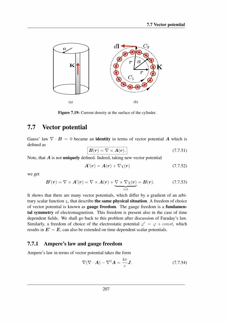
7.6.2 Example 2

As the second example we shall consider a magnetic field of superficial current densityK = Ke

3

localized at the surface of infinitely long cylinder with radius a. The am-plitude of the current density is equal to K = I

2⇡ a. A volume density of the current is

given by

J = Ke3

�(r � a), (7.6.49)

where r stands for the radial coordinate. A distribution of the current has cylindricalsymmetry. It suggest that magnetic field B should be restricted to the form (7.6.47). Letus consider intensity of electric current I(r) obtained by integration of current density(7.6.49) over disc with radius a and center at axis x3:

I(r) =

ZS(0,r)

da · J =

Z2⇡

0

d�

Z r

0

dr0r0 K�(r0 � a) = 2⇡ aK✓(r � a).

Plugging this expression to Ampere’s law we get

B(r) =4⇡

c

K a

r✓(r � a)�. (7.6.50)

A magnetic field vanish inside the cylinder and for r > a it is equivalent to the field ofa single wire placed at axis x3.

206

7.7 Vector potential

(a) (b)

Figure 7.19: Current density at the surface of the cylinder.

7.7 Vector potentialGauss’ law r · B = 0 became an identity in terms of vector potential A which isdefined as

B(r) = r⇥A(r). (7.7.51)

Note, that A is not uniquely defined. Indeed, taking new vector potential

A0(r) = A(r) +r�(r) (7.7.52)

we get

B0(r) = r⇥A0(r) = r⇥A(r) +r⇥r�(r)| {z }⌘ 0

= B(r). (7.7.53)

It shows that there are many vector potentials, which differ by a gradient of an arbi-trary scalar function �, that describe the same physical situation. A freedom of choiceof vector potential is known as gauge freedom. The gauge freedom is a fundamen-tal symmetry of electromagnetism. This freedom is present also in the case of timedependent fields. We shall go back to this problem after discussion of Faraday’s law.Similarly, a freedom of choice of the electrostatic potential '0 = ' + const, whichresults in E0 = E, can also be extended on time dependent scalar potentials.

7.7.1 Ampere’s law and gauge freedomAmpere’s law in terms of vector potential takes the form

r(r ·A)�r2A =4⇡

cJ . (7.7.54)

207


The gauge freedom can be used to eliminate the term r(r · A). Let us imagine thatwe have description of the physical system in terms of the vector potential A, wherer ·A 6= 0. We choose another vector potential A0 that satisfies condition r ·A0 = 0.Vanishing of divergence of A0 leads to differential equation on �

r ·A0 = 0 ) r2�(r) = �r ·A(r), (7.7.55)

which has solution in the form

�(r) = �ZRn

dnx0Dn(r � r0)r0 ·A(r0),

where r0 ·A(r0) is an explicitly given function. The potential A0 reads

A0(r) = A(r)�ZRn

dnx0rDn(r � r0)r0 ·A(r0). (7.7.56)

One can check that

r ·A0(r) = r ·A(r)�ZRn

dnx0 r2Dn(r � r0)| {z }�n(r�r

0)

r0 ·A(r0) = 0. (7.7.57)

It follows that equation (7.7.54) in terms of A0 is given by r2A0 = �4⇡cJ . In generality,

we shall omit 0 considering from the very beginning that A has been already chosen inappropriate way i.e.

r2A = �4⇡

cJ . (7.7.58)

A condition of vanishing of the divergence of vector potential

r ·A = 0 (7.7.59)

is known as Coulomb gauge condition. Note, that (7.7.58) is consistent with a Coulombgauge fixing (7.7.59) because r · J = 0.

7.7.2 Integral form of vector potentialLet us consider localized stationary currents J in V i.e J(r) = 0 for points p(r) /2 V .Taking into account that D

3

(R) = � 1

4⇡Rwe get

A(r) =1

c

ZV

d3x0 J(r0)

|r � r0| . (7.7.60)

This expression has the same form as electrostatic potential

'(r) =

ZV

d3x0 ⇢(r0)

|r � r0| .

208


7.7.2.1 Example: vector potential of infinitely long wire

A current density of infinitely long straight conducting wire is given by expression

J = I�(x0)�(y0)z.

It follows that the vector potential is given by integral

A(r) = zI

c

Z 1

�1

dz0

|r � z0z| . (7.7.61)

It is convenient to express (7.7.61) in cylindrical coordinates (⇢,�, z), what gives

A(r) = zI

c

Z 1

�1

dz0p⇢2 + (z � z0)2|

. (7.7.62)

In terms of new variable w := z0�z⇢

one gets

A(r) = zI

c

Z 1

�1

dwp1 + w2

= zI

carsinh(w)|1�1 ! 1. (7.7.63)

One has to face the problem of divergence of vector potential. On the other hand,magnetic field of infinitely long and straight conducting wire is given by B = 2I

c ⇢�, so

there must exist A(r) such that B = r⇥A. This problem can be solved as follows. Wechoose a cut-off for the integral and show that physics of the problem does not dependon the value of the cut-off. The cut-off is given by L such that

�L (z0 � z) L. (7.7.64)

It follows that vector potential takes the form

A(r) = zI

c

Z L

⇢

�L

⇢

dwp1 + w2

= 2zI

carsinh(w)|L/⇢

0

= 2zI

cln

24L

⇢+

s1 +

✓L

⇢

◆2

35 . (7.7.65)

In the limit L/⇢� 1 expression (7.7.65) can be approximated by the following one

A(r) = 2zI

cln

2L

⇢= 2z

I

c

ln⇢0

⇢+ ln

2L

⇢0

�, (7.7.66)

209


where ⇢0

is an arbitrary constant with dimension of length. It means, that the vectorpotential can be split into two parts: the part independent on the cut-off and the partwhich is constant and singular for L ! 1

A(r) = �z2I

cln

⇢

⇢0

+ z2I

cln

2L

⇢0| {z }

const

. (7.7.67)

Note, that presence of singular term has no effect on the form of magnetic field

B = r⇥A =2I

c

�

⇢. (7.7.68)

This is perhaps the simplest example which illustrate the idea that some singularquantities can be regularized through the cut-off procedure without affecting thephysical result. In quantum field theory there are many singular expressions which canbe regularized by appropriately chosen cut-off.

7.7.3 Magnetic fluxA magnetic flux through an oriented surface S is defined as

� =

ZS

B · da. (7.7.69)

Let S be an open surface with border C = @S. Orientation of the curve C must beconsistent with orientation of S. Making use of Stokes theorem we get

� =

ZS

(r⇥A) · da =

IC

A · dl. (7.7.70)

Note, that the gauge freedom has no effect on value of magnetic flux because r� · dl =d� so

HCd� = 0.

7.7.3.1 Example: vector potential of infinitely long solenoid

Relation between magnetic flux and the line integral involving vector potential can beused to determine the vector potential. As example we shall consider an infinitely longsolenoid with radius a and n turns per unit of length. A current with intensity I flows ina wire of the solenoid. When number of turns per unit of length n is sufficiently high,than the current in the solenoid wire can be substituted by a surface current densityK = nI

J = nI�(r � a)�.

210


Magnetic field in region r > a should be zero in such a case. Applying Ampere’s lawfor small oriented rectangle perpendicular to surface of the solenoid and plugging theansatz B(r) = Bz we get B�l = 4⇡

cnI�l. The magnetic field reads

B =4⇡

cnI✓(a� r)z. (7.7.71)

We assume the following ansatz

A(r) = A(r)�. (7.7.72)

Note, that proportionality to vector � is easy to be guess since r2A = �4⇡cJ where J

is proportional to �. Let C be a circle in the plane xy with center at axis z and radius r.The indentity I

C

A · dl =ZS

B · da, (7.7.73)

where dl = � rd� and da = zrdrd� readsZ2⇡

0

A(r)rd� =

Z2⇡

0

d�

Z r

0

dr0r04⇡

cnI✓(a� r0),

whereR r

0

dr0r0✓(a� r0) = r2

2

for r < a andR r

0

dr0r0✓(a� r0) = a2

2

for r > a. It gives

2⇡rA(r) =(2⇡)2

cnI

⇥r2✓(a� r) + a2✓(r � a)

⇤and finally

A(r) =2⇡nI

c

r✓(a� r) +

a2

r✓(r � a)

��. (7.7.74)

This result shows that vector potential is not zero outside of the solenoid r > a, however,in this it is irrotational A / 1

r�.

7.7.4 Magnetic field of a distant loopIn this section we compute vector potential and magnetic field of a loop with currentintensity I . We shall solve this problem in region distant from the loop |r0| ⌧ |r|, seeFIg.7.20. The potential is given by integral

A(r) =I

c

IC

dr0

|r � r0| . (7.7.75)

211


Figure 7.20: Loop with current I .

Expanding expression |r � r0|�1 we get

|r � r0|�1 =1

r

✓1� 2

r · r0

r2+

r02

r2

◆�1/2

=1

r+

r · r0

r3+ . . .

The vector potential has the following leading terms

A(r) =I

c r

IC

dr0 +I

c r3

IC

(r · r0)dr0 + . . . (7.7.76)

whereHCdr0 = 0. It means, that there is no contribution from the monopole term. A

second integral can be written in slightly different form. Considering sum of identities

(r · r0)dr0 = d[(r · r0)r0]� (r · dr0)r0

(r · r0)dr0 = (r0 ⇥ dr0)⇥ r + (r · dr0)r0

we find that(r · r0)dr0 =

1

2(r0 ⇥ dr0)⇥ r +

1

2d[(r · r0)r0], (7.7.77)

where term with total derivative does not contribute to the integral. The leading term ofthe vector potential reads

A(r) =

✓I

2c

IC

(r0 ⇥ dr0)

◆| {z }

m

⇥ r

r3+ . . .

where m is magnetic moment of the loop. A leading term for vector potential is of theform

A(r) = m⇥ r

r3(7.7.78)

212


This expression can be also interpreted as a vector potential of magnetic point-likedipole at r = 0. There is a formal analogy between this formula and expression forelectrostatic potential: '(r) = p · r

r3.

Magnetic field of the loop has the form

B = r⇥A = �r⇥✓m⇥r1

r

◆= r

(m ·r)

1

r

��mr2

1

r. (7.7.79)

For solution in a region far from the center the vector r never takes zero value. Thenfunction r�1 is harmonic one: r2r�1 = 0. The magnetic field reads

B(r) = eimj@i@j

1

r= eim

j 3xixj � r2�ij

r5

what can be cast in the form

B(r) =3(m · r)r � r2m

r5. (7.7.80)

A magnetic field of a point-like magnetic dipole with magnetic moment m has the

(a) (b)

Figure 7.21: (a) Finite size electric dipole. (b) Finite size magnetic dipole (a loop withelectric current).

same form as electric field of point-like electric dipole with electric dipole moment p

E(r) =3(p · r)r � r2p

r5. (7.7.81)

213


Such electric fields can be written as E = �r'(r). It follows, that it must exist a scalarfunction (r) such that

B(r) = �r (r). (7.7.82)

Function (r) is called magnetic potential. Such a function can be determinedonly in regions where r ⇥ B(r) = 0. In current example, this condition is satisfiedin whole space except the point r = 0. It explains why we were managed to representa magnetic field as a gradient of scalar potential. A vector potential is more adequatebecause it solves equation r · B = 0 in regions where there are currents and outsidethese region.

Magnetic field of a finite loop and finite-size electric field of finite size electric dipoleare similar only in region far from their sources and they differ significantly in regionclose the sources.

214

Documents

7 Magnetic ﬁeld of stationary currents - UFSCklimas.paginas.ufsc.br/files/2017/10/chapter7.pdf · electricity, galvanism and magnetism at the university in Copenhagen. ... cathode