Embed Size (px)
Citation preview

600.325/425 Declarative Methods - J. Eisner
1
A few methods for learning binary classifiers

600.325/425 Declarative Methods - J. Eisner
2
Fundamental Problem of Machine Learning: It is ill-posed
slide thanks to Tom Dietterich (modified)

600.325/425 Declarative Methods - J. Eisner
3
Learning Appears Impossible
There are 216 = 65536 possible boolean functions over four input features.
Why? Such a function is defined by 24 = 16 rows. So its output column has 16 slots for answers. There are 216 ways it could fill those in.
slide thanks to Tom Dietterich (modified)
x x x x y ? ? ? ? ? ? ? ? ? ? ? ? ? ? ? ?
spam detection

600.325/425 Declarative Methods - J. Eisner
4
Learning Appears Impossible
There are 216 = 65536 possible boolean functions over four input features.
Why? Such a function is defined by 24 = 16 rows. So its output column has 16 slots for answers. There are 216 ways it could fill those in.
We can’t figure out which one is correct until we’ve seen every possible input-output pair.
After 7 examples, we still have 9 slots to fill in, or 29 possibilities.
slide thanks to Tom Dietterich (modified)
x1 x2 x3 x4 y ? ? ? ? ? ? ? ? ?
spam detection

600.325/425 Declarative Methods - J. Eisner
5
Solution: Work with a restricted hypothesis space
We need to generalize from our few training examples!
Either by applying prior knowledge or by guessing, we choose a space of hypotheses H that is smaller than the space of all possible Boolean functions: simple conjunctive rules m-of-n rules linear functions multivariate Gaussian joint probability distributions etc.
slide thanks to Tom Dietterich (modified)

600.325/425 Declarative Methods - J. Eisner
6
Illustration: Simple Conjunctive Rules There are only 16
simple conjunctions (no negation)
Try them all! But no simple rule
explains our 7 training examples.
The same is true for simple disjunctions.
slide thanks to Tom Dietterich (modified)

600.325/425 Declarative Methods - J. Eisner
7
A larger hypothesis space:m-of-n rules
At least m of n specified variables must be true
There are 32 possible rules
Only one rule is consistent!
slide thanks to Tom Dietterich (modified)

600.325/425 Declarative Methods - J. Eisner
8
Two Views of Learning View 1: Learning is the removal of our remaining uncertainty about
the truth Suppose we knew that the unknown function was an m-of-n boolean function.
Then we could use the training examples to deduce which function it is. View 2: Learning is just an engineering guess – the truth is too
messy to try to find Need to pick a hypothesis class that is
big enough to fit the training data “well,” but not so big that we overfit the data & predict test data poorly.
Can start with a very small class and enlarge it until it contains an hypothesis that fits the training data perfectly.
Or we could stop enlarging sooner, when there are still some errors on training data. (There’s a “structural risk minimization” formula for knowing when to stop! - a loose bound on the test data error rate.)
slide thanks to Tom Dietterich (modified)

600.325/425 Declarative Methods - J. Eisner
9
Balancing generalization and overfitting
figures from a paper by Mueller et al.
which boundary?go for simplicity
or accuracy?
more training data makes the choice more obvious
?

600.325/425 Declarative Methods - J. Eisner
10
We could be wrong!
1. Multiple hypotheses in the class might fit the data
2. Our guess of the hypothesis class could be wrong Within our class, the only answer was
“y=true [spam] iff at least 2 of {x1,x3,x4} say so” But who says the right answer is an m-of-n rule at all? Other hypotheses outside the class also work:
y=true iff … (x1 xor x3) ^ x4 y=true iff … x4 ^ ~x2
example thanks to Tom Dietterich

600.325/425 Declarative Methods - J. Eisner
11
Two Strategies for Machine Learning Use a “little language” to define a hypothesis class H that’s tailored
to your problem’s structure (likely to contain a winner) Then use a learning algorithm for that little language Rule grammars; stochastic models (HMMs, PCFGs …); graphical
models (Bayesian nets, Markov random fields …) Dominant view in 600.465 Natural Language Processing Note: Algorithms for graphical models are closely related to
algorithms for constraint programming! So you’re on your way.
Just pick a flexible, generic hypothesis class H Use a standard learning algorithm for that hypothesis class Decision trees; neural networks; nearest neighbor; SVMs What we’ll focus on this week It’s now crucial how you encode your problem as a feature vector
parts of slide thanks to Tom Dietterich

600.325/425 Declarative Methods - J. Eisner
12
Memory-Based Learning
E.g., k-Nearest Neighbor
Also known as “case-based” or “example-based” learning

600.325/425 Declarative Methods - J. Eisner
13
Intuition behind memory-based learning Similar inputs map to similar outputs
If not true learning is impossible If true learning reduces to defining “similar”
Not all similarities created equal guess J. D. Salinger’s weight
who are the similar people? similar occupation, age, diet, genes, climate, …
guess J. D. Salinger’s IQ similar occupation, writing style, fame, SAT score, …
Superficial vs. deep similarities? B. F. Skinner and the behaviorism movement
parts of slide thanks to Rich Caruana
what do brains actually do?

600.325/425 Declarative Methods - J. Eisner
14
1-Nearest Neighbor Define a distance d(x1,x2) between any 2 examples
examples are feature vectors so could just use Euclidean distance …
Training: Index the training examples for fast lookup. Test: Given a new x, find the closest x1 from training.
Classify x the same as x1 (positive or negative)
Can learn complex decision boundaries As training size , error rate is at most 2x the Bayes-optimal rate (i.e., the error rate you’d get from knowing the true model that generated the data – whatever it is!)
parts of slide thanks to Rich Caruana
600.325/425 Declarative Methods - J. Eisner
15From Hastie, Tibshirani, Friedman 2001 p418
slide thanks to Rich Caruana (modified)
1-Nearest Neighbor – decision boundary

600.325/425 Declarative Methods - J. Eisner
16
k-Nearest Neighbor
Average of k points more reliable when: noise in training vectors x noise in training labels y classes partially overlap
attribute_1
attr
ibut
e_2
++
+
+
+
++++
o
o
ooo
ooo oo
o
+
++o
o o
slide thanks to Rich Caruana (modified)
Instead of picking just the single nearest neighbor, pick the k nearest neighbors and have them vote

600.325/425 Declarative Methods - J. Eisner
17From Hastie, Tibshirani, Friedman 2001 p418
slide thanks to Rich Caruana (modified)
1 Nearest Neighbor – decision boundary

600.325/425 Declarative Methods - J. Eisner
18From Hastie, Tibshirani, Friedman 2001 p418
slide thanks to Rich Caruana (modified)
15 Nearest Neighbors – it’s smoother!

600.325/425 Declarative Methods - J. Eisner
19
How to choose “k”
Odd k (often 1, 3, or 5): Avoids problem of breaking ties (in a binary classifier)
Large k: less sensitive to noise (particularly class noise) better probability estimates for discrete classes larger training sets allow larger values of k
Small k: captures fine structure of problem space better may be necessary with small training sets
Balance between large and small k What does this remind you of?
As training set approaches infinity, and k grows large, kNN becomes Bayes optimal
slide thanks to Rich Caruana (modified)

600.325/425 Declarative Methods - J. Eisner
20
From Hastie, Tibshirani, Friedman 2001 p419
slide thanks to Rich Caruana (modified)
why?

600.325/425 Declarative Methods - J. Eisner
21
Cross-Validation
Models usually perform better on training data than on future test cases
1-NN is 100% accurate on training data! “Leave-one-out” cross validation:
“remove” each case one-at-a-time use as test case with remaining cases as train set average performance over all test cases
LOOCV is impractical with most learning methods, but extremely efficient with MBL!
slide thanks to Rich Caruana

600.325/425 Declarative Methods - J. Eisner
22
Distance-Weighted kNN hard to pick large vs. small k
may not even want k to be constant use large k, but more emphasis on nearer neighbors?
),(exp
1often or
),(
1 maybeor
),(
1
:NN-k for the weightsrelative define We
labels their , and NN-k theare , e wher
)(
11
1
1
xxDistxxDistxxDistw
yyxx
w
ywxprediction
iiii
kk
k
ii
k
iii
parts of slide thanks to Rich Caruana

600.325/425 Declarative Methods - J. Eisner
23
Combining k-NN with other methods, #1 Instead of having the k-NN simply vote, put
them into a little machine learner! To classify x, train a “local” classifier on its k
nearest neighbors (maybe weighted). polynomial, neural network, …
parts of slide thanks to Rich Caruana

600.325/425 Declarative Methods - J. Eisner
24
Now back to that distance function
Euclidean distance treats all of the input dimensions as equally important
attribute_1
attr
ibut
e_2
++
+
+
+
++++
oo
ooo
ooo oo
o
parts of slide thanks to Rich Caruana

600.325/425 Declarative Methods - J. Eisner
25
These o’s are now “closer” to + than to each other
Now back to that distance function
Euclidean distance treats all of the input dimensions as equally important
Problem #1: What if the input represents physical weight not in pounds but
in milligrams? Then small differences in physical weight dimension have a huge
effect on distances, overwhelming other features. Should really correct for these arbitrary “scaling” issues.
One simple idea: rescale weights so that standard deviation = 1.
+o o
+
weight (lb)
attr
ibut
e_2
++
+
++ +
+o
o
oo oo
ooo
weight (mg)
attr
ibut
e_2
+
++
+
++ +
++
oo
oo
o
oo
ooo
obad

600.325/425 Declarative Methods - J. Eisner
26
Now back to that distance function
Euclidean distance treats all of the input dimensions as equally important
Problem #2: What if some dimensions more correlated with true label?
(more relevant, or less noisy) Stretch those dimensions out so that they are more
important in determining distance. One common technique is called “information gain.”
parts of slide thanks to Rich Caruana
most relevant attribute
attr
ibut
e_2
++
+
+
+
+++
++ o o
o
oo
o
o
o
oo
o
attr
ibut
e_2
most relevant attribute
++
+
+
+
+++
++ o o
o
oo
o
o
o
oo
o
good

600.325/425 Declarative Methods - J. Eisner
27
Weighted Euclidean Distance
large weight si attribute i is more important
small weight si attribute i is less important
zero weight si attribute i doesn’t matter
N
iiii xxsxxd
1
2')',(
slide thanks to Rich Caruana (modified)

600.325/425 Declarative Methods - J. Eisner
28
Now back to that distance function
Euclidean distance treats all of the input dimensions as equally important
Problem #3: Do we really want to decide separately and theoretically how to
scale each dimension? Could simply pick dimension scaling factors to maximize
performance on development data. (maybe do leave-one-out) Similarly, pick number of neighbors k and how to weight them.
Especially useful if performance measurement is complicated(e.g., 3 classes and differing misclassification costs).
attribute_1
attr
ibut
e_2
++
+
+
+
+ +++
o
o
o oo
oooo
o
o

600.325/425 Declarative Methods - J. Eisner
29
should replot on log scale before measuring dist
Now back to that distance function
Euclidean distance treats all of the input dimensions as equally important
Problem #4: Is it the original input dimensions that we want to scale? What if the true clusters run diagonally? Or curve? We can transform the data first by extracting a different,
useful set of features from it: Linear discriminant analysis Hidden layer of a neural network
attribute_1
attr
ibut
e_2
+
++
+
+
+
+
+
+
+o
o
o
oo
o
o
o
oo
o
want to stretch
along this dimension exp(attribute_1)
attr
ibut
e_2
++
+
+
+
+++
++ o o
o
o
o
o
o
o
o
o
i.e., redescribe the data by how a different type of learned classifier internally sees it
600.325/425 Declarative Methods - J. Eisner
30
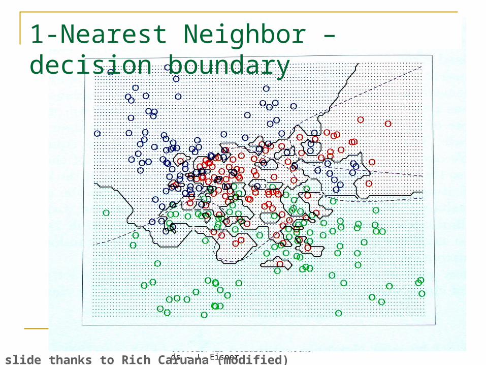
Now back to that distance function
Euclidean distance treats all of the input dimensions as equally important
Problem #5: Do we really want to transform the data globally? What if different regions of the data space behave differently? Could find 300 “nearest” neighbors (using global transform), then
locally transform that subset of the data to redefine “near” Maybe could use decision trees to split up the data space first
attribute_1at
trib
ute_
2+
++
+
++
+ ++
+ oo o
o
oo
o
o
o
oo
o
o++ ++ ++
+
++
ooo
o
oo oo oo o
?
?

600.325/425 Declarative Methods - J. Eisner
31
Why are we doing all this preprocessing? Shouldn’t the user figure out a smart way to transform the
data before giving it to k-NN?
Sure, that’s always good, but what will the user try? Probably a lot of the same things we’re discussing. She’ll stare at the training data and try to figure out how to
transform it so that close neighbors tend to have the same label. To be nice to her, we’re trying to automate the most common
parts of that process – like scaling the dimensions appropriately. We may still miss patterns that her visual system or expertise can
find. So she may still want to transform the data. On the other hand, we may find patterns that would be hard for
her to see.

600.325/425 Declarative Methods - J. Eisner
32
split on feature that reduces
our uncertainty most
1607/1704 = 0.943 694/5977 = 0.116
Tangent: Decision Trees(a different simple method)
example thanks to Manning & Schütze
Is this Reuters article an Earnings Announcement?
2301/7681 = 0.3 of all docs
contains “cents” < 2 times contains “cents” 2 times
contains “versus” < 2 times
contains “versus”
2 times
contains “net”
< 1 time
contains “net”
1 time
1398/1403 = 0.996
209/301 = 0.694
“yes”
422/541 = 0.780
272/5436 = 0.050
“no”

600.325/425 Declarative Methods - J. Eisner
33
Booleans, Nominals, Ordinals, and Reals Consider attribute value differences:
(xi – x’i): what does subtraction do?
Reals: easy! full continuum of differences Integers: not bad: discrete set of differences Ordinals: not bad: discrete set of differences Booleans: awkward: hamming distances 0 or 1 Nominals?not good! recode as Booleans?
slide thanks to Rich Caruana (modified)

600.325/425 Declarative Methods - J. Eisner
34
“Curse of Dimensionality”” Pictures on previous slides showed 2-dimensional data What happens with lots of dimensions? 10 training samples cover the space less & less well …
images thanks to Charles Annis
600.325/425 Declarative Methods - J. Eisner
35
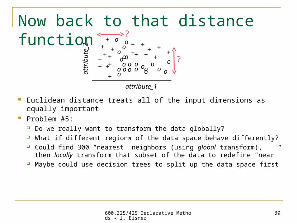
“Curse of Dimensionality””
A deeper perspective on this: Random points chosen in a high-dimensional space tend to all be
pretty much equidistant from one another! (Proof: in 1000 dimensions, the squared distance between two random
points is a sample variance of 1000 coordinate distances. Since 1000 is large, this sample variance is usually close to the true variance.)
So each test example is about equally close to most training examples.
We need a lot of training examples to expect one that is unusually close to the test example.
images thanks to Charles Annis
Pictures on previous slides showed 2-dimensional data What happens with lots of dimensions? 10 training samples cover the space less & less well …

600.325/425 Declarative Methods - J. Eisner
36
“Curse of Dimensionality”” also, with lots of dimensions/attributes/features, the
irrelevant ones may overwhelm the relevant ones:
So the ideas from previous slides grow in importance: feature weights (scaling)
feature selection (try to identify & discard irrelevant features) but with lots of features, some irrelevant ones will probably
accidentally look relevant on the training data smooth by allowing more neighbors to vote (e.g., larger k)
relevant
i
irrelevant
jjjii xxxxxxd
1 1
22 '')',(
slide thanks to Rich Caruana (modified)
600.325/425 Declarative Methods - J. Eisner
37
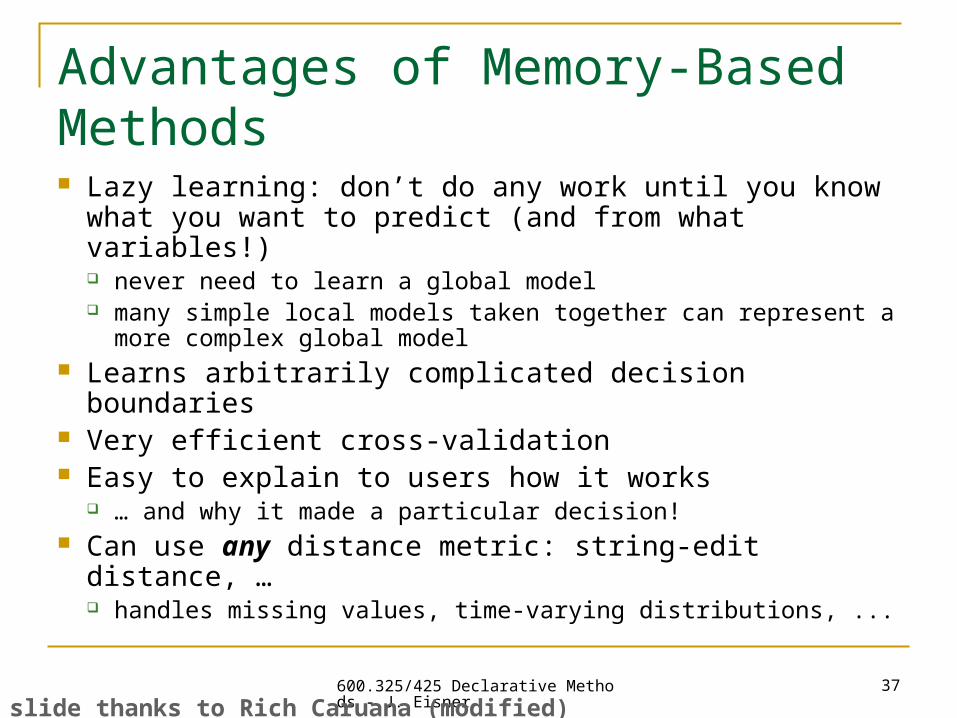
Advantages of Memory-Based Methods Lazy learning: don’t do any work until you know
what you want to predict (and from what variables!) never need to learn a global model many simple local models taken together can represent a
more complex global model Learns arbitrarily complicated decision boundaries Very efficient cross-validation Easy to explain to users how it works
… and why it made a particular decision! Can use any distance metric: string-edit distance, …
handles missing values, time-varying distributions, ...
slide thanks to Rich Caruana (modified)

600.325/425 Declarative Methods - J. Eisner
38
Weaknesses of Memory-Based Methods Curse of Dimensionality
often works best with 25 or fewer dimensions Classification runtime scales with training set size
clever indexing may help (K-D trees? locality-sensitive hash?) large training sets will not fit in memory
Sometimes you wish NN stood for “neural net” instead of “nearest neighbor” Simply averaging nearby training points isn’t very subtle Naive distance functions are overly respectful of the input encoding
For regression (predict a number rather than a class), the extrapolated surface has discontinuities
slide thanks to Rich Caruana (modified)

600.325/425 Declarative Methods - J. Eisner
39
Current Research in MBL
Condensed representations to reduce memory requirements and speed-up neighbor finding to scale to 106–1012 cases
Learn better distance metrics Feature selection Overfitting, VC-dimension, ... MBL in higher dimensions MBL in non-numeric domains:
Case-Based or Example-Based Reasoning Reasoning by Analogy
slide thanks to Rich Caruana

600.325/425 Declarative Methods - J. Eisner
40
References
Locally Weighted Learning by Atkeson, Moore, Schaal
Tuning Locally Weighted Learning by Schaal, Atkeson, Moore
slide thanks to Rich Caruana

600.325/425 Declarative Methods - J. Eisner
41
Closing Thought
In many supervised learning problems, all the information you ever have about the problem is in the training set.
Why do most learning methods discard the training data after doing learning?
Do neural nets, decision trees, and Bayes nets capture all the information in the training set when they are trained?
Need more methods that combine MBL with these other learning methods. to improve accuracy for better explanation for increased flexibility
slide thanks to Rich Caruana

600.325/425 Declarative Methods - J. Eisner
42
Linear Classifiers

600.325/425 Declarative Methods - J. Eisner
43
Linear regression – standard statistics
As usual, input is a vector x Output is a number y=f(x)
x1
x2x2
*
**
*
*
*
*
*
**
**
*
*
*
*
*
**
*
y

600.325/425 Declarative Methods - J. Eisner
44
Linear regression – standard statistics
As usual, input is a vector x Output is a number y=f(x) Linear regression:
bxwxwxw
bxw
bxwy
ii
i
332211
yx1
x2
*
**
*
**
*
*
*
**
**
*
*
*
*
*
**
*

600.325/425 Declarative Methods - J. Eisner
45
Linear classification
As usual, input is a vector x Output is a class y {-,+} Linear classification:
0 if
0 if
bxw- y
bxwy
yx1
x2
++
++
+
++
+
++
+ -
--
-
-
-
--
-
-
-
decision boundary(a straight line splitting the 2-D data space;in higher dimensions, a flatplane or hyperplane)
threshold bweight vector w(since classifier asks: does w.x exceed –b, crossing a threshold?b often called “bias term,” since adjusting it will bias the classifier toward picking + or -)

600.325/425 Declarative Methods - J. Eisner
46
'x
thiscall'w
thiscall
0),1()(b, as
0 Rewrite
xw
bxw
Simplify the notation: Eliminate b (just another reduction: problem may look easier without b, but isn’t)
0'' form theof classifier afor look then and
),,,1(' with ),,(
exampleeach replace s,other wordIn
2121
xw
xxxxxx
yx1
x2
++
++
+
++
+
++
+ -
--
-
-
-
--
-
-
- term)bias theis ' (so 0w

600.325/425 Declarative Methods - J. Eisner
47
Training a linear classifier
Given some supervised training data (usually high-dimensional) What is the best linear classifier (defined by weight vector w’)? Surprisingly, lots of algorithms! Three cases to think about:
1. The training data are linearly separable ( a hyperplane that perfectly divides + from -;then there are probably many such hyperplanes; how to pick?)
2. The training data are almost linearly separable(but a few noisy or unusual training points get in the way; we’ll just allow some error on the training set)
3. The training data are linearly inseparable(the right decision boundary doesn’t look like a hyperplane at all;we’ll have to do something smarter)

600.325/425 Declarative Methods - J. Eisner
48
Linear separability
images thanks to Tom Dietterich
linearly separable
?

600.325/425 Declarative Methods - J. Eisner
49
Linear separability
images thanks to Tom Dietterich
almost linearly separable
?
linearly inseparableIn fact, the simplest case:y = x1 xor x2
???
01
Can learn e.g. concepts in the “at least m-of-n” family (what are w and b in this case?)
But can’t learn arbitrary boolean concepts like xor

600.325/425 Declarative Methods - J. Eisner
50
?
Finding a separating hyperplane If the data really are separable, can set this up
as a linear constraint problem with real values: Training data: (x1, +), (x2, +), (x3, -), … Constraints: wx1 $> 0, wx2 $> 0, wx3 $< 0,
… Variables: the numeric components of vector w But infinitely many solutions for solver to find … … luckily, the standard linear
programming problem gives a declarative way to say which solution we want: minimize some cost subject to the constraints.
So what should the cost be?

600.325/425 Declarative Methods - J. Eisner
51
?
Finding a separating hyperplane Advice: stay in the middle of your lane;
drive in the center of the space available to you
hyperplane shouldn’t veer too close to any of the training points.

600.325/425 Declarative Methods - J. Eisner
52
Finding a separating hyperplane Advice: stay in the middle of your lane;
drive in the center of the space available to you Define cost of a separating hyperplane =
the distance to the nearest training point.
hyperplane shouldn’t veer too close to any of the training points.
maximize this“margin”

600.325/425 Declarative Methods - J. Eisner
53
Advice: stay in the middle of your lane;drive in the center of the space available to you
Define cost of a separating hyperplane = the distance to the nearest training point.
In the 2-dimensional case, usually at most 3 points can be nearest: hyperplane drives right between them. The nearest training points to the hyperplane are called the
“support vectors” (more in more dims), and are enough to define it.
Finding a separating hyperplane
hyperplane shouldn’t veer too close to any of the training points.
maximize this“margin”
?

600.325/425 Declarative Methods - J. Eisner
54
Advice: stay in the middle of your lane;drive in the center of the space available to you
Define cost of a separating hyperplane = the distance to the nearest training point.
In the 2-dimensional case, usually at most 3 points can be nearest: hyperplane drives right between them. The nearest training points to the hyperplane are called the
“support vectors” (more in more dims), and are enough to define it.
Finding a separating hyperplane
hyperplane shouldn’t veer too close to any of the training points.
maximize this“margin”

600.325/425 Declarative Methods - J. Eisner
55
Finding a separating hyperplane http://www.site.uottawa.ca/~gcaron/LinearApplet/LinearApplet.htm
Question: If you believe in nearest neighbors, why would the idea of maximizing the margin also be attractive?
Compare SVMs and nearest neighbor for test points that are near a training point.
Compare SVMs and nearest neighbor for test points that are far from a training point.

600.325/425 Declarative Methods - J. Eisner
56
Advice: stay in the middle of your lane;drive in the center of the space available to you
Define cost of a separating hyperplane = the distance to the nearest training point.
How do we define this cost in our constraint program?? Cost $= min([distance to point 1, distance to point 2, …])
Big nasty distance formulas. Instead we’ll use a trick that lets us use a specialized solver.
Finding a separating hyperplane
hyperplane shouldn’t veer too close to any of the training points.
maximize this“margin”

600.325/425 Declarative Methods - J. Eisner
57
Finding a separating hyperplane: trick To get a positive example x on the
correct side of the red line, pick w so that wx > 0.
To give it an extra margin, try to get wx to be as big as possible!
Good: wx is bigger for points farther from red boundary (it is the height of the gray surface).
Oops! It’s easier to double wx simply by doubling w. That only changes the slope of
the gray plane. It doesn’t change the red line
where wx = 0. So same margin.
yx1
x2
++
++
+
++
+
++
+ -
--
-
-
-
--
-
-
-
or for negative examples, wx < 0 and as negative as possible
600.325/425 Declarative Methods - J. Eisner
58
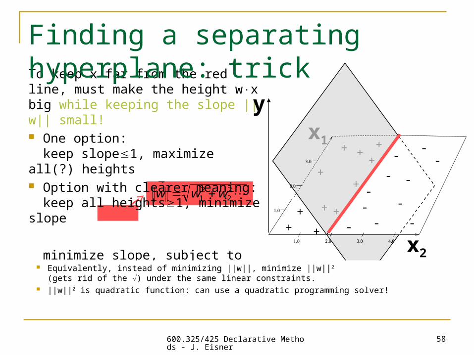
2
221 www
To keep x far from the red line, must make the height wx big while keeping the slope ||w|| small! One option:
keep slope1, maximize all(?) heights Option with clearer meaning:
keep all heights1, minimize slope
minimize slope, subject to wx 1 for each (x,+)wx -1 for each (x,-)
Finding a separating hyperplane: trick
yx1
x2
++
++
+
++
+
++
+ -
--
-
-
-
--
-
-
-
Equivalently, instead of minimizing ||w||, minimize ||w||2 (gets rid of the ) under the same linear constraints.
||w||2 is quadratic function: can use a quadratic programming solver!

600.325/425 Declarative Methods - J. Eisner
59
Support Vector Machines (SVMs) That’s what you just saw!
SVM = linear classifier that’s chosen to maximize the “margin.” Margin = distance from the hyperplane decision boundary to its
closest training points (the “support vectors”).
To choose the SVM, use a quadratic programming solver. Finds the best solution in polynomial time. Mixes soft and hard constraints:
Minimize ||w||2 while satisfying some wx 1 and wx -1 constraints. That is, find a maximum-margin separating hyperplane.
But what if the data aren’t linearly separable? Constraint program will have no solution …

600.325/425 Declarative Methods - J. Eisner
60
Let’s stay declarative: edit the constraint program to allow but penalize misclassification.
Instead of requiring wx 1, only require wx + fudge_factor 1 One fudge factor (“slack variable”) for each example
Easy to satisfy constraints now! Major fudging everywhere! Better keep the fudge factors small: just add them to the cost ||w||2
It’s not free to “move individual points” to improve separability
SVMs that tolerate noise(if the training data aren’t quite linearly separable)
New total cost function is a sum trying to balance two objectives:
BenefitsGetting an extra inch of margin: $100
(done by reducing ||w||2 by some amount while keeping wx+fudge
1)
CostsMoving one point by one inch: $3(done by fudging the plane height
wx as if the point had been moved)
Development data to pick these relative numbers: Priceless
600.325/425 Declarative Methods - J. Eisner
61
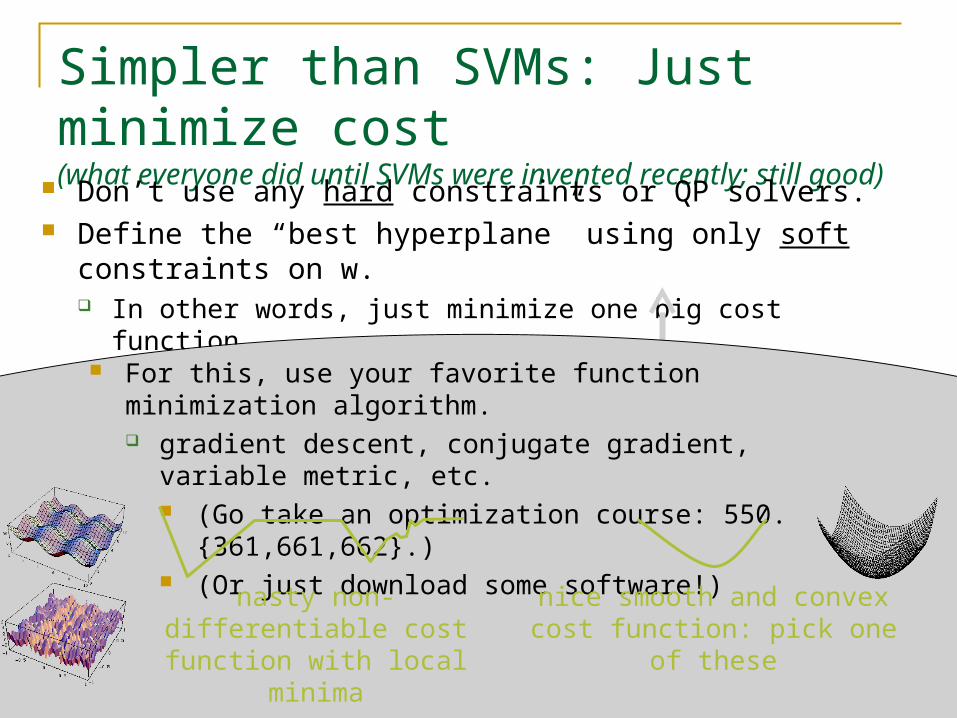
Simpler than SVMs: Just minimize cost(what everyone did until SVMs were invented recently; still good)
Don’t use any hard constraints or QP solvers. Define the “best hyperplane” using only soft constraints on w.
In other words, just minimize one big cost function.
What should the cost function be?
For this, use your favorite function minimization algorithm. gradient descent, conjugate gradient, variable metric,
etc. (Go take an optimization course: 550.
{361,661,662}.) (Or just download some software!)nasty non-differentiable cost function with local
minima
nice smooth and convex cost function: pick one of
these

600.325/425 Declarative Methods - J. Eisner
62
Simpler than SVMs: Just minimize cost What should the cost function be?
Training data: (x1, +), (x2, +), (x3, -), … Try to ensure that wx 1 for the positive examples,
wx -1 for the negative examples. Impose some kind of cost for bad approximations “”. Every example contributes to the total cost.
(Whereas SVM cost only cares about closest examples.)
We’re not saying “wx as big as possible” …Want wx to be positive, not merely “big.” The difference between -1 and 1 is “special” (it crosses the 0 threshold)
… not like the difference between -3 and -1 or 7 and 9.Anyway, one could make wx bigger just by doubling w (as with SVMs).So wx 2 shouldn’t be twice as good as wx 1. (Some methods even say it’s worse!)

600.325/425 Declarative Methods - J. Eisner
63
Simpler than SVMs: Just minimize cost What should the cost function be?
Training data: (x1, +), (x2, +), (x3, -), … Try to ensure that wx 1 for the positive examples,
wx -1 for the negative examples. Impose some kind of cost for bad approximations “”. Every example contributes to the total cost.
(Whereas SVM cost only cares about closest examples.)
The cost that classifier w incurs on a particular example is called its “loss” on that example.
Just define it, then look for a classifier that minimizes the total loss over all examples.

600.325/425 Declarative Methods - J. Eisner
64
Some loss functions …
-3 -2 -1 0 1 2 3 4
w.x
loss
(i
f x
is a
po
siti
ve e
xam
ple
) squared error
0-1 loss
perceptron
logistic

600.325/425 Declarative Methods - J. Eisner
65
“Least Mean Squared Error” (LMS)
-3 -2 -1 0 1 2 3 4
w.x
loss
(i
f x
is a
po
siti
ve e
xam
ple
)Training data: (x1, +), (x2, +), (x3, -), … Cost = (wx1 – 1)2 + (wx2 – 1)2 + (wx3 – (-1))2 + …
We demand wx 1 for a pos. example x!Complain loudly if wx is quite negative Equally loudly if wx is quite positive (?!)

600.325/425 Declarative Methods - J. Eisner
66
“Least Mean Squared Error” (LMS)
-3 -2 -1 0 1 2 3 4
w.x
loss
(i
f x
is a
po
siti
ve e
xam
ple
)Training data: (x1, +), (x2, +), (x3, -), … Cost = (wx1 – 1)2 + (wx2 – 1)2 + (wx3 – (-1))2 + …
The function optimizer will try to adjust w to drive wx closer to 1.
Simulates a marble rolling downhill.

600.325/425 Declarative Methods - J. Eisner
67
“Least Mean Squared Error” (LMS)
-3 -2 -1 0 1 2 3 4
w.x
loss
(i
f x
is a
po
siti
ve e
xam
ple
)Training data: (x1, +), (x2, +), (x3, -), … Cost = (wx1 – 1)2 + (wx2 – 1)2 + (wx3 – (-1))2 + …
The function optimizer will try to adjust w to drive wx closer to 1.
Gradient descent rule for this loss function (repeat until convergence):
If wx is too small (< 1), increase w byx. If wx is too big (> 1), decrease w by x.
(Why does this work?) is a tiny number but is proportional
to how big or small wx was.

600.325/425 Declarative Methods - J. Eisner
68
-3 -2 -1 0 1 2 3 4
w.x
loss
(i
f x
is a
po
siti
ve e
xam
ple
)
squared error
0-1 loss
LMS versus 0-1 loss
Why might that cost be a better thing to minimize?Why isn’t it a perfect thing to minimize?
(compare with SVMs)Why would it be a difficult function to minimize?
To see why LMS loss is weird, compare it to 0-1 loss (blue line). What is the total 0-1 loss over all training examples?

600.325/425 Declarative Methods - J. Eisner
69
-3 -2 -1 0 1 2 3 4
w.x
loss
(i
f x
is a
po
siti
ve e
xam
ple
)
squared error
0-1 loss
perceptron
Perceptron algorithm (old!)
If wx < 0, increase w byx. (Almost the same as before!)
If wx > 0, w is working: leave it alone.Since yellow line is straight, is a constant – whereas for purple line (LMS), it was bigger when wx was more negative. (So purple
maybe tried too hard on hopeless examples.)
This yellow loss function is easier to minimize. Its gradient descent rule is the “perceptron algorithm”:

600.325/425 Declarative Methods - J. Eisner
70
-3 -2 -1 0 1 2 3 4
w.x
loss
(i
f x
is a
po
siti
ve e
xam
ple
) squared error
0-1 loss
perceptron
logistic
Logistic regression The light blue loss function gets back a “margin”-like idea:
log (exp(wx) / (1 + exp(wx)))
If x is misclassified, resembles perceptron
lossEven if x is correctly
classified, still prefer wx to exceed 0 by even
more…
Can’t reduce loss much more here. More benefit if we adjust w to help other examples.
… within reason

600.325/425 Declarative Methods - J. Eisner
71
-3 -2 -1 0 1 2 3 4
w.x
loss
(i
f x
is a
po
siti
ve e
xam
ple
)
The gradient descent rule is again similar. Again, only difference is how is computed.
Logistic regression The light blue loss function gets back a “margin”-like idea:
log (exp(wx) / (1 + exp(wx)))
600.325/425 Declarative Methods - J. Eisner
72
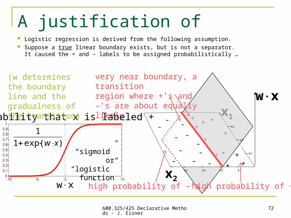
A justification of logistic regression Logistic regression is derived from the following assumption. Suppose a true linear boundary exists, but is not a separator.
It caused the + and – labels to be assigned probabilistically …
wxx1
x2
++
+ +
+
++
+
+ +
+-
--
-
-
-
--
-
-
-
high probability of +’shigh probability of –’s
very near boundary, a transitionregion where +’s and –’s are about equally likely
)exp(1
1
xw
wx
probability that x is labeled +
“sigmoid” or “logistic”
function
(w determines the boundary line and the gradualness of the transition)

600.325/425 Declarative Methods - J. Eisner
73
Logistic regression is derived from the following assumption. Suppose a true linear boundary exists, but is not a separator.
It caused the + and – labels to be assigned probabilistically … We want to find boundary so the + and – labels we actually saw
would have been probable. Pick w to max product of their probs. In other words, if x was labeled as + in training data, we want its
prob(+) to be pretty high: Prob definitely should be far from 0.
Going from 1% to 10% gives 10x probability. Prob preferably should be close to 1.
Going from 90% to 99% multiplies probability by only 1.1.
That’s “why” our blue curve is asymmetric! For sigmoid(wx) to be definitely far from 0, preferably close to 1,
wx should be definitely far from - and preferably close to +.
-3 -2 -1 0 1 2 3 4
A justification of logistic regression
Equivalently, minimize sum of their -log(probs).
So loss function is -log(sigmoid(wx)).

600.325/425 Declarative Methods - J. Eisner
74
One more loss function Neural networks tend to just use this directly as the loss function.
(Upside down: it’s 1 minus this.) So they try to choose w so that
sigmoid(wx) 1 for positive examples
(sigmoid(wx) 0 for negative examples)
Not the same as asking for wx 1 directly!
It’s asking wx to be large(but again, there are diminishingreturns – not much added benefitto making it very large).
)exp(1
1
xw
wx
“sigmoid” or “logistic”
function
Why? It resembles 0-1 loss. Differentiable and nice instead of piecewise constant. Total cost function still has local minima.

600.325/425 Declarative Methods - J. Eisner
75
Using linear classifiers on linearly inseparable data
600.325/425 Declarative Methods - J. Eisner
76
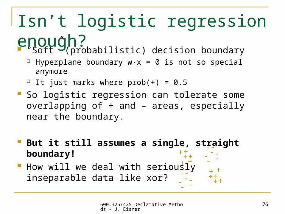
Isn’t logistic regression enough? “Soft” (probabilistic) decision boundary
Hyperplane boundary wx = 0 is not so special anymore It just marks where prob(+) = 0.5
So logistic regression can tolerate some overlapping of + and – areas, especially near the boundary.
But it still assumes a single, straight boundary! How will we deal with seriously
inseparable data like xor? ++
++
++
++
++
++
---
- --
-
---
- --
-

600.325/425 Declarative Methods - J. Eisner
77
The xor problem
(0 or 1)
> 0 ?
b=w0 w1 w2
x1 x2
(0 or 1)(always 1)
bias
A schematic way of showing how wx+b is computed. The red box outputs + or – according to whether wx+b > 0.
+++
++
+
++
++
++
---
- --
-
---
- --
-
0 1
0
1
x1
x2
Want to output “+” just when x1 xor x2 = 1.
Can’t be done with any w = (w0, w1, w2)!Why not?
If w is such thatturning on either x1=1 or x2=1 will push wx+b above 0,
then turning on both x1=1 and x2=1 will push wx+b even higher.

600.325/425 Declarative Methods - J. Eisner
78
The xor problem
(0 or 1)
> 0 ?
b=w0 w1 w2
x1 x2
(0 or 1)(always 1)
bias
A schematic way of showing how wx+b is computed. The red box outputs + or – according to whether wx+b > 0.
0 1
0
1
x1
x2
Want to output “+” just when x1 xor x2 = 1.
Can’t be done with any w = (w0, w1, w2)!Why not?
Formal proof: these equations would all have to be true,but they are inconsistent.
b < 0b+w1
> 0
b+w2
> 0b+w1+w2
< 0

600.325/425 Declarative Methods - J. Eisner
79
The xor solution: Add features
(0 or 1)
> 0 ?
b=w0 w1 w2
x1 x2
(0 or 1)(always 1)
bias
Want to output “+” just when x1 xor x2 = 1.
w3
x1 and x2
+++
++
+
++
++
++
---
- --
-
---
- --
-
0 1
0
1
x1
x2

600.325/425 Declarative Methods - J. Eisner
80
The xor solution: Add features
(0 or 1)
> 0 ?
b=w0 w1 w2
x1 x2
(0 or 1)(always 1)
bias
0 1
Want to output “+” just when x1 xor x2 = 1.
w3
x1 and x2
---
- --
-
+
++
++
+
++
++
++-
--
- --
-
0
1
x1
x2
x 1 an
d x 2
In this new 3D space, it is possible to draw a plane that separates + from -.

600.325/425 Declarative Methods - J. Eisner
81
The xor solution: Add features
slide thanks to Ata Kaban

600.325/425 Declarative Methods - J. Eisner
82
The xor solution: Add features
(0 or 1)
> 0 ?
-1 2 2
x1 x2
(0 or 1)(always 1)
bias
Want to output “+” just when x1 xor x2 = 1.
-5
x1 and x2
x1 and x2 drive the output positive.But if they both fire,
then so does the new feature,more than canceling out their combined
effect.
---
- --
-
+
++
++
+
++
++
++-
--
- --
-0 1
0
1
x1
x2
x 1 an
d x 2

600.325/425 Declarative Methods - J. Eisner
83
“Blessing of dimensionality” In an n-dimensional space, almost any set of up to n+1 labeled points
is linearly separable!
General approach: Encode your data in such a way that they become linearly separable.
Option 1: Choose additional features by hand. Option 2: Automatically learn a small number
of features that will suffice.(neural networks)
Option 3: Throw in a huge set of features like x1 and x2,slicing and dicing the original features in manydifferent but standard ways.(kernel methods, usually with SVMs)
In fact, possible to use an infinite set of features (!)

600.325/425 Declarative Methods - J. Eisner
84
Another example: The ellipse problem
32 22
21 xx
),2,(),( 2221
2121 xxxxxx
Not linear in the original variables.
Ellipse equation:
32 22
21 xx
),2,(),( 2221
2121 xxxxxx
But linear in the squared variables!Boundaries defined by linear
combinations of x2, y2, xy, x, and y are ellipses, parabolas, and hyperbolas in
the original space.

600.325/425 Declarative Methods - J. Eisner
85
Adding new features
Instead of a classifier w such that w.x > 0 for positive examples w.x < 0 for negative examples,
pick some function that turns x into a longer example vector, and learn a longer weight vector w such that
w.(x) > 0 for positive examples w.(x) < 0 for negative examples
So where does come from? Are there good standard functions to try? Or could we learn too?

600.325/425 Declarative Methods - J. Eisner
86
What kind of features to consider?
(0 or 1)
> 0 ?
-1 2 2
x1 x2
(0 or 1)(always 1)
bias
Want to output “+” just when x1 xor x2 = 1.
-5
x1 and x2
x1 and x2 drive the output positive.But if they both fire,
then so does the new feature,more than canceling out their combined
effect.
---
- --
-
+
++
++
+
++
++
++-
--
- --
-0 1
0
1
x1
x2
x 1 an
d x 2

600.325/425 Declarative Methods - J. Eisner
87
What kind of features to consider?
> 0 ?
-1 2 2
x1 x2bias
Want to output “+” just when x1 xor x2 = 1.
-5
x1 and x2
---
- --
-
+
++
++
+
++
++
++-
--
- --
-0 1
0
1
x1
x2
x 1 an
d x 2

600.325/425 Declarative Methods - J. Eisner
88
Some new features can themselves be computed by linear classifiers
> 0 ?
-1 2 2
x1 x2bias
Want to output “+” just when x1 xor x2 = 1.
-5
---
- --
-
+
++
++
+
++
++
++-
--
- --
-0 1
0
1
x1
x2
x 1 an
d x 2
-3
> 0 ?
2 2
Outputs 1 just when x1 and x2 = 1.

600.325/425 Declarative Methods - J. Eisner
89
Some new features can themselves be computed by linear classifiers
> 0 ?
-1 2 2
x1 x2bias
Want to output “+” just when x1 xor x2 = 1.
-5
---
- --
-
+
++
++
+
++
++
++-
--
- --
-0 1
0
1
x1
x2
x 1 an
d x 2
-3
> 0 ?
2 2
Like a biological neuron (brain cell or
other nerve cell), which tends to “fire” (spike in electrical output) only if
it gets enough total electrical input.
Outputs 1 just when x1 and x2 = 1.

600.325/425 Declarative Methods - J. Eisner
90
Some new features can themselves be computed by linear classifiers
Like a biological neuron (brain cell or
other nerve cell), which tends to “fire” (spike in electrical output) only if
it gets enough total electrical input.
Outputs 1 just when x1 and x2 = 1.
total input to a given cell
cell’s output
(usually
0 or 1)

600.325/425 Declarative Methods - J. Eisner
91
Architecture of a neural network

600.325/425 Declarative Methods - J. Eisner
92
Architecture of a neural network(a basic “multi-layer perceptron” – there are other kinds)
input vector x
output y ( 0 or 1)
intermediate(“hidden”) vector h
1x 2x 3x 4x
1h 2h 3h
y
Small example … often x and h are much longer vectors
Real numbers.Computed
how?

600.325/425 Declarative Methods - J. Eisner
93
Architecture of a neural network(a basic “multi-layer perceptron” – there are other kinds)
input vector x
22 wxh
1x 2x 3x 4x
2hintermediate(“hidden”) vector h
21w 22w 23w 24w
))exp(1/(1 22 wxh
0 if 1
0 if 0
2
22
wx
wxh
only linear
notdifferentiable

600.325/425 Declarative Methods - J. Eisner
94
youtput y ( 0 or 1)
1h 3h
Architecture of a neural network(a basic “multi-layer perceptron” – there are other kinds)
input vector x
intermediate(“hidden”) vector h
1x 2x 3x 4x
2h
))exp(1/(1 vhy
each hidden node is computed fromnodes below itin an identical way(but each uses different weights)
same for the output node
1v 2v 3v

600.325/425 Declarative Methods - J. Eisner
95
Basic question indifferentiating f:
For each weight (w23
or v3), if we increased it by , how much would y increase or decrease?This is exactly a Calc II question!
(What would happen to h1, h2, h3? And how would those changes affect y?Can easily compute all relevant #s top-down: “back-propagation.”)
y
Architecture of a neural network(a basic “multi-layer perceptron” – there are other kinds)
1x 2x 3x 4x
In summary, y = f(x,W) where f is a certain hairy differentiable function. Treat f as a black box.
input vector
collection of weight vectors
We’d like to pick Wto minimize (e.g.)
2
2
)),((
)(
Wxfy
yy
true
true
summed over all training examples (x,ytrue).
That is also a differentiable function.

600.325/425 Declarative Methods - J. Eisner
96
How do you train a neural network?
-3 -2 -1 0 1 2 3 4
collection W of all weights
erro
r o
f th
e n
etw
ork
ou
tpu
t The function optimizer will try to adjust w to drive error closer to 0.
Simulates a marble rolling downhill. Basic calculus to compute gradient.

600.325/425 Declarative Methods - J. Eisner
97
How do you train a neural network?
Minimize the loss function, just as before … Use your favorite function minimization algorithm.
gradient descent, conjugate gradient, variable metric, etc.
nasty non-differentiable cost function with local
minima
nice smooth and convex cost function: pick one of
these
Uh-oh …We made the cost function differentiable by using sigmoids
But it’s still very bumpy (*sigh*)You can use neural nets to solve SAT, so they must be hard

600.325/425 Declarative Methods - J. Eisner
98
The human visual system is a feedforward hierarchy of neural modules
Roughly, each module is responsible for a certain function
slide thanks to Eric Postma (modified)
Multiple hidden layers

600.325/425 Declarative Methods - J. Eisner
99
0 hidden layers: straight lines (hyperplanes)
slide thanks to Eric Postma (modified)
y
1x 2x
Decision boundaries of neural nets

600.325/425 Declarative Methods - J. Eisner
100
1 hidden layer: boundary of convex region(open or closed)
slide thanks to Eric Postma (modified)
y
1x 2x
Decision boundaries of neural nets(found this on the web, haven’t checked it)

600.325/425 Declarative Methods - J. Eisner
101
2 hidden layers: combinations of convex regions
slide thanks to Eric Postma (modified)
y
1x 2x
Decision boundaries of neural nets(found this on the web, haven’t checked it)

600.325/425 Declarative Methods - J. Eisner
102
Kernel methods Neural network uses a smallish number of learned
features (the hidden nodes). An alternative is to throw in a large number of standard
features: e.g., products of pairs and triples of the original features.
32 22
21 xx
),2,(),( 2221
2121 xxxxxx
),2,(),( 2221
2121 xxxxxx

600.325/425 Declarative Methods - J. Eisner
103
Kernel methods Neural network uses a smallish number of learned
features (the hidden nodes). An alternative is to throw in a large number of standard
features: e.g., products of pairs and triples of the original features. (Or quadruples, or quintuples …)
But this seems to lead to a big problem: With quintuples, 256 features about 1010 features. Won’t this make the algorithm really, really slow? And how the heck will we accurately learn 1010 coefficients (the
length of the weight vector w) from a small training set? Won’t this lead to horrible overfitting?

600.325/425 Declarative Methods - J. Eisner
104
Why don’t we overfit when learning 1010 coefficients from a small training set?
-3 -2 -1 0 1 2 3 4w.x
los
s (
if x
is
a
po
sit
ive
ex
am
ple
)
0-1 loss
perceptron
Initially, w = the 0 vector.If w(x) < 0, increase w by(x).
If w(x) > 0, w is working: leave it alone.
Remember the perceptron algorithm? How does it change w? Only ever by adding a multiple of some training example (xi). So w ends up being a linear combination of training examples! Thus, are we really free to choose any 1010 numbers to describe w? Not for a normal-size training set … we could represent w much more
concisely by storing each xi and a coefficienti . Then w = i i (xi).

600.325/425 Declarative Methods - J. Eisner
105
Why don’t we overfit when learning 1010 coefficients from a small training set?
Small training set less complex hypothesis space. (Just as for nearest neighbor.) Good!
Better yet, i is often 0 (if we got xi right all along). All of this also holds for SVMs.
(If you looked at the SVM learning algorithm, you’d see w was a linear combination, with i0 only for the support vectors.)
Remember the perceptron algorithm? How does it change w? Only ever by adding a multiple of some training example (xi). So w ends up being a linear combination of training examples! Thus, are we really free to choose any 1010 numbers to describe w? Not for a normal-size training set … we could represent w much more
concisely by storing each xi and a coefficienti . Then w = i i (xi).

600.325/425 Declarative Methods - J. Eisner
106
How about speed with 1010
coefficients? What computations needed for perceptron, SVM, etc? Testing: Evaluate w(x) for test example x. Training: Evaluate w(xi) for training examples xi.
We are storing w as i i (xi). Can we compute with it that way too? Rewrite w(x) = (i i (xi))(x)
= i i ((xi)(x))
So all we need is a fast indirect way to get ((xi)(x)) without computing huge vectors like (x) …

600.325/425 Declarative Methods - J. Eisner
107
The kernel trick Define a “kernel function” k(a,b) that computes ((a)(b)) Polynomial kernel: k(a,b) = (ab)2
example ellipsefor used we for the )()(
)2,,()2,,(
)2(
)()(),(
2122
2121
22
21
212122
22
21
21
22211
2
ba
bbbbaaaa
bbaababa
babababak
How about (ab)3 , (ab)4? What do these correspond to? How about (ab+1)2 ? Whoa. Does every random function k(a,b) have a ?

600.325/425 Declarative Methods - J. Eisner
108
What kernels can I use? Given an arbitrary function k(a,b),
does it correspond to (a)(b) for some ? Yes, if k(a,b) is symmetric and meets the so-called Mercer
condition. Then k(a,b) is called a “kernel” and we can use it. Sums and products of kernels with one another, and with
constants, are also kernels.
Some kernels correspond to weird such that (a) is infinite-dimensional. That is okay – we never compute it!We just use the kernel to get (a)(b) directly. Example: Gaussian Radial Basis Function (RBF) kernel:
)2/exp(),( 22
babak

600.325/425 Declarative Methods - J. Eisner
109
How does picking a kernel influence the decision boundaries that can be learned? What do the decision boundaries look like in the
original space? Curve defined by x such that w(x) = 0
for quadratic kernel, a quadratic function of (x1, x2 ,…) = 0
Equivalently, x such that i i k(xi,x)=0 where i > 0 for positive support vectors,
i < 0 for negative support vectors so x is on the decision boundary
if its “similarity” to positive support vectors balances its “similarity” to negative support vectors, weighted by fixed coefficients i .
x
+
+-
600.325/425 Declarative Methods - J. Eisner
110
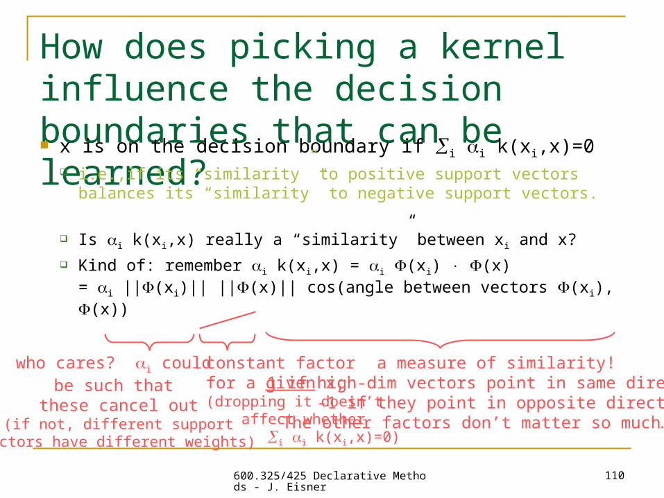
How does picking a kernel influence the decision boundaries that can be learned? x is on the decision boundary if i i k(xi,x)=0
i.e.,if its “similarity” to positive support vectors balances its “similarity” to negative support vectors.
Is i k(xi,x) really a “similarity” between xi and x?
Kind of: remember i k(xi,x) = i (xi) (x) = i ||(xi)|| ||(x)|| cos(angle between vectors (xi), (x))
a measure of similarity!1 if high-dim vectors point in same direction,
-1 if they point in opposite directions.The other factors don’t matter so much…
who cares? i could be such that
these cancel out(if not, different support
vectors have different weights)
constant factorfor a given x;(dropping it doesn’t affect whether i i k(xi,x)=0)

600.325/425 Declarative Methods - J. Eisner
111
Visualizing SVM decision boundaries … http://www.cs.jhu.edu/~jason/tutorials/SVMApplet/ (by Guillaume Caron)
Use the mouse to plot your own data, or try a standard dataset Try a bunch of different kernels
The original data here are only in 2-dimensional space, so the decision boundaries are easy to draw.
If the original data were in 3-dimensional or 256-dimensional space, you’d get some wild and wonderful curved hypersurfaces.