145

6 Analyzing pulse amplitude

modulation (PAM)

fluorometry curves of intact

chloroplasts

This chapter is based on a manuscript in preparation.

Joris J. Snellenburg, Matthew P. Johnson, Alexander V. Ruban, Rienk van Grondelle,

Ivo H.M. van Stokkum

146

6.1 ABSTRACT

Pulse amplitude modulation (PAM) fluorometry is used extensively to probe changes in

Photosystem II (PSII) turnover rate as a result of changing light conditions. Utilizing the

saturation pulse method the phenomenon of non-photochemical quenching (NPQ) is

assessed through so called quenching analysis curves, obtained on spinach chloroplast.

We present an analysis method which describes the observed fluorescence quantum yield

in these curves as the sum of the product of dynamically changing concentrations of

different emissive species and their fluorescence quantum yields. Specifically we show

that the observed yield can largely be described by PSII operating in one of four distinct

states, quenched or not quenched, both either open or closed depending upon the QA

reduction. In this way we were able to demonstrate that after a period of recovery

following a period of quenching inducing actinic light some of the RCs remain permanently

closed (about 1/12 after one cycle, 1/6 after two cycles). Quenching is also larger after the

second cycle, due to recovery from quenching occurring on two time scales, with rates of

(50s)-1 and (1h)-1. The analysis method presented here is flexible, allowing it to be applied

to any type of PAM fluorometry protocol, including those routinely used for plants in

greenhouses or crops in the field. It provides a way to quantitatively compare qualitatively

different PAM curves on the basis of statistically relevant fitting parameters rather than

just by visual inspection.

147

6.2 INTRODUCTION

Pulse amplitude modulation (PAM) fluorometry is a technique which can be used to

measure the fluorescence quantum yield even in the presence of actinic light (Schreiber

2004; Schreiber et al. 1986), and as such can be performed in a wide range of

physiological conditions. The required equipment is relatively inexpensive and can even

be carried into the field (Bilger et al. 1995).

The fluorescence detected by a PAM fluorometer originates from all pigment-protein

complexes that absorb light at the excitation wavelength used and emit fluorescence

overlapping with its detector window (typically λ > 700 nm). Modulation is used to ensure

that the recorded signal is due to the (constant) modulated measuring light only. Any

increase or decrease in the recorded signal can directly be related to changes in the

fluorescence quantum yield of the different pigment protein complexes.

In a top-down approach, theoretical models of the light dependent reactions in the

thylakoid membrane can predict a PAM signal, which can be used to verify such models.

The (fast) kinetics of chlorophyll fluorescence induction is described in e.g. (Vredenberg

2000; Ritchie 2008; Schansker et al. 2011) reviewed in (Lazár and Schansker 2009; Rubin

and Riznichenko 2009) and more recently (Belyaeva et al. 2016). The slower processes

such as non-photochemical quenching (NPQ) and state transitions, are modelled in

(Ebenhöh et al. 2011; Zaks et al. 2012; Ebenhöh et al. 2014; Matuszyńska and Ebenhöh

2015; Matuszyńska et al. 2016).

Here we adopt a bottom-up approach (Acuna et al. 2016), analyzing the PAM signals of

various intact chloroplasts obtained using a typical light protocol used for quenching

analysis experiments, and quantify the dynamically changing concentrations of the

different emissive species. In our approach we explicitly assume a discrete number of

states for the contribution of Photosystem II (PSII). It can be quenched or unquenched and

switches between these extremes due to changes in the actinic light. At the same time it

can be open or closed dependent on the reduction state of the QA site of the PSII RC,

resulting in a total of four discrete states for PSII. Apart from PSII which dominates the

signal there are other emissive species that contribute to the measured fluorescence

quantum yield, e.g. PSI (Peterson et al. 2014; Schansker et al. 2005), disconnected

antenna complexes such as light harvesting complex I and II (LHCI and LHCII (Belgio et al.

2012) respectively). The relative concentrations and the measured quantum yields of

different emissive species depend on the organism, growing conditions, mutations,

chemical treatments, etc. We employ a parametric model which takes the light protocol

and the high quality measurements as input and aims to describe the data up to the noise

level, in order to extract all the information available. The method is flexible enough to

148

analyze multiple measurements (e.g. different preparations, different mutations)

following the same protocol simultaneously, while linking parameters between datasets

that are expected to be conserved, i.e. global analysis of PAM fluorometry data. In this

way it is possible to more reliably quantify differences in photosynthetic efficiency or

stoichiometry of the photosynthetic complexes between experiments. To illustrate this

point, measurements on intact chloroplasts, prepared in a way that they were either

devoid of zeaxanthin (V) or enriched in zeaxanthin (Z), are used as test cases throughout

this paper.

Figure 6.1 lists the different emissive species that may be encountered in this case. Each

species is associated with a particular relative quantum yield Φ which will be estimated

from the PAM quenching analysis curves. In the appendix it will also be demonstrated for

the V and Z preparations how some of these quantum yields can also be independently

estimated from picosecond time-resolved fluorescence measurements.

Figure 6.1: Overview of the different emissive species that can contribute to a measured

PAM curve for plants and green algae. The Photosystem II supercomplex can occur in four

different states depending on whether the RC is open (o) or closed (c), and the complex as

a whole is being quenched non-photochemically (q) or unquenched (u). The states are

duplicated between the two different samples (V, Z) to emphasize that the yields may be

different. Photosystem I can contribute but is assumed to be unaffected by quenching or

saturating light conditions. Disconnected LHCII can also contribute and is assumed to be

affected by quenching in the same way as PSII. Under normal conditions it is only present

in negligible amounts.

Thus our bottom-up approach does take into account the biophysical origin of the

emitting states which can interconvert, but describes the dynamics phenomenologically,

149

i.e. with exponential decays. In the discussion we will close the loop, and connect to a top-

down theoretical model. The predictions from such a model can be quantitatively

compared to the results from our parametric description, and thus inspire the iterative

improvement of the top-down theoretical model.

6.3 EXPERIMENTAL DATA

Figure 6.2 shows three measured PAM fluorescence quenching curves obtained on dark

adapted intact spinach chloroplasts either devoid (black curve) of, or enriched in

zeaxanthin (red and blue curves), labeled respectively the “V”, “Z” and “GA” dataset. The

relative chlorophyll fluorescence quantum yield is probed over a period of 25 minutes

with 60 millisecond sampling intervals while subjected to a complex actinic light protocol

controlling the actinic background light and saturating flashes. The GA dataset

represented by the blue curve in Figure 6.2 is similar to the Z dataset, except that around

t≈410s glutaraldehyde was added, largely inhibiting recovery from quenching. The same

data was presented in Figure 1A of (Johnson and Ruban 2009). A brief description of the

materials and experimental procedures under which these curves were obtained can be

found in the supporting information (SI) accompanying this manuscript. The light protocol

can be used to distinguish a number of light regimes (LR0 – LR6), indicated in the

white/gray/yellow bar in Figure 6.2. In the first 30 seconds (LR0: 0.02s – 30.02s; white) a

background signal is measured. Then the measuring light is switched on while the actinic

light is still switched off (LR1: 30.08s – 124.94s; gray), probing the minimal variable

fluorescence level in the dark, typically labeled Fo and associated with completely open

PSII RCs. Periodically a saturating pulse of light (0.8s; 4000 μmol m-2 s-1) is applied

(indicated by a black stripe on top of the bar in Figure 6.2) probing the maximal level of

variable fluorescence, typically labeled Fm when the sample is dark adapted and labeled

Fm’ when the sample is under the influence of actinic light, and associated with

completely closed RCs. During the initial period of darkness two such saturating pulses are

applied and some recovery dynamics following the saturating pulse is observed. The next

phase of the experiment consists of a period of actinic light (level = 350 μmol @635 nm)

(LR2: 125.0 – 429.98; yellow) in which fluorescence quenching in the form of a steady

decline of the fluorescence yield is observed, followed by a period of darkness (LR3:

429.98 – 740.0; gray) where the fluorescence (partially) recovers to the levels of the dark

adapted state. A second period of actinic light (LR4: 740.06 – 1045.1; yellow) is again

followed by a period of darkness (LR5: 1045.16s – 1350.02s; gray) showing somewhat

different dynamics, before the measurement light is again switched off (LR6: 1350.08s –

1354.94s, white). Thus, the whole measurement can be divided into a number of discrete

segments starting at the moment of a change in light conditions (measuring light on or off,

actinic light on or off, saturating pulse on or off) and ending the moment in time just

before another change is observed. For these data this amounts to 77 unique segments.

150

The beginning of each segment can be determined from the data by visual inspection, it

can be estimated during the analysis, or, ideally, it can be automatically generated from

the experimental protocol that was used to record the data. In each segment the data are

fitted with a unique model function defined with respect to the start of the segment (time

zero; t0), while all model functions share a common parameter set.

Figure 6.2: PAM fluorescence quenching / induction curves obtained on intact Chloroplasts

devoid of zeaxanthin (black), enriched in zeaxanthin (red, blue) using the saturating pulse

method. Alternating darkness (dark adaptation, recovery, indicated by a gray bar above

the curve) and continuous actinic light (inducing quenching, yellow bar) to measure

quenching induction/recovery while periodically probing the maximal level of fluorescence

with saturating pulses (indicated by stripes in the top of the graph). The blue curve

represents a sample where glutaraldehyde was added (at t≈410s) to prevent the recovery

from the quenched state. The black curve was normalized to the maximum of the

fluorescence in darkness, and the red and blue curves were then scaled to the minimal

level of fluorescence in darkness of the black curve. Measuring light and actinic light of 620

and 635 nm respectively was used, and fluorescence was detected above 700 nm.

6.4 CONSTRUCTING A PARAMETRIC MODEL

To create a parametric description of our experimental data, we start by recognizing that

the experimental data is the result of a PAM fluorometer running a complex light protocol

while sampling the fluorescence quantum yield with high resolution. The protocol

specifies exactly when and for how long the sample is exposed to a certain intensity

151

(ranging from high to none) of actinic light and additionally when and for how long

saturating flashes are given. The signal that is measured depends on the stoichiometry of

the species probed with the PAM measuring light, as well as their specific quantum yield

which, in the case of PSII, can strongly depend on the actinic light conditions. While the

sum of concentration of species may be constant, their stoichiometry certainly isn’t. In

this case study we consider four states of PSII: it can be open or closed and it can be part

of a quenched or unquenched complex (see Figure 6.1). PSII is considered closed when the

QA site is reduced. We will return to the consequence of ignoring the PSI contribution in

the discussion. Figure 1.6 summarizes the method of analysis of PAM curves using a

parametric model, subsequently every aspect will be discussed in more detail.

Figure 6.3. PAM analysis method using a parametric model. A sample (of in this case intact

chloroplasts devoid of zeaxanthin) is measured following a specific light protocol consisting

of regimes of quenching inducing continuous actinic light, recovery regimes with no actinic

light, and saturating pulses throughout the experiment. The resulting data as well as the

light protocol form the input for a parametric model which results in a description of the

data in terms of a number of species concentrations C and their quantum yields Φ .

In order to construct a parametric model that can be used to fit and quantitatively

describe PAM fluorometry curves the following assumptions are made. 1) The total

measured fluorescence quantum yield can be described as the linear combination of the

concentrations of a number of emissive species j and their quantum yields Φ�. 2) The

quantum yields of these species are independent of their relative concentration or

experimental (lighting) conditions.

152

A species is then defined as a pigment-protein complex which can be excited by the

measuring light of the PAM fluorometer and which has a unique spectral and kinetic

signature of excited state decay resulting in a specific contribution to the emission in the

integration window of the PAM fluorometer (see also Figure 6.1). The concentrations of

the different species can change dynamically when one species is interconverted into

another, in which case the sum of the concentrations can be assumed to remain constant.

For instance if the process of closing PSII RCs by applying a saturating pulse can be

described with f(x) the concentration of open PSII is described with (1-f(x)). In extreme

measuring conditions species could get photoinhibited resulting in a decrease in the sum

of concentrations. The dynamics of the concentrations as a function of the measurement

time Ct is dependent on the light conditions of the experiment and can be parameterized

with a parameter vector P, which is independent of the species specific quantum yield Φ .

The total PAM signal J, decomposed into j species, can then be written as:

( ) ( ), ,PAM ( ); ,x j x j x

t kl kljkl

J C tΦ = ⋅Φ∑C P P 1

where the additional indices k and l represent different light–acclimated states; e.g. in the

case of PSII k takes into account whether the state is open or closed and l stands for either

a quenched or an unquenched species The label x is used to represent the state of

zeaxanthin enrichment, e.g. V in the case of a sample devoid in zeaxanthin and Z in the

case of the sample enriched in zeaxanthin.. Enumerating over all species j for state x

(where x equals V or Z) we get:

PSII,x PSII,x PSII,x PSII,x PSII,x PSII,x PSII,x PSII,xxPAM ou ou cu cu oq oq cq cqJ C C C C= ⋅Φ + ⋅Φ + ⋅Φ + ⋅Φ 2

Taking the assumption of a limited number of discrete states (Figure 6.1) substituted into a

parametric model (equation 1 and Figure 6.3) resulting in equation 2 we arrive at our

working model depicted in Figure 6.4. Here the dynamics of the concentrations PSII,x PSII,x PSII,x PSII,x, , ,ou cu oq cqC C C C is captured by a limited number of rate constants (k1, k2, etc),

reflecting the interconversion of one state in the system to another. For instance k1 (in a

saturating pulse) or k10 (under actinic light) reflect the rates in which open unquenched PSII

is converted to closed unquenched PSII, subsequently k4, k4a and k5 reflect the three rate

constants needed to describe the quenching of PSII under the continued influence of actinic

light (indicated by a red arrow). Returning to darkness the re-opening of the RC is

described by k2, k3 and k3b and the recovery from quenching by rates k8 and k8a which occur

in the absence of light as indicated by the blue arrows.

153

Figure 6.4. Working mathematical model which ties the different species listed in

Figure 6.1 to the parametric description given in equation 1. The premise of the model are

four distinct states which can be interconverted into one another with certain rates, either

light driven (red arrows) or spontaneously in the absence of light (blue arrows). To simplify

the model it was assumed that during the course of the experiment the concentration of

zeaxanthin remains constant so that species only interconvert within the front plane

defined by a certain fixed level of zeaxanthin.

The amplitude fractions (how much decay can be ascribed to a particular rate constant)

have been omitted from the figures for the sake of brevity, but are discussed below.

Detailed considerations are described in the SI, section “Components of a parametric

model for PAM curves”, which also lists the complete set of equations used for the total

154

fitting function. To simplify the model, we assume that the concentration of zeaxanthin

remains constant throughout the course of the experiment, as adding this complexity

would add a third dimension to the model whereas the fitting results show that given the

short duration of the experiments this extra complexity is not needed to adequately

describe the data.

6.5 SIMULATING PAM FLUOROMETRY CURVES

Using the function definition of equation 2 the quenching analysis curves can either be

simulated using any chosen set of parameters or fitted directly to the measured data from

Figure 6.2. To illustrate the different aspects of the model, a simulation is performed with

parameters which are in good agreement with those needed to describe the

measurements of zeaxanthin enriched chloroplasts (red curve, Figure 6.2). See Figure S

6.2 for an impression of the implementation of the simulation. Note that in the screenshot

the contributions from species other than PSII (e.g. PSI) have been set to zero in this

simulation. The first part of the simulation consists of a brief period of darkness, with two

saturating pulses, and then a period of quenching inducing high light; this is shown in

Figure 6.5. The recovery period that follows the period of continuous actinic light is shown

in Figure 6.6. For comparison the measured data is shown by gray dots and the simulated

trace in solid black. The residuals, defined as data minus simulation, are shown in light

gray. Given the noise level of the data (standard deviation is < 0.01) it is clear from the

residuals of this simulation that the model is not perfect but all essential features of the

data are captured, which will be discussed below.

The simulation starts with 30 seconds of background signal (ML off). When the ML is

turned on (but the actinic light is still off), the signal instantaneously (in less than the 60

ms step size) reaches a level of minimal variable fluorescence, which can be written as the

product of a time dependent (but in this case constant) concentration function and a

constant quantum yield (the same throughout the simulation): ( )PSII PSIIou oucJ t= ⋅Φ (where

ou indicates that the RC is open and the complex as a whole is unquenched), with in this

case ( )PSIIouc 1t = , PSII

ou 0.21Φ = . Note that this quantum yield is not absolute but relative to

the chosen normalization in Figure 6.2. During this period of relative darkness (only ML) at

two moments in time (tSP1=61.40; tSP2=115.34) a saturating pulse of about 0.8s is applied,

which is assumed to quickly close all PSII RCs, but not induce any quenching. This

translates to a full conversion of the concentration of open unquenched PSII to closed

unquenched PSII. The expression that captures this can be written as:

( )0 01 1PSII PSII( )ou cu

( )e e1

k t t k t tJ

− − − −= ⋅Φ + − ⋅Φ where -11 9.4sk = , PSII

ou 0.21Φ = as before,

PSIIcu 0.67Φ = and where in lieu of t0 either tSP1 or tSP2 is substituted. After the saturating

155

pulse the subsequent reopening of the closed PSII RCs is modeled using a sum of three

exponentials that describes the conversion of closed unquenched PSII back into open

unquenched PSII.

( )( ) ( )PSII PSII PSII PSIIou cu1 cl clJ c t c t= − ⋅Φ + ⋅Φ with

( ) 12 0 3 0 3 0PSII

2 3 3b( ) ( ) ( )

e e eD

b

c

k t t k t t k t t

lc t a a a− − − − − −+= + where

-1 -1 -12 3 3b9.4s , 0.002s , 0.16sk k k= = = , 2 3 3b0.65, 0.06, 0.29a a a= = = for SP1 and

2 3 30.81, 0.03, 0.16ba a a= = = for SP2. The recovery after the very first saturating pulse in

darkness is slower than that after subsequent saturating pulses.

Figure 6.5: Simulated PAM curve of intact spinach chloroplasts enriched in zeaxanthin.

Legend: data (gray), simulation (black), residual (light gray, straddling the zero line). The

bottom half of the color bar indicates the light condition (white: no ML, gray: only ML,

yellow: ML and actinic light). The upper half indicates when a SP was applied. The inset

represents a zoom of the second saturating pulse in darkness. The inset labels indicate

which of the rates ki from Figure 6.4 apply to which segments in the data. Further details

are discussed in the text.

Following the period of relative darkness, as indicated by the gray bar in Figure 3, is a

period of continuous actinic light, indicated by a yellow bar. The moment the actinic light

is switched on (tLR2) the fluorescence level is observed to rise due to the closing of all PSII

RCs, which is again approximated with a single exponential rise. However, the maximum

156

level of fluorescence yield reached is somewhat lower than during the saturating pulses in

darkness, which is modelled here by the immediate onset of a fast quenching process.

This means that at this point all states of PSII as illustrated in Figure 6.1 can occur

simultaneously. For simplicity we only describe the contribution of PSII in the closed and

quenched state, by far the dominant component during the period of actinic light, which

can be written as the product of a closing function and a quenching function times the

relevant quantum yield:

( ) ( )( )( )( )

( ) ( ) ( ) ( )( )pLR

10 0

4 pLR 5 pLR

quenching

closing

SQPSII PSIIcq cq

SQ 4 4

1 e1 1 e *

1 e 1 e

SQk t t

k t t

D D k t t k t t

frJ cl cl

fr a a

− −

− −− − − −

− − = + − − Φ − + −

�������������������

�������������

Here clD=0.09 represents a fraction of the total PSII population which is (still) closed, due

to the remaining effect of a preceding saturating pulse, and defined as the function PSIIclc

evaluated at the last timepoint in darkness . The conversion of PSII in the open state to

the closed state occurs with a rate of k10=10/s, and t0 is substituted with the start of the

actinic light regime (tLR2=125s). Quenching is divided into two fractions which differ in

their rate of recovery. A slow-to-recover quenching fraction SQ 0.27fr = rises with a rate

kSQ=0.07s-1. A quick-to-recover fraction ( )SQ1 0.73fr− = rises on two timescales, a small

fraction 4 0.22a = rises relatively slowly with a rate of k4=0.01/s and a fraction

( )41 0.78a− = rises with rate k5=0.1/s. The full expression can be found in the SI, but in

principle it is easily derived since the concentration of PSII in the open state is (1 )closed−

, and the amount of unquenched PSII is (1 )quenched− . The full expression also takes into

account that a fraction of the PSII can re-open during the course of actinic light

illumination, when the excitation pressure from the actinic light is not enough to keep all

PSII RCs closed. In this simulation it is assumed that all RCs are continually closed (

CC 1fr = , see SI) during actinic light because of the absence of a fluorescence increase

upon a saturating pulse during the period of actinic light.

After a period of actinic light follows a period of darkness during which the sample can

recover from quenching as shown in Figure 6.6. The initial effect of switching from actinic

light to relative darkness is re-opening of the PSII RCs, exactly as would happen after a

saturating pulse. Then on a longer timescale the sample also recovers from the quenching

induced by the actinic light, a fraction recovering quickly and the rest so slowly that at the

end of the recovery period a large part of it still hasn’t recovered, as can be observed in

Figure 6.2. For simplicity we describe here only the contribution of PSII in the open

157

unquenched state, which describes the baseline level during a recovery period. Again the

other contributions can easily be derived from this expression but for the complete

expression the reader is referred to the SI. The contribution of PSII in the open and

unquenched state to the total measured PAM signal J during recovery then becomes:

( )( )( )( )

( )( )

( ) ( )( )( )( )

2 0

8 pLR

3 0

3b 08a pLR

openingfast_recovery

2

SQ f f

3 slow_recovery

3bSQ s s

1 e1 1 1 e

1 e

1 e1 1 e

k t tk t t

k t tPSIIou

k t tk t t

afr QT QT

J a

afr QT QT

− −− −

− −

− − − −

− + − − + − = − + − + − + −

���������

�����������������

������������ �

PSIIou

Φ

��

where -1 -1 -12 39.4s , 0.16s , 0.002sk k k= = =

3b, 2 3 3 SQ0.81, 0.13, 0.06, 0.27ba a a fr= = = = .

The variables QTf and QTs represent how much quenching was induced during the

preceding period of actinic light for the fast-to-recover fraction and the slow-to-recover

fraction respectivelyIn this simulation QTf≈1, QTs≈1. The rates k8=0.02/s and k8a≈1/hour

are the rates of recovery for the fast and slow fraction respectively. The parameters a2, k2,

a3, k3, a3b, k3b, in principle are linked between the initial period of darkness and the period

of recovery, meaning that the dynamics of re-opening, following a saturating pulse in

darkness or actinic light, or the re-opening after switching off the actinic light, is treated in

the same way.

158

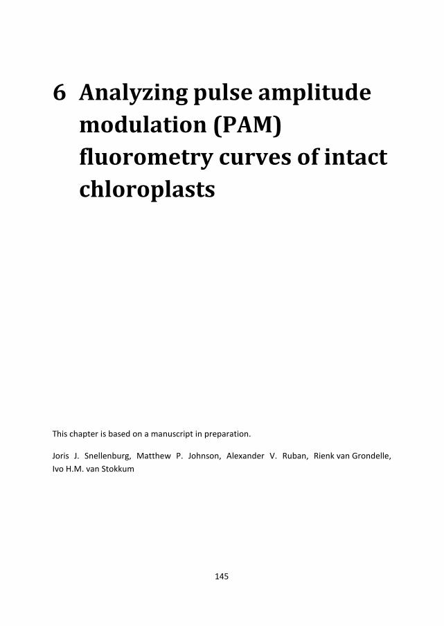
Figure 6.6: Simulated PAM curve representing the recovery region following a period of

actinic light as in Figure 6.5. The simulated trace is in solid black, the observations are

represented by dark gray dots. In light gray dots (straddling the zero line) are the residuals.

The inset labels indicate which of the rates from Figure 6.4 apply to which segments in the

data.

In general linking the parameters between the different segments is an a priori

assumption that fits well, however in the case that the dynamics are clearly observed to

be different, additional labeled parameters can be introduced, e.g. 12Rk where the label R1

indicates that the parameter is defined specifically for the first recovery regime. In the

same way D1 can be used for the first period of darkness, H1 for the first period of actinic

light, H2 for the second, etc.

The values of the estimated parameters, i.e. four estimated quantum yields, seventeen

rate constants and ten amplitude fractions are collated in Table 6.1.

159

PSIIoqΦ

PSIIouΦ

PSIIcqΦ

PSIIcuΦ

D1

1k

H11k

1

10Dk

H110k

D12k

D13bk

D13k

V 0.185 0.205 0.409 1.000 20 20 9.3 16 0.41 0.0441 Z 0.152 0.209 0.234 0.671 9.5 - 11 9.9 0.19 0.0238 GA 0.159 0.207 0.231 0.701 9.4 - 24 9.5 0.16 0.021 Z+GA 0.162 0.209 0.233 0.684 9.5 - 13 9.8 0.19 0.0244 H1

2k 1

4Hk

H1SQk

1

5Hk

24Hk

25Hk

H16k

26Hk

R18k

R18ak

V 35 0.050 0.0041 0.132 0.14 0.02 0.027 H16k

0.038 0.0002

Z - 0.008 0.061 0.105 0.02 0.21 - - 0.020 0.0005 GA - 0.089 0.0052 0.1 - - - - 0.000 0.0005 Z+GA - 0.006 0.048 0.12 0.02 0.20 - - 0.019 0.0002 H1

CCfr H1

SQfr

D12fr

D13bfr

SP12fr

SP13bfr

R22fr

R23bfr

H14fr

H24fr

V 0.91 0.46 0.81 0.53 0.78 0.54 0.75 0.52 0.77 0.78 Z 1.00 0.27 0.79 0.73 0.66 0.62 0.75 0.64 0.22 0.24 GA 1.00 0.14 0.81 0.73 0.66 0.65 0.39 0.80 0.93 0.24 Z+GA 1.00 0.28 0.80 0.75 0.66 0.62 0.73 0.68 0.18 0.24 Table 6.1. Parameter values estimated using non-linear regression. Four quantum yields, seventeen rate constants and ten fractional

amplitude parameters are given. For more information on the nature of each parameter the reader is referrred to Table S 6.1 and the

corresponding section in the SI. The relation between the fractional amplitude parameters and the amplitude parameters reported in the

main text is given in Table S 6.2. Parameters fixed during regression are indicated in bold. Parameters that were not relevant for a given

case are marked with '-'. The value of R18k listed for the Z+GA case applies to the Z dataset only, for the GA dataset it was fixed to 0

(there is no recovery from quenching in this case).

160

6.6 CALCULATING DERIVED QUANTITIES

With a completely parameterized description of the PAM curve in place, the next step is

to derive insightful quantities that have proven to be useful in prior PAM studies. For

instance NPQ is often expressed as (Fm/Fm’-1), where Fm is the maximal fluorescence

during a saturating pulse in darkness, or alternatively the maximum reached directly after

switching on actinic light after a period of dark adaptation, and Fm’ the maximal

fluorescence reached in a saturating pulse during actinic light exposure. In the context of

the functions listed in Table S 6.1 and defined in the SI, Fm can be defined as the

maximum of the functions labeled “dkspR” or “dk2hl”, and Fm’ can be defined as the

“hlspD” function evaluated with all decay rates set to zero (so that the level stays at the

maximum of the “hlspR” function). In the recovery period instead of “hlspD” the function

“recspD” is used instead. In Figure S 6.3 the NPQ curves for all datasets are visualized.

However note that the interpretation of the NPQ quantity, and especially the fitting

thereof is not without controversy (Holzwarth et al. 2013). Thus, it is more interesting to

directly visualize the individual contribution of each species (or in this case, each state of

PSII) to the total signal. This decomposition is visualized for the Z dataset in Figure 6.7 and

Figure S 6.5. In Figure 6.7 the concentrations of the four different states of PSII are shown

as a function of the measurement time, at any given moment summing up to a total

concentration of 1. In Figure S 6.5 the contribution of each state to the total quantum

yield (overlaid in gray dots, maximum 0.69) is shown. The black curve represents the sum

over the product of concentration and quantum yield for all four states (see table inset).

161

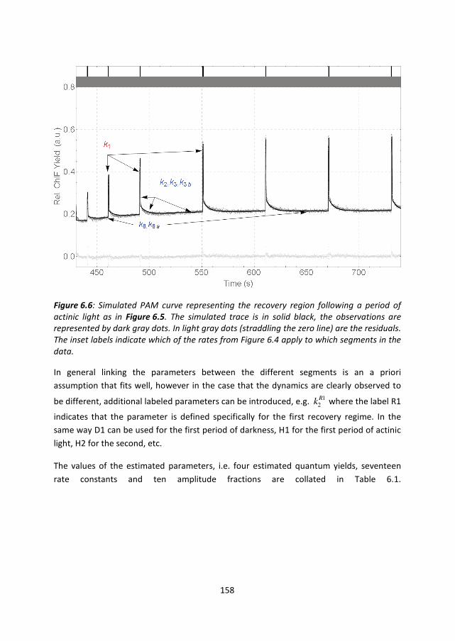
Figure 6.7: Concentration profiles of the different states of PSII contributing to the total

measured relative chlorophyll fluorescence quantum yield for the Z dataset. The sum of the

concentrations, open unquenched PSII (green, PSIIou 0.209Φ = ), closed unquenched PSII

(orange, PSIIcu 0.671Φ = ), open quenched PSII (blue,

PSIIoq 0.152Φ = ) and closed quenched

PSII (red, PSIIcq 0.234Φ = ) multiplied by their respective quantum yields result in the fitted

PAM curve depicted in solid black. For comparison the Z observations are overlaid as gray

dots. Light conditions are indicated by the top bar as described in the caption of Figure 6.2.

In the beginning, the contribution of PSII open unquenched (green curve) is maximal. At

the first saturating pulse this concentration drops to zero and the contribution of PSII in

the closed unquenched state (depicted in orange) is maximal. After the saturation pulse is

completed (0.8s after the onset) the concentration of closed unquenched decays back into

open unquenched. Just before the next saturating pulse the level is still not yet at the

level of Fo in darkness indicating that a small fraction (≈5%) is still closed. When the actinic

light is switched on (indicated by a yellow bar) the concentration of PSII closed quenched

is observed to quickly rise (red curve) at the expense of the closed unquenched state.

After switching the actinic light off again the fourth species enters, open quenched PSII

(blue curve). The lowest level in the data (well below Fo in darkness) largely determines PSIIoqΦ . During the recovery from quenching the quenched concentrations (red/blue) are

gradually replaced by unquenched (orange/green), but not completely. A substantial

amount (≈20%) of open quenched PSII (blue) remains, even after 300s of recovery. This is

162

a direct consequence of the observation in the data (cf. the red curve in Figure 6.2) that

the level of Fm’ at the end of the recovery period is substantially lower than Fm in

darkness. The same holds true for the maximum level reached upon turning on the actinic

light after the first recovery period. This accumulation of a slow-to-recover quencher is

described by the remaining concentration in the blue curve. But despite this incomplete

recovery from quenching, the baseline level of fluorescence in the data is even slightly

higher than the level of F0 in the initial period of darkness. Considering that the yield of

open quenched PSII lies below that of open unquenched PSII, there has to be a certain

fraction of closed quenched and closed unquenched PSII left which is seen as a non-zero

amplitude of the red and orange curves toward the end of the recovery periods. This

permanently closed fraction visible in Figure 6.7 is 7% after the first recovery period, and

11% after the second period of actinic light. This effect is even more clearly visible in the

decomposition of the V dataset, shown in Figure 6.8 (concentrations) and Figure S 6.6

(contributions), where the baseline level of F0 following a period of recovery is

substantially higher than during the initial period of darkness, and the accumulation of the

slow-to-recover quencher and the fraction of permanently closed PSII is even more

pronounced. Here the permanent closed fraction is 8% after the first recovery period, 17%

after the second recovery period.

Figure 6.8: Concentration profiles of the different states of PSII contributing to the total

measured relative chlorophyll fluorescence quantum yield for the V dataset. The sum of

the concentrations, open unquenched PSII (green, PSIIou 0.205Φ = ), closed unquenched PSII

163

(orange, PSIIcu 1.0Φ = ), open quenched PSII (blue,

PSIIoq 0.185Φ = ) and closed quenched PSII

(red, PSIIcq 0.409Φ = ) multiplied by their respective quantum yields produce the PAM curve

depicted in solid black. For comparison the V observations are overlaid as gray dots. Light

conditions are indicated by the top bar as described in the caption of Figure 6.2.

The main difference between Figure 6.7 and Figure 6.8 is the re-opening of a small

fraction of PSII RCs during actinic light. This is directly observed in the data as well: during

actinic light upon application of a saturating pulse the observed yield is slightly higher still.

This is now visualized in Figure 6.8 as the blue concentration, which slowly rises (it is

assumed that the initial switching on of the actinic light first closes everything) and which

drops to zero every time a saturating pulse is applied. As a consequence the concentration

of red/orange features a small spike which lasts only for the duration that the saturating

pulse is applied. In contrast to the period of darkness and recovery, where the actinic light

is on, the decay of the extra closed concentration is extremely fast under the influence of

actinic light. Another relevant difference is that the quenching level reached after the

second period of actinic light is substantially lower than after the first period, which is

explained by a quenched fraction which takes longer to form and is slow-to-recover.

The decomposition of the GA dataset is shown in Figure S 6.4 (concentrations) and Figure

S 6.7 (contributions).

6.7 FITTING PAM CURVES

Instead of mimicking the data by adjusting the parameters by hand, the parameters can

also be estimated using any non-linear regression method. The implementation in this

paper was constructed in Wolfram Mathematica, but the expression could easily be

ported to any other language or platform which has non-linear solvers available, such as

Matlab, Python, R or C++.

164

Figure 6.9 shows the fitted PAM curves for the V and Z datasets following optimization of

the parameters using non-linear regression. The V data is plotted in gray dots, the fit in

solid black, and the residual light gray. The Z data is shown in orange dots, the fit in solid

red and the residuals in dark gray.

Figure 6.9: Fitted PAM curves for the V and Z dataset where non-linear regression was

used to estimate the parameters (estimated values in Table 6.1). Estimated relative

quantum yields (relative toPSII,Vcu 1Φ = ) collated in the inset table. Data, fit and residuals

(straddling the zero line) for the V and Z dataset respectively shown in: gray dots, solid

black, light gray dots, and orange dots, solid red and dark gray dots. Light conditions

indicated by the top bar as described in the caption of Figure 6.2.

Not all parameters were set to be free parameters of the fit. In the case of the V dataset

the quantum yield of PSII in the closed unquenched state is fixed to 1 by definition, since

the data was normalized to the maximum of the first saturating pulse, where the only

contribution is assumed to be closed unquenched PSII. In the Z dataset, because the

saturating pulses during actinic light don’t result in an increased yield, the parameter

relating to the amount of continuously closed PSII in actinic light ( CCfr ) was fixed to 1,

which automatically means that the rate constant related to partial re-opening ( 6k ) could

be eliminated from the list of parameters to be optimized. Instead in the V dataset the

fraction was a free parameter of the fit and could be fitted ( CC 0.9fr = ), and the rate of

165

partial re-opening was found to be -6

10.03sk = . In addition it was found that the fraction

of slow-to-recover quenching ( H1SQfr ) was found to be substantially larger in the V dataset

(0.46) than in the Z dataset (0.27) (see Table 6.1). It is this large value of H1SQfr which

explains the relatively large difference between Fm during the initial phase of darkness

(1.0) and Fm’ at the end of the second recovery phase (Fm’=0.75), and at least partially

the difference between Fm’ at the end of the second and the first period of recovery

(Fm’=0.85). Recently, a similar slow to recover quenching effect was attributed to plant

‘memory’ (Matuszyńska et al. 2016), although there it was primarily related to the

accumulation of zeaxanthin.

In Figure 6.9, the parameters for the V and Z dataset were optimized for each dataset

separately, but the real power of having a parameterized description of the PAM curve is

when multiple datasets are analyzed with a shared set of parameters, i.e. global analysis

of PAM fluorometry data. A straightforward application is when several repeats of a

specific protocol are measured on the same sample. Rather than averaging the repeated

measurements, they could all be analyzed with a single model with a shared set of

parameters. These parameters can thus be estimated more precisely. A more interesting

example is to link parameters between different experiments, for instance in the case of

the Z dataset, and the GA dataset, which are very similar up to the point where

glutaraldehyde is added to the sample in the GA dataset to prevent recovery. To fit both

datasets simultaneously a new model function is defined where all parameters are linked

between both datasets, except for the rate of recovery for the slow- and fast-to-recover

fractions. The rate of fast-to-recover quenching 8k is set to zero for the GA dataset,

whereas the rate of slow-to-recover quenching 8ak is a free parameter of the fit.

166

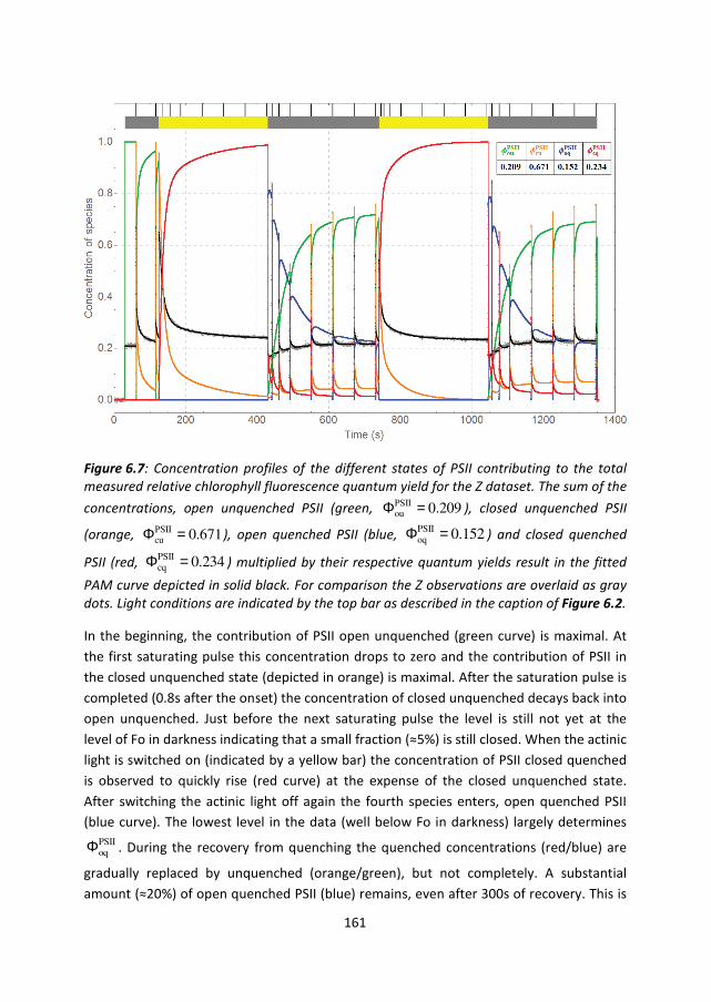
Figure 6.10: Simultaneous linked analysis of the Z and GA datasets. The Z data is shown in

orange dots, the fit in solid red and the residuals in dark gray. The GA data is plotted in

cyan dots, the fit in solid blue, and the residuals in light gray. All model parameters

between the two datasets are linked and shown in Table 6.1except for the rates of slow

and fast recovery (shown in the left table inset). The quantum yields estimated from the

linked analysis are shown in the right table inset.

Figure 6.10 shows the results of the linked analysis of the Z and GA datasets. Looking at

the fitted curves and the residuals in Figure 6.10 it is clear that a small price is paid by

linking all but one model parameter ( 8k , the rate of fast recovery), but overall both

datasets are described well with this single model with linked parameters. As more

parameters are unlinked (made free) the fit can improve. Looking at the values in Table

6.1 it can also be observed that the linked parameters resemble those estimated when

fitting the Z dataset alone. For instance the parameters for the fraction of slow quenching

( H1SQfr ) is estimated to be 0.27 for the Z dataset, 0.10 for the GA dataset, but 0.28 for the

Z+GA linked analysis. Thus the Z dataset contributes relatively more information in the

linked fit.

6.8 DISCUSSION

The key assumption made in this paper is that the fluorescence quantum yield as

measured by PAM fluorometry can be described by the sum of a number of discrete

molecular states, each with their own fluorescence quantum yield. This assumption

167

derives from the extensive study of photosynthetic samples using time-resolved

fluorescence spectroscopy where it can be shown that the observed fluorescence can also

be decomposed in the contributions by different complexes (Snellenburg et al. 2016)

facilitated by sophisticated target analysis (van Stokkum et al. 2004). We demonstrate

that the quantum yields estimated from the analysis of the PAM data are consistent with

the quantum yields estimated from ultra-fast time-resolved fluorescence spectroscopy

data, see Table S 6.4 in the Supporting Information section “The link with time-resolved

fluorescence spectroscopy”. Although PSI is part of our parametric model specification

and its quantum yield is also estimated in the time-resolved measurements, we have

chosen not to include it in the main text/figures for two reasons: (1) PSI contributes only a

constant offset as its quantum yield is not significantly affected by the actinic light

conditions, therefore it will not affect the estimated dynamics and (2) the results from our

analysis of time-resolved fluorescence show the contribution of PSI to be rather small, on

the order of 4% of Fm or 20% at Fo (given 475nm excitation, assuming 1:1 stoichiometry of

PSII:PSI). This justifies neglecting the contribution of PSI in first approximation if we’re

only interested in comparing the relative effect in PSII, but it does signify the importance

of a parametric model based analysis which can account for the influence of PSI when it is

needed, especially considering the effect on the estimated relative quantum yields. The

resulting decomposition including PSI is shown in Figure S 6.8 (concentrations) and Figure

S 6.9 (contributions).

Another strong assumption that we have made is that the number of species stays

constant throughout the measurement, especially with respect to the sample devoid of

zeaxanthin (V sample). In reality the chloroplasts in this sample might accumulate some

zeaxanthin throughout the measurement, which has recently been demonstrated to

function as a short-term light memory in plants (Matuszyńska et al. 2016). This would

imply that the population dynamics of PSII would have to be modelled with a total of eight

species (present in the inset table of Figure 6.9). This would be in agreement with the so

called four state two site quenching description of PSII (Matuszyńska et al. 2016;

Holzwarth et al. 2009), which attributes the fast induced quenching to a mechanism

driven by the pH sensing protein PsbS and the slower quenching to the formation of

zeaxanthin (Kiss et al. 2008; Li et al. 2004; Crouchman et al. 2006). However, despite our

simplification to only four states for PSII per measurement, we have demonstrated an

overall good agreement with the data. In order to facilitate the comparison between our

bottom-up approach and the top-down approach by Matuszyńska et al. we have used our

light protocol in their simulation code and generated a comparable decomposition (see

Figure S 6.12). In their model Matuszyńska et al. take into account a fraction of open and

closed PSII and a total level of quenching dependent on the relative concentrations of

PsBs and Zeaxanthin. This amounts to a gradually increasing level of quenching of all PSII

168

RC’s, rather than a gradual population switch between unquenched and quenched centers

as is the case in our model. The comparison between our V dataset and the prediction of

Figure S 6.12 shows that although there is reasonable qualitative agreement much of the

dynamics is not yet captured. The analysis of Figure 6.8 can inspire the iterative

improvement of the top-down theoretical model. In particular, a fraction closed

unquenched seems necessary.

Fluorescence quenching analysis by means of PAM fluorometry is a useful tool to study

NPQ in different samples under a wide variety of physiologically relevant conditions. In

one experiment the information about the condition of the sample before illumination,

during quenching inducing continuous actinic light and during recovery can be obtained

(Figure 6.2). Underlying the fluorescence quantum yield measured by the PAM

fluorometer are the contributions from a number of different emissive species,

summarized in Figure 6.1 for the case of plants. Each species corresponds to a pigment-

protein complex with its own concentration and its own absorption and emission

signature for the combination of excitation by the PAM instrument measuring light and its

detection window. This simple observation is enough to then formulate equation 1, which

states that the observed PAM signal can be parametrized as the sum of a number of

species’ concentrations multiplied by their quantum yields (Figure 1.6). Even for a typical

PAM analysis quenching experiment as depicted in Figure 6.2, the concentration function

can get complicated rather quickly, because the concentration of each species is not only

dependent on the light conditions at time t, but also on the light conditions at all times

prior to this. By segmenting the dataset based on changes in the light condition

experienced by the sample, either due to the presence or absence of measuring light or

the presence or absence of actinic light, and observing which segments preceded, it

becomes possible to describe the dynamics for each segment with a limited number of

functions (see Table S 6.1). In principle the segmentation can be entirely automated if the

PAM measurement protocol is known, although the start and end time point for each

segment can also be determined empirically from the data, either by manual inspection or

by fitting it. Each function is composed of a number of basis functions from a so called

Basis Function Set as detailed in the section “Components of a parametric model for the

PAM curves” in the SI on page 174. For this paper the aim was to keep the function

description as simple as possible, so all concentration dynamics is essentially described by

a number of exponential functions (for the rise and decay) and a constant term (to reflect

the transitional effects). For instance the closing of PSII RCs due to the application of a

saturating pulse is modelled by a single exponential rise (thus the concentration of open

PSII RCs, defined as one minus the concentration of closed PSII RCs is modeled by a single

exponential decay). From the inset of Figure 6.5 it can be seen that this is not a perfect

description of the observed rise, but it captures the trend and more importantly the

169

starting and end concentration are modelled correctly. It is known from the literature that

this fluorescence induction dynamics is much more complex than can be captured by a

single exponential rise, and many papers have been published that model this dynamics in

great detail (e.g. (Lazár 2003; Zhu et al. 2005) reviewed in (Stirbet and Govindjee 2012;

Kalaji et al. 2014). It was shown that when data is obtained at a higher time-resolution at

least 3 exponentials are needed (Vredenberg 2000; Joly and Carpentier 2009), in which

case it would be worthwhile to extend the Basis Function Set to capture this dynamics, but

for the datasets used in this work only 13 data points are observed during a saturating

pulse and a single exponential sufficed. Overall it can be seen from Figure 6.5 and

Figure 6.6 that with the limited set of functions described in Table S 6.1 the data can be

mimicked quite accurately. Of course with a full parameterized description of the PAM

curve it is also possible to gain more insight in the closing and quenching dynamics by

overlaying the data with the concentration profiles of the individual species as shown in

Figure 6.7; the sum of the products of the quantum yields (inset) and their concentrations

then reproduce the observed PAM fluorescence quantum yield (cf. equation 2). A

parameterized description allows for the use of standard non-linear regression to

estimate the parameters from the data as is demonstrated in Figure 6.9 for the V and Z

datasets. But the real power of a parametrized description is revealed when multiple

datasets are fitted simultaneously with a common set of parameters. The simplest

application of this is when instead of averaging several measurements on the same

sample, the measurements are analyzed with a single model resulting in statistically

relevant quantities with a meaningful standard deviation. This can be done even when

there is a small shift in the exact time of the saturating pulses or of the moment of

switching on the actinic light between measurements, which would significantly distort

the averaged data. A more advanced application is shown in Figure 6.10 where the Z and

the GA measurements, with at first sight completely different dynamics, are

simultaneously fitted with a common set of parameters and only a single free parameter

between the two datasets. In this way the hypothesis of what exactly happens to the

quenching dynamics upon the addition of glutaraldehyde can be more rigorously tested.

The fitted parameters obtained by fitting each dataset individually, as well as the

parameters obtained in the combined fit, are listed in Table 6.1 These results demonstrate

that the analysis of a single PAM fluorometry quenching experiment can already provide

information on the relative quantum yield of the four different states of PSII for the intact

chloroplasts. To the best of our knowledge no other form of spectroscopy provides this

information in a single measurement.

6.9 CONCLUSIONS

We have shown that it is feasible to formulate a parameterized description of PAM

fluorometry data, which decomposes the total observed fluorescence quantum yield into

170

the sum of the product of a number of distinct species and their quantum yields. We have

shown that the estimated quantum yields from PAM fluorometry data are largely

consistent with those estimated from target analysis of time-resolved fluorescence

spectroscopy. This creates a framework for developing a unifying model between two

different modes of spectroscopy that are ultimately measuring the same thing. Having an

explicit parameterization for PAM fluorometry data also does away with hand waving and

qualitative comparisons between measurements, all implicit and explicit assumption are

easily revealed by the model. Fitting a model directly to the data and extracting

statistically relevant parameters provides a framework to develop the true biophysical

model underlying the observations.

Acknowledgments This research is performed as part of the BioSolar Cells research

programme, sponsored by the Dutch Ministry of Economic Affairs. IHMvS and RvG

acknowledge financial support of the European Research Council (Advanced Grant

Proposal 267333 (PHOTPROT) to RvG). RvG gratefully acknowledges his Academy

Professor grant from the Netherlands Royal Academy of Sciences (KNAW). AVR

acknowledges the Leverhulme Trust grant RPG-2012-478 and UK Biotechnology and

Biological Sciences Research Council grant BB/L019027/1. AVR would like to acknowledge

The Royal Society for the Wolfson Research Merit Award. MPJ would like to acknowledge

the Leverhulme Trust grant ECF-2012-398\2. JM Gruber and LW Bielczynski are thanked

for helpful discussions regarding the interpretation of the modeling.

REFERENCES

Acuna AM, Snellenburg JJ, Gwizdala M, Kirilovsky D, van Grondelle R, van Stokkum IHM (2016) Resolving the contribution of the uncoupled phycobilisomes to cyanobacterial pulse-amplitude modulated (PAM) fluorometry signals. Photosynth Res 127 (1):91-102

Belgio E, Johnson MP, Jurić S, Ruban AV (2012) Higher plant photosystem II light-harvesting antenna, not the reaction center, determines the excited-state lifetime-both the maximum and the nonphotochemically quenched. Biophysical journal 102:2761-2771

Belyaeva N, Bulychev A, Riznichenko GY, Rubin A (2016) Thylakoid membrane model of the Chl a fluorescence transient and P700 induction kinetics in plant leaves. Photosynthesis Research:1-25

Bilger W, Schreiber U, Bock M (1995) Determination of the quantum efficiency of photosystem II and of non-photochemical quenching of chlorophyll fluorescence in the field. Oecologia 102:425-432

Crouchman S, Ruban A, Horton P (2006) PsbS enhances nonphotochemical fluorescence quenching in the absence of zeaxanthin. Febs Letters 580 (8):2053-2058

Ebenhöh O, Fucile G, Finazzi G, Rochaix J-D, Goldschmidt-Clermont M (2014) Short-term acclimation of the photosynthetic electron transfer chain to changing light: a

171

mathematical model. Philosophical Transactions of the Royal Society of London B: Biological Sciences 369 (1640):20130223

Ebenhöh O, Houwaart T, Lokstein H, Schlede S, Tirok K (2011) A minimal mathematical model of nonphotochemical quenching of chlorophyll fluorescence. Biosystems 103:196-204

Golub GH, Pereyra V (1973) The Differentiation of Pseudo-Inverses and Nonlinear Least Squares Problems Whose Variables Separate. SIAM Journal on Numerical Analysis 10 (2):413-432

Holzwarth AR, Jahns P (2014) Non-photochemical quenching mechanisms in intact organisms as derived from ultrafast-fluorescence kinetic studies. In: Non-Photochemical Quenching and Energy Dissipation in Plants, Algae and Cyanobacteria. Springer, pp 129-156

Holzwarth AR, Lenk D, Jahns P (2013) On the analysis of non-photochemical chlorophyll fluorescence quenching curves: I. Theoretical considerations. Biochim Biophys Acta 1827 (6):786-792

Holzwarth AR, Miloslavina Y, Nilkens M, Jahns P (2009) Identification of two quenching sites active in the regulation of photosynthetic light-harvesting studied by time-resolved fluorescence. Chemical Physics Letters 483 (4):262-267

Johnson MP, Pérez-Bueno ML, Zia A, Horton P, Ruban AV (2009) The zeaxanthin-independent and zeaxanthin-dependent qE components of nonphotochemical quenching involve common conformational changes within the photosystem II antenna in Arabidopsis. Plant physiology 149:1061-1075

Johnson MP, Ruban AV (2009) Photoprotective energy dissipation in higher plants involves alteration of the excited state energy of the emitting chlorophyll(s) in the light harvesting antenna II (LHCII). Journal of Biological Chemistry 284:23592-23601

Joly D, Carpentier R (2009) Sigmoidal reduction kinetics of the photosystem II acceptor side in intact photosynthetic materials during fluorescence induction. Photochemical & Photobiological Sciences 8 (2):167-173

Kalaji HM, Goltsev V, Brestic M, Bosa K, Allakhverdiev SI, Strasser RJ, Govindjee (2014) In Vivo Measurements of Light Emission in Plants.69-96

Kiss AZ, Ruban AV, Horton P (2008) The PsbS protein controls the organization of the photosystem II antenna in higher plant thylakoid membranes. J Biol Chem 283 (7):3972-3978

Lazár D (2003) Chlorophyll a fluorescence rise induced by high light illumination of dark-adapted plant tissue studied by means of a model of photosystem II and considering photosystem II heterogeneity. J Theor Biol 220 (4):469-503

Lazár D, Schansker G (2009) Models of Chlorophyll a Fluorescence Transients. Photosynthesis in Silico 29:85-123

Li X-P, Gilmore AM, Caffarri S, Bassi R, Golan T, Kramer D, Niyogi KK (2004) Regulation of photosynthetic light harvesting involves intrathylakoid lumen pH sensing by the PsbS protein. J Biol Chem 279 (22):22866-22874

Matuszyńska A, Ebenhöh O (2015) A reductionist approach to model photosynthetic self-regulation in eukaryotes in response to light. Biochem Soc Trans 43 (6):1133-1139

172

Matuszyńska A, Heidari S, Jahns P, Ebenhöh O (2016) A mathematical model of non-photochemical quenching to study short-term light memory in plants. Biochimica et Biophysica Acta (BBA) - Bioenergetics 1857 (12):1860-1869

Mullen KM, van Stokkum IHM (2007) TIMP: An R Package for Modeling Multi-Way Spectroscopic Measurements. Journal of Statistical Software 18 (3)

Peterson RB, Oja V, Eichelmann H, Bichele I, Dall’Osto L, Laisk A (2014) Fluorescence F 0 of photosystems II and I in developing C3 and C4 leaves, and implications on regulation of excitation balance. Photosynthesis research 122 (1):41-56

Pfündel EE, Klughammer C, Meister A, Cerovic ZG (2013) Deriving fluorometer-specific values of relative PSI fluorescence intensity from quenching of F0 fluorescence in leaves of Arabidopsis thaliana and Zea mays. Photosynthesis Research 114:189-206

Ritchie RJ (2008) Fitting light saturation curves measured using modulated fluorometry. Photosynthesis Research 96:201-215

Rubin A, Riznichenko G (2009) Modeling of the Primary Processes in a Photosynthetic Membrane. In: Laisk A, Nedbal L, Govindjee (eds) Photosynthesis in silico: Understanding Complexity from Molecules to Ecosystems. Springer, Netherlands, pp 151–176

Schansker G, Tóth SZ, Kovács L, Holzwarth AR, Garab G (2011) Evidence for a fluorescence yield change driven by a light-induced conformational change within photosystem II during the fast chlorophyll a fluorescence rise. Biochimica et Biophysica Acta (BBA)-Bioenergetics 1807 (9):1032-1043

Schansker G, Tóth SZ, Strasser RJ (2005) Methylviologen and dibromothymoquinone treatments of pea leaves reveal the role of photosystem I in the Chl a fluorescence rise OJIP. Biochimica et Biophysica Acta (BBA)-Bioenergetics 1706 (3):250-261

Schreiber U (2004) Pulse-amplitude modulation (PAM) fluorometry and saturation pulse method: an overview. In: Chlorophyll a fluorescence: a signature of photosynthesis. pp 279-319

Schreiber U, Schliwa U, Bilger W (1986) Continuous recording of photochemical and non-photochemical chlorophyll fluorescence quenching with a new type of modulation fluorometer. Photosynthesis Research 10:51-62

Snellenburg JJ, Dekker JP, van Grondelle R, van Stokkum IHM (2013) Functional compartmental modeling of the photosystems in the thylakoid membrane at 77 K. J Phys Chem B 117 (38):11363-11371

Snellenburg JJ, Laptenok SP, Seger R, Mullen KM, Stokkum IHMv (2012) Glotaran: A Java-Based Graphical User Interface for the R Package TIMP. Journal of Statistical Software 49 (3)

Snellenburg JJ, Wlodarczyk LM, Dekker JP, van Grondelle R, van Stokkum IH (2016) A model for the 77K excited state dynamics in Chlamydomonas reinhardtii in state 1 and state 2. Biochimica et Biophysica Acta (BBA)-Bioenergetics

Stirbet A, Govindjee (2012) Chlorophyll a fluorescence induction: A personal perspective of the thermal phase, the J-I-P rise. Photosynthesis Research 113:15-61

van Stokkum IHM, Larsen DS, van Grondelle R (2004) Global and target analysis of time-resolved spectra. Biochim Biophys Acta 1657 (2-3):82-104

173

van Stokkum IHM, van Oort B, van Mourik F, Gobets B, van Amerongen H (2008) (Sub)-picosecond spectral evolution of fluorescence studied with a synchroscan streak-camera system and target analysis. In: Biophysical techniques in photosynthesis. Springer, pp 223-240

Vredenberg WJ (2000) A three-state model for energy trapping and chlorophyll fluorescence in photosystem II incorporating radical pair recombination. Biophysical journal 79:26-38

Zaks J, Amarnath K, Kramer DM, Niyogi KK, Fleming GR (2012) A kinetic model of rapidly reversible nonphotochemical quenching. Proceedings of the National Academy of Sciences 109:15757-15762

Zhu XG, Govindjee, Baker NR, deSturler E, Ort DR, Long SP (2005) Chlorophyll a fluorescence induction kinetics in leaves predicted from a model describing each discrete step of excitation energy and electron transfer associated with photosystem II. Planta 223 (1):114-133

174

Supporting Information

Materials and Methods

The relevant sections of the material and methods section from (Johnson and Ruban

2009) are reproduced below with minor modifications and clarifications.

Chloroplasts Isolation—Spinach plants were grown for 8–9 weeks in Sanyo plant growth

cabinets with an 8-h photoperiod at a light intensity of 250 µmol of photons m-2s-1 and a

day/night temperature of 22/18 °C. Intact chloroplasts were prepared as described by

(Crouchman et al. 2006). Chloroplasts devoid of zeaxanthin and antheraxanthin (labeled -

Zea or just V) were prepared from spinach leaves dark adapted for 1 h. Chloroplasts

enriched in zeaxanthin (labeled +Zea or Z) were prepared from leaves pretreated for 30

min at 350 µmol of photons m-2s-1 under 98% N2, 2% O2.

PAM fluorometry—Chlorophyll fluorescence was measured with a Dual-PAM-100

chlorophyll fluorescence photosynthesis analyzer (Heinz Walz) using the liquid cell

adapter. Intact chloroplasts were measured in a quartz cuvette at a concentration of 12

μM chlorophyll under continuous stirring in the presence of 100μM methyl viologen as a

terminal electron acceptor. Actinic illumination (350 µmol of photons m-2s-1) was provided

by arrays of 635 nm LEDs. Fo (the fluorescence level with PSII reaction centers open) was

measured in the presence of a 10 µmol of photons m-2s-1 measuring beam (fluorescence

emitter: 620 nm (DUAL-DB)). The maximum fluorescence in the dark adapted state (Fm),

during the course of actinic illumination (Fm’) and in the subsequent dark relaxation

periods was determined using a 0.8 s saturating light pulse (4000 µmol of photons m-2s-1).

Time-resolved Fluorescence Spectroscopy—Time-correlated single photon counting

measurements were performed using a FluoTime 200 ps fluorometer (PicoQuant).

Fluorescence lifetime decay kinetics were measured on LHCII and intact chloroplasts (4

μM chlorophyll) using excitation provided by a 470-nm laser diode using a 10 MHz

repetition rate. These settings were carefully chosen to be far below the onset of singlet-

singlet exciton annihilation (<0.1 pJ). Time-resolved emission spectra (TRES) were

measured in the 655–760-nm detection region with 1-nm steps. The resolution of the

time-to-amplitude converter was 4 ps/channel.

Components of a parametric model for PAM curves

This section contains a detailed specification of the function required to fit the PAM

quenching analysis curves measured from intact chloroplasts as described in the previous

175

section. The fitting function takes into account the possible contributions to the observed

chlorophyll fluorescence quantum yield from the supercomplexes Photosystem II (PSII)

and Photosystem I (PSI) and (disconnected) Light Harvesting Complex II (LHCII). Here the

PSII contribution is assumed to be a linear superposition of four possible states, each with

a unique quantum yield, related to the state of the PSII RC (open or closed) and the rate of

non-photochemical quenching of the PSII supercomplex. Other contributions such as from

disconnected Chlorophyll molecules, different chromophores such as phycobilins (relevant

for the measured fluorescence in Cyanobacteria (Acuna et al. 2016)) or specific

experimentally related background contributions are not included in this specification, but

can be easily included if needed. Considering the large number of contributions to the

fitting function, it is important to keep the specification as concise as possible. A compact

way to list the contributions to the fitting function for a particular pigment-protein

complex is using the tensor product (also called outer product) of its independent state

vectors:

{ } { }, , {{ , },{ , }}o c u q ou oq cu cq⊗ = Eq.S1

The product cq then represents the function that describes the concentration of PSII in

the closed, quenched state. For the total contribution J to the PAM signal each

concentration function still needs to be multiplied with its quantum yield jklΦ , where the

additional indices k and l represent different light–acclimated states; in the case of PSII k

takes into account whether the state is open or closed and l stands for either a quenched

or an unquenched species. This can be achieved by taking the result of the tensor product,

flattening the 2 dimensional tensor in a column wise manner{ , , , }ou oq cu cq and then

taking the inner product with the respective yield parameters. This operations is

abbreviated using a helper function termed outer product function (OPF), with an

additional label to indicate which species it describes. For PSII this is written as:

{ } { } { } { } { }{ }PSII PSII PSII PSII PSII PSIIou oq cu cq

PSII PSII PSII PSIIou oq cu cq

J OPF , , , OPF , , , , , , ,o c u q o c u q

ou oq cu cq

= = Φ Φ Φ Φ = Φ + Φ + Φ + Φ

Eq.S2

And for LHCII, which only occurs in quenched or unquenched form, this is written as:

{ } { } { }{ }LHCII LHCII LHCII LHCIIu q

LHCII LHCIIu q

J OPF , OPF , , ,

,

u q u q

u q

= = Φ Φ = Φ Φ

Eq.S3

176

In the case of the contribution from PSI the most compact notation is simply the product

of concentration and quantum yield:

PSI PSIPSIJ c= Φ Eq.S4

Finally it is necessary to account for the stoichiometry between the contributions using

fractional parameters, e.g. for PSII, LHCII and PSI respectively LHCII(1 )fr− , LHCIIfr and

PSIfr . This is necessary to account for the relative stoichiometry of the proteins

themselves, but also to account for the relative difference in absorption at the excitation

wavelength used to excite the sample. In this way, when the contribution of PSI and

disconnected LHCII can be neglected the fractional constant is just 1. In the case that PSI

can be neglected but there is a fair amount of disconnected LHCII then the fraction also

sums up to 1.

In the follow paragraphs the exact equations used to construct the fitting function are

listed clustered per light regime (dark adapted sample, quenching inducing high light

following darkness, recovery in darkness following high light) and given a label so that

they can be referenced in subsequent function definitions using the notation

BFS["function_label"] , where BFS refers to “Basis Function Set” The equations are listed

in the order of the light conditions which they describe occur in the experiment described

in the main text (see section “Analyzing a full PAM quenching curve” and Figure 6.2)

Darkness (da)

In the region where there is only measuring light and no source of actinic light, the

Photosystem II (PSII) reaction centers (RCs) are assumed to be in the open state. If the

sample is also dark adapted (has not seen any strong source of actinic light for a long

enough period of time) it is also unquenched. Under these light conditions PSII has a

fluorescence quantum yield PSIIouΦ . However at the same time it is possible to have

contributions to the total signal of unconnected Light Harvesting Complex II (LHCII) and

Photosystem I (PSI). This can then be summarized in the equation for a dark adapter

(“da”) segment:

PSII LHCII PSILHCII ou LHCII PSI"da" (1 ) ufr fr fr→ − Φ + Φ + Φ Eq.S5

The next change in light conditions is a saturation pulse applied at time 0t , with the

continuous actinic light source still switched off. To describe the sudden rise in measured

fluorescence quantum yield, due to the closing of PSII RC’s, a mono exponential function is

used “dkspIRF” with rate constant 1k . The subsequent recovery toward the level where all

177

PSII RC’s are again open is modeled using three exponential decays (rate constants k2, k3,

k3b).

L1 0( )

e"dkspIRF"k t t− −→ ,

L2 0( )

e"dkspD1"k t t− −→ ,

L3 0( )

e"dkspD2"k t t− −→ ,

L3b 0( )

"dk " espD2bk t t− −→

Eq.S6

Here L represents a label to distinguish the parameters for the same function used in

different light conditions. The same functional description can then be used to describe

the effect of a specific change in light conditions (e.g. a saturating pulse in darkness) but

observed differences in kinetics can then be taken into account by freeing some

parameters. The data described in the main manuscript required freeing the rate k3

between the first two saturating pulses in darkness for a dark acclimated sample, and the

remaining saturating pulses in darkness for a sample that had already been exposed to

high light. Then for the first two saturation pulses in darkness k3 is then defined as SP13k

and for the rest the parameter D13k is used. The rates D1 D1

2 3, bk k are the same (linked)

throughout.

A careful reader might notice that the fluorescence induction dynamics and subsequent

relaxation is captured using just a few exponentials, implying underlying first order

differential equations. This is a strong assumption but not a necessary one. If more

information is available on the dynamics of a particular transition this a priori knowledge

can be used to refine the components of the fit function.

With the above definitions the rise of the fluorescence in darkness can be written as:

( ) [ ][ ]

PSIIouPSIIcu LHCII PSI

LHCII LHCII u PSI

,,

"dkspR" 1 OPFBFS "dkspIRF" ,

1 BFS "dkspIRF"

fr fr fr

Φ Φ → − + Φ + Φ −

Eq.S7

The subsequent decay is then described as:

178

[ ]( )( )( ) [ ]( )

( ) [ ]( )[ ]

( ) ( ) [ ]( ) [ ]( )

L2

L L3b 2

L L3b 2

L2

L L3b 2

L L3b

PSIIouPSIIcu

LHCII

2

1 BFS "dkspD1"

1 1 1 BFS "dkspD2" ,

"dkspD"1 * 1 BFS "dkspD2b"

* "dkspD1"

1 * 1 *BFS "dkspD

,,

(1 )O

2"

* 1 * B

PF

FS "dkspD2b"

fr

fr fr

fr fr

fr BFS

fr fr

fr fr

fr

− + − − − + → − − +

− −

Φ Φ

−

+

−LHCII PSI

LHCII u PSIfr fr

+ Φ + Φ

Eq.S8

Where the fractional parameters L L2 3b,fr fr are introduced to express the amplitudes of

the exponential decays of Eq.S6. For the first two periods of darkness these parameters

are defined as 12 bD1 D

3,fr fr , expect for the first saturating pulse which uses SP S2 3

1 P1b,fr fr .

Darkness to high light (dk2hl)

When a period of (high) continuous actinic light follows a period of darkness a number of

additional function definitions are needed. First the function “dkendC” evaluates the

function “dkspD” for the time point just before the dark to light transition tLR1end and

quantifies the amount of closed PSII left over due to only partial recovery from a

saturating pulse in darkness.

[ ] LR1end"dkendC" BFS "dkspD" with t t→ → Eq.S9

The fluorescence induction dynamics due to the continuous actinic light is again described

using a single exponential, but with a different rate constant.

( )10 0e"dkhlIRF"Lk t t− −→ Eq.S10

Assuming that upon switching to continuous light all the PSII RC’s are closed, a small

fraction (depending on the absolute level of light intensity) of the RC’s can again re-open if

the excitation pressure is not enough to keep them completely closed, which is accounted

for using a single exponential, where a certain fraction ( )H1CC1 fr− of the PSII RCs reopens.

The amount of closed PSII can then be described as

179

( ) 6 ( )H1 H1CC CC"hlPSIIc" 1 e LLRk t t

fr fr− −→ − + Eq.S11

where tLLR is substituted with the timepoint of the last light regime (thus (t- tLLR) is the time

since switching on the actinic light). The amount of open PSII RCs is simply one minus the

closed concentration.

[ ]"hlPSIIo" 1 BFS "hlPSIIc"→ − Eq.S12

Using these function definitions the amount of PSII closed/open in the dark to high light

transition can be written as

[ ][ ]( ) [ ] [ ]( )

"dk2hlPSIIc" BFS "dkendC"

1 BFS "dkendC" BFS "hlPSIIc" 1 BFS "dkhlIRF"

→ +− −

"dk2hlPSIIo" 1 - BFS["dk2hlPSIIc"]→

Eq.S13

During a period of high light non-photochemical quenching is induced, leading to a lower

observed fluorescence quantum yield. This is captured in a quenching function which

describes the decay of the unquenched population.

To account for a small fraction of initially quenched PSII we define two functions. A

fraction isqfr which can be left over from a previous partial recovery, and a fraction ifqfr

due to very fast quenching unresolvable given the limited time-resolution of the

experiment (60ms time steps in this case).

L Lisq ifq"ISQ" ,"IFQ"fr fr→ → Eq.S14

Out of the total amount that can be quenched H1Qfr a certain fraction is associated with a

relatively slow recovery and therefore indicated with the label “SQ”: H1SQfr , described by a

single exponential. Another fraction recovers relatively quickly “FQ”: H1SQ1 fr− , and can be

fitted as the sum of 2 exponentials.

[ ]( ) ( )H14 1

SQ"hlUnQS" 1 BFS "ISQ" ea LRk t t

fr −− −→ −

Eq.S15

180

[ ]( ) ( ) ( ) ( )1 14 51 11 1

4 4"hlUnQF" 1 BFS "IFQ" e 1 eH H

LR LRk t t k t tH Hfr fr− −− − − − → − + −

The total function for the relative amount of unquenched and quenched concentration is

then written as:

( ) [ ] ( ) [ ]( )Q Q SQ SQ"hlUnQ" 1 * BFS "hlUnQS" 1 BFS "hlUnQF"fr fr fr fr→ − + + −

[ ]"hlQ" 1 BFS "hlUnQ"→ −

Eq.S16

The full expression to describe the darkness to high light transition can now be assembled:

( ) [ ]( ) [ ]{ }[ ] [ ]{ }

[ ] [ ]{ }{ }

PSIILHCII

LHCII PSILHCII PSI

BFS "dk2hlPSIIo" ,BFS "dk2hlPSIIc" ,"dk2hl" 1 OPF

BFS "hlQ" ,BFS "hlUnQ"

OPF BFS "hlQ" , BFS "hlUnQ"

fr

fr fr

→ − +

+ Φ

Eq.S17

During the period of continuous actinic light, there are also periodically saturating pulses

given to ensure that all PSII RCs are fully closed. The necessary function to fit this aspect in

the data is similar to the saturating pulses applied during darkness expect that the kinetics

is much faster and both the rise and decay can be fitted with a single exponential.

11 0( )

"hlspIRF" eH

k t t− −→ ,1

2 0( )"hlspD1" e

Hk t t− −→ Eq.S18

This then leads to the amount of open/closed PSII during a saturating pulse

during high light being described by:

[ ] [ ]( )"hlspPSIIo" BFS "hlspIRF" 1 BFS "hlPSIIc"→ −

[ ] [ ]( ) [ ]( )"hlspPSIIc" BFS "hlPSIIc" 1 BFS "hlspIRF" 1 BFS "hlPSIIc"→ + − −

Eq.S19

When the above function definitions are combined the expression for the rise and decay

of fluorescence yield during actinic light can respectively be written as:

181

( ) [ ]( ) [ ]{ }[ ] [ ]{ }

[ ] [ ]{ }{ }

PSIILHCII

LHCII PSILHCII PSI

BFS "hlspPSIIo" ,BFS "hlspPSIIc" ,"hlspR" 1 OPF

BFS "hlQ" ,BFS "hlUnQ"

OPF BFS "hlQ" , BFS "hlUnQ"

fr

fr fr

→ − +

+ Φ

Eq.S20

( )

[ ]( ) [ ]( )[ ]( ) [ ]

[ ][ ] [ ]{ }

[ ] [ ]{ }{ }

PSIILHCII

LHCII PSLHCII PSI

1 BFS "hlspD1" BFS "hlPSIIo" ,

1 BFS "hlPSIIc" BFS "hlspD1" ,"hlspD" 1 OPF

BFS "hlPSIIc"

BFS "hlQ" , BFS "hlUnQ"

OPF BFS "hlQ" , BFS "hlUnQ"

fr

fr fr

− − + → − +

+ Φ I

Eq.S21

High light to darkness or recovery (hl2dk)

In a period of darkness, following actinic light, the induced non-photochemical quenching

gradually recovers. The starting point for the recovery can be determined by evaluating

the quenching function at the end of the high light period, just before the recovery period.

[ ]( )1 1 2LR LR LR"SQT" 1 BFS "hlUnQS" with t t t t

− − −→ − − → −

[ ]( )1 1 2LR LR LR"FQT" 1 BFS "hlUnQF" with t t t t

− − −→ − − → −

Eq.S22

The dynamics of recovery consists of two parts both fitted with a single exponential. One

part of the induced quenching is recovered from very slowly ( H1SQfr ) given by rate k8a,

while the other part recovers quickly ( )H1SQ1 fr− given by rate k8.

( )R18 LR 1"hldkRecF" 1 e

k t t −− −→ − ,

( )R18a LR 1"hldkRecS" 1 e

k t t −− −−→ ,

( )( )H1 H1 H1Q SQ SQ"hldkRec" BFS["hldkRecS"]) + BFS["hldkRecF"]1fr fr fr→ −

,

Eq.S23

While recovery from NPQ is a relatively slow process, the reopening of PSII RCs is quite

fast and results in a quick transition from mostly open PSII RCs in actinic light, to

completely open RCs in the recovery phase. The dynamics of this transition is captured by

the same function which describes reopening after a saturating pulse.

182

[ ]( )( )( ) [ ]( )

( ) [ ]( )

L2

L L3b 2

L L3b 2

"hl2dkPSIIo" 1 BFS "dkspD1"

1 1 1 BFS "dkspD2"

1 * 1 BFS "dkspD2b"

fr

fr fr

fr fr

→ − +

− − − +

− −

,

[ ]( ) ( ) [ ]

( ) [ ]( )

L2

L L3b 2

L L3b 2

"hl2dkPSIIc" "dkspD1"

1 1 BFS "dkspD2"

1 * BFS "dkspD2b"

fr BFS

fr fr

fr fr

→ +− − +

−

,

Eq.S24

With L L2 3b,fr fr equal to 1

2 bD1 D

3,fr fr during the first recovery period and 22 bR2 R

3,fr fr during

the second recovery period.

Finally the amount of unquenched and quenched PSII can then be expressed as:

[ ]( ) [ ] [ ]( )"hl2dkPSIIuS" 1 BFS "SQT" BFS "SQT" BFS "hldkRecS"→ − + ,

[ ]( ) [ ] [ ]( )"hl2dkPSIIuF" 1 BFS "FQT" BFS "FQT" BFS "hldkRecF"→ − + ,

( ) [ ] [ ]( )Q SQ SQ"hl2dkPSIIu" 1 BFS "hl2dkPSIIuF" BFS "hl2dkPSIIuS"fr fr fr→ − +,

[ ]"hl2dkPSIIq" 1 BFS "hl2dkPSIIu"→ −,

Eq.S25

The function definition that describes the quenching of LHCII can be postulated in the

same way, but is not specified here in detail as there is no data in the main text to test it

against. In a first approximation the quenching dynamics can be assumed to be the same

as for the LHCII-PSII complex. When these functions are combined the function that

described the transition from darkness to high light can be written as:

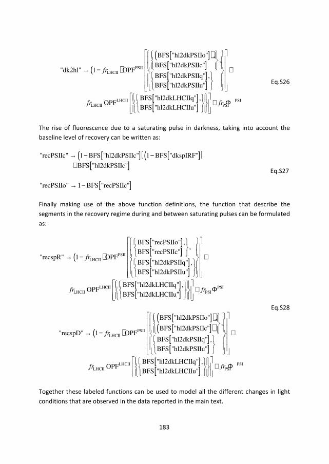
183

( )

[ ]( )[ ][ ][ ]

[ ][ ]

PSIILHCII

LHCIILHCII

BFS "hl2dkPSIIo" ,,

BFS "hl2dkPSIIc""dk2hl" 1 OPF

BFS "hl2dkPSIIq" ,

BFS "hl2dkPSIIu"

BFS "hl2dkLHCIIq" ,OPF

BFS "hl2dkLHCIIu"

fr

fr

→ − +

PSIPSIfr

+ Φ

Eq.S26

The rise of fluorescence due to a saturating pulse in darkness, taking into account the

baseline level of recovery can be written as:

[ ]( ) [ ]( )[ ]

"recPSIIc" 1 BFS "hl2dkPSIIc" 1 BFS "dkspIRF"

BFS "hl2dkPSIIc"

→ − −+

[ ]"recPSIIo" 1 BFS "recPSIIc"→ −

Eq.S27

Finally making use of the above function definitions, the function that describe the

segments in the recovery regime during and between saturating pulses can be formulated

as:

( )

[ ][ ][ ][ ]

[ ][ ]

PSIILHCII

LHCIILHCII

BFS "recPSIIo" ,,

BFS "recPSIIc""recspR" 1 OPF

BFS "hl2dkPSIIq" ,

BFS "hl2dkPSIIu"

BFS "hl2dkLHCIIq" ,OPF

BFS "hl2dkLHCIIu"

fr

fr fr

→ − +

+

PSIPSIΦ

( )

[ ]( )[ ]( )

[ ][ ]

[ ][ ]

PSIILHCII

LHCIILHCII

BFS "hl2dkPSIIo" ,,

BFS "hl2dkPSIIc""recspD" 1 OPF

BFS "hl2dkPSIIq" ,

BFS "hl2dkPSIIu"

BFS "hl2dkLHCIIq" ,OPF

BFS "hl2dkLHCIIu"

fr

fr

→ − +

PSIPSIfr

+ Φ

Eq.S28

Together these labeled functions can be used to model all the different changes in light

conditions that are observed in the data reported in the main text.

184

Working model for the sample devoid of zeaxanthin (V)

Figure S 6.1. Working mathematical model which ties the different species listed in

Figure 6.1 to the parametric description given in equation 2 for the sample devoid of

zeaxanthin (V). The premise of the model are four distinct states which can be

interconverted into one another with certain rates, either light driven (red arrows) or

spontaneously in the absence of light (blue arrows). The difference with the model for the

Z case is an additional rate k6 which represents re-opening of the reaction centers due to

insufficient actinic light pressure to keep them completely closed. A simplification of the

model is the assumption that the sample remains devoid of zeaxanthin over the course of

the measurement.

185

Segments Label Description Parameters introduced

1,26 “bg” Background signal, measuring light (ML) OFF

3 “da” Signal from a dark adapted sample (ML ON)

PSIIouΦ ;

LHCIILHCII , ufr Φ ; PSI

PSI ,fr Φ

4,6 “dkspR” Saturating pulse rise in darkness PSIIcuΦ , D1

1k

5,7,86 “dkspD” Saturating pulse decay in darkness D1 D1 D1 D1 D12 3b2 3 3b , ,, , fr frk k k , optionally SP1 SP1

2 3bSP13, ,kfr fr

9 “dk2hl” (1) Darkness to (high) actinic light H1 H1 H1 H1 H1 H1 H1Q SQ 4 4

PSII PSII D1oq 5cq 10 CC 6, , , , , ,, , ,fr fr fr k k fr kkΦ Φ ;

LHCIIqΦ

10,12,…,22 “hlspR” (1) Saturating pulse rise in actinic light H11k

11,13,…,23 “hlspD” (1) Saturating pulse decay in actinic light H12k

246,25 “hl2dk” (1) Actinic light to darkness transition R1 R18 8a,k k , optionally R1 R1

2 3b,fr fr

26,28,…,38 “recspR” (1) Saturating pulse rise in darkness during recovery

27,29,…39,406 “recspD” (1) Saturating pulse decay in darkness during recovery

41 “dk2hl” (2) Darkness to (high) actinic light (after recovery)

optionally 2 2 24 4 5, ,H H Hfr k k and 2

6Hk

42,44,…58 “hlspR” (2) Saturating pulse rise in actinic light (after recovery)

43,45,…59 “hlspD” (2) Saturating pulse decay in actinic light (after recovery)

6 These segments consist of only a single data point, between the end of one light regime and the start of the next. To describe this one transition point, the function of the previous or the next light regime is reused. This is a mechanism to deal with non-instantaneous light switching, although for the data reported in this simulation the switching occurred within the 60 ms time steps of the data.

186

606,61 “hl2dk” (2) 2nd Actinic light to darkness transition optionally R2 R22 3b,fr fr

62,64,…,74 “recspR” (2) Saturating pulse rise in darkness during 2nd recovery

63,65,…,75,766 “recspD” (2) Saturating pulse decay in darkness during 2nd recovery

77 “bg” Background signal after turning ML OFF. Table S 6.1: Full parameter table for the total fitting function for the 77 segments of the data. For each label a closed form expression is

available in the present section. Labels (1) and (2) signify the first and second time a particular expression is used, for which the

estimated parameters can have different numerical values. All parameters introduced for a function in a particular segment can be

optionally made free in repeated occurrences of that function for subsequent segments. Specifically some parameters are listed here

explicitly because they were freed in fitting one of the datasets described in the main text.

For SP1 ( )( ) ( )SP1 SP1 SP1 SP1 SP12 2 3 3b 2 3 3b 2, 1- 1- , 1-=ba fr a fr fr a fr fr= =

For SP2 ( )( ) ( )D1 D1 D1 D1 D12 2 3 3b 2 3 3b 2, 1- 1 =- , 1-ba fr a fr fr a fr fr= =

Table S 6.2. Relation between amplitude parameters used in the main text and fractions given in Table S 6.1.

Caption for Figure S 6.2: Annotated screenshot of the simulation of the Z data in Wolfram Mathematica 10. The simulation function is

underlined in red and takes as arguments: element out of a list of timepoints (r_timesZ) and arguments for which the controls are shown

to the right of the graphics. Note that the variables named differ slightly from those in the main text (most notablyH1 H14a SQk4aH1 k k= = ),

and not all variables are directly relevant for the simulation shown (for instance none of the parameters related to simulating

photodamage or different OJIP dynamics are used).

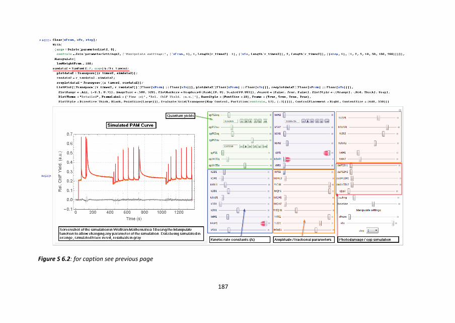
187

Figure S 6.2: for caption see previous page

188

Figure S 6.3. Level of NPQ (defined as: Fm/Fm’ -1) during a fluorescence quenching analysis experiment on intact Chloroplasts devoid of

zeaxanthin (black, labeled ‘V’) or enriched in zeaxanthin (red (‘Z’), blue (‘GA’)). The blue curve represents a sample where glutaraldehyde

(GA) was added (at t≈410s) to prevent the recovery from the quenched state. The level of NPQ is calculated directly from the fitting

function with the kinetic parameters that describe the decay following a saturating pulse set to zero (i.e. continuously in Fm’). In the

background the original data from Figure 6.2 of the main text is shown: the V dataset in gray, the Z dataset in orange and the GA

dataset in cyan. Light conditions indicated by the top bar as described in the caption of that figure.

189

Figure S 6.4: Concentration profiles of the different states of PSII contributing to the total measured relative chlorophyll fluorescence

quantum yield for the GA dataset. The sum of the concentrations, open unquenched PSII (green, PSIIou 0.207Φ = ), closed unquenched PSII

(orange, PS IIcu 0.701Φ = ), open quenched PSII (blue,

PSIIcq 0.159Φ = ) and closed quenched PSII (red,

PSIIcq 0.231Φ = ) multiplied by their

respective quantum yields produce the PAM curve depicted in solid black. For comparison the GA observations are overlaid as gray dots.

Light conditions indicated by the top bar as described in the caption of Figure 6.2.

190

Figure S 6.5. Contributions of the different states of PSII to the total measured relative chlorophyll fluorescence quantum yield for the Z

dataset. The contribution of a PSII state is defined as the product of its concentrations (shown in Figure 6.7) and the relative quantum

yields: open unquenched PSII (green, PSIIou 0.209Φ = ), closed unquenched PSII (orange, PS II

cu 0.671Φ = ), open quenched PSII (blue,

PSIIoq 0.152Φ = ) and closed quenched PSII (red,

PSIIcq 0.234Φ = ). The total fitted contribution is in solid black, observations depicted as

gray dots. Light conditions indicated by the top bar as described in the caption of Figure 6.2.

191

Figure S 6.6 Contributions of the different states of PSII to the total measured relative chlorophyll fluorescence quantum yield for the V

dataset. The contribution of a PSII state is defined as the product of its concentrations (shown in Figure 6.8) and the relative quantum

yields: open unquenched PSII (green, PSIIou 0.205Φ = ), closed unquenched PSII (orange, PSII

cu 1Φ = ), open quenched PSII (blue,

PSIIoq 0.185Φ = ) and closed quenched PSII (red,

PSIIcq 0.409Φ = ). The total fitted contribution is in solid black, observations depicted as

gray dots. Light conditions indicated by the top bar as described in the caption of Figure 6.2.

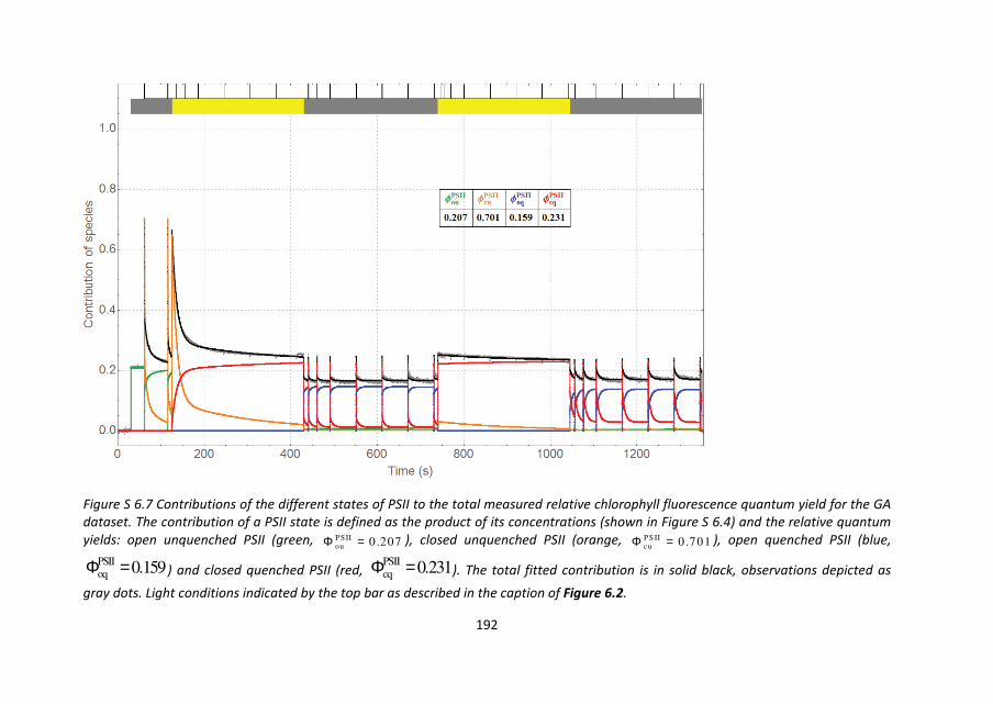
192

Figure S 6.7 Contributions of the different states of PSII to the total measured relative chlorophyll fluorescence quantum yield for the GA

dataset. The contribution of a PSII state is defined as the product of its concentrations (shown in Figure S 6.4) and the relative quantum

yields: open unquenched PSII (green, PSIIou 0.207Φ = ), closed unquenched PSII (orange, PS II

cu 0.701Φ = ), open quenched PSII (blue,

PSIIoq 0.159Φ = ) and closed quenched PSII (red,

PSIIcq 0.231Φ = ). The total fitted contribution is in solid black, observations depicted as

gray dots. Light conditions indicated by the top bar as described in the caption of Figure 6.2.

193

Figure S 6.8. Concentration profiles of the different states of PSII and PSI contributing to the total measured relative chlorophyll

fluorescence quantum yield for the V dataset. The sum of the concentrations, open unquenched PSII (green, PSIIou 0.16Φ = ), closed

unquenched PSII (orange, PSIIcu 0.93Φ = ), open quenched PSII (blue,

PSIIoq 0.12Φ = ), closed quenched PSII (red,

PSIIcq 0.37Φ = ) and PSI (cyan,

PSI 0.05Φ = ) multiplied by their respective quantum yields produce the PAM curve depicted in solid black. For comparison the V

observations are overlaid as gray dots. Light conditions indicated by the top bar as described in the caption of Figure 6.2.

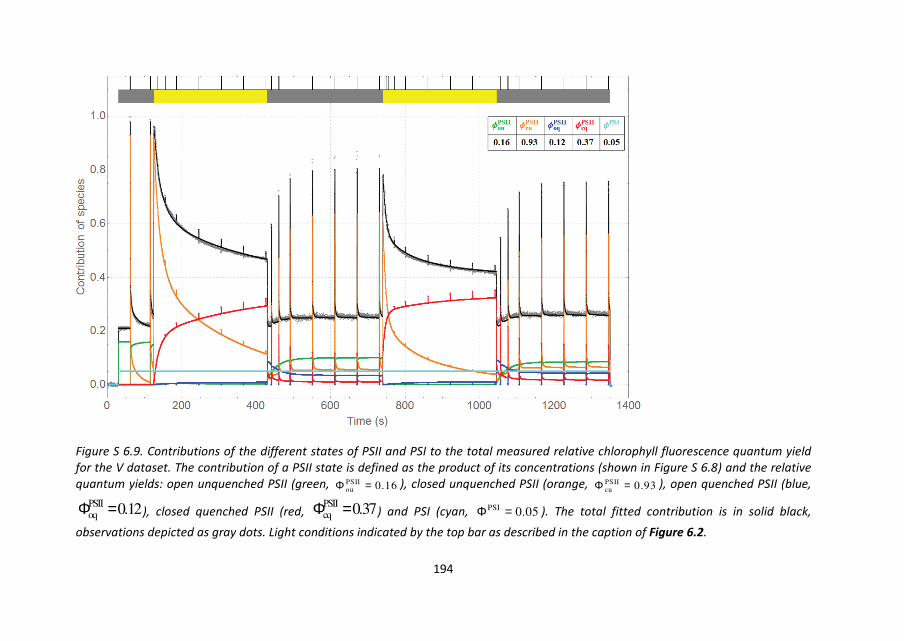
194

Figure S 6.9. Contributions of the different states of PSII and PSI to the total measured relative chlorophyll fluorescence quantum yield

for the V dataset. The contribution of a PSII state is defined as the product of its concentrations (shown in Figure S 6.8) and the relative

quantum yields: open unquenched PSII (green, PSIIou 0.16Φ = ), closed unquenched PSII (orange, PSII

cu 0.93Φ = ), open quenched PSII (blue,

PSIIoq 0.12Φ = ), closed quenched PSII (red,

PSIIcq 0.37Φ = ) and PSI (cyan, PSI 0.05Φ = ). The total fitted contribution is in solid black,

observations depicted as gray dots. Light conditions indicated by the top bar as described in the caption of Figure 6.2.

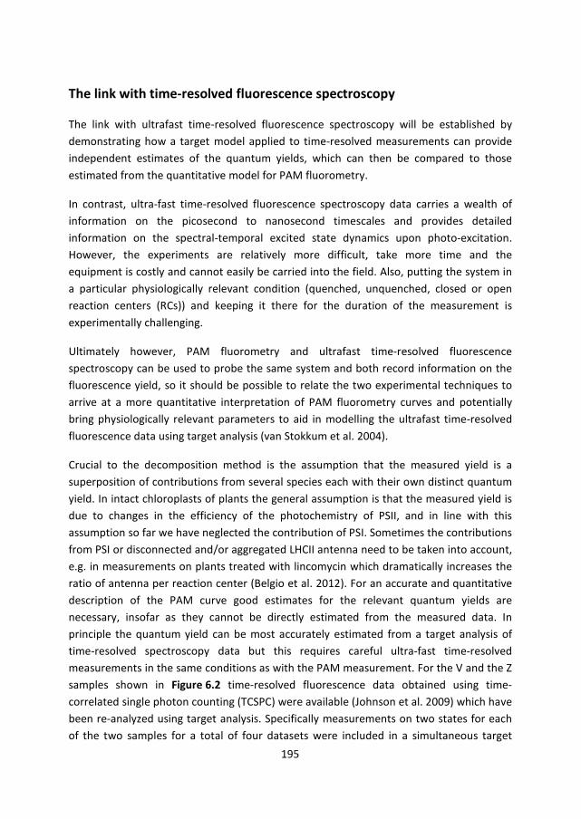
195

The link with time-resolved fluorescence spectroscopy

The link with ultrafast time-resolved fluorescence spectroscopy will be established by

demonstrating how a target model applied to time-resolved measurements can provide

independent estimates of the quantum yields, which can then be compared to those

estimated from the quantitative model for PAM fluorometry.

In contrast, ultra-fast time-resolved fluorescence spectroscopy data carries a wealth of

information on the picosecond to nanosecond timescales and provides detailed

information on the spectral-temporal excited state dynamics upon photo-excitation.

However, the experiments are relatively more difficult, take more time and the

equipment is costly and cannot easily be carried into the field. Also, putting the system in

a particular physiologically relevant condition (quenched, unquenched, closed or open

reaction centers (RCs)) and keeping it there for the duration of the measurement is

experimentally challenging.

Ultimately however, PAM fluorometry and ultrafast time-resolved fluorescence

spectroscopy can be used to probe the same system and both record information on the

fluorescence yield, so it should be possible to relate the two experimental techniques to

arrive at a more quantitative interpretation of PAM fluorometry curves and potentially

bring physiologically relevant parameters to aid in modelling the ultrafast time-resolved

fluorescence data using target analysis (van Stokkum et al. 2004).

Crucial to the decomposition method is the assumption that the measured yield is a

superposition of contributions from several species each with their own distinct quantum

yield. In intact chloroplasts of plants the general assumption is that the measured yield is

due to changes in the efficiency of the photochemistry of PSII, and in line with this

assumption so far we have neglected the contribution of PSI. Sometimes the contributions

from PSI or disconnected and/or aggregated LHCII antenna need to be taken into account,

e.g. in measurements on plants treated with lincomycin which dramatically increases the

ratio of antenna per reaction center (Belgio et al. 2012). For an accurate and quantitative

description of the PAM curve good estimates for the relevant quantum yields are

necessary, insofar as they cannot be directly estimated from the measured data. In

principle the quantum yield can be most accurately estimated from a target analysis of

time-resolved spectroscopy data but this requires careful ultra-fast time-resolved

measurements in the same conditions as with the PAM measurement. For the V and the Z

samples shown in Figure 6.2 time-resolved fluorescence data obtained using time-

correlated single photon counting (TCSPC) were available (Johnson et al. 2009) which have

been re-analyzed using target analysis. Specifically measurements on two states for each

of the two samples for a total of four datasets were included in a simultaneous target

196

analysis: closed unquenched (‘Fm’) and closed quenched (‘NPQ’) for the sample devoid of

Zeaxanthin (VFm, VNPQ) and for the sample enriched in Zeaxanthin (ZFm, ZNPQ) (see also

Figure 6.1). The state of the PSII RCs in the four datasets is assumed to be completely

closed for all datasets and either unquenched or fully quenched. Excitation occurred at

470 nm, predominantly exciting Chl b and Carotenoid, and thus relatively more PSII than

PSI.

The datasets were first globally analyzed individually, i.e. each dataset represented by a

matrix ( , )t λΨ was fitted to the minimal number ncomp of exponential decays convolved

with an instrument response function (IRF) required to satisfactorily fit the data up to the

noiseξ . For each wavelength the amplitude parameters of all exponential decays are

determined using the method of variable projection (Golub and Pereyra 1973) as

implemented by the free software TIMP (Mullen and van Stokkum 2007) and Glotaran

(Snellenburg et al. 2012). This results in a decay associated spectrum (DAS) for each

component. This can be summarized as:

( )( ) ( )comp( , ) exp[ ] IRF DAS ( , )n

l llt k t t tλ λ ξ λ Ψ = − ⊗ + ∑ Eq.S29

where lk is the rate of decay of each component, the reciprocal of which represents the

lifetime corresponding to that decay. For each measurement the IRF was independently

measured by scattered laser light. Each IRF was characterized by means of a primary

Gaussian shaped band, and a number of extra Gaussians shaped bands related to the

primary band by a certain scaling factor, a shift in time and a different width. In this way

the non-Gaussian nature of the IRF of the TCSPC detector could be very well

approximated while maintaining the advantages that a purely analytical model function

provides (van Stokkum et al. 2004) in contrast to numerically convolving the measured IRF

with the exponential decays. When fitting the data, all instrument response parameters

were fixed except for the position of the primary Gaussian band which was a free

parameter of the fit. This is almost always necessary because the IRF is typically measured

at a different wavelength than where the data is measured so there might be a small shift

due to dispersion and experimental variation might induce an additional shift. The

estimated lifetimes and their Decay Associated Spectra (DAS)are depicted in Figure S 6.10.

Six components were needed to describe each dataset up to the noise level. The fastest

lifetime is shorter than can reliably be estimated given the IRF width (≈110 ps FWHM) but

is necessary to account for a bit of relaxation from slightly more blue to redder Chl’s in the

first tens of ps of the experiment due to a selective excitation of Chl b. The first lifetime

that can reliably be resolved is around 0.07-0.1 ns and has a broad emission band peaking

around 710 nm, which can safely be attributed to PSI emission. In the ZNPQ datasets this

component is likely capturing a small fraction of fast quenching. The next three lifetimes

197

all feature a very similar spectral shape with emission around 680 nm reflecting emission

from the LHCII-PSII supercomplex. Clearly quenching is playing a major role on these

timescales, differently affecting the samples. The last lifetime represents a tiny fraction of

very long lived emission which is observed as a result of measuring for 50 ns. This

component likely represents some recombination fluorescence which can safely be

ignored. On the basis of one fast component emitting around 710 nm (black DAS) and

three DAS with similar shapes (red, blue and magenta) emitting around 680 nm a target

model can be constructed consisting of a PSI compartment in parallel to a LHCII-PSII

contribution.

Figure S 6.10: Global analysis results of the SPC measurements. For the two samples, V and

Z as described earlier, two conditions analog to the PAM measurement were probed:

closed unquenched (‘Fm’) and closed quenched (‘NPQ’). Shown are the decay associated

spectra (DAS) with the estimated lifetimes in the legends. Spectra are normalized to the

maximum of the first DAS, except in the case of ZFm where the 4th DAS had the largest

amplitude.

6.10 TARGET ANALYSIS RESULT

From the global analysis results it is not possible to directly obtain the quantum yield

parameters that can be related to the PAM fluorometry data, but it serves as a starting

198

point for a more detailed target analysis which takes into account the different

contributions originating from LHCII-PSII and PSI and the different levels of quenching.

To account for the observation of three lifetimes with a similar spectral shape a LHCII-PSII

compartment is placed in equilibrium with two (dark) radical pair states, i.e. assuming

reversible charge separation, see Figure S 6.11A. The LHCII-PSII compartment is assumed

to be fully equilibrated within the duration of the IRF. The only difference in the model

between the four datasets was the quenching rate Q from LHCII-PSII (shown in Figure S

6.11B) and the shape of the Species Associated Spectra (SAS, c.f. Figure S 6.11D). ). The

spectral freedom was needed because the SAS of the LHCII-PSII compartment in the V

datasets was less peaked than in the Z datasets irrespective of the Fm or NPQ condition.

No evidence was found for an additional quenching site, e.g. in the form of detached LHCII

as recently reviewed in (Holzwarth and Jahns 2014).

Figure S 6.11: Overview of simultaneous target analysis results on the four datasets. (A)

Target model for time-resolved emission from Chloroplasts at RT excited at 470 nm. All

rates (in 1/ns) are fitted parameters with 10% standard error. The input percentages are

estimated from an equal SAS area constraint (Snellenburg et al. 2013). (B) The quenching

rate indicated by Q in the target model for the four different datasets. (C) The population

profiles of the different components of the target model. The time axis is linear from -0.5

to 0.5 ns and logarithmic thereafter. (D) The SAS corresponding to the target model for the

V datasets (solid) and the Z datasets, with the spectra linked between the Fm and the NPQ

state for both. The shading reflects the spectral area used to calculate the relative

fluorescence quantum yield as observed by a PAM fluorometer.

Note that whereas in the V samples the quenching rate Q increases from 0.2 in Fm to only

0.48/ns in the NPQ condition, in the ZFm case it is already 0.43/ns. This rate then

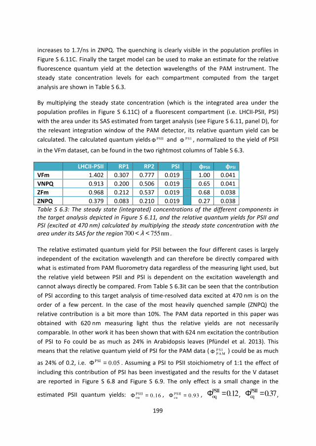
199

increases to 1.7/ns in ZNPQ. The quenching is clearly visible in the population profiles in

Figure S 6.11C. Finally the target model can be used to make an estimate for the relative

fluorescence quantum yield at the detection wavelengths of the PAM instrument. The

steady state concentration levels for each compartment computed from the target

analysis are shown in Table S 6.3.

By multiplying the steady state concentration (which is the integrated area under the

population profiles in Figure S 6.11C) of a fluorescent compartment (i.e. LHCII-PSII, PSI)

with the area under its SAS estimated from target analysis (see Figure S 6.11, panel D), for

the relevant integration window of the PAM detector, its relative quantum yield can be

calculated. The calculated quantum yields PSIIΦ and P S IΦ , normalized to the yield of PSII

in the VFm dataset, can be found in the two rightmost columns of Table S 6.3.

LHCII-PSII RP1 RP2 PSI φPSII φPSI

VFm 1.402 0.307 0.777 0.019 1.00 0.041

VNPQ 0.913 0.200 0.506 0.019 0.65 0.041

ZFm 0.968 0.212 0.537 0.019 0.68 0.038

ZNPQ 0.379 0.083 0.210 0.019 0.27 0.038 Table S 6.3: The steady state (integrated) concentrations of the different components in

the target analysis depicted in Figure S 6.11, and the relative quantum yields for PSII and

PSI (excited at 470 nm) calculated by multiplying the steady state concentration with the

area under its SAS for the region 700 755nmλ< < .

The relative estimated quantum yield for PSII between the four different cases is largely

independent of the excitation wavelength and can therefore be directly compared with

what is estimated from PAM fluorometry data regardless of the measuring light used, but

the relative yield between PSII and PSI is dependent on the excitation wavelength and

cannot always directly be compared. From Table S 6.3it can be seen that the contribution

of PSI according to this target analysis of time-resolved data excited at 470 nm is on the

order of a few percent. In the case of the most heavily quenched sample (ZNPQ) the

relative contribution is a bit more than 10%. The PAM data reported in this paper was

obtained with 620 nm measuring light thus the relative yields are not necessarily

comparable. In other work it has been shown that with 624 nm excitation the contribution

of PSI to Fo could be as much as 24% in Arabidopsis leaves (Pfündel et al. 2013). This

means that the relative quantum yield of PSI for the PAM data ( P S IP A MΦ ) could be as much

as 24% of 0.2, i.e. PSI 0.05Φ = . Assuming a PSI to PSII stoichiometry of 1:1 the effect of

including this contribution of PSI has been investigated and the results for the V dataset

are reported in Figure S 6.8 and Figure S 6.9. The only effect is a small change in the

estimated PSII quantum yields: PSIIou 0.16Φ = , PSII

cu 0.93Φ = , PSIIoq 0.12Φ = ,

PSIIcq 0.37Φ = ,

200

PSI 0.05Φ = . Because PSI contributes only an offset (no closing or quenching dynamics)

the data could still be fitted equally well.

At this point it makes sense to compare the quantum yields estimated from PAM

fluorometry as shown in Figure 6.9, Figure 6.10, and Table 6.1 with those estimated from

the target analysis of time-resolved fluorescence as shown in Figure S 6.11 and

summarized in Table S 6.3. The quantum yields that could be estimated from both

techniques are shown in Table S 6.4.

Dataset QY label rel. yield. SPC rel. yield. PAM

‘VFm’ PSII,VcuΦ 1.00 1.00

‘VNPQ’ PSII,VcqΦ 0.65 0.41

‘ZFm’ PSII,ZcuΦ 0.68 0.67

‘ZNPQ’ PSII,ZcqΦ 0.27 0.23

Table S 6.4: The relative quantum yields for the different states of PSII as could be

estimated from SPC data or PAM data.

The quantum yields estimated via either technique are relative to the quantum yield

obtained in the Fm case of the V sample. In the case of the PAM fluorometry

measurements this is done by normalizing the data to the maximal level of fluorescence in

darkness (Fm) where it can be assumed that the only contribution is PSII closed

unquenched. In the case of the time-resolved measurement the integrated contribution of

LHCII-PSII in the VFm dataset is defined to be 1, the LHCII-PSII contributions in the other

datasets are related to this. In the time-resolved data the quantum yield is corrected for

the PSI contribution, meaning a small relative error between the two methods is to be

expected. Despite this there is considerable consistency in the estimated quantum yields,

except perhaps for the VNPQ case. However it should be noted here that the limited time-

resolution of the TCSPC setup (≈110 ps FWHM) meant that it was not possible to reliably

quantify quenching processes faster than this, meaning that in the SPC measurement the

quantum yield can easily be overestimated due to underestimating the amount of NPQ

taking place at early timescales, whereas the yield estimated from the PAM is a reflection

of the true quantum yield. This discrepancy could be further investigated by obtaining

time-resolved measurements with a much higher time-resolution, for instance using a

streak camera setup (van Stokkum et al. 2008). Also from the results of the analysis of the

PAM curve for the V dataset presented in Figure 6.9 it can be seen that making sure that

the excitation pressure is high enough to keep all RC continuously closed is challenging.

The VNPQ case could reflect a mixture of open/closed as well as quenched/unquenched.

201

6.11 SIMULATIONS USING THE MATUSZYNSKA ET AL. 2016 MODEL

Thanks to the availability of the complete simulation source code of the model

(Matuszyńska et al. 2016) it was possible to adapt our own light protocol and use it as

input for their model. Note that the model was calibrated for the simulation of PAM

fluorometry on Arabidopsis leafs and not spinach chloroplast, which might explain some

inaccuracies in the prediction. Following the same open source philosophy the source

code to reproduce these figures is provided in a supplemental file included with this SI.

Below follows a brief description in words.

Read in our own raw data (plain csv file) and extract the column with the V fluorescence

trace.

Read in our own light protocol stored as two separate files (json format), one containing

the timing information on the saturating pulses and the other containing information

about the light regimes. Convert this light protocol to the format required by the model.

Initialize the model (type: ‘Arabidopsis’) with the default parameters and initialize the

simulation.

Integrate the model over the times provided by the light protocol.

Extract the PSII state variables (open: B0; closed B2) and the degree of quenching Q(t),

required for the plotting.

The simulated fluorescence quantum yield Φ can now be described as the sum of the

quantum yield in PSII state 0 (open)0stΦ and PSII in state 2 (closed)

2stΦ :

0 F F H PQ 0

2 F F H 2

0 2 0 2

(t) = k / (k + k * Q(t) + k ) * B (t)

(t) = k / (k + k * Q(t)) * B (t)

(t) ( (t) (t)) / max( )

st

st

st st st st

ΦΦΦ = Φ + Φ Φ + Φ

Eq.S30

where Fk is the rate of intrinsic fluorescence decay, kH is the rate of quenching

(dissipated as heat) and kPQ is the rate of photochemistry. The rate of NPQ is given by

kH*Q(t), which is modulated by the quencher activity Q which is in turn dependent on the

relative concentration of PsbS [PsbS] and Zeaxanthin [Zx], defined as:

0 1

2 3

(1 )[PsbS] (1 )[PsbS ]

[PsbS ] [PsbS]

Ps s

Ps s

Q Z Z

Z Z

γ γγ γ

= − + −+ +

Eq.S31

where [ ]

[ ]s

ZSat

ZxZ

Zx k=

+ reflects the contribution of Zx to the quenching and kZSat is a half-

saturation constant. The γ parameters were fitted by (Matuszyńska et al. 2016).

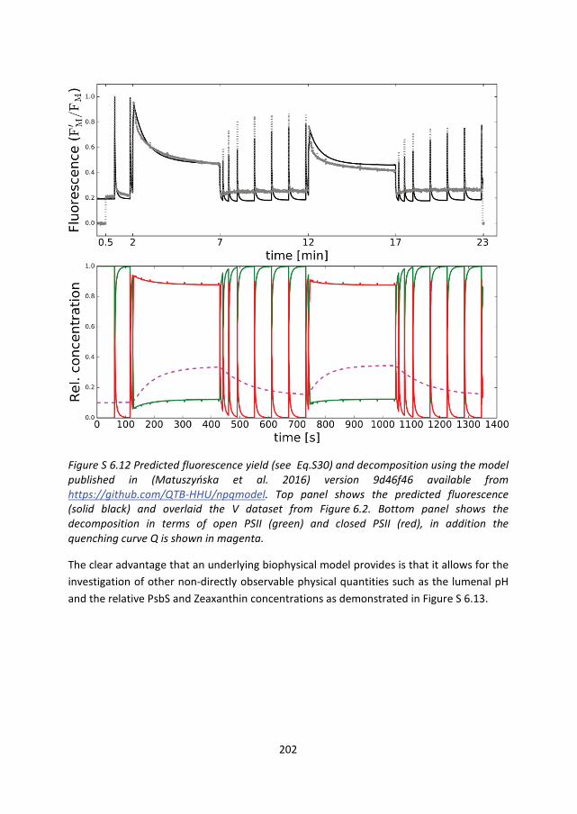
202

Figure S 6.12 Predicted fluorescence yield (see Eq.S30) and decomposition using the model

published in (Matuszyńska et al. 2016) version 9d46f46 available from

https://github.com/QTB-HHU/npqmodel. Top panel shows the predicted fluorescence

(solid black) and overlaid the V dataset from Figure 6.2. Bottom panel shows the

decomposition in terms of open PSII (green) and closed PSII (red), in addition the

quenching curve Q is shown in magenta.

The clear advantage that an underlying biophysical model provides is that it allows for the

investigation of other non-directly observable physical quantities such as the lumenal pH

and the relative PsbS and Zeaxanthin concentrations as demonstrated in Figure S 6.13.

203

Figure S 6.13. In analogy to Figure 5 from (Matuszyńska et al. 2016), (top panel) the

visualization of lumenal pH changes in the response to our light protocol. (middle panel)

the dynamics of the quenching components (solid line for the relative zeaxanthin

concentration, dashed line for the ratio of protonated PsbS), (bottom panel) The phase

plane trajectories of the quenching variable (Q) and the lumenal pH during our light

protocol.