Embed Size (px)
Citation preview

EUROPEAN PHARMACOPOEIA 6.0 5.3. Statistical analysis
01/2008:50300
5.3. STATISTICAL ANALYSISOF RESULTS OF BIOLOGICALASSAYS AND TESTS
1. INTRODUCTIONThis chapter provides guidance for the design of bioassaysprescribed in the European Pharmacopoeia (Ph. Eur.)and for analysis of their results. It is intended for use bythose whose primary training and responsibilities are notin statistics, but who have responsibility for analysis orinterpretation of the results of these assays, often withoutthe help and advice of a statistician. The methods ofcalculation described in this annex are not mandatory forthe bioassays which themselves constitute a mandatory partof the Ph. Eur. Alternative methods can be used and maybe accepted by the competent authorities, provided thatthey are supported by relevant data and justified during theassay validation process. A wide range of computer softwareis available and may be useful depending on the facilitiesavailable to, and the expertise of, the analyst.Professional advice should be obtained in situations where :a comprehensive treatment of design and analysis suitablefor research or development of new products is required ; therestrictions imposed on the assay design by this chapter arenot satisfied, for example particular laboratory constraintsmay require customized assay designs, or equal numbersof equally spaced doses may not be suitable ; analysis isrequired for extended non-linear dose-response curves,for example as may be encountered in immunoassays. Anoutline of extended dose-response curve analysis for onewidely used model is nevertheless included in Section 3.4and a simple example is given in Section 5.4.
1.1. GENERAL DESIGN AND PRECISIONBiological methods are described for the assay of certainsubstances and preparations whose potency cannot beadequately assured by chemical or physical analysis. Theprinciple applied wherever possible throughout these assaysis that of comparison with a standard preparation so asto determine how much of the substance to be examinedproduces the same biological effect as a given quantity, theUnit, of the standard preparation. It is an essential conditionof such methods of biological assay that the tests on thestandard preparation and on the substance to be examined becarried out at the same time and under identical conditions.For certain assays (determination of virus titre for example)the potency of the test sample is not expressed relative to astandard. This type of assay is dealt with in Section 4.5.Any estimate of potency derived from a biological assayis subject to random error due to the inherent variabilityof biological responses and calculations of error should bemade, if possible, from the results of each assay, even whenthe official method of assay is used. Methods for the designof assays and the calculation of their errors are, therefore,described below. In every case, before a statistical methodis adopted, a preliminary test is to be carried out with anappropriate number of assays, in order to ascertain theapplicability of this method.The confidence interval for the potency gives an indication ofthe precision with which the potency has been estimated inthe assay. It is calculated with due regard to the experimentaldesign and the sample size. The 95 per cent confidence
interval is usually chosen in biological assays. Mathematicalstatistical methods are used to calculate these limits so as towarrant the statement that there is a 95 per cent probabilitythat these limits include the true potency. Whether thisprecision is acceptable to the European Pharmacopoeiadepends on the requirements set in the monograph for thepreparation concerned.The terms “mean” and “standard deviation” are used here asdefined in most current textbooks of biometry.The terms “stated potency” or “labelled potency”, “assignedpotency”, “assumed potency”, “potency ratio” and “estimatedpotency” are used in this section to indicate the followingconcepts :— “stated potency” or “labelled potency” : in the case of
a formulated product a nominal value assigned fromknowledge of the potency of the bulk material ; in thecase of bulk material the potency estimated by themanufacturer ;
— “assigned potency” : the potency of the standardpreparation ;
— “assumed potency” : the provisionally assigned potencyof a preparation to be examined which forms the basis ofcalculating the doses that would be equipotent with thedoses to be used of the standard preparation ;
— “potency ratio” of an unknown preparation ; the ratio ofequipotent doses of the standard preparation and theunknown preparation under the conditions of the assay ;
— “estimated potency” : the potency calculated from assaydata.
Section 9 (Glossary of symbols) is a tabulation of the moreimportant uses of symbols throughout this annex. Wherethe text refers to a symbol not shown in this section or usesa symbol to denote a different concept, this is defined in thatpart of the text.
2. RANDOMISATION ANDINDEPENDENCE OF INDIVIDUALTREATMENTSThe allocation of the different treatments to differentexperimental units (animals, tubes, etc.) should be madeby some strictly random process. Any other choice ofexperimental conditions that is not deliberately allowed forin the experimental design should also be made randomly.Examples are the choice of positions for cages in a laboratoryand the order in which treatments are administered. Inparticular, a group of animals receiving the same dose ofany preparation should not be treated together (at thesame time or in the same position) unless there is strongevidence that the relevant source of variation (for example,between times, or between positions) is negligible. Randomallocations may be obtained from computers by using thebuilt-in randomisation function. The analyst must checkwhether a different series of numbers is produced every timethe function is started.The preparations allocated to each experimental unit shouldbe as independent as possible. Within each experimentalgroup, the dilutions allocated to each treatment are notnormally divisions of the same dose, but should be preparedindividually. Without this precaution, the variabilityinherent in the preparation will not be fully representedin the experimental error variance. The result will be anunder-estimation of the residual error leading to:1) an unjustified increase in the stringency of the test for theanalysis of variance (see Sections 3.2.3 and 3.2.4),
General Notices (1) apply to all monographs and other texts 571

5.3. Statistical analysis EUROPEAN PHARMACOPOEIA 6.0
2) an under-estimation of the true confidence limits for thetest, which, as shown in Section 3.2.5, are calculated fromthe estimate of s2, the residual error mean square.
3. ASSAYS DEPENDING UPONQUANTITATIVE RESPONSES
3.1. STATISTICAL MODELS
3.1.1. GENERAL PRINCIPLESThe bioassays included in the Ph. Eur. have been conceivedas “dilution assays”, which means that the unknownpreparation to be assayed is supposed to contain the sameactive principle as the standard preparation, but in a differentratio of active and inert components. In such a case theunknown preparation may in theory be derived from thestandard preparation by dilution with inert components. Tocheck whether any particular assay may be regarded as adilution assay, it is necessary to compare the dose-responserelationships of the standard and unknown preparations. Ifthese dose-response relationships differ significantly, thenthe theoretical dilution assay model is not valid. Significantdifferences in the dose-response relationships for thestandard and unknown preparations may suggest that one ofthe preparations contains, in addition to the active principle,other components which are not inert but which influencethe measured responses.
To make the effect of dilution in the theoretical modelapparent, it is useful to transform the dose-responserelationship to a linear function on the widest possible rangeof doses. 2 statistical models are of interest as models forthe bioassays prescribed : the parallel-line model and theslope-ratio model.
The application of either is dependent on the fulfilment ofthe following conditions :
1) the different treatments have been randomly assigned tothe experimental units,
2) the responses to each treatment are normally distributed,
3) the standard deviations of the responses within eachtreatment group of both standard and unknown preparationsdo not differ significantly from one another.
When an assay is being developed for use, the analyst has todetermine that the data collected from many assays meetthese theoretical conditions.
— Condition 1 can be fulfilled by an efficient use of Section 2.
— Condition 2 is an assumption which in practice is almostalways fulfilled. Minor deviations from this assumptionwill in general not introduce serious flaws in the analysisas long as several replicates per treatment are included.In case of doubt, a test for deviations from normality (e.g.the Shapiro-Wilk(1) test) may be performed.
— Condition 3 can be checked with a test for homogeneityof variances (e.g. Bartlett’s(2) test, Cochran’s(3) test).Inspection of graphical representations of the data canalso be very instructive for this purpose (see examplesin Section 5).
When conditions 2 and/or 3 are not met, a transformationof the responses may bring a better fulfilment of theseconditions. Examples are ln y, , y2.
— Logarithmic transformation of the responses y to ln ycan be useful when the homogeneity of variances is notsatisfactory. It can also improve the normality if thedistribution is skewed to the right.
— The transformation of y to is useful when theobservations follow a Poisson distribution i.e. when theyare obtained by counting.
— The square transformation of y to y2 can be useful if, forexample, the dose is more likely to be proportional tothe area of an inhibition zone rather than the measureddiameter of that zone.
For some assays depending on quantitative responses,such as immunoassays or cell-based in vitro assays, a largenumber of doses is used. These doses give responses thatcompletely span the possible response range and produce anextended non-linear dose-response curve. Such curves aretypical for all bioassays, but for many assays the use of a largenumber of doses is not ethical (for example, in vivo assays)or practical, and the aims of the assay may be achievedwith a limited number of doses. It is therefore customary torestrict doses to that part of the dose-response range which islinear under suitable transformation, so that the methods ofSections 3.2 or 3.3 apply. However, in some cases analysis ofextended dose-response curves may be desirable. An outlineof one model which may be used for such analysis is given inSection 3.4 and a simple example is shown in Section 5.4.
There is another category of assays in which the responsecannot be measured in each experimental unit, but in whichonly the fraction of units responding to each treatment canbe counted. This category is dealt with in Section 4.
3.1.2. ROUTINE ASSAYSWhen an assay is in routine use, it is seldom possible to checksystematically for conditions 1 to 3, because the limitednumber of observations per assay is likely to influence thesensitivity of the statistical tests. Fortunately, statisticianshave shown that, in symmetrical balanced assays, smalldeviations from homogeneity of variance and normality donot seriously affect the assay results. The applicability ofthe statistical model needs to be questioned only if a seriesof assays shows doubtful validity. It may then be necessaryto perform a new series of preliminary investigations asdiscussed in Section 3.1.1.
2 other necessary conditions depend on the statistical modelto be used :
— for the parallel-line model :
4A) the relationship between the logarithm of the doseand the response can be represented by a straight lineover the range of doses used,
5A) for any unknown preparation in the assay the straightline is parallel to that for the standard.
— for the slope-ratio model :
4B) the relationship between the dose and the responsecan be represented by a straight line for each preparationin the assay over the range of doses used,
5B) for any unknown preparation in the assay the straightline intersects the y-axis (at zero dose) at the same pointas the straight line of the standard preparation (i.e. theresponse functions of all preparations in the assay musthave the same intercept as the response function of thestandard).
(1) Wilk, M.B. and Shapiro, S.S. (1968). The joint assessment of normality of several independent samples, Technometrics 10, 825-839.(2) Bartlett, M.S. (1937). Properties of sufficiency and statistical tests, Proc. Roy. Soc. London, Series A 160, 280-282.(3) Cochran, W.G. (1951). Testing a linear relation among variances, Biometrics 7, 17-32.
572 See the information section on general monographs (cover pages)
EUROPEAN PHARMACOPOEIA 6.0 5.3. Statistical analysis
Conditions 4A and 4B can be verified only in assays in whichat least 3 dilutions of each preparation have been tested. Theuse of an assay with only 1 or 2 dilutions may be justifiedwhen experience has shown that linearity and parallelism orequal intercept are regularly fulfilled.
After having collected the results of an assay, and beforecalculating the relative potency of each test sample, ananalysis of variance is performed, in order to check whetherconditions 4A and 5A (or 4B and 5B) are fulfilled. Forthis, the total sum of squares is subdivided into a certainnumber of sum of squares corresponding to each conditionwhich has to be fulfilled. The remaining sum of squaresrepresents the residual experimental error to which theabsence or existence of the relevant sources of variation canbe compared by a series of F-ratios.
When validity is established, the potency of each unknownrelative to the standard may be calculated and expressed asa potency ratio or converted to some unit relevant to thepreparation under test e.g. an International Unit. Confidencelimits may also be estimated from each set of assay data.
Assays based on the parallel-line model are discussed inSection 3.2 and those based on the slope-ratio model inSection 3.3.
If any of the 5 conditions (1, 2, 3, 4A, 5A or 1, 2, 3, 4B,5B) are not fulfilled, the methods of calculation describedhere are invalid and an investigation of the assay techniqueshould be made.
The analyst should not adopt another transformationunless it is shown that non-fulfilment of the requirementsis not incidental but is due to a systematic change in theexperimental conditions. In this case, testing as described inSection 3.1.1 should be repeated before a new transformationis adopted for the routine assays.
Excess numbers of invalid assays due to non-parallelismor non-linearity, in a routine assay carried out to comparesimilar materials, are likely to reflect assay designs withinadequate replication. This inadequacy commonly resultsfrom incomplete recognition of all sources of variabilityaffecting the assay, which can result in underestimation ofthe residual error leading to large F-ratios.
It is not always feasible to take account of all possiblesources of variation within one single assay (e.g. day-to-dayvariation). In such a case, the confidence intervals fromrepeated assays on the same sample may not satisfactorilyoverlap, and care should be exercised in the interpretationof the individual confidence intervals. In order to obtaina more reliable estimate of the confidence interval it maybe necessary to perform several independent assays andto combine these into one single potency estimate andconfidence interval (see Section 6).
For the purpose of quality control of routine assays it isrecommended to keep record of the estimates of the slopeof regression and of the estimate of the residual error incontrol charts.
— An exceptionally high residual error may indicate sometechnical problem. This should be investigated and,if it can be made evident that something went wrongduring the assay procedure, the assay should be repeated.An unusually high residual error may also indicatethe presence of an occasional outlying or aberrantobservation. A response that is questionable because offailure to comply with the procedure during the courseof an assay is rejected. If an aberrant value is discoveredafter the responses have been recorded, but can then betraced to assay irregularities, omission may be justified.The arbitrary rejection or retention of an apparently
aberrant response can be a serious source of bias. Ingeneral, the rejection of observations solely because atest for outliers is significant, is discouraged.
— An exceptionally low residual error may once in a whileoccur and cause the F-ratios to exceed the critical values.In such a case it may be justified to replace the residualerror estimated from the individual assay, by an averageresidual error based on historical data recorded in thecontrol charts.
3.1.3. CALCULATIONS AND RESTRICTIONSAccording to general principles of good design the following3 restrictions are normally imposed on the assay design.They have advantages both for ease of computation and forprecision.a) Each preparation in the assay must be tested with thesame number of dilutions.b) In the parallel-line model, the ratio of adjacent doses mustbe constant for all treatments in the assay ; in the slope-ratiomodel, the interval between adjacent doses must be constantfor all treatments in the assay.c) There must be an equal number of experimental units toeach treatment.If a design is used which meets these restrictions, thecalculations are simple. The formulae are given inSections 3.2 and 3.3. It is recommended to use softwarewhich has been developed for this special purpose. Thereare several programs in existence which can easily dealwith all assay-designs described in the monographs. Not allprograms may use the same formulae and algorithms, butthey should all lead to the same results.Assay designs not meeting the above mentioned restrictionsmay be both possible and correct, but the necessaryformulae are too complicated to describe in this text. A briefdescription of methods for calculation is given in Section 7.1.These methods can also be used for the restricted designs, inwhich case they are equivalent with the simple formulae.The formulae for the restricted designs given in this textmay be used, for example, to create ad hoc programs ina spreadsheet. The examples in Section 5 can be used toclarify the statistics and to check whether such a programgives correct results.
3.2. THE PARALLEL-LINE MODEL
3.2.1. INTRODUCTIONThe parallel-line model is illustrated in Figure 3.2.1.-I. Thelogarithm of the doses are represented on the horizontal axiswith the lowest concentration on the left and the highestconcentration on the right. The responses are indicated onthe vertical axis. The individual responses to each treatmentare indicated with black dots. The 2 lines are the calculatedln(dose)-response relationship for the standard and theunknown.Note : the natural logarithm (ln or loge) is used throughoutthis text. Wherever the term “antilogarithm” is used, thequantity ex is meant. However, the Briggs or “common”logarithm (log or log10) can equally well be used. In this casethe corresponding antilogarithm is 10x.For a satisfactory assay the assumed potency of the testsample must be close to the true potency. On the basisof this assumed potency and the assigned potency of thestandard, equipotent dilutions (if feasible) are prepared, i.e.corresponding doses of standard and unknown are expectedto give the same response. If no information on the assumedpotency is available, preliminary assays are carried out overa wide range of doses to determine the range where thecurve is linear.
General Notices (1) apply to all monographs and other texts 573

5.3. Statistical analysis EUROPEAN PHARMACOPOEIA 6.0
Figure 3.2.1.-I. – The parallel-line model for a 3 + 3 assayThe more nearly correct the assumed potency of theunknown, the closer the 2 lines will be together, for theyshould give equal responses at equal doses. The horizontaldistance between the lines represents the “true” potency ofthe unknown, relative to its assumed potency. The greaterthe distance between the 2 lines, the poorer the assumedpotency of the unknown. If the line of the unknown issituated to the right of the standard, the assumed potencywas overestimated, and the calculations will indicatean estimated potency lower than the assumed potency.Similarly, if the line of the unknown is situated to the left ofthe standard, the assumed potency was underestimated, andthe calculations will indicate an estimated potency higherthan the assumed potency.
3.2.2. ASSAY DESIGNThe following considerations will be useful in optimising theprecision of the assay design :1) the ratio between the slope and the residual error shouldbe as large as possible,2) the range of doses should be as large as possible,3) the lines should be as close together as possible, i.e. theassumed potency should be a good estimate of the truepotency.The allocation of experimental units (animals, tubes, etc.) todifferent treatments may be made in various ways.
3.2.2.1. Completely randomised designIf the totality of experimental units appears to be reasonablyhomogeneous with no indication that variability in responsewill be smaller within certain recognisable sub-groups, theallocation of the units to the different treatments should bemade randomly.If units in sub-groups such as physical positions orexperimental days are likely to be more homogeneous thanthe totality of the units, the precision of the assay maybe increased by introducing one or more restrictions intothe design. A careful distribution of the units over theserestrictions permits irrelevant sources of variation to beeliminated.
3.2.2.2. Randomised block designIn this design it is possible to segregate an identifiable sourceof variation, such as the sensitivity variation between littersof experimental animals or the variation between Petri dishesin a diffusion microbiological assay. The design requiresthat every treatment be applied an equal number of times in
every block (litter or Petri dish) and is suitable only when theblock is large enough to accommodate all treatments once.This is illustrated in Section 5.1.3. It is also possible to use arandomised design with repetitions. The treatments shouldbe allocated randomly within each block. An algorithm toobtain random permutations is given in Section 8.5.
3.2.2.3. Latin square designThis design is appropriate when the response may beaffected by two different sources of variation each of whichcan assume k different levels or positions. For example, in aplate assay of an antibiotic the treatments may be arrangedin a k × k array on a large plate, each treatment occurringonce in each row and each column. The design is suitablewhen the number of rows, the number of columns and thenumber of treatments are equal. Responses are recorded ina square format known as a Latin square. Variations due todifferences in response among the k rows and among thek columns may be segregated, thus reducing the error. Anexample of a Latin square design is given in Section 5.1.2.An algorithm to obtain Latin squares is given in Section 8.6.More complex designs in which one or more treatments arereplicated within the Latin square may be useful in somecircumstances. The simplified formulae given in this Chapterare not appropriate for such designs, and professional adviceshould be obtained.
3.2.2.4. Cross-over designThis design is useful when the experiment can be sub-dividedinto blocks but it is possible to apply only 2 treatments toeach block. For example, a block may be a single unit thatcan be tested on 2 occasions. The design is intended toincrease precision by eliminating the effects of differencesbetween units while balancing the effect of any differencebetween general levels of response at the 2 occasions. If2 doses of a standard and of an unknown preparation aretested, this is known as a twin cross-over test.
The experiment is divided into 2 parts separated by a suitabletime interval. Units are divided into 4 groups and each groupreceives 1 of the 4 treatments in the first part of the test.Units that received one preparation in the first part of thetest receive the other preparation on the second occasion,and units receiving small doses in one part of the test receivelarge doses in the other. The arrangement of doses is shownin Table 3.2.2.-I. An example can be found in Section 5.1.5.
Table 3.2.2.-I. — Arrangement of doses in cross-over design
Group of units Time I Time II
1 S1 T2
2 S2 T1
3 T1 S2
4 T2 S1
3.2.3. ANALYSIS OF VARIANCEThis section gives formulae that are required to carry out theanalysis of variance and will be more easily understood byreference to the worked examples in Section 5.1. Referenceshould also be made to the glossary of symbols (Section 9).
The formulae are appropriate for symmetrical assays whereone or more preparations to be examined (T, U, etc.) arecompared with a standard preparation (S). It is stressedthat the formulae can only be used if the doses are equallyspaced, if equal numbers of treatments per preparation areapplied, and each treatment is applied an equal number oftimes. It should not be attempted to use the formulae in anyother situation.
574 See the information section on general monographs (cover pages)

EUROPEAN PHARMACOPOEIA 6.0 5.3. Statistical analysis
Apart from some adjustments to the error term, the basicanalysis of data derived from an assay is the same forcompletely randomised, randomised block and Latin squaredesigns. The formulae for cross-over tests do not entirely fitthis scheme and these are incorporated into Example 5.1.5.Having considered the points discussed in Section 3.1 andtransformed the responses, if necessary, the values shouldbe averaged over each treatment and each preparation, asshown in Table 3.2.3.-I. The linear contrasts, which relateto the slopes of the ln(dose)-response lines, should alsobe formed. 3 additional formulae, which are necessary for
the construction of the analysis of variance, are shown inTable 3.2.3.-II.The total variation in response caused by the differenttreatments is now partitioned as shown in Table 3.2.3.-IIIthe sums of squares being derived from the values obtainedin Tables 3.2.3.-I and 3.2.3.-II. The sum of squares due tonon-linearity can only be calculated if at least 3 doses perpreparation are included in the assay.The residual error of the assay is obtained by subtracting thevariations allowed for in the design from the total variation inresponse (Table 3.2.3.-IV). In this table represents the mean
Table 3.2.3.-I. — Formulae for parallel-line assays with d doses of each preparation
Standard(S)
1st Test sample(T)
2nd Test sample(U, etc.)
Mean response lowestdose S1 T1 U1
Mean response 2nd dose S2 T2 U2
... ... ... ...
Mean response highestdose Sd Td Ud
Total preparation
Linear contrast
Table 3.2.3.-II. — Additional formulae for the construction of the analysis of variance
Table 3.2.3.-III. — Formulae to calculate the sum of squares and degrees of freedom
Source of variation Degrees of freedom (f) Sum of squares
Preparations
Linear regression
Non-parallelism
Non-linearity(*)
Treatments
(*) Not calculated for two-dose assays
Table 3.2.3.-IV. — Estimation of the residual error
Source of variation Degrees of freedom Sum of squares
Blocks (rows)(*)
Columns(**)
Completely randomised
Randomised blockResidual error(***)
Latin square
Total
For Latin square designs, these formulae are only applicable if n = hd(*) Not calculated for completely randomised designs(**) Only calculated for Latin square designs(***) Depends on the type of design
General Notices (1) apply to all monographs and other texts 575
5.3. Statistical analysis EUROPEAN PHARMACOPOEIA 6.0
of all responses recorded in the assay. It should be notedthat for a Latin square the number of replicate responses (n)is equal to the number of rows, columns or treatments (dh).The analysis of variance is now completed as follows. Eachsum of squares is divided by the corresponding number ofdegrees of freedom to give mean squares. The mean squarefor each variable to be tested is now expressed as a ratio tothe residual error (s2) and the significance of these values(known as F-ratios) are assessed by use of Table 8.1 or asuitable sub-routine of a computer program.
3.2.4. TESTS OF VALIDITYAssay results are said to be “statistically valid” if the outcomeof the analysis of variance is as follows.1) The linear regression term is significant, i.e. the calculatedprobability is less than 0.05. If this criterion is not met, it isnot possible to calculate 95 per cent confidence limits.2) The term for non-parallelism is not significant, i.e. thecalculated probability is not less than 0.05. This indicatesthat condition 5A, Section 3.1, is satisfied ;3) The term for non-linearity is not significant, i.e. thecalculated probability is not less than 0.05. This indicatesthat condition 4A, Section 3.1, is satisfied.A significant deviation from parallelism in a multipleassay may be due to the inclusion in the assay-design of apreparation to be examined that gives an ln(dose)-responseline with a slope different from those for the otherpreparations. Instead of declaring the whole assay invalid,it may then be decided to eliminate all data relating to thatpreparation and to restart the analysis from the beginning.When statistical validity is established, potencies andconfidence limits may be estimated by the methods describedin the next section.
3.2.5. ESTIMATION OF POTENCY AND CONFIDENCELIMITSIf I is the ln of the ratio between adjacent doses of anypreparation, the common slope (b) for assays with d dosesof each preparation is obtained from:
(3.2.5.-1)
and the logarithm of the potency ratio of a test preparation,for example T, is :
(3.2.5.-2)
The calculated potency is an estimate of the “true potency”of each unknown. Confidence limits may be calculated asthe antilogarithms of :
(3.2.5.-3)
The value of t may be obtained from Table 8.2 for p = 0.05and degrees of freedom equal to the number of the degreesof freedom of the residual error. The estimated potency (RT)and associated confidence limits are obtained by multiplyingthe values obtained by AT after antilogarithms have beentaken. If the stock solutions are not exactly equipotent onthe basis of assigned and assumed potencies, a correctionfactor is necessary (See Examples 5.1.2 and 5.1.3).
3.2.6. MISSING VALUESIn a balanced assay, an accident totally unconnected withthe applied treatments may lead to the loss of one or moreresponses, for example because an animal dies. If it is
considered that the accident is in no way connected withthe composition of the preparation administered, the exactcalculations can still be performed but the formulae arenecessarily more complicated and can only be given withinthe framework of general linear models (see Section 7.1).However, there exists an approximate method which keepsthe simplicity of the balanced design by replacing the missingresponse by a calculated value. The loss of information istaken into account by diminishing the degrees of freedomfor the total sum of squares and for the residual error bythe number of missing values and using one of the formulaebelow for the missing values. It should be borne in mindthat this is only an approximate method, and that the exactmethod is to be preferred.
If more than one observation is missing, the same formulaecan be used. The procedure is to make a rough guess at allthe missing values except one, and to use the proper formulafor this one, using all the remaining values including therough guesses. Fill in the calculated value. Continue bysimilarly calculating a value for the first rough guess. Aftercalculating all the missing values in this way the whole cycleis repeated from the beginning, each calculation using themost recent guessed or calculated value for every responseto which the formula is being applied. This continues until2 consecutive cycles give the same values ; convergence isusually rapid.
Provided that the number of values replaced is small relativeto the total number of observations in the full experiment(say less than 5 per cent), the approximation implied inthis replacement and reduction of degrees of freedom bythe number of missing values so replaced is usually fairlysatisfactory. The analysis should be interpreted with greatcare however, especially if there is a preponderance ofmissing values in one treatment or block, and a biometricianshould be consulted if any unusual features are encountered.Replacing missing values in a test without replication is aparticularly delicate operation.
Completely randomised design
In a completely randomised assay the missing value can bereplaced by the arithmetic mean of the other responses tothe same treatment.
Randomised block design
The missing value is obtained using the equation :
(3.2.6.-1)
where B′ is the sum of the responses in the block containingthe missing value, T′ the corresponding treatment total andG′ is the sum of all responses recorded in the assay.
Latin square design
The missing value y′ is obtained from:
(3.2.6.-2)
where B′ and C′ are the sums of the responses in the rowand column containing the missing value. In this case k = n.
Cross-over design
If an accident leading to loss of values occurs in a cross-overdesign, a book on statistics should be consulted (e.g. D.J.Finney, see Section 10), because the appropriate formulaedepend upon the particular treatment combinations.
576 See the information section on general monographs (cover pages)

EUROPEAN PHARMACOPOEIA 6.0 5.3. Statistical analysis
3.3. THE SLOPE-RATIO MODEL
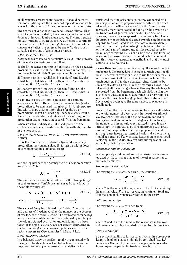
3.3.1. INTRODUCTIONThis model is suitable, for example, for some microbiologicalassays when the independent variable is the concentration ofan essential growth factor below the optimal concentrationof the medium. The slope-ratio model is illustrated inFigure 3.3.1.-I.
Figure 3.3.1.-I. – The slope-ratio model for a 2 × 3 + 1 assayThe doses are represented on the horizontal axis with zeroconcentration on the left and the highest concentration onthe right. The responses are indicated on the vertical axis.The individual responses to each treatment are indicatedwith black dots. The 2 lines are the calculated dose-responserelationship for the standard and the unknown under theassumption that they intersect each other at zero-dose.Unlike the parallel-line model, the doses are not transformedto logarithms.Just as in the case of an assay based on the parallel-linemodel, it is important that the assumed potency is close tothe true potency, and to prepare equipotent dilutions of thetest preparations and the standard (if feasible). The morenearly correct the assumed potency, the closer the 2 lineswill be together. The ratio of the slopes represents the “true”potency of the unknown, relative to its assumed potency. Ifthe slope of the unknown preparation is steeper than thatof the standard, the potency was underestimated and thecalculations will indicate an estimated potency higher thanthe assumed potency. Similarly, if the slope of the unknownis less steep than that of the standard, the potency wasoverestimated and the calculations will result in an estimatedpotency lower than the assumed potency.In setting up an experiment, all responses should beexamined for the fulfilment of the conditions 1, 2 and 3 inSection 3.1. The analysis of variance to be performed inroutine is described in Section 3.3.3 so that compliance withconditions 4B and 5B of Section 3.1 may be examined.
3.3.2. ASSAY DESIGNThe use of the statistical analysis presented below imposesthe following restrictions on the assay :a) the standard and the test preparations must be tested withthe same number of equally spaced dilutions,b) an extra group of experimental units receiving notreatment may be tested (the blanks),c) there must be an equal number of experimental units toeach treatment.
As already remarked in Section 3.1.3, assay designs notmeeting these restrictions may be both possible and correct,but the simple statistical analyses presented here are nolonger applicable and either expert advice should be soughtor suitable software should be used.A design with 2 doses per preparation and 1 blank, the“common zero (2h + 1)-design”, is usually preferred, since itgives the highest precision combined with the possibilityto check validity within the constraints mentioned above.However, a linear relationship cannot always be assumed tobe valid down to zero-dose. With a slight loss of precisiona design without blanks may be adopted. In this case3 doses per preparation, the “common zero (3h)-design”,are preferred to 2 doses per preparation. The doses are thusgiven as follows :1) the standard is given in a high dose, near to but notexceeding the highest dose giving a mean response on thestraight portion of the dose-response line,2) the other doses are uniformly spaced between the highestdose and zero dose,3) the test preparations are given in corresponding dosesbased on the assumed potency of the material.A completely randomised, a randomised block or aLatin square design may be used, such as described inSection 3.2.2. The use of any of these designs necessitatesan adjustment to the error sum of squares as described forassays based on the parallel-line model. The analysis of anassay of one or more test preparations against a standard isdescribed below.
3.3.3. ANALYSIS OF VARIANCE
3.3.3.1. The (hd + 1)-designThe responses are verified as described in Section 3.1and, if necessary, transformed. The responses are thenaveraged over each treatment and each preparation asshown in Table 3.3.3.1.-I. Additionally, the mean responsefor blanks (B) is calculated.The sums of squares in the analysis of variance are calculatedas shown in Tables 3.3.3.1.-I to 3.3.3.1.-III. The sum ofsquares due to non-linearity can only be calculated if at least3 doses of each preparation have been included in the assay.The residual error is obtained by subtracting the variationsallowed for in the design from the total variation in response(Table 3.3.3.1.-IV).The analysis of variance is now completed as follows. Eachsum of squares is divided by the corresponding number ofdegrees of freedom to give mean squares. The mean squarefor each variable to be tested is now expressed as a ratio tothe residual error (s2) and the significance of these values(known as F-ratios) are assessed by use of Table 8.1 or asuitable sub-routine of a computer program.
3.3.3.2. The (hd)-designThe formulae are basically the same as those for the(hd + 1)-design, but there are some slight differences.— B is discarded from all formulae.
—
— SSblank is removed from the analysis of variance.— The number of degrees of freedom for treatments becomes
hd − 1.— The number of degrees of freedom of the residual error
and the total variance is calculated as described for theparallel-line model (see Table 3.2.3.-IV).
Validity of the assay, potency and confidence interval arefound as described in Sections 3.3.4 and 3.3.5.
General Notices (1) apply to all monographs and other texts 577

5.3. Statistical analysis EUROPEAN PHARMACOPOEIA 6.0
Table 3.3.3.1.-I. — Formulae for slope-ratio assays with d doses of each preparation and a blank
Standard(S)
1st Test sample(T)
2nd Test sample(U, etc.)
Mean response lowest dose S1 T1 U1
Mean response 2nd dose S2 T2 U2
… … … …
Mean response highest dose Sd Td Ud
Total preparation
Linear product
Intercept value
Slope value
Treatment value
Non-linearity(*)
(*) Not calculated for two-dose assays
Table 3.3.3.1.-II. — Additional formulae for the construction of the analysis of variance
Table 3.3.3.1.-III. — Formulae to calculate the sum of squares and degrees of freedom
Source of variation Degrees of freedom (f) Sum of squares
Regression
Blanks
Intersection
Non-linearity(*)
Treatments
(*) Not calculated for two-dose assays
3.3.4. TESTS OF VALIDITYAssay results are said to be “statistically valid” if the outcomeof the analysis of variance is as follows :1) the variation due to blanks in (hd + 1)-designs is notsignificant, i.e. the calculated probability is not smaller than0.05. This indicates that the responses of the blanks do notsignificantly differ from the common intercept and the linearrelationship is valid down to zero dose ;2) the variation due to intersection is not significant, i.e. thecalculated probability is not less than 0.05. This indicatesthat condition 5B, Section 3.1 is satisfied ;3) in assays including at least 3 doses per preparation, thevariation due to non-linearity is not significant, i.e. thecalculated probability is not less than 0.05. This indicatesthat condition 4B, Section 3.1 is satisfied.A significant variation due to blanks indicates that thehypothesis of linearity is not valid near zero dose. If this islikely to be systematic rather than incidental for the type ofassay, the (hd-design) is more appropriate. Any response toblanks should then be disregarded.When these tests indicate that the assay is valid, the potencyis calculated with its confidence limits as described inSection 3.3.5.
3.3.5. ESTIMATION OF POTENCY AND CONFIDENCELIMITS
3.3.5.1. The (hd + 1)-designThe common intersection a′ of the preparations can becalculated from:
(3.3.5.1.-1)
The slope of the standard, and similarly for each of the otherpreparations, is calculated from:
(3.3.5.1.-2)
The potency ratio of each of the test preparations can nowbe calculated from:
(3.3.5.1.-3)
which has to be multiplied by AT, the assumed potency ofthe test preparation, in order to find the estimated potencyRT. If the step between adjacent doses was not identical
578 See the information section on general monographs (cover pages)

EUROPEAN PHARMACOPOEIA 6.0 5.3. Statistical analysis
Table 3.3.3.1.-IV. — Estimation of the residual error
Source of variation Degrees of freedom Sum of squares
Blocks (rows)(*)
Columns(**)
Completelyrandomised
Randomised blockResidual error(***)
Latin square
Total
For Latin square designs, these formulae are only applicable if n = hd(*) Not calculated for completely randomised designs(**) Only calculated for Latin square designs(***) Depends on the type of design
for the standard and the test preparation, the potency hasto be multiplied by IS/IT. Note that, unlike the parallel-lineanalysis, no antilogarithms are calculated.
The confidence interval for RT′ is calculated from:
(3.3.5.1.-4)
V1 are V2 are related to the variance and covariance of thenumerator and denominator of RT. They can be obtainedfrom:
(3.3.5.1.-5)
(3.3.5.1.-6)
The confidence limits are multiplied by AT, and if necessaryby IS/IT.
3.3.5.2. The (hd)-design
The formulae are the same as for the (hd + 1)-design, withthe following modifications :
(3.3.5.2.-1)
(3.3.5.2.-2)
(3.3.5.2.-3)
3.4. EXTENDED SIGMOID DOSE-RESPONSE CURVES
This model is suitable, for example, for some immunoassayswhen analysis is required of extended sigmoid dose-responsecurves. This model is illustrated in Figure 3.4.-I.
Figure 3.4.-I. – The four-parameter logistic curve modelThe logarithms of the doses are represented on thehorizontal axis with the lowest concentration on the left andthe highest concentration on the right. The responses areindicated on the vertical axis. The individual responses toeach treatment are indicated with black dots. The 2 curvesare the calculated ln(dose)-response relationship for thestandard and the test preparation.The general shape of the curves can usually be described bya logistic function but other shapes are also possible. Eachcurve can be characterised by 4 parameters : The upperasymptote (α), the lower asymptote (δ), the slope-factor (β),and the horizontal location (γ). This model is thereforeoften referred to as a four-parameter model. A mathematicalrepresentation of the ln(dose)-response curve is :
For a valid assay it is necessary that the curves of the standardand the test preparations have the same slope-factor, and thesame maximum and minimum response level at the extremeparts. Only the horizontal location (γ) of the curves maybe different. The horizontal distance between the curves isrelated to the “true” potency of the unknown. If the assayis used routinely, it may be sufficient to test the conditionof equal upper and lower response levels when the assay is
General Notices (1) apply to all monographs and other texts 579

5.3. Statistical analysis EUROPEAN PHARMACOPOEIA 6.0
developed, and then to retest this condition directly only atsuitable intervals or when there are changes in materials orassay conditions.
The maximum-likelihood estimates of the parameters andtheir confidence intervals can be obtained with suitablecomputer programs. These computer programs may includesome statistical tests reflecting validity. For example, if themaximum likelihood estimation shows significant deviationsfrom the fitted model under the assumed conditions of equalupper and lower asymptotes and slopes, then one or all ofthese conditions may not be satisfied.
The logistic model raises a number of statistical problemswhich may require different solutions for different types ofassays, and no simple summary is possible. A wide variety ofpossible approaches is described in the relevant literature.Professional advice is therefore recommended for this typeof analysis. A simple example is nevertheless included inSection 5.4 to illustrate a “possible” way to analyse the datapresented. A short discussion of alternative approaches andother statistical considerations is given in Section 7.5.
If professional advice or suitable software is not available,alternative approaches are possible : 1) if “reasonable”estimates of the upper limit (α) and lower limit (δ) areavailable, select for all preparations the doses with meanof the responses (u) falling between approximately 20 percent and 80 per cent of the limits, transform responses of
the selected doses to and use the parallel
line model (Section 3.2) for the analysis ; 2) select a range ofdoses for which the responses (u) or suitably transformedresponses, for example ln(u), are approximately linear whenplotted against ln(dose) ; the parallel line model (Section 3.2)may then be used for analysis.
4. ASSAYS DEPENDING UPONQUANTAL RESPONSES
4.1. INTRODUCTION
In certain assays it is impossible or excessively laboriousto measure the effect on each experimental unit on aquantitative scale. Instead, an effect such as death orhypoglycaemic symptoms may be observed as eitheroccurring or not occurring in each unit, and the resultdepends on the number of units in which it occurs. Suchassays are called quantal or all-or-none.
The situation is very similar to that described for quantitativeassays in Section 3.1, but in place of n separate responses toeach treatment a single value is recorded, i.e. the fractionof units in each treatment group showing a response.When these fractions are plotted against the logarithmsof the doses the resulting curve will tend to be sigmoid(S-shaped) rather than linear. A mathematical function thatrepresents this sigmoid curvature is used to estimate thedose-response curve. The most commonly used function isthe cumulative normal distribution function. This functionhas some theoretical merit, and is perhaps the best choiceif the response is a reflection of the tolerance of the units.If the response is more likely to depend upon a process ofgrowth, the logistic distribution model is preferred, althoughthe difference in outcome between the 2 models is usuallyvery small.
The maximum likelihood estimators of the slope and locationof the curves can be found only by applying an iterativeprocedure. There are many procedures which lead to thesame outcome, but they differ in efficiency due to the speedof convergence. One of the most rapid methods is directoptimisation of the maximum-likelihood function (seeSection 7.1), which can easily be performed with computerprograms having a built-in procedure for this purpose.Unfortunately, most of these procedures do not yield anestimate of the confidence interval, and the technique toobtain it is too complicated to describe here. The techniquedescribed below is not the most rapid, but has been chosenfor its simplicity compared to the alternatives. It can beused for assays in which one or more test preparationsare compared to a standard. Furthermore, the followingconditions must be fulfilled :
1) the relationship between the logarithm of the dose andthe response can be represented by a cumulative normaldistribution curve,
2) the curves for the standard and the test preparation areparallel, i.e. they are identically shaped and may only differin their horizontal location,
3) in theory, there is no natural response to extremely lowdoses and no natural non-response to extremely high doses.
4.2. THE PROBIT METHOD
The sigmoid curve can be made linear by replacing eachresponse, i.e. the fraction of positive responses per group, bythe corresponding value of the cumulative standard normaldistribution. This value, often referred to as “normit”, rangestheoretically from −∞ to + ∞. In the past it was proposedto add 5 to each normit to obtain “probits”. This facilitatedthe hand-performed calculations because negative valueswere avoided. With the arrival of computers the need toadd 5 to the normits has disappeared. The term “normitmethod” would therefore be better for the method describedbelow. However, since the term “probit analysis” is so widelyspread, the term will, for historical reasons, be maintained inthis text.
Once the responses have been linearised, it should bepossible to apply the parallel-line analysis as describedin Section 3.2. Unfortunately, the validity condition ofhomogeneity of variance for each dose is not fulfilled. Thevariance is minimal at normit = 0 and increases for positiveand negative values of the normit. It is therefore necessaryto give more weight to responses in the middle part of thecurve, and less weight to the more extreme parts of the curve.This method, the analysis of variance, and the estimation ofthe potency and confidence interval are described below.
4.2.1. TABULATION OF THE RESULTSTable 4.2.1.-I is used to enter the data into the columnsindicated by numbers :
(1) the dose of the standard or the test preparation,
(2) the number n of units submitted to that treatment,
(3) the number of units r giving a positive response to thetreatment,
(4) the logarithm x of the dose,
(5) the fraction p = r/n of positive responses per group.
The first cycle starts here.
(6) column Y is filled with zeros at the first iteration,
(7) the corresponding value = (Y) of the cumulativestandard normal distribution function (see also Table 8.4).
580 See the information section on general monographs (cover pages)

EUROPEAN PHARMACOPOEIA 6.0 5.3. Statistical analysis
The columns (8) to (10) are calculated with the followingformulae :
(8) (4.2.1.-1)
(9) (4.2.1.-2)
(10) (4.2.1.-3)
The columns (11) to (15) can easily be calculated fromcolumns (4), (9) and (10) as wx, wy, wx2, wy2 and wxyrespectively, and the sum ( ) of each of the columns (10) to(15) is calculated separately for each of the preparations.The sums calculated in Table 4.2.1.-I are transferred tocolumns (1) to (6) of Table 4.2.1.-II and 6 additional columns(7) to (12) are calculated as follows :
(7) (4.2.1.-4)
(8) (4.2.1.-5)
(9) (4.2.1.-6)
(10) (4.2.1.-7)
(11) (4.2.1.-8)
The common slope b can now be obtained as :
(4.2.1.-9)
and the intercept a of the standard, and similarly for the testpreparations is obtained as :
(12) (4.2.1.-10)
Column (6) of the first working table can now be replacedby Y = a + bx and the cycle is repeated until the differencebetween 2 cycles has become small (e.g. the maximumdifference of Y between 2 consecutive cycles is smallerthan 10−8).
4.2.2. TESTS OF VALIDITYBefore calculating the potencies and confidence intervals,validity of the assay must be assessed. If at least 3 doses foreach preparation have been included, the deviations fromlinearity can be measured as follows : add a 13th column toTable 4.2.1.-II and fill it with :
(4.2.2.-1)
The column total is a measure of deviations from linearity andis approximately χ2 distributed with degrees of freedom equalto N −2h. Significance of this value may be assessed withthe aid of Table 8.3 or a suitable sub-routine in a computerprogram. If the value is significant at the 0.05 probabilitylevel, the assay must probably be rejected (see Section 4.2.4).
When the above test gives no indication of significantdeviations from linear regression, the deviations fromparallelism are tested at the 0.05 significance level with :
(4.2.2.-2)
with h − 1 degrees of freedom.
4.2.3. ESTIMATION OF POTENCY AND CONFIDENCELIMITSWhen there are no indications for a significant departurefrom parallelism and linearity the ln(potency ratio) M′T iscalculated as :
(4.2.3.-1)
Table 4.2.1.-I. — First working table
(1) (2) (3) (4) (5) (6) (7) (8) (9) (10) (11) (12) (13) (14) (15)
dose n r x p Y Z y w wx wy wx2 wy2 wxy
S . . . . . . . . . . . . . . .
. . . . . . . . . . . . . . .
. . . . . . . . . . . . . . .
= = = = = =
T . . . . . . . . . . . . . . .
. . . . . . . . . . . . . . .
. . . . . . . . . . . . . . .
= = = = = =
etc.
Table 4.2.1.-II. — Second working table
(1) (2) (3) (4) (5) (6) (7) (8) (9) (10) (11) (12)
w wx wy wx2 wy2 wxy Sxx Sxy Syya
S . . . . . . . . . . . .
T . . . . . . . . . . . .
etc. . . . . . . . . . . . .
= =
General Notices (1) apply to all monographs and other texts 581

5.3. Statistical analysis EUROPEAN PHARMACOPOEIA 6.0
and the antilogarithm is taken. Now let t = 1.96 and s = 1.Confidence limits are calculated as the antilogarithms of :
(4.2.3.-2)
4.2.4. INVALID ASSAYSIf the test for deviations from linearity described inSection 4.2.2 is significant, the assay should normally berejected. If there are reasons to retain the assay, the formulaeare slightly modified. t becomes the t-value (p = 0.05) withthe same number of degrees of freedom as used in the checkfor linearity and s2 becomes the χ2 value divided by the samenumber of degrees of freedom (and thus typically is greaterthan 1).
The test for parallelism is also slightly modified. The χ2
value for non-parallelism is divided by its number of degreesof freedom. The resulting value is divided by s2 calculatedabove to obtain an F-ratio with h - 1 and N - 2h degrees offreedom, which is evaluated in the usual way at the 0.05significance level.
4.3. THE LOGIT METHOD
As indicated in Section 4.1 the logit method may sometimesbe more appropriate. The name of the method is derivedfrom the logit function which is the inverse of the logisticdistribution. The procedure is similar to that described forthe probit method with the following modifications in theformulae for and Z.
(4.3.-1)
(4.3.-2)
4.4. OTHER SHAPES OF THE CURVE
The probit and logit method are almost always adequate forthe analysis of quantal responses called for in the EuropeanPharmacopoeia. However, if it can be made evident that theln(dose)-response curve has another shape than the 2 curvesdescribed above, another curve may be adopted. Z is thentaken to be the first derivative of .
For example, if it can be shown that the curve is not symmetric,the Gompertz distribution may be appropriate (the gompitmethod) in which case .
4.5. THE MEDIAN EFFECTIVE DOSE
In some types of assay it is desirable to determine a medianeffective dose which is the dose that produces a response in50 per cent of the units. The probit method can be used todetermine this median effective dose (ED50), but since thereis no need to express this dose relative to a standard, theformulae are slightly different.
Note : a standard can optionally be included in order tovalidate the assay. Usually the assay is considered valid ifthe calculated ED50 of the standard is close enough to theassigned ED50. What “close enough” in this context meansdepends on the requirements specified in the monograph.
The tabulation of the responses to the test samples, andoptionally a standard, is as described in Section 4.2.1. Thetest for linearity is as described in Section 4.2.2. A test for
parallelism is not necessary for this type of assay. The ED50of test sample T, and similarly for the other samples, isobtained as described in Section 4.2.3, with the followingmodifications in formulae 4.2.3.-1 and 4.2.3.-2).
(4.5.-1)
(4.5.-2)
where and C is left unchanged
5. EXAMPLESThis section consists of worked examples illustrating theapplication of the formulae. The examples have beenselected primarily to illustrate the statistical method ofcalculation. They are not intended to reflect the mostsuitable method of assay, if alternatives are permitted in theindividual monographs. To increase their value as programchecks, more decimal places are given than would usually benecessary. It should also be noted that other, but equivalentmethods of calculation exist. These methods should lead toexactly the same final results as those given in the examples.
5.1. PARALLEL-LINE MODEL
5.1.1. TWO-DOSE MULTIPLE ASSAY WITH COMPLETELYRANDOMISED DESIGNAn assay of corticotrophin by subcutaneous injection inrats
The standard preparation is administered at 0.25 and1.0 units per 100 g of body mass. 2 preparations to beexamined are both assumed to have a potency of 1 unit permilligram and they are administered in the same quantitiesas the standard. The individual responses and means pertreatment are given in Table 5.1.1.-I. A graphical presentation(Figure 5.1.1.-I) gives no rise to doubt the homogeneity ofvariance and normality of the data, but suggests problemswith parallelism for preparation U.
Table 5.1.1.-I. — Response metameter y : mass of ascorbicacid (mg) per 100 g of adrenal gland
Standard S Preparation T Preparation U
S1 S2 T1 T2 U1 U2
300 289 310 230 250 236
310 221 290 210 268 213
330 267 360 280 273 283
290 236 341 261 240 269
364 250 321 241 307 251
328 231 370 290 270 294
390 229 303 223 317 223
360 269 334 254 312 250
342 233 295 216 320 216
306 259 315 235 265 265
Mean 332.0 248.4 323.9 244.0 282.2 250.0
582 See the information section on general monographs (cover pages)

EUROPEAN PHARMACOPOEIA 6.0 5.3. Statistical analysis
Figure 5.1.1.-I.
The formulae in Tables 3.2.3.-I and 3.2.3.-II lead to :
PS= 580.4 LS
= −41.8
PT= 567.9 LT
= −39.95
PU= 532.2 LU
= −16.1
HP = = 5 HL = = 20
The analysis of variance can now be completed with theformulae in Tables 3.2.3-III and 3.2.3.-IV. This is shown inTable 5.1.1.-II.
Table 5.1.1.-II. — Analysis of variance
Source ofvariation
Degrees offreedom
Sum ofsquares
Meansquare F-ratio
Proba-bility
Preparations 2 6256.6 3128.3
Regression 1 63 830.8 63 830.8 83.38 0.000
Non-parallelism 2 8218.2 4109.1 5.37 0.007
Treatments 5 78 305.7
Residual error 54 41 340.9 765.57
Total 59 119 646.6
The analysis confirms a highly significant linear regression.Departure from parallelism, however, is also significant(p = 0.0075) which was to be expected from the graphicalobservation that preparation U is not parallel to thestandard. This preparation is therefore rejected and theanalysis repeated using only preparation T and the standard(Table 5.1.1.-III).
Table 5.1.1.-III. — Analysis of variance without sample U
Source ofvariation
Degrees offreedom
Sum ofsquares
Meansquare F-ratio
Proba-bility
Preparations 1 390.6 390.6
Regression 1 66 830.6 66 830.6 90.5 0.000
Non-parallelism 1 34.2 34.2 0.05 0.831
Treatments 3 67 255.5
Residual error 36 26 587.3 738.54
Total 39 93 842.8
The analysis without preparation U results in compliancewith the requirements with respect to both regressionand parallelism and so the potency can be calculated. Theformulae in Section 3.2.5 give :
— for the common slope :
— the ln(potency ratio) is :
— and ln(confidence limits) are :
By taking the antilogarithms we find a potency ratio of 1.11with 95 per cent confidence limits from 0.82-1.51.
Multiplying by the assumed potency of preparation T yields apotency of 1.11 units/mg with 95 per cent confidence limitsfrom 0.82 to 1.51 units/mg.
5.1.2. THREE-DOSE LATIN SQUARE DESIGNAntibiotic agar diffusion assay using a rectangular tray
The standard has an assigned potency of 4855 IU/mg. Thetest preparation has an assumed potency of 5600 IU/mg.For the stock solutions 25.2 mg of the standard is dissolvedin 24.5 ml of solvent and 21.4 mg of the test preparationis dissolved in 23.95 ml of solvent. The final solutions areprepared by first diluting both stock solutions to 1/20 andfurther using a dilution ratio of 1.5.
A Latin square is generated with the method describedin Section 8.6 (see Table 5.1.2.-I). The responses of thisroutine assay are shown in Table 5.1.2.-II (inhibition zonesin mm × 10). The treatment mean values are shown inTable 5.1.2.-III. A graphical representation of the data (seeFigure 5.1.2.-I) gives no rise to doubt the normality orhomogeneity of variance of the data.
The formulae in Tables 3.2.3.-I and 3.2.3.-II lead to :
P S= 529.667 L S
= 35.833
P T= 526.333 L T
= 39.333
H P = = 2 H L = = 3
The analysis of variance can now be completed with theformulae in Tables 3.2.3.-III and 3.2.3.-IV. The result is shownin Table 5.1.2.-IV.
The analysis shows significant differences between the rows.This indicates the increased precision achieved by using aLatin square design rather than a completely randomiseddesign. A highly significant regression and no significantdeparture of the individual regression lines from parallelismand linearity confirms that the assay is satisfactory forpotency calculations.
General Notices (1) apply to all monographs and other texts 583

5.3. Statistical analysis EUROPEAN PHARMACOPOEIA 6.0
Table 5.1.2.-I. — Distribution of treatments over the plate
1 2 3 4 5 6
1 S1 T1 T2 S3 S2 T3
2 T1 T3 S1 S2 T2 S3
3 T2 S3 S2 S1 T3 T1
4 S3 S2 T3 T1 S1 T2
5 S2 T2 S3 T3 T1 S1
6 T3 S1 T1 T2 S3 S2
Table 5.1.2.-II. — Measured inhibition zones in mm × 10
1 2 3 4 5 6 Row mean
1 161 160 178 187 171 194 175.2 = R1
2 151 192 150 172 170 192 171.2 = R2
3 162 195 174 161 193 151 172.7 = R3
4 194 184 199 160 163 171 178.5 = R4
5 176 181 201 202 154 151 177.5 = R5
6 193 166 161 186 198 182 181.0 = R6
Col.Mean
172.8= C1
179.7= C2
177.2= C3
178.0= C4
174.8= C5
173.5= C6
Table 5.1.2.-III. — Means of the treatments
Standard S Preparation T
S1 S2 S3 T1 T2 T3
Mean 158.67 176.50 194.50 156.17 174.67 195.50
Figure 5.1.2.-I.
Table 5.1.2.-IV. — Analysis of variance
Source ofvariation
Degrees offreedom
Sum ofsquares
Meansquare F-ratio Probabil-
ity
Preparations 1 11.1111 11.1111
Regression 1 8475.0417 8475.0417 408.1 0.000
Non-parallelism 1 18.3750 18.3750 0.885 0.358
Non-linearity 2 5.4722 2.7361 0.132 0.877
Treatments 5 8510
Rows 5 412 82.40 3.968 0.012
Columns 5 218.6667 43.73 2.106 0.107
Residual error 20 415.3333 20.7667
Total 35 9556
The formulae in Section 3.2.5 give :
— for the common slope :
— the ln(potency ratio) is :
— and ln(confidence limits) are :
The potency ratio is found by taking the antilogarithms,resulting in 0.9763 with 95 per cent confidence limits from0.9112-1.0456.
A correction factor of is
necessary because the dilutions were not exactly equipotenton the basis of the assumed potency. Multiplying by thiscorrection factor and the assumed potency of 5600 IU/mgyields a potency of 5456 IU/mg with 95 per cent confidencelimits from 5092 to 5843 IU/mg.
5.1.3. FOUR-DOSE RANDOMISED BLOCK DESIGNAntibiotic turbidimetric assay
This assay is designed to assign a potency in internationalunits per vial. The standard has an assigned potency of670 IU/mg. The test preparation has an assumed potency of20 000 IU/vial. On the basis of this information the stocksolutions are prepared as follows. 16.7 mg of the standardis dissolved in 25 ml solvent and the contents of one vialof the test preparation are dissolved in 40 ml solvent. Thefinal solutions are prepared by first diluting to 1/40 andfurther using a dilution ratio of 1.5. The tubes are placedin a water-bath in a randomised block arrangement (seeSection 8.5). The responses are listed in Table 5.1.3.-I.
Inspection of Figure 5.1.3.-I gives no rise to doubt the validityof the assumptions of normality and homogeneity of varianceof the data. The standard deviation of S3 is somewhat highbut is no reason for concern.
584 See the information section on general monographs (cover pages)

EUROPEAN PHARMACOPOEIA 6.0 5.3. Statistical analysis
Table 5.1.3.-I. — Absorbances of the suspensions (× 1000)
Standard S Preparation T
Block S1 S2 S3 S4 T1 T2 T3 T4 Mean
1 252 207 168 113 242 206 146 115 181.1
2 249 201 187 107 236 197 153 102 179.0
3 247 193 162 111 246 197 148 104 176.0
4 250 207 155 108 231 191 159 106 175.9
5 235 207 140 98 232 186 146 95 167.4
Mean 246.6 203.0 162.4 107.4 237.4 195.4 150.4 104.4
Figure 5.1.3.-I.
The formulae in Tables 3.2.3.-I and 3.2.3.-II lead to :
PS= 719.4 LS
= −229.1
PT= 687.6 LT
= −222
HP = = 1.25 HL = = 1
The analysis of variance is constructed with the formulaein Tables 3.2.3.-III and 3.2.3.-IV. The result is shown inTable 5.1.3.-II.
Table 5.1.3.-II. — Analysis of variance
Source ofvariation
Degrees offreedom
Sum ofsquares
Mean square F-ratio Proba-bility
Preparations 1 632.025 632.025
Regression 1 101 745.6 101 745.6 1887.1 0.000
Non-parallelism 1 25.205 25.205 0.467 0.500
Non-linearity 4 259.14 64.785 1.202 0.332
Treatments 7 102 662
Blocks 4 876.75 219.188 4.065 0.010
Residual error 28 1509.65 53.916
Total 39 105 048.4
A significant difference is found between the blocks. Thisindicates the increased precision achieved by using arandomised block design. A highly significant regression
and no significant departure from parallelism andlinearity confirms that the assay is satisfactory for potencycalculations. The formulae in Section 3.2.5 give :
— for the common slope :
— the ln(potency ratio) is :
— and ln(confidence limits) are :
The potency ratio is found by taking the antilogarithms,resulting in 1.0741 with 95 per cent confidencelimits from 1.0291 to 1.1214. A correction factor of
is necessary because the
dilutions were not exactly equipotent on the basis of theassumed potency. Multiplying by this correction factor andthe assumed potency of 20 000 IU/vial yields a potencyof 19 228 IU/vial with 95 per cent confidence limits from18 423-20 075 IU/vial.
5.1.4. FIVE-DOSEMULTIPLE ASSAYWITH COMPLETELYRANDOMISED DESIGNAn in-vitro assay of three hepatitis B vaccines against astandard
3 independent two-fold dilution series of 5 dilutions wereprepared from each of the vaccines. After some additionalsteps in the assay procedure, absorbances were measured.They are shown in Table 5.1.4.-I.
Table 5.1.4.-I. — Optical densities
Dilution Standard S Preparation T
1:16 000 0.043 0.045 0.051 0.097 0.097 0.094
1:8000 0.093 0.099 0.082 0.167 0.157 0.178
1:4000 0.159 0.154 0.166 0.327 0.355 0.345
1:2000 0.283 0.295 0.362 0.501 0.665 0.576
1:1000 0.514 0.531 0.545 1.140 1.386 1.051
Dilution Preparation U Preparation V
1:16 000 0.086 0.071 0.073 0.082 0.082 0.086
1:8000 0.127 0.146 0.133 0.145 0.144 0.173
1:4000 0.277 0.268 0.269 0.318 0.306 0.316
1:2000 0.586 0.489 0.546 0.552 0.551 0.624
1:1000 0.957 0.866 1.045 1.037 1.039 1.068
The logarithms of the optical densities are known to havea linear relationship with the logarithms of the doses. Themean responses of the ln-transformed optical densities arelisted in Table 5.1.4.-II. No unusual features are discoveredin a graphical presentation of the data (Figure 5.1.4.-I).
General Notices (1) apply to all monographs and other texts 585

5.3. Statistical analysis EUROPEAN PHARMACOPOEIA 6.0
Table 5.1.4.-II. — Means of the ln-transformed absorbances
S1 −3.075 T1 −2.344 U1 −2.572 V1 −2.485
S2 −2.396 T2 −1.789 U2 −2.002 V2 −1.874
S3 −1.835 T3 −1.073 U3 −1.305 V3 −1.161
S4 −1.166 T4 −0.550 U4 −0.618 V4 −0.554
S5 −0.635 T5 0.169 U5 −0.048 V5 0.047
Figure 5.1.4.-I.
The formulae in Tables 3.2.3.-I and 3.2.3.-II give :
PS= −9.108 LS
= 6.109
PT= −5.586 LT
= 6.264
PU= −6.544 LU
= 6.431
PV= −6.027 LV
= 6.384
HP = = 0.6 HL = = 0.3
The analysis of variance is completed with the formulae inTables 3.2.3.-III and 3.2.3.-IV. This is shown in Table 5.1.4.-III.
Table 5.1.4.-III. — Analysis of variance
Source ofvariation
Degrees offreedom
Sum ofsquares
Meansquare F-ratio Probabil-
ity
Preparations 3 4.475 1.492
Regression 1 47.58 47.58 7126 0.000
Non-parallelism
3 0.0187 0.006 0.933 0.434
Non-linearity 12 0.0742 0.006 0.926 0.531
Treatments 19 52.152
Residual error 40 0.267 0.0067
Total 59 52.42
A highly significant regression and a non-significantdeparture from parallelism and linearity confirm thatthe potencies can be safely calculated. The formulae inSection 3.2.5 give :
— for the common slope :
— the ln(potency ratio) for preparation T is :
— and ln(confidence limits) for preparation T are :
By taking the antilogarithms a potency ratio of 2.171 isfound with 95 per cent confidence limits from 2.027 to 2.327.All samples have an assigned potency of 20 µg protein/mland so a potency of 43.4 µg protein/ml is found for testpreparation T with 95 per cent confidence limits from40.5-46.5 µg protein/ml.The same procedure is followed to estimate the potencyand confidence interval of the other test preparations. Theresults are listed in Table 5.1.4.-IV.
Table 5.1.4.-IV. — Final potency estimates and 95 per centconfidence intervals of the test vaccines (in µg protein/ml)
Lower limit Estimate Upper limit
Vaccine T 40.5 43.4 46.5
Vaccine U 32.9 35.2 37.6
Vaccine V 36.8 39.4 42.2
5.1.5. TWIN CROSS-OVER DESIGNAssay of insulin by subcutaneous injection in rabbitsThe standard preparation was administered at 1 unit and2 units per millilitre. Equivalent doses of the unknownpreparation were used based on an assumed potency of 40units per millilitre. The rabbits received subcutaneously0.5 ml of the appropriate solutions according to thedesign in Table 5.1.5.-I and responses obtained are shownin Table 5.1.5.-II and Figure 5.1.5.-I. The large varianceillustrates the variation between rabbits and the need toemploy a cross-over design.
Table 5.1.5.-I. — Arrangements of treatments
Group of rabbits
1 2 3 4
Day 1 S1 S2 T1 T2
Day 2 T2 T1 S2 S1
Table 5.1.5.-II. — Response y: sum of blood glucosereadings (mg/100 ml) at 1 hour and hours
Group 1 Group 2 Group 3 Group 4
S1 T2 S2 T1 T1 S2 T2 S1
112 104 65 72 105 91 118 144
126 112 116 160 83 67 119 149
62 58 73 72 125 67 42 51
86 63 47 93 56 45 64 107
52 53 88 113 92 84 93 117
110 113 63 71 101 56 73 128
116 91 50 65 66 55 39 87
101 68 55 100 91 68 31 71
Mean 95.6 82.8 69.6 93.3 89.9 66.6 72.4 106.8
586 See the information section on general monographs (cover pages)

EUROPEAN PHARMACOPOEIA 6.0 5.3. Statistical analysis
Figure 5.1.5.-I.
The analysis of variance is more complicated for this assaythan for the other designs given because the component ofthe sum of squares due to parallelism is not independentof the component due to rabbit differences. Testing ofthe parallelism of the regression lines involves a seconderror-mean-square term obtained by subtracting theparallelism component and 2 “interaction” components fromthe component due to rabbit differences.
3 “interaction” components are present in the analysis ofvariance due to replication within each group:
days × preparation ; days × regression ; days × parallelism.
These terms indicate the tendency for the components(preparations, regression and parallelism) to vary from dayto day. The corresponding F-ratios thus provide checks onthese aspects of assay validity. If the values of F obtained aresignificantly high, care should be exercised in interpretingthe results of the assay and, if possible, the assay should berepeated.
The analysis of variance is constructed by applying theformulae given in Tables 3.2.3.-I to 3.2.3.-III separately forboth days and for the pooled set of data. The formulae inTables 3.2.3.-I and 3.2.3.-II give :
Day 1 : PS= 165.25 LS
= −13
PT= 162.25 LT
= −8.75
HP= HL
=
Day 2 : PS= 173.38 LS
= −20.06
PT= 176.00 LT
= −5.25
HP= HL
=
Pooled : PS= 169.31 LS
= −16.53
PT= 169.13 LT
= −7.00
HP = HL=
and with the formulae in Table 3.2.3.-III this leads to :
Day 1 Day 2 Pooled
SSprep = 18.000 SSprep= 13.781 SSprep
= 0.141
SSreg= 3784.5 SSreg
= 5125.8 SSreg= 8859.5
SSpar = 144.5 SSpar= 1755.3 SSpar
= 1453.5
The interaction terms are found as Day 1 + Day 2 - Pooled.
In addition the sum of squares due to day-to-day variationis calculated as :
and the sum of squares due to blocks (the variation betweenrabbits) as :
where Bi is the mean response per rabbit.
The analysis of variance can now be completed as shownin Table 5.1.5.-III.
Table 5.1.5.-III. — Analysis of variance
Source ofvariation
Degreesof
freedom
Sum ofsquares
Meansquare F-ratio
Proba-bility
Non-parallelism
1 1453.5 1453.5 1.064 0.311
Days × Prep. 1 31.6 31.6 0.023 0.880
Days × Regr. 1 50.8 50.8 0.037 0.849
Residualerror betweenrabbits
28 38 258.8 1366.4
Rabbits 31 39 794.7 1283.7
Preparations 1 0.14 0.14 0.001 0.975
Regression 1 8859.5 8859.5 64.532 0.000
Days 1 478.5 478.5 3.485 0.072
Days × non-par.
1 446.3 446.3 3.251 0.082
Residualerror withinrabbits
28 3844.1 137.3
Total 63 53 423.2
The analysis of variance confirms that the data fulfil thenecessary conditions for a satisfactory assay : a highlysignificant regression, no significant departures fromparallelism, and none of the three interaction componentsis significant.
The formulae in Section 3.2.5 give :
— for the common slope :
— the ln(potency ratio) is :
General Notices (1) apply to all monographs and other texts 587

5.3. Statistical analysis EUROPEAN PHARMACOPOEIA 6.0
— and ln(confidence limits) are :
By taking the antilogarithms a potency ratio of 1.003with 95 per cent confidence limits from 0.835 to 1.204is found. Multiplying by AT = 40 yields a potency of 40.1units per millilitre with 95 per cent confidence limits from33.4-48.2 units per millilitre.
5.2. SLOPE-RATIO MODEL
5.2.1. A COMPLETELY RANDOMISED (0,3,3)-DESIGNAn assay of factor VIII
A laboratory carries out a chromogenic assay of factor VIIIactivity in concentrates. The laboratory has no experiencewith the type of assay but is trying to make it operational.3 equivalent dilutions are prepared of both the standardand the test preparation. In addition a blank is prepared,although a linear dose-response relationship is not expectedfor low doses. 8 replicates of each dilution are prepared,which is more than would be done in a routine assay.
A graphical presentation of the data shows clearly that thedose-response relationship is indeed not linear at low doses.The responses to blanks will therefore not be used in thecalculations (further assays are of course needed to justifythis decision). The formulae in Tables 3.3.3.1.-I and 3.3.3.1.-IIyield
PS= 0.6524 PT
= 0.5651
LS= 1.4693 LT
= 1.2656
aS = 0.318 aT = 0.318
bS = 0.329 bT = 0.271
GS= 0.1554 GT
= 0.1156
JS = 4.17 · 10−8 JT = 2.84 · 10−6
and
HI= 0.09524 a′ = 0.05298 K = 1.9764
and the analysis of variance is completed with the formulaein Tables 3.3.3.1.-III and 3.3.3.1.-IV.
A highly significant regression and no significant deviationsfrom linearity and intersection indicate that the potency canbe calculated.
Slope of standard :
Slope of test sample :
Formula 3.3.5.1.-3 gives :
and the 95 per cent confidence limits are :
The potency ratio is thus estimated as 0.823 with 95 per centconfidence limits from 0.817 to 0.829.
Table 5.2.1.-I. — Absorbances
Blank Standard S(in IU/ml)
Preparation T(in IU/ml)
Conc. B S1
0.01S2
0.02S3
0.03T1
0.01T2
0.02T3
0.03
0.022 0.133 0.215 0.299 0.120 0.188 0.254
0.024 0.133 0.215 0.299 0.119 0.188 0.253
0.024 0.131 0.216 0.299 0.118 0.190 0.255
0.026 0.136 0.218 0.297 0.120 0.190 0.258
0.023 0.137 0.220 0.297 0.120 0.190 0.257
0.022 0.136 0.220 0.305 0.121 0.191 0.257
0.022 0.138 0.219 0.299 0.121 0.191 0.255
0.023 0.137 0.218 0.302 0.121 0.190 0.254
Mean 0.0235 0.1351 0.2176 0.2996 0.1200 0.1898 0.2554
Figure 5.2.1.-I.
Table 5.2.1.-II. — Analysis of variance
Source ofvariation
Degreesof
freedom
Sum ofsquares
Meansquare F-ratio Probabil-
ity
Regression 2 0.1917 0.0958 24 850 0.000
Intersection 1 3 · 10−9 3 · 10−9 7 · 10−4 0.978
Non-linearity 2 2 · 10−5 1 · 10−5 2.984 0.061
Treatments 5 0.1917
Residual error 42 1.62 · 10−4 3.86 · 10−6
Total 47 0.1919
5.2.2. A COMPLETELY RANDOMISED (0,4,4,4)-DESIGNAn in-vitro assay of influenza vaccinesThe haemagglutinin antigen (HA) content of 2 influenzavaccines is determined by single radial immunodiffusion.Both have a labelled potency of 15 µg HA per dose, which isequivalent with a content of 30 µg HA/ml. The standard hasan assigned content of 39 µg HA/ml.Standard and test vaccines are applied in 4 duplicateconcentrations which are prepared on the basis of theassigned and the labelled contents. When the equilibriumbetween the external and the internal reactant is established,the zone of the annulus precipitation area is measured. Theresults are shown in Table 5.2.2.-I.
588 See the information section on general monographs (cover pages)

EUROPEAN PHARMACOPOEIA 6.0 5.3. Statistical analysis
Table 5.2.2.-I. — Zone of precipitation area (mm2)
Conc. Standard S Preparation T Preparation U
( µg/ml) I II I II I II
7.5 18.0 18.0 15.1 16.8 15.4 15.7
15.0 22.8 24.5 23.1 24.2 20.2 18.6
22.5 30.4 30.4 28.9 27.4 24.2 23.1
30.0 35.7 36.6 34.4 37.8 27.4 27.0
A graphical presentation of the data shows no unusualfeatures (see Figure 5.2.2.-I). The formulae in Tables 3.3.3.1.-Iand 3.3.3.1.-II yield
PS= 108.2 PT
= 103.85 PU= 85.8
LS= 301.1 LT
= 292.1 LU= 234.1
aS = 141.0 aT = 116.7 aU = 139.8
bS = 61.2 bT = 64.95 bU = 39.2
GS= 3114.3 GT
= 2909.4 GU= 1917.3
JS = 0.223 JT = 2.227 JU = 0.083
and
HI= 0.0093 a′ = 11.04 K = 14 785.8
and the analysis of variance is completed with the formulaein Tables 3.3.3.1.-III and 3.3.3.1.-IV. This is shown inTable 5.2.2.-II.
A highly significant regression and no significant deviationsfrom linearity and intersection indicate that the potency canbe calculated.
Slope of standard :
Slope of T is :
Slope of U is :
This leads to a potency ratio of 6.056/6.356 = 0.953 forvaccine T and 4.123/6.356 = 0.649 for vaccine U.
And the confidence limits are found with formula 3.3.5.1.-4.
For vaccine T :
For vaccine U :
The HA content in µg/dose can be found by multiplying thepotency ratios and confidence limits by the assumed contentof 15 µg/dose. The results are given in Table 5.2.2.-III.
Figure 5.2.2.-I.
Table 5.2.2.-II. — Analysis of variance
Source ofvariation
Degreesof
freedom
Sum ofsquares
Meansquare F-ratio Probabil-
ity
Regression 3 1087.7 362.6 339.5 0.000
Intersection 2 3.474 1.737 1.626 0.237
Non-linearity 6 5.066 0.844 0.791 0.594
Treatments 11 1096.2
Residual error 12 12.815 1.068
Total 23 1109.0
Table 5.2.2.-III. — Estimates of HA content (µg/dose)
Lower limit Estimate Upper limit
Vaccin T 13.4 14.3 15.3
Vaccin U 8.9 9.7 10.6
5.3. QUANTAL RESPONSES
5.3.1. PROBIT ANALYSIS OF A TEST PREPARATIONAGAINST A REFERENCEAn in-vivo assay of a diphtheria vaccineA diphtheria vaccine (assumed potency 140 IU/vial) isassayed against a standard (assigned potency 132 IU/vial).On the basis of this information, equivalent dosesare prepared and randomly administered to groups ofguinea-pigs. After a given period, the animals are challengedwith diphtheria toxin and the number of surviving animalsrecorded as shown in Table 5.3.1.-I.
Table 5.3.1.-I. — Raw data from a diphtheria assay inguinea-pigs
Standard (S)Assigned potency
132 IU/vial
Test preparation (T)Assumed potency
140 IU/vial
dose(IU/ml)
chal-lenged
protect-ed
dose(I.U./ml)
chal-lenged
protect-ed
1.0 12 0 1.0 11 0
1.6 12 3 1.6 12 4
2.5 12 6 2.5 11 8
4.0 11 10 4.0 11 10
General Notices (1) apply to all monographs and other texts 589

5.3. Statistical analysis EUROPEAN PHARMACOPOEIA 6.0
The observations are transferred to the first working tableand the subsequent columns are computed as described inSection 4.2.1. Table 5.3.1.-II shows the first cycle of thisprocedure.
The sums of the last 6 columns are then calculated perpreparation and transferred to the second working table (seeTable 5.3.1.-III). The results in the other columns are foundwith formulae 4.2.1.-4 to 4.2.1.-10. This yields a commonslope b of 1.655.
The values for Y in the first working table are now replaced bya + bx and a second cycle is carried out (see Table 5.3.1.-IV).
The cycle is repeated until the difference between2 consecutive cycles has become small. The second workingtable should then appear as shown in Table 5.3.1.-V.
Linearity is tested as described in Section 4.2.2. Theχ2-value with 4 degrees of freedom is 0.851 + 1.070 = 1.921representing a p-value of 0.750 which is not significant.
Since there are no significant deviations from linearity, thetest for parallelism can be carried out as described in thesame section. The χ2-value with 1 degree of freedom is
representing a p-valueof 0.974 which is not significant.The ln(potency ratio) can now be estimated as described inSection 4.2.3.
Further :
So ln confidence limits are :
The potency and confidence limits can now be found bytaking the antilogarithms and multiplying these by theassumed potency of 140 IU/vial. This yields an estimateof 160.6 IU/vial with 95 per cent confidence limits from121.0-215.2 IU/vial.
Table 5.3.1.-II. — First working table in the first cycle
Vac-cine Dose n r x p Y Z y w wx wy wx2 wy2 wxy
S 1.0 12 0 0.000 0.000 0 0.5 0.399 −1.253 7.64 0.00 −9.57 0.00 12.00 0.00
1.6 12 3 0.470 0.250 0 0.5 0.399 −0.627 7.64 3.59 −4.79 1.69 3.00 −2.25
2.5 12 6 0.916 0.500 0 0.5 0.399 0.000 7.64 7.00 0.00 6.41 0.00 0.00
4.0 11 10 1.386 0.909 0 0.5 0.399 1.025 7.00 9.71 7.18 13.46 7.36 9.95
T 1.0 11 0 0.000 0.000 0 0.5 0.399 −1.253 7.00 0.00 −8.78 0.00 11.00 0.00
1.6 12 4 0.470 0.333 0 0.5 0.399 −0.418 7.64 3.59 −3.19 1.69 1.33 −1.50
2.5 11 8 0.916 0.727 0 0.5 0.399 0.570 7.00 6.42 3.99 5.88 2.27 3.66
4.0 11 10 1.386 0.909 0 0.5 0.399 1.025 7.00 9.71 7.18 13.46 7.36 9.95
Table 5.3.1.-III. — Second working table in the first cycle
Vaccine w wx wy wx2 wy2 wxy Sxx Sxy Syya
S 29.92 20.30 −7.18 21.56 22.36 7.70 7.79 12.58 20.64 0.68 −0.24 −1.36
T 28.65 19.72 −0.80 21.03 21.97 12.11 7.46 12.66 21.95 0.69 −0.03 −1.17
Table 5.3.1.-IV. — First working table in the second cycle
Vac-cine Dose n r x p Y Z y w wx wy wx2 wy2 wxy
S 1.0 12 0 0.000 0.000 −1.36 0.086 0.158 −1.911 3.77 0.00 −7.21 0.00 13.79 0.00
1.6 12 3 0.470 0.250 −0.58 0.279 0.336 −0.672 6.74 3.17 −4.53 1.49 3.04 −2.13
2.5 12 6 0.916 0.500 0.15 0.561 0.394 −0.001 7.57 6.94 −0.01 6.36 0.00 −0.01
4.0 11 10 1.386 0.909 0.93 0.824 0.258 1.260 5.07 7.03 6.39 9.75 8.05 8.86
T 1.0 11 0 0.000 0.000 −1.17 0.122 0.202 −1.769 4.20 0.00 −7.43 0.00 13.14 0.00
1.6 12 4 0.470 0.333 −0.39 0.349 0.370 −0.430 7.23 3.40 −3.11 1.60 1.34 −1.46
2.5 11 8 0.916 0.727 0.35 0.637 0.375 0.591 6.70 6.14 3.96 5.62 2.34 3.63
4.0 11 10 1.386 0.909 1.13 0.870 0.211 1.311 4.35 6.03 5.70 8.36 7.48 7.90
Table 5.3.1.-V. — Second working table after sufficient cycles
Vaccine w wx wy wx2 wy2 wxy Sxx Sxy Syya
S 18.37 14.80 −2.14 14.85 17.81 5.28 2.93 7.00 17.56 0.81 −0.12 −2.05
T 17.96 12.64 −0.55 11.86 18.35 6.76 2.96 7.15 18.34 0.70 −0.03 −1.72
590 See the information section on general monographs (cover pages)
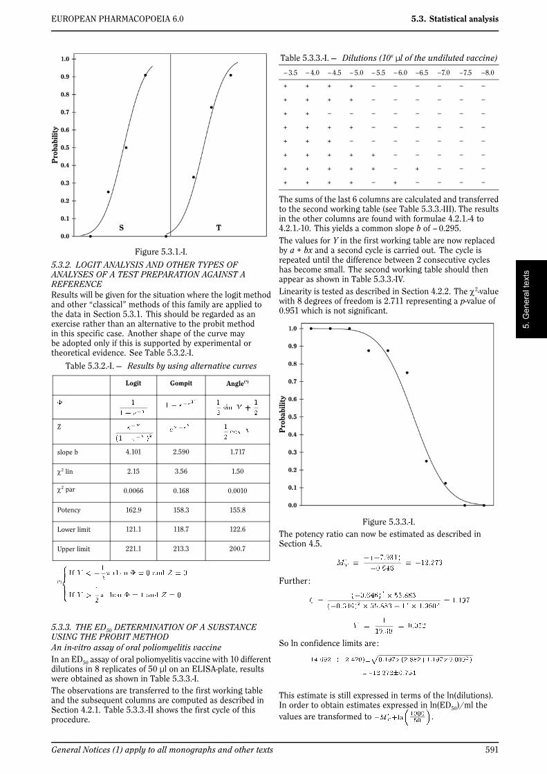
EUROPEAN PHARMACOPOEIA 6.0 5.3. Statistical analysis
Figure 5.3.1.-I.
5.3.2. LOGIT ANALYSIS AND OTHER TYPES OFANALYSES OF A TEST PREPARATION AGAINST AREFERENCEResults will be given for the situation where the logit methodand other “classical” methods of this family are applied tothe data in Section 5.3.1. This should be regarded as anexercise rather than an alternative to the probit methodin this specific case. Another shape of the curve maybe adopted only if this is supported by experimental ortheoretical evidence. See Table 5.3.2.-I.
Table 5.3.2.-I. — Results by using alternative curves
Logit Gompit Angle(*)
Z
slope b 4.101 2.590 1.717
χ2 lin 2.15 3.56 1.50
χ2 par 0.0066 0.168 0.0010
Potency 162.9 158.3 155.8
Lower limit 121.1 118.7 122.6
Upper limit 221.1 213.3 200.7
(*)
5.3.3. THE ED50 DETERMINATION OF A SUBSTANCEUSING THE PROBIT METHODAn in-vitro assay of oral poliomyelitis vaccineIn an ED50 assay of oral poliomyelitis vaccine with 10 differentdilutions in 8 replicates of 50 µl on an ELISA-plate, resultswere obtained as shown in Table 5.3.3.-I.The observations are transferred to the first working tableand the subsequent columns are computed as described inSection 4.2.1. Table 5.3.3.-II shows the first cycle of thisprocedure.
Table 5.3.3.-I. — Dilutions (10x µl of the undiluted vaccine)
−3.5 −4.0 −4.5 −5.0 −5.5 −6.0 −6.5 −7.0 −7.5 −8.0
+ + + + − − − − − −
+ + + + − − − − − −
+ + − − − − − − − −
+ + + + − − − − − −
+ + + − − − − − − −
+ + + + + − − − − −
+ + + + + − + − − −
+ + + + − + − − − −
The sums of the last 6 columns are calculated and transferredto the second working table (see Table 5.3.3.-III). The resultsin the other columns are found with formulae 4.2.1.-4 to4.2.1.-10. This yields a common slope b of −0.295.The values for Y in the first working table are now replacedby a + bx and a second cycle is carried out. The cycle isrepeated until the difference between 2 consecutive cycleshas become small. The second working table should thenappear as shown in Table 5.3.3.-IV.Linearity is tested as described in Section 4.2.2. The χ2-valuewith 8 degrees of freedom is 2.711 representing a p-value of0.951 which is not significant.
Figure 5.3.3.-I.The potency ratio can now be estimated as described inSection 4.5.
Further :
So ln confidence limits are :
This estimate is still expressed in terms of the ln(dilutions).In order to obtain estimates expressed in ln(ED50)/ml thevalues are transformed to .
General Notices (1) apply to all monographs and other texts 591

5.3. Statistical analysis EUROPEAN PHARMACOPOEIA 6.0
Table 5.3.3.-II. — First working table in the first cycleVaccine Dose n r x p Y Z y w wx wy wx2 wy2 wxy
T 10−3.5 8 0 −8.06 0.000 0.00 0.5 0.399 −1.253 5.09 −41.04 −6.38 330.8 8.00 51.4
10−4.0 8 0 −9.21 0.000 0.00 0.5 0.399 −1.253 5.09 −46.91 −6.38 432.0 8.00 58.8
10−4.5 8 1 −10.36 0.125 0.00 0.5 0.399 −0.940 5.09 −52.77 −4.79 546.8 4.50 49.6
10−5.0 8 2 −11.51 0.250 0.00 0.5 0.399 −0.627 5.09 −58.63 −3.19 675.1 2.00 36.7
10−5.5 8 6 −12.66 0.750 0.00 0.5 0.399 0.627 5.09 −64.50 3.19 816.8 2.00 −40.4
10−6.0 8 7 −13.82 0.875 0.00 0.5 0.399 0.940 5.09 −70.36 4.79 972.1 4.50 −66.1
10−6.5 8 7 −14.97 0.875 0.00 0.5 0.399 0.940 5.09 −76.23 4.79 1140.8 4.50 −71.7
10−7.0 8 8 −16.12 1.000 0.00 0.5 0.399 1.253 5.09 −82.09 6.38 1323.1 8.00 −102.9
10−7.5 8 8 −17.27 1.000 0.00 0.5 0.399 1.253 5.09 −87.95 6.38 1518.9 8.00 −110.2
10−8.0 8 8 −18.42 1.000 0.00 0.5 0.399 1.253 5.09 −93.82 6.38 1728.2 8.00 −117.6
Table 5.3.3.-III. — Second working table in the first cycleVaccine w wx wy wx2 wy2 wxy Sxx Sxy Syy
a
T 50.93 −674.3 11.17 9484.6 57.50 −312.32 556.92 −164.43 55.05 −13.24 0.219 −3.690
Table 5.3.3.-IV. — Second working table after sufficient cyclesVaccine w wx wy wx2 wy2 wxy Sxx Sxy Syy
a
T 19.39 −238.2 0.11 2981.1 26.05 −37.45 55.88 −36.11 26.05 −12.28 0.006 −7.931
Since it has become common use to express the potency ofthis type of vaccine in terms of log10(ED50)/ml, the resultshave to be divided by ln(10). The potency is thus estimatedas 6.63 log10(ED50)/ml with 95 per cent confidence limitsfrom 6.30 to 6.96 log10(ED50)/ml.
5.4. EXTENDED SIGMOID DOSE-RESPONSE CURVES5.4.1. FOUR-PARAMETER LOGISTIC CURVE ANALYSISA serological assay of tetanus seraAs already stated in Section 3.4, this example is intended toillustrate a “possible” way to analyse the data presented, butnot necessarily to reflect the “only” or the “most appropriate”way. Many other approaches can be found in the literature,but in most cases they should not yield dramatically differentoutcomes. A short discussion of alternative approaches andother statistical considerations is given in Section 7.5.A guinea-pig antiserum is assayed against a standard serum(0.4 IU/ml) using an enzyme-linked immunosorbent assaytechnique (ELISA). 10 two-fold dilutions of each serum wereapplied on a 96-well ELISA plate. Each dilution was appliedtwice. The observed responses are listed in Table 5.4.1.-I.
Table 5.4.1.-I. — Observed responses
Standard S Preparation to be examined T
Dil. Obs. 1 Obs. 2 Dil. Obs. 1 Obs. 2
1/10 2.912 2.917 1/10 3.017 2.987
1/20 2.579 2.654 1/20 2.801 2.808
1/40 2.130 2.212 1/40 2.401 2.450
1/80 1.651 1.638 1/80 1.918 1.963
1/160 1.073 0.973 1/160 1.364 1.299
1/320 0.585 0.666 1/320 0.861 0.854
1/640 0.463 0.356 1/640 0.497 0.496
1/1280 0.266 0.234 1/1280 0.340 0.344
1/2560 0.228 0.197 1/2560 0.242 0.217
1/5120 0.176 0.215 1/5120 0.178 0.125
For this example, it will be assumed that the laboratoryhas validated conditions 1 to 3 in Section 3.1.1 when theassay was being developed for routine use. In addition, thelaboratory has validated that the upper limit and lower limitof the samples can be assumed to be equal.
No unusual features are discovered in a graphicalrepresentation. A least squares method of a suitablecomputer program is used to fit the parameters of thelogistic function, assuming that the residual error termsare independent and identically distributed normal randomvariables. In this case, 3 parameters (α, β and δ) are neededto describe the common slope-factor and the common lowerand upper asymptotes. 2 additional parameters (γS and γT) areneeded to describe the horizontal location of the 2 curves.
The following estimates of the parameters are returned bythe program:
In addition, the estimated residual variance (s2) is returnedas 0.001429 with 20 degrees of freedom (within-treatmentsvariation).
In order to obtain confidence limits, and also to checkfor parallelism and linearity, the observed responses (u)are linearised and submitted to a weighted parallel-lineanalysis by the program. This procedure is very similar tothat described in Section 4.2 for probit analysis with thefollowing modifications :
592 See the information section on general monographs (cover pages)

EUROPEAN PHARMACOPOEIA 6.0 5.3. Statistical analysis
The resulting weighted analysis of variance of thetransformed responses (y) using weights (w) is shown inTable 5.4.1.-II.
Table 5.4.1.-II — Weighted analysis of variance
Source of variation Degrees offreedom Chi-square Probability
Preparations 1 0.529653 0.467
Regression 1 6599.51 0.000
Non-parallelism 1 0.0458738 0.830
Non-linearity 16 8.89337 0.918
Treatments 19 6608.98 0.000
Residual error 20 20.0000
Total 39 6628.98
There are no significant deviations from parallelism andlinearity and thus the assay is satisfactory for potencycalculations. If the condition of equal upper and lowerasymptotes is not fulfilled, significant deviations fromlinearity and/or parallelism are likely to occur because thetests for linearity and parallelism reflect the goodness of fitof the complete four-parameter model. The residual error inthe analysis of variance is always equal to 1 as a result of thetransformation. However, a heterogeneity factor (analogousto that for the probit model) can be computed.
The relative potency of the test preparation can beobtained as the antilogarithm of γS − γT. Multiplying bythe assigned potency of the standard yields an estimate of1.459 × 0.4 = 0.584 IU/ml. Formula 4.2.3.-2 gives 95 percent confidence limits from 0.557-0.612 IU/ml.
6. COMBINATION OF ASSAY RESULTS
6.1. INTRODUCTION
Replication of independent assays and combination of theirresults is often needed to fulfil the requirements of theEuropean Pharmacopoeia. The question then arises as towhether it is appropriate to combine the results of suchassays and if so in what way.
2 assays may be regarded as mutually independent whenthe execution of either does not affect the probabilities ofthe possible outcomes of the other. This implies that therandom errors in all essential factors influencing the result(for example, dilutions of the standard and of the preparationto be examined, the sensitivity of the biological indicator) inone assay must be independent of the corresponding randomerrors in the other one. Assays on successive days using theoriginal and retained dilutions of the standard therefore arenot independent assays.
There are several methods for combining the results ofindependent assays, the most theoretically acceptable beingthe most difficult to apply. 3 simple, approximate methodsare described below; others may be used provided thenecessary conditions are fulfilled.
Before potencies from assays based on the parallel-lineor probit model are combined they must be expressed inlogarithms; potencies derived from assays based on theslope-ratio model are used as such. As the former models aremore common than those based on the slope-ratio model, thesymbol M denoting ln potency is used in the formulae in thissection ; by reading R (slope-ratio) for M, the analyst may use
the same formulae for potencies derived from assays basedon the slope-ratio model. All estimates of potency must becorrected for the potency assigned to each preparation to beexamined before they are combined.
6.2. WEIGHTED COMBINATION OF ASSAY RESULTS
This method can be used provided the following conditionsare fulfilled :
1) the potency estimates are derived from independentassays ;
2) for each assay C is close to 1 (say less than 1.1) ;
3) the number of degrees of freedom of the individualresidual errors is not smaller than 6, but preferably largerthan 15;
4) the individual potency estimates form a homogeneousset (see Section 6.2.2).
When these conditions are not fulfilled this method cannotbe applied. The method described in Section 6.3 may thenbe used to obtain the best estimate of the mean potency tobe adopted in further assays as an assumed potency.
6.2.1. CALCULATION OF WEIGHTING COEFFICIENTSIt is assumed that the results of each of the n′ assayshave been analysed to give n′ values of M with associatedconfidence limits. For each assay the logarithmic confidenceinterval L is obtained by subtracting the lower limit from theupper. A weight W for each value of M is calculated fromequation 6.2.1.-1, where t has the same value as that used inthe calculation of confidence limits.
(6.2.1.-1)
6.2.2. HOMOGENEITY OF POTENCY ESTIMATESBy squaring the deviation of each value of M from theweighted mean, multiplying by the appropriate weight andsumming over all assays, a statistic is obtained which isapproximately distributed as χ2 (see Table 8.3) and whichmay be used to test the homogeneity of a set of ln potencyestimates :
(6.2.2.-1)
If the calculated χ2 is smaller than the tabulated valuecorresponding to (n′ − 1) degrees of freedom the potenciesare homogeneous and the mean potency and limits obtainedin Section 6.2.3 will be meaningful.
If the calculated value of this statistic is greater than thetabulated value, the potencies are heterogeneous. Thismeans that the variation between individual estimates of M isgreater than would have been predicted from the estimates ofthe confidence limits, i.e. that there is a significant variabilitybetween the assays. Under these circumstances condition 4is not fulfilled and the equations in Section 6.2.3 are nolonger applicable. Instead, the formulae in Section 6.2.4may be used.
6.2.3. CALCULATION OF THE WEIGHTED MEAN ANDCONFIDENCE LIMITSThe products WM are formed for each assay and their sumdivided by the total weight for all assays to give the logarithmof the weighted mean potency.
(6.2.3.-1)
General Notices (1) apply to all monographs and other texts 593

5.3. Statistical analysis EUROPEAN PHARMACOPOEIA 6.0
The standard error of the ln (mean potency) is taken to bethe square root of the reciprocal of the total weight :
(6.2.3.-2)
and approximate confidence limits are obtained from theantilogarithms of the value given by
(6.2.3.-3)
where the number of degrees of freedom of t equals the sumof the number of degrees of freedom for the error meansquares in the individual assays.
6.2.4. WEIGHTED MEAN AND CONFIDENCE LIMITSBASED ON THE INTRA- AND INTER-ASSAY VARIATIONWhen results of several repeated assays are combined, the(χ2-value may be significant. The observed variation is thenconsidered to have two components :
— the intra-assay variation ,
— the inter-assay variation
where is the unweighted mean. The former varies fromassay to assay whereas the latter is common to all M.
For each M a weighting coefficient is then calculated as :
which replaces W in Section 6.2.3. where t is taken to beapproximately 2.
6.3. UNWEIGHTED COMBINATION OF ASSAY RESULTS
To combine the n′ estimates of M from n′ assays in thesimplest way, the mean is calculated and an estimate of itsstandard deviation is obtained by calculating :
(6.3.-1)
and the limits are :
(6.3.-2)
where t has (n′ − 1) degrees of freedom. The number n′ ofestimates of M is usually small, and hence the value of t isquite large.
6.4. EXAMPLE OF A WEIGHTED MEAN POTENCY WITHCONFIDENCE LIMITS
Table 6.4.-I lists 6 independent potency estimates of thesame preparation together with their 95 per cent confidencelimits and the number of degrees of freedom of their errorvariances. Conditions 1, 2 and 3 in Section 6.2. are met. Theln potencies and the weights are calculated as described inSection 6.2.
Table 6.4.-I. — Potency estimates and confidence intervalsof 6 independent assays
Potencyestimate(I.U./vial)
Lowerlimit
(I.U./vial)
Upperlimit
(I.U./vial)
Degreesof
free-dom
lnpoten-cyM
WeightW
18 367 17 755 19 002 20 9.8183 3777.7
18 003 17 415 18 610 20 9.7983 3951.5
18 064 17 319 18 838 20 9.8017 2462.5
17 832 17 253 18 429 20 9.7887 4003.0
18 635 17 959 19 339 20 9.8328 3175.6
18 269 17 722 18 834 20 9.8130 4699.5
Homogeneity of potency estimates is assessed with formula6.2.2.-1 which gives a χ2 of 4.42 with 5 degrees of freedom.This is not significant (p = 0.49) and thus all conditions aremet.A weighted mean potency is calculated with formula 6.2.3.-1which yields 9.8085.Formula 6.2.3.-2 gives a standard deviation of 0.00673 andapproximate 95 per cent confidence limits of 9.7951 and9.8218 are calculated with formula 6.2.3.-3 where t has120 degrees of freedom.By taking the antilogarithms a potency of 18 187 IU/vialis found with 95 per cent confidence limits from17 946-18 431 IU/vial.
7. BEYOND THIS ANNEXIt is impossible to give a comprehensive treatise ofstatistical methods in a pharmacopoeial text. However, themethods described in this annex should suffice for mostpharmacopoeial purposes. This section tries to give a moreabstract survey of alternative or more general methods thathave been developed. The interested reader is encouraged tofurther explore the existing literature in this area. The useof more specialised statistical methods should, in any case,be left to qualified personnel.
7.1. GENERAL LINEAR MODELSThe methods given in this annex can be described in termsof general linear models (or generalised linear models toinclude the probit and logit methods). The principle is todefine a linear structure matrix X (or design matrix) in whicheach row represents an observation and each column a lineareffect (preparation, block, column, dose). For example : theLatin square design in example 5.1.2 would involve a matrixwith 36 rows and 13 columns. 1 column for each of thepreparations, 1 column for the doses, 5 columns for eachblock except the first, and 5 columns for each row except thefirst. All columns, except the one for doses, are filled with 0or 1 depending on whether or not the observation relatesto the effect. A vector Y is filled with the (transformed)observations. The effects are estimated with the formula(XtX)−1XtY from which the potency estimate m can easily bederived as a ratio of relevant effects. Confidence intervalsare calculated from Fieller’s theorem:
mL, mU
where g
594 See the information section on general monographs (cover pages)

EUROPEAN PHARMACOPOEIA 6.0 5.3. Statistical analysis
and v11, v22, v12 represent the variance multipliers for thenumerator, the denominator and their covariance multiplierrespectively. These are taken directly from (XtX)−1 orindirectly by noting that :
Var(a1 − a2) = Var(a1) + Var(a2)–2Cov(a1,a2)
and Cov(a1 − a2 ,b) = Cov(a1 ,b) − Cov(a2 ,b)
A full analysis of variance in which all components arepartitioned is slightly more complicated as it involves arenewed definition of X with more columns to relax theassumptions of parallelism and linearity, after which thelinear hypotheses can be tested. For assays depending uponquantal responses the linear effects (intercepts aS, aT etc. andthe common slope b are found by maximising the sum overtreatments of nln (ai + bx) + (n − r)ln(1 − (ai + bx)) wherex is the ln(dose), denotes the shape of the distributionand i ∈ {S, T, ...}.
7.2. HETEROGENEITY OF VARIANCE
Heterogeneity of variance cannot always be solved by simplytransforming the responses. A possible way to cope withthis problem is to perform a weighted linear regression.In order to obtain an unbiased estimate, the weight of theobservations is taken to be proportional to the reciprocalof the error variances. Since the true error variance is notalways known, an iterative reweighted linear procedure maybe followed. However, the calculation of the confidenceinterval involves new problems.
7.3. OUTLIERS AND ROBUST METHODS
The method of least squares described in this annex hasthe disadvantage of being very sensitive to outliers. Aclear outlier may completely corrupt the calculations. Thisproblem is often remedied by discarding the outlying resultfrom the dataset. This policy can lead to arbitrary rejectionof data and is not always without danger. It is not easy togive a general guideline on how to decide whether or not aspecific observation is an outlier and it is for this reason thatmany robust methods have been developed. These methodsare less sensitive to outliers because they give less weight toobservations that are far away from the predicted value. Newproblems usually arise in computing confidence intervals ordefining a satisfactory function to be minimised.
7.4. CORRELATED ERRORS
Absolute randomisation is not always feasible or veryundesirable from a practical point of view. Thus, subsequentdoses within a dilution series often exhibit correlated errorsleading to confidence limits that are far too narrow. Somemethods have been developed that take account of thisautocorrelation effect.
7.5. EXTENDED NON-LINEAR DOSE-RESPONSE CURVES
Analysis of extended non-linear dose-response curves raises anumber of statistical questions which require consideration,and for which professional advice is recommended. Someof these are indicated below.
1) An example using the four-parameter logistic function hasbeen shown. However, models based on functions givingother sigmoid curves may also be used. Models incorporatingadditional asymmetry parameters have been suggested.
2) Heterogeneity of variance is common when responsescover a wide range. If the analysis ignores the heterogeneity,interpretation of results may not be correct and estimatesmay be biased. Use of the reciprocal of the error variances
as weights is unlikely to be reliable with limited numbersof replicates. It may be appropriate to estimate a functionwhich relates variance to mean response.3) The statistical curve-fitting procedures may give differentestimates depending on assumptions made about thehomogeneity of the variance and on the range of responsesused.4) In principle, equality of upper and lower response limitsfor the different preparations included in an assay can bedirectly tested in each assay. However, interpretation of theresults of these tests may not be straightforward. The testsfor linearity and parallelism given by the simplified methodof analysis (Example 5.4.1) indirectly incorporate tests forequality and accuracy of upper and lower limits.5) Many assays include “controls” which are intended toidentify the upper and/or lower response limits. However,these values may not be consistent with the statisticallyfitted upper and lower response limits based on the extendeddose-response curve.6) The simplified method of analysis given in Example 5.4.1provides approximate confidence intervals. Other methodsmay also be used, for example intervals based on lack-of-fit ofthe completely specified model. For typical assay data, withresponses covering the complete range for each preparationtested, all methods give similar results.
7.6. NON-PARALLELISM OF DOSE-RESPONSE CURVESSimilarity of dose-response relationships is a fundamentalcriterion for assessing whether an assay may be regardedas a dilution assay and hence whether the estimation ofrelative potency is valid (see Section 3.1.1). This criterionis frequently met by showing that dose-response curves forstandard and test samples do not deviate significantly fromparallelism. Underestimation of the residual error can leadto excess rejection of assays due to significant deviationsfrom parallelism and/or linearity. This is often an artefact ofinappropriate assay design or analysis. Minor modificationsto assay designs might in many cases substantially improvethe estimation of the residual error. Analysis allowing forthe actual level of replication may also improve the situation.If estimation of the relevant residual error is not feasiblefor individual assays, for example because it is impracticalto create independent doses and/or replicates, it might bepossible to obtain a more correct estimate of the residualerror during the assay validation process. There may alsobe cases where the assay system is sufficiently precise todetect slight but genuine non-parallelism. If there is truenon-parallelism this needs to be recognised and a suitablesolution adopted. A solution might, for example, requirea suitable standard that is similar in composition to, andtherefore parallel to, the test samples. If the assay systemis responding in a non-specific manner to extraneouscomponents of the standard or test samples, then a morespecific assay system that does not respond to the irrelevantcomponents may be the solution. No simple, generallyapplicable statistical solution exists to overcome thesefundamental problems. The appropriate action has to bedecided on a case-by-case basis with the help of statisticalexpertise.
8. TABLES AND GENERATINGPROCEDURESThe tables in this section list the critical values for the mostfrequently occurring numbers of degrees of freedom. Ifa critical value is not listed, reference should be made tomore extensive tables. Many computer programs includestatistical functions and their use is recommended instead
General Notices (1) apply to all monographs and other texts 595

5.3. Statistical analysis EUROPEAN PHARMACOPOEIA 6.0
of the tables in this section. Alternatively, the generatingprocedures given below each table can be used to computethe probability corresponding to a given statistic and numberof degrees of freedom.
8.1. THE F-DISTRIBUTIONIf an observed value is higher than the value in Table 8.1.-I,it is considered to be significant (upper lines, p = 0.05) orhighly significant (lower lines, p = 0.01). df1 is the number ofdegrees of freedom of the numerator and df2 is the numberof degrees of freedom of the denominator.
Generating procedure. Let F be the F-ratio and df1 anddf2 as described above. Let pi = = 3.14159265358979...The procedure in Table 8.1.-II will then generate the p-value.
8.2. THE -DISTRIBUTION
If an observed value is higher than the value in Table 8.2.-I, itis considered to be significant (p = 0.05) or highly significant(p = 0.01).
Generating procedures. The p-value for a given t with dfdegrees of freedom can be found with the procedures inSection 8.1 where F = t2, df1 = 1 and df2 = df.
Table 8.1.-I — Critical values of the F-distributiondf1 → 1 2 3 4 5 6 8 10 12 15 20 ∞
df2 ↓
10 4.965 4.103 3.708 3.478 3.326 3.217 3.072 2.978 2.913 2.845 2.774 2.538
10.044 7.559 6.552 5.994 5.636 5.386 5.057 4.849 4.706 4.558 4.405 3.909
12 4.747 3.885 3.490 3.259 3.106 2.996 2.849 2.753 2.687 2.617 2.544 2.296
9.330 6.927 5.953 5.412 5.064 4.821 4.499 4.296 4.155 4.010 3.858 3.361
15 4.543 3.682 3.287 3.056 2.901 2.790 2.641 2.544 2.475 2.403 2.328 2.066
8.683 6.359 5.417 4.893 4.556 4.318 4.004 3.805 3.666 3.522 3.372 2.868
20 4.351 3.493 3.098 2.866 2.711 2.599 2.447 2.348 2.278 2.203 2.124 1.843
8.096 5.849 4.938 4.431 4.103 3.871 3.564 3.368 3.231 3.088 2.938 2.421
25 4.242 3.385 2.991 2.759 2.603 2.490 2.337 2.236 2.165 2.089 2.007 1.711
7.770 5.568 4.675 4.177 3.855 3.627 3.324 3.129 2.993 2.850 2.699 2.169
30 4.171 3.316 2.922 2.690 2.534 2.421 2.266 2.165 2.092 2.015 1.932 1.622
7.562 5.390 4.510 4.018 3.699 3.473 3.173 2.979 2.843 2.700 2.549 2.006
50 4.034 3.183 2.790 2.557 2.400 2.286 2.130 2.026 1.952 1.871 1.784 1.438
7.171 5.057 4.199 3.720 3.408 3.186 2.890 2.698 2.563 2.419 2.265 1.683
∞ 3.841 2.996 2.605 2.372 2.214 2.099 1.938 1.831 1.752 1.666 1.571 1.000
6.635 4.605 3.782 3.319 3.017 2.802 2.511 2.321 2.185 2.039 1.878 1.000
Table 8.1.-II — Generating procedure for the F-distributionIf df1 is even If df1 is odd and df2 is even If df1 and df2 are odd
x=df1/(df1+df2/F) x=df2/(df2+df1*F) x=atn(sqr(df1*F/df2))s=1 s=1 cs=cos(x)t=1 t=1 sn=sin(x)for i=2 to (df1-2) step 2 for i=2 to (df2-2) step 2 x=x/2t=t*x*(df2+i-2)/i t=t*x*(df1+i-2)/i s=0s=s+t s=s+t t=sn*cs/2next i next i v=0p=s*(1-x)^(df2/2) p=1-s*(1-x)^(df1/2) w=1
for i=2 to (df2-1) step 2s=s+tt=t*i/(i+1)*cs*csnext ifor i=1 to (df1-2) step 2v=v+ww=w*(df2+i)/(i+2)*sn*snnext ip=1+(t*df2*v-x-s)/pi*4
596 See the information section on general monographs (cover pages)
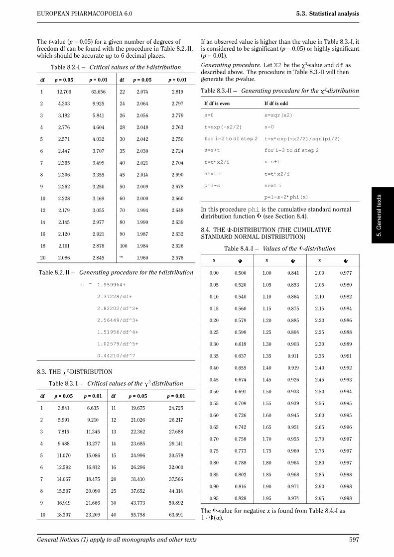
EUROPEAN PHARMACOPOEIA 6.0 5.3. Statistical analysis
The t-value (p = 0.05) for a given number of degrees offreedom df can be found with the procedure in Table 8.2.-II,which should be accurate up to 6 decimal places.
Table 8.2.-I — Critical values of the t-distribution
df p = 0.05 p = 0.01 df p = 0.05 p = 0.01
1 12.706 63.656 22 2.074 2.819
2 4.303 9.925 24 2.064 2.797
3 3.182 5.841 26 2.056 2.779
4 2.776 4.604 28 2.048 2.763
5 2.571 4.032 30 2.042 2.750
6 2.447 3.707 35 2.030 2.724
7 2.365 3.499 40 2.021 2.704
8 2.306 3.355 45 2.014 2.690
9 2.262 3.250 50 2.009 2.678
10 2.228 3.169 60 2.000 2.660
12 2.179 3.055 70 1.994 2.648
14 2.145 2.977 80 1.990 2.639
16 2.120 2.921 90 1.987 2.632
18 2.101 2.878 100 1.984 2.626
20 2.086 2.845 ∞ 1.960 2.576
Table 8.2.-II — Generating procedure for the t-distribution
t = 1.959964+
2.37228/df+
2.82202/df^2+
2.56449/df^3+
1.51956/df^4+
1.02579/df^5+
0.44210/df^7
8.3. THE 2-DISTRIBUTION
Table 8.3.-I — Critical values of the 2-distribution
df p = 0.05 p = 0.01 df p = 0.05 p = 0.01
1 3.841 6.635 11 19.675 24.725
2 5.991 9.210 12 21.026 26.217
3 7.815 11.345 13 22.362 27.688
4 9.488 13.277 14 23.685 29.141
5 11.070 15.086 15 24.996 30.578
6 12.592 16.812 16 26.296 32.000
7 14.067 18.475 20 31.410 37.566
8 15.507 20.090 25 37.652 44.314
9 16.919 21.666 30 43.773 50.892
10 18.307 23.209 40 55.758 63.691
If an observed value is higher than the value in Table 8.3.-I, itis considered to be significant (p = 0.05) or highly significant(p = 0.01).
Generating procedure. Let X2 be the χ2-value and df asdescribed above. The procedure in Table 8.3.-II will thengenerate the p-value.
Table 8.3.-II — Generating procedure for the 2-distribution
If df is even If df is odd
s=0 x=sqr(x2)
t=exp(-x2/2) s=0
for i=2 to df step 2 t=x*exp(-x2/2)/sqr(pi/2)
s=s+t for i=3 to df step 2
t=t*x2/i s=s+t
next i t=t*x2/i
p=1-s next i
p=1-s-2*phi(x)
In this procedure phi is the cumulative standard normaldistribution function (see Section 8.4).
8.4. THE -DISTRIBUTION (THE CUMULATIVESTANDARD NORMAL DISTRIBUTION)
Table 8.4.-I — Values of the -distribution
x x x
0.00 0.500 1.00 0.841 2.00 0.977
0.05 0.520 1.05 0.853 2.05 0.980
0.10 0.540 1.10 0.864 2.10 0.982
0.15 0.560 1.15 0.875 2.15 0.984
0.20 0.579 1.20 0.885 2.20 0.986
0.25 0.599 1.25 0.894 2.25 0.988
0.30 0.618 1.30 0.903 2.30 0.989
0.35 0.637 1.35 0.911 2.35 0.991
0.40 0.655 1.40 0.919 2.40 0.992
0.45 0.674 1.45 0.926 2.45 0.993
0.50 0.691 1.50 0.933 2.50 0.994
0.55 0.709 1.55 0.939 2.55 0.995
0.60 0.726 1.60 0.945 2.60 0.995
0.65 0.742 1.65 0.951 2.65 0.996
0.70 0.758 1.70 0.955 2.70 0.997
0.75 0.773 1.75 0.960 2.75 0.997
0.80 0.788 1.80 0.964 2.80 0.997
0.85 0.802 1.85 0.968 2.85 0.998
0.90 0.816 1.90 0.971 2.90 0.998
0.95 0.829 1.95 0.974 2.95 0.998
The -value for negative x is found from Table 8.4.-I as1 - (-x).
General Notices (1) apply to all monographs and other texts 597

5.3. Statistical analysis EUROPEAN PHARMACOPOEIA 6.0
Generating procedure : Let x be the x-value. The procedurein Table 8.4.-II will generate the corresponding -value if0 ≤ x ≤ 8.15. If x is greater than 8.15 the -value can be setto 1. If x is negative, the formula given above can be used.This procedure assumes that the computer can representabout 15 decimal places. If less digits or more digits can berepresented, the procedure needs some trivial modifications.
Table 8.4.-II — Generating procedure for the -distribution
s=0
t=x
i=1
repeat
s=s+t
i=i+2
t=t*x*x/i
until t<1E-16
phi=0.5+s*exp(-x*x/2)/sqr(2*pi)
8.5. RANDOM PERMUTATIONSRandom permutations are needed in randomised blockdesigns. The following algorithm shows how the built-inrandom generator of a computer can be used to createrandom permutations of N treatments.Step 1. Write the N possible treatments down in a row.Step 2. Obtain a random integer r such that 1≤ r ≤ N.Step 3. Exchange the r-th treatment with the N-th treatmentin the row.Step 4. Let N = N − 1 and repeat steps 2 to 4 until N = 1.
An example with 6 treatments will illustrate this algorithm.
1. N = 6 S1 S2 S3 T1 T2 T3
2. r = 2 → ←
3. S1 T3 S3 T1 T2 S2
4. N = 5
2. r = 4 → ←
3. S1 T3 S3 T2 T1 S2
4. N = 4
2. r = 4 ↓
3. S1 T3 S3 T2 T1 S2
4. N = 3
2. r = 1 → ←
3. S3 T3 S1 T2 T1 S2
4. N = 2
2. r = 1 → ←
3. T3 S3 S1 T2 T1 S2
4. N = 1
8.6. LATIN SQUARESThe following example shows how 3 independentpermutations can be used to obtain a Latin square.1) Generate a random permutation of the N possibletreatments (see Section 8.5) :
T3 S3 S1 T2 T1 S2
2) A simple Latin square can now be constructed by“rotating” this permutation to the right. This can be done asfollows. Write the permutation found in step 1 down on thefirst row. The second row consists of the same permutation,but with all treatments shifted to the right. The rightmosttreatment is put on the empty place at the left. This isrepeated for all the rows until all the treatments appear oncein each column:
T3 S3 S1 T2 T1 S2
S2 T3 S3 S1 T2 T1
T1 S2 T3 S3 S1 T2
T2 T1 S2 T3 S3 S1
S1 T2 T1 S2 T3 S3
S3 S1 T2 T1 S2 T3
3) Generate 2 independent random permutations of thefigures 1 to N :— one for the rows :
2 3 6 1 4 5
— and one for the columns :
3 4 6 2 5 1
4) The Latin square can now be found by sorting the rowsand columns of the simple Latin square according to the2 permutations for the rows and columns :
3 4 6 2 5 1
2 T3 S3 S1 T2 T1 S2
3 S2 T3 S3 S1 T2 T1
6 T1 S2 T3 S3 S1 T2
1 T2 T1 S2 T3 S3 S1
4 S1 T2 T1 S2 T3 S3
5 S3 S1 T2 T1 S2 T3
↓
1 2 3 4 5 6
1 S1 T3 T2 T1 S3 S2
2 S2 T2 T3 S3 T1 S1
3 T1 S1 S2 T3 T2 S3
4 S3 S2 S1 T2 T3 T1
5 T3 T1 S3 S1 S2 T2
6 T2 S3 T1 S2 S1 T3
9. GLOSSARY OF SYMBOLS
Symbol Definition
a Intersection of linear regression ofresponses on dose or ln(dose)
b Slope of linear regression of responses ondose or on ln(dose)
598 See the information section on general monographs (cover pages)

EUROPEAN PHARMACOPOEIA 6.0 5.3. Statistical analysis
Symbol Definition
d Number of dose levels for each preparation(excluding the blank in slope-ratio assays)
e Base of natural logarithms(= 2.71828182845905...)
g Statistic used in Fieller’s theorem:
h Number of preparations in an assay,including the standard preparation
m Potency estimate obtained as a ratio ofeffects in general linear models
n Number of replicates for each treatment
p Probability of a given statistic being largerthan the observed value. Also used as theratio r/n in probit analysis
r The number of responding units pertreatment group in assays depending uponquantal responses
s Estimate of standard deviation ( )
s2 Estimate of residual variance given by errormean square in analysis of variance
t Student’s statistic (Table 8.2.)
u Observed response in four-parameteranalysis
v11,v12,v22 (Co)variance multipliers for numerator anddenominator of ratio m in Fieller’s theorem
w Weighting coefficient
x The ln(dose)
y Individual response or transformedresponse
A Assumed potencies of test preparationswhen making up doses
B Mean response to blanks in slope-ratioassays
C Statistic used in the calculation of
confidence intervals :
C1, ... , Cn Mean response to each column of a Latinsquare design
D1,D2 Mean response on time 1 or time 2 in thetwin cross-over design
F Ratio of 2 independent estimates of variancefollowing an F-distribution (Table 8.1.)
GS,GT, ... Treatment values used in the analysis ofvariance for slope-ratio assays
Symbol Definition
HP, HL Multipliers used in the analysis of variancefor parallel-line assays
HB, HI Multipliers used in the analysis of variancefor slope-ratio assays
I In parallel-line assays, the ln of the ratiobetween adjacent doses. In slope-ratioassays, the interval between adjacent doses
JS, JT, ... Linearity values used in the analysis ofvariance for slope-ratio assays
K Correction term used in the calculation ofsums of squares in the analysis of variance
L Width of confidence interval in logarithms
LS, LT, ... Linear contrasts of standard and testpreparations
M′ ln potency ratio of a given test preparation
N Total number of treatments in theassay (= dh)
PS, PT, ... Sum of standard and test preparations
R Estimated potency of a given testpreparation
R′ Potency ratio of a given test preparation
R1, ... , Rn Mean response in each of rows 1 to n of aLatin square design, or in each block of arandomised block design
S Standard preparation
S1, ... , Sd Mean response to the lowest dose 1 upto the highest dose d of the standardpreparation S
SS Sum of squares due to a given source ofvariation
T, U, V, ... Test preparations
T1, ... , Td Mean response to the lowest dose 1 up tothe highest dose d of test preparation T
V Variance coefficient in the calculation ofconfidence limits
W Weighting factor in combination of assayresults
X Linear structure or design matrix used ingeneral linear models
Y Vector representing the (transformed)responses in general linear models
Z The first derivative of
α Upper asymptote of the ln(dose)-responsecurve in four-parameter analysis
General Notices (1) apply to all monographs and other texts 599

5.3. Statistical analysis EUROPEAN PHARMACOPOEIA 6.0
Symbol Definition
β Slope-factor of the ln(dose)-response curvein four-parameter analysis
γ The ln(dose) giving 50 per cent response inthe four-parameter analysis
δ Lower asymptote of the ln(dose)-responsecurve in four-parameter analysis
3.141592653589793238...
Cumulative standard normal distributionfunction (Table 8.4.)
χ2 Chi-square statistic (Table 8.3.)
10. LITERATUREThis section lists some recommended literature for furtherstudy.Finney, D.J. (1971). Probit Analysis, 3rd Ed. CambridgeUniversity Press, Cambridge.
Nelder, J.A. & Wedderburn, R.W.M. (1972). Generalizedlinear models, Journal of the Royal Statistical Society,Series A 135, 370-384.
DeLean, A., Munson, P.J., and Rodbard, D. (1978).Simultaneous analysis of families of sigmoidal curves :Application to bioassay, radioligand assay, and physiologicaldose-response curves, Am. J. Physiol. 235(2) : E97-E102.
Finney, D.J. (1978). Statistical Method in Biological Assay,3rd Ed. Griffin, London.
Sokal, R.R. & Rohlf, F.R. (1981). Biometry : Principles andPractice of Statistics in Biological Research, 2nd Ed. W.H.Freemann & CO, New York.
Peace, K.E. (1988). Biopharmaceutical Statistics for DrugDevelopment, Marcel Dekker Inc., New York/Basel.
Bowerman, B.L. & O’Connell, R.T. (1990). Linear StatisticalModels an Applied Approach, 2nd Ed. PWS-KENT PublishingCompany, Boston.
Govindarajulu, Z. (2001). Statistical Techniques in Bioassay,2nd revised and enlarged edition, Karger, New York.
600 See the information section on general monographs (cover pages)