Embed Size (px)
Citation preview

5220.0.55.002
Information Paper
Gross State Productusing the Productionapproach GSP(P)
Australia
2007
w w w . a b s . g o v . a u

AUST R A L I A N BUR E A U OF STA T I S T I C S
EMBA R G O : 11 . 30 A M (CAN B E R R A T IME ) FR I 14 SEP 2007
B r i a n P i n k
A u s t r a l i a n S t a t i s t i c i a n
Information Paper
Gross State Productusing the Productionapproach GSP(P)
Australia
2007
NewIssue
! For further information about these and related statistics, contact the NationalInformation and Referral Service on 1300 135 070 or Steve Whennan on Canberra(02) 6252 6711.
I N Q U I R I E S
Produced by the Austra l ian Bureau of Stat ist ics
In all cases the ABS must be acknowledged as the source when reproducing or
quoting any part of an ABS publ icat ion or other product.
This work is copyr ight. Apart from any use as permitted under the Copyright Act
1968 , no part may be reproduced by any process without prior written permission
from the Commonwealth. Requests and inquir ies concerning reproduct ion and rights
in this publ icat ion should be addressed to The Manager, Intermediary Management,
Austra l ian Bureau of Stat ist ics, Locked Bag 10, Belconnen ACT 2616, by telephone
(02) 6252 6998, fax (02) 6252 7102, or email :
© Commonwealth of Austral ia 2007
ISBN 9780642483522
ABS Catalogue No. 5220.0.55.002
CO N T E N T S . . . . . . . . . . . . . . . . . . . . . . . . . . . . . . . . . . . . . . . . . . . .
99Conclusion and Future Directions3 . . . . . . . . . . . . . . . . . . . . . . . . . . . . .22GSP Using the Production Approach – Industry Gross Value Added2 . . . . . . . .1GSP Using the Production Approach – By State1 . . . . . . . . . . . . . . . . . . . . .ixIntroduction . . . . . . . . . . . . . . . . . . . . . . . . . . . . . . . . . . . . . . . . . . . . .viiPreface . . . . . . . . . . . . . . . . . . . . . . . . . . . . . . . . . . . . . . . . . . . . . . . .
page
A B S • GR O S S ST A T E P R O D U C T U S I N G T H E P R O D U C T I O N A P P R O A C H GS P ( P ) • 5 2 2 0 . 0 . 5 5 . 0 0 2 • 2 0 0 7 v


PR E F A C E . . . . . . . . . . . . . . . . . . . . . . . . . . . . . . . . . . . . . . . . . . . . . .
B r i a n P i n k
Au s t r a l i a n S t a t i s t i c i a n
Since 1987 the Australian Bureau of Statistics (ABS) has published annual estimates of
Gross State Product (GSP) as part of the Australian National Accounts: State Accounts
(cat. no. 5220.0). Over recent years there has been an increased effort applied to
improving and expanding the quality of the State Accounts. In 2003, the ABS established
a specialist team with a focus on the State Accounts.
Compiling GSP using the Production approach (GSP(P)) was the major project on the
research program. Another aspect was the establishment of a State Accounts User Group
(SAUG) in 2004. Since 2004 consultation and discussion has taken place with SAUG on
the development of the GSP(P) volume estimates.
This information paper provides the results of the GSP(P) project. Results are presented
for each state followed by a discussion on Gross Value Added (GVA) by industry
(including Ownership of dwellings and Taxes less subsidies on products) for each state.
The GSP(P) estimates are compared to the current official volume estimates of GSP
growth which are based on the Income/Expenditure approach (GSP(I/E)). The GSP(P)
estimates contained in this information paper are considered indicative.
The compilation of the GSP(P) estimates means that there are now alternative measures
of economic activity available for each state. There are three possible volume measures
of GSP that the ABS could publish as the headline measure of economic growth:
! the new GSP(P) based volume estimates
! the current official GSP(I/E) based volume estimates
! an average of these volume estimates, described as GSP(A).
In considering the merits of the various options the ABS, in consultation with the SAUG,
concluded that the average measure is preferred. The ABS considers this measure
maximises the use of information about state economic activity and that it will be more
stable over time (i.e. subject to smaller revisions) than the two alternatives. This
approach is also consistent with the approach used nationally for the latest year
estimates and for the quarterly national accounts.
A B S • GR O S S ST A T E P R O D U C T U S I N G T H E P R O D U C T I O N A P P R O A C H GS P ( P ) • 5 2 2 0 . 0 . 5 5 . 0 0 2 • 2 0 0 7 v i i

AB B R E V I A T I O N S . . . . . . . . . . . . . . . . . . . . . . . . . . . . . . . . . . . . . .
Value of Agricultural Commodities ProducedVACP
System of National Accounts 1993SNA93
System of National AccountsSNA
State Accounts User GroupSAUG
Quarterly Business Indicators SurveyQBIS
producer price indexPPI
National Electricity Market Management Company LimitedNEMMCO
National Centre for Vocational Education ResearchNCVER
household final consumption expenditureHFCE
gross value addedGVA
goods and services taxGST
income approach to measuring GSPGSP(I)
production approach to measuring GSPGSP (P)
income/expenditure approach to measuring GSPGSP (I/E)
expenditure approach to measuring GSPGSP (E)
average of GSP measuresGSP (A)
gross state productGSP
Government Finance StatisticsGFS
government final consumption expenditureGFCE
gross domestic productGDP
Australian Government Department of Industry, Tourism and ResourcesDITR
Australian Government Department of Education, Science and TrainingDEST
consumer price indexCPI
Bureau of Transport and Regional EconomicsBTRE
Building Activity SurveyBACS
Australian System of National AccountsASNA
Australian Prudential Regulation AuthorityAPRA
Australian and New Zealand Standard Industrial ClassificationANZSIC
Australian Bureau of StatisticsABS
Australian Bureau of Agricultural and Resource EconomicsABARE
v i i i A B S • GR O S S ST A T E P R O D U C T U S I N G T H E P R O D U C T I O N A P P R O A C H GS P ( P ) • 5 2 2 0 . 0 . 5 5 . 0 0 2 • 2 0 0 7

IN T R O D U C T I O N . . . . . . . . . . . . . . . . . . . . . . . . . . . . . . . . . . . . . . .
The introduction of GSP(P) estimates means that there are now alternative measures of
economic activity available for each state. There are three possible volume measures of
GSP that the ABS could publish as headline measure of economic growth:
! the new GSP(P) based volume estimates
! the current official GSP(I/E) based volume estimates
! a simple average of these volume estimates, described here as GSP(A).
In considering the merits of the various options the ABS, in consultation with SAUG,
concluded that the average measure is preferred. The ABS considers this measure
maximises the use of information about state economic activity and that it will be more
stable over time (i.e. subject to smaller revisions) than the two alternatives. This
approach is also consistent with the approach used nationally for the latest year
estimates and for the quarterly national accounts.
HE A D L I N E ME A S U R E S OF
GS P
The ABS has published estimates of GSP as part of the Australian National Accounts:
State Accounts (cat. no. 5220.0) on a regular basis since 1987. Since this time there has
been ongoing work to improve the estimates of GSP and expand the amount of
information contained within the State Accounts. The main improvements to the State
Accounts include:
! 1988–89 – introduction of Market Prices
! 1991–92 – introduction of State Final Demand
! 1993–94 – constant price estimates introduced using prices at 1989–90 and Industry
structure changed to the Australian and New Zealand Industrial Classification,
1993 (ANZSIC93) (cat. no. 1292.0.15.001) basis
! 1997–98 – implementation of accounts based on the System of National Accounts,
1993 (SNA93) from 1989–90 onwards and change from constant price estimates to
chain volume measure estimates.
Over recent years there has been an increased effort applied to improving and expanding
the quality of the State Accounts. In 2003, the ABS allocated additional resources to
establish a specialist team with a focus on the State Accounts. Investigating the possibility
of compiling GSP(P) was the major project on the research program. Another aspect was
the establishment of a SAUG in 2004. Since 2004 consultation and discussion has taken
place with the SAUG on the development of the GSP(P) volume estimates.
This information paper provides the results of the GSP(P) project. Results for each state
are presented, followed by a discussion on GVA by industry (including Ownership of
dwellings and Taxes less subsidies on products) for each state. Comparisons of GSP(P)
are made to the current official volume estimate of GSP growth which are based on
GSP(I/E). The GSP(I/E) volume estimates are derived by deflating current price GSP
compiled using the income approach (GSP(I)), with a deflator compiled using the
expenditure approach (GSP(E)).
I N T R O D U C T I O N
A B S • GR O S S ST A T E P R O D U C T U S I N G T H E P R O D U C T I O N A P P R O A C H GS P ( P ) • 5 2 2 0 . 0 . 5 5 . 0 0 2 • 2 0 0 7 i x

The remainder of the paper is structured as follows:
! Section 1 outlines the methodologies used to derive GVA at the Australia level
compared with the states and territories, and a comparison of the various GSP
measures. It includes a comparison of the levels and growth rates of the three
measures of GSP (GSP(P), GSP(I/E) and GSP(A)) and other additional analysis for
each state/territory.
ST R U C T U R E OF PA P E R
The GSP(I/E) estimates shown in this paper are those published in the 2005–06 issue of
Australian National Accounts: State Accounts, which are the most recent official
estimates. It is expected that these estimates will be revised in the 2006–07 issue of
5220.0 primarily due to updated Australia level benchmarks from the annual supply and
use tables and the availability of additional data sources.
The GSP(P) and GSP(A) estimates shown in this paper should be regarded as indicative.
They are not official ABS estimates. Their purpose is to demonstrate the GSP(P)
approach. While the ABS has taken care in developing these estimates, they are likely to
be revised in the 2006–07 issue of 5220.0, at which stage they will become official
estimates.
ST A T U S OF TH E
ES T I M A T E S IN TH I S
PA P E R
The GSP(I/E) estimates have been regarded as experimental estimates since their
inception due to issues relating to the measurement of Interstate trade and Changes in
inventories. The development of GSP(P) has allowed an assessment of the current price
GSP(I) results. Both the volume GSP(P) and volume GSP(I/E) generate similar outcomes.
Consequently the ABS considers the volume estimates to be sufficiently robust, enabling
the experimental status be dropped. The robustness of the estimates is also reinforced
by the use of GSP(A) as the headline measure. Thus, from the 2006–07 publication of
Australian National Accounts: State Accounts, the headline GSP volume estimates will
no longer be labelled as experimental.
Nevertheless, users should be aware that the State Accounts estimates are likely to be of
lower quality than the equivalent national level estimates. One reason is the inherent
problems associated with the allocation of multi-State activities, especially in industries
such as long distance transport, communication and finance. Another reason is the data
sources are generally sample surveys designed to optimise quality at the national level,
not the state level. This is likely to impact more on the quality of data for the smaller
states and territories.
EX P E R I M E N T A L ST A T U S
OF ES T I M A T E S
It is planned to publish GSP(A) as the headline measure in the Australian National
Accounts: State Accounts, 2006–07 for the period from 1989–90 onwards. The volume
estimates published on the GSP(I/E) and GSP(P) bases would, therefore, contain
statistical discrepancies to reconcile them with GSP(A).
The development of the volume estimates of GSP(P) will also have an impact on the
presentation of the current prices estimate of GSP. The volume measure of GSP(P) will
be reflated using the GSP(E) deflator to produce a current price GSP(P). This will then
be used with the existing current price GSP to calculate a simple average of GSP,
estimated using the income approach, in current prices. This is will result in a statistical
discrepancy for the individual measures of current price GSP.
HE A D L I N E ME A S U R E S OF
GS P continued
x A B S • GR O S S ST A T E P R O D U C T U S I N G T H E P R O D U C T I O N A P P R O A C H GS P ( P ) • 5 2 2 0 . 0 . 5 5 . 0 0 2 • 2 0 0 7
I N T R O D U C T I O N
! Section 2 presents a discussion of the structure of the industries under ANZSIC93
and a detailed description of methods and results for each industry.
! Section 3 contains some concluding remarks and outlines changes to the format of
the 2006–07 publication of Australian National Accounts: State Accounts. Areas
requiring further research and development are also presented.
The inclusion of the GSP(A) and GSP(P) estimates is a major change in State Accounts
and, as such, the ABS would be interested in receiving any feedback on these estimates
and their inclusion in Australian National Accounts: State Accounts. Please contact
Donna Grcman (email [email protected] or telephone (02) 6252 5892) if you
have any comments or inquires about the proposed approach.
ST R U C T U R E OF PA P E R
continued
A B S • GR O S S ST A T E P R O D U C T U S I N G T H E P R O D U C T I O N A P P R O A C H GS P ( P ) • 5 2 2 0 . 0 . 5 5 . 0 0 2 • 2 0 0 7 x i
I N T R O D U C T I O N


SECT I O N 1 GS P US I N G TH E PR O D U C T I O N AP P R O A C H – BYST A T E . . . . . . . . . . . . . . . . . . . . . . . . . . . . . . . . . . . . . . . . . . . . . . . . .
The same methods currently used to derive Australian level annual volume estimates of
industry GVA have been used, where possible, in developing the GSP(P) approach.
There are two reasons for this choice. First, the cost of developing and maintaining the
data set required for double deflation based estimates by state is prohibitive. Second, it is
considered that, even if state output and input data by industry were available, these data
would almost certainly be of lower quality than the corresponding national data. Hence
deriving GVA as their difference would be likely to produce unsatisfactory results due to
the compounding of errors in the double deflation approach.
Assumptions have been made, or alternate indicators have been used, on occasions
where data availability has limited the application of the national quarterly method.
The following diagram provides a brief overview of the general methodology for the
GSP(P) estimates.
Methods for State volume
estimates
The annual Australia level volume estimates of GVA for each industry (except for the
latest year) are derived in the annual supply and use tables using double deflation, i.e. by
subtracting volume estimates of intermediate input from volume estimates of output.
Due to data constraints this approach cannot be applied for the latest year (or on a
quarterly basis) except for the Agriculture subdivision.
The quarterly and latest year annual volume estimates of industry GVA for Australia are
derived by using different indicators for each industry to interpolate and extrapolate the
supply use benchmark estimates. Most of the indicators are output indicators. These are
based on either sales data deflated by a suitable price index to obtain sales volumes, or
on physical quantities produced. The method involves extrapolating reference year
estimates of current price GVA using movements in a volume indicator of output. One
exception to the use of output or input indicators is the Agriculture sub-division within
the Agriculture, forestry and fishing industry where a double deflation approach is used.
For more information about the Australia level methodology, please refer to Australian
System of National Accounts, Concepts: Source and Methods (cat. no. 5216.0), Chapters
12 and 24.
Methods for Austral ia
volume est imates
This section presents the general methodology used to estimate GSP(P) and the results
for each state. A brief description of the methodology used for the Australian estimates
which are published in Australian System of National Accounts (ASNA) (cat. no. 5204.0)
is also provided. The state methodology is then presented, followed by a comparison of
the three GSP measures across all states and a more detailed examination of each state's
estimates.
I N T R O D U C T I O N
A B S • GR O S S ST A T E P R O D U C T U S I N G T H E P R O D U C T I O N A P P R O A C H GS P ( P ) • 5 2 2 0 . 0 . 5 5 . 0 0 2 • 2 0 0 7 1

For most industries there are no separate estimates of state current price GVA available.
These estimates are only available on a national basis. The method used to derive a
current price GVA by state for each industry is to split that particular industry GVA to the
states using the factor income shares (compensation of employees, gross operating
surplus and gross mixed income) as currently published in Australian National
Accounts: State Accounts (cat. no. 5220.0).
In order to align with the total national industry factor income estimates published in
table 57 of the Australian System of National Accounts, the General Government Gross
operating surplus by state in tables 24 to 31 in the Australian National Accounts, State
Accounts has been re-allocated to all industries using public employment data by
industry by state from the ABS Employee Earnings and Hours, Australia
(cat. no. 6306.0).
Australia GVA by Industry in current prices
Allocate to states using factor income shares
State GVA by Industry in current prices
Apply quantity revaluation or price deflation
Use output indicator with price information
State GVA by Industry
to create the output indicator
to create chain volume measure
Flowchart of GSP(P) compilation methodology
Ownership of dwellings
GSP(P)
and Taxes less subsidies on products
chain volume measures
Methods for State volume
estimates cont inued
2 A B S • GR O S S ST A T E P R O D U C T U S I N G T H E P R O D U C T I O N A P P R O A C H GS P ( P ) • 5 2 2 0 . 0 . 5 5 . 0 0 2 • 2 0 0 7
SE C T I O N 1 • G S P U S I N G T H E P R O D U C T I O N A P P R O A C H – B Y S T A T E

Currently the ABS compiles two different measures of GSP, GSP(I) which uses the
income approach and GSP(E) which uses the expenditure approach. Both measures are
currently published in Australian National Accounts: State Accounts.
GSP(I) is calculated for each state by adding compensation of employees, gross
operating surplus, gross mixed income, taxes less subsidies on production and imports,
and the Australian statistical discrepancy.
GSP(E) is calculated for each state by adding all final expenditures (general government
and household final consumption expenditures and, private and public gross fixed
capital formation), exports less imports of goods and services and a balancing item. The
balancing item includes changes in inventories, total net interstate trade and the
GSP measures
The GSP(P) method uses an output indicator approach for most industries to compile
state by industry GVA estimates. This involves extrapolating reference year estimates of
current price GVA using movements in a volume indicator of output. A double deflation
methodology is used for the Agriculture sub-division within the Agriculture, forestry and
fishing industry.
There are two basic approaches for producing volume indicators, price deflation and
quantity revaluation. Price deflation is the more commonly used approach.
Price deflation involves dividing a price index into a current price value of sales or
turnover to obtain an output volume indicator. For example, the current price sales for
Property and business services is deflated using the corresponding price index from the
Producer Price Index (PPI) to produce a volume output indicator for that industry.
Quantity revaluation is used when there are individual commodities that are reasonably
homogeneous in content and are not subject to quality change. A quantity (e.g. tonnes
of coal, ounces of gold, etc.) is required for each time period. For an individual
commodity, the estimates of quantity in each period provide the output volume
indicator. The output indicators for the commodities produced within an industry are
then weighted together using estimates of the value of each commodity produced to
derive an overall volume output indicator for the industry. The value of commodities
used as weights is either a value of sales or is obtained by multiplying the quantities by a
relevant price.
Some industries only use price deflation while others use a combination of price
deflation and quantity revaluation to produce an industry level estimate.
These two methods provide the output volume indicator which is then used (with
corresponding price information) to produce a chain volume measure for each industry.
Once each state's current price and volume GVA estimates have been derived for each
industry and Ownership of dwellings they are then benchmarked to the Australian total
for each industry. This is to ensure that the sum of the states for each industry equals the
Australian total as published in Australian System of National Accounts. Each state's
benchmarked industry GVA estimates (current prices and chain volume measures) are
then summed to produce GVA at basic prices for each state.
In order to derive GSP(P) for each state, Taxes less subsidies on products needs to be
added to each state's GVA at basic prices.
Methods for State volume
estimates cont inued
A B S • GR O S S ST A T E P R O D U C T U S I N G T H E P R O D U C T I O N A P P R O A C H GS P ( P ) • 5 2 2 0 . 0 . 5 5 . 0 0 2 • 2 0 0 7 3
SE C T I O N 1 • G S P U S I N G T H E P R O D U C T I O N A P P R O A C H – B Y S T A T E

The replacement of GSP(I/E) with GSP(A) as the headline measure will result in changes
to the level and growth rates of GSP for all states.
As illustrated by the table below, the difference between GSP(A) and GSP(I/E) growth
rates are generally small for all states except in 2005–06 for the Northern Territory where
the difference is 2.0 percentage points.
New headl ine measure of
GSP
statistical discrepancy. The statistical discrepancy includes the difference between the
GSP(E) estimate and the GSP(I) estimate.
The ABS currently produces volume measures by deflating current price GSP(I) using
deflators compiled using the available data within the GSP(E) framework. It is not
possible to deflate the components of income to produce volume measures because the
components do not have readily identifiable price and quantity elements.
To compile the aggregate GSP(E) deflator, current price and volume estimates are
compiled for each state for State Final Demand, International trade in goods and
services, Interstate trade and Changes in inventories (the latter two components are
constructed via an economic model and by dissecting national aggregates respectively).
The quotient derived by dividing the aggregate volume measures into the current price
values produces an implicit price deflator which is used to deflate the current price
estimate of GSP(I) to produce the current official volume estimates of GSP(I/E).
For more information about this methodology, please refer to Australian System of
National Accounts: Concepts, Source and Methods, Chapter 28.
It is important to note the aggregate current and volume measures used in deriving this
deflator are not considered to be complete measures. They merely serve to produce the
best deflators for the income based measure of GSP given the available data and
resources.
All of the published data presented in this paper are consistent with the 2005–06 editions
of Australian System of National Accounts and Australian National Accounts: State
Accounts.
Comparisons of GSP(P) with GSP(I/E) for each state as well as with GSP(A), the simple
average of GSP(P) and GSP(I/E), are presented in this paper. These comparisons are
presented by chain volume measure estimates at the state level.
The development of the volume estimates of GSP(P) will also have an impact on the
presentation of the current prices estimate of GSP. The volume measure of GSP(P) will
be reflated using the GSP(E) deflator to produce a current price GSP(P). This will then
be used with the existing current price GSP to calculate a simple average of GSP in
current prices. This is will result in a statistical discrepancy for the individual measures of
current price GSP.
GSP measures cont inue d
4 A B S • GR O S S ST A T E P R O D U C T U S I N G T H E P R O D U C T I O N A P P R O A C H GS P ( P ) • 5 2 2 0 . 0 . 5 5 . 0 0 2 • 2 0 0 7
SE C T I O N 1 • G S P U S I N G T H E P R O D U C T I O N A P P R O A C H – B Y S T A T E

The following section of this information paper presents for each state:
! Data and results on the three different measures of GSP in volume terms, both levels
and growth rates. Data are presented from 2000–01 to 2005–06. Graphs of volume
growth rates for the three GSP measures are shown for the full span of the time
series, from 1990–91 to 2005–06.
! Graphs of the difference between GSP(A) and GSP(I/E) growth rates are presented
for the full time series, 1990–91 to 2005–06.
! GVA industry contributions to growth in chain volume terms. Data are presented
from 2000–01 to 2005–06.
The primary focus is on presenting the data, however, some analysis is also provided for
each state.
Structure of the paper
3.62.83.72.8Australia2.83.43.03.9
Australian CapitalTerritory
3.37.54.05.5Northern Territory2.13.12.82.7Tasmania4.34.94.04.7Western Australia2.72.23.11.8South Australia5.04.94.85.1Queensland3.62.73.22.4Victoria2.91.43.31.5New South Wales
%%%%
Average
annual
compound
growth rates
(1995–96 to
2005–06)
Annual
growth
2005–06
Average
annual
compound
growth rates
(1995–96 to
2005–06)
Annual
growth
2005–06
GSP(I/E)GSP(A)
GSP(A) AND GSP( I /E ) , Cha in vo lume measuresNew headl ine measure of
GSP cont inued
A B S • GR O S S ST A T E P R O D U C T U S I N G T H E P R O D U C T I O N A P P R O A C H GS P ( P ) • 5 2 2 0 . 0 . 5 5 . 0 0 2 • 2 0 0 7 5
SE C T I O N 1 • G S P U S I N G T H E P R O D U C T I O N A P P R O A C H – B Y S T A T E

The difference between the GSP(A) and GSP(I/E) growth has been less than 1.0
percentage point throughout the whole time series and was zero in 2005–06.
(a) Reference year for chain volume measures is 2004–05.
1990–91 1993–94 1996–97 1999–00 2002–03 2005–06
%
–5
0
5
10
15GSP(A)GSP(P)GSP(I/E)
GROSS STATE PRODUCT, New South Wales —Chain vo lumemeasures (a) : Percen tage changes from prev ious year
New South Wales GSP(P) growth was positive throughout the time series with the
exception of 1990–91 and 1991–92. Growth rates were quite high between 1992–93 and
1999–2000, with a peak in 1998–99. From 2000–01 the growth rates have moderated
growing at an average of around 2%. In general GSP(P) and GSP(I/E) displayed similar
growth throughout the time series, however there were some divergences between the
two measures in 2000–01, 2003–04, and 2004–05.
(a) Reference year for chain volume measures is 2004–05.
1.40.81.52.51.93.0GSP(I/E)1.62.23.32.92.61.6GSP(P)1.51.52.42.72.22.3GSP(A)
PE R C E N T A G E CH A N G E S FR O M PR E V I O U S YE A R (% )
921 747896 568873 197839 187813 542784 017GDP310 091305 859303 493298 879291 678286 354GSP(I/E)311 450306 547300 071290 411282 117275 015GSP(P)310 771306 203301 782294 645286 897280 684GSP(A)
VA L U E S ( $ m )
2005–062004–052003–042002–032001–022000–01
GROSS STATE PRODUCT, New South Wales —Chain vo lumemeasures (a)
New South Wales is the largest state in Australia in terms of gross state product. In
2005–06 it represented around one third of Australian Gross Domestic Product (GDP) in
level terms.
NE W SO U T H WA L E S
6 A B S • GR O S S ST A T E P R O D U C T U S I N G T H E P R O D U C T I O N A P P R O A C H GS P ( P ) • 5 2 2 0 . 0 . 5 5 . 0 0 2 • 2 0 0 7
SE C T I O N 1 • G S P U S I N G T H E P R O D U C T I O N A P P R O A C H – B Y S T A T E

In 2005–06 the main industries that contributed to New South Wales GSP growth were
Finance and insurance (0.5 percentage points) and Construction and Ownership of
dwellings (each 0.3 percentage points). The main negative contributing industry was
Property and business services (–0.2 percentage points).
— nil or rounded to zero (including null cells)(a) Reference year for chain volume measures is 2004–05.
1.51.52.42.72.22.3GSP(A)–0.2–0.7–0.9–0.2–0.30.7Statistical discrepancy0.20.30.30.50.4–0.2Taxes less subsidies on products0.30.40.30.30.30.3Ownership of dwellings
–0.1—0.10.1—0.1Personal & other services0.10.10.10.1–0.10.1Cultural & recreational services0.20.30.20.20.30.2Health & community services—0.1—0.10.1—Education
0.1—–0.1–0.20.3–0.1Government administration &
defence
–0.2–0.20.50.4–0.11.5Property & business services0.50.20.60.50.1–0.3Finance & insurance0.20.10.10.1——Communication services0.10.20.10.20.1—Transport & storage—0.20.10.1—0.1
Accommodation, cafes &restaurants
—0.10.20.30.20.1Retail trade—0.2–0.1–0.1——Wholesale trade
0.30.30.40.90.6–1.0Construction0.1———–0.10.1Electricity, gas & water supply
–0.1–0.2—0.30.20.2Manufacturing–0.10.10.1———Mining0.10.10.4–0.7—0.2Agriculture, forestry & fishing
% pts% pts% pts% pts% pts% pts
2005–062004–052003–042002–032001–022000–01
GSP, New South Wales —Chain vo lume measures (a) : Cont r i bu t i on togrowth
(a) Reference year for chain volume measures is 2004–05.
1990–91 1993–94 1996–97 1999–00 2002–03 2005–06
%
–4
–2
0
2
4
DIFFERENCE BETWEEN GSP(A) AND GSP( I /E ) , Percen tagechanges —New South Wales : Cha in vo lume measu res (a )
NE W SO U T H WA L E S
c o n t i n u e d
A B S • GR O S S ST A T E P R O D U C T U S I N G T H E P R O D U C T I O N A P P R O A C H GS P ( P ) • 5 2 2 0 . 0 . 5 5 . 0 0 2 • 2 0 0 7 7
SE C T I O N 1 • G S P U S I N G T H E P R O D U C T I O N A P P R O A C H – B Y S T A T E
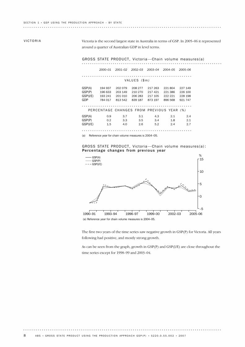
The first two years of the time series saw negative growth in GSP(P) for Victoria. All years
following had positive, and mostly strong growth.
As can be seen from the graph, growth in GSP(P) and GSP(I/E) are close throughout the
time series except for 1998–99 and 2003–04.
(a) Reference year for chain volume measures is 2004–05.
1990–91 1993–94 1996–97 1999–00 2002–03 2005–06
%
–5
0
5
10
15GSP(A)GSP(P)GSP(I/E)
GROSS STATE PRODUCT, Vic to r ia —Chain vo lume measures(a) :Percen tage changes from prev ious year
(a) Reference year for chain volume measures is 2004–05.
2.72.45.22.64.01.5GSP(I/E)2.11.83.43.53.30.2GSP(P)2.42.14.33.13.70.9GSP(A)
PE R C E N T A G E CH A N G E S FR O M PR E V I O U S YE A R (% )
921 747896 568873 197839 187813 542784 017GDP228 198222 221217 105206 283201 010193 241GSP(I/E)226 100221 386217 421210 270203 149196 633GSP(P)227 149221 804217 263208 277202 079194 937GSP(A)
VA L U E S ( $ m )
2005–062004–052003–042002–032001–022000–01
GROSS STATE PRODUCT, Vic to r ia —Chain vo lume measures(a)
Victoria is the second largest state in Australia in terms of GSP. In 2005–06 it represented
around a quarter of Australian GDP in level terms.
V I C T O R I A
8 A B S • GR O S S ST A T E P R O D U C T U S I N G T H E P R O D U C T I O N A P P R O A C H GS P ( P ) • 5 2 2 0 . 0 . 5 5 . 0 0 2 • 2 0 0 7
SE C T I O N 1 • G S P U S I N G T H E P R O D U C T I O N A P P R O A C H – B Y S T A T E

In 2005–06 the main industries that contributed to Victorian GSP growth were Property
and business services (0.6 percentage points), Construction, Finance and insurance,
Health and community services and Ownership of dwellings (each 0.3 percentage
points). The main negative contributing industry in 2005–06 was Manufacturing (–0.4
percentage points).
— nil or rounded to zero (including null cells)(a) Reference year for chain volume measures is 2004–05.
2.42.14.33.13.70.9GSP(A)0.20.30.9–0.50.30.6Statistical discrepancy0.20.30.30.60.4–0.2Taxes less subsidies on products0.30.30.30.30.30.3Ownership of dwellings0.20.1——0.10.1Personal & other services0.10.10.1—0.10.1Cultural & recreational services0.30.30.20.40.30.2Health & community services0.10.10.10.10.10.1Education————0.30.2
Government administration &defence
0.60.1–0.10.30.50.1Property & business services0.30.10.30.20.3—Finance & insurance0.20.10.20.30.1—Communication services0.10.30.10.40.10.3Transport & storage—0.10.2—0.1—
Accommodation, cafes &restaurants
—0.30.30.30.40.1Retail trade–0.10.10.60.7—–0.3Wholesale trade0.30.20.40.70.6–0.7Construction
–0.1——0.1—–0.1Electricity, gas & water supply–0.4–0.5–0.20.2–0.1–0.1Manufacturing–0.1–0.2—–0.2—–0.2Mining0.1–0.10.7–0.70.10.2Agriculture, forestry & fishing
% pts% pts% pts% pts% pts% pts
2005–062004–052003–042002–032001–022000–01
GSP, Vic to r ia —Chain vo lume measures (a) : Cont r i bu t i on to growth
Throughout the time series, the difference between GSP(A) and GSP(I/E) growth has
been less than 1.0 percentage point.
(a) Reference year for chain volume measures is 2004–05.
1990–91 1993–94 1996–97 1999–00 2002–03 2005–06
%
–4
–2
0
2
4
DIFFERENCE BETWEEN GSP(A) AND GSP( I /E ) , Percen tagechanges —Vic to r ia : Cha in vo lume measu res (a )
V I C T O R I A c o n t i n u e d
A B S • GR O S S ST A T E P R O D U C T U S I N G T H E P R O D U C T I O N A P P R O A C H GS P ( P ) • 5 2 2 0 . 0 . 5 5 . 0 0 2 • 2 0 0 7 9
SE C T I O N 1 • G S P U S I N G T H E P R O D U C T I O N A P P R O A C H – B Y S T A T E
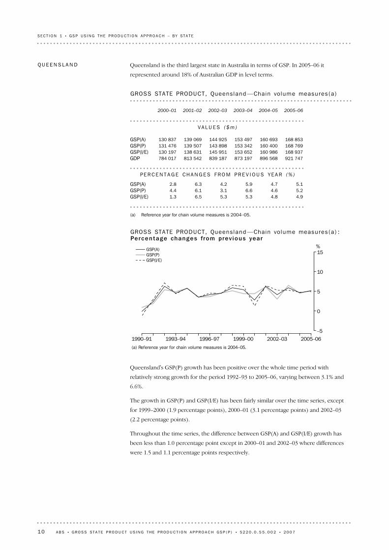
Queensland's GSP(P) growth has been positive over the whole time period with
relatively strong growth for the period 1992–93 to 2005–06, varying between 3.1% and
6.6%.
The growth in GSP(P) and GSP(I/E) has been fairly similar over the time series, except
for 1999–2000 (1.9 percentage points), 2000–01 (3.1 percentage points) and 2002–03
(2.2 percentage points).
Throughout the time series, the difference between GSP(A) and GSP(I/E) growth has
been less than 1.0 percentage point except in 2000–01 and 2002–03 where differences
were 1.5 and 1.1 percentage points respectively.
(a) Reference year for chain volume measures is 2004–05.
1990–91 1993–94 1996–97 1999–00 2002–03 2005–06
%
–5
0
5
10
15GSP(A)GSP(P)GSP(I/E)
GROSS STATE PRODUCT, Queens land —Chain vo lume measures (a) :Percen tage changes from prev ious year
(a) Reference year for chain volume measures is 2004–05.
4.94.85.35.36.51.3GSP(I/E)5.24.66.63.16.14.4GSP(P)5.14.75.94.26.32.8GSP(A)
PE R C E N T A G E CH A N G E S FR O M PR E V I O U S YE A R (% )
921 747896 568873 197839 187813 542784 017GDP168 937160 986153 652145 951138 631130 197GSP(I/E)168 769160 400153 342143 898139 507131 476GSP(P)168 853160 693153 497144 925139 069130 837GSP(A)
VA L U E S ( $ m )
2005–062004–052003–042002–032001–022000–01
GROSS STATE PRODUCT, Queens land —Chain vo lume measures (a)
Queensland is the third largest state in Australia in terms of GSP. In 2005–06 it
represented around 18% of Australian GDP in level terms.
QU E E N S L A N D
10 A B S • GR O S S ST A T E P R O D U C T U S I N G T H E P R O D U C T I O N A P P R O A C H GS P ( P ) • 5 2 2 0 . 0 . 5 5 . 0 0 2 • 2 0 0 7
SE C T I O N 1 • G S P U S I N G T H E P R O D U C T I O N A P P R O A C H – B Y S T A T E

In 2005–06, the main industries that contributed to Queensland GSP growth were
Property and business services (1.4 percentage points), Construction (0.7 percentage
points) and Finance and insurance (0.5 percentage points). Only Agriculture, forestry
and fishing and Mining (–0.1 percentage points) detracted from Queensland growth in
2005–06. Mining contribution to GSP(P) growth was flat in 2005–06 due to capacity
constraints limiting growth and an increase in lead, silver and zinc production being
offset by falls in copper and coal production.
— nil or rounded to zero (including null cells)(a) Reference year for chain volume measures is 2004–05.
5.14.75.94.26.32.8GSP(A)–0.20.1–0.61.10.2–1.5Statistical discrepancy0.10.20.30.40.4–0.2Taxes less subsidies on products0.30.40.30.30.30.3Ownership of dwellings0.10.1—–0.10.30.2Personal & other services—0.10.10.10.10.1Cultural & recreational services
0.30.30.30.20.30.3Health & community services0.2—0.20.10.10.2Education0.30.30.2–0.30.20.2
Government administration &defence
1.40.71.30.61.10.7Property & business services0.50.40.3—0.50.5Finance & insurance0.20.10.10.20.1—Communication services0.20.30.30.10.40.3Transport & storage0.3—0.30.2–0.20.2
Accommodation, cafes &restaurants
0.10.40.70.40.30.2Retail trade0.20.20.3—0.40.3Wholesale trade0.70.40.60.90.6–0.8Construction0.2—0.1—0.10.2Electricity, gas & water supply0.30.20.30.60.60.6Manufacturing
–0.10.60.3–0.10.51.2Mining–0.10.20.6–0.6–0.1—Agriculture, forestry & fishing
% pts% pts% pts% pts% pts% pts
2005–062004–052003–042002–032001–022000–01
GSP, Queens land —Chain vo lume measures (a) : Cont r i bu t i on togrowth
(a) Reference year for chain volume measures is 2004–05.
1990–91 1993–94 1996–97 1999–00 2002–03 2005–06
%
–4
–2
0
2
4
DIFFERENCE BETWEEN GSP(A) AND GSP( I /E ) , Percen tagechanges —Queens land : Cha in vo lume measu res (a )
QU E E N S L A N D c o n t i n u e d
A B S • GR O S S ST A T E P R O D U C T U S I N G T H E P R O D U C T I O N A P P R O A C H GS P ( P ) • 5 2 2 0 . 0 . 5 5 . 0 0 2 • 2 0 0 7 11
SE C T I O N 1 • G S P U S I N G T H E P R O D U C T I O N A P P R O A C H – B Y S T A T E
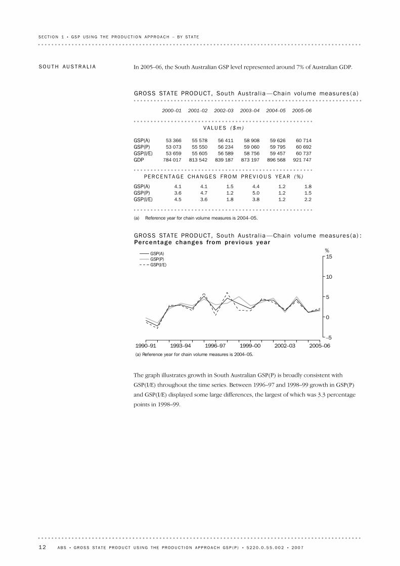
The graph illustrates growth in South Australian GSP(P) is broadly consistent with
GSP(I/E) throughout the time series. Between 1996–97 and 1998–99 growth in GSP(P)
and GSP(I/E) displayed some large differences, the largest of which was 3.3 percentage
points in 1998–99.
(a) Reference year for chain volume measures is 2004–05.
1990–91 1993–94 1996–97 1999–00 2002–03 2005–06
%
–5
0
5
10
15GSP(A)GSP(P)GSP(I/E)
GROSS STATE PRODUCT, South Aust ra l i a —Chain vo lume measures (a) :Percen tage changes from prev ious year
(a) Reference year for chain volume measures is 2004–05.
2.21.23.81.83.64.5GSP(I/E)1.51.25.01.24.73.6GSP(P)1.81.24.41.54.14.1GSP(A)
PE R C E N T A G E CH A N G E S FR O M PR E V I O U S YE A R (% )
921 747896 568873 197839 187813 542784 017GDP60 73759 45758 75656 58955 60553 659GSP(I/E)60 69259 79559 06056 23455 55053 073GSP(P)60 71459 62658 90856 41155 57853 366GSP(A)
VA L U E S ( $ m )
2005–062004–052003–042002–032001–022000–01
GROSS STATE PRODUCT, South Aust ra l i a —Chain vo lume measures (a)
In 2005–06, the South Australian GSP level represented around 7% of Australian GDP.SO U T H AU S T R A L I A
12 A B S • GR O S S ST A T E P R O D U C T U S I N G T H E P R O D U C T I O N A P P R O A C H GS P ( P ) • 5 2 2 0 . 0 . 5 5 . 0 0 2 • 2 0 0 7
SE C T I O N 1 • G S P U S I N G T H E P R O D U C T I O N A P P R O A C H – B Y S T A T E

In 2005–06, the main industries that contributed to South Australian GSP growth were
Agriculture, forestry and fishing (0.7 percentage points), Finance and insurance (0.5
percentage points), Health and community services and Ownership of dwellings (both
0.3 percentage points). The main negative contributing industries in 2005–06 were
Property and business services (–0.6 percentage points) and Mining (–0.3 percentage
points).
— nil or rounded to zero (including null cells)(a) Reference year for chain volume measures is 2004–05.
1.81.24.41.54.14.1GSP(A)0.2—–0.60.3–0.50.5Statistical discrepancy0.10.20.30.40.4–0.2Taxes less subsidies on products0.30.30.30.30.30.3Ownership of dwellings—–0.20.10.10.10.2Personal & other services—0.10.1——0.1Cultural & recreational services
0.30.30.20.30.30.4Health & community services0.20.1—0.10.2—Education—0.20.3–0.10.30.1
Government administration &defence
–0.6–0.40.50.30.90.4Property & business services0.5–0.1–0.3–0.50.30.8Finance & insurance0.20.10.10.10.1—Communication services
–0.10.10.40.40.10.1Transport & storage—–0.10.10.20.10.2
Accommodation, cafes &restaurants
—0.20.10.30.40.2Retail trade0.1—0.20.10.5–0.2Wholesale trade0.20.30.30.90.5–0.6Construction
–0.10.10.10.2——Electricity, gas & water supply——0.20.50.20.2Manufacturing
–0.30.30.1–0.1–0.30.3Mining0.7–0.41.5–1.70.41.4Agriculture, forestry & fishing
% pts% pts% pts% pts% pts% pts
2005–062004–052003–042002–032001–022000–01
GSP, South Aust ra l ia —Chain vo lume measures (a ) : Cont r i bu t i on togrowth
(a) Reference year for chain volume measures is 2004–05.
1990–91 1993–94 1996–97 1999–00 2002–03 2005–06
%
–4
–2
0
2
4
DIFFERENCE BETWEEN GSP(A) AND GSP( I /E ) , Percen tagechanges —South Aust ra l ia : Cha in vo lume measu res (a )
SO U T H AU S T R A L I A
c o n t i n u e d
A B S • GR O S S ST A T E P R O D U C T U S I N G T H E P R O D U C T I O N A P P R O A C H GS P ( P ) • 5 2 2 0 . 0 . 5 5 . 0 0 2 • 2 0 0 7 13
SE C T I O N 1 • G S P U S I N G T H E P R O D U C T I O N A P P R O A C H – B Y S T A T E

As illustrated by the graph, Western Australian GSP growth has been positive throughout
the time series with quite strong growth from 1992–93 onwards.
GSP(P) and GSP(I/E) growth rates generally display similar movements. However, in
some years there are large differences between the measures. For example, in 2003–04
the difference was 3.8 percentage points and in 2000–01 it was 3.1 percentage points.
(a) Reference year for chain volume measures is 2004–05.
1990–91 1993–94 1996–97 1999–00 2002–03 2005–06
%
–5
0
5
10
15GSP(A)GSP(P)GSP(I/E)
GROSS STATE PRODUCT, Weste rn Aust ra l ia —Chain vo lumemeasures (a) : Percen tage changes from prev ious year
(a) Reference year for chain volume measures is 2004–05.
4.94.77.65.45.5–0.8GSP(I/E)4.53.33.84.45.92.3GSP(P)4.74.05.74.95.70.8GSP(A)
PE R C E N T A G E CH A N G E S FR O M PR E V I O U S YE A R (% )
921 747896 568873 197839 187813 542784 017GDP107 910102 83798 26391 33386 63782 157GSP(I/E)106 571101 97798 69195 06391 07785 970GSP(P)107 241102 40798 47793 19888 85784 064GSP(A)
VA L U E S ( $ m )
2005–062004–052003–042002–032001–022000–01
GROSS STATE PRODUCT, Weste rn Aust ra l ia —Chain vo lumemeasures (a)
In 2005–06, the Western Australian GSP level represented around 12% of Australian GDP.WE S T E R N AU S T R A L I A
14 A B S • GR O S S ST A T E P R O D U C T U S I N G T H E P R O D U C T I O N A P P R O A C H GS P ( P ) • 5 2 2 0 . 0 . 5 5 . 0 0 2 • 2 0 0 7
SE C T I O N 1 • G S P U S I N G T H E P R O D U C T I O N A P P R O A C H – B Y S T A T E

Manufacturing, Construction (except in 2000–01 due to the introduction of the Goods
and Services Tax (GST)), Wholesale trade, Retail trade, and Transport and storage have
contributed positively to the growth in GSP since 2000–01. Some industries have had a
constant flat contribution, including Electricity, gas and water, Accommodation, cafes
and restaurants, Education and Cultural and recreational services.
In 2005–06, the main contributors to growth were Construction (1.5 percentage points),
Wholesale trade (0.7 percentage points) and Property and business services (0.5
percentage points). Mining detracted 0.4 percentage points from growth in 2005–06
mainly due to falls in production of crude oil and condensate, diamonds, gold and nickel.
— nil or rounded to zero (including null cells)(a) Reference year for chain volume measures is 2004–05.
4.74.05.74.95.70.8GSP(A)0.20.71.80.4–0.4–1.6Statistical discrepancy0.10.20.20.30.2–0.2Taxes less subsidies on products0.30.30.30.30.30.2Ownership of dwellings0.40.1———0.1Personal & other services—0.10.1———Cultural & recreational services
0.20.30.10.30.20.3Health & community services—0.10.1–0.10.10.1Education
–0.10.20.3—–0.20.1Government administration &
defence
0.50.2–0.40.81.70.5Property & business services0.2—–0.1–0.20.10.4Finance & insurance0.20.10.10.20.1—Communication services0.3—0.40.60.30.2Transport & storage———0.10.1—
Accommodation, cafes &restaurants
0.20.40.30.10.30.1Retail trade0.70.20.50.20.30.2Wholesale trade1.50.40.21.20.7–0.8Construction—0.1—0.1——Electricity, gas & water supply
0.20.30.60.90.80.6Manufacturing–0.41.1–2.31.00.41.6Mining0.3–0.31.9–1.10.5–0.8Agriculture, forestry & fishing
% pts% pts% pts% pts% pts% pts
2005–062004–052003–042002–032001–022000–01
GSP, Weste rn Aust ra l i a —Chain vo lume measures (a ) : Cont r i bu t i on togrowth
(a) Reference year for chain volume measures is 2004–05.
1990–91 1993–94 1996–97 1999–00 2002–03 2005–06
%
–4
–2
0
2
4
DIFFERENCE BETWEEN GSP(A) AND GSP( I /E ) , Percen tagechanges —Western Aust ra l i a : Cha in vo lume measu res (a )
WE S T E R N AU S T R A L I A
c o n t i n u e d
A B S • GR O S S ST A T E P R O D U C T U S I N G T H E P R O D U C T I O N A P P R O A C H GS P ( P ) • 5 2 2 0 . 0 . 5 5 . 0 0 2 • 2 0 0 7 15
SE C T I O N 1 • G S P U S I N G T H E P R O D U C T I O N A P P R O A C H – B Y S T A T E
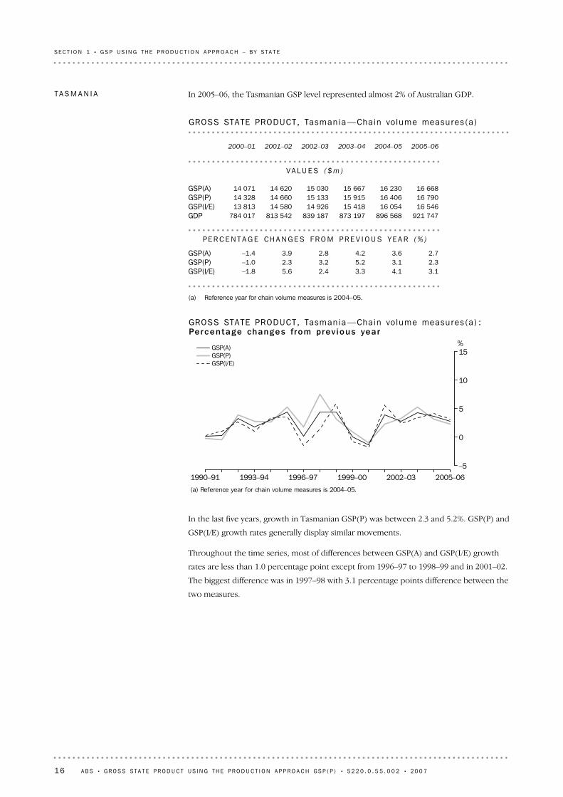
In the last five years, growth in Tasmanian GSP(P) was between 2.3 and 5.2%. GSP(P) and
GSP(I/E) growth rates generally display similar movements.
Throughout the time series, most of differences between GSP(A) and GSP(I/E) growth
rates are less than 1.0 percentage point except from 1996–97 to 1998–99 and in 2001–02.
The biggest difference was in 1997–98 with 3.1 percentage points difference between the
two measures.
(a) Reference year for chain volume measures is 2004–05.
1990–91 1993–94 1996–97 1999–00 2002–03 2005–06
%
–5
0
5
10
15GSP(A)GSP(P)GSP(I/E)
GROSS STATE PRODUCT, Tasman ia —Chain vo lume measures(a) :Percen tage changes from prev ious year
(a) Reference year for chain volume measures is 2004–05.
3.14.13.32.45.6–1.8GSP(I/E)2.33.15.23.22.3–1.0GSP(P)2.73.64.22.83.9–1.4GSP(A)
PE R C E N T A G E CH A N G E S FR O M PR E V I O U S YE A R (% )
921 747896 568873 197839 187813 542784 017GDP16 54616 05415 41814 92614 58013 813GSP(I/E)16 79016 40615 91515 13314 66014 328GSP(P)16 66816 23015 66715 03014 62014 071GSP(A)
VA L U E S ( $ m )
2005–062004–052003–042002–032001–022000–01
GROSS STATE PRODUCT, Tasman ia —Chain vo lume measures(a)
In 2005–06, the Tasmanian GSP level represented almost 2% of Australian GDP.TA S M A N I A
16 A B S • GR O S S ST A T E P R O D U C T U S I N G T H E P R O D U C T I O N A P P R O A C H GS P ( P ) • 5 2 2 0 . 0 . 5 5 . 0 0 2 • 2 0 0 7
SE C T I O N 1 • G S P U S I N G T H E P R O D U C T I O N A P P R O A C H – B Y S T A T E

In 2005–06, Manufacturing and Construction (0.6 percentage points) were the main
contributors to Tasmanian growth. Property and business services (–0.3 percentage
points), Mining (–0.2 percentage points) and Electricity, gas and water (–0.2 percentage
points) were the major detractors.
— nil or rounded to zero (including null cells)(a) Reference year for chain volume measures is 2004–05.
2.73.64.22.83.9–1.4GSP(A)0.30.5–1.0–0.41.6–0.4Statistical discrepancy0.10.20.30.40.4–0.2Taxes less subsidies on products0.30.30.30.30.30.2Ownership of dwellings—0.10.20.10.10.1Personal & other services—0.10.10.10.10.1Cultural & recreational services
0.30.20.2—0.80.2Health & community services0.10.10.20.10.10.1Education
–0.10.3–0.50.90.3–0.3Government administration &
defence
–0.30.51.0—–0.40.3Property & business services0.1–0.3–0.2–0.10.40.3Finance & insurance0.2—0.20.20.1—Communication services0.1—0.50.40.20.3Transport & storage—0.10.20.2–0.2–0.1
Accommodation, cafes &restaurants
0.40.40.60.20.20.2Retail trade0.30.20.20.3–0.3–0.4Wholesale trade0.60.20.7—0.9–0.4Construction
–0.20.3–0.20.1—–0.1Electricity, gas & water supply0.60.50.50.3–0.6–0.9Manufacturing
–0.2–0.10.1——–0.6Mining0.1—0.6–0.20.10.1Agriculture, forestry & fishing
% pts% pts% pts% pts% pts% pts
2005–062004–052003–042002–032001–022000–01
GSP, Tasman ia —Chain vo lume measures (a ) : Cont r i bu t i on to growth
(a) Reference year for chain volume measures is 2004–05.
1990–91 1993–94 1996–97 1999–00 2002–03 2005–06
%
–4
–2
0
2
4
DIFFERENCE BETWEEN GSP(A) AND GSP( I /E ) , Percen tagechanges —Tasman ia : Cha in vo lume measu res (a )
TA S M A N I A c o n t i n u e d
A B S • GR O S S ST A T E P R O D U C T U S I N G T H E P R O D U C T I O N A P P R O A C H GS P ( P ) • 5 2 2 0 . 0 . 5 5 . 0 0 2 • 2 0 0 7 17
SE C T I O N 1 • G S P U S I N G T H E P R O D U C T I O N A P P R O A C H – B Y S T A T E

Northern Territory GSP(P) growth has been quite variable throughout the time series as
illustrated by the graph.
GSP(P) and GSP(I/E) growth rates have shown similar growth rates over the period.
However, there have been some years with significant differences. In 1999–2000 GSP(P)
growth was 8.3% compared to 1.1% for GSP(I/E). In 2005–06 GSP(P) growth was 3.7%
and GSP(I/E) 7.5%.
(a) Reference year for chain volume measures is 2004–05.
1990–91 1993–94 1996–97 1999–00 2002–03 2005–06
%
–5
0
5
10
15GSP(A)GSP(P)GSP(I/E)
GROSS STATE PRODUCT, Nor thern Ter r i to r y —Chain vo lumemeasures (a) : Percen tage changes from prev ious year
(a) Reference year for chain volume measures is 2004–05.
7.56.00.20.21.65.5GSP(I/E)3.77.61.92.2–0.75.2GSP(P)5.56.81.01.20.45.4GSP(A)
PE R C E N T A G E CH A N G E S FR O M PR E V I O U S YE A R (% )
921 747896 568873 197839 187813 542784 017GDP11 47610 67810 07310 05110 0289 870GSP(I/E)11 45411 04810 26810 0809 8609 928GSP(P)11 46510 86310 17010 0669 9449 899GSP(A)
VA L U E S ( $ m )
2005–062004–052003–042002–032001–022000–01
GROSS STATE PRODUCT, Nor thern Ter r i to r y —Chain vo lumemeasures (a)
In 2005–06, the Northern Territory GSP level represented around 1% of Australian GDP.NO R T H E R N TE R R I T O R Y
18 A B S • GR O S S ST A T E P R O D U C T U S I N G T H E P R O D U C T I O N A P P R O A C H GS P ( P ) • 5 2 2 0 . 0 . 5 5 . 0 0 2 • 2 0 0 7
SE C T I O N 1 • G S P U S I N G T H E P R O D U C T I O N A P P R O A C H – B Y S T A T E

In 2005–06, Property and business services (2.7 percentage points) and Wholesale trade
(0.6 percentage points) were the largest positive contributors to the Northern Territory
GSP growth. Conversely, Manufacturing (–0.7 percentage points) and Government
administration (–0.4 percentage points) were the largest detractors from growth.
— nil or rounded to zero (including null cells)(a) Reference year for chain volume measures is 2004–05.
5.56.81.01.20.45.4GSP(A)1.7–0.9–0.8–1.01.10.1Statistical discrepancy0.10.20.20.20.2–0.2Taxes less subsidies on products0.30.40.30.30.30.3Ownership of dwellings0.40.10.1–0.3–0.20.1Personal & other services—0.20.20.30.10.1Cultural & recreational services
0.30.30.20.50.40.2Health & community services0.10.1—–0.10.1–0.1Education
–0.40.50.80.5–0.7–0.8Government administration &
defence
2.72.02.00.91.3–0.8Property & business services–0.1–0.2–0.2–0.20.20.3Finance & insurance0.10.10.10.20.1—Communication services0.20.50.3–0.1–0.10.1Transport & storage0.20.3–0.1–0.1–0.20.1
Accommodation, cafes &restaurants
—0.10.20.10.2—Retail trade0.6—–0.20.2–0.1–0.4Wholesale trade
–0.10.70.61.01.2–0.8Construction0.1—–0.1–0.10.1–0.1Electricity, gas & water supply
–0.7–0.30.30.80.70.6Manufacturing0.32.1–4.7–3.8–8.19.6Mining
–0.20.2–0.7–0.30.30.8Agriculture, forestry & fishing
% pts% pts% pts% pts% pts% pts
2005–062004–052003–042002–032001–022000–01
GSP, Nor thern Ter r i to r y —Chain vo lume measures (a ) : Cont r i bu t i on togrowth
In eleven out of the sixteen years in the time series, the differences between GSP(A) and
GSP(I/E) growth were less than 1.0 percentage point.
(a) Reference year for chain volume measures is 2004–05.
1990–91 1993–94 1996–97 1999–00 2002–03 2005–06
%
–4
–2
0
2
4
DIFFERENCE BETWEEN GSP(A) AND GSP( I /E ) , Percen tagechanges —Northern Ter r i to r y : Cha in vo lume measu res (a )
NO R T H E R N TE R R I T O R Y
c o n t i n u e d
A B S • GR O S S ST A T E P R O D U C T U S I N G T H E P R O D U C T I O N A P P R O A C H GS P ( P ) • 5 2 2 0 . 0 . 5 5 . 0 0 2 • 2 0 0 7 19
SE C T I O N 1 • G S P U S I N G T H E P R O D U C T I O N A P P R O A C H – B Y S T A T E

The Australian Capital Territory recorded strong growth over most of the period with
peaks in 1994–95 and 1998–99. GSP growth was negative on two occasions, 1991–92 and
1995–96.
Growth rates for GSP(P) and GSP(I/E) generally display similar movements. Some
differences from 1997–98 to 1999–2000 are evident.
(a) Reference year for chain volume measures is 2004–05.
1990–91 1993–94 1996–97 1999–00 2002–03 2005–06
%
–5
0
5
10
15GSP(A)GSP(P)GSP(I/E)
GROSS STATE PRODUCT, Aust ra l ian Capi ta l Ter r i to r y —Chain vo lumemeasures (a) : Percen tage changes from prev ious year
(a) Reference year for chain volume measures is 2004–05.
3.42.00.43.32.11.8GSP(I/E)4.43.51.83.11.92.8GSP(P)3.92.81.13.22.02.3GSP(A)
PE R C E N T A G E CH A N G E S FR O M PR E V I O U S YE A R (% )
921 747896 568873 197839 187813 542784 017GDP19 09818 47318 10818 02817 44317 083GSP(I/E)19 83519 00718 35618 03017 48917 170GSP(P)19 46718 74018 23218 02917 46617 127GSP(A)
VA L U E S ( $ m )
2005–062004–052003–042002–032001–022000–01
GROSS STATE PRODUCT, Aust ra l ian Capi ta l Ter r i to r y —Chain vo lumemeasures (a)
In 2005–06, the Australian Capital Territory GSP level represented around 2% of
Australian GDP.
AU S T R A L I A N CA P I T A L
TE R R I T O R Y
20 A B S • GR O S S ST A T E P R O D U C T U S I N G T H E P R O D U C T I O N A P P R O A C H GS P ( P ) • 5 2 2 0 . 0 . 5 5 . 0 0 2 • 2 0 0 7
SE C T I O N 1 • G S P U S I N G T H E P R O D U C T I O N A P P R O A C H – B Y S T A T E
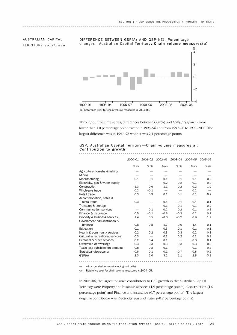
In 2005–06, the largest positive contributors to GSP growth in the Australian Capital
Territory were Property and business services (1.9 percentage points), Construction (1.0
percentage point) and Finance and insurance (0.7 percentage points). The largest
negative contributor was Electricity, gas and water (–0.2 percentage points).
— nil or rounded to zero (including null cells)(a) Reference year for chain volume measures is 2004–05.
3.92.81.13.22.02.3GSP(A)–0.6–0.8–0.70.10.1–0.5Statistical discrepancy–0.3–0.1—0.10.2–0.8Taxes less subsidies on products0.30.30.30.30.30.3Ownership of dwellings0.1–0.3—0.10.40.2Personal & other services0.20.20.20.2—0.3Cultural & recreational services0.30.20.30.30.20.2Health & community services
–0.10.10.10.3—0.1Education0.11.40.61.7–0.80.8
Government administration &defence
1.90.9–0.2–0.60.51.4Property & business services0.70.2–0.3–0.8–0.10.5Finance & insurance0.30.10.20.20.1—Communication services0.20.10.1–0.1——Transport & storage
–0.1–0.1–0.10.1—0.3Accommodation, cafes &
restaurants
0.20.10.10.10.30.3Retail trade—0.2——–0.10.2Wholesale trade
1.00.20.21.10.6–1.3Construction–0.2–0.10.2–0.2——Electricity, gas & water supply0.20.10.10.10.10.1Manufacturing——————Mining——————Agriculture, forestry & fishing
% pts% pts% pts% pts% pts% pts
2005–062004–052003–042002–032001–022000–01
GSP, Aust ra l ian Capi ta l Ter r i to r y —Chain vo lume measures (a ) :Cont r i bu t i on to growth
Throughout the time series, differences between GSP(A) and GSP(I/E) growth were
lower than 1.0 percentage point except in 1995–96 and from 1997–98 to 1999–2000. The
largest difference was in 1997–98 when it was 2.1 percentage points.
(a) Reference year for chain volume measures is 2004–05.
1990–91 1993–94 1996–97 1999–00 2002–03 2005–06
%
–4
–2
0
2
4
DIFFERENCE BETWEEN GSP(A) AND GSP( I /E ) , Percen tagechanges —Aust ra l ian Capi ta l Ter r i to r y : Cha in vo lume measu res (a )
AU S T R A L I A N CA P I T A L
TE R R I T O R Y c o n t i n u e d
A B S • GR O S S ST A T E P R O D U C T U S I N G T H E P R O D U C T I O N A P P R O A C H GS P ( P ) • 5 2 2 0 . 0 . 5 5 . 0 0 2 • 2 0 0 7 21
SE C T I O N 1 • G S P U S I N G T H E P R O D U C T I O N A P P R O A C H – B Y S T A T E

SECT I O N 2 GS P US I N G TH E PR O D U C T I O N AP P R O A C H –IN D U S T R Y GR O S S VA L U E AD D E D . . . . . . . . . . . . . . . . . . .
This section presents the scope, method and results used to produce GVA for each
ANZSIC93 industry division plus Ownership of dwellings and Taxes less subsidies on
products. ANZSIC93 breaks down each industry division into sub-divisions, groups and
classes. The estimates in this section are provided at division level. For some industries,
the compilation of GVA and its indicators are done at sub-division level, group or class
level and then aggregated to the division level. For further information about ANZSIC93,
please refer to ABS publication Australian and New Zealand Standard Industrial
Classification, 1993 (ANZSIC93) (cat. no. 1292.0.15.001).
For each industry the following information is provided:
! a definition and scope of the industry
! a description of the methods and data sources used to compile the estimates of GVA
! tables, graphs and analysis of volume GVA values and growth rates
! table and analysis of current price state shares of GVA.
The primary focus is on presenting the results, however, some analysis is also provided
for each industry.
I N T R O D U C T I O N
22 A B S • GR O S S ST A T E P R O D U C T U S I N G T H E P R O D U C T I O N A P P R O A C H GS P ( P ) • 5 2 2 0 . 0 . 5 5 . 0 0 2 • 2 0 0 7

The methodology for Agriculture, forestry and fishing uses a combination of double
deflation and quantity revaluation.
The sub-divisions Agriculture and Services to agriculture are compiled together using the
double deflation approach. That is, the volume measures of intermediate input are
subtracted from volume measures of output, both valued in the prices of the previous
year, to derive volume measures of GVA.
The sub-divisions Forestry and logging and Commercial fishing are compiled separately
using the quantity revaluation approach.
The main source of data on state Agriculture outputs and most inputs is the ABS
collection, Value of Agricultural Commodities Produced, Australia (VACP)
(cat. no. 7503.0). For Forestry and fishing and some of the Agriculture inputs, Australian
Bureau of Agricultural and Resource Economics (ABARE) data are used.
The double deflation method is used for all but the latest year for Agriculture and
Services to agriculture as the VACP collection is released with a lag of one year. For the
latest year, the method for all of Agriculture, forestry and fishing sub-divisions is an
output indicator approach. ABARE forecasts of production, of the major agricultural
commodities in each state, are used as the output indicator. The volume movements in
the major commodities in each individual state are obtained using quantity revaluation.
These are used to extrapolate reference year volume estimates of GVA by state for
Agriculture, forestry and fishing. The state volume GVAs are benchmarked to the annual
national industry volume GVA.
Summary of GSP(P)
sources and methods
The Agriculture, forestry and fishing industry engages in activities such as breeding,
keeping and cultivation of plants and animals; afforestation, harvesting and gathering of
forestry products; and catching, gathering and breeding of marine life.
ANZSIC93 Division A, Agriculture, forestry and fishing, consists of four sub-divisions:
! Agriculture (sub-division 01)
! Services to agriculture (sub-division 02)
! Forestry and logging (sub-division 03)
! Commercial fishing (sub-division 04).
AG R I C U L T U R E , FO R E S T R Y
AN D F I S H I N G
Definit ion and scope
A B S • GR O S S ST A T E P R O D U C T U S I N G T H E P R O D U C T I O N A P P R O A C H GS P ( P ) • 5 2 2 0 . 0 . 5 5 . 0 0 2 • 2 0 0 7 23
SE C T I O N 2 • G S P U S I N G T H E P R O D U C T I O N A P P R O A C H – I N D U S T R Y G R O S S V A L U E A D D E D

(a) At basic prices(b) Reference year for chain volume measures is 2004–05.
1990–91 1993–94 1996–97 1999–00 2002–03 2005–06
%
–60
–40
–20
0
20
40
60
80AustraliaNew South WalesVictoria
AGRICULTURE, FORESTRY AND FISHING GROSS VALUE ADDED (a) ,Cha in vo lume measures (b )–Percentage changes
(a) At basic prices.(b) Reference year for chain volume measures is 2004–05.
3.7–0.731.4–23.53.24.0Australia1.40.326.1–0.7–10.120.6Australian Capital Territory
–7.74.7–18.0–8.16.623.4Northern Territory2.1–0.18.3–2.71.41.2Tasmania7.7–8.274.9–29.114.4–18.6Western Australia
12.9–6.430.7–25.86.726.7South Australia–2.63.918.1–13.9–2.6–0.4Queensland3.7–3.027.1–21.41.65.9Victoria3.16.929.0–32.31.17.5New South Wales
PE R C E N T A G E CH A N G E S FR O M PR E V I O U S YE A R (% )
28 15127 15327 34020 80727 19426 363Australia191919151517Australian Capital Territory
302327312381414388Northern Territory1 0881 0651 0669841 011997Tasmania4 0683 7774 1162 3543 3212 902Western Australia3 7733 3433 5722 7333 6843 454South Australia5 7785 9305 7054 8305 6085 755Queensland6 7856 5446 7495 3096 7516 647Victoria6 3396 1475 7514 4576 5866 512New South Wales
VA L U E S ( $ m )
2005–062004–052003–042002–032001–022000–01
AGRICULTURE, FORESTRY AND FISHING GROSS VALUE ADDED (a) ,Cha in vo lume measures (b )
Results for Agr iculture,
forestry and fishing
24 A B S • GR O S S ST A T E P R O D U C T U S I N G T H E P R O D U C T I O N A P P R O A C H GS P ( P ) • 5 2 2 0 . 0 . 5 5 . 0 0 2 • 2 0 0 7
SE C T I O N 2 • G S P U S I N G T H E P R O D U C T I O N A P P R O A C H – I N D U S T R Y G R O S S V A L U E A D D E D

Throughout the time series, all states except Tasmania, the Northern Territory and the
Australian Capital Territory exhibited a similar growth pattern to the Australia series.
Overall, the growth in the agricultural industry is variable due to the impact of weather
patterns on the industry. The two droughts in 1994–95 and 2002–03 had strong negative
(a) At basic prices.(b) Reference year for chain volume measures is 2004–05.
1990–91 1993–94 1996–97 1999–00 2002–03 2005–06
%
–60
–40
–20
0
20
40
60
80AustraliaNorthern TerritoryAustralian Capital Territory
AGRICULTURE, FORESTRY AND FISHING GROSS VALUE ADDED (a) ,Cha in vo lume measures (b )–Percentage changes
(a) At basic prices.(b) Reference year for chain volume mesaures is 2004–05.
1990–91 1993–94 1996–97 1999–00 2002–03 2005–06
%
–60
–40
–20
0
20
40
60
80AustraliaWestern AustraliaTasmania
AGRICULTURE, FORESTRY AND FISHING GROSS VALUE ADDED (a) ,Cha in vo lume measures (b )–Percentage changes
(a) At basic prices.(b) Reference year for chain volume measures is 2004–05.
1990–91 1993–94 1996–97 1999–00 2002–03 2005–06
%
–60
–40
–20
0
20
40
60
80AustraliaQueenslandSouth Australia
AGRICULTURE, FORESTRY AND FISHING GROSS VALUE ADDED (a) ,Cha in vo lume measures (b )–Percentage changes
Results for Agr iculture,
forestry and fishing
cont inue d
A B S • GR O S S ST A T E P R O D U C T U S I N G T H E P R O D U C T I O N A P P R O A C H GS P ( P ) • 5 2 2 0 . 0 . 5 5 . 0 0 2 • 2 0 0 7 25
SE C T I O N 2 • G S P U S I N G T H E P R O D U C T I O N A P P R O A C H – I N D U S T R Y G R O S S V A L U E A D D E D

Victoria, Queensland and New South Wales accounted for around 68% of Australian
Agriculture, forestry and fishing GVA in 2005–06. New South Wales share of the industry
has gradually decreased throughout the time series from 29.6% in 1989–90 to 20.6% in
2005–06. All other states increased their share over this period except for the Australian
Capital Territory which recorded stable industry shares throughout the time series.
100.0100.0100.0100.0100.0100.0Australia0.10.10.10.10.10.1
Australian CapitalTerritory
1.11.21.11.51.10.5Northern Territory4.13.93.53.74.73.8Tasmania
14.013.916.514.415.413.4Western Australia12.812.314.512.111.011.1South Australia22.121.818.721.422.220.1Queensland24.124.123.421.821.521.5Victoria21.722.622.224.924.129.6New South Wales
%%%%%%
2005–062004–052003–041999–001994–951989–90
AGRICULTURE, FORESTRY AND FISHING GROSS VALUE ADDED, Stateshares —Cur ren t pr ices
impacts on growth. During the 1994–95 drought all states except the Northern Territory
experienced negative growth. The 2002–03 drought saw all states having negative growth
with New South Wales, Western Australia, South Australia and Victoria showing the
largest negative growth. Most states showed large positive growth in the years following
the droughts.
Results for Agr iculture,
forestry and fishing
cont inue d
26 A B S • GR O S S ST A T E P R O D U C T U S I N G T H E P R O D U C T I O N A P P R O A C H GS P ( P ) • 5 2 2 0 . 0 . 5 5 . 0 0 2 • 2 0 0 7
SE C T I O N 2 • G S P U S I N G T H E P R O D U C T I O N A P P R O A C H – I N D U S T R Y G R O S S V A L U E A D D E D

Sub-divisions 11, 12 and 13 are compiled together, while sub-division 15, Services to
mining is compiled separately. Sub-division 14, Other mining, is not compiled for each
state due to a lack of consistent state level data. Instead the national total for Sub-division
14 is allocated across states based on Mining GVA movements for all other sub-divisions.
The methodology for Mining uses an output indicator approach to compile state by
industry GVA estimates. Mining output volumes are derived by the quantity revaluation
method except for Services to mining, which is derived by price deflation. State level
value added is compiled for individual mineral groups before being aggregated to
division level.
Sub-divisions 11, 12 and 13 use quantity revaluation compiled at the mineral group level
(e.g. coal, gold, iron etc.). State production values of each mineral, sourced from the ABS
collection Mining Operations, Australia (cat. no. 8415.0), are quantity revalued using
production quantities from the same collection. The volume estimates are then used to
allocate national value added by mineral across the states. In the most recent year,
Mining Operations data are not available. Data from ABARE are used to provide the
latest year estimate for each mineral group.
Estimates of sub-division 15, Services to mining, are derived by splitting the national
Services to mining value added estimates using state quarterly Business Indicators,
Australia (QBIS) (cat. no. 5676.0) turnover data for Services to mining. The estimates
are then price deflated using the same deflator used in the quarterly national estimates.
This deflator is a combination of seven price indexes. Six components are from ABS
Producer Price Indexes, Australia (PPI) (cat. no. 6427.0), and the seventh component,
which receives the highest weight, is the wage cost index for the hourly wage rate in the
mining industry, obtained from the ABS collection Labour Price Index, Australia
(cat. no. 6345.0).
The value added estimates for each state, by each mineral plus Services to mining, are
summed to Mining division level and used to derive volume measures of GVA for Mining.
The state volume GVAs are benchmarked to the annual national industry volume GVA.
Summary of GSP(P)
sources and methods
The Mining industry comprises units mainly engaged in mining, in exploration for
minerals, and in the provision of a wide variety of services to mining and mineral
exploration.
ANZSIC93 Division B, Mining, consists of five sub-divisions:
! Coal mining (sub-division 11)
! Oil and gas extraction (sub-division 12)
! Metal ore mining (sub-division 13)
! Other mining (sub-division 14)
! Services to mining (sub-division 15).
MI N I N G
Definit ion and scope
A B S • GR O S S ST A T E P R O D U C T U S I N G T H E P R O D U C T I O N A P P R O A C H GS P ( P ) • 5 2 2 0 . 0 . 5 5 . 0 0 2 • 2 0 0 7 27
SE C T I O N 2 • G S P U S I N G T H E P R O D U C T I O N A P P R O A C H – I N D U S T R Y G R O S S V A L U E A D D E D
(a) At basic prices.(b) Reference year for chain volume measures is 2004–05.
1990–91 1993–94 1996–97 1999–00 2002–03 2005–06
%
–20
–10
0
10
20
30AustraliaNew South WalesVictoria
MINING GROSS VALUE ADDED (a) , Cha in vo lumemeasures (b )–Percentage changes
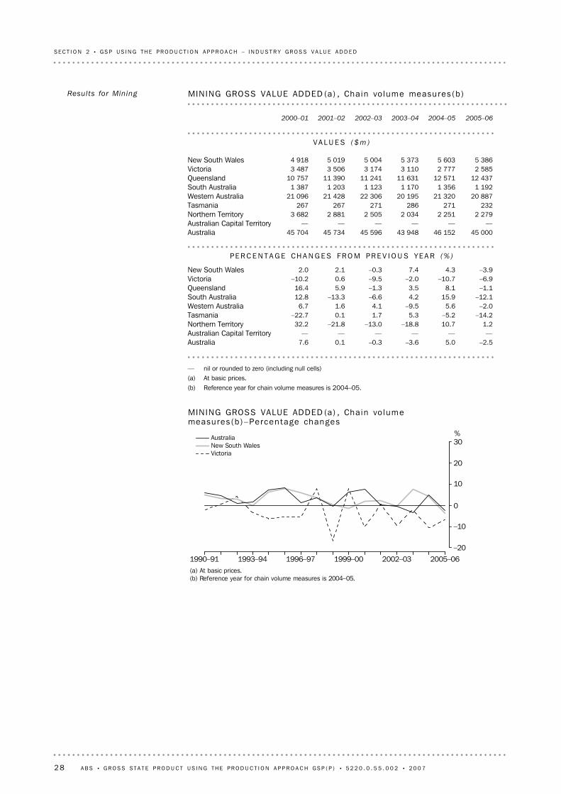
— nil or rounded to zero (including null cells)(a) At basic prices.(b) Reference year for chain volume measures is 2004–05.
–2.55.0–3.6–0.30.17.6Australia——————Australian Capital Territory
1.210.7–18.8–13.0–21.832.2Northern Territory–14.2–5.25.31.70.1–22.7Tasmania
–2.05.6–9.54.11.66.7Western Australia–12.115.94.2–6.6–13.312.8South Australia
–1.18.13.5–1.35.916.4Queensland–6.9–10.7–2.0–9.50.6–10.2Victoria–3.94.37.4–0.32.12.0New South Wales
PE R C E N T A G E CH A N G E S FR O M PR E V I O U S YE A R (% )
45 00046 15243 94845 59645 73445 704Australia——————Australian Capital Territory
2 2792 2512 0342 5052 8813 682Northern Territory232271286271267267Tasmania
20 88721 32020 19522 30621 42821 096Western Australia1 1921 3561 1701 1231 2031 387South Australia
12 43712 57111 63111 24111 39010 757Queensland2 5852 7773 1103 1743 5063 487Victoria5 3865 6035 3735 0045 0194 918New South Wales
VA L U E S ( $ m )
2005–062004–052003–042002–032001–022000–01
MINING GROSS VALUE ADDED (a) , Cha in vo lume measures (b )Results for Mining
28 A B S • GR O S S ST A T E P R O D U C T U S I N G T H E P R O D U C T I O N A P P R O A C H GS P ( P ) • 5 2 2 0 . 0 . 5 5 . 0 0 2 • 2 0 0 7
SE C T I O N 2 • G S P U S I N G T H E P R O D U C T I O N A P P R O A C H – I N D U S T R Y G R O S S V A L U E A D D E D

(a) At basic prices.(b) Reference year for chain volume measures is 2004–05.
1990–91 1993–94 1996–97 1999–00 2002–03 2005–06
%
–30
–15
0
15
30
45
60AustraliaNorthern Territory
MINING GROSS VALUE ADDED (a) , Cha in vo lumemeasures (b )–Percentage changes
(a) At basic prices.(b) Reference year for chain volume measures is 2004–05.
1990–91 1993–94 1996–97 1999–00 2002–03 2005–06
%
–20
–10
0
10
20
30AustraliaWestern AustraliaTasmania
MINING GROSS VALUE ADDED (a) , Cha in vo lumemeasures (b )–Percentage changes
(a) At basic prices.(b) Reference year for chain volume measures is 2004–05.
1990–91 1993–94 1996–97 1999–00 2002–03 2005–06
%
–20
–10
0
10
20
30AustraliaQueenslandSouth Australia
MINING GROSS VALUE ADDED (a) , Cha in vo lumemeasures (b )–Percentage changes
Results for Mining
cont inue d
A B S • GR O S S ST A T E P R O D U C T U S I N G T H E P R O D U C T I O N A P P R O A C H GS P ( P ) • 5 2 2 0 . 0 . 5 5 . 0 0 2 • 2 0 0 7 29
SE C T I O N 2 • G S P U S I N G T H E P R O D U C T I O N A P P R O A C H – I N D U S T R Y G R O S S V A L U E A D D E D

Western Australia and Queensland together accounted for around 76% of Australian
Mining GVA in 2005–06. Western Australia has significantly increased its share from
29.6% in 1989–90 to 45.2% in 2005–06 while Queensland increased its share from 21.8%
in 1989–90 to 30.8% in 2005–06. Victoria has gradually lost industry share throughout the
period, falling from 19.2% in 1989–90 to 5.3% in 2005–06 as a result of falling oil
production from the Bass Strait oil fields.
— nil or rounded to zero (including null cells)
100.0100.0100.0100.0100.0100.0Australia——————
Australian CapitalTerritory
4.64.95.15.53.75.8Northern Territory0.50.60.60.81.31.6Tasmania
45.246.244.844.641.629.6Western Australia2.72.92.94.04.14.6South Australia
30.827.224.520.718.321.8Queensland5.36.09.311.216.319.2Victoria
10.912.112.713.114.717.4New South Wales
%%%%%%
2005–062004–052003–041999–001994–951989–90
MINING GROSS VALUE ADDED, State shares —Curren t pr ices
Western Australia has shown the strongest growth throughout the time series.
Queensland has also shown strong growth over the time series with positive growth in
seven of the last eight years. Victoria and Tasmania are characterised by an overall
decrease in growth while South Australia has displayed variable growth. New South
Wales has had fairly flat growth throughout the time series.
The Northern Territory had extremely high growth in 1999–2000 and 2000–01 following
the completion of a major mining project, but experienced strong decreases in the
following three years due to falling offshore oil production. In 2005–06, Mining
decreased in all states except the Northern Territory (up 1.2%) reflecting the overall
decrease in Australian GVA for Mining of 2.5%.
Results for Mining
cont inue d
30 A B S • GR O S S ST A T E P R O D U C T U S I N G T H E P R O D U C T I O N A P P R O A C H GS P ( P ) • 5 2 2 0 . 0 . 5 5 . 0 0 2 • 2 0 0 7
SE C T I O N 2 • G S P U S I N G T H E P R O D U C T I O N A P P R O A C H – I N D U S T R Y G R O S S V A L U E A D D E D

The methodology for Manufacturing uses an output indicator approach to compile state
by industry GVA estimates. Manufacturing output volumes are derived by deflating sales
estimates for the various manufacturing activities at a sub-division level. The output
indicators form the basis upon which volume measures of value added are derived at the
division level.
The current price state estimates of Manufacturing output are obtained from the annual
ABS Manufacturing Industry, Australia (cat. no. 8221.0) for all but the latest two years.
Since the survey is released approximately two years after the reference period, QBIS
data are used to extrapolate the current price Manufacturing output data for the latest
two years. Therefore, estimates for the most recent two years have the potential to be
subject to considerable revision when the Manufacturing Survey data become available.
The current price output estimates are price deflated using Manufacturing sub-division
price indexes, obtained from ABS PPI. National level price indexes are used as no state
level indexes are available.
This method is used for each Manufacturing sub-division except for 'Petroleum, coal,
chemical and associated product manufacturing' which is quantity revalued using
quantities of automotive gasoline, aviation turbine and automotive diesel obtained from
the Department of Industry, Tourism and Resources (DITR) publication Australian
Petroleum Statistics. The volume estimates of output by Manufacturing sub-division for
each state are then summed to the Manufacturing division level.
The state output indicators are used to derive volume measures of GVA for
Manufacturing. The state volume GVAs are benchmarked to the annual national industry
volume GVA.
Summary of GSP(P)
sources and methods
In a broad sense manufacturing activity relates to the physical or chemical transformation
of materials or components into new products, whether the work is performed by power
driven machines or by hand.
ANZSIC Division C, Manufacturing, consists of nine sub-divisions:
! Food, beverage and tobacco manufacturing (sub-division 21)
! Textile, clothing, footwear and leather manufacturing (sub-division 22)
! Wood and paper product manufacturing (sub-division 23)
! Printing, publishing and recorded media (sub-division 24)
! Petroleum, coal, chemical and associated product manufacturing (sub-division 25)
! Non-metallic mineral product manufacturing (sub-division 26)
! Metal product manufacturing (sub-division 27)
! Machinery and equipment manufacturing (sub-division 28)
! Other manufacturing (sub-division 29).
MA N U F A C T U R I N G
Definit ion and scope
A B S • GR O S S ST A T E P R O D U C T U S I N G T H E P R O D U C T I O N A P P R O A C H GS P ( P ) • 5 2 2 0 . 0 . 5 5 . 0 0 2 • 2 0 0 7 31
SE C T I O N 2 • G S P U S I N G T H E P R O D U C T I O N A P P R O A C H – I N D U S T R Y G R O S S V A L U E A D D E D

(a) At basic prices.(b) Reference year for chain volume measures is 2004–05.
1990–91 1993–94 1996–97 1999–00 2002–03 2005–06
%
–20
–10
0
10
20
30AustraliaNew South WalesVictoria
MANUFACTURING GROSS VALUE ADDED (a) , Cha in vo lumemeasures (b )–Percentage changes
— nil or rounded to zero (including null cells)(a) At basic prices.(b) Reference year for chain volume measures is 2004–05.
–0.4–1.10.93.62.12.2Australia7.76.46.68.26.88.6Australian Capital Territory
–10.6–4.53.812.212.610.1Northern Territory4.43.43.42.3–3.8–5.7Tasmania2.83.47.412.110.48.2Western Australia0.1—1.53.51.11.4South Australia3.41.63.16.45.96.6Queensland
–3.1–3.3–1.21.1–0.9–0.5Victoria–0.7–2.0–0.22.61.42.0New South Wales
PE R C E N T A G E CH A N G E S FR O M PR E V I O U S YE A R (% )
96 01296 36697 42296 52893 13391 195Australia402373350329304284Australian Capital Territory630705739712634563Northern Territory
2 3992 2982 2232 1512 1022 184Tasmania8 6108 3808 1027 5446 7316 095Western Australia8 4228 4098 4138 2858 0067 917South Australia
15 10614 61214 38113 94813 10912 381Queensland28 45329 36530 37730 75130 42330 699Victoria31 98932 22432 87532 93132 10631 674New South Wales
VA L U E S ( $ m )
2005–062004–052003–042002–032001–022000–01
MANUFACTURING GROSS VALUE ADDED (a) , Cha in vo lume measures (b )Results for Manufacturing
32 A B S • GR O S S ST A T E P R O D U C T U S I N G T H E P R O D U C T I O N A P P R O A C H GS P ( P ) • 5 2 2 0 . 0 . 5 5 . 0 0 2 • 2 0 0 7
SE C T I O N 2 • G S P U S I N G T H E P R O D U C T I O N A P P R O A C H – I N D U S T R Y G R O S S V A L U E A D D E D

(a) At basic prices.(b) Reference year for chain volume measures is 2004–05.
1990–91 1993–94 1996–97 1999–00 2002–03 2005–06
%
–20
–10
0
10
20
30AustraliaNorthern TerritoryAustralian Capital Territory
MANUFACTURING GROSS VALUE ADDED (a) , Cha in vo lumemeasures (b )–Percentage changes
(a) At basic prices.(b) Reference year for chain volume measures is 2004–05.
1990–91 1993–94 1996–97 1999–00 2002–03 2005–06
%
–20
–10
0
10
20
30AustraliaWestern AustraliaTasmania
MANUFACTURING GROSS VALUE ADDED (a) , Cha in vo lumemeasures (b )–Percentage changes
(a) At basic prices.(b) Reference year for chain volume measures is 2004–05.
1990–91 1993–94 1996–97 1999–00 2002–03 2005–06
%
–20
–10
0
10
20
30AustraliaQueenslandSouth Australia
MANUFACTURING GROSS VALUE ADDED (a) , Cha in vo lumemeasures (b )–Percentage changes
Results for Manufacturing
cont inue d
A B S • GR O S S ST A T E P R O D U C T U S I N G T H E P R O D U C T I O N A P P R O A C H GS P ( P ) • 5 2 2 0 . 0 . 5 5 . 0 0 2 • 2 0 0 7 33
SE C T I O N 2 • G S P U S I N G T H E P R O D U C T I O N A P P R O A C H – I N D U S T R Y G R O S S V A L U E A D D E D

The Australian Manufacturing industry is dominated by New South Wales and Victoria
which together accounted for 63.1% of Australian Manufacturing GVA in 2005–06. New
South Wales has slightly increased its share from 32.1% in 1989–90 to 33.1% in 2005–06
but the share has been stable at around 33% for most of the time series. Victoria and
South Australia have decreased their shares throughout the time series. Victoria's share
went from 33.4% to 30.0% and South Australia went from 10.0% to 8.9%. Queensland has
gradually increased its share throughout the time series from 12.3% in 1989–90 to 15.5%
in 2005–06. The other states shares have remained stable.
100.0100.0100.0100.0100.0100.0Australia0.40.40.40.30.40.4
Australian CapitalTerritory
0.70.70.80.70.70.6Northern Territory2.42.42.42.32.32.6Tasmania9.08.78.68.98.08.6Western Australia8.98.78.98.59.110.0South Australia
15.515.214.813.813.712.3Queensland30.030.530.531.332.033.4Victoria33.133.433.634.333.832.1New South Wales
%%%%%%
2005–062004–052003–041999–001994–951989–90
MANUFACTURING GROSS VALUE ADDED, State shares —Current pr ices
Throughout the time series, New South Wales, Victoria, Queensland and South Australia
have exhibited a similar growth pattern to the overall Australia series, while Western
Australia, Tasmania and the Northern Territory followed the Australian pattern until
1998–99 and then diverged. Queensland recorded positive Manufacturing growth
throughout the time series with a peak recorded in 1993–94.
Results for Manufacturing
cont inue d
34 A B S • GR O S S ST A T E P R O D U C T U S I N G T H E P R O D U C T I O N A P P R O A C H GS P ( P ) • 5 2 2 0 . 0 . 5 5 . 0 0 2 • 2 0 0 7
SE C T I O N 2 • G S P U S I N G T H E P R O D U C T I O N A P P R O A C H – I N D U S T R Y G R O S S V A L U E A D D E D

The methodology for Electricity, gas and water uses an output indicator approach to
compile state by industry GVA estimates. Output volumes are derived using quantity
revaluation of the state output indicators. The output volumes then form the basis upon
which volume measures of GVA are derived at the division level.
Quantity data by state for the Electricity class are sourced from the quarterly ABS
Manufacturing Industry.
Price data for the Electricity class are obtained from a number of sources including the
National Electricity Market Management Company (NEMMCO) and the Electricity Supply
Association of Australia (prior to 1999–2000). The NEMMCO price data are not available
for Western Australia and the Northern Territory. The average price for all other states
has been used for these two states.
The quantity of gas produced by state is sourced from the quarterly ABS Manufacturing
Industry. State gas price data were previously sourced from the Australian Gas
Association. As these data are not available after 1997–98, Consumer Price Index,
Australia (CPI) (cat. no. 6401.0) gas data have been used to extrapolate data from
1997–98.
Water and sewerage current price data and volumes are sourced from various water
authorities in New South Wales, Victoria, Queensland and South Australia.
For the remaining states, the average consumption per head of population of New South
Wales, Victoria, Queensland and South Australia was used with population estimates to
obtain current price and volume data.
The component level output estimates are summed and then chained to form a total
Electricity, gas and water volume output indicator by state. The state output indicators
are used to derive volume measures of GVA for Electricity, gas and water. The state
volume GVAs are then benchmarked to the annual national industry volume GVA.
Summary of GSP(P)
sources and methods
The Electricity, gas and water supply industry includes all units mainly engaged in the
generation, transmission or distribution of electricity; manufacture of town gas from coal
and/or petroleum or the distribution of the manufactured town gas, natural gas or
liquefied petroleum gas through a mains reticulation system; the storage, purification or
supply of water; or the operation of sewerage or drainage systems including sewerage
treatment plants.
ANZSIC93 Division D, Electricity, gas and water supply, consists of two sub-divisions:
! Electricity and gas supply (sub-division 36)
! Water supply, sewerage and drainage services (sub-division 37).
EL E C T R I C I T Y , GA S AN D
WA T E R SU P P L Y
Definit ion and scope
A B S • GR O S S ST A T E P R O D U C T U S I N G T H E P R O D U C T I O N A P P R O A C H GS P ( P ) • 5 2 2 0 . 0 . 5 5 . 0 0 2 • 2 0 0 7 35
SE C T I O N 2 • G S P U S I N G T H E P R O D U C T I O N A P P R O A C H – I N D U S T R Y G R O S S V A L U E A D D E D

(a) At basic prices.(b) Reference year for chain volume measures is 2004–05.
1990–91 1993–94 1996–97 1999–00 2002–03 2005–06
%
–20
–10
0
10
20
30AustraliaNew South WalesVictoria
ELECTR IC ITY , GAS AND WATER GROSS VALUE ADDED (a) , Cha invo lume measures (b )–Percentage changes
(a) At basic prices.(b) Reference year for chain volume measures is 2004–05.
2.00.70.70.9–0.81.5Australia–6.4–3.87.5–6.91.11.5Australian Capital Territory3.52.0–3.0–2.53.7–2.7Northern Territory
–4.17.4–3.41.5–0.4–0.9Tasmania–0.13.81.54.51.51.1Western Australia–4.52.94.55.8–1.40.4South Australia9.4–2.34.6–1.84.07.1Queensland
–1.81.7–1.51.8–0.4–2.8Victoria6.4–1.3–0.5–1.2–4.74.6New South Wales
PE R C E N T A G E CH A N G E S FR O M PR E V I O U S YE A R (% )
20 54920 14720 00019 86719 69019 840Australia422451469436468463Australian Capital Territory186180176182186180Northern Territory733765712738727730Tasmania
2 7282 7322 6302 5912 4802 443Western Australia1 5801 6561 6091 5401 4551 476South Australia3 2022 9282 9952 8642 9162 803Queensland5 6195 7235 6265 7145 6145 635Victoria6 0795 7145 7915 8225 8906 181New South Wales
VA L U E S ( $ m )
2005–062004–052003–042002–032001–022000–01
ELECTRIC ITY , GAS AND WATER GROSS VALUE ADDED (a) , Cha in vo lumemeasures (b )
Results for Electr ic i ty, gas
and water
36 A B S • GR O S S ST A T E P R O D U C T U S I N G T H E P R O D U C T I O N A P P R O A C H GS P ( P ) • 5 2 2 0 . 0 . 5 5 . 0 0 2 • 2 0 0 7
SE C T I O N 2 • G S P U S I N G T H E P R O D U C T I O N A P P R O A C H – I N D U S T R Y G R O S S V A L U E A D D E D

(a) At basic prices.(b) Reference year for chain volume measures is 2004–05.
1990–91 1993–94 1996–97 1999–00 2002–03 2005–06
%
–20
–10
0
10
20
30AustraliaNorthern TerritoryAustralian Capital Territory
ELECTR IC ITY , GAS AND WATER GROSS VALUE ADDED (a) , Cha invo lume measures (b )–Percentage changes
(a) At basic prices.(b) Reference year for chain volume measures is 2004–05.
1990–91 1993–94 1996–97 1999–00 2002–03 2005–06
%
–20
–10
0
10
20
30AustraliaWestern AustraliaTasmania
ELECTR IC ITY , GAS AND WATER GROSS VALUE ADDED (a) , Cha invo lume measures (b )–Percentage changes
(a) At basic prices.(b) Reference year for chain volume measures is 2004–05.
1990–91 1993–94 1996–97 1999–00 2002–03 2005–06
%
–20
–10
0
10
20
30AustraliaQueenslandSouth Australia
ELECTR IC ITY , GAS AND WATER GROSS VALUE ADDED (a) , Cha invo lume measures (b )–Percentage changes
Results for Electr ic i ty, gas
and water cont inued
A B S • GR O S S ST A T E P R O D U C T U S I N G T H E P R O D U C T I O N A P P R O A C H GS P ( P ) • 5 2 2 0 . 0 . 5 5 . 0 0 2 • 2 0 0 7 37
SE C T I O N 2 • G S P U S I N G T H E P R O D U C T I O N A P P R O A C H – I N D U S T R Y G R O S S V A L U E A D D E D
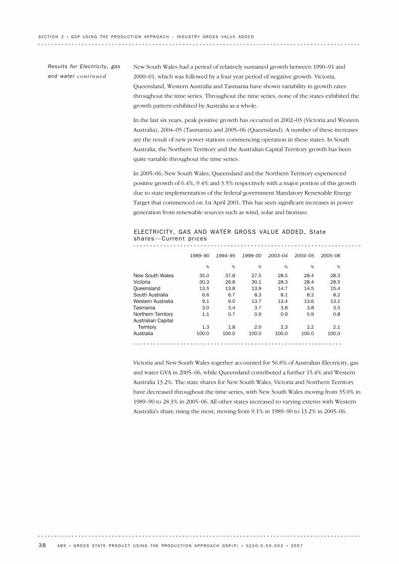
Victoria and New South Wales together accounted for 56.8% of Australian Electricity, gas
and water GVA in 2005–06, while Queensland contributed a further 15.4% and Western
Australia 13.2%. The state shares for New South Wales, Victoria and Northern Territory
have decreased throughout the time series, with New South Wales moving from 35.0% in
1989–90 to 28.3% in 2005–06. All other states increased to varying extents with Western
Australia's share rising the most, moving from 9.1% in 1989–90 to 13.2% in 2005–06.
100.0100.0100.0100.0100.0100.0Australia2.12.22.32.01.81.3
Australian CapitalTerritory
0.80.90.90.90.71.1Northern Territory3.53.83.83.73.43.0Tasmania
13.213.613.413.79.09.1Western Australia8.28.28.18.36.76.6South Australia
15.414.514.713.913.813.5Queensland28.528.428.330.126.830.3Victoria28.328.428.527.537.835.0New South Wales
%%%%%%
2005–062004–052003–041999–001994–951989–90
ELECTRIC ITY , GAS AND WATER GROSS VALUE ADDED, Stateshares —Cur ren t pr ices
New South Wales had a period of relatively sustained growth between 1990–91 and
2000–01, which was followed by a four year period of negative growth. Victoria,
Queensland, Western Australia and Tasmania have shown variability in growth rates
throughout the time series. Throughout the time series, none of the states exhibited the
growth pattern exhibited by Australia as a whole.
In the last six years, peak positive growth has occurred in 2002–03 (Victoria and Western
Australia), 2004–05 (Tasmania) and 2005–06 (Queensland). A number of these increases
are the result of new power stations commencing operation in these states. In South
Australia, the Northern Territory and the Australian Capital Territory growth has been
quite variable throughout the time series.
In 2005–06, New South Wales, Queensland and the Northern Territory experienced
positive growth of 6.4%, 9.4% and 3.5% respectively with a major portion of this growth
due to state implementation of the federal government Mandatory Renewable Energy
Target that commenced on 1st April 2001. This has seen significant increases in power
generation from renewable sources such as wind, solar and biomass.
Results for Electr ic i ty, gas
and water cont inued
38 A B S • GR O S S ST A T E P R O D U C T U S I N G T H E P R O D U C T I O N A P P R O A C H GS P ( P ) • 5 2 2 0 . 0 . 5 5 . 0 0 2 • 2 0 0 7
SE C T I O N 2 • G S P U S I N G T H E P R O D U C T I O N A P P R O A C H – I N D U S T R Y G R O S S V A L U E A D D E D

The methodology for Construction uses an output indicator approach to compile state
by industry GVA estimates. Construction output volumes are derived by the price
deflation method.
An output indicator method is used to construct volume measures of the value of work
done for residential house construction, alterations and additions to dwellings,
non-house dwelling construction, non-dwelling building and non-building
construction.The current price output estimates are sourced from the ABS, Building
Activity, Australia (BACS) (cat. no. 8752.0), and Engineering Construction Activity,
Australia (cat. no. 8762.0), at a detailed level.
The state deflators for residential house construction and alterations and additions to
dwellings are sourced from the ABS collection, House Price Index, Eight Capital Cities
(cat. no. 6416.0), specifically the state project home price index. Other dwelling price
index and non-dwelling building price indexes are sourced from the ABS PPI.
Non-building construction national deflators are constructed by the ABS using the
activity and work done, and are applied to states as no separate state level indexes are
available.
The current price and deflator data are used to derive state output volume estimates.
The output volumes are weighted together using interpolated value added data from the
ABS 1988–89 and 2002–03 Private Sector Construction Industry, Australia
(cat. no.s 8771.0 and 8772.0 respectively). The resultant estimates are then summed to
division level to derive output volume estimates.
The state output volume indicators are used to derive volume measures of GVA for
Construction. The state volume GVAs are benchmarked to the annual national industry
volume GVA.
Summary of GSP(P)
sources and methods
The Construction industry includes all units mainly engaged in constructing buildings,
roads, railroads, aerodromes, irrigation projects, harbour or river works, water, gas,
sewerage or stormwater drains or mains, electricity or other transmission lines or towers,
pipelines, oil refineries or other specified civil engineering projects. Units mainly
engaged in the repair of buildings or of other structures are also included as are those
engaged in the alteration or renovation of buildings, preparation of mine sites,
demolition and excavation.
ANZSIC Division E, Construction, consists of two sub-divisions:
! General construction (sub-division 41)
! Construction trade services (sub-division 42).
CO N S T R U C T I O N
Definit ion and scope
A B S • GR O S S ST A T E P R O D U C T U S I N G T H E P R O D U C T I O N A P P R O A C H GS P ( P ) • 5 2 2 0 . 0 . 5 5 . 0 0 2 • 2 0 0 7 39
SE C T I O N 2 • G S P U S I N G T H E P R O D U C T I O N A P P R O A C H – I N D U S T R Y G R O S S V A L U E A D D E D

(a) At basic prices.(b) Reference year for chain volume measures is 2004–05.
1990–91 1993–94 1996–97 1999–00 2002–03 2005–06
%
–20
–10
0
10
20
30AustraliaNew South WalesVictoria
CONSTRUCT ION GROSS VALUE ADDED (a) , Cha in vo lumemeasures (b )–Percentage changes
(a) At basic prices.(b) Reference year for chain volume measures is 2004–05.
8.34.86.616.411.9–13.9Australia15.03.42.420.712.6–20.3Australian Capital Territory–1.39.88.317.927.3–15.1Northern Territory12.13.317.50.224.5–10.2Tasmania23.06.13.021.813.4–13.4Western Australia
3.55.36.119.410.7–12.6South Australia10.05.18.314.710.0–11.1Queensland
5.54.18.114.613.0–12.8Victoria4.64.45.916.511.2–16.1New South Wales
PE R C E N T A G E CH A N G E S FR O M PR E V I O U S YE A R (% )
61 64456 94054 35350 97343 77739 106Australia1 4141 2291 1891 162962855Australian Capital Territory
780791720665564443Northern Territory856763739629628504Tasmania
8 2876 7406 3536 1715 0664 466Western Australia3 4753 3593 1913 0082 5202 278South Australia
12 78411 62511 06210 2158 9078 094Queensland13 24112 55012 05711 1539 7328 615Victoria20 80619 88319 04417 98415 43313 883New South Wales
VA L U E S ( $ m )
2005–062004–052003–042002–032001–022000–01
CONSTRUCT ION GROSS VALUE ADDED (a) , Cha in vo lume measures (b )Results for Construct ion
40 A B S • GR O S S ST A T E P R O D U C T U S I N G T H E P R O D U C T I O N A P P R O A C H GS P ( P ) • 5 2 2 0 . 0 . 5 5 . 0 0 2 • 2 0 0 7
SE C T I O N 2 • G S P U S I N G T H E P R O D U C T I O N A P P R O A C H – I N D U S T R Y G R O S S V A L U E A D D E D

Construction industry growth rates for the states have generally followed that of
Australia, except for Tasmania, since 2002–03. Reflecting continuous positive growth in
the national level of Construction value added since 2001–02, all states, except for the
Northern Territory, recorded positive value added growth in 2005–06.
(a) At basic prices.(b) Reference year for chain volume measures is 2004–05.
1990–91 1993–94 1996–97 1999–00 2002–03 2005–06
%
–20
–10
0
10
20
30AustraliaNorthern TerritoryAustralian Capital Territory
CONSTRUCT ION GROSS VALUE ADDED (a) , Cha in vo lumemeasures (b )–Percentage changes
(a) At basic prices.(b) Reference year for chain volume measures is 2004–05.
1990–91 1993–94 1996–97 1999–00 2002–03 2005–06
%
–20
–10
0
10
20
30AustraliaWestern AustraliaTasmania
CONSTRUCT ION GROSS VALUE ADDED (a) , Cha in vo lumemeasures (b )–Percentage changes
(a) At basic prices.(b) Reference year for chain volume measures is 2004–05.
1990–91 1993–94 1996–97 1999–00 2002–03 2005–06
%
–20
–10
0
10
20
30AustraliaQueenslandSouth Australia
CONSTRUCT ION GROSS VALUE ADDED (a) , Cha in vo lumemeasures (b )–Percentage changes
Results for Construct ion
cont inue d
A B S • GR O S S ST A T E P R O D U C T U S I N G T H E P R O D U C T I O N A P P R O A C H GS P ( P ) • 5 2 2 0 . 0 . 5 5 . 0 0 2 • 2 0 0 7 41
SE C T I O N 2 • G S P U S I N G T H E P R O D U C T I O N A P P R O A C H – I N D U S T R Y G R O S S V A L U E A D D E D

New South Wales, Victoria and Queensland together accounted for around 75% of
Australian Construction GVA in 2005–06. From 1989–90 to 2005–06, New South Wales
share fell from 33.0% to 31.8%, although during this time its share peaked in 1999–2000
at 36.7%. Victoria fell from 25.5% in 1989–90 to 21.9% in 2005–06. Queensland, Western
Australia and the Australian Capital Territory have had increased shares while the
Tasmanian and Northern Territory shares have remained relatively stable.
100.0100.0100.0100.0100.0100.0Australia2.32.22.12.32.21.8
Australian CapitalTerritory
1.31.41.41.11.21.2Northern Territory1.41.31.31.22.11.8Tasmania
14.311.811.512.012.411.5Western Australia5.45.95.96.06.67.5South Australia
21.520.420.219.219.217.8Queensland21.922.022.421.520.725.5Victoria31.834.935.236.735.533.0New South Wales
%%%%%%
2005–062004–052003–041999–001994–951989–90
CONSTRUCT ION GROSS VALUE ADDED, State shares —Curren t pr i ces
A large amount of construction work was brought forward into 1999–2000 preceding the
introduction of the GST. This resulted in a large decline in the Construction industry
across all states in 2000–01. This was followed by two years of strong growth across all
states except Tasmania, which only increased by 0.2% in 2002–03. The unusual growth in
Tasmania in 2001–02 and 2003–04 compared to other states and Australia is due to the
Devonport natural gas pipeline project which strongly increased the building and
engineering construction in these years. In 2005–06, Western Australia (23.0%), the
Australian Capital Territory (15.0%), Tasmania (12.1%), and Queensland (10.0%) all had
growth rates above the national growth of 8.3%.
Results for Construct ion
cont inue d
42 A B S • GR O S S ST A T E P R O D U C T U S I N G T H E P R O D U C T I O N A P P R O A C H GS P ( P ) • 5 2 2 0 . 0 . 5 5 . 0 0 2 • 2 0 0 7
SE C T I O N 2 • G S P U S I N G T H E P R O D U C T I O N A P P R O A C H – I N D U S T R Y G R O S S V A L U E A D D E D

The methodology for Wholesale trade uses an output indicator approach to compile
state by industry GVA estimates. Output volumes are derived by deflating total Wholesale
trade output by state at a division level. The output volumes then form the basis upon
which volume measures of value added are derived at the division level.
The current price estimates of Wholesale trade output are obtained from QBIS. Since
QBIS data are only available from 2000–01, Retail sales output (turnover) from ABS Retail
Trade, Australia (cat. no. 8501.0) has been used as a proxy to compile historical
estimates. Quarterly state output estimates are summed to derive annual output
estimates.
The current price output estimates are priced deflated using the national Wholesale
trade deflator from 2000–01. Prior to that, the Retail trade deflator by state is used.
The state output indicators are used to derive volume measures of GVA for Wholesale
Trade. The state volume GVAs are benchmarked to the annual national industry volume
GVA.
Summary of GSP(P)
sources and methods
The Wholesale trade industry includes those units mainly engaged in the resale (as
agents or principals) of new or used goods to businesses or to institutional (including
Government) users.
ANZSIC Division F, Wholesale trade, consists of three sub-divisions:
! Basic material wholesaling (sub-division 45)
! Machinery and motor vehicle wholesaling (sub-division 46)
! Personal and household good wholesaling (sub-division 47).
WH O L E S A L E TR A D E
Definit ion and scope
A B S • GR O S S ST A T E P R O D U C T U S I N G T H E P R O D U C T I O N A P P R O A C H GS P ( P ) • 5 2 2 0 . 0 . 5 5 . 0 0 2 • 2 0 0 7 43
SE C T I O N 2 • G S P U S I N G T H E P R O D U C T I O N A P P R O A C H – I N D U S T R Y G R O S S V A L U E A D D E D

(a) At basic prices.(b) Reference year for chain volume measures is 2004–05.
1990–91 1993–94 1996–97 1999–00 2002–03 2005–06
%
–20
–10
0
10
20
30AustraliaNew South WalesVictoria
WHOLESALE TRADE GROSS VALUE ADDED (a) , Cha in vo lumemeasures (b )–Percentage changes
(a) At basic prices.(b) Reference year for chain volume measures is 2004–05.
2.93.44.84.82.7–0.4Australia2.010.31.1–0.8–3.814.1Australian Capital Territory
25.9–0.5–6.68.8–5.8–14.1Northern Territory9.76.54.59.3–8.9–11.1Tasmania
17.94.714.56.88.26.4Western Australia2.00.94.43.113.5–5.7South Australia4.04.15.00.98.77.0Queensland
–0.91.811.015.60.2–5.3Victoria0.54.0–2.5–1.70.7–0.6New South Wales
PE R C E N T A G E CH A N G E S FR O M PR E V I O U S YE A R (% )
44 88643 62542 17440 26038 43337 435Australia352345313309312324Australian Capital Territory292232233250229243Northern Territory611557523500458503Tasmania
4 8154 0833 8993 4073 1902 949Western Australia2 5282 4802 4582 3542 2852 013South Australia8 1017 7937 4887 1317 0696 504Queensland
12 17112 27612 05710 8589 3909 371Victoria15 93915 85915 25015 63715 91115 806New South Wales
VA L U E S ( $ m )
2005–062004–052003–042002–032001–022000–01
WHOLESALE TRADE GROSS VALUE ADDED (a) , Cha in vo lumemeasures (b )
Results for Wholesale
trade
44 A B S • GR O S S ST A T E P R O D U C T U S I N G T H E P R O D U C T I O N A P P R O A C H GS P ( P ) • 5 2 2 0 . 0 . 5 5 . 0 0 2 • 2 0 0 7
SE C T I O N 2 • G S P U S I N G T H E P R O D U C T I O N A P P R O A C H – I N D U S T R Y G R O S S V A L U E A D D E D

From 2002–03 to 2004–05, most states exhibited positive growth rates of varying degrees
except for New South Wales, the Northern Territory and the Australian Capital Territory.
In 2005–06, Victoria had negative growth whereas all other states had positive growth.
Western Australia and the Northern Territory recorded growth rates of 17.9% and 25.9%
(a) At basic prices.(b) Reference year for chain volume measures is 2004–05.
1990–91 1993–94 1996–97 1999–00 2002–03 2005–06
%
–20
–10
0
10
20
30AustraliaNorthern TerritoryAustralian Capital Territory
WHOLESALE TRADE GROSS VALUE ADDED (a) , Cha in vo lumemeasures (b )–Percentage changes
(a) At basic prices.(b) Reference year for chain volume measures is 2004–05.
1990–91 1993–94 1996–97 1999–00 2002–03 2005–06
%
–20
–10
0
10
20
30AustraliaWestern AustraliaTasmania
WHOLESALE TRADE GROSS VALUE ADDED (a) , Cha in vo lumemeasures (b )–Percentage changes
(a) At basic prices.(b) Reference year for chain volume measures is 2004–05.
1990–91 1993–94 1996–97 1999–00 2002–03 2005–06
%
–20
–10
0
10
20
30AustraliaQueenslandSouth Australia
WHOLESALE TRADE GROSS VALUE ADDED (a) , Cha in vo lumemeasures (b )–Percentage changes
Results for Wholesale
trade cont inue d
A B S • GR O S S ST A T E P R O D U C T U S I N G T H E P R O D U C T I O N A P P R O A C H GS P ( P ) • 5 2 2 0 . 0 . 5 5 . 0 0 2 • 2 0 0 7 45
SE C T I O N 2 • G S P U S I N G T H E P R O D U C T I O N A P P R O A C H – I N D U S T R Y G R O S S V A L U E A D D E D

The three largest states, New South Wales, Victoria and Queensland, accounted for over
80% of Australian Wholesale trade GVA in 2005–06. The state shares have been fairly
stable throughout the time series.
100.0100.0100.0100.0100.0100.0Australia0.80.80.80.90.81.0
Australian CapitalTerritory
0.50.50.50.60.60.6Northern Territory1.31.31.31.31.61.6Tasmania9.39.49.38.710.38.7Western Australia5.65.75.75.96.26.6South Australia
17.817.917.817.115.614.8Queensland28.828.128.227.526.729.7Victoria35.836.436.638.138.137.1New South Wales
%%%%%%
2005–062004–052003–041999–001994–951989–90
WHOLESALE TRADE GROSS VALUE ADDED, State shares —Curren tpr ices
respectively which reflected the strong demand for commodities in mining and industrial
materials in these states.
Results for Wholesale
trade cont inue d
46 A B S • GR O S S ST A T E P R O D U C T U S I N G T H E P R O D U C T I O N A P P R O A C H GS P ( P ) • 5 2 2 0 . 0 . 5 5 . 0 0 2 • 2 0 0 7
SE C T I O N 2 • G S P U S I N G T H E P R O D U C T I O N A P P R O A C H – I N D U S T R Y G R O S S V A L U E A D D E D
The methodology for Retail trade uses an output indicator approach to compile state by
industry GVA estimates. Output volumes are derived by deflating total Retail Trade
output by state at a division level, except for new car sales which are quantity revalued.
The output volumes then form the basis upon which volume measures of value added
are derived at the division level.
Current price turnover data is sourced from ABS Retail Trade, Australia (cat. no. 8501.0)
and current price Household final consumption expenditure (HFCE) data for
consumption outside the scope of Retail Trade, Australia. Price information is sourced
from the CPI and used to deflate the current price turnover data to derive a set of
turnover volume measures.
For new car sales the quantity indicator is sourced from VFACTS which contains national
statistics for sales of new motor vehicles, produced and published on a monthly basis by
the Federal Chamber of Automotive Industries.
The volume output measures are weighted together using class level GVA weights to
obtain the division GVA volume output measure. The class level GVA weights are derived
by multiplying current price turnover data by annual value added to turnover ratios
derived from the current price data in the ABS 1998–99 Retail Census and Economy Wide
Surveys.
The state output indicators are used to derive volume measures of GVA for Retail trade.
The state volume GVAs are benchmarked to the annual national industry volume GVA.
Summary of GSP(P)
sources and methods
The Retail trade industry includes all units mainly engaged in the resale (as agents or
principals) of new or used goods to final consumers for personal or household
consumption or in selected repair activities such as repair of household equipment or
motor vehicles.
ANZSIC Division G, Retail trade, consists of three sub-divisions:
! Food retailing (sub-division 51)
! Personal and household good retailing (sub-division 52)
! Motor vehicle retailing and services (sub-division 53).
RE T A I L TR A D E
Definit ion and scope
A B S • GR O S S ST A T E P R O D U C T U S I N G T H E P R O D U C T I O N A P P R O A C H GS P ( P ) • 5 2 2 0 . 0 . 5 5 . 0 0 2 • 2 0 0 7 47
SE C T I O N 2 • G S P U S I N G T H E P R O D U C T I O N A P P R O A C H – I N D U S T R Y G R O S S V A L U E A D D E D

(a) At basic prices.(b) Reference year for chain volume measures is 2004–05.
1990–91 1993–94 1996–97 1999–00 2002–03 2005–06
%
–20
–10
0
10
20
30AustraliaNew South WalesVictoria
RETA IL TRADE GROSS VALUE ADDED (a) , Cha in vo lumemeasures (b )–Percentage changes
— nil or rounded to zero (including null cells)(a) At basic prices.(b) Reference year for chain volume measures is 2004–05.
1.04.35.24.65.21.8Australia3.01.81.81.45.57.0Australian Capital Territory
–0.62.54.12.94.4–0.1Northern Territory6.15.28.53.03.12.9Tasmania4.07.25.52.15.21.1Western Australia
–0.13.91.14.67.23.0South Australia1.25.29.46.44.72.7Queensland0.75.34.64.67.01.4Victoria—2.43.74.74.01.3New South Wales
PE R C E N T A G E CH A N G E S FR O M PR E V I O U S YE A R (% )
53 24252 72050 52548 04845 92143 646Australia928901884869857812Australian Capital Territory493496484465452433Northern Territory
1 1911 1231 067983954925Tasmania5 4845 2714 9184 6644 5694 344Western Australia3 4293 4323 3023 2683 1242 914South Australia
11 75011 61311 03810 0909 4879 064Queensland12 82812 74012 09911 57011 06610 345Victoria17 13917 14516 74116 14215 41314 815New South Wales
VA L U E S ( $ m )
2005–062004–052003–042002–032001–022000–01
RETAIL TRADE GROSS VALUE ADDED (a) , Cha in vo lume measures (b )Results for Retai l trade
48 A B S • GR O S S ST A T E P R O D U C T U S I N G T H E P R O D U C T I O N A P P R O A C H GS P ( P ) • 5 2 2 0 . 0 . 5 5 . 0 0 2 • 2 0 0 7
SE C T I O N 2 • G S P U S I N G T H E P R O D U C T I O N A P P R O A C H – I N D U S T R Y G R O S S V A L U E A D D E D

(a) At basic prices.(b) Reference year for chain volume measures is 2004–05.
1990–91 1993–94 1996–97 1999–00 2002–03 2005–06
%
–20
–10
0
10
20
30AustraliaNorthern TerritoryAustralian Capital Territory
RETA IL TRADE GROSS VALUE ADDED (a) , Cha in vo lumemeasures (b )–Percentage changes
(a) At basic prices.(b) Reference year for chain volume measures is 2004–05.
1990–91 1993–94 1996–97 1999–00 2002–03 2005–06
%
–20
–10
0
10
20
30AustraliaWestern AustraliaTasmania
RETAIL TRADE GROSS VALUE ADDED (a) , Cha in vo lumemeasures (b )–Percentage changes
(a) At basic prices.(b) Reference year for chain volume measures is 2004–05.
1990–91 1993–94 1996–97 1999–00 2002–03 2005–06
%
–20
–10
0
10
20
30AustraliaQueenslandSouth Australia
RETA IL TRADE GROSS VALUE ADDED (a) , Cha in vo lumemeasures (b )–Percentage changes
Results for Retai l trade
cont inue d
A B S • GR O S S ST A T E P R O D U C T U S I N G T H E P R O D U C T I O N A P P R O A C H GS P ( P ) • 5 2 2 0 . 0 . 5 5 . 0 0 2 • 2 0 0 7 49
SE C T I O N 2 • G S P U S I N G T H E P R O D U C T I O N A P P R O A C H – I N D U S T R Y G R O S S V A L U E A D D E D

New South Wales, Victoria and Queensland together accounted for 78.6% of Australian
Retail trade value added in 2005–06. New South Wales, Victoria and South Australia's
shares decreased slightly throughout the time series whereas shares in Tasmania, the
Northern Territory and the Australian Capital Territory were quite stable. Western
Australia's share increased from 8.9% in 1989–90 to 10.1% in 1994–95 and has stabilised
around that level. Queensland gradually increased its share throughout the time series
from 17.2% in 1989–90 to 22.6% in 2005–06.
100.0100.0100.0100.0100.0100.0Australia1.71.71.81.81.81.6
Australian CapitalTerritory
1.00.90.91.01.11.1Northern Territory2.22.12.22.22.62.4Tasmania
10.010.010.110.010.18.9Western Australia6.66.56.67.27.88.2South Australia
22.622.021.420.219.117.2Queensland23.724.224.323.923.025.3Victoria32.332.532.733.834.535.2New South Wales
%%%%%%
2005–062004–052003–041999–001994–951989–90
RETAIL TRADE GROSS VALUE ADDED, State shares —Curren t pr ices
From 2001–02 to 2004–05, all states exhibited positive growth rates of varying degrees
with Queensland and Tasmania recording peak growth rates of 9.4% and 8.5%
respectively in 2003–04. In 2005–06 there was a significant slow down in growth from the
previous year for all states except Tasmania and the Australian Capital Territory, which
both increased to 6.1% and 3.0% respectively.
Results for Retai l trade
cont inue d
50 A B S • GR O S S ST A T E P R O D U C T U S I N G T H E P R O D U C T I O N A P P R O A C H GS P ( P ) • 5 2 2 0 . 0 . 5 5 . 0 0 2 • 2 0 0 7
SE C T I O N 2 • G S P U S I N G T H E P R O D U C T I O N A P P R O A C H – I N D U S T R Y G R O S S V A L U E A D D E D

The methodology for Accommodation, cafes and restaurants uses an output indicator
approach to compile state by industry GVA estimates. Output volumes are derived using
quantity revaluation for the state output of Accommodation and price deflation for Cafes
and restaurants. The output volumes then form the basis upon which volume measures
of value added are derived at the division level.
For accommodation, quantity data (guest nights) and turnover data for hotels, motels,
serviced apartments, caravan parks and holiday flats are sourced from the ABS Tourist
Accommodation, Australia (cat. no. 8635.0).
Cafes and restaurants current price estimates are sourced from the ABS publication
Retail Trade, Australia by state. Price deflators are sourced from the ABS CPI by capital
city.
The state output indicators are used to derive volume measures of GVA for
Accommodation, cafes and restaurants. The state volume GVAs are benchmarked to the
annual national industry volume GVA.
Summary of GSP(P)
sources and methods
The Accommodation, cafes and restaurants industry includes all units mainly engaged in
providing hospitality services in the form of accommodation, meals and drinks.
ANZSIC Division G, Accommodation, cafes and restaurants, consists of one sub-division:
! Accommodation, cafes and restaurants (sub-division 57).
AC C O M M O D A T I O N , CA F E S
AN D RE S T A U R A N T S
Definit ion and scope
A B S • GR O S S ST A T E P R O D U C T U S I N G T H E P R O D U C T I O N A P P R O A C H GS P ( P ) • 5 2 2 0 . 0 . 5 5 . 0 0 2 • 2 0 0 7 51
SE C T I O N 2 • G S P U S I N G T H E P R O D U C T I O N A P P R O A C H – I N D U S T R Y G R O S S V A L U E A D D E D
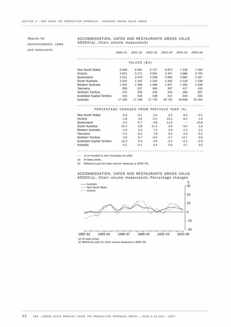
(a) At basic prices.(b) Reference year for chain volume measures is 2004–05.
1990–91 1993–94 1996–97 1999–00 2002–03 2005–06
%
–20
–10
0
10
20
30AustraliaNew South WalesVictoria
ACCOMMODATION, CAFES AND RESTAURANTS GROSS VALUEADDED (a) , Cha in vo lume measures (b )–Percentage changes
— nil or rounded to zero (including null cells)(a) At basic prices.(b) Reference year for chain volume measures is 2004–05.
3.04.75.63.4–0.14.2Australia–2.9–2.2–5.54.90.313.3Australian Capital Territory6.614.7–4.7–5.0–5.72.9Northern Territory
–0.25.09.47.8–6.2–4.5Tasmania2.4–1.02.67.45.3–1.6Western Australia1.6–3.42.611.45.810.4South Australia
10.8—11.35.8–5.75.4Queensland1.98.210.2–2.53.9–1.8Victoria
–0.58.22.22.5–0.16.3New South Wales
PE R C E N T A G E CH A N G E S FR O M PR E V I O U S YE A R (% )
20 20419 60818 73217 73517 15817 166Australia393405414438418416Australian Capital Territory287269235246259275Northern Territory416417397363337359Tasmania
1 5281 4921 5071 4691 3681 300Western Australia1 2381 2181 2621 2301 1041 043South Australia5 1874 6824 6834 2093 9794 221Queensland3 7553 6863 4073 0913 1713 051Victoria7 4007 4396 8736 7276 5626 569New South Wales
VA L U E S ( $ m )
2005–062004–052003–042002–032001–022000–01
ACCOMMODATION, CAFES AND RESTAURANTS GROSS VALUEADDED (a) , Cha in vo lume measures (b )
Results for
Accommodation, cafes
and restaurants
52 A B S • GR O S S ST A T E P R O D U C T U S I N G T H E P R O D U C T I O N A P P R O A C H GS P ( P ) • 5 2 2 0 . 0 . 5 5 . 0 0 2 • 2 0 0 7
SE C T I O N 2 • G S P U S I N G T H E P R O D U C T I O N A P P R O A C H – I N D U S T R Y G R O S S V A L U E A D D E D

New South Wales had a long period of growth from 1993–94 to 2004–05 with only one
year of minor negative growth in 2001–02. Victoria experienced strong growth in the late
1990's followed by a period of low or negative growth. Queensland has shown continual
growth throughout the time series, with only one year of negative growth in 2001–02.
(a) At basic prices.(b) Reference year for chain volume measures is 2004–05.
1990–91 1993–94 1996–97 1999–00 2002–03 2005–06
%
–20
–10
0
10
20
30AustraliaNorthern TerritoryAustralian Capital Territory
ACCOMMODATION, CAFES AND RESTAURANTS GROSS VALUEADDED (a) , Cha in vo lume measures (b )–Percentage changes
(a) At basic prices.(b) Reference year for chain volume measures is 2004–05.
1990–91 1993–94 1996–97 1999–00 2002–03 2005–06
%
–20
–10
0
10
20
30AustraliaWestern AustraliaTasmania
ACCOMMODATION, CAFES AND RESTAURANTS GROSS VALUEADDED (a) , Cha in vo lume measures (b )–Percentage changes
(a) At basic prices.(b) Reference year for chain volume measures is 2004–05.
1990–91 1993–94 1996–97 1999–00 2002–03 2005–06
%
–20
–10
0
10
20
30AustraliaQueenslandSouth Australia
ACCOMMODATION, CAFES AND RESTAURANTS GROSS VALUEADDED (a) , Cha in vo lume measures (b )–Percentage changes
Results for
Accommodation, cafes
and restaurants
cont inue d
A B S • GR O S S ST A T E P R O D U C T U S I N G T H E P R O D U C T I O N A P P R O A C H GS P ( P ) • 5 2 2 0 . 0 . 5 5 . 0 0 2 • 2 0 0 7 53
SE C T I O N 2 • G S P U S I N G T H E P R O D U C T I O N A P P R O A C H – I N D U S T R Y G R O S S V A L U E A D D E D

The share for New South Wales has decreased over the time series from 42.1% in
1989–90 to 36.9% in 2005–06. Queensland has been the main state to increase its share,
rising from 19.7% in 1989–90 to 24.7% in 2005–06.
100.0100.0100.0100.0100.0100.0Australia1.92.12.21.91.91.6
Australian CapitalTerritory
1.51.41.41.51.51.3Northern Territory2.12.12.12.02.42.2Tasmania7.87.67.67.77.37.7Western Australia6.46.26.36.76.27.5South Australia
24.723.923.022.221.619.7Queensland18.718.818.518.118.418.1Victoria36.937.938.839.940.742.1New South Wales
%%%%%%
2005–062004–052003–041999–001994–951989–90
ACCOMMODATION, CAFES AND RESTAURANTS GROSS VALUE ADDED,State shares —Curren t pr ices
South Australia and Tasmania experienced strong growth in 1993–94 and 1994–95 which
coincided with the introduction of gaming machines in clubs and hotels in these states.
Western Australia and the Northern Territory maintained continuous growth between
1989–90 and 1998–99. The Australian Capital Territory's growth rate has been variable
throughout the time series, with the latest three years all showing negative growth. In
2005–06, all states had positive growth except New South Wales, Tasmania and the
Australian Capital Territory. Queensland and the Northern Territory were the only states
to have growth above the national growth of 3.0%, at 10.8% and 6.6% respectively.
Results for
Accommodation, cafes
and restaurants
cont inue d
54 A B S • GR O S S ST A T E P R O D U C T U S I N G T H E P R O D U C T I O N A P P R O A C H GS P ( P ) • 5 2 2 0 . 0 . 5 5 . 0 0 2 • 2 0 0 7
SE C T I O N 2 • G S P U S I N G T H E P R O D U C T I O N A P P R O A C H – I N D U S T R Y G R O S S V A L U E A D D E D
The methodology for Transport and storage uses an output indicator approach to
compile state by industry GVA estimates. Output volumes are derived by either price
deflation or quantity revaluation. These output volumes then form the basis upon which
volume measures of value added are derived at the division level.
Output indicators are drawn from a number of different sources for each sub-division.
! For road freight the quantity indicator is 'tonne/kilometres' from the Survey of Motor
Vehicle Use, Data Cubes, Australia (cat. no. 9210.0.55.001).
! For road passenger transport HFCE estimates are deflated by CPI components by
capital city.
! For public passenger rail transport HFCE estimates are price deflated by CPI
components by capital city.
! For private rail transport QBIS turnover estimates are price deflated using national
level price indexes from PPI as no separate state level indexes are available.
! For water transport the quantity indicator is 'kilotonnes loaded and unloaded' from
the Bureau of Transport and Regional Economics (BTRE) publication Australian Sea
Freight.
! For air transport data the quantity indicator is 'passenger numbers' at major airports
from the BTRE Airport Traffic publication.
! For other transport, services to transport and storage QBIS turnover estimates are
price deflated using national level price indexes from PPI as no separate state level
indexes are available.
For those sub-divisions that include QBIS as an indicator, the total hours worked by state
for each sub-division from the Labour Force, Australia, Detailed, Quarterly
(cat. no. 6291.0.55.003) has been used to extrapolate back the state estimates prior to
2000–01.
The state output indicators for each sub-division are then summed together to produce a
total for the Transport and storage industry. This total output indicator is used to derive
volume measures to derive state GVA for Transport and storage.
The state volume GVAs are benchmarked to the annual national industry volume GVA.
Summary of GSP(P)
sources and methods
The Transport and storage industry includes all units mainly engaged in passenger or
freight transport by road, rail, water or air; terminal facilities of passengers or freight;
services related to transport such as car parking, stevedoring, harbour services,
navigation services, airport operation or space port operation; booking, travel, freight
forwarding, crating and customs agency services; and storage facilities.
ANZSIC Division I, Transport and storage, consists of seven sub-divisions:
! Road transport (sub-division 61)
! Rail transport (sub-division 62)
! Water transport (sub-division 63)
! Air and space transport (sub-division 64)
! Other transport (sub-division 65)
! Services to transport (sub-division 66)
! Storage (sub-division 67).
TR A N S P O R T AN D
ST O R A G E
Definit ion and scope
A B S • GR O S S ST A T E P R O D U C T U S I N G T H E P R O D U C T I O N A P P R O A C H GS P ( P ) • 5 2 2 0 . 0 . 5 5 . 0 0 2 • 2 0 0 7 55
SE C T I O N 2 • G S P U S I N G T H E P R O D U C T I O N A P P R O A C H – I N D U S T R Y G R O S S V A L U E A D D E D

(a) At basic prices.(b) Reference year for chain volume measures is 2004–05.
1990–91 1993–94 1996–97 1999–00 2002–03 2005–06
%
–20
–10
0
10
20
30AustraliaNew South WalesVictoria
TRANSPORT AND STORAGE GROSS VALUE ADDED (a) , Cha in vo lumemeasures (b )–Percentage changes
(a) At basic prices.(b) Reference year for chain volume measures is 2004–05.
2.65.04.47.03.64.3Australia6.13.95.9–3.2–0.31.3Australian Capital Territory5.212.27.5–1.9–1.62.3Northern Territory2.8–0.611.29.85.47.5Tasmania6.90.27.011.55.34.7Western Australia
–1.61.57.78.62.62.5South Australia3.56.46.12.16.86.8Queensland1.87.92.111.91.67.6Victoria1.74.72.85.23.20.9New South Wales
PE R C E N T A G E CH A N G E S FR O M PR E V I O U S YE A R (% )
42 03740 96639 02837 38534 94733 717Australia501472454429443445Australian Capital Territory503478426396404410Northern Territory799777782704641608Tasmania
5 4175 0655 0534 7224 2344 023Western Australia2 8632 9102 8662 6612 4502 388South Australia8 7388 4437 9327 4767 3256 858Queensland9 4949 3238 6408 4647 5667 449Victoria
13 72213 49812 89412 54411 92411 556New South Wales
VA L U E S ( $ m )
2005–062004–052003–042002–032001–022000–01
TRANSPORT AND STORAGE GROSS VALUE ADDED (a) , Cha in vo lumemeasures (b )
Results for Transport and
storage
56 A B S • GR O S S ST A T E P R O D U C T U S I N G T H E P R O D U C T I O N A P P R O A C H GS P ( P ) • 5 2 2 0 . 0 . 5 5 . 0 0 2 • 2 0 0 7
SE C T I O N 2 • G S P U S I N G T H E P R O D U C T I O N A P P R O A C H – I N D U S T R Y G R O S S V A L U E A D D E D

(a) At basic prices.(b) Reference year for chain volume measures is 2004–05.
1990–91 1993–94 1996–97 1999–00 2002–03 2005–06
%
–20
–10
0
10
20
30AustraliaNorthern TerritoryAustralian Capital Territory
TRANSPORT AND STORAGE GROSS VALUE ADDED (a) , Cha in vo lumemeasures (b )–Percentage changes
(a) At basic prices.(b) Reference year for chain volume measures is 2004–05.
1990–91 1993–94 1996–97 1999–00 2002–03 2005–06
%
–20
–10
0
10
20
30AustraliaWestern AustraliaTasmania
TRANSPORT AND STORAGE GROSS VALUE ADDED (a) , Cha in vo lumemeasures (b )–Percentage changes
(a) At basic prices.(b) Reference year for chain volume measures is 2004–05.
1990–91 1993–94 1996–97 1999–00 2002–03 2005–06
%
–20
–10
0
10
20
30AustraliaQueenslandSouth Australia
TRANSPORT AND STORAGE GROSS VALUE ADDED (a) , Cha in vo lumemeasures (b )–Percentage changes
Results for Transport and
storage cont inu ed
A B S • GR O S S ST A T E P R O D U C T U S I N G T H E P R O D U C T I O N A P P R O A C H GS P ( P ) • 5 2 2 0 . 0 . 5 5 . 0 0 2 • 2 0 0 7 57
SE C T I O N 2 • G S P U S I N G T H E P R O D U C T I O N A P P R O A C H – I N D U S T R Y G R O S S V A L U E A D D E D

New South Wales, Victoria and Queensland together accounted for around 77% of
Australian Transport and storage GVA in 2005–06. Most state shares for the Transport
and storage industry have been fairly stable throughout the time series, although New
South Wales lost share from 36.8% in 1989–90 to 32.9% in 2005–06, Queensland
increased its share from 18.5% in 1989–90 to 20.8% in 2005–06 and Western Australia
increased from 10.0% in 1989–90 to 12.3% in 2005–06.
100.0100.0100.0100.0100.0100.0Australia1.11.21.11.31.41.6
Australian CapitalTerritory
1.11.21.11.11.00.9Northern Territory1.81.91.81.61.82.1Tasmania
12.312.412.512.110.010.0Western Australia6.67.16.86.17.27.0South Australia
20.820.620.519.120.018.5Queensland23.522.822.223.321.923.2Victoria32.932.933.935.436.736.8New South Wales
%%%%%%
2005–062004–052003–041999–001994–951989–90
TRANSPORT AND STORAGE GROSS VALUE ADDED, Stateshares —Cur ren t pr ices
Queensland has shown growth throughout the whole of the time series. Western
Australia has grown in all years except 1999–2000 when there was a small fall. In 2005–06,
South Australia was the only state to show negative growth of –1.6%. All other states had
growth rates higher than the national rate of 2.6% except for New South Wales and
Victoria.
Results for Transport and
storage cont inu ed
58 A B S • GR O S S ST A T E P R O D U C T U S I N G T H E P R O D U C T I O N A P P R O A C H GS P ( P ) • 5 2 2 0 . 0 . 5 5 . 0 0 2 • 2 0 0 7
SE C T I O N 2 • G S P U S I N G T H E P R O D U C T I O N A P P R O A C H – I N D U S T R Y G R O S S V A L U E A D D E D

The methodology for Communication services uses an output indicator approach to
compile state by industry GVA estimates. Turnover volume measures are estimated using
revenue data and price indexes from the ABS CPI. The output volumes then form the
basis upon which volume measures of value added are derived at the division level.
For postage services, state revenue data from Australia Post (2000–01 onwards) and
private postal and courier turnover data from QBIS (2001–02 onwards) is used. Australia
Post revenue has been extrapolated back to 1989–90 based on state population
estimates. State private postal and courier revenue has been extrapolated back based on
national private postal and courier revenue.
Estimates of public telecommunications services are based on national revenue data for
Telstra and has been split to state using population data. State private
telecommunication revenue data are available from QBIS for each state back to 2001-02.
The state private telecommunication revenue has been backcast based on national
private telecommunication revenue.
The output indicators are price deflated to produce state turnover volume measures.
Australia Post and private postal and courier current price turnover are both deflated
using the ABS CPI postal services data for the eight capital cities. The Telstra and private
telecommunication turnover are deflated using the ABS CPI telecommunication services
data for the eight capital cities.
These state turnover volume measures are aggregated and used to produce volume
measures of GVA for state Communication services. The state volume GVAs are
benchmarked to the annual national industry volume GVA.
Summary of GSP(P)
sources and methods
The Communication services industry includes all units mainly engaged in providing
postal, courier and telecommunication services.
ANZSIC93 Division J, Communication services, consists of one sub-division:
! Communication services (sub-division 71).
This sub-division is made up of two groups:
! Postal and courier services (group 711)
! Telecommunication services (group 712).
CO M M U N I C A T I O N
SE R V I C E S
Definit ion and scope
A B S • GR O S S ST A T E P R O D U C T U S I N G T H E P R O D U C T I O N A P P R O A C H GS P ( P ) • 5 2 2 0 . 0 . 5 5 . 0 0 2 • 2 0 0 7 59
SE C T I O N 2 • G S P U S I N G T H E P R O D U C T I O N A P P R O A C H – I N D U S T R Y G R O S S V A L U E A D D E D
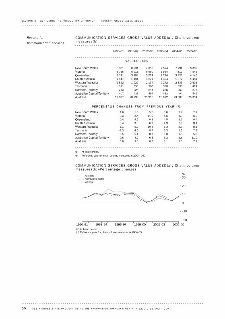
(a) At basic prices.(b) Reference year for chain volume measures is 2004–05.
1990–91 1993–94 1996–97 1999–00 2002–03 2005–06
%
–20
–10
0
10
20
30AustraliaNew South WalesVictoria
COMMUNICAT ION SERVICES GROSS VALUE ADDED (a) , Cha in vo lumemeasures (b )–Percentage changes
(a) At basic prices.(b) Reference year for chain volume measures is 2004–05.
7.42.55.18.33.00.8Australia11.02.56.36.34.90.6Australian Capital Territory
5.31.85.08.75.10.5Northern Territory7.31.26.38.74.5–1.3Tasmania8.12.76.310.85.91.1Western Australia8.12.94.96.73.80.4South Australia8.42.54.58.84.50.4Queensland6.01.96.511.02.50.3Victoria7.72.93.65.51.61.6New South Wales
PE R C E N T A G E CH A N G E S FR O M PR E V I O U S YE A R (% )
25 33123 58823 02221 91520 23019 637Australia549494482454427407Australian Capital Territory274260256244224213Northern Territory421393388365336321Tasmania
2 5212 3332 2722 1371 9291 822Western Australia1 4841 3721 3341 2711 1911 147South Australia4 1463 8263 7343 5743 2843 141Queensland7 5487 1196 9846 5605 9115 765Victoria8 3897 7917 5747 3106 9316 821New South Wales
VA L U E S ( $ m )
2005–062004–052003–042002–032001–022000–01
COMMUNICAT ION SERVICES GROSS VALUE ADDED (a) , Cha in vo lumemeasures (b )
Results for
Communicat ion serv ices
60 A B S • GR O S S ST A T E P R O D U C T U S I N G T H E P R O D U C T I O N A P P R O A C H GS P ( P ) • 5 2 2 0 . 0 . 5 5 . 0 0 2 • 2 0 0 7
SE C T I O N 2 • G S P U S I N G T H E P R O D U C T I O N A P P R O A C H – I N D U S T R Y G R O S S V A L U E A D D E D

(a) At basic prices.(b) Reference year for chain volume measures is 2004–05.
1990–91 1993–94 1996–97 1999–00 2002–03 2005–06
%
–20
–10
0
10
20
30AustraliaNorthern TerritoryAustralian Capital Territory
COMMUNICAT ION SERVICES GROSS VALUE ADDED (a) , Cha in vo lumemeasures (b )–Percentage changes
(a) At basic prices.(b) Reference year for chain volume measures is 2004–05.
1990–91 1993–94 1996–97 1999–00 2002–03 2005–06
%
–20
–10
0
10
20
30AustraliaWestern AustraliaTasmania
COMMUNICAT ION SERVICES GROSS VALUE ADDED (a) , Cha in vo lumemeasures (b )–Percentage changes
(a) At basic prices.(b) Reference year for chain volume measures is 2004–05.
1990–91 1993–94 1996–97 1999–00 2002–03 2005–06
%
–20
–10
0
10
20
30AustraliaQueenslandSouth Australia
COMMUNICAT ION SERVICES GROSS VALUE ADDED (a) , Cha in vo lumemeasures (b )–Percentage changes
Results for
Communicat ion serv ices
cont inue d
A B S • GR O S S ST A T E P R O D U C T U S I N G T H E P R O D U C T I O N A P P R O A C H GS P ( P ) • 5 2 2 0 . 0 . 5 5 . 0 0 2 • 2 0 0 7 61
SE C T I O N 2 • G S P U S I N G T H E P R O D U C T I O N A P P R O A C H – I N D U S T R Y G R O S S V A L U E A D D E D

New South Wales and Victoria together accounted for over 63% of Australian
Communication services GVA in 2005–06. New South Wales, South Australia and
Tasmania have decreased their shares over the time series, with New South Wales
declining from 37.1% in 1989–90 to 33.0% in 2005–06. Victoria, Queensland, Western
Australia and the Australian Capital Territory all increased their share. Victoria increased
its share from 27.3% in 1989–90 to 30.3% in 2005–06.
100.0100.0100.0100.0100.0100.0Australia2.02.12.01.82.11.6
Australian CapitalTerritory
1.11.11.11.21.10.9Northern Territory1.61.71.61.71.71.8Tasmania9.89.910.010.09.99.1Western Australia6.05.86.06.06.37.1South Australia
16.116.216.416.416.515.2Queensland30.330.229.628.128.527.3Victoria33.033.033.434.833.937.1New South Wales
%%%%%%
2005–062004–052003–041999–001994–951989–90
COMMUNICAT ION SERVICES GROSS VALUE ADDED, Stateshares —Cur ren t pr ices
New South Wales, Tasmania and the Northern Territory diverged slightly from the
Australian growth pattern during the 1990s. From 2001–02, all states increased their
growth, with quite large growth in 2002–03, especially in Victoria (11.0%) and Western
Australia (10.8%). In 2005–06, all states experienced high growth ranging from 5.3% in
the Northern Territory to 11.0% in the Australian Capital Territory.
Results for
Communicat ion serv ices
cont inue d
62 A B S • GR O S S ST A T E P R O D U C T U S I N G T H E P R O D U C T I O N A P P R O A C H GS P ( P ) • 5 2 2 0 . 0 . 5 5 . 0 0 2 • 2 0 0 7
SE C T I O N 2 • G S P U S I N G T H E P R O D U C T I O N A P P R O A C H – I N D U S T R Y G R O S S V A L U E A D D E D

The methodology for Finance and insurance uses an output indicator approach to
compile national GVA estimates. The output volumes then form the basis upon which
volume measures of value added are derived at the division level.
Component national current price and volume data are collected at the industry
sub-division level. These are sourced from the Australian Prudential Regulatory Authority
(APRA) for Finance and Insurance and from the Economic Activity Survey for Services to
finance and insurance.
These national data are allocated to state using hours worked, by state, by industry group
from the ABS Labour Force, Australia. Both current price and volume measure output
values are split by state and by industry sub-division.
Industry sub-division volume output data are then summed to derive a total for the
industry which is then chained to compile the state volume output.
These state output indicators are used to derive volume measures of GVA for Finance
and insurance. The state volume GVAs are benchmarked to the annual national industry
volume GVA.
Summary of GSP(P)
sources and methods
The Finance and insurance industry includes all units mainly engaged in the provision of
finance, in investing money in predominantly financial assets, in providing services to
lenders, borrowers and investors, in providing insurance cover of all types, and in
providing services to insurance underwriters and to people or organisations seeking
insurance.
ANZSIC Division K, Finance and insurance, consists of three sub-divisions:
! Finance (sub-division 73)
! Insurance (sub-division 74)
! Services to finance and insurance (sub-division 75).
F I N A N C E AN D IN S U R A N C E
Definit ion and scope
A B S • GR O S S ST A T E P R O D U C T U S I N G T H E P R O D U C T I O N A P P R O A C H GS P ( P ) • 5 2 2 0 . 0 . 5 5 . 0 0 2 • 2 0 0 7 63
SE C T I O N 2 • G S P U S I N G T H E P R O D U C T I O N A P P R O A C H – I N D U S T R Y G R O S S V A L U E A D D E D

(a) At basic prices.(b) Reference year for chain volume measures is 2004–05.
1990–91 1993–94 1996–97 1999–00 2002–03 2005–06
%
–20
–10
0
10
20
30AustraliaNew South WalesVictoria
FINANCE AND INSURANCE GROSS VALUE ADDED (a) , Cha in vo lumemeasures (b )–Percentage changes
(a) At basic prices.(b) Reference year for chain volume measures is 2004–05.
5.82.04.72.13.31.3Australia20.27.5–8.5–16.7–3.010.5Australian Capital Territory–2.7–6.1–6.1–6.25.210.4Northern Territory2.5–4.9–3.4–1.16.34.4Tasmania4.2–0.7–2.2–5.22.88.0Western Australia9.1–1.4–4.2–7.75.012.7South Australia
10.68.56.60.911.311.3Queensland3.21.04.32.03.20.2Victoria5.71.87.15.31.3–3.0New South Wales
PE R C E N T A G E CH A N G E S FR O M PR E V I O U S YE A R (% )
65 88362 29961 10158 34957 14455 339Australia767638594649780804Australian Capital Territory262270287306326310Northern Territory911888934967978919Tasmania
3 8923 7343 7623 8454 0553 945Western Australia3 4683 1793 2243 3653 6453 472South Australia8 2647 4746 8866 4576 3975 748Queensland
18 28917 71417 53216 81616 48215 974Victoria30 03028 40127 89526 03524 72824 411New South Wales
VA L U E S ( $ m )
2005–062004–052003–042002–032001–022000–01
FINANCE AND INSURANCE GROSS VALUE ADDED (a) , Cha in vo lumemeasures (b )
Results for Finance and
insurance
64 A B S • GR O S S ST A T E P R O D U C T U S I N G T H E P R O D U C T I O N A P P R O A C H GS P ( P ) • 5 2 2 0 . 0 . 5 5 . 0 0 2 • 2 0 0 7
SE C T I O N 2 • G S P U S I N G T H E P R O D U C T I O N A P P R O A C H – I N D U S T R Y G R O S S V A L U E A D D E D

In 2005–06, all states had positive growth except for the Northern Territory. Queensland
and the Australian Capital Territory had extremely strong growth at 10.6% and 20.2%
respectively due to high increases in hours worked in the banking and general insurance
industries relative to the rest of Australia.
(a) At basic prices.(b) Reference year for chain volume measures is 2004–05.
1990–91 1993–94 1996–97 1999–00 2002–03 2005–06
%
–20
–10
0
10
20
30AustraliaNorthern TerritoryAustralian Capital Territory
FINANCE AND INSURANCE GROSS VALUE ADDED (a) , Cha in vo lumemeasures (b )–Percentage changes
(a) At basic prices.(b) Reference year for chain volume measures is 2004–05.
1990–91 1993–94 1996–97 1999–00 2002–03 2005–06
%
–20
–10
0
10
20
30AustraliaWestern AustraliaTasmania
FINANCE AND INSURANCE GROSS VALUE ADDED (a) , Cha in vo lumemeasures (b )–Percentage changes
(a) At basic prices.(b) Reference year for chain volume measures is 2004–05.
1990–91 1993–94 1996–97 1999–00 2002–03 2005–06
%
–20
–10
0
10
20
30AustraliaQueenslandSouth Australia
FINANCE AND INSURANCE GROSS VALUE ADDED (a) , Cha in vo lumemeasures (b )–Percentage changes
Results for Finance and
insurance cont inued
A B S • GR O S S ST A T E P R O D U C T U S I N G T H E P R O D U C T I O N A P P R O A C H GS P ( P ) • 5 2 2 0 . 0 . 5 5 . 0 0 2 • 2 0 0 7 65
SE C T I O N 2 • G S P U S I N G T H E P R O D U C T I O N A P P R O A C H – I N D U S T R Y G R O S S V A L U E A D D E D

New South Wales accounted for almost half of Australian Finance and insurance GVA
throughout the time series. Victoria accounted for 26.7% in 2005–06.
100.0100.0100.0100.0100.0100.0Australia1.01.00.91.41.31.6
Australian CapitalTerritory
0.40.40.40.50.40.4Northern Territory1.41.41.31.31.41.5Tasmania6.26.06.36.06.96.4Western Australia5.35.15.55.76.66.3South Australia
12.712.011.510.712.910.7Queensland26.728.427.927.126.527.5Victoria46.345.646.147.344.145.5New South Wales
%%%%%%
2005–062004–052003–041999–001994–951989–90
FINANCE AND INSURANCE GROSS VALUE ADDED, Stateshares —Cur ren t pr ices
Results for Finance and
insurance cont inued
66 A B S • GR O S S ST A T E P R O D U C T U S I N G T H E P R O D U C T I O N A P P R O A C H GS P ( P ) • 5 2 2 0 . 0 . 5 5 . 0 0 2 • 2 0 0 7
SE C T I O N 2 • G S P U S I N G T H E P R O D U C T I O N A P P R O A C H – I N D U S T R Y G R O S S V A L U E A D D E D

The methodology for Property and business services uses an output indicator approach
to compile state by industry GVA estimates. The output volumes then form the basis
upon which volume measures of value added are derived.
From 2001–02, Property and business services current price estimates, by state, are
sourced from QBIS. The national Property services and business services deflators,
sourced from PPI, are used to form output indicators as no state deflators are available.
The Property and business services output volume indicators are then used to derive
volume estimates at the division level. The volume output measure is then backcast to
1989–90 based on hours worked series from ABS Labour Force, Australia. The state
volume GVAs are benchmarked to the annual national industry volume GVA.
Summary of GSP(P)
sources and methods
The Property and business services industry includes all units mainly engaged in renting
and leasing assets as well as units engaged in providing a wide variety of business
services.
ANZSIC Division L, Property and business services, consists of two sub-divisions:
! Property services (sub-division 77)
! Business services (sub-division 78).
PR O P E R T Y AN D BU S I N E S S
SE R V I C E S
Definit ion and scope
A B S • GR O S S ST A T E P R O D U C T U S I N G T H E P R O D U C T I O N A P P R O A C H GS P ( P ) • 5 2 2 0 . 0 . 5 5 . 0 0 2 • 2 0 0 7 67
SE C T I O N 2 • G S P U S I N G T H E P R O D U C T I O N A P P R O A C H – I N D U S T R Y G R O S S V A L U E A D D E D

(a) At basic prices.(b) Reference year for chain volume measures is 2004–05.
1990–91 1993–94 1996–97 1999–00 2002–03 2005–06
%
–20
–10
0
10
20
30AustraliaNew South WalesVictoria
PROPERTY AND BUSINESS SERVICES GROSS VALUE ADDED (a) , Cha invo lume measures (b )–Percentage changes
(a) At basic prices.(b) Reference year for chain volume measures is 2004–05.
3.51.33.63.45.16.8Australia15.17.2–1.7–4.74.011.8Australian Capital Territory34.031.344.425.752.9–23.8Northern Territory–5.58.922.6–0.3–7.46.0Tasmania5.22.3–3.47.116.85.4Western Australia
–6.4–4.05.22.99.84.0South Australia14.97.115.16.714.88.9Queensland
4.91.2–1.02.03.71.0Victoria–1.8–1.23.32.7–0.610.8New South Wales
PE R C E N T A G E CH A N G E S FR O M PR E V I O U S YE A R (% )
108 434104 773103 40999 83596 51891 855Australia2 6862 3332 1762 2142 3242 235Australian Capital Territory1 166870662459365239Northern Territory
826874802654656708Tasmania10 88610 34810 12010 4739 7838 378Western Australia
5 0615 4095 6335 3555 2024 736South Australia17 50015 23314 21712 35711 58010 091Queensland28 73527 38527 07227 35426 82925 874Victoria41 57442 32242 83741 47140 37840 622New South Wales
VA L U E S ( $ m )
2005–062004–052003–042002–032001–022000–01
PROPERTY AND BUSINESS SERVICES GROSS VALUE ADDED (a) , Cha invo lume measures (b )
Results for Property and
business serv ices
68 A B S • GR O S S ST A T E P R O D U C T U S I N G T H E P R O D U C T I O N A P P R O A C H GS P ( P ) • 5 2 2 0 . 0 . 5 5 . 0 0 2 • 2 0 0 7
SE C T I O N 2 • G S P U S I N G T H E P R O D U C T I O N A P P R O A C H – I N D U S T R Y G R O S S V A L U E A D D E D
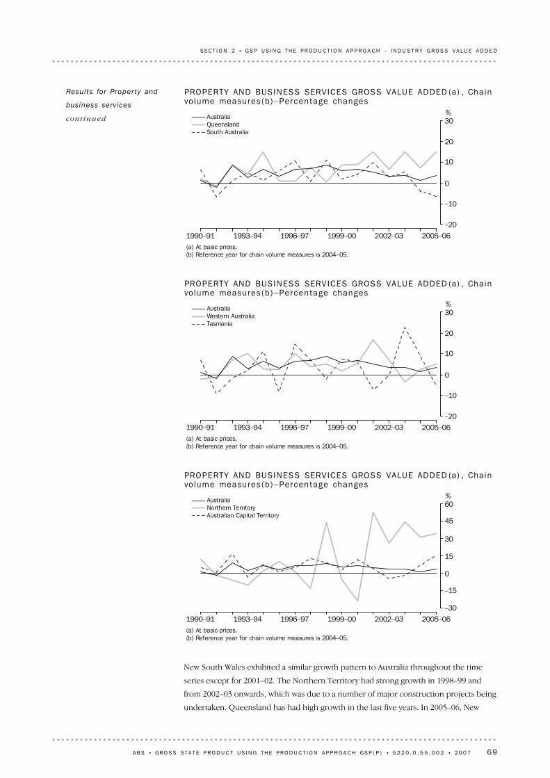
New South Wales exhibited a similar growth pattern to Australia throughout the time
series except for 2001–02. The Northern Territory had strong growth in 1998–99 and
from 2002–03 onwards, which was due to a number of major construction projects being
undertaken. Queensland has had high growth in the last five years. In 2005–06, New
(a) At basic prices.(b) Reference year for chain volume measures is 2004–05.
1990–91 1993–94 1996–97 1999–00 2002–03 2005–06
%
–30
–15
0
15
30
45
60AustraliaNorthern TerritoryAustralian Capital Territory
PROPERTY AND BUSINESS SERVICES GROSS VALUE ADDED (a) , Cha invo lume measures (b )–Percentage changes
(a) At basic prices.(b) Reference year for chain volume measures is 2004–05.
1990–91 1993–94 1996–97 1999–00 2002–03 2005–06
%
–20
–10
0
10
20
30AustraliaWestern AustraliaTasmania
PROPERTY AND BUSINESS SERVICES GROSS VALUE ADDED (a) , Cha invo lume measures (b )–Percentage changes
(a) At basic prices.(b) Reference year for chain volume measures is 2004–05.
1990–91 1993–94 1996–97 1999–00 2002–03 2005–06
%
–20
–10
0
10
20
30AustraliaQueenslandSouth Australia
PROPERTY AND BUSINESS SERVICES GROSS VALUE ADDED (a) , Cha invo lume measures (b )–Percentage changes
Results for Property and
business serv ices
cont inue d
A B S • GR O S S ST A T E P R O D U C T U S I N G T H E P R O D U C T I O N A P P R O A C H GS P ( P ) • 5 2 2 0 . 0 . 5 5 . 0 0 2 • 2 0 0 7 69
SE C T I O N 2 • G S P U S I N G T H E P R O D U C T I O N A P P R O A C H – I N D U S T R Y G R O S S V A L U E A D D E D

New South Wales and Victoria together accounted for 65.6% of Australian Property and
business services GVA in 2005–06. The state shares for these two large states and the
Northern Territory were fairly stable throughout the time series. During this period,
South Australia, Tasmania and the Australian Capital Territory marginally decreased their
shares, while Queensland and Western Australian shares were stable until 1999–2000 and
then gradually increased.
100.0100.0100.0100.0100.0100.0Australia2.22.22.32.42.62.6
Australian CapitalTerritory
0.80.80.80.70.80.7Northern Territory0.90.80.80.81.11.4Tasmania
10.59.99.68.99.38.8Western Australia5.05.25.25.46.56.2South Australia
15.114.514.013.213.713.0Queensland26.626.126.526.825.827.6Victoria39.040.440.841.840.139.7New South Wales
%%%%%%
2005–062004–052003–041999–001994–951989–90
PROPERTY AND BUSINESS SERVICES GROSS VALUE ADDED, Stateshares —Cur ren t pr ices
South Wales, South Australia and Tasmania all experienced negative growth of
–1.8%,–6.4% and –5.5% respectively.
Results for Property and
business serv ices
cont inue d
70 A B S • GR O S S ST A T E P R O D U C T U S I N G T H E P R O D U C T I O N A P P R O A C H GS P ( P ) • 5 2 2 0 . 0 . 5 5 . 0 0 2 • 2 0 0 7
SE C T I O N 2 • G S P U S I N G T H E P R O D U C T I O N A P P R O A C H – I N D U S T R Y G R O S S V A L U E A D D E D
The methodology for Government administration and defence uses an input indicator
approach to compile state by industry GVA estimates. Volume input indicators are
derived as the sum of hours worked for both Government administration employees and
Defence employees by state.
The state specific input indicators are derived by taking numbers of Government
administration and defence employees by state and multiplying them by the average
hours worked for Government administration and Defence employees by state. The
resultant hours worked by state for Government administration and Defence employees
are summed to form total division level hours worked by state.
The data on average hours worked in Government administration and defence by state is
from the ABS Labour Force, Australia. The number of Government administration
employees is from the ABS Wage and Salary Earners, Public Sector, Australia
(cat. no. 6248.0.55.001). The state ratio of defence force employees (from the
Department of Defence annual report) is used to allocate the total number of Defence
employees to state.
The state input volume indicators are used to derive volume measures of GVA for
Government administration and defence. The state volume GVAs are benchmarked to
the annual national industry volume GVA.
Summary of GSP(P)
sources and methods
The Government administration and defence industry includes central, state and local
government units mainly engaged in government administration and regulatory
activities, as well as judicial authorities and commissions, representatives of overseas
governments, and the Army, Navy and Air defence forces and civilian units mainly
engaged in defence administration.
ANZSIC Division M, Government administration and defence, consists of two
sub-divisions:
! Government administration (sub-division 81)
! Defence (sub-division 82).
GO V E R N M E N T
AD M I N I S T R A T I O N AN D
DE F E N C E
Definit ion and scope
A B S • GR O S S ST A T E P R O D U C T U S I N G T H E P R O D U C T I O N A P P R O A C H GS P ( P ) • 5 2 2 0 . 0 . 5 5 . 0 0 2 • 2 0 0 7 71
SE C T I O N 2 • G S P U S I N G T H E P R O D U C T I O N A P P R O A C H – I N D U S T R Y G R O S S V A L U E A D D E D
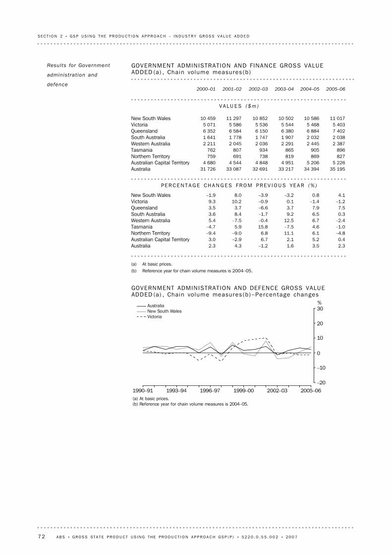
(a) At basic prices.(b) Reference year for chain volume measures is 2004–05.
1990–91 1993–94 1996–97 1999–00 2002–03 2005–06
%
–20
–10
0
10
20
30AustraliaNew South WalesVictoria
GOVERNMENT ADMINISTRAT ION AND DEFENCE GROSS VALUEADDED (a) , Cha in vo lume measures (b )–Percentage changes
(a) At basic prices.(b) Reference year for chain volume measures is 2004–05.
2.33.51.6–1.24.32.3Australia0.45.22.16.7–2.93.0Australian Capital Territory
–4.86.111.16.8–9.0–9.4Northern Territory–1.04.6–7.515.85.9–4.7Tasmania–2.46.712.5–0.4–7.55.4Western Australia0.36.59.2–1.78.43.6South Australia7.57.93.7–6.63.73.5Queensland
–1.2–1.40.1–0.910.29.3Victoria4.10.8–3.2–3.98.0–1.9New South Wales
PE R C E N T A G E CH A N G E S FR O M PR E V I O U S YE A R (% )
35 19534 39433 21732 69133 08731 726Australia5 2265 2064 9514 8484 5444 680Australian Capital Territory
827869819738691759Northern Territory896905865934807762Tasmania
2 3872 4452 2912 0362 0452 211Western Australia2 0382 0321 9071 7471 7781 641South Australia7 4026 8846 3806 1506 5846 352Queensland5 4035 4685 5445 5365 5865 071Victoria
11 01710 58610 50210 85211 29710 459New South Wales
VA L U E S ( $ m )
2005–062004–052003–042002–032001–022000–01
GOVERNMENT ADMINISTRAT ION AND FINANCE GROSS VALUEADDED (a) , Cha in vo lume measures (b )
Results for Government
administrat ion and
defence
72 A B S • GR O S S ST A T E P R O D U C T U S I N G T H E P R O D U C T I O N A P P R O A C H GS P ( P ) • 5 2 2 0 . 0 . 5 5 . 0 0 2 • 2 0 0 7
SE C T I O N 2 • G S P U S I N G T H E P R O D U C T I O N A P P R O A C H – I N D U S T R Y G R O S S V A L U E A D D E D

In 2005–06, New South Wales, Queensland, South Australia and the Australian Capital
Territory all had positive growth, with highest growth being recorded by Queensland at
7.5%.
(a) At basic prices.(b) Reference year for chain volume measures is 2004–05.
1990–91 1993–94 1996–97 1999–00 2002–03 2005–06
%
–20
–10
0
10
20
30AustraliaNorthern TerritoryAustralian Capital Territory
GOVERNMENT ADMINISTRAT ION AND DEFENCE GROSS VALUEADDED (a) , Cha in vo lume measures (b )–Percentage changes
(a) At basic prices.(b) Reference year for chain volume measures is 2004–05.
1990–91 1993–94 1996–97 1999–00 2002–03 2005–06
%
–20
–10
0
10
20
30AustraliaWestern AustraliaTasmania
GOVERNMENT ADMINISTRAT ION AND DEFENCE GROSS VALUEADDED (a) , Cha in vo lume measures (b )–Percentage changes
(a) At basic prices.(b) Reference year for chain volume measures is 2004–05.
1990–91 1993–94 1996–97 1999–00 2002–03 2005–06
%
–20
–10
0
10
20
30AustraliaQueenslandSouth Australia
GOVERNMENT ADMINISTRAT ION AND DEFENCE GROSS VALUEADDED (a) , Cha in vo lume measures (b )–Percentage changes
Results for Government
administrat ion and
defence cont inu ed
A B S • GR O S S ST A T E P R O D U C T U S I N G T H E P R O D U C T I O N A P P R O A C H GS P ( P ) • 5 2 2 0 . 0 . 5 5 . 0 0 2 • 2 0 0 7 73
SE C T I O N 2 • G S P U S I N G T H E P R O D U C T I O N A P P R O A C H – I N D U S T R Y G R O S S V A L U E A D D E D
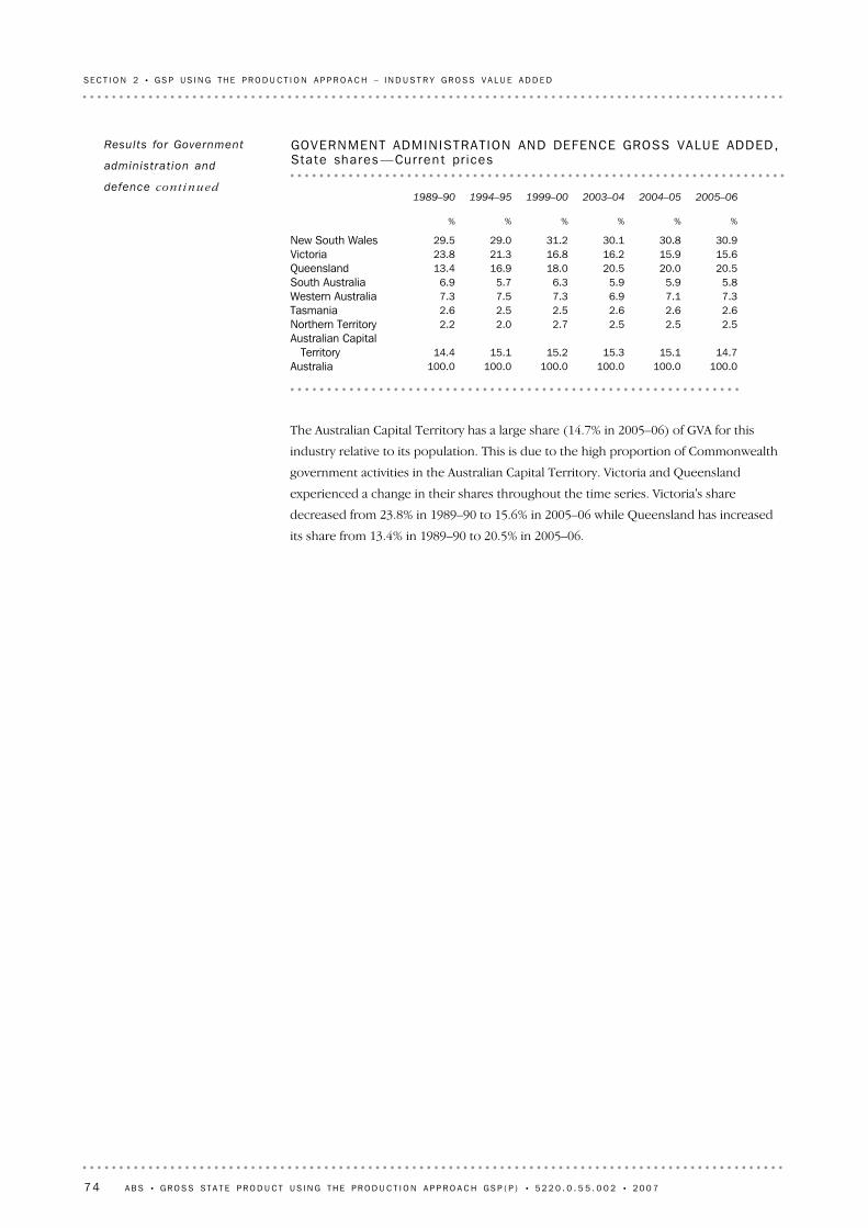
The Australian Capital Territory has a large share (14.7% in 2005–06) of GVA for this
industry relative to its population. This is due to the high proportion of Commonwealth
government activities in the Australian Capital Territory. Victoria and Queensland
experienced a change in their shares throughout the time series. Victoria's share
decreased from 23.8% in 1989–90 to 15.6% in 2005–06 while Queensland has increased
its share from 13.4% in 1989–90 to 20.5% in 2005–06.
100.0100.0100.0100.0100.0100.0Australia14.715.115.315.215.114.4
Australian CapitalTerritory
2.52.52.52.72.02.2Northern Territory2.62.62.62.52.52.6Tasmania7.37.16.97.37.57.3Western Australia5.85.95.96.35.76.9South Australia
20.520.020.518.016.913.4Queensland15.615.916.216.821.323.8Victoria30.930.830.131.229.029.5New South Wales
%%%%%%
2005–062004–052003–041999–001994–951989–90
GOVERNMENT ADMINISTRAT ION AND DEFENCE GROSS VALUE ADDED,State shares —Curren t pr ices
Results for Government
administrat ion and
defence cont inu ed
74 A B S • GR O S S ST A T E P R O D U C T U S I N G T H E P R O D U C T I O N A P P R O A C H GS P ( P ) • 5 2 2 0 . 0 . 5 5 . 0 0 2 • 2 0 0 7
SE C T I O N 2 • G S P U S I N G T H E P R O D U C T I O N A P P R O A C H – I N D U S T R Y G R O S S V A L U E A D D E D

The methodology for Education uses an output indicator approach to compile state by
industry GVA estimates. The quantity revaluation method is used to derive state specific
education output volumes for all but the latest year when price deflation is used.
Education output indicators by state are derived for each level of Education weighted
together by the cost of providing those services.
The quantity revalued output indicator uses data on the number of students in
preschools, primary and secondary schools obtained from ABS Schools, Australia
(cat. no. 4221.0), university data from the Department of Education, Science and
Training (DEST) annual report and Vocational Education & Training data from the
National Centre for Vocational Education Research (NCVER) annual statistics.
In the latest year, the current price expenditure is price deflated using an education
specific price index in the latest year. The public sector current price data are sourced
from the ABS Government Finance Statistics, Education, Australia (cat. no.
5518.0.55.001) and private sector current price data are sourced from DEST.
These state output indicators are used to derive volume measures of GVA for Education.
The state volume GVAs are then benchmarked to the annual national industry volume
GVA.
Summary of GSP(P)
sources and methods
The Education industry includes all units mainly engaged in providing education.
ANZSIC Division N, Education, consists of one sub-division:
! Education (sub-division 84).
Sub-division 84 consists of the following groups:
! Group 841 – Preschool education
! Group 842 – School education
! Group 843 – Post school education
! Group 844 – Other education.
ED U C A T I O N
Definit ion and scope
A B S • GR O S S ST A T E P R O D U C T U S I N G T H E P R O D U C T I O N A P P R O A C H GS P ( P ) • 5 2 2 0 . 0 . 5 5 . 0 0 2 • 2 0 0 7 75
SE C T I O N 2 • G S P U S I N G T H E P R O D U C T I O N A P P R O A C H – I N D U S T R Y G R O S S V A L U E A D D E D

(a) At basic prices.(b) Reference year for chain volume measures is 2004–05.
1990–91 1993–94 1996–97 1999–00 2002–03 2005–06
%
–20
–10
0
10
20
30AustraliaNew South WalesVictoria
EDUCAT ION GROSS VALUE ADDED (a) , Cha in vo lumemeasures (b )–Percentage changes
— nil or rounded to zero (including null cells)(a) At basic prices.(b) Reference year for chain volume measures is 2004–05.
1.81.41.31.61.81.7Australia–1.22.12.34.4–0.10.9Australian Capital Territory2.02.2—–1.82.8–1.4Northern Territory2.11.83.11.30.91.0Tasmania
–1.01.41.4–2.41.91.3Western Australia3.53.10.11.53.20.7South Australia3.7–0.35.01.72.94.0Queensland3.11.01.21.71.41.8Victoria0.12.0–0.42.41.20.9New South Wales
PE R C E N T A G E CH A N G E S FR O M PR E V I O U S YE A R (% )
38 55637 89137 38236 89836 31535 690Australia1 0611 0741 0521 029986987Australian Capital Territory
455446437437445433Northern Territory868850836811801794Tasmania
3 2793 3113 2643 2193 2993 239Western Australia2 8582 7612 6772 6762 6352 554South Australia7 4167 1507 1706 8306 7166 526Queensland
10 2569 9499 8499 7339 5669 433Victoria12 36412 35012 10312 15711 87211 730New South Wales
VA L U E S ( $ m )
2005–062004–052003–042002–032001–022000–01
EDUCAT ION GROSS VALUE ADDED (a) , Cha in vo lume measures (b )Results for Educat ion
76 A B S • GR O S S ST A T E P R O D U C T U S I N G T H E P R O D U C T I O N A P P R O A C H GS P ( P ) • 5 2 2 0 . 0 . 5 5 . 0 0 2 • 2 0 0 7
SE C T I O N 2 • G S P U S I N G T H E P R O D U C T I O N A P P R O A C H – I N D U S T R Y G R O S S V A L U E A D D E D

(a) At basic prices.(b) Reference year for chain volume measures is 2004–05.
1990–91 1993–94 1996–97 1999–00 2002–03 2005–06
%
–20
–10
0
10
20
30AustraliaNorthern TerritoryAustralian Capital Territory
EDUCAT ION GROSS VALUE ADDED (a) , Cha in vo lumemeasures (b )–Percentage changes
(a) At basic prices.(b) Reference year for chain volume measures is 2004–05.
1990–91 1993–94 1996–97 1999–00 2002–03 2005–06
%
–20
–10
0
10
20
30AustraliaWestern AustraliaTasmania
EDUCAT ION GROSS VALUE ADDED (a) , Cha in vo lumemeasures (b )–Percentage changes
(a) At basic prices.(b) Reference year for chain volume measures is 2004–05.
1990–91 1993–94 1996–97 1999–00 2002–03 2005–06
%
–20
–10
0
10
20
30AustraliaQueenslandSouth Australia
EDUCAT ION GROSS VALUE ADDED (a) , Cha in vo lumemeasures (b )–Percentage changes
Results for Educat ion
cont inue d
A B S • GR O S S ST A T E P R O D U C T U S I N G T H E P R O D U C T I O N A P P R O A C H GS P ( P ) • 5 2 2 0 . 0 . 5 5 . 0 0 2 • 2 0 0 7 77
SE C T I O N 2 • G S P U S I N G T H E P R O D U C T I O N A P P R O A C H – I N D U S T R Y G R O S S V A L U E A D D E D

New South Wales, Victoria and Queensland together accounted for over three quarters
of Australian Education GVA in 2005–06. New South Wales and South Australia have lost
a marginal amount of share throughout the time series, whilst Queensland has gradually
increased its share from 15.0% in 1989–90 to 18.9% in 2005–06. All other states
maintained their shares throughout the time series.
100.0100.0100.0100.0100.0100.0Australia2.72.82.92.82.72.9
Australian CapitalTerritory
1.31.21.11.21.11.1Northern Territory2.22.22.22.12.32.5Tasmania8.68.78.78.58.98.8Western Australia7.47.37.38.08.18.9South Australia
18.918.918.417.816.915.0Queensland26.526.326.625.726.527.0Victoria32.432.632.733.933.533.8New South Wales
%%%%%%
2005–062004–052003–041999–001994–951989–90
EDUCAT ION GROSS VALUE ADDED, State shares —Curren t pr icesResults for Educat ion
cont inue d
78 A B S • GR O S S ST A T E P R O D U C T U S I N G T H E P R O D U C T I O N A P P R O A C H GS P ( P ) • 5 2 2 0 . 0 . 5 5 . 0 0 2 • 2 0 0 7
SE C T I O N 2 • G S P U S I N G T H E P R O D U C T I O N A P P R O A C H – I N D U S T R Y G R O S S V A L U E A D D E D

The methodology for Health and community services uses an output indicator approach
to compile state by industry GVA estimates. Output volumes are derived using both
quantity revaluation and price deflation methods.
The current price output estimates include nine components – public hospitals, private
hospitals, public psychiatric hospitals, private psychiatric hospitals, nursing homes,
public health insurance, private health insurance, veterinary services and childcare.
Output volumes are derived using quantity revaluation of the state output for Health and
community services for the first seven components listed above and price deflation for
the last two components.
As latest year output data are not available for all components, only the four available
components are used to extrapolate the total state current price output. These four
components are nursing homes, veterinary services, private health insurance and public
health insurance.
Public hospitals, private hospitals and public psychiatric hospitals data are sourced from
the Australian Institute of Health and Welfare. Private psychiatric hospitals data are
sourced from ABS Private Hospitals, Australia (cat. no. 4390.0). Public health insurance
data are sourced from Medicare. Private health insurance data are sourced from the
Private Health Insurance Administration Council. Nursing homes data are sourced from
the Department of Health and Ageing. Veterinary services data are sourced from ABS
Retail Trade, Australia and childcare data are sourced from the Department of Family
and Community Services.
The state output indicators are used to derive volume measures of GVA for Health and
community services. The state volume GVAs are benchmarked to the annual national
industry volume GVA.
Summary of GSP(P)
sources and methods
The Health and community services industry includes all units mainly engaged in
providing health and community services.
ANZSIC Division O, Health and community services, consists of two sub-divisions:
! Health services (sub-division 86)
! Community services (sub-division 87).
HE A L T H AN D CO M M U N I T Y
SE R V I C E S
Definit ion and scope
A B S • GR O S S ST A T E P R O D U C T U S I N G T H E P R O D U C T I O N A P P R O A C H GS P ( P ) • 5 2 2 0 . 0 . 5 5 . 0 0 2 • 2 0 0 7 79
SE C T I O N 2 • G S P U S I N G T H E P R O D U C T I O N A P P R O A C H – I N D U S T R Y G R O S S V A L U E A D D E D

(a) At basic prices.(b) Reference year for chain volume measures is 2004–05.
1990–91 1993–94 1996–97 1999–00 2002–03 2005–06
%
–20
–10
0
10
20
30AustraliaNew South WalesVictoria
HEALTH AND COMMUNITY SERVICES GROSS VALUE ADDED (a) , Cha invo lume measures (b )–Percentage changes
— nil or rounded to zero (including null cells)(a) At basic prices.(b) Reference year for chain volume measures is 2004–05.
4.24.83.54.35.44.7Australia4.34.26.25.84.44.8Australian Capital Territory5.95.14.08.67.33.4Northern Territory3.12.82.3—9.32.2Tasmania4.24.72.15.53.55.5Western Australia4.34.93.24.04.46.3South Australia5.85.74.53.35.95.7Queensland4.64.63.55.95.44.3Victoria3.24.83.43.55.84.0New South Wales
PE R C E N T A G E CH A N G E S FR O M PR E V I O U S YE A R (% )
55 45553 19750 74549 03647 00844 582Australia1 1221 0761 032972919880Australian Capital Territory
655619588566521486Northern Territory1 3881 3461 3091 2791 2791 170Tasmania5 6805 4525 2095 1034 8364 674Western Australia4 4494 2664 0663 9393 7873 627South Australia9 7169 1838 6888 3178 0507 603Queensland
14 24113 61813 02312 58311 87911 269Victoria18 20417 63816 82916 27315 73014 868New South Wales
VA L U E S ( $ m )
2005–062004–052003–042002–032001–022000–01
HEALTH AND COMMUNITY SERVICES GROSS VALUE ADDED (a) , Cha invo lume measures (b )
Results for Health and
community serv ices
80 A B S • GR O S S ST A T E P R O D U C T U S I N G T H E P R O D U C T I O N A P P R O A C H GS P ( P ) • 5 2 2 0 . 0 . 5 5 . 0 0 2 • 2 0 0 7
SE C T I O N 2 • G S P U S I N G T H E P R O D U C T I O N A P P R O A C H – I N D U S T R Y G R O S S V A L U E A D D E D

Throughout the time series all states experienced positive growth in the Health and
community services industry. New South Wales, Victoria, South Australia and
Queensland exhibited a similar growth pattern to Australia throughout the time series.
Western Australia and Tasmania exhibited a growth similar to Australia up to 1996–97
(a) At basic prices.(b) Reference year for chain volume measures is 2004–05.
1990–91 1993–94 1996–97 1999–00 2002–03 2005–06
%
–20
–10
0
10
20
30AustraliaNorthern TerritoryAustralian Capital Territory
HEALTH AND COMMUNITY SERVICES GROSS VALUE ADDED (a) , Cha invo lume measures (b )–Percentage changes
(a) At basic prices.(b) Reference year for chain volume measures is 2004–05.
1990–91 1993–94 1996–97 1999–00 2002–03 2005–06
%
–20
–10
0
10
20
30AustraliaWestern AustraliaTasmania
HEALTH AND COMMUNITY SERVICES GROSS VALUE ADDED (a) , Cha invo lume measures (b )–Percentage changes
(a) At basic prices.(b) Reference year for chain volume measures is 2004–05.
1990–91 1993–94 1996–97 1999–00 2002–03 2005–06
%
–20
–10
0
10
20
30AustraliaQueenslandSouth Australia
HEALTH AND COMMUNITY SERVICES GROSS VALUE ADDED (a) , Cha invo lume measures (b )–Percentage changes
Results for Health and
community serv ices
cont inue d
A B S • GR O S S ST A T E P R O D U C T U S I N G T H E P R O D U C T I O N A P P R O A C H GS P ( P ) • 5 2 2 0 . 0 . 5 5 . 0 0 2 • 2 0 0 7 81
SE C T I O N 2 • G S P U S I N G T H E P R O D U C T I O N A P P R O A C H – I N D U S T R Y G R O S S V A L U E A D D E D

The Australian Health and community services industry is dominated by New South
Wales, Victoria and Queensland, which together accounted for 75.8% of Australian
Health and community services GVA in 2005–06. There has not been any significant
change in state shares for this industry over the time series, except for Queensland
which has had growth from 14.1% in 1989-90 to 18.3% in 2005-06.
100.0100.0100.0100.0100.0100.0Australia1.92.02.02.01.71.6
Australian CapitalTerritory
1.21.21.11.21.01.0Northern Territory2.62.52.52.62.62.8Tasmania
10.410.210.610.29.79.4Western Australia8.08.08.18.59.710.0South Australia
18.317.316.916.315.914.1Queensland25.025.625.325.227.226.9Victoria32.533.233.534.232.234.3New South Wales
%%%%%%
2005–062004–052003–041999–001994–951989–90
HEALTH AND COMMUNITY SERVICES GROSS VALUE ADDED, Stateshares —Cur ren t pr ices
and the Northern Territory and the Australian Capital Territory up to 1999–2000 after
which differences emerged. In 2005–06, Queensland and the Northern Territory had
strong growth of 5.8% and 5.9% respectively.
Results for Health and
community serv ices
cont inue d
82 A B S • GR O S S ST A T E P R O D U C T U S I N G T H E P R O D U C T I O N A P P R O A C H GS P ( P ) • 5 2 2 0 . 0 . 5 5 . 0 0 2 • 2 0 0 7
SE C T I O N 2 • G S P U S I N G T H E P R O D U C T I O N A P P R O A C H – I N D U S T R Y G R O S S V A L U E A D D E D

The methodology for Cultural and recreational services uses an output indicator
approach to compile state by industry GVA estimates. Output volumes are derived using
price deflation of the state output indicators for Cultural and recreational services. The
output volumes then form the basis upon which volume measures of value added are
derived.
The private sector output indicators used are current price income from the sales of
goods and services by state for the Cultural and recreational services industry collected in
QBIS from 2001–02. Prior to QBIS the annual national industry current price GVA is split
using state weights based on QBIS. Private sector state deflators for Cultural and
recreational services are derived using components of the CPI by capital city and HFCE
implicit price deflators.
The public sector output indicators are annual current price estimates of government
expenditure on Cultural and recreational services by state, sourced from the ABS
Government Finance Statistics, Australia (GFS) (cat. no. 5512.0). These estimates are
deflated using the implicit price deflators for Government final consumption
expenditure (GFCE) (excluding Defence) split into Commonwealth and State and Local
Government by state.
The state volume GVAs are then benchmarked to the annual national industry volume
GVA.
Summary of GSP(P)
sources and methods
The Cultural and recreational services industry includes all units mainly engaged in
providing cultural and recreational facilities and services.
ANZSIC Division P, Cultural and recreational services, consists of three sub-divisions:
! Motion pictures, radio and television services (sub-division 91)
! Library, museums and the arts (sub-division 92)
! Sport and recreation (sub-division 93).
CU L T U R A L AN D
RE C R E A T I O N A L SE R V I C E S
Definit ion and scope
A B S • GR O S S ST A T E P R O D U C T U S I N G T H E P R O D U C T I O N A P P R O A C H GS P ( P ) • 5 2 2 0 . 0 . 5 5 . 0 0 2 • 2 0 0 7 83
SE C T I O N 2 • G S P U S I N G T H E P R O D U C T I O N A P P R O A C H – I N D U S T R Y G R O S S V A L U E A D D E D

(a) At basic prices.(b) Reference year for chain volume measures is 2004–05.
1990–91 1993–94 1996–97 1999–00 2002–03 2005–06
%
–20
–10
0
10
20
30AustraliaNew South WalesVictoria
CULTURAL AND RECREAT IONAL SERVICES GROSS VALUE ADDED (a) ,Cha in vo lume measures (b )–Percentage changes
(a) At basic prices.(b) Reference year for chain volume measures is 2004–05.
2.85.85.83.70.57.0Australia5.77.27.57.00.812.3Australian Capital Territory
–2.08.313.019.810.112.3Northern Territory0.56.24.95.33.88.2Tasmania
–0.45.85.73.6–1.62.6Western Australia0.84.17.30.50.84.1South Australia1.49.210.58.44.54.6Queensland3.84.52.91.43.38.9Victoria3.75.65.53.2–3.07.1New South Wales
PE R C E N T A G E CH A N G E S FR O M PR E V I O U S YE A R (% )
13 50613 13212 40911 73311 30911 252Australia552522487453423420Australian Capital Territory193197182161134122Northern Territory210209197188178172Tasmania
1 0451 049991938905919Western Australia850843810755751745South Australia
1 8291 8041 6521 4951 3791 319Queensland3 6643 5303 3773 2823 2363 134Victoria5 1634 9784 7154 4714 3334 465New South Wales
VA L U E S ( $ m )
2005–062004–052003–042002–032001–022000–01
CULTURAL AND RECREAT IONAL SERVICES GROSS VALUE ADDED (a) ,Cha in vo lume measures (b )
Results for Cultural and
recreat ional serv ices
84 A B S • GR O S S ST A T E P R O D U C T U S I N G T H E P R O D U C T I O N A P P R O A C H GS P ( P ) • 5 2 2 0 . 0 . 5 5 . 0 0 2 • 2 0 0 7
SE C T I O N 2 • G S P U S I N G T H E P R O D U C T I O N A P P R O A C H – I N D U S T R Y G R O S S V A L U E A D D E D
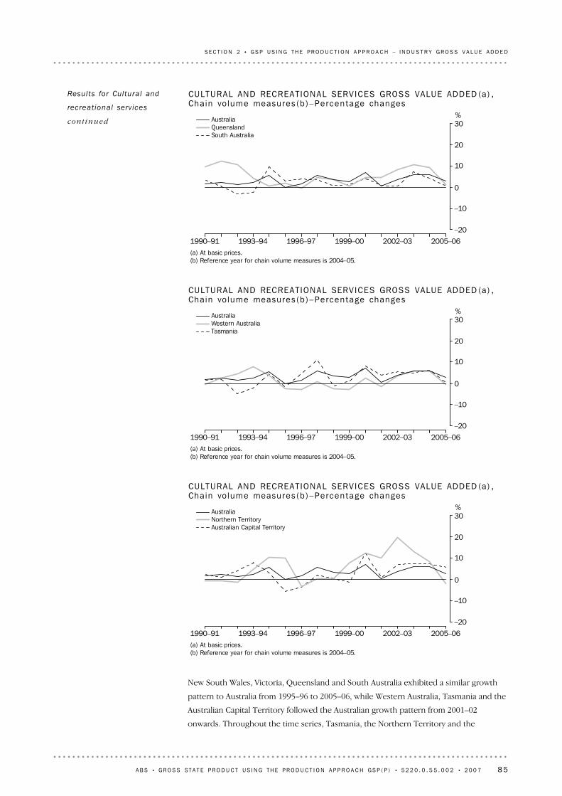
New South Wales, Victoria, Queensland and South Australia exhibited a similar growth
pattern to Australia from 1995–96 to 2005–06, while Western Australia, Tasmania and the
Australian Capital Territory followed the Australian growth pattern from 2001–02
onwards. Throughout the time series, Tasmania, the Northern Territory and the
(a) At basic prices.(b) Reference year for chain volume measures is 2004–05.
1990–91 1993–94 1996–97 1999–00 2002–03 2005–06
%
–20
–10
0
10
20
30AustraliaNorthern TerritoryAustralian Capital Territory
CULTURAL AND RECREAT IONAL SERVICES GROSS VALUE ADDED (a) ,Cha in vo lume measures (b )–Percentage changes
(a) At basic prices.(b) Reference year for chain volume measures is 2004–05.
1990–91 1993–94 1996–97 1999–00 2002–03 2005–06
%
–20
–10
0
10
20
30AustraliaWestern AustraliaTasmania
CULTURAL AND RECREAT IONAL SERVICES GROSS VALUE ADDED (a) ,Cha in vo lume measures (b )–Percentage changes
(a) At basic prices.(b) Reference year for chain volume measures is 2004–05.
1990–91 1993–94 1996–97 1999–00 2002–03 2005–06
%
–20
–10
0
10
20
30AustraliaQueenslandSouth Australia
CULTURAL AND RECREAT IONAL SERVICES GROSS VALUE ADDED (a) ,Cha in vo lume measures (b )–Percentage changes
Results for Cultural and
recreat ional serv ices
cont inue d
A B S • GR O S S ST A T E P R O D U C T U S I N G T H E P R O D U C T I O N A P P R O A C H GS P ( P ) • 5 2 2 0 . 0 . 5 5 . 0 0 2 • 2 0 0 7 85
SE C T I O N 2 • G S P U S I N G T H E P R O D U C T I O N A P P R O A C H – I N D U S T R Y G R O S S V A L U E A D D E D

New South Wales, Victoria and Queensland accounted for around 78% of Australian
Cultural and recreational services GVA in 2005–06. New South Wales lost the most share
during the time series, from 44.9% in 1989–90 down to 37.1% in 2005–06. During the
same period, Victoria, Queensland and Western Australia increased their shares, with
Victoria increasing the most, from 21.4% in 1989–90 to 27.2% in 2005–06. Tasmania and
the Northern Territory had stable shares throughout the time series.
100.0100.0100.0100.0100.0100.0Australia3.94.04.14.44.64.6
Australian CapitalTerritory
1.41.51.41.71.71.2Northern Territory1.81.61.61.51.71.9Tasmania8.58.08.37.97.77.1Western Australia6.36.46.67.37.57.7South Australia
13.813.713.712.913.811.2Queensland27.226.926.926.325.921.4Victoria37.137.937.438.037.144.9New South Wales
%%%%%%
2005–062004–052003–041999–001994–951989–90
CULTURAL AND RECREAT IONAL SERVICES GROSS VALUE ADDED, Stateshares —Cur ren t pr ices
Australian Capital Territory had variable growth patterns while all other states exhibited
more consistent growth patterns. All states experienced moderate to high growth during
2000–01, in part due to the impacts of the Sydney Olympics. In 2005–06, all states were
coming off the growth peaks experienced in the last three years with Western Australia
and the Northern Territory exhibiting negative growth rates.
Results for Cultural and
recreat ional serv ices
cont inue d
86 A B S • GR O S S ST A T E P R O D U C T U S I N G T H E P R O D U C T I O N A P P R O A C H GS P ( P ) • 5 2 2 0 . 0 . 5 5 . 0 0 2 • 2 0 0 7
SE C T I O N 2 • G S P U S I N G T H E P R O D U C T I O N A P P R O A C H – I N D U S T R Y G R O S S V A L U E A D D E D
The methodology for Personal and other services uses an output indicator approach to
compile state by industry GVA estimates. Personal and other services are produced by
both public and private sectors, consequently, the output indicators are derived as the
sum of public and private output. An output indicator method is derived for both the
public and private sectors using the price deflation method.
Public sector current price data are sourced from the ABS GFS. A deflator is derived
using wage prices from the ABS Labour Price Index, and materials prices taken from the
PPI and Import Price Index, Australia (cat. no. 6414.0). These current price and deflator
estimates are used to construct a volume indicator for the public sector.
Private sector current price estimates by state are sourced from QBIS. Prior to QBIS the
movements in the national current price private sector turnover are used to backcast the
state QBIS estimates. Private sector deflators are constructed using various components
of the ABS CPI by capital city, and HFCE implicit price deflators by state. The output
volume estimates are then used to derive volume estimates for the private sector.
The state output indicators are used to derive volume measures of GVA for Personal and
other services. The state volume GVAs are then benchmarked to the annual national
industry volume GVA.
Summary of GSP(P)
sources and methods
The Personal and other services industry includes all units mainly engaged in providing
personal services.
ANZSIC93 Division Q, Personal and other services, consists of three sub-divisions:
! Personal services (sub-division 95)
! Other services (sub-division 96)
! Private households employing staff (sub-division 97).
PE R S O N A L AN D OT H E R
SE R V I C E S
Definit ion and scope
A B S • GR O S S ST A T E P R O D U C T U S I N G T H E P R O D U C T I O N A P P R O A C H GS P ( P ) • 5 2 2 0 . 0 . 5 5 . 0 0 2 • 2 0 0 7 87
SE C T I O N 2 • G S P U S I N G T H E P R O D U C T I O N A P P R O A C H – I N D U S T R Y G R O S S V A L U E A D D E D

(a) At basic prices.(b) Reference year for chain volume measures is 2004–05.
1990–91 1993–94 1996–97 1999–00 2002–03 2005–06
%
–20
–10
0
10
20
30AustraliaNew South WalesVictoria
PERSONAL AND OTHER SERVICES GROSS VALUE ADDED (a) , Cha invo lume measures (b )–Percentage changes
(a) At basic prices.(b) Reference year for chain volume measures is 2004–05.
5.61.31.32.14.06.0Australia3.4–10.8–0.23.314.56.0Australian Capital Territory
18.86.15.3–11.9–8.74.5Northern Territory–0.33.112.52.94.94.1Tasmania20.85.90.12.3–1.33.2Western Australia
1.5–8.64.72.42.16.7South Australia7.13.4–2.0–3.511.210.0Queensland
13.87.4–0.3–1.32.72.6Victoria–5.0–2.33.27.82.57.0New South Wales
PE R C E N T A G E CH A N G E S FR O M PR E V I O U S YE A R (% )
17 68616 74316 52516 30715 97315 354Australia527509571572553483Australian Capital Territory280235222211239262Northern Territory320321311276268256Tasmania
2 1851 8091 7081 7061 6681 689Western Australia1 3531 3341 4601 3951 3621 334South Australia3 4253 1993 0933 1553 2692 939Queensland4 4133 8783 6113 6233 6723 575Victoria5 1845 4585 5865 4145 0204 897New South Wales
VA L U E S ( $ m )
2005–062004–052003–042002–032001–022000–01
PERSONAL AND OTHER SERVICES GROSS VALUE ADDED (a) , Cha invo lume measures (b )
Results for Personal and
other serv ices
88 A B S • GR O S S ST A T E P R O D U C T U S I N G T H E P R O D U C T I O N A P P R O A C H GS P ( P ) • 5 2 2 0 . 0 . 5 5 . 0 0 2 • 2 0 0 7
SE C T I O N 2 • G S P U S I N G T H E P R O D U C T I O N A P P R O A C H – I N D U S T R Y G R O S S V A L U E A D D E D

In 2005–06, New South Wales and Tasmania experienced negative growth whereas
Victoria, Western Australia and the Northern Territory had strong growth of 13.8%, 20.8%
and 18.8% respectively, reflecting increases in both private and public expenditure.
(a) At basic prices.(b) Reference year for chain volume measures is 2004–05.
1990–91 1993–94 1996–97 1999–00 2002–03 2005–06
%
–20
–10
0
10
20
30AustraliaNorthern TerritoryAustralian Capital Territory
PERSONAL AND OTHER SERVICES GROSS VALUE ADDED (a) , Cha invo lume measures (b )–Percentage changes
(a) At basic prices.(b) Reference year for chain volume measures is 2004–05.
1990–91 1993–94 1996–97 1999–00 2002–03 2005–06
%
–20
–10
0
10
20
30AustraliaWestern AustraliaTasmania
PERSONAL AND OTHER SERVICES GROSS VALUE ADDED (a) , Cha invo lume measures (b )–Percentage changes
(a) At basic prices.(b) Reference year for chain volume measures is 2004–05.
1990–91 1993–94 1996–97 1999–00 2002–03 2005–06
%
–20
–10
0
10
20
30AustraliaQueenslandSouth Australia
PERSONAL AND OTHER SERVICES GROSS VALUE ADDED (a) , Cha invo lume measures (b )–Percentage changes
Results for Personal and
other serv ices cont inu ed
A B S • GR O S S ST A T E P R O D U C T U S I N G T H E P R O D U C T I O N A P P R O A C H GS P ( P ) • 5 2 2 0 . 0 . 5 5 . 0 0 2 • 2 0 0 7 89
SE C T I O N 2 • G S P U S I N G T H E P R O D U C T I O N A P P R O A C H – I N D U S T R Y G R O S S V A L U E A D D E D

New South Wales, Victoria and Queensland accounted for almost 75% of total Australian
Personal and other services GVA in 2005-06. New South Wales lost share steadily
throughout the time series, moving from 39.2% in 1989–90 to 31.9% in 2005–06.
Queensland increased its share from 12.7% in 1989–90 to 21.1% in 2005–06. Victoria,
Tasmania, the Northern Territory and the Australian Capital Territory had quite stable
shares throughout the time series.
100.0100.0100.0100.0100.0100.0Australia3.03.03.13.03.13.1
Australian CapitalTerritory
1.41.41.41.41.31.1Northern Territory2.11.92.01.92.02.3Tasmania
10.910.810.710.310.99.3Western Australia7.88.08.28.29.89.8South Australia
21.119.119.218.516.112.7Queensland21.823.222.622.522.222.5Victoria31.932.632.834.134.739.2New South Wales
%%%%%%
2005–062004–052003–041999–001994–951989–90
PERSONAL AND OTHER SERVICES GROSS VALUE ADDED, Stateshares —Cur ren t pr ices
Results for Personal and
other serv ices cont inu ed
90 A B S • GR O S S ST A T E P R O D U C T U S I N G T H E P R O D U C T I O N A P P R O A C H GS P ( P ) • 5 2 2 0 . 0 . 5 5 . 0 0 2 • 2 0 0 7
SE C T I O N 2 • G S P U S I N G T H E P R O D U C T I O N A P P R O A C H – I N D U S T R Y G R O S S V A L U E A D D E D

The methodology for Ownership of dwellings uses an output indicator approach to
compile state by industry GVA estimates. Output volumes are derived using the HFCE
volumes of rent. The state volume GVAs are benchmarked to the annual national
industry volume GVA.
Summary of GSP(P)
sources and methods
Ownership of dwellings consists of landlords and owner-occupiers of dwellings.
Owner-occupiers are regarded as operating a business that generates a gross operating
surplus. The imputation of a rent to owner-occupied dwellings enables the services
provided by dwellings to their owner-occupiers to be treated consistently with the
marketed services provided by rented dwellings to their tenants. Owner-occupiers are
regarded as receiving rents (from themselves as consumers), paying expenses, and
making a net contribution to the value of production which accrues to them as owners.
OW N E R S H I P OF
DW E L L I N G S
Definit ion and scope
A B S • GR O S S ST A T E P R O D U C T U S I N G T H E P R O D U C T I O N A P P R O A C H GS P ( P ) • 5 2 2 0 . 0 . 5 5 . 0 0 2 • 2 0 0 7 91
SE C T I O N 2 • G S P U S I N G T H E P R O D U C T I O N A P P R O A C H – I N D U S T R Y G R O S S V A L U E A D D E D

(a) At basic prices.(b) Reference year for chain volume measures is 2004–05.
1990–91 1993–94 1996–97 1999–00 2002–03 2005–06
%
0
2
4
6
8AustraliaNew South WalesVictoria
OWNERSHIP OF DWELL INGS GROSS VALUE ADDED (a) , Cha in vo lumemeasures (b )–Percentage changes
(a) At basic prices.(b) Reference year for chain volume measures is 2004–05.
3.94.33.94.03.83.8Australia3.84.13.73.83.73.8Australian Capital Territory4.04.43.83.73.73.8Northern Territory3.84.23.93.93.63.5Tasmania4.14.44.04.03.93.8Western Australia3.74.23.73.83.73.6South Australia4.14.54.24.34.14.0Queensland3.94.33.94.03.83.8Victoria3.84.23.73.93.83.8New South Wales
PE R C E N T A G E CH A N G E S FR O M PR E V I O U S YE A R (% )
73 67370 92768 00265 47362 97860 647Australia1 6611 6001 5371 4831 4291 377Australian Capital Territory
980943903871840810Northern Territory1 1671 1241 0791 0391 000965Tasmania6 6356 3766 1065 8735 6465 436Western Australia5 0184 8394 6464 4804 3164 163South Australia
12 99112 48411 94511 46610 99310 557Queensland17 68617 02816 32415 71615 11714 559Victoria27 53526 53125 45924 53923 62722 766New South Wales
VA L U E S ( $ m )
2005–062004–052003–042002–032001–022000–01
OWNERSHIP OF DWELL INGS GROSS VALUE ADDED (a) , Cha in vo lumemeasures (b )
Results for Ownership of
dwell ings
92 A B S • GR O S S ST A T E P R O D U C T U S I N G T H E P R O D U C T I O N A P P R O A C H GS P ( P ) • 5 2 2 0 . 0 . 5 5 . 0 0 2 • 2 0 0 7
SE C T I O N 2 • G S P U S I N G T H E P R O D U C T I O N A P P R O A C H – I N D U S T R Y G R O S S V A L U E A D D E D

All states exhibited a positive growth pattern similar to Australia throughout the time
series. The rise in growth in 1996–97 is related to the fall in interest rates from around
10% in 1995–96 to around 7% in 1996–97. Since 2000–01, all states have exhibited growth
rates around 4%.
(a) At basic prices(b) Reference year for chain volume measures is 2004–05.
1990–91 1993–94 1996–97 1999–00 2002–03 2005–06
%
0
2
4
6
8AustraliaNorthern TerritoryAustralian Capital Territory
OWNERSHIP OF DWELL INGS GROSS VALUE ADDED (a) , Cha in vo lumemeasures (b )–Percentage changes
(a) At basic prices.(b) Reference year for chain volume measures is 2004–05.
1990–91 1993–94 1996–97 1999–00 2002–03 2005–06
%
0
2
4
6
8AustraliaWestern AustraliaTasmania
OWNERSHIP OF DWELL INGS GROSS VALUE ADDED (a) , Cha in vo lumemeasures (b )–Percentage changes
(a) At basic prices.(b) Reference year for chain volume measures is 2004–05.
1990–91 1993–94 1996–97 1999–00 2002–03 2005–06
%
0
2
4
6
8AustraliaQueenslandSouth Australia
OWNERSHIP OF DWELL INGS GROSS VALUE ADDED (a) , Cha in vo lumemeasures (b )–Percentage changes
Results for Ownership of
dwell ings cont inued
A B S • GR O S S ST A T E P R O D U C T U S I N G T H E P R O D U C T I O N A P P R O A C H GS P ( P ) • 5 2 2 0 . 0 . 5 5 . 0 0 2 • 2 0 0 7 93
SE C T I O N 2 • G S P U S I N G T H E P R O D U C T I O N A P P R O A C H – I N D U S T R Y G R O S S V A L U E A D D E D
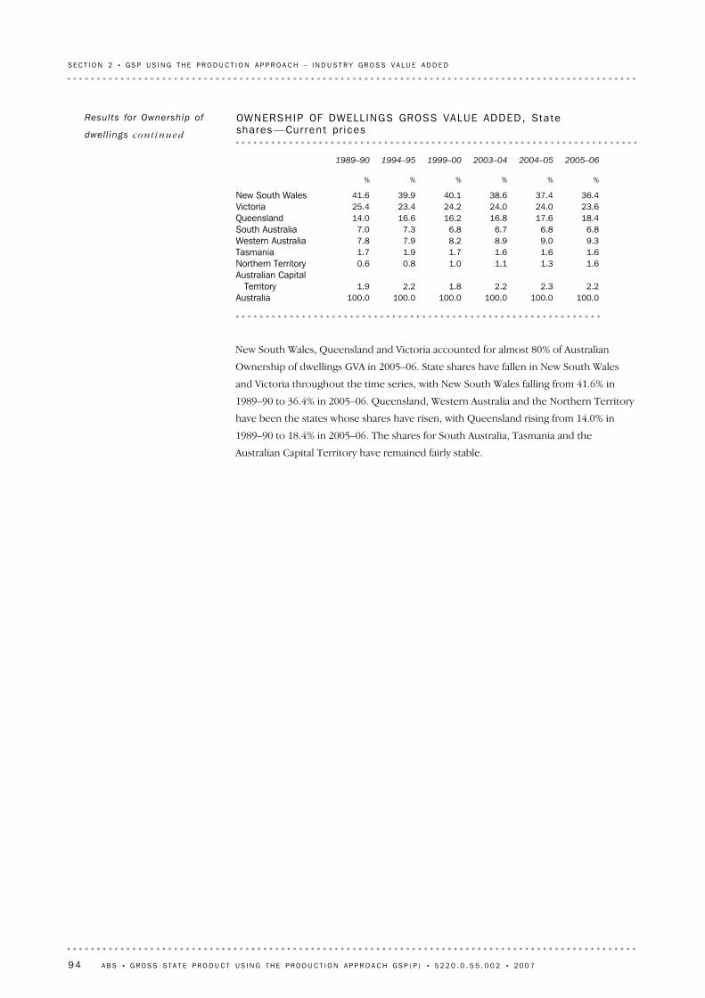
New South Wales, Queensland and Victoria accounted for almost 80% of Australian
Ownership of dwellings GVA in 2005–06. State shares have fallen in New South Wales
and Victoria throughout the time series, with New South Wales falling from 41.6% in
1989–90 to 36.4% in 2005–06. Queensland, Western Australia and the Northern Territory
have been the states whose shares have risen, with Queensland rising from 14.0% in
1989–90 to 18.4% in 2005–06. The shares for South Australia, Tasmania and the
Australian Capital Territory have remained fairly stable.
100.0100.0100.0100.0100.0100.0Australia2.22.32.21.82.21.9
Australian CapitalTerritory
1.61.31.11.00.80.6Northern Territory1.61.61.61.71.91.7Tasmania9.39.08.98.27.97.8Western Australia6.86.86.76.87.37.0South Australia
18.417.616.816.216.614.0Queensland23.624.024.024.223.425.4Victoria36.437.438.640.139.941.6New South Wales
%%%%%%
2005–062004–052003–041999–001994–951989–90
OWNERSHIP OF DWELL INGS GROSS VALUE ADDED, Stateshares —Cur ren t pr ices
Results for Ownership of
dwell ings cont inued
94 A B S • GR O S S ST A T E P R O D U C T U S I N G T H E P R O D U C T I O N A P P R O A C H GS P ( P ) • 5 2 2 0 . 0 . 5 5 . 0 0 2 • 2 0 0 7
SE C T I O N 2 • G S P U S I N G T H E P R O D U C T I O N A P P R O A C H – I N D U S T R Y G R O S S V A L U E A D D E D

Commonwealth taxes have been allocated to states using HFCE, imports or GVA
depending on the type of tax. This allocation of Commonwealth taxes is then combined
with the State taxes to produce a total Taxes on products for each state.
Volume estimates of Taxes on products are produced using quantity revaluation. The
indicators used for quantity revaluation depend on each individual tax. For example,
Sales tax is based around the taxation revenue collected and total wholesale sale
volumes. Taxes on crude oil is based on the taxation revenue collected and the quantity
of petroleum produced.
Subsidies on products are only a small proportion of Taxes less subsidies on products.
State subsidies have been combined with a state share of Commonwealth subsidies
which have been allocated to states based on Taxes less subsidies on production and
imports shares.
The output indicator (i.e. Total taxes less subsidies on production) is calculated as the
difference between total Taxes on products and total Subsidies on products for each
state. The state output indicators are used to derive volume measures of Taxes less
subsidies on products. The state volume Taxes less subsidies on products estimates are
benchmarked to the annual national industry volume Taxes less subsidies on products
estimates.
Summary of GSP(P)
sources and methods
Taxes on products are levied by both the States and the Commonwealth. Taxes on
products include taxes on the provision of goods and services (e.g. sales tax and GST),
excises, taxes on international trade, taxes on gambling, taxes on insurance, etc.
Subsidies on products are paid by governments to the producer for the production of a
particular product.
TA X E S LE S S SU B S I D I E S
ON PR O D U C T S
Definit ion and scope
A B S • GR O S S ST A T E P R O D U C T U S I N G T H E P R O D U C T I O N A P P R O A C H GS P ( P ) • 5 2 2 0 . 0 . 5 5 . 0 0 2 • 2 0 0 7 95
SE C T I O N 2 • G S P U S I N G T H E P R O D U C T I O N A P P R O A C H – I N D U S T R Y G R O S S V A L U E A D D E D
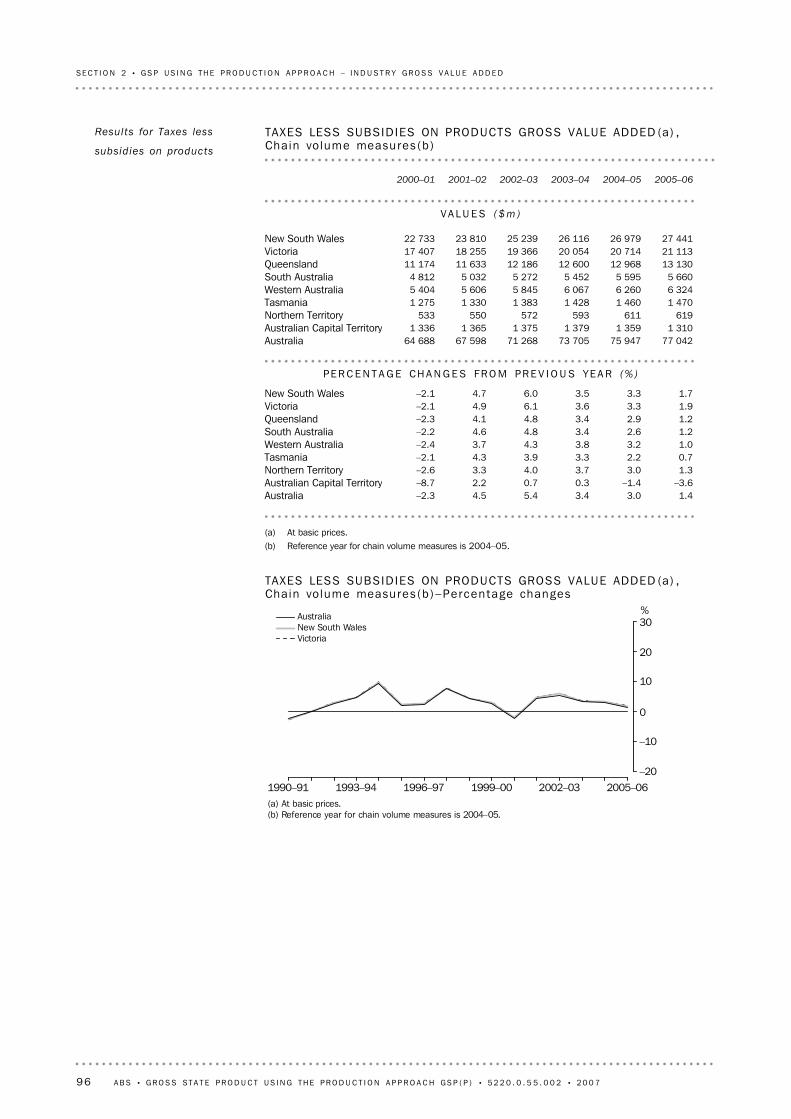
(a) At basic prices.(b) Reference year for chain volume measures is 2004–05.
1990–91 1993–94 1996–97 1999–00 2002–03 2005–06
%
–20
–10
0
10
20
30AustraliaNew South WalesVictoria
TAXES LESS SUBSID IES ON PRODUCTS GROSS VALUE ADDED (a) ,Cha in vo lume measures (b )–Percentage changes
(a) At basic prices.(b) Reference year for chain volume measures is 2004–05.
1.43.03.45.44.5–2.3Australia–3.6–1.40.30.72.2–8.7Australian Capital Territory1.33.03.74.03.3–2.6Northern Territory0.72.23.33.94.3–2.1Tasmania1.03.23.84.33.7–2.4Western Australia1.22.63.44.84.6–2.2South Australia1.22.93.44.84.1–2.3Queensland1.93.33.66.14.9–2.1Victoria1.73.33.56.04.7–2.1New South Wales
PE R C E N T A G E CH A N G E S FR O M PR E V I O U S YE A R (% )
77 04275 94773 70571 26867 59864 688Australia1 3101 3591 3791 3751 3651 336Australian Capital Territory
619611593572550533Northern Territory1 4701 4601 4281 3831 3301 275Tasmania6 3246 2606 0675 8455 6065 404Western Australia5 6605 5955 4525 2725 0324 812South Australia
13 13012 96812 60012 18611 63311 174Queensland21 11320 71420 05419 36618 25517 407Victoria27 44126 97926 11625 23923 81022 733New South Wales
VA L U E S ( $ m )
2005–062004–052003–042002–032001–022000–01
TAXES LESS SUBSID IES ON PRODUCTS GROSS VALUE ADDED (a) ,Cha in vo lume measures (b )
Results for Taxes less
subsid ies on products
96 A B S • GR O S S ST A T E P R O D U C T U S I N G T H E P R O D U C T I O N A P P R O A C H GS P ( P ) • 5 2 2 0 . 0 . 5 5 . 0 0 2 • 2 0 0 7
SE C T I O N 2 • G S P U S I N G T H E P R O D U C T I O N A P P R O A C H – I N D U S T R Y G R O S S V A L U E A D D E D

Throughout the time series, all states generally exhibited a similar growth pattern to
Australia.
(a) At basic prices.(b) Reference year for chain volume measures is 2004–05.
1990–91 1993–94 1996–97 1999–00 2002–03 2005–06
%
–20
–10
0
10
20
30AustraliaNorthern TerritoryAustralian Capital Territory
TAXES LESS SUBSID IES ON PRODUCTS GROSS VALUE ADDED (a) ,Cha in vo lume measures (b )–Percentage changes
(a) At basic prices.(b) Reference year for chain volume measures is 2004–05.
1990–91 1993–94 1996–97 1999–00 2002–03 2005–06
%
–20
–10
0
10
20
30AustraliaWestern AustraliaTasmania
TAXES LESS SUBSID IES ON PRODUCTS GROSS VALUE ADDED (a) ,Cha in vo lume measures (b )–Percentage changes
(a) At basic prices.(b) Reference year for chain volume measures is 2004–05.
1990–91 1993–94 1996–97 1999–00 2002–03 2005–06
%
–20
–10
0
10
20
30AustraliaQueenslandSouth Australia
TAXES LESS SUBSID IES ON PRODUCTS GROSS VALUE ADDED (a) ,Cha in vo lume measures (b )–Percentage changes
Results for Taxes less
subsid ies on products
cont inue d
A B S • GR O S S ST A T E P R O D U C T U S I N G T H E P R O D U C T I O N A P P R O A C H GS P ( P ) • 5 2 2 0 . 0 . 5 5 . 0 0 2 • 2 0 0 7 97
SE C T I O N 2 • G S P U S I N G T H E P R O D U C T I O N A P P R O A C H – I N D U S T R Y G R O S S V A L U E A D D E D
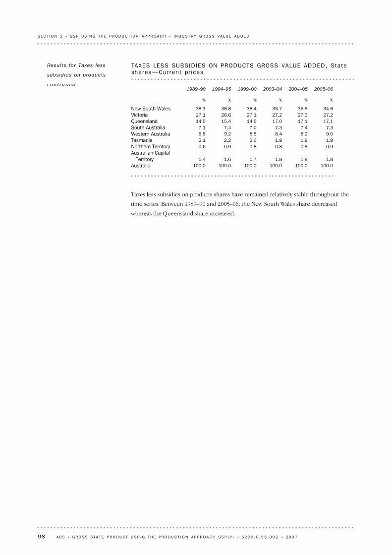
Taxes less subsidies on products shares have remained relatively stable throughout the
time series. Between 1989–90 and 2005–06, the New South Wales share decreased
whereas the Queensland share increased.
100.0100.0100.0100.0100.0100.0Australia1.81.81.81.71.61.4
Australian CapitalTerritory
0.90.80.80.80.90.6Northern Territory1.91.91.92.02.22.1Tasmania9.08.28.48.59.28.8Western Australia7.37.47.37.07.47.1South Australia
17.117.117.014.515.414.5Queensland27.227.327.227.126.627.1Victoria34.635.535.738.436.838.3New South Wales
%%%%%%
2005–062004–052003–041999–001994–951989–90
TAXES LESS SUBSID IES ON PRODUCTS GROSS VALUE ADDED, Stateshares —Cur ren t pr ices
Results for Taxes less
subsid ies on products
cont inue d
98 A B S • GR O S S ST A T E P R O D U C T U S I N G T H E P R O D U C T I O N A P P R O A C H GS P ( P ) • 5 2 2 0 . 0 . 5 5 . 0 0 2 • 2 0 0 7
SE C T I O N 2 • G S P U S I N G T H E P R O D U C T I O N A P P R O A C H – I N D U S T R Y G R O S S V A L U E A D D E D

SECT I O N 3 CO N C L U S I O N AN D FU T U R E D I R E C T I O N S . . . . . . . . . . .
There are a number of areas that require further research in order to be able to maximise
the quality of estimates. These areas include:
FU T U R E RE S E A R C H
AG E N D A
Owing to the inclusion of the GSP(P) and GVA by industry estimates, a number of
changes to the layout of 5220.0 will be made:
! Headline GSP, in both current prices and volume terms, will be based on the simple
average of available measures.
! A statistical discrepancy (relative to GSP(A)) will be included for both volume and
current price tables.
! Tables providing GVA by industry in volume terms and the associated growth rates
will be included for each state.
! Tables will be included showing GVA in current prices, the associated growth rates
and the state shares of Australian GVA.
! General government GOS will not longer be separately identified in the Total factor
income tables but will be allocated to relevant industries.
These changes will impact on the publication and spreadsheets produced as part of the
release of Australian National Accounts: State Accounts. An information paper detailing
the new layout of the publication will be published prior to the release of the Australian
National Accounts: State Accounts in November 2007.
CH A N G E S TO AU S T R A L I A N
NA T I O N A L AC C O U N T S :
ST A T E AC C O U N T S
As a result of the ongoing program to improve and expand the Australian National
Accounts: State Accounts (cat. no. 5220.0), GSP(P) estimates will be incorporated from
November 2007. GSP(P) estimates are compiled by aggregating GVA estimates, by state,
for all industries (including Ownership of Dwellings and Taxes less Subsidies on
Products) classified under ANZSIC93. Individual industry estimates were compiled using
input or output indicators that are produced using either price deflation or quantity
revaluation except the Agriculture sub-division which uses double deflation.
The new headline measure GSP(A) and the industry GVA estimates by state will be
introduced in the 2006–07 release of Australian National Accounts, State Accounts to
be published in November 2007.
CO N C L U S I O N
A B S • GR O S S ST A T E P R O D U C T U S I N G T H E P R O D U C T I O N A P P R O A C H GS P ( P ) • 5 2 2 0 . 0 . 5 5 . 0 0 2 • 2 0 0 7 99
! Improving the quality of the initial estimates of the current year GSP. The Australian
National Accounts: State Accounts draw on information from a wide range of
statistical sources, some of which are available on a regular and timely basis, some
are regular but only available with a delay of several years, and others which are only
available on an ad-hoc basis. The quality of these data sources are constrained by
many factors, including the purposes which they must serve and respondents ability
to provide the information in timeframes required. Therefore, estimates for the
most recent year can be subject to considerable revision as firmer data become
available. This applies to national estimates of GDP, as well as both the GSP(P) and
GSP(I/E) for 2005–06. Understanding how best to use the existing data to estimate
the current year will help reduce revisions from the initial estimates when higher
quality data become available.
! Understanding the causes of discrepancies between the existing GSP(I/E) estimates
and the new GSP(P) estimates.
! Improving the data and methodology for a number of industries, in particular
Property and business services, Electricity gas and water and Ownership of
dwellings. This research will be combined with the ongoing program to improve the
national estimates for these industries.
These areas will be investigated and consultation will continue with SAUG about the
results of these investigations prior to any implementation of changes.
An important upcoming change that will affect the State Accounts is the implementation
of the new industry classification as published in Australian and New Zealand Standard
Industrial Classification, 2006 (ANZSIC06), in 2009. The new classification structure can
be found in the ABS publication Australian and New Zealand Standard Industrial
Classification, 2006 (cat. no. 1292.0). The implementation of changes arising from
updated international statistical standards, the System of National Accounts 1993 Rev.1
and Balance of Payments Manual 6, will also have an impact on the State Accounts.
These changes will be implemented in the State Accounts release in November 2009.
Information papers detailing changes to State Accounts and other National Accounts
publications as a result of the new ANZSIC and changed international standards will be
provided closer to the implementation date.
The inclusion of the GSP(A) and GSP(P) estimates is a major change in State Accounts
and, as such, the ABS would be interested in receiving any feedback on these estimates
and their inclusion in Australian National Accounts: State Accounts. Please contact
Donna Grcman (email [email protected] or telephone (02) 6252 5892) if you
have any comments or inquiries about the proposed approach.
FU T U R E RE S E A R C H
AG E N D A c o n t i n u e d
10 0 A B S • GR O S S ST A T E P R O D U C T U S I N G T H E P R O D U C T I O N A P P R O A C H GS P ( P ) • 5 2 2 0 . 0 . 5 5 . 0 0 2 • 2 0 0 7
SE C T I O N 3 • CO N C L U S I O N A N D FU T U R E D I R E C T I O N S


www.abs.gov.auWEB ADDRESS
All statistics on the ABS website can be downloaded freeof charge.
F R E E A C C E S S T O S T A T I S T I C S
Client Services, ABS, GPO Box 796, Sydney NSW 2001POST
1300 135 211FAX
1300 135 070PHONE
Our consultants can help you access the full range ofinformation published by the ABS that is available free ofcharge from our website, or purchase a hard copypublication. Information tailored to your needs can also berequested as a 'user pays' service. Specialists are on handto help you with analytical or methodological advice.
I N F O R M A T I O N A N D R E F E R R A L S E R V I C E
A range of ABS publications are available from public andtertiary libraries Australia wide. Contact your nearestlibrary to determine whether it has the ABS statistics yourequire, or visit our website for a list of libraries.
LIBRARY
www.abs.gov.au the ABS website is the best place fordata from our publications and information about the ABS.
INTERNET
F O R M O R E I N F O R M A T I O N . . .
ISBN 97806424835222000001565506
RRP $11.00
© Commonwealth of Australia 2007Produced by the Australian Bureau of Statistics
52
20
.0
.5
5.
00
2
• IN
FO
RM
AT
IO
N
PA
PE
R:
GR
OS
S
ST
AT
E P
RO
DU
CT
US
IN
G
TH
E P
RO
DU
CT
IO
N
AP
PR
OA
CH
GS
P(
P)
, A
US
TR
AL
IA
•
20
07