4.4 3.7 5.1 4.3 4.7 3.7 3.5 4.6 4 - daviddalpiaz.github.io · STAT 400 Discussion 12 Solutions Spring 2018 1. NA random sample of size n = 9 from a normal (µ, s 2) distribution is

STAT 400 Discussion 12 Solutions Spring 2018

1. A random sample of size n = 9 from a normal N ( µ , s

2 ) distribution is obtained: 4.4 3.7 5.1 4.3 4.7 3.7 3.5 4.6 4.7 Recall: = 4.3, s = 0.55.

h) Test H 0 : µ = 4 vs. H 1 : µ > 4 at a 5% level of significance.

What is the p-value of the test? ( You may give a range. )

Test Statistic: s is unknown T = = 1.636.

P-value: Since 1.397 < 1.636 < 1.860 n – 1 = 8 degrees of freedom

t 0.10 < T < t 0.05 0.10 > P-value > 0.05. ( p-value » 0.0702. ) Decision: P-value > a = 0.05. Do NOT Reject H 0 at a = 0.05. i) Test H 0 : s = 0.4 vs. H 1 : s > 0.4 at a 5% level of significance.

What is the p-value of the test? ( You may give a range. )

Test Statistic: = 15.125.

P-value: Since 13.36 < 15.125 < 15.51 n – 1 = 8 degrees of freedom

< < 0.10 > P-value > 0.05. ( p-value » 0.05676. ) Decision: P-value > a = 0.05. Do NOT Reject H 0 at a = 0.05.

x

9 55.0

43.4

X

sµ0 -

=-

n

( ) ( )2

2

2 0

22

4.055.0191

σsχ ×× -

=-

=n

210.0

χ 2χ 205.0

χ

2. An examination of the records for a random sample of 16 motor vehicles in a large fleet resulted in the sample mean operating cost of 26.33 cents per mile and the sample standard deviation of 2.80 cents per mile. (Assume that operating costs are approximately normally distributed.) c) The manager wants to believe that the actual mean operating cost is at most 25 cents per mile. Perform the appropriate test at a 5% level of significance. = 26.33, s = 2.80, n = 16. H 0 : µ £ 25 vs. H 1 : µ > 25. Right – tailed.


Rejection Region: T > t 0.05 ( 15 ) = 1.753. The value of the test statistic is not in the Rejection Region. Reject H 0 at a = 0.05. d) Using the t distribution table only, what is the p-value of the test in part (c) ? ( You may give a range. ) 2.131 > 1.90 > 1.753. 0.025 < p-value < 0.05. e) Use a computer to find the p-value of the test in part (c). EXCEL: =TDIST(1.9,15,1) 0.0384155.

OR R: > 1-pt(1.9,15) [1] 0.03841551

X

16 80.2

2533.26

XT

sµ0 -

=-

=

n

f) Test whether the overall standard deviation of the operating costs is more than 2.30 cents per mile or not at a 5% significance level. s

2 = 2.80. n = 16. H 0 : s £ 2.30 vs. H 1 : s > 2.30. Right – tailed.


Rejection Region: Right – tailed. Reject H 0 if n – 1 = 15 degrees of freedom.

a = 0.05 = 25.00.

Reject H 0 if > 25.00. The value of the test statistic does not fall into the Rejection Region.

Do NOT Reject H 0 at a = 0.05. g) Using the Chi-Square distribution table only, what is the p-value of the test in part (f) ? ( You may give a range. ) 22.31 > 22.23 > 8.547. 0.10 < p-value < 0.90. ( close to 0.10 ) h) Use a computer to find the p-value of the test in part (f). EXCEL: =CHIDIST(22.23,15) 0.1019134.

OR R: > 1-pchisq(22.23,15) [1] 0.1019134

( ) ( )2

2

2 0

22

30.2

80.21161

σsχ ×× -

=-

=n

22a> cc

2050.c

2c

3. In a random sample of 160 students from Anytown State University, 56 believe that resume inflation is unethical.

a) Construct a 90% confidence interval for p, the overall proportion of Anytown State University students who believe that resume inflation is unethical. X = 56. n = 160. a = 0.10.

The confidence interval: . = 0.35.

90% confidence level, = z 0.05 = 1.645.

0.35 ± 0.062 ( 0.288 , 0.412 )

b) Find the p-value of the test H 0 : p = 0.40 vs. H 1 : p < 0.40. H 0 : p = 0.40 vs. H 1 : p < 0.40. Left-tailed.

Test Statistic: = – 1.29.

P-value: Left – tailed. P-value = P( Z ≤ – 1.29 ) = 0.0985.

nppp )ˆ(ˆzˆ 1

α2

-××±16056ˆ =p

2αz

..160

65.035.06451350 ××±

16060.040.040.035.0

)1(Z

00

0

ˆ××-

=-

-=

npp

pp

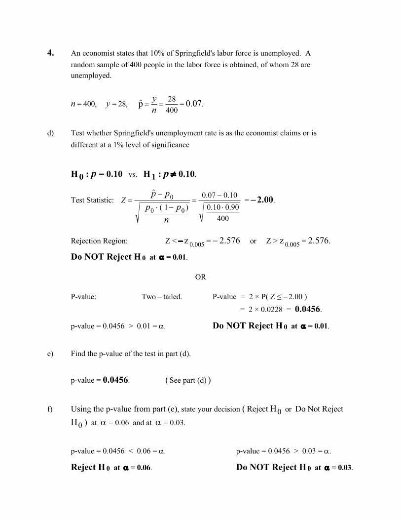
4. An economist states that 10% of Springfield's labor force is unemployed. A random sample of 400 people in the labor force is obtained, of whom 28 are unemployed.

n = 400, y = 28, = 0.07.

d) Test whether Springfield's unemployment rate is as the economist claims or is different at a 1% level of significance H 0 : p = 0.10 vs. H 1 : p ¹ 0.10.

Test Statistic: = – 2.00.

Rejection Region: Z < - z 0.005 = - 2.576 or Z > z 0.005 = 2.576.

Do NOT Reject H 0 at a = 0.01.

OR P-value: Two – tailed. P-value = 2 × P( Z ≤ – 2.00 ) = 2 × 0.0228 = 0.0456. p-value = 0.0456 > 0.01 = a. Do NOT Reject H 0 at a = 0.01. e) Find the p-value of the test in part (d). p-value = 0.0456. ( See part (d) ) f) Using the p-value from part (e), state your decision ( Reject H 0 or Do Not Reject H 0 ) at a = 0.06 and at a = 0.03. p-value = 0.0456 < 0.06 = a. p-value = 0.0456 > 0.03 = a.

Reject H 0 at a = 0.06. Do NOT Reject H 0 at a = 0.03.

40028p̂ ==

ny

40090.010.0

10.007.0)1( 00

0ˆ×

-=

-×

-=

npp

pp

Z

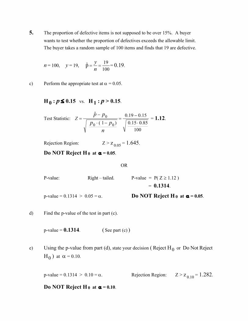
5. The proportion of defective items is not supposed to be over 15%. A buyer wants to test whether the proportion of defectives exceeds the allowable limit. The buyer takes a random sample of 100 items and finds that 19 are defective.

n = 100, y = 19, = 0.19.

c) Perform the appropriate test at a = 0.05. H 0 : p £ 0.15 vs. H 1 : p > 0.15.


Rejection Region: Z > z 0.05 = 1.645.


OR P-value: Right – tailed. P-value = P( Z ³ 1.12 )

= 0.1314. p-value = 0.1314 > 0.05 = a. Do NOT Reject H 0 at a = 0.05. d) Find the p-value of the test in part (c). p-value = 0.1314. ( See part (c) ) e) Using the p-value from part (d), state your decision ( Reject H 0 or Do Not Reject H 0 ) at a = 0.10. p-value = 0.1314 > 0.10 = a. Rejection Region: Z > z 0.10 = 1.282.


10019p̂ ==

ny

10085.015.0

15.019.0)1( 00

0ˆ×

-=

-×

-=

npp

pp

Z

6. A coffee machine is regulated so that the amount of coffee dispensed is normally distributed. A random sample of 17 cups is given below: 8.15 7.93 8.04 7.80 8.02 7.92 8.18 7.65 7.73 8.15 7.68 7.85 7.97 7.70 7.75 7.87 8.08

Recall: = 7.91, s = 0.175.

c) The coffee machine manufacturer claims that the overall average amount of coffee dispensed is at least 8 ounces. Use a = 0.05 to perform the appropriate test. State the null and alternative hypothesis for this test in terms of the relevant parameter, report the value of the test statistic, the critical value(s), and state your decision. Claim : µ ³ 8 ( the overall average amount of coffee dispensed is at least 8 ounces )

H 0 : µ ³ 8 vs. H 1 : µ < 8. Left - tailed.

s is unknown. Test Statistic: = -2.120.

n - 1 = 17 - 1 = 16 degrees of freedom. Rejection Region: T < – t 0.05 ( 16 ) = – 1.746. The value of the test statistic is in the Rejection Region. Reject H 0 at a = 0.05. d) Find the p-value (approximately) of the test in part (c). P-value = left tail. Area to the right of 2.120 is 0.025. P-value = ( Area to the left of T = - 2.120 ) = 0.025.

x

17175.0

891.7XT

0

sµ -

=-

=

n

7. A random sample of 144 patients, suffering from a particular disease are given a new medicine. 108 of the patients report an improvement in their condition. g) The company that manufactures this medicine claims 80% improvement rate. We suspect that it is less than 80%. Use a = 0.05 to perform the appropriate test. State the null and alternative hypothesis for this test in terms of the relevant parameter, report the value of the test statistic, the critical value(s), and state your decision. H 0 : p ³ 0.80 vs. H 1 : p < 0.80.

X = 108. n = 144. = 0.75.

Test Statistic: Z = = – 1.50.

Rejection Region: Z < - z 0.05 = - 1.645.

Do NOT Reject H 0 at a = 0.05. Recall: Practice Problems 10 Problem 6 (e) & (f): e) Construct a 95% confidence upper bound for the overall improvement rate.

( 0 , 0.81 )

f) The company that manufactures this medicine claims an 80% improvement rate. Based on your answer to part (e), do you find this claim believable? Explain your answer. Based on the information in our sample and part (e), values as high as 81% are reasonable candidates for the value of the (unknown) overall improvement rate of this medicine. Therefore, the manufacturer’s claim that this rate is 80% is believable. h) Find the p-value (approximately) of the test in part (g). P-value: Left – tailed. P-value = P( Z £ – 1.50 ) = 0.0668.

144108Xˆ ==

np

( )144

200800

8007501 00

0....

npp

pp̂××-

=-

-

÷÷

ø

ö

çç

è

æ -+

××nppp )ˆ(ˆzˆ 1

α , 0 ÷÷ø

öççè

æ+ ×

144)250)(750( 6451 750 , 0 ....

8. Suppose that 36% of the high schools students in a particular school district tried smoking last year. This year, a series of negative commercials about teen smoking was shown on all local TV channels. While the majority of the local community thinks the commercials helped reduce the proportion of high school students who smoke, some members of the community claim that the commercials just peak students’ curiosity about smoking and thus increase the proportion of students who smoke. In a random sample of 225 high school students, 72 tried smoking this year. a) Construct a 95% confidence interval for p, the overall proportion of students who tried smoking this year.

n = 225. x = 72. = 0.32.

The confidence interval : .

a = 0.05. a/2 = 0.025. z a/2 = 1.960.

0.32 ± 0.061 ( 0.259 , 0.381 )

b) We wish to test H 0 : p = 0.36 vs. H 1 : p ¹ 0.36. Find the p-value for this test.

= – 1.25.

p - value = two tails = 2 × P( Z < – 1.25 ) = 2 × 0.1056 = 0.2112.

22572Xˆ ==

np

nppp )ˆ1(ˆzˆ 2

-××± a

225)68.0()32.0( 960.132.0 ×

± ×

22564.036.036.032.0

)1(Z

00

0

ˆ××-

=-

-=

npp

pp

9. Several employees of Al’s Building Construction complain that the variance of the employees’ monthly salary amounts is too large. In a random sample of 10 employees, the sample standard deviation of the monthly salary amounts was $210. a) Use a = 0.05 to test H 0 : s £ 150 vs. H 1 : s > 150. Report the value of the test statistic, the critical value(s), and state your decision. s = 210. n = 10.



a = 0.05 = 16.92.

Reject H 0 if > 16.92. The value of the test statistic does fall into the Rejection Region.

Reject H 0 at a = 0.05. b) Using the chi-square distribution table only, what is the p-value of the test in part (a) ? ( You may give a range. ) 19.02 > 17.64 > 16.92 0.025 < p-value < 0.05. c) Use a computer to find the p-value of the test in part (a). =CHIDIST(17.64,9) > 1-pchisq(17.64,9) 0.039587 [1] 0.03958748

( ) ( )2

2

2 0

22

150

2101101

σsχ ×× -

=-

=n

22a> cc

2050.c

2c

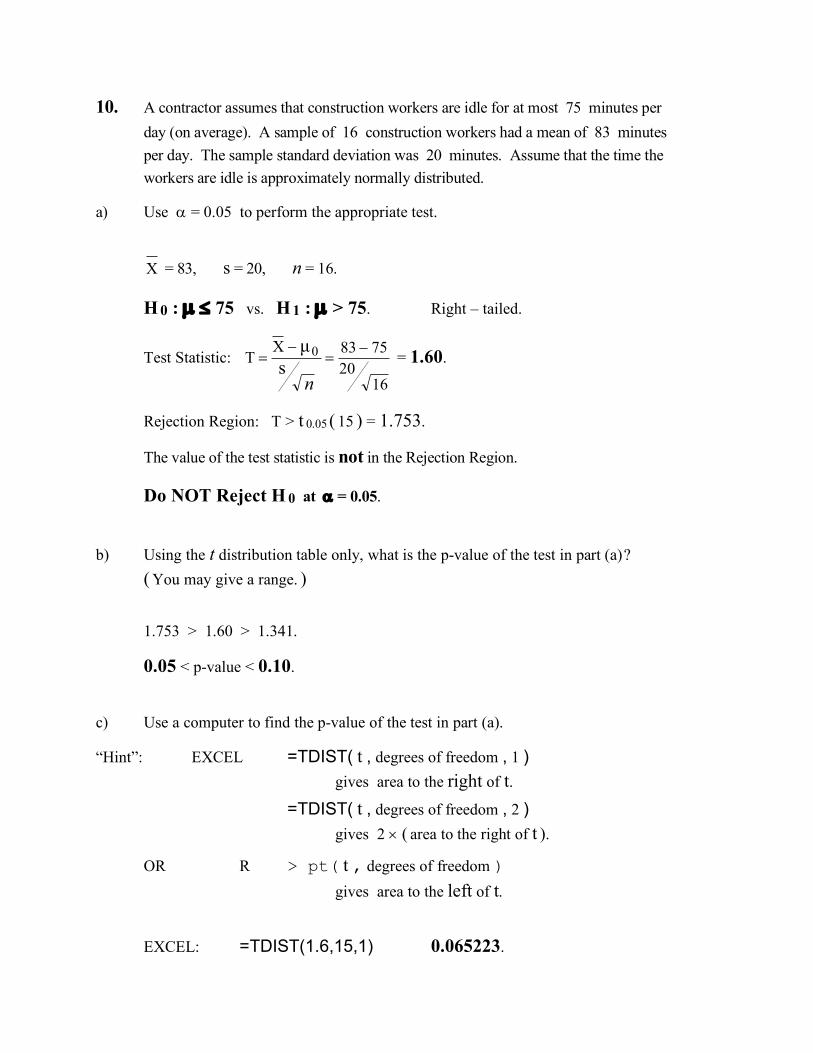
10. A contractor assumes that construction workers are idle for at most 75 minutes per day (on average). A sample of 16 construction workers had a mean of 83 minutes per day. The sample standard deviation was 20 minutes. Assume that the time the workers are idle is approximately normally distributed. a) Use a = 0.05 to perform the appropriate test. = 83, s = 20, n = 16. H 0 : µ £ 75 vs. H 1 : µ > 75. Right – tailed.


Rejection Region: T > t 0.05 ( 15 ) = 1.753. The value of the test statistic is not in the Rejection Region. Do NOT Reject H 0 at a = 0.05. b) Using the t distribution table only, what is the p-value of the test in part (a) ? ( You may give a range. ) 1.753 > 1.60 > 1.341. 0.05 < p-value < 0.10. c) Use a computer to find the p-value of the test in part (a). “Hint”: EXCEL =TDIST( t , degrees of freedom , 1 ) gives area to the right of t. =TDIST( t , degrees of freedom , 2 ) gives 2 ´ ( area to the right of t ). OR R > pt( t , degrees of freedom ) gives area to the left of t. EXCEL: =TDIST(1.6,15,1) 0.065223.

X

16 20

7583

XT

sµ0 -

=-

=

n

11. The service time in queues should not have a large variance; otherwise, the queue tends to build up. A bank regularly checks the service times of its tellers to determine their variance. A random sample of 22 service times (in minutes) gives s

2 = 8. Assume the service times are normally distributed.

a) Find a 95% confidence interval for the overall variance of service time at the bank. s

2 = 8. n = 22.

The confidence interval : .

95% confidence level a = 0.05 = 0.025.

n – 1 = 21 degrees of freedom.

= 35.48. = 10.28.

( 4.735 , 16.34 )

b) Find the two one-sided 95% confidence intervals for the overall variance of service time at the bank.

= 32.67. = 11.59.

( 5.14 , ¥ ) ( 0 , 14.5 )

( ) ( )

÷÷÷÷

ø

ö

çççç

è

æ--

-

×× 1 , 1 2

21

2 2

2

2

αα χs

χs nn

a2

20250

2

2

.cc =a

29750

2

21 .cc =a-

( ) ( )÷øö

çèæ -- ××

28.108 122 ,

48.358 122

( )÷÷ø

öççè

æ - ¥× , 12

2

αχs n ( )

÷÷ø

öççè

æ -

-

×21

2

αχs 1 , 0 n

205.0

2 χχα = 295.0

21

χχ α =-

( )÷øö

çèæ - ¥× ,

67.328 122 ( )

÷øö

çèæ - ×

59.118 122 ,0

c) Test H 0 : s 2 = 5 vs. H 1 : s

2 > 5 at a 5% level of significance.

s 2 = 8. n = 22.



a = 0.05 = 32.67.

Reject H 0 if > 32.67. The value of the test statistic does fall into the Rejection Region.

Reject H 0 at a = 0.05.

d) Using the Chi-Square distribution table only, what is the p-value of the test in part (c) ? ( You may give a range. )

35.48 > 33.6 > 32.67 0.025 < p-value < 0.05.

e) Use a computer to find the p-value of the test in part (c). “Hint”: EXCEL =CHIDIST( x , degrees of freedom ) gives area to the right of x. OR R > pchisq( x , degrees of freedom ) gives area to the left of x.

EXCEL: =CHIDIST(33.6,21) 0.039973.

( ) ( )5

812212

0

22

σsχ ×× -

=-

=n

22a> cc

2050.c

2c

12. The label on 1-gallon can of paint states that the amount of paint in the can is sufficient to paint at least 350 square feet (on average). Suppose the amount of coverage is approximately normally distributed, and the overall standard deviation of the amount of coverage is 32 square feet. A random sample of 16 cans yields the sample mean amount of coverage of 338 square feet. We wish to test H 0 : µ = 350 against H 1 : µ < 350.

a) Find the p-value for the test.

Test Statistic: = - 1.50.

P - value = P( Z ≤ - 1.50 ) = F ( - 1.50 ) = 0.0668. b) Find the Rejection Region for the test at a = 0.05. That is, for which values of the sample mean should we reject H 0 , if a 5% level of significance is used? Rejection Region:

Z = < – z a . Z = < – 1.645.

= 336.84.

c) State your decision, Reject H 0 or Do NOT Reject H 0 , at a = 0.05. = 338 > 336.84. Z = – 1.50 > – 1.645. p-value = 0.0668 > 0.05 = a. Do NOT Reject H 0 at a = 0.05.

1632

350338XZ

σµ0 -

=-

=

n

X

n σµ0X -

16 32

350X -

1632645.1350X ×-<

x

13. In a highly publicized study, doctors claimed that aspirin seems to help reduce heart attacks rate. Suppose a group of 400 men from a particular age group took an aspirin tablet three times per week. After three years, 56 of them had had heart attacks. Let p denote the overall proportion of men (in this age group) who take aspirin that have heart attacks in a 3-year period.

n = 400, x = 56, = 0.14.

d) Find the p-value of the test H 0 : p ³ 0.17 vs. H 1 : p < 0.17. Test Statistic:

= – 1.60.

Left – tailed test.

P-value = area to the left of the

test statistic. P( Z £ – 1.60 ) = 0.0548.

e) Using the p-value from part (d), state your decision ( Reject H 0 or Do Not Reject H 0 ) for a = 0.05. p - value > a Þ Do NOT Reject H 0

p - value < a Þ Reject H 0

Since 0.0548 > 0.05, Do NOT Reject H 0 at a = 0.05.

40056ˆ ==

nxp

40083.017.017.014.0

)1(Z

00

0ˆ×

-=

-×

-=

npp

pp

f) Suppose that the true proportion of all aspirin-taking men in this age group who would have a heart attack over the next 3 years is 0.15. Then in part (e) [ Type I Error, Type II Error, correct decision ] was made. ( Choose one and justify your answer. ) If p = 0.15, H 0 is false. In part (e), H 0 was NOT rejected. Therefore, a Type II Error was made. 14. Let X 1 , X 2 , … , X n be a random sample from the distribution with probability density function

, 0 < x < q, q > 0.

Find a method of moments estimator of q, .

E ( X ) = =

= = .

= Þ = .

( ) ( ) θθ

θ 12; 24

xxxf -=

θ~

( )ò -×θ

0

24 12

θθ

dxxxx ( )ò -

θ

0

43 4 12

θ

θdxxx

÷÷ø

öççè

æ-

54 12 54

4

θθ

xx5

3θ

53θ~ X θ~

3X5

15. Let g > 1 and let X 1 , X 2 , … , X n be a random sample of size n from the distribution with probability density function

f ( x ; g ) = , x > 1, zero otherwise.

Find the maximum likelihood estimator of g. Suppose n = 3, and x 1 = 2, x 2 = 2.5, x 3 = 4.

Find the maximum likelihood estimate of g.

( ) ( )γ 6

ln 1 34 γx

x-

γ̂

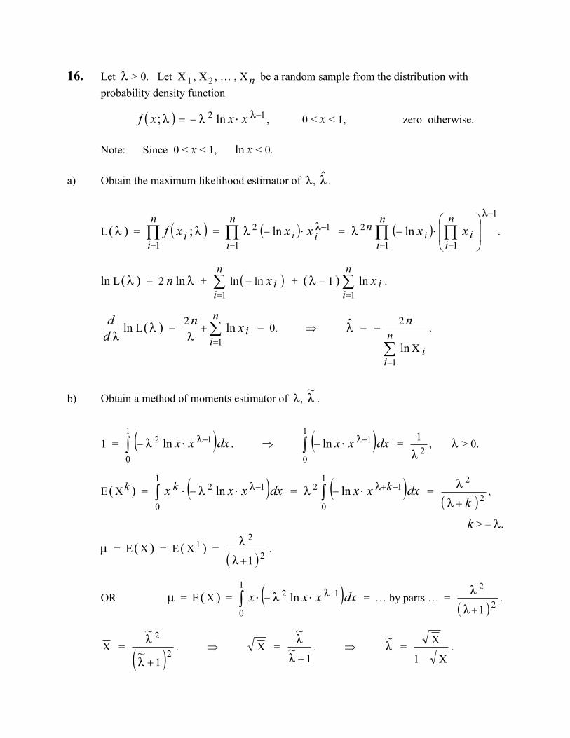
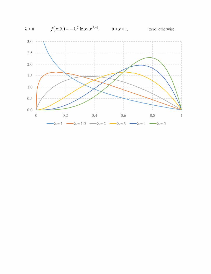
16. Let l > 0. Let X 1 , X 2 , … , X n be a random sample from the distribution with probability density function , 0 < x < 1, zero otherwise. Note: Since 0 < x < 1, ln x < 0. a) Obtain the maximum likelihood estimator of l, .

L ( l ) = = = .

ln L ( l ) = 2 n ln l + + ( l – 1 ) .

ln L ( l ) = = 0. Þ = .

b) Obtain a method of moments estimator of l, .

1 = . Þ = , l > 0.

E ( X k ) = = = ,

k > – l.

µ = E ( X ) = E ( X 1 ) = .

OR µ = E ( X ) = = … by parts … = .

= . Þ = . Þ = .

( ) 12 λ lnλλ; -×-= xxxf

λ̂

( )Õ=

n

iixf

1 λ;

( )Õ

=

-×-n

iixx i

1

12 λ

ln λ ( )

1

1

1 2

λ

ln λ

-

==÷÷

ø

ö

çç

è

æ- ÕÕ ×

n

ii

n

i

n xx i

( )å=

-n

iix

1 nn ll å

=

n

iix

1 ln

λ dd å

=+n

iix

n1

ln 2

λλ̂

å=

-n

ii

n

1

X

2

ln

λ~

( )ò -×-1

0

12 λ lnλ dxxx ( )ò -×-1

0

1 λ ln dxxx2 λ

1

( )ò -×× -1

0

12 λ lnλ dxxxx k ( )ò -+×-1

0

1 2 λ lnλ dxxx k( )2

2

λλk+

( ) 2

2

1λλ+

( )ò -×× -1

0

12 λ lnλ dxxxx( ) 2

2

1λλ+

X( )2

2

1λ~λ~

+X

1λ~λ~

+λ~

X1

X

-

For fun: .

= . Þ = . Þ = .

OR

E ( ) = = = l.

= = = .

c) Suppose n = 4, and x 1 = 0.4, x 2 = 0.7, x 3 = 0.8, x 4 = 0.9.

Obtain the maximum likelihood estimate of l, ,

and a method of moments estimator of l, .

» – 1.60147. » 4.9954.

= 0.70. » 5.1222.

å=

=n

ikin

k1

X 1

X

k X( )2

2

λ~λ~

k+k X

k+λ~λ~ λ~

k

kk

X1

X

-

X1ln-

( )ò -×× --

1

0

12 λ 1 lnln

λ dxxxx ò -

1

0

12 λ λ dxx

λ̂~ X

1 ln- å

= -

n

i in 1 X1 1

ln å=

n

ii

n 1 X

11 1

ln

λ̂

λ~

å=

n

iix

1 ln λ̂

x λ~

l > 0 , 0 < x < 1, zero otherwise.

( ) 12 λ lnλλ; -×-= xxxf

17. Let X and Y have the joint probability density function

f ( x, y ) = ,

y > 2, x > 3 y, zero otherwise. a) Sketch the support of ( X , Y ). That is, sketch { y > 2, x > 3 y }.

b) Find the value of C that would make f ( x, y ) is a valid joint p.d.f.

1 = = =

= = . Þ C = 162.

c) Set up the integral(s) for P ( X + Y > 16 ).

+

+

1 –

4

C yx

4

2 3 y

C y dx dyx

¥ ¥æ öç ÷ç ÷è ø

ò ò

3 3 2

3

xx y

C y dyx

¥ =

=

¥æ ö-ç ÷è ø

ò 2

2 81

C dyy

¥

ò

2

81yy

Cy

=

=

¥æ ö-ç ÷è ø 162

C

ò ò÷÷÷

ø

ö

ççç

è

æ

-

14

12

3

16

4

162

dxdy

xyx

xò ò¥

÷÷÷

ø

ö

ççç

è

æ

14

3

2

4

162

dxdy

xyx

ò ò ÷÷÷

ø

ö

ççç

è

æ ¥

-

4

2 16

4

162

dydxxy

yò ò¥

÷÷÷

ø

ö

ççç

è

æ ¥

4 3

4

162

dydx

xy

y

ò ò ÷÷÷

ø

ö

ççç

è

æ -4

2

16

3

4

162

dydxxyy

y

d) Set up the integral(s) for

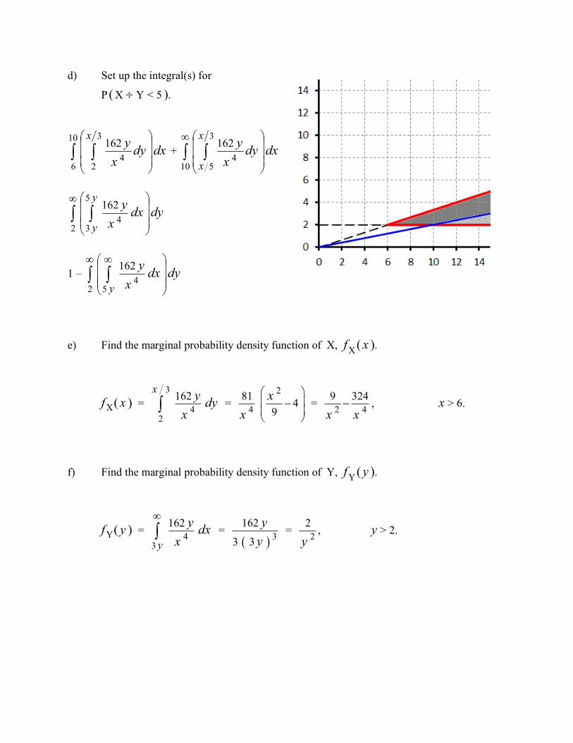
P ( X ÷ Y < 5 ).

+

1 –

e) Find the marginal probability density function of X, f X ( x ).

f X ( x ) = = = , x > 6.

f) Find the marginal probability density function of Y, f Y ( y ).

f Y ( y ) = = = , y > 2.

ò ò÷÷÷

ø

ö

ççç

è

æ10

6

3

2

4

162

dxdyxyx

ò ò¥

÷÷÷

ø

ö

ççç

è

æ

10

3

5

4

162

dxdyxyx

x

ò ò¥

÷÷÷

ø

ö

ççç

è

æ

2

5

34

162

dydxxyy

y

ò ò¥

÷÷÷

ø

ö

ççç

è

æ ¥

2 54

162

dydxxy

y

3 4

2

162x y dyxò

2

481 4

9x

x

æ öç ÷-ç ÷è ø

2 49 324

x x-

4

3

162

y

y dxx

¥

ò ( )

3

162

3 3

yy 2

2

y

Documents

4.4 3.7 5.1 4.3 4.7 3.7 3.5 4.6 4 - daviddalpiaz.github.io · STAT 400 Discussion 12 Solutions Spring 2018 1. NA random sample of size n = 9 from a normal (µ, s 2) distribution is