4 Perceptron Learning - Freie Universität€¦ · R. Rojas: Neural Networks, Springer-Verlag, Berlin, 1996 4 Perceptron Learning 4.1 Learning algorithms for neural networks In the

R. Rojas: Neural Networks, Springer-Verlag, Berlin, 1996

4

Perceptron Learning

4.1 Learning algorithms for neural networks

In the two preceding chapters we discussed two closely related models,McCulloch–Pitts units and perceptrons, but the question of how to find theparameters adequate for a given task was left open. If two sets of points haveto be separated linearly with a perceptron, adequate weights for the comput-ing unit must be found. The operators that we used in the preceding chapter,for example for edge detection, used hand customized weights. Now we wouldlike to find those parameters automatically. The perceptron learning algorithmdeals with this problem.

A learning algorithm is an adaptive method by which a network of com-puting units self-organizes to implement the desired behavior. This is done insome learning algorithms by presenting some examples of the desired input-output mapping to the network. A correction step is executed iteratively untilthe network learns to produce the desired response. The learning algorithmis a closed loop of presentation of examples and of corrections to the networkparameters, as shown in Figure 4.1.

network

test input-outputexamples

compute theerror

fix network parameters

Fig. 4.1. Learning process in a parametric system

R. Rojas: Neural Networks, Springer-Verlag, Berlin, 1996R. Rojas: Neural Networks, Springer-Verlag, Berlin, 1996


78 4 Perceptron Learning

In some simple cases the weights for the computing units can be foundthrough a sequential test of stochastically generated numerical combinations.However, such algorithms which look blindly for a solution do not qualify as“learning”. A learning algorithm must adapt the network parameters accord-ing to previous experience until a solution is found, if it exists.

4.1.1 Classes of learning algorithms

Learning algorithms can be divided into supervised and unsupervised meth-ods. Supervised learning denotes a method in which some input vectors arecollected and presented to the network. The output computed by the net-work is observed and the deviation from the expected answer is measured.The weights are corrected according to the magnitude of the error in the waydefined by the learning algorithm. This kind of learning is also called learningwith a teacher, since a control process knows the correct answer for the set ofselected input vectors.

Unsupervised learning is used when, for a given input, the exact numericaloutput a network should produce is unknown. Assume, for example, that somepoints in two-dimensional space are to be classified into three clusters. For thistask we can use a classifier network with three output lines, one for each class(Figure 4.2). Each of the three computing units at the output must specializeby firing only for inputs corresponding to elements of each cluster. If one unitfires, the others must keep silent. In this case we do not know a priori whichunit is going to specialize on which cluster. Generally we do not even knowhow many well-defined clusters are present. Since no “teacher” is available,the network must organize itself in order to be able to associate clusters withunits.

cluster 1

cluster 2

cluster 3

networkx

yx

y

•• •

• •• •

• ••

Fig. 4.2. Three clusters and a classifier network

Supervised learning is further divided into methods which use reinforce-ment or error correction. Reinforcement learning is used when after each pre-sentation of an input-output example we only know whether the networkproduces the desired result or not. The weights are updated based on thisinformation (that is, the Boolean values true or false) so that only the input



4.1 Learning algorithms for neural networks 79

vector can be used for weight correction. In learning with error correction, themagnitude of the error, together with the input vector, determines the magni-tude of the corrections to the weights, and in many cases we try to eliminatethe error in a single correction step.

learning

supervised learning

unsupervised learning

corrective learning

reinforcement learning

Fig. 4.3. Classes of learning algorithms

The perceptron learning algorithm is an example of supervised learningwith reinforcement. Some of its variants use supervised learning with errorcorrection (corrective learning).

4.1.2 Vector notation

In the following sections we deal with learning methods for perceptrons.To simplify the notation we adopt the following conventions. The input(x1, x2, . . . , xn) to the perceptron is called the input vector. If the weightsof the perceptron are the real numbers w1, w2, . . . , wn and the threshold isθ, we call w = (w1, w2, . . . , wn, wn+1) with wn+1 = −θ the extended weightvector of the perceptron and (x1, x2, . . . , xn, 1) the extended input vector. Thethreshold computation of a perceptron will be expressed using scalar products.The arithmetic test computed by the perceptron is thus

w · x ≥ θ ,

if w and x are the weight and input vectors, and

w · x ≥ 0

if w and x are the extended weight and input vectors. It will always be clearfrom the context whether normal or extended vectors are being used.

If, for example, we are looking for the weights and threshold needed toimplement the AND function with a perceptron, the input vectors and theirassociated outputs are

(0, 0) 7→ 0,(0, 1) 7→ 0,(1, 0) 7→ 0,(1, 1) 7→ 1.




If a perceptron with threshold zero is used, the input vectors must be extendedand the desired mappings are

(0, 0, 1) 7→ 0,(0, 1, 1) 7→ 0,(1, 0, 1) 7→ 0,(1, 1, 1) 7→ 1.

A perceptron with three still unknown weights (w1, w2, w3) can carry out thistask.

4.1.3 Absolute linear separability

The proof of convergence of the perceptron learning algorithm assumes thateach perceptron performs the test w · x > 0. So far we have been workingwith perceptrons which perform the test w · x ≥ 0. We must just show thatboth classes of computing units are equivalent when the training set is finite,as is always the case in learning problems. We need the following definition.

Definition 3. Two sets A and B of points in an n-dimensional space arecalled absolutely linearly separable if n + 1 real numbers w1, . . . , wn+1 existsuch that every point (x1, x2, . . . , xn) ∈ A satisfies

∑ni=1 wixi > wn+1 and

every point (x1, x2, . . . , xn) ∈ B satisfies∑n

i=1 wixi < wn+1

If a perceptron with threshold zero can linearly separate two finite setsof input vectors, then only a small adjustment to its weights is needed toobtain an absolute linear separation. This is a direct corollary of the followingproposition.

Proposition 7. Two finite sets of points, A and B, in n-dimensional spacewhich are linearly separable are also absolutely linearly separable.

Proof. Since the two sets are linearly separable, weights w1, . . . , wn+1 existfor which, without loss of generality, the inequality

n∑

i=1

wiai ≥ wn+1

holds for all points (a1, . . . , an) ∈ A and

n∑

i=1

wibi < wn+1

for all points (b1, . . . , bn) ∈ B. Let ε = max{∑ni=1 wibi − wn+1|(b1, . . . , bn) ∈

B}. It is clear that ε < ε/2 < 0. Let w′ = wn+1 + ε/2. For all points in A itholds that




n∑

i=1

wiai − (w′ − 1

2ε) ≥ 0.

This means that

n∑

i=1

wiai − w′ ≥ −1

2ε > 0⇒

n∑

i=1

wiai > w′. (4.1)

For all points in B a similar argument holds since

n∑

i=1

wibi − wn+1 =

n∑

i=1

wibi − (w′ − 1

2ε) ≤ ε,

and from this we deduce

n∑

i=1

wibi − w′ ≤ 1

2ε < 0. (4.2)

Equations (4.1) and (4.2) show that the sets A and B are absolutely linearlyseparable. If two sets are linearly separable in the absolute sense, then theyare, of course, linearly separable in the conventional sense. 2

4.1.4 The error surface and the search method

A usual approach for starting the learning algorithm is to initialize the networkweights randomly and to improve these initial parameters, looking at each stepto see whether a better separation of the training set can be achieved. In thissection we identify points (x1, x2, . . . , xn) in n-dimensional space with thevector x with the same coordinates.

Definition 4. The open (closed) positive half-space associated with the n-dimensional weight vector w is the set of all points x ∈ IRn for which w ·x > 0(w ·x ≥ 0). The open (closed) negative half-space associated with w is the setof all points x ∈ IRn for which w · x < 0 (w · x ≤ 0).

We omit the adjectives “closed” or “open” whenever it is clear from thecontext which kind of linear separation is being used.

Let P and N stand for two finite sets of points in IRn which we want toseparate linearly. A weight vector is sought so that the points in P belong to itsassociated positive half-space and the points in N to the negative half-space.The error of a perceptron with weight vector w is the number of incorrectlyclassified points. The learning algorithm must minimize this error functionE(w). One possible strategy is to use a local greedy algorithm which worksby computing the error of the perceptron for a given weight vector, lookingthen for a direction in weight space in which to move, and updating theweight vector by selecting new weights in the selected search direction. Wecan visualize this strategy by looking at its effect in weight space.




1

w1x1

w2x2

Fig. 4.4. Perceptron with constant threshold

Let us take as an example a perceptron with constant threshold θ = 1(Figure 4.4). We are looking for two weights, w1 and w2, which transformthe perceptron into a binary AND gate. We can show graphically the errorfunction for all combinations of the two variable weights. This has been donein Figure 4.5 for values of the weights between −0.5 and 1.5. The solutionregion is the triangular area in the middle. The learning algorithm shouldreach this region starting from any other point in weight space. In this case, itis possible to descend from one surface to the next using purely local decisionsat each point.

0

1 w10

1

w2

0

1

2

error

0

1 w10

1

w2

0

1

2

error

Fig. 4.5. Error function for the AND function

Figure 4.6 shows the different regions of the error function as seen from“above”. The solution region is a triangle with error level 0. For the otherregions the diagram shows their corresponding error count. The figure illus-trates an iterative search process that starts at w0, goes through w1, w2, andfinally reaches the solution region at w∗. Later on, this visualization will helpus to understand the computational complexity of the perceptron learningalgorithm.

The optimization problem we are trying to solve can be understood asdescent on the error surface but also as a search for an inner point of thesolution region. Let N = {(0, 0), (1, 0), (0, 1)} and P = {(1, 1)} be two sets ofpoints to be separated absolutely. The set P must be classified in the positive




0

1

1

1

2

2

2

w0w1

w2w∗

w1

w2

Fig. 4.6. Iteration steps to the region of minimal error

and the set N in the negative half-space. This is the separation correspondingto the AND function.

Three weights w1, w2, and w3 = −θ are needed to implement the desiredseparation with a generic perceptron. The first step is to extend the inputvectors with a third coordinate x3 = 1 and to write down the four inequalitiesthat must be fulfilled:

(0, 0, 1) · (w1, w2, w3) < 0 (4.3)

(1, 0, 1) · (w1, w2, w3) < 0 (4.4)

(0, 1, 1) · (w1, w2, w3) < 0 (4.5)

(1, 1, 1) · (w1, w2, w3) > 0 (4.6)

These equations can be written in the following simpler matrix form:

0 0 −1−1 0 −1

0 −1 −11 1 1

w1

w2

w3

>

0000

. (4.7)

This can be written asAw > 0.

where A is the 4×3 matrix of Equation (4.7) and w the weight vector (writtenas a column vector). The learning problem is to find the appropriate weightvector w.

Equation (4.7) describes all points in the interior of a convex polytope.The sides of the polytope are delimited by the planes defined by each of theinequalities (4.3)–(4.6). Any point in the interior of the polytope represents asolution for the learning problem.




We saw that the solution region for the AND function has a triangu-lar shape when the threshold is fixed at 1. In Figure 4.7 we have a three-dimensional view of the whole solution region when the threshold (i.e., w3) isallowed to change. The solution region of Figure 4.5 is just a cut of the so-lution polytope of Figure 4.7 at w3 = −1. The shaded surface represents thepresent cut, which is similar to any other cut we could make to the polytopefor different values of the threshold.

-1

w1

w2

w3

Fig. 4.7. Solution polytope for the AND function in weight space

We can see that the polytope is unbounded in the direction of negativew3. This means that the absolute value of the threshold can become as largeas we want and we will still find appropriate combinations of w1 and w2 tocompute the AND function. The fact that we have to look for interior pointsof polytopes for the solution of the learning problem, is an indication thatlinear programming methods could be used. We will elaborate on this idealater on.

4.2 Algorithmic learning

We are now in a position to introduce the perceptron learning algorithm. Thetraining set consists of two sets, P and N , in n-dimensional extended inputspace. We look for a vector w capable of absolutely separating both sets, sothat all vectors in P belong to the open positive half-space and all vectors inN to the open negative half-space of the linear separation.

Algorithm 4.2.1 Perceptron learning



4.2 Algorithmic learning 85

start: The weight vector w0 is generated randomly,set t := 0

test: A vector x ∈ P ∪N is selected randomly,

if x ∈ P and wt · x > 0 go to test,if x ∈ P and wt · x ≤ 0 go to add,if x ∈ N and wt · x < 0 go to test,if x ∈ N and wt · x ≥ 0 go to subtract.

add: set wt+1 = wt + x and t := t+ 1, goto test

subtract: set wt+1 = wt − x and t := t+ 1, goto test

This algorithm [312] makes a correction to the weight vector wheneverone of the selected vectors in P or N has not been classified correctly. Theperceptron convergence theorem guarantees that if the two sets P and N arelinearly separable the vector w is updated only a finite number of times. Theroutine can be stopped when all vectors are classified correctly. The corre-sponding test must be introduced in the above pseudocode to make it stopand to transform it into a fully-fledged algorithm.

4.2.1 Geometric visualization

There are two alternative ways to visualize perceptron learning, one moreeffective than the other. Given the two sets of points P ∈ IR2 and N ∈ IR2

to be separated, we can visualize the linear separation in input space, as inFigure 4.8, or in extended input space. In the latter case we extend the inputvectors and look for a linear separation through the origin, that is, a planewith equation w1x1 + w2x2 + w3 = 0. The vector normal to this plane is theweight vector w = (w1, w2, w3). Figure 4.9 illustrates this approach.

vectors in P

vectors in N

weight vector

p1

p2

n2

n1

Fig. 4.8. Visualization in input space




1p

2p

1n

2n

weightvector

Fig. 4.9. Visualization in extended input space

We are thus looking for a weight vector w with a positive scalar productwith all the extended vectors represented by the points in P and with anegative product with the extended vectors represented by the points in N .Actually, we will deal with this problem in a more general way. Assume thatP and N are sets of n-dimensional vectors and a weight vector w must befound, such that w · x > 0 holds for all x ∈ P and w · x < 0 holds for allx ∈ N .

The perceptron learning algorithm starts with a randomly chosen vectorw0. If a vector x ∈ P is found such that w · x < 0, this means that the anglebetween the two vectors is greater than 90 degrees. The weight vector mustbe rotated in the direction of x to bring this vector into the positive half-space defined by w. This can be done by adding w and x, as the perceptronlearning algorithm does. If x ∈ N and w · x > 0, then the angle between xand w is less than 90 degrees. The weight vector must be rotated away fromx. This is done by subtracting x from w. The vectors in P rotate the weightvector in one direction, the vectors in N rotate the negative weight vector inanother. If a solution exists it can be found after a finite number of steps. Agood initial heuristic is to start with the average of the positive input vectorsminus the average of the negative input vectors. In many cases this yields aninitial vector near the solution region.

In perceptron learning we are not necessarily dealing with normalized vec-tors, so that every update of the weight vector of the form w± x rotates theweight vector by a different angle. If x ∈ P and ‖x‖ � ‖w‖ the new weightvector w + x is almost equal to x. This effect and the way perceptron learn-ing works can be seen in Figure 4.10. The initial weight vector is updatedby adding x1, x3, and x1 again to it. After each correction the weight vec-tor is rotated in one or the other direction. It can be seen that the vector wbecomes larger after each correction in this example. Each correction rotatesthe weight vector by a smaller angle until the correct linear separation hasbeen found. After the initial updates, successive corrections become smallerand the algorithm “fine tunes” the position of the weight vector. The learningrate, the rate of change of the vector w, becomes smaller in time and if we




3) After correction with

1) Initial configuration 2) After correction with

4) After correction with

x1

x2

x3

w0

w1

w2

x1

x2

x3

w0

x1

x3

x2

x1 x1

x3

x2

w3

x3 x1

Fig. 4.10. Convergence behavior of the learning algorithm

keep on training, even after the vectors have already been correctly separated,it approaches zero. Intuitively we can think that the learned vectors are in-creasing the “inertia” of the weight vector. Vectors lying just outside of thepositive region are brought into it by rotating the weight vector just enoughto correct the error.

This is a typical feature of many learning algorithms for neural networks.They make use of a so-called learning constant, which is brought to zero dur-ing the learning process to consolidate what has been learned. The perceptronlearning algorithm provides a kind of automatic learning constant which de-termines the degree of adaptivity (the so-called plasticity of the network) ofthe weights.

4.2.2 Convergence of the algorithm

The convergence proof of the perceptron learning algorithm is easier to followby keeping in mind the visualization discussed in the previous section.




Proposition 8. If the sets P and N are finite and linearly separable, theperceptron learning algorithm updates the weight vector wt a finite number oftimes. In other words: if the vectors in P and N are tested cyclically one afterthe other, a weight vector wt is found after a finite number of steps t whichcan separate the two sets.

Proof. We can make three simplifications without losing generality:

i) The sets P and N can be joined in a single set P ′ = P ∪N−, where theset N− consists of the negated elements of N .

ii) The vectors in P ′ can be normalized, because if a weight vector w is foundso that w · x > 0 this is also valid for any other vector ηx, where η is aconstant.

iii) The weight vector can also be normalized. Since we assume that a solutionfor the linear separation problem exists, we call w∗ a normalized solutionvector.

Assume that after t + 1 steps the weight vector wt+1 has been computed.This means that at time t a vector pi was incorrectly classified by the weightvector wt and so wt+1 = wt + pi.

The cosine of the angle ρ between wt+1 and w∗ is

cos ρ =w∗ ·wt+1

‖wt+1‖(4.8)

For the expression in the numerator we know that

w∗wt+1 = w∗ · (wt + pi)

= w∗ ·wt + w∗ · pi

≥ w∗ ·wt + δ

with δ = min{w∗ ·p | ∀p ∈ P ′}. Since the weight vector w∗ defines an absolutelinear separation of P and N we know that δ > 0. By induction we obtain

w∗ ·wt+1 ≥ w∗ ·w0 + (t+ 1)δ. (4.9)

On the other hand for the term in the denominator of (4.8) we know that

‖wt+1‖2 = (wt + pi) · (wt + pi)

= ‖wt‖2 + 2wt · pi + ‖pi‖2

Since wt · pi is negative or zero (otherwise we would have not corrected wt

using pi) we can deduce that

‖wt+1‖2 ≤ ‖wt‖2 + ‖pi‖2

≤ ‖wt‖2 + 1




because all vectors in P have been normalized. Induction then gives us

‖wt+1‖2 ≤ ‖w0‖2 + (t+ 1). (4.10)

From (4.9) and (4.10) and Equation (4.8) we get the inequality

cos ρ ≥ w∗ ·w0 + (t+ 1)δ√

‖w0‖2 + (t+ 1)

The right term grows proportionally to√t and, since δ is positive, it can

become arbitrarily large. However, since cos ρ ≤ 1, t must be bounded by amaximum value. Therefore, the number of corrections to the weight vectormust be finite. 2

The proof shows that perceptron learning works by bringing the initialvector w0 sufficiently close to w∗ (since cos ρ becomes larger and ρ propor-tionately smaller).

4.2.3 Accelerating convergence

Although the perceptron learning algorithm converges to a solution, the num-ber of iterations can be very large if the input vectors are not normalized andare arranged in an unfavorable way.

There are faster methods to find the weight vector appropriate for a givenproblem. When the perceptron learning algorithm makes a correction, an in-put vector x is added or subtracted from the weight vector w. The searchdirection is given by the vector x. Each input vector corresponds to the bor-der of one region of the error function defined on weight space. The directionof x is orthogonal to the step defined by x on the error surface. The weightvector is displaced in the direction of x until it “falls” into a region withsmaller error.

We can illustrate the dynamics of perceptron learning using the error sur-face for the OR function as an example. The input (1, 1) must produce theoutput 1 (for simplicity we fix the threshold of the perceptron to 1). Thetwo weights w1 and w2 must fulfill the inequality w1 + w2 ≥ 1. Any othercombination produces an error. The contribution to the total error is shownin Figure 4.11 as a step in the error surface. If the initial weight vector liesin the triangular region with error 1, it must be brought up to the verge ofthe region with error 0. This can be done by adding the vector (1,1) to w.However, if the input vector is, for example, (0.1, 0.1), it should be added afew times before the weight combination (w1, w2) falls to the region of error0. In this case we would like to make the correction in a single iteration.

These considerations provide an improvement for the perceptron learningalgorithm: if at iteration t the input vector x ∈ P is classified erroneously,then we have wt · x ≤ 0. The error δ can be defined as




(1,1)

error

(0.1,0.1)

w 1

w2

w2

w1

Fig. 4.11. A step on the error surface

δ = −wt · x.

The new weight vector wt+1 is calculated as follows:

wt+1 = wt +δ + ε

‖x‖2 x,

where ε denotes a small positive real number. The classification of x has beencorrected in one step because

wt+1 · x = (wt +δ + ε

‖x‖2 x) · x

= wt · x + (δ + ε)

= −δ + δ + ε

= ε > 0

The number ε guarantees that the new weight vector just barely skips overthe border of the region with a higher error. The constant ε should be madesmall enough to avoid skipping to another region whose error is higher thanthe current one. When x ∈ N the correction step is made similarly, but usingthe factor δ − ε instead of δ + ε.

The accelerated algorithm is an example of corrective learning: We do notjust “reinforce” the weight vector, but completely correct the error that hasbeen made. A variant of this rule is correction of the weight vector using aproportionality constant γ as the learning factor, in such a way that at eachupdate the vector γ(δ+ ε)x is added to w. The learning constant falls to zeroas learning progresses.

4.2.4 The pocket algorithm

If the learning set is not linearly separable the perceptron learning algorithmdoes not terminate. However, in many cases in which there is no perfect linear




separation, we would like to compute the linear separation which correctlyclassifies the largest number of vectors in the positive set P and the negativeset N . Gallant proposed a very simple variant of the perceptron learningalgorithm capable of computing a good approximation to this ideal linearseparation. The main idea of the algorithm is to store the best weight vectorfound so far by perceptron learning (in a “pocket”) while continuing to updatethe weight vector itself. If a better weight vector is found, it supersedes theone currently stored and the algorithm continues to run [152].




Algorithm 4.2.2 Pocket algorithm

start : Initialize the weight vector w randomly. Define a “stored” weightvector ws = w. Set hs, the history of ws, to zero.

iterate : Update w using a single iteration of the perceptron learning algo-rithm. Keep track of the number h of consecutively successfully testedvectors. If at any moment h > hs, substitute ws with w and hs withh. Continue iterating.

The algorithm can occasionally change a good stored weight vector for aninferior one, since only information from the last run of selected examples isconsidered. The probability of this happening, however, becomes smaller andsmaller as the number of iterations grows. If the training set is finite and theweights and vectors are rational, it can be shown that this algorithm convergesto an optimal solution with probability 1 [152].

4.2.5 Complexity of perceptron learning

The perceptron learning algorithm selects a search direction in weight spaceaccording to the incorrect classification of the last tested vector and does notmake use of global information about the shape of the error function. It is agreedy, local algorithm. This can lead to an exponential number of updatesof the weight vector.

w1

w2

zero error1

1

2

iterations

w0

Fig. 4.12. Worst case for perceptron learning (weight space)

Figure 4.12 shows the different error regions in a worst case scenario. Theregion with error 0 is bounded by two lines which meet at a small angle.Starting the learning algorithm at point w0, the weight updates will lead to asearch path similar to the one shown in the figure. In each new iteration a newweight vector is computed, in such a way that one of two vectors is classified



4.3 Linear programming 93

correctly. However, each of these corrections leads to the other vector beingincorrectly classified. The iteration jumps from one region with error 1 to theother one. The algorithm converges only after a certain number of iterations,which can be made arbitrarily large by adjusting the angle at which the linesmeet.

Figure 4.12 corresponds to the case in which two almost antiparallel vec-tors are to be classified in the same half-space (Figure 4.13). An algorithmwhich rotates the separation line in one of the two directions (like perceptronlearning) will require more and more time when the angle between the twovectors approaches 180 degrees.

x1

x2

Fig. 4.13. Worst case for perceptron learning (input space)

This example is a good illustration of the advantages of visualizing learningalgorithms in both the input space and its dual, weight space. Figure 4.13shows the concrete problem and Figure 4.12 illustrates why it is difficult tosolve.

4.3 Linear programming

A set of input vectors to be separated by a perceptron in a positive and anegative set defines a convex polytope in weight space, whose inner pointsrepresent all admissible weight combinations for the perceptron. The percep-tron learning algorithm finds a solution when the interior of the polytope isnot void. Stated differently: if we want to train perceptrons to classify pat-terns, we must solve an inner point problem. Linear programming can dealwith this kind of task.

4.3.1 Inner points of polytopes

Linear programming was developed to solve the following generic problem:Given a set of n variables x1, x2, . . . , xn a function c1x1+c2x2+· · ·+cnxn must




be maximized (or minimized). The variables must obey certain constraintsgiven by linear inequalities of the form

a11x1 + a12x2 + · · ·+ a1nxn ≤ b1

a21x1 + a22x2 + · · ·+ a2nxn ≤ b2...

......

am1x1 + am2x2 + · · ·+ amnxn ≤ bm

All m linear constraints can be summarized in the matrix inequality Ax ≤ b,in which x and b respectively represent n-dimensional and m-dimensionalcolumn vectors and A is a m × n matrix. It is also necessary that x ≥ 0,which can always be guaranteed by introducing additional variables.

As in the case of a perceptron, the m inequalities define a convex polytopeof feasible values for the variables x1, x2, . . . , xn. If the optimization problemhas a solution, this is found at one of the vertices of the polytope. Figure 4.14shows a two-dimensional example. The shaded polygon is the feasible region.The function to be optimized is represented by the line normal to the vector c.Finding the point where this linear function reaches its maximum correspondsto moving the line, without tilting it, up to the farthest position at which itis still in contact with the feasible region, in our case ξ. It is intuitively clearthat when one or more solutions exist, one of the vertices of the polytope isone of them.

x1

x2

c

ξ

Fig. 4.14. Feasible region for a linear optimization problem

The well-known simplex algorithm of linear programming starts at a ver-tex of the feasible region and jumps to another neighboring vertex, alwaysmoving in a direction in which the function to be optimized increases. In theworst case an exponential number of vertices in the number of inequalitiesm has to be traversed before a solution is found. On average, however, the




simplex algorithm is not so inefficient. In the case of Figure 4.14 the optimalsolution can be found in two steps by starting at the origin and moving to theright. To determine the next vertex to be visited, the simplex algorithm usesas a criterion the length of the projection of the gradient of the function tobe optimized on the edges of the polytope. It is in this sense a gradient algo-rithm. The algorithm can be inefficient because the search for the optimum isconstrained to be carried out moving only along the edges of the polytope. Ifthe number of delimiting surfaces is large, a better alternative is to go rightthrough the middle of the polytope.

4.3.2 Linear separability as linear optimization

The simplex algorithm and its variants need to start at a point in the feasibleregion. In many cases it can be arranged to start at the origin. If the feasibleregion does not contain the origin as one of its vertices, a feasible point mustbe found first. This problem can be transformed into a linear program.

Let A represent the m× n matrix of coefficients of the linear constraintsand b an m-dimensional column vector. Assume that we are looking for ann-dimensional column vector x such that Ax ≤ b. This condition is fulfilledonly by points in the feasible region. To simplify the problem, assume thatb ≥ 0 and that we are looking for vectors x ≥ 0. Introducing the columnvector y of m additional slack variables (y1, . . . , ym), the inequality Ax ≤ bcan be transformed into the equality Ax+Iy = b, where I denotes the m×midentity matrix. The linear program to be solved is then

min{m∑

i=1

yi|Ax + Iy = b,x ≥ 0,y ≥ 0}.

An initial feasible solution for the problem is x = 0 and y = b. Starting fromhere an iterative algorithm looks for the minimum of the sum of the slackvariables. If the minimum is negative the original problem does not have asolution and the feasible region of Ax ≤ b is void. If the minimum is zero, thevalue of x determined during the optimization is an inner point of the feasibleregion (more exactly, a point at its boundary).

The conditions x ≥ 0 and b ≥ 0 can be omitted and additional transfor-mations help to transform the more general problem to the canonical formdiscussed here [157].

Inner points of convex polytopes, defined by separating hyperplanes, canthus be found using linear programming algorithms. Since the computationof the weight vector for a perceptron corresponds to the computation of innerpoints of convex polytopes, this means that perceptron learning can also behandled in this way. If two sets of vectors are not linearly separable, the linearprogramming algorithm can detect it. The complexity of linearly separatingpoints in an input space is thus bounded by the complexity of solving linearprogramming problems.




The perceptron learning algorithm is not the most efficient method forperceptron learning, since the number of steps can grow exponentially in theworst case. In the case of linear programming, theoreticians have succeeded incrafting algorithms which need a polynomial number of iterations and returnthe optimal solution or an indication that it does not exist.

4.3.3 Karmarkar’s algorithm

In 1984 a fast polynomial time algorithm for linear programming was proposedby Karmarkar [236]. His algorithm starts at an inner point of the solutionregion and proceeds in the direction of steepest ascent (if maximizing), takingcare not to step out of the feasible region.

Figure 4.15 schematically shows how the algorithm works. The algorithmstarts with a canonical form of the linear programming problem in whichthe additional constraint x1 + x2 + · · · + xn = 1 is added to the basic con-straints Ax ≥ 0, where x1, . . . , xn are the variables in the problem. Somesimple transformations can bring the original problem into this form. Thepoint e = 1

n (1, 1, . . . , 1) is considered the middle of the solution polytope andeach iteration step tries to transform the original problem in such a way thatthis is always the starting point.

x1

x2

c

•

•a1

a0

′a0

′a1 •

•

T

Fig. 4.15. Transformation of the solution polytope

An initial point a0 is selected in the interior of the solution polytope andthen brought into the middle e of the transformed feasible region using aprojective transformation T . A projective transformation maps each point xin the hyperplane x1 + x2 + · · ·+ xn = 1 to a point x′ in another hyperplane,whereby the line joining x and x′ goes through a predetermined point p.The transformation is applied on the initial point a0, the matrix A of linearconstraints and also to the linear function cT x to be optimized. After the




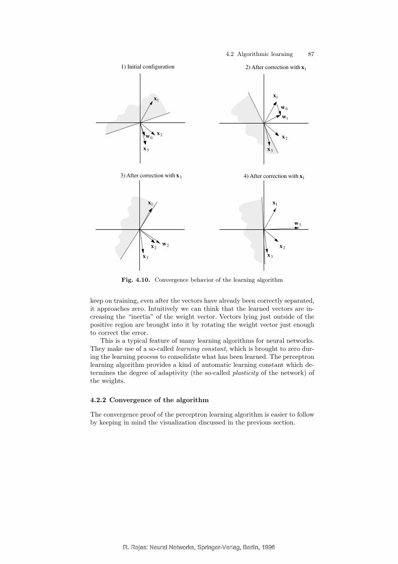
transformation, the radius of the largest sphere with center a′0 and insidethe transformed feasible region is computed. Starting at the center of thesphere a new point in the direction of the transformed optimizing directionc′ is computed. The step length is made shorter than the computed maximalradius by a small factor, to avoid reaching the surface of the solution polytope.The new point a′1 computed in this way is a feasible point and is also strictlyin the interior of the solution polytope. The point a′1 is transformed backto the original space using the inverse projective transformation T−1 and anew iteration can start again from this point. This basic step is repeated,periodically testing whether a vertex of the polytope is close enough andoptimal. At this moment the algorithm stops and takes this vertex as thesolution of the problem (Figure 4.16). Additionally, a certain checking must bedone in each iteration to confirm that a solution to the optimization problemexists and that the cost function is not unbounded.

x1

x2

ca1

a0

a2

al

Fig. 4.16. Example of a search path for Karmarkar’s algorithm

In the worst case Karmarkar’s algorithm executes in a number of iterationsproportional to n3.5, where n is the number of variables in the problem andother factors are kept constant. Some published modifications of Karmarkar’salgorithm are still more efficient but start beating the simplex method inthe average case only when the number of variables and constraints becomesrelatively large, since the computational overhead for a small number of con-straints is not negligible [257].

The existence of a polynomial time algorithm for linear programming andfor the solution of interior point problems shows that perceptron learningis not what is called a hard computational problem. Given any number oftraining patterns, the learning algorithm (in this case linear programming)can decide whether the problem has a solution or not. If a solution exists, itfinds the appropriate weights in polynomial time at most.




4.4 Historical and bibliographical remarks

The success of the perceptron and the interest it aroused in the 1960s was adirect product of its learning capabilities, different from the hand-design ap-proach of previous models. Later on, research in this field reached an impassewhen a learning algorithm for more general networks was still unavailable.

Minsky and Papert [312] analyzed the features and limitations of the per-ceptron model in a rigorous way. They could show that the perceptron learningalgorithm needs an exponential number of learning steps in the worst case.However, perceptron learning is in the average case fairly efficient. Mansfieldshowed that when the training set is selected randomly from a half-space, thenumber of iterations of the perceptron learning algorithm is comparable tothe number of iterations needed by ellipsoid methods for linear programming(up to dimension 30) [290]. Baum had previously shown that when the learn-ing set is picked by a non-malicious adversary, the complexity of perceptronlearning is polynomial [46].

More recently the question has arisen of whether a given set of nonlin-early separable patterns can be decomposed in such a way that the largestlinearly separable subset can be detected. Amaldi showed that this is an NP-complete problem, that is, a problem for which presumably no polynomialtime algorithm exists (compare Chap. 10).

The conditions for perfect perceptron learning can be also relaxed. If theset of patterns is not linearly separable, we can look for the separation thatminimizes the average quadratic error, without requiring it to be zero. In thiscase statistical methods or the backpropagation algorithm (Chap. 7) can beused.

After the invention of the simplex algorithm for linear programming therewas a general feeling that it could be proven that one of its variants was ofpolynomial complexity in the number of constraints and of variables. Thiswas due to the fact that the actual experience with the algorithm showedthat in the average case a solution was found in much less than exponentialtime. However, in 1972 Klee and Minty [247] gave a counterexample whichshowed that there were situations in which the simplex method visited 2n−1

vertices of a feasible region with 2n vertices. Later it was rigorously proventhat the simplex method is polynomial in the average case [64]. The questionof the existence of a polynomial time algorithm for linear programming wassettled by Khachiyan in 1979, when he showed that a recursive constructionof ellipsoids could lead to finding the optimal vertex of the feasible regionin polynomial time [244]. His algorithm, however, was very computationallyintensive for most of the average-sized problems and could not displace thesimplex method. Karmarkar’s algorithm, a further development of the ellip-soid method including some very clever transformations, aroused much inter-est when it was first introduced in 1984. So many variations of the originalalgorithm have appeared that they are collectively known as Karmarkar-typealgorithms. Minimization problems with thousands of constraints can now be



4.4 Historical and bibliographical remarks 99

dealt with efficiently by these polynomial time algorithms, but since the sim-plex method is fast in the average case it continues to be the method of choicein medium-sized problems.

Interesting variations of perceptron learning were investigated by Fonta-nari and Meir, who coded the different alternatives of weight updates accord-ing to the local information available to each weight and let a population ofalgorithms evolve. With this kind of “evolution strategy” they found compet-itive algorithms similar to the standard methods [140].

Exercises

1. Implement the perceptron learning algorithm in the computer. Find theweights for an edge detection operator using this program. The input-output examples can be taken from a digitized picture of an object andanother one in which only the edges of the object have been kept.

2. Give a numerical example of a training set that leads to many iterationsof the perceptron learning algorithm.

3. How many vectors can we pick randomly in an n-dimensional space sothat they all belong to the same half-space? Produce a numerical estimateusing a computer program.

4. The perceptron learning algorithm is usually fast if the vectors to belinearly separated are chosen randomly. Choose a weight vector w for aperceptron randomly. Generate p points in input space and classify themin a positive or negative class according to their scalar product with w.Now train a perceptron using this training set and measure the numberof iterations needed. Make a plot of n against p for dimension up to 10and up to 100 points.


R. Rojas: Neural Networks, Springer-Verlag, Berlin, 1996R. Rojas: Neural Networks, Springer-Verlag, Berlin, 1996R. Rojas: Neural Networks, Springer-Verlag, Berlin, 1996

Documents

4 Perceptron Learning - Freie Universität€¦ · R. Rojas: Neural Networks, Springer-Verlag, Berlin, 1996 4 Perceptron Learning 4.1 Learning algorithms for neural networks In the