Embed Size (px)
Citation preview

1
3.3 Network-Centric Community Detection
A Unified Process

2
3.3 Network-Centric Community Detection
Comparison– Spectral clustering essentially tries to minimize the number of
edges between groups.– Modularity consider the number of edges which is smaller than
expected.
– The spectral partitioning is forced to split the network into ap-proximately equal-size clusters.
3
3.4 Hierarchy-Centric Community Detection
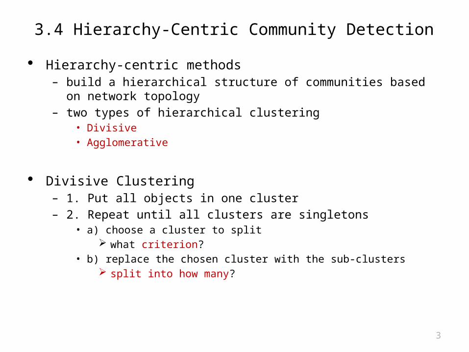
Hierarchy-centric methods– build a hierarchical structure of communities based on network
topology– two types of hierarchical clustering
• Divisive• Agglomerative
Divisive Clustering– 1. Put all objects in one cluster– 2. Repeat until all clusters are singletons
• a) choose a cluster to split what criterion?
• b) replace the chosen cluster with the sub-clusters split into how many?
4
3.4 Hierarchy-Centric Community Detection
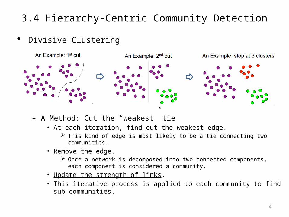
Divisive Clustering
– A Method: Cut the “weakest” tie• At each iteration, find out the weakest edge.
This kind of edge is most likely to be a tie connecting two communities.
• Remove the edge. Once a network is decomposed into two connected components, each
component is considered a community.
• Update the strength of links.• This iterative process is applied to each community to find sub-com-
munities.

5
3.4 Hierarchy-Centric Community Detection
Divisive Clustering– “Finding and evaluating community structure in
networks,” M. Newman and M. Girvan, Physical Review, 2004• find the weak ties based on “edge betweenness”• Edge betweenness
the number of shortest paths between pair of nodes pass along the edge utilized to find the “weakest” tie for hierarchical clustering
• where is the total number of shortest paths between nodes and is the number of shortest paths between nodes and that pass along the
edge .
𝐶𝐵 (𝑒(𝑣 𝑖 ,𝑣 𝑗))={ ∑𝑣𝑠 ,𝑣𝑡∈𝑉 , 𝑠<𝑡
𝜎𝑠𝑡 (𝑒(𝑣 𝑖 ,𝑣 𝑗))𝜎 𝑠𝑡
𝑖𝑓 𝑖< 𝑗
0 𝑖𝑓 𝑖= 𝑗𝐶𝐵 (𝑒(𝑣 𝑗 ,𝑣 𝑖)) 𝑖𝑓 𝑖> 𝑗

6
3.4 Hierarchy-Centric Community Detection
Divisive Clustering– The edge with higher betweenness tends to be the bridge be-
tween two communities
– It is used to progressively remove the edges with the highest be-tweenness.

7
3.4 Hierarchy-Centric Community Detection
Divisive Clustering– “Finding and evaluating community structure in
networks,” M. Newman and M. Girvan, Physical Review, 2004• Example
– Negatives for divisive clustering• edge betweenness-based scheme requires high computation• One removal of an edge will lead to the recomputation of betweenness
for all edges

8
3.4 Hierarchy-Centric Community Detection
Agglomerative Clustering– begins with base (singleton) communities– merges them into larger communities with certain criterion.
• One example criterion: modularity Let be the fraction of edges in the network that connect nodes in commu-
nity to those in community Let , then the modularity values approaching indicate networks with strong community structure values for real networks typically fall in the range from 0.3 to 0.7
동일한 Community 안의 Edge 수 – 서로 다른 Community 들 간의 Edge
수

9
3.4 Hierarchy-Centric Community Detection
Agglomerative Clustering– Two communities are merged if the merge results in the largest
increase of overall modularity– The merge continues until no merge can be found to improve the
modularity.
Dendrogram according to Agglomerative Clustering based on Modularity
10
3.4 Hierarchy-Centric Community Detection
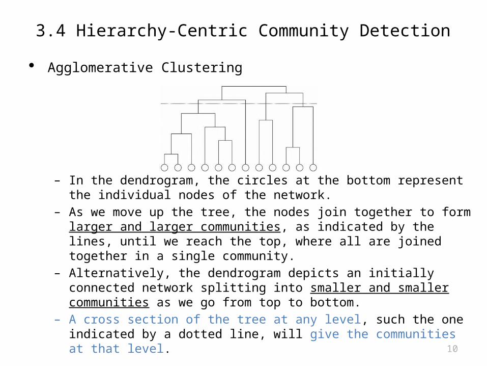
Agglomerative Clustering
– In the dendrogram, the circles at the bottom represent the indi-vidual nodes of the network.
– As we move up the tree, the nodes join together to form larger and larger communities, as indicated by the lines, until we reach the top, where all are joined together in a single community.
– Alternatively, the dendrogram depicts an initially connected net-work splitting into smaller and smaller communities as we go from top to bottom.
– A cross section of the tree at any level, such the one indicated by a dotted line, will give the communities at that level.

11
3.4 Hierarchy-Centric Community Detection
Divisive vs. Agglomerative Clustering– Zachary's karate club study
Zachary observed 34 members of a karate club over a period of two years. During the
course of the study, a disagreement de-veloped between the administrator (34) of
the club and the club's instructor (1), which ultimately resulted in the instruc-
tor's leaving and starting a new club, tak-ing about a half of the original club's
members with him

12
3.4 Hierarchy-Centric Community Detection
Divisive vs. Agglomerative Clustering
– Divisive • “Community structure in social and biological networks”,
Michelle Girvan, and M. E. J. Newman, 2001 Using edge-betweeness
– Agglomerative • “Fast algorithm for detecting community structure in networks”, M. E. J. New-
man, 2003 Using modularity
Divisive Agglomerative

13
Summary of Community Detection
Node-Centric Community Detection– cliques, k-cliques, k-clubs
Group-Centric Community Detection– quasi-cliques
Network-Centric Community Detection– Clustering based on vertex similarity– Latent space models, block models, spectral clustering,
modularity maximization
Hierarchy-Centric Community Detection– Divisive clustering– Agglomerative clustering

14
3.5 Community Evaluation Here, we consider a “Social Network with Ground Truth”
– Community membership for each actor is known an ideal case– For example,
• A synthetic networks generated based on predefined community structures L. Tang and H. Liu. “Graph mining applications to social network analysis.” In C. Ag-
garwal and H.Wang, editors, Managing and MiningGraph Data, chapter 16, pages 487.513.Springer, 2010b
• Some well-studied tiny networks like Zachary’s karate club with 34 members M.Newman. “Modularity and community structure in networks.” PNAS,
103(23):8577.8582, 2006a.
Simple comparison between the ground truth with the identified commu-nity structure– Visualization– One-to-one mapping

15
3.5 Community Evaluation The number of communities after grouping can be different
from the ground truth No clear community correspondence between clustering re-
sult and the ground truth
Normalized Mutual Information (NMI) can be used
Each number denotes a node, and each circle or block denotes a community1) Both communities {1, 3} and {2} map to the community {1, 2, 3} in the ground truth2) The node 2 is wrongly assigned
How to measure the clustering quality?

16
3.5 Community Evaluation Entropy
– 확률변수의 불확실성을 측정하기 위한 것– Measure of disorder– The information volume contained in a random variable X (or
in a distribution X)
• X 의 엔트로피는 X 의 모든 가능한 결과값 x 에 대해 x 의 발생 확률과 그 확률의 역수의 로그 값의 곱의 합
• 일반적으로 지수 b 의 값으로서 2 나 오일러의 수 e, 또는 10 이 많이 사용된다 . b=2 인 경우에는 엔트로피의 단위가 비트 (bit) 이며 , b=e 이면 네트 (nat), 그리고 b=10 인 경우에는 디짓 (digit) 이 된다 .
𝐻 ( 𝑋 )=−∑𝑥∈𝑋
𝑝 (𝑥 )𝑙𝑜𝑔𝑏(𝑥)

17
3.5 Community Evaluation Entropy 와 동전 던지기 [from wikipedia]
– 앞면과 뒷면이 나올 확률이 같은 동전을 던졌을 경우의 엔트로피를 생각해 보자 . 이는 H,T 두 가지의 경우만을 나타내므로 엔트로피는 1이다 .
– + )=1
– 한편 공정하지 않는 동전의 경우에는 특정 면이 나올 확률이 상대적으로 더 높기 때문에 엔트로피는 1 보다 작아진다 . 우리가 예측해서 맞출 수 있는 확률이 더 높아졌기 때문에 정보의 양 , 즉 엔트로피는 더 작아진 것이다 . 동전던지기의 경우에는 앞 , 뒤 면이 나올 확률이 1/2 로 같은 동전이 엔트로피가 가장 크다 .
– 엔트로피를 불확실성 (uncertainity) 과 같은 개념이라고 인식할 수 있다 .
– 불확실성이 높아질수록 정보의 양은 더 많아지고 엔트로피는 더 커진다 .

18
3.5 Community Evaluation Mutual Information ( 상호 정보량 )
– It measures the shared information volume between two ran-dom variables (or two distributions)
– 두 확률 변수 ( 또는 두 분포 ) X, Y 가 얼마나 밀접한 관계가 있는지 또는 얼마나 서로간에 의존을 하는지를 측정
– 국문 참고 문헌 • http://shineware.tistory.com/7• http://www.dbpia.co.kr/Journal/ArticleDetail/339089

19
3.5 Community Evaluation Normalized Mutual Information (NMI, 정규화된 상호 정보량 )
– It measures the shared information volume between two random variables (or two distributions)
– 두 확률 변수 ( 또는 두 분포 ) X, Y 가 얼마나 밀접한 관계가 있는지를 측정
– The values is between 0 and 1
Consider a partition as a random variable, we can compute the matching quality between ground truth and the identified clustering

20
3.5 Community Evaluation NMI Example (1/2)
– Partition a (): [1, 1, 1, 2, 2, 2] – Partition b (): [1, 2, 1, 3, 3, 3]
1, 2, 34, 5,
61, 3
2 4, 5,6
𝜋𝑎
𝜋𝑏

21
3.5 Community Evaluation NMI Example (2/2)
– Partition a (): [1, 1, 1, 2, 2, 2] – Partition b (): [1, 2, 1, 3, 3, 3]
1, 2, 34, 5,
61, 3
2 4, 5,6
𝜋𝑎
𝜋𝑏
=0.8278
ahn
bln lhn ,

22
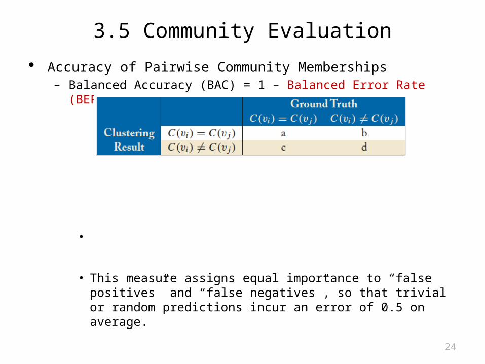
3.5 Community Evaluation Accuracy of Pairwise Community Memberships
– Consider all the possible pairs of nodes and check whether they reside in the same community
– An error occurs if• Two nodes belonging to the same community are assigned to differ-
ent communities after clustering• Two nodes belonging to different communities are assigned to the
same community
– Construct a contingency table

23
3.5 Community Evaluation Accuracy of Pairwise Community Memberships
Ground Truth
1, 2, 3
4, 5, 6
1, 3
24, 5, 6
Clustering Result
Accuracy = (4+9)/ (4+2+9+0) = 0.86
24
3.5 Community Evaluation Accuracy of Pairwise Community Memberships
– Balanced Accuracy (BAC) = 1 – Balanced Error Rate (BER)
•
• This measure assigns equal importance to “false positives” and “false negatives”, so that trivial or random predictions incur an error of 0.5 on average.

25
3.5 Community Evaluation Accuracy of Pairwise Community Memberships
– Balanced Accuracy (BAC) = 1 – Balanced Error Rate (BER)
•
0.83

26
3.5 Community Evaluation Evaluation without Ground Truth
– This is the most common situation– Quantitative evaluation functions: modularity
• Once we have a network partition, we can compute its modularity • The method with higher modularity wins
• modularity Let be the fraction of edges in the network that connect nodes in com-
munity to those in community Let , then the modularity values approaching indicate networks with strong community structure values for real networks typically fall in the range from 0.3 to 0.7
동일한 Community 안의 Edge 수 – 서로 다른 Community 들 간의 Edge
수

27
Book Available at • Morgan & claypool Publis
hers• Amazon
If you have any comments, please feel free to contact:
• Lei Tang, Yahoo! Labs, [email protected]
• Huan Liu, ASU [email protected]