Embed Size (px)
Citation preview

Sample Complexity and Uniform Convergence
Eli Upfal

Extracting Information from Data
Data science, machine learning, data mining, pattern recognition,statistical inference, ”the scientific method”,...
DATA ⇒ ALGORITHM ⇒ MODEL

Extracting Information from Data
Data science, machine learning, data mining, pattern recognition,statistical inference, ”the scientific method”,...
DATA ⇒ ALGORITHM ⇒ MODELIn CS we focus on the algorithm (efficiency, correctness withrespect to the input)
DATA ⇒ ALGORITHM ⇒ MODEL

Extracting Information from Data
Data science, machine learning, data mining, pattern recognition,statistical inference, ”the scientific method”,...
DATA ⇒ ALGORITHM ⇒ MODELIn CS we focus on the algorithm (efficiency, correctness withrespect to the input)
DATA ⇒ ALGORITHM ⇒ MODEL
but f (garbage) = garbageIn data analysis we need to verify that the information is in thedata:
DATA ⇒ ALGORITHM ⇒ MODEL

Sample Complexity
Sample Complexity addresses the fundamental questions in dataanalysis:
• Does the data (training set) contains sufficient information tomake a valid predictions (or fix a model)?
• Is the sample sufficiently large?
• How accurate is a prediction (model) inferred from a sampleof a given size?
Standard statistics/probabilistic techniques do not give adequatesoluions

Outline:
• Motivation: learning a binary classifier, the realizable andnon-realizable case.
• Uniform convergence
• Uniform convergence through VC-dimension
• Applications: binary classification learning, data analysis
• Rademacher complexity
• Applications of Rademacher complexity in data analysis
Take home message:
• Beautiful theory
• Not just theory
• Not just machine learning

Learning a Binary Classifier
• An unknown probability distribution D on a domain U• An unknown correct classification – a partition c of U to In
and Out sets
• Input:• Concept class C – a collection of possible classification rules
(partitions of U).• A training set {(xi , c(xi )) | i = 1, . . . ,m}, where x1, . . . , xm are
sampled from D.
• Goal: With probability 1− δ the algorithm generates aclassification that is correct (on items generated from D) withprobability opt(C)− ε, where opt(C) is the probability of thebest classification in C.

LearningaBinaryClassifier• OutandInitems,andaconceptclassCofpossibleclassifica;onrules
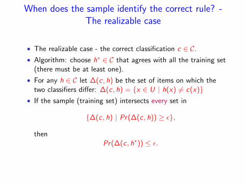
When does the sample identify the correct rule? -The realizable case
• The realizable case - the correct classification c ∈ C.
• Algorithm: choose h∗ ∈ C that agrees with all the training set(there must be at least one).
• For any h ∈ C let ∆(c , h) be the set of items on which thetwo classifiers differ: ∆(c, h) = {x ∈ U | h(x) 6= c(x)}
• If the sample (training set) intersects every set in
{∆(c , h) | Pr(∆(c , h)) ≥ ε},
thenPr(∆(c , h∗)) ≤ ε.

LearningaBinaryClassifier• Redandblueitems,possibleclassifica9onrules,andthesampleitems

When does the sample identify the correct rule?The unrealizable (agnostic) case
• The unrealizable case - c may not be in C.
• For any h ∈ C, let ∆(c, h) be the set of items on which thetwo classifiers differ: ∆(c, h) = {x ∈ U | h(x) 6= c(x)}
• For the training set {(xi , c(xi )) | i = 1, . . . ,m}, let
P̃r(∆(c , h)) =1
m
m∑i=1
1h(xi )6=c(xi )
• Algorithm: choose h∗ = arg minh∈C P̃r(∆(c , h)).
• If for every set ∆(c , h),
|Pr(∆(c, h))− P̃r(∆(c , h))| ≤ ε,
thenPr(∆(c , h∗)) ≤ opt(C) + 2ε.
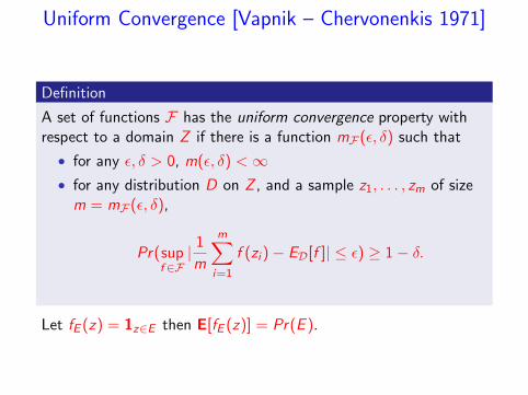
Uniform Convergence [Vapnik – Chervonenkis 1971]
Definition
A set of functions F has the uniform convergence property withrespect to a domain Z if there is a function mF (ε, δ) such that
• for any ε, δ > 0, m(ε, δ) <∞• for any distribution D on Z , and a sample z1, . . . , zm of size
m = mF (ε, δ),
Pr(supf ∈F| 1m
m∑i=1
f (zi )− ED[f ]| ≤ ε) ≥ 1− δ.
Let fE (z) = 1z∈E then E[fE (z)] = Pr(E ).

Uniform Convergence and Learning
Definition
A set of functions F has the uniform convergence property withrespect to a domain Z if there is a function mF (ε, δ) such that
• for any ε, δ > 0, m(ε, δ) <∞• for any distribution D on Z , and a sample z1, . . . , zm of size
m = mF (ε, δ),
Pr(supf ∈F| 1m
m∑i=1
f (zi )− ED[f ]| ≤ ε) ≥ 1− δ.
• Let FH = {fh | h ∈ H}, where fh is the loss function forhypothesis h.
• FH has the uniform convergence property ⇒ an ERM(Empirical Risk Minimization) algorithm ”learns” H.
• The sample complexity of learning H is bounded by mFH(ε, δ)

Uniform Convergence - 1971, PAC Learning - 1984
Definition
A set of functions F has the uniform convergence property withrespect to a domain Z if there is a function mF (ε, δ) such that
• for any ε, δ > 0, m(ε, δ) <∞• for any distribution D on Z , and a sample z1, . . . , zm of size
m = mF (ε, δ),
Pr(supf ∈F| 1m
m∑i=1
f (zi )− ED[f ]| ≤ ε) ≥ 1− δ.
• Let FH = {fh | h ∈ H}, where fh is the loss function forhypothesis h.
• FH has the uniform convergence property ⇒ an ERM(Empirical Risk Minimization) algorithm ”learns” H. PACefficiently learnable if there a polynomial timeε, δ-approximation for minimum ERM.
• The sample complexity of learning H is bounded by mFH(ε, δ)

Uniform Convergence
Definition
A set of functions F has the uniform convergence property withrespect to a domain Z if there is a function mF (ε, δ) such that
• for any ε, δ > 0, m(ε, δ) <∞• for any distribution D on Z , and a sample z1, . . . , zm of size
m = mF (ε, δ),
Pr(supf ∈F| 1m
m∑i=1
f (zi )− ED[f ]| ≤ ε) ≥ 1− δ.
VC-dimension and Rademacher complexity are the two majortechniques to
• prove that a set of functions F has the uniform convergenceproperty
• charaterize the function mF (ε, δ)

Some Background
• Let z1, . . . , zm i.i.d. observation from distribution F (x), andFm(x) = 1
m
∑mi=1 1zi≤x (empirical distribution function)
• Strong Law of Large Numbers: for a given x ,
Fm(x)→a.s F (x) = Pr(z ≤ x).
• Glivenko-Cantelli Theorem (uniform convergence of{F (x) | x ∈ R}):
supx∈R|Fm(x)− F (x)| →a.s 0.
• Dvoretzky-Keifer-Wolfowitz Inequality (Kolmogorov-Smirnovditribution)
Pr(supx∈R|Fm(x)− F (x)| ≥ ε) ≤ 2e−2mε
2.
• VC-dimension characterizes uniform convergence property forarbitrary sets of events.

Simplest Uniform Convergence - Union Bound
Theorem
In the realizable case, any concept class C can be learned withm = 1
ε (ln |C|+ ln 1δ ) samples.
Proof.
We need a sample that intersects every set in the family of sets
{∆(c , c ′) | Pr(∆(c , c ′)) ≥ ε}.
There are at most |C| such sets, and the probability that a sampleis chosen inside a set is ≥ ε.The probability that m random samples did not intersect with atleast one of the sets is bounded by
|C|(1− ε)m ≤ |C|e−εm ≤ |C|e−(ln |C|+ln 1δ) ≤ δ.

How Good is This Bound? - Learning an Interval
• A distribution D is defined on universe that is an interval[A,B].
• The true classification rule is defined by a sub-interval[a, b] ⊆ [A,B].
• The concept class C is the collection of all intervals,
C = {[c , d ] | [c , d ] ⊆ [A,B]}
Theorem
There is a learning algorithm that given a sample from D of sizem = 2
ε ln 2δ , with probability 1− δ, returns a classification rule
(interval) [x , y ] that is correct with probability 1− ε.
Note that the sample size is independent of the size of the conceptclass |C|, which is infinite.

Learning an Interval
• If the classifica2on error is ≥ ε then the sample missed at least one of the the intervals [a,a’] or [b’,b] each of probability ≥ ε/2
A B a b
x y
ε/2 a’
Each sample excludes many possible intervals. The union bound sums over overlapping hypothesis. Need beIer characteriza2on of concept's complexity!
ε/2 b’

Proof.
Algorithm: Choose the smallest interval [x , y ] that includes all the”In” sample points.
• Clearly a ≤ x < y ≤ b, and the algorithm can only err inclassifying ”In” points as ”Out” points.
• Fix a < a′ and b′ < b such that Pr([a, a′]) = ε/2 andPr([b, b′]) = ε/2.
• If the probability of error when using the classification [x , y ] is≥ ε then either a′ ≤ x or y ≤ b′ or both.
• The probability that the sample of size m = 2ε ln 2
δ did notintersect with one of these intervals is bounded by
2(1− ε
2)m ≤ e−
εm2+ln 2 ≤ δ

• The union bound is far too loose for our applications. It sumsover overlapping hypothesis.
• Each sample excludes many possible intervals.
• Need better characterization of concept’s complexity!