1

3 CT Parameters that Influence the Radiation DoseHans Dieter Nagel, PhDPhilips Medical Systems, Science and Technology, Roentgenstr. 24, D-22335 Hamburg, Germanyhans-dieter.nagel@philips.com

The radiation exposure to patients undergoing CT exam-inations is determined by two factors: equipment-relatedfactors, i.e. the design of the scanner with respect to doseefficiency, and application-related factors, i.e. the way inwhich the radiologist or the radiographer makes use of

3.1 CT Dose Descriptors

The dose quantities used in projection radiography are notapplicable to CT for three reasons:

• First, the dose distribution inside the patient is com-pletely different from that for a conventional radiogram,where the dose decreases continuously from the entranceof the X-ray beam to its exit, with a ratio of between100 and 1000 to 1. In the case of CT, as a consequenceof the scanning procedure that equally irradiates thepatient from all directions, the dose is almost equallydistributed in the scanning plane. A dose comparison ofCT with conventional projection radiography in termsof skin dose therefore doesn’t make any sense.

• Second, the scanning procedure using narrow beamsalong the longitudinal z-axis of the patient implies thata significant portion of the radiation energy is depositedoutside the nominal beam width. This is mainly due topenumbra effects and scattered radiation produced inside

the beam.• Third, the situation in CT is further complicated by the

circumstances in which - unlike in conventional projec-tion radiography - the volume to be imaged is not irradi-ated simultaneously. This often leads to confusion aboutwhat the dose from a complete series of e.g. 15 slicesmight be compared with the dose from a single slice.

As a consequence, dedicated dose quantities that accountfor these peculiarities are needed: The ‘Computed Tomo-graphy Dose Index (CTDI)’, which is a measure of thelocal dose, and the ‘Dose-Length Product (DLP)’, repre-senting the integral radiation exposure associated with aCT examination. Fortunately, a bridge exists that enablesto compare CT with radiation exposure from other mo-dalities and sources; this can be achieved by the effectivedose (E). So there are three dose descriptors in all, whicheveryone dealing with CT should be familiar with.

3.1.1 Computed Tomography Dose Index

The ‘Computed Tomography Dose Index (CTDI)’ is thefundamental CT dose descriptor. By making use of thisquantity, the first two peculiarities of CT scanning are takeninto account: The CTDI (unit: Milligray (mGy)) is derivedfrom the dose distribution along a line which is parallel tothe axis of rotation for the scanner (= z-axis) and which isrecorded for a single rotation of the x-ray source. Fig. 3.1illustrates the meaning of this term: CTDI is the equivalentof the dose value inside the irradiated slice (beam) thatwould result if the absorbed radiation dose profile wereentirely concentrated to a rectangular profile of width equalto the nominal beam width N·h

col, with N being the number

of independent (i.e. non-overlapping) slices that are acquir-ed simultaneously. Accordingly, all dose contributionsfrom outside the nominal beam width, i.e. the areas underthe tails of the dose profile, are added to the area insidethe slice.

the scanner. In this chapter, the features and parametersinfluencing patient dose are outlined. First, however, a briefintroduction on the dose descriptors applicable to CT isgiven.

0

0.5

1

1.5

-5 -4 -3 -2 -1 0 1 2 3 4 5

Slice position [cm]

Rel

ativ

e d

ose

CTDI

N·hcol

Fig. 3.1 Illustration of the term ’Computed TomographyDose Index (CTDI)’: CTDI is the equivalent of the dosevalue inside the irradiated slice (beam) that would resultif the absorbed radiation dose profile were entirely concen-trated to a rectangular profile of width equal to the nomi-nal beam width N·h

col.

2 Chapter 3: CT Parameters that Influence the Radiation Dose

The corresponding mathematical definition of CTDItherefore describes the summation of all dose contributionsalong the z-axis:

CTDIN h

D(z) dzcol

( . )=⋅

⋅ ⋅−∞

+∞

∫13 1

where D(z) is the value of the dose at a given location, z,and N·h

col is the nominal value of the total collimation

(beam width) that is used for data acquisition. CTDI istherefore equal to the area of the dose profile (the ‘dose-profile integral’) divided by the nominal beam width. Inpractice, the dose profile is accumulated in a range of –50mm to + 50 mm relative to the centre of the beam, i.e.over a distance of 100 mm.

The relevancy of CTDI becomes obvious from the totaldose profile of a scan series with e.g. n=15 subsequentrotations (fig. 3.2). The average level of the total doseprofile, which is called ‘Multiple Scan Average Dose(MSAD)’ (Shope 1981), is higher than the peak value ofeach single dose profile. This increase results from thetails of the single dose profiles for a scan series. Obviously,MSAD and CTDI are exactly equal if the table feed TF isequal to the nominal beam width N·h

col, i.e. if the pitch

factor

pTF

N hcol

( . )=⋅

3 2

is equal to 1. In general (i.e. if the pitch is not equal to 1,see fig. 3.3), the relationship between CTDI and MSAD

is given byMSAD p CTDI ( . )= ⋅1 3 3

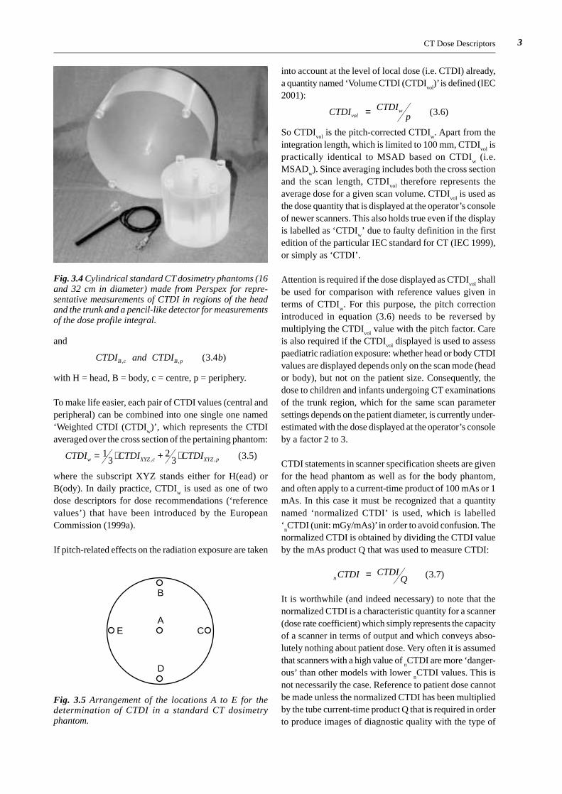
The practical implication of equation (3.3) is that - in orderto obtain the average dose for a scan series - it is notnecessary to carry out all the scans. Instead, it is sufficientto obtain the CTDI from a single scan by acquiring theentire dose profile according to equation (3.1). This isachieved with dose measurements using long, pencil-likedetectors, with an active length of 10 cm (fig. 3.4). Thesedetectors accumulate the dose profile integral (DPI, unit:mGy·cm), i.e. the area under the dose profile shown infig. 3.1. The CTDI is then obtained according to equation3.1 by division with the nominal beam width N·h

col.

In order to obtain estimates of the dose to organs that arelocated in the scan range, the CTDI generally refers tostandard dosimetry phantoms with patient-like diameters.In the standard measuring procedure for CTDI, whichutilizes two cylindrical Perspex (PMMA) phantoms ofdifferent diameter (fig. 3.4), dose is measured at the centreand near the periphery of the phantom (fig. 3.5). The largerphantom, being 32 cm in diameter, represents the absorp-tion that is typical for the trunk region of adults. Thesmaller phantom (16 cm in diameter) represents the patientin head examinations. The smaller phantom is also usedfor dose assessment in paediatric examinations (Shrimpton2000). The dose values thus obtained are denoted as

CTDI and CTDI aH c H p, , ( . )3 4

0

0.5

1

1.5

2

2.5

-10 -5 0 5 10

Slice position [cm]

Rel

ativ

e d

ose

MSAD

0

0.5

1

1.5

2

2.5

-10 -5 0 5 10

Slice position [cm]

Rel

ativ

e d

ose

MSAD

Fig. 3.2 Total dose profile of a scan series with n=15subsequent rotations. The average level of the total doseprofile, which is called ‘Multiple Scan Average Dose(MSAD)’, is equal to CTDI if the table feed TF is equalto the nominal beam width N·h

col (i.e. pitch p = 1).

Fig. 3.3 Total dose profile of a scan series with n=15subsequent rotations, scanned with pitch = 0.7,however. Due to the larger overlap, MSAD is higherthan in fig. 3.2 and amounts to CTDI divided by pitch.

3

and

CTDI and CTDI bB c B p, , ( . )3 4

with H = head, B = body, c = centre, p = periphery.

To make life easier, each pair of CTDI values (central andperipheral) can be combined into one single one named‘Weighted CTDI (CTDI

w)’, which represents the CTDI

averaged over the cross section of the pertaining phantom:

CTDI CTDI CTDIw XYZ c XYZ p= ⋅ + ⋅13

23 3 5, , ( . )

where the subscript XYZ stands either for H(ead) orB(ody). In daily practice, CTDI

w is used as one of two

dose descriptors for dose recommendations (‘referencevalues’) that have been introduced by the EuropeanCommission (1999a).

If pitch-related effects on the radiation exposure are taken

into account at the level of local dose (i.e. CTDI) already,a quantity named ‘Volume CTDI (CTDI

vol)’ is defined (IEC

2001):

CTDI CTDIpvol

w ( . )= 3 6

So CTDIvol

is the pitch-corrected CTDIw. Apart from the

integration length, which is limited to 100 mm, CTDIvol

ispractically identical to MSAD based on CTDI

w (i.e.

MSADw). Since averaging includes both the cross section

and the scan length, CTDIvol

therefore represents theaverage dose for a given scan volume. CTDI

vol is used as

the dose quantity that is displayed at the operator’s consoleof newer scanners. This also holds true even if the displayis labelled as ‘CTDI

w’ due to faulty definition in the first

edition of the particular IEC standard for CT (IEC 1999),or simply as ‘CTDI’.

Attention is required if the dose displayed as CTDIvol

shallbe used for comparison with reference values given interms of CTDI

w. For this purpose, the pitch correction

introduced in equation (3.6) needs to be reversed bymultiplying the CTDI

vol value with the pitch factor. Care

is also required if the CTDIvol

displayed is used to assesspaediatric radiation exposure: whether head or body CTDIvalues are displayed depends only on the scan mode (heador body), but not on the patient size. Consequently, thedose to children and infants undergoing CT examinationsof the trunk region, which for the same scan parametersettings depends on the patient diameter, is currently under-estimated with the dose displayed at the operator’s consoleby a factor 2 to 3.

CTDI statements in scanner specification sheets are givenfor the head phantom as well as for the body phantom,and often apply to a current-time product of 100 mAs or 1mAs. In this case it must be recognized that a quantitynamed ‘normalized CTDI’ is used, which is labelled‘

nCTDI (unit: mGy/mAs)’ in order to avoid confusion. The

normalized CTDI is obtained by dividing the CTDI valueby the mAs product Q that was used to measure CTDI:

n CTDI CTDIQ ( . )= 3 7

It is worthwhile (and indeed necessary) to note that thenormalized CTDI is a characteristic quantity for a scanner(dose rate coefficient) which simply represents the capacityof a scanner in terms of output and which conveys abso-lutely nothing about patient dose. Very often it is assumedthat scanners with a high value of

nCTDI are more ‘danger-

ous’ than other models with lower nCTDI values. This is

not necessarily the case. Reference to patient dose cannotbe made unless the normalized CTDI has been multipliedby the tube current-time product Q that is required in orderto produce images of diagnostic quality with the type of

CT Dose Descriptors

Fig. 3.4 Cylindrical standard CT dosimetry phantoms (16and 32 cm in diameter) made from Perspex for repre-sentative measurements of CTDI in regions of the headand the trunk and a pencil-like detector for measurementsof the dose profile integral.

AE

D

C

B

Fig. 3.5 Arrangement of the locations A to E for thedetermination of CTDI in a standard CT dosimetryphantom.

4 Chapter 3: CT Parameters that Influence the Radiation Dose

scanner under consideration. Only after having carried outthis step is it possible to decide if a particular scanner needsmore or less dose than another model for a specified typeof examination.

3.1.2 Dose-Length Product

The third peculiarity of CT, i.e. the question what the dosefrom a complete series of e.g. 15 slices might be comparedwith the dose from a single slice, is solved by introducinga dose descriptor named ‘dose-length product (DLP; unit:mGy·cm))’. DLP takes both the ‘intensity’ (representedby the CTDI

vol) and the extension (represented by the scan

length L) of an irradiation into account (fig. 3.6):

DLP CTDI Lvol ( . )= ⋅ 3 8

So the dose-length product increases with the number ofslices (correctly: with the length of the irradiated bodysection), while the dose (i.e. CTDI

vol) remains the same

regardless of the number of slices or length, respectively.In fig. 3.6, the area of the total dose profile of the scanseries represents the DLP. DLP is the equivalent of thedose-area product (DAP) in projection radiography, aquantity that also combines both aspects (intensity andextension) of patient exposure.

In sequential scanning, the scan length is determined bythe beam width N·h

col and the number n of tables feeds

TF:

L n TF N hcol ( . )= ⋅ + ⋅ 3 9

while in spiral scanning the scan length only depends onthe number n of rotations and the table feed TF:

L n TF Tt p N hrot

col ( . )= ⋅ = ⋅ ⋅ ⋅ 3 10

where T is the total scan time, trot

is the rotation time, andp is the pitch factor. While in sequential scanning the scanlength L is equal to the range from the begin of the firstslice till the end of the last, the (gross) scan length forspiral scanning not only comprises the (net) length of theimaged body section but also includes the additionalrotations at the begin and the end of the scan (‘over-ranging’) that are required for data interpolation.

If an examination consists of several sequential scan seriesor spiral scans, the dose-length product of the completeexamination (DLP

exam) is the sum of the dose-length pro-

ducts of each single series or spiral scan:

DLP DLPexam ii

( . )= ∑ 3 11

In daily practice, the DLP is used as the second (and mostimportant) of the two dose descriptors for dose recom-mendations (‘reference values’) that have been introduced

by the European Commission (1999a).

3.1.3 Effective Dose

CTDI and DLP are CT-specific dose descriptors that donot allow for comparisons with radiation exposures fromother sources, e.g. projection radiography, nuclearmedicine or natural background radiation. The onlycommon denominator to achieve this goal is the ‘EffectiveDose’. With effective dose, the organ doses from a partialirradiation of the body are converted into an equivalentuniform dose to the entire body.

Effective dose E (unit: Millisievert (mSv)) according toICRP 60 (ICRP 1991) is defined as the weighted averageof organ dose values H

T for a number of specified organs:

E w Hii

T i ( . ),= ⋅∑ 3 12

How much a particular organ contributes to effective dosedepends on its relative sensitivity for radiation-inducedeffects, as represented by the tissue-weighting factor w

i

attributed to the organ:

• 0.20 for gonads;• 0.12 for each of lungs, colon, red bone marrow and

stomach wall;• 0.05 for each of breast, urinary bladder, liver, thyroid

and oesophagus;• 0.01 for each of skeleton and skin;• 0.05 for the ‘remainder’

The ‘remainder’ consists of a group of additional organsand tissues with a lower sensitivity for radiation induced

Fig. 3.6 Total dose profile of a scan series with n=15 sub-sequent rotations. The dose-length product (DLP) is theproduct of the height (dose, i.e. CTDI

vol) and the width

(scan length L) of the total dose profile and is equal to thearea under the curve.

0

0.5

1

1.5

2

2.5

-10 -5 0 5 10

Slice position [cm]

Rel

ativ

e d

ose

Dose

Length L

5

effects for which the average dose must be used: smallintestine, brain, spleen, muscle tissue, adrenals, kidneys,pancreas, thymus and uterus. The sum of all tissue-weight-ing factors w

i is equal to 1.

Effective dose cannot as such be measured directly in vivo.Measurements in anthropomorphic phantoms with thermoluminescent dosemeters (TLD) are very time-consumingand therefore not well suited for daily practice. Effectivedose, however, can be assessed in various ways by usingconversion factors. For coarse estimates, it is sufficient tomultiply the dose-length product with mean conversionfactors, depending on which one out of three body regionswas scanned and whether the scan was made in head orbody scanning mode:

E DLP fmean ( . )≈ ⋅ 3 13

For adults of standard size, the following generic meanconversion factors f

mean apply:

• 0.025 mSv/mGy·cm for the head region• 0.060 mSv/mGy·cm for the neck region, scanned in head

mode• 0.100 mSv/mGy·cm for the neck region, scanned in body

mode• 0.175 mSv/mGy·cm for the trunk region

Similar factors (‘EDLP

’), which additionally distinguishbetween chest, abdomen and pelvis, but do not accountfor differences in scan mode, are given in report EUR16262 (European Commission 1999b).

In order to apply equation (3.13), the DLP or at least theCTDI

vol and the (gross) scan length L, from which the DLP

can be calculated according to equation (3.8), must be

Equipment-related Factors

available. If the scanner is not equipped with a dose display,or if a more detailed assessment of effective dose is desired(e.g. to be more specific for the scanned region of the body,to distinguish between males and females, to assess paedia-tric doses, or to take differences between scanners intoaccount), dedicated CT dose calculation software shouldbe used. These programs make use of more detailedconversion factors and also allow for calculation of organdoses. Currently, five different programs are either com-mercially available or in general use, which differ signific-antly in specifications, performance, and price. A compara-tive study on these programs has recently been publishedby Tack (2006).

Typical tolerances in effective dose assessment with theseprograms are in the order of ±20 to ±30%. Similar uncer-tainties also apply to effective dose assessment with TLDmeasurements in Alderson phantoms. This should alwaysbe born in mind when comparing doses from differentscanners in terms of effective dose. Care is also needed tonot mix up effective dose with organ doses, as both areexpressed in mSv. Nevertheless, effective dose is of greatvalue, e.g. to answer questions raised from patients. Forthis purpose, the annual natural background radiation,which is between 2 and 3 mSv in many countries, can beused as a scale.

A comprehensive compilation of dose-relevant scannerdata and other useful information required for CT doseassessment can be found in Nagel et al. (2002). The datagiven there apply to most of the scanners currently in useexcept for the most recent ones. However, data for thesenew scanners can be found in the CT-Expo software pack-age (Stamm and Nagel 2001) that is based on the data andformalism outlined in this book and is updated regularly.

3.2 Equipment-related Factors

3.2.1 Beam Filtration

In conventional projection radiography, beam filtration isa well-known means to reduce those portions of the radi-ation spectrum with no or little contribution to image for-mation. In the early years of CT history, beam filtrationwas comparatively large in order to compensate for beam-hardening artefacts. Filters made from 0.5 mm of copper,with filtering properties equivalent to approximately 18mm of aluminium (quality equivalent filtration, Nagel1986), were not unusual at that time. The present genera-tion of scanners typically employs a beam filtration forthe X-ray tube assembly of between 1 and 3 mm Al andan additional filtration (flat filter) of 0.1 mm Cu, giving atotal beam filtration of between 5 to 6 mm Al.

Apart from this, there are a number of older and also newerscanners which operate with an added filtration of appro-ximately 0.2 mm Cu, resulting in a total beam filtration ofbetween 8 and 9 mm Al, and sometimes even more (cur-rently up to 12 mm Al quality-equivalent filtration). Like-wise, there are also scanners that employ less filtration.Consequently, the normalised dose values for these scan-ners (

nCTDI in terms of mGy/mAs) differ significantly.

Very often these lower or higher values are misunderstoodas being an indicator that the equipment is more or lessdose-efficient compared with other scanners. This mightnot necessarily be the case in reality.

Apart from dose, the consequences on image qualityarising from the beam hardening and beam attenuating

6 Chapter 3: CT Parameters that Influence the Radiation Dose

properties of filtration have also to be considered (Nagel1989). The use of additional filtration impairs primarycontrast and increases noise due to reduced beam intensityper mAs as experienced by the detectors. Without compen-sating for these adverse effects (e.g. by increasing tubecurrent-time product), the contrast-to-noise ratio, whichaffects the detectability of small or low-contrast details, isreduced. Unpublished studies by the author show that, inorder to maintain the contrast-to-noise ratio (i.e. for con-stant image quality), the net reduction in terms of effectivedose achieved by increasing the standard beam filtration(1 mm Al + 0.1 mm Cu = 4.5 mm Al quality equivalent)by 0.2 mm Cu amounts to not more than 10%, even infavourable situations (soft tissue imaging, see fig. 3.7).Conversely, the same added filtration leads to higherpatient doses (up to 15%) in examinations with adminis-tration of contrast agents (iodine). At the same time, tubeloading must be increased by 20% in order to compensatefor reduced beam intensity.

Newer surveys on CT practice (e.g. Galanski et al. 2001)revealed that scanners of comparable age but with largelydiffering beam filtration are operated at almost similar doselevels. Similar results in terms of dose efficiency have beenfound in comparative tests on scanners with differing beamfiltration conducted by ImPACT (2004). Contrary to pro-jection radiography, which operates at comparatively lowertube potentials, beam filtration plays only a minor role inCT where higher tube potentials are applied. A return toincreased beam filtration - as sometimes recommendedor practised - is less advantageous than expected andshould only be made if sufficient X-ray tube loading

capacity is available or if other important aspects exist(e.g. improved performance of reconstruction filters).

3.2.2 Beam Shaper

Most scanners are equipped with a dedicated filter devicenamed ‘beam shaper’ or ‘bow-tie filter’ that modifies thespatial distribution of radiation emitted within the fanbeam. The purpose of this kind of filter (which is charac-terised by increasing thickness towards its outer edges) isto adapt the beam intensity to match the reduced attenua-tion of objects in the outer portions of the fan beam.

Rel

ativ

e do

se fr

ee-in

-air

z-axis

Beam width1·10 mm

a.

Nominal beam widthN·hcol = 4·5 mm

Slice collimation hcol dz

c.

Beam width2·5 mm

b.

Restrictivepost-patientcollimation

Detector array

Fig. 3.8 Dose profiles free-in-air with umbra (dark grey) and penumbra (light grey) portions for a single-slice scanner(a.), a dual-slice scanner (b.), and a quad-slice scanner (c.). With single- and dual-slice scanners, the width of theactive detector rows is sufficient to capture the entire dose profile, penumbra included (except for some scanners whichemploy restrictive post-patient collimation). For scanners with four and more slices acquired simultaneously, penumbrais excluded from detection in order to serve all detector channels equally well. The combined width of the penumbratriangles at both sides is characterized by the overbeaming parameter dz.

-20%

-10%

0%

10%

20%

Soft tissue Bone Iodine

Type of detail

Child

Adult

Ch

ang

es in

pat

ien

t d

ose

Fig. 3.7 Changes in patient dose due to increased beamfiltration at constant contrast-to-noise ration for differenttypes of detail. Standard filtration: 1 mm Al + 0.1 mm Cu(= 4.5 mm Al quality equivalent); added filtration: 0.2mm Cu (= 7 mm Al quality equivalent).

7

Dynamic range requirements for the detector system canthus be reduced. Simultaneously, beam-hardening effectsare also less likely.

In order to provide attenuating properties that are almosttissue equivalent, beam shapers should be made frommaterials containing only elements with a low atomicnumber Z. However, this is not always the case in practice.Beam shapers preferentially affect the dose in the outerportions of an object, thereby reducing the peripheralCTDI

p values. But as the dose at the centre is mainly caused

by scattered radiation from the periphery of the object,the central CTDI

c value is also somewhat reduced. The

ratio of dose at the periphery to the dose at the centretherefore decreases, making the dose distribution insidean object more homogeneous and so improving the unifor-mity of noise in the image. Contrary to the flat filter, thebeam shaper has a much greater impact on the dose proper-ties of a scanner.

The beam shapers found in practice not only differ by thematerial from which they are made. They also differ bytheir shape, thus producing more or less compensation. Aprominent example is the beam shaper of the Elscint CTTwin that was modified in 1998 to produce more compen-sation. In addition, different types of beam shapers can beselected on some scanners, depending on the nature anddiameter of the object (e.g. for head and body scanningmode).

3.2.3 Beam Collimation

The beam collimation for defining the thickness of theslice to be imaged is made in the first instance close to the

X-ray source (primary collimation). The shape of the doseprofile is determined by the aperture of the collimator, itsdistance from the focal spot, and the size and shape (i.e.the intensity distribution) of the focal spot. Due to thenarrow width of collimation, penumbral effects occur.These effects become more and more pronounced as colli-mation is further narrowed.

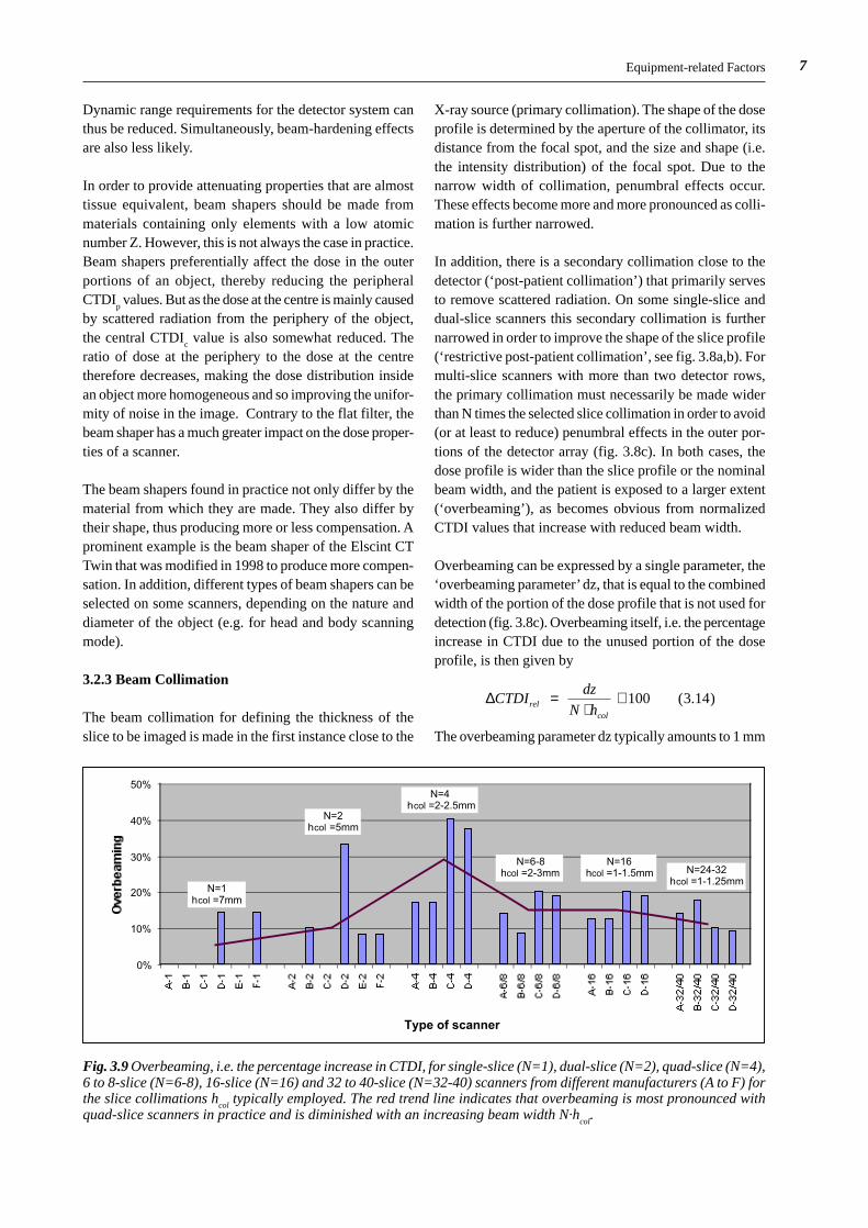
In addition, there is a secondary collimation close to thedetector (‘post-patient collimation’) that primarily servesto remove scattered radiation. On some single-slice anddual-slice scanners this secondary collimation is furthernarrowed in order to improve the shape of the slice profile(‘restrictive post-patient collimation’, see fig. 3.8a,b). Formulti-slice scanners with more than two detector rows,the primary collimation must necessarily be made widerthan N times the selected slice collimation in order to avoid(or at least to reduce) penumbral effects in the outer por-tions of the detector array (fig. 3.8c). In both cases, thedose profile is wider than the slice profile or the nominalbeam width, and the patient is exposed to a larger extent(‘overbeaming’), as becomes obvious from normalizedCTDI values that increase with reduced beam width.

Overbeaming can be expressed by a single parameter, the‘overbeaming parameter’ dz, that is equal to the combinedwidth of the portion of the dose profile that is not used fordetection (fig. 3.8c). Overbeaming itself, i.e. the percentageincrease in CTDI due to the unused portion of the doseprofile, is then given by

∆CTDIdz

N hrelcol

( . )=⋅

⋅ 100 3 14

The overbeaming parameter dz typically amounts to 1 mm

Equipment-related Factors

0%

10%

20%

30%

40%

50%

Type of scanner

N=1hcol =7mm

N=2hcol =5mm

N=4 hcol =2-2.5mm

N=6-8hcol =2-3mm

N=16hcol =1-1.5mm N=24-32

hcol =1-1.25mm

Fig. 3.9 Overbeaming, i.e. the percentage increase in CTDI, for single-slice (N=1), dual-slice (N=2), quad-slice (N=4),6 to 8-slice (N=6-8), 16-slice (N=16) and 32 to 40-slice (N=32-40) scanners from different manufacturers (A to F) forthe slice collimations h

col typically employed. The red trend line indicates that overbeaming is most pronounced with

quad-slice scanners in practice and is diminished with an increasing beam width N·hcol

.

8 Chapter 3: CT Parameters that Influence the Radiation Dose

for single- and dual-slice scanners that employ restrictivepost-patient collimation, and to 3 mm for multi-slice scan-ners with N = 4 and more slices that are acquired simulta-neously, but may vary depending on the type of scanner.For narrow beam width settings the increase in dose thatresults from overbeaming can be 100% and more.

In practice, overbeaming is no real issue for single- anddual-slice scanners, as the limited coverage restricts theuse of narrow beam width to a few examinations with ashort scan range (e.g. inner ear). With multi-slice scanners,however, overbeaming effects have to be taken seriously,as MSCT technology aims to provide improved resolutionalong the z-axis, which requires reduced slice collimation.Overbeaming, i.e. the increase in CTDI that results frombeam width settings that are typical for each type of scanneris shown in fig. 3.9 for a number of scanners from diffe-rent manufacturers. As indicated by the trend line, over-beaming is most pronounced with quad-slice scanners andis diminished with an increasing beam width N·h

col provid-

ed by scanners with more slices (Nagel 2005).

3.2.4 Detector Array

In contrast to single-slice scanners, multi-slice scannersare equipped with a detector array that consists of morethan a single row of detectors. Gas detectors or fourth-generation stationary detector rings are no longer compa-tible with multi-slice requirements. Consequently, onlythird-generation detector arcs with solid-state detectorshave remained. In general, solid-state detectors are moredose-efficient than gas detectors (van der Haar et al. 1998),but require additional means to suppress scattered radiation(anti-scatter-grids) that inevitably cause a certain loss ofprimary radiation, too.

The single detectors in a multi-row, solid-state detectorarray are separated by narrow strips (‘septa’) which arenot sensitive to radiation and therefore do not contributeto detector signal. Due to the large number of additional

strips, these inactive zones result in minor or major geome-trical losses, depending on the design of the detector array.In addition, further losses occur due to a decrease insensitivity at the edges of each row that results from cuttingthe scintillator crystal. In contrast to a single-row detectorarray whose width can be larger than the maximum slicethickness (see fig. 3.10), the edges of the rows in a multi-row detector array are located inside the beam. Due toboth these effects - separating strips and decreased sensi-tivity - the net efficiency of a solid-state detector array,which is typically 85% for single-slice scanners, is fur-ther decreased to typically 70%.

When 4-slice scanners were introduced in 1998, very dif-ferent detector designs were used (fig. 3.11), with varia-tions in the number of rows (between 8 and 34) and thesmallest detector size (between 0.5 and 1.25 mm). Thelarge number of rows (much larger than the number N ofslices that can be acquired simultaneously) was necessaryto enable the use of different slice collimations (between4·0.5 mm and 4·8 mm). Slice collimations wider than thedetector size are achieved by electronically combiningseveral adjacent detector rows (e.g. 4·1.25 mm = 5 mm

Single-slicescanner (N=1)

Multi-slicescanner (N=4)

Fig. 3.10 MSCT scanner, with simultaneous scanning offour slices, compared with a conventional single-slicescanner. Due to the additional septa between the detectorrows, the geometric efficiency of MSCT detector arraysis comparatively lower by 10 to 20%.

General Electric (LightSpeed QX/i, matrix)

16 · 1.25 mm

Toshiba (Aquilion Multi, hybrid)

4 · 0.5 mm 15 · 1 mm15 · 1 mm

Philips / Siemens (Mx8000 / Volume Zoom, progressive)

1 11.52.55 1.5 2.5 5 mm

Fig. 3.11 Detector arran-gement of four-slice scan-ners with significant dif-ferences in design (num-ber of rows, detector size,array width). Most ofthem are optimized for si-multaneous acquisition offour slices.

9Equipment-related Factors

(GE) or 1+1.5+2.5 = 5 mm (Philips/Siemens)). Eachdetector design had its specific advantages and drawbacks:Toshiba’s hybrid arrangement offered the largest coverage(32 mm) and the acquisition of four sub-millimetre slices,but had the largest number of septa (1 per mm) and thesmallest detector size (0.5 mm). The progressive design,commonly used by Philips and Siemens, had the smallestnumber of septa (0.35 per mm), but was restricted to twosub-millimetre slices only. GE’s matrix arrangement wasa compromise (0.75 per mm) that, however, facilitated thenext technology step towards eight simultaneously acquir-ed slices with the same detector array.

All 16-slice scanners introduced in 2001 now made use ofthe same hybrid design, with 16 smaller central detectors,accompanied by a number of larger detectors at both sides(fig. 3.12). Apart from the number of detector rows (bet-ween 24 and 40) and array width (between 20 and 32 mm),there were differences in the size of the detectors (between0.5 and 1.5 mm), and each manufacturer claimed his solu-tion to be the best one. As in real life, there are a numberof conflicting needs (spatial resolution, dose efficiency,coverage) that must be met, especially with respect to car-diac imaging where scan times below 20 s (one breathhold)

are mandatory. Consequently, designs, which put emphasisto a single one of these criteria, only were definitely notthe best compromise. Due to the increased number of septa(from 0.6 per mm (4-slice) to 1.1 per mm (16-slice) onaverage), the geometric efficiency of 16-slice detector ar-rays is somewhat lower.

In the latest generation of 64-slice scanners, matrix arran-gements that allow for simultaneous acquisition of 64 sub-millimetre slices are employed by the majority of manufac-turers (fig. 3.13). By electronically combining several ad-jacent rows, thicker slices can be acquired, too, but at areduced number of slices (e.g. 32·1.25 mm, 16·2.5 mmetc.). Once again, the number of septa was increased (to1.6 per mm on average), resulting in an additional loss ingeometric efficiency.

The hybrid detector design exclusively used by Siemensfor its Sensation 64 scanner is particular insofar as thenumber of simultaneous slices claimed by the manufac-turer (64) is much larger than the number of rows (32·0.6mm or 24·1.2 mm). The claim is based on a special acquisi-tion mode that employs two alternating focal spot positionsto simultaneously produce 64 data sets per rotation with

General Electric (LightSpeed 16)

16 · 0.625 mm 4 · 1.25 mm4 · 1.25 mm

Philips (Brilliance 16) / Siemens (Sensation 16)

16 · 0.75 mm 4 · 1.5 mm4 · 1.5 mm

Toshiba (Aquilion 16)

16 · 0.5 mm 12 · 1 mm12 · 1 mm

Fig. 3.12 Detector arran-gement of 16-slice scan-ners, all of them employ-ing a hybrid design, butwith differences in thenumber of rows, detectorsize, and array width.

Siemens (Sensation 64)

4 · 1.2 mm 32 · 0.6 mm 4 · 1.2 mm

General Electric (LightSpeed VCT)

64 · 0.625 mm

Philips (Brilliance 64)

64 · 0.625 mm

Toshiba (Aquilion 64)

64 · 0.5 mm

Fig. 3.13 Detector arran-gement of 64-slice scan-ners, most of them em-ploying a matrix designwith 64 rows of uniformsize. The Siemens designrefers to a 32-slice scan-ner that makes use of aparticular acquisitionmode (alternating focalspot) with 64 overlapping(i.e. non-independent)slices.

10 Chapter 3: CT Parameters that Influence the Radiation Dose

50% overlap in order to achieve a somewhat improvedspatial resolution in z-direction. With respect to all otherimportant features (collimation, coverage, overbeamingeffects etc.), however, this model behaves as a 32-slicescanner in submillimetre mode and a 24-slice scanner inall other modes at maximum. In addition, the thickness ofthe smallest slice that can be reconstructed (relevant forpartial volume effects) is at least equal to the smallest slicecollimation, i.e. 0.6 mm (Flohr et al. 2004), not lower.

3.2.5 Data Acquisition System

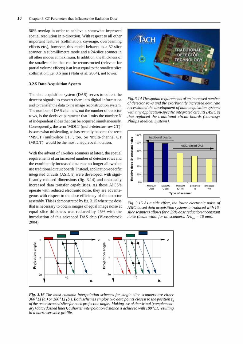
The data acquisition system (DAS) serves to collect thedetector signals, to convert them into digital informationand to transfer the data to the image reconstruction system.The number of DAS channels, not the number of detectorrows, is the decisive parameter that limits the number Nof independent slices that can be acquired simultaneously.Consequently, the term ‘MDCT (multi-detector-row CT)’is somewhat misleading, as has recently become the term‘MSCT (multi-slice CT)’, too. So ‘multi-channel CT(MCCT)’ would be the most unequivocal notation.

With the advent of 16-slice scanners at latest, the spatialrequirements of an increased number of detector rows andthe exorbitantly increased data rate no longer allowed touse traditional circuit boards. Instead, application-specificintegrated circuits (ASIC’s) were developed, with signi-ficantly reduced dimensions (fig. 3.14) and drasticallyincreased data transfer capabilities. As these AICS’soperate with reduced electronic noise, they are advanta-geous with respect to the dose efficiency of the detectorassembly. This is demonstrated by fig. 3.15 where the dosethat is necessary to obtain images of equal image noise atequal slice thickness was reduced by 25% with theintroduction of this advanced DAS chip (Vlassenbroek2004).

Fig. 3.14 The spatial requirements of an increased numberof detector rows and the exorbitantly increased data ratenecessitated the development of data acquisition systemswith tiny application-specific integrated circuits (ASIC’s)that replaced the traditional circuit boards (courtesy:Philips Medical Systems).

Fig. 3.15 As a side effect, the lower electronic noise ofASIC-based data acquisition systems introduced with 16-slice scanners allows for a 25% dose reduction at constantnoise (beam width for all scanners: N·h

col = 10 mm).

0

.

2.

z

z0

0

.

2.

z

z0a. b.

Pro

ject

ion

an

gle

Pro

ject

ion

an

gle

Fig. 3.16 The most common interpolation schemes for single-slice scanners are either360° LI (a.) or 180° LI (b.). Both schemes employ two data points closest to the position z

0of the reconstructed slice for each projection angle. Making use of the virtual (complement-ary) data (dashed lines), a shorter interpolation distance is achieved with 180° LI, resultingin a narrower slice profile.

0%

20%

40%

60%

80%

100%

120%

Mx8000Dual

Mx8000Quad

Mx8000IDT16

Brilliance16

Brilliance40

Type of scanner

ASIC-based DAS

traditional boards

Rel

ativ

e d

ose

@ c

on

stan

t n

ois

e

11Equipment-related Factors

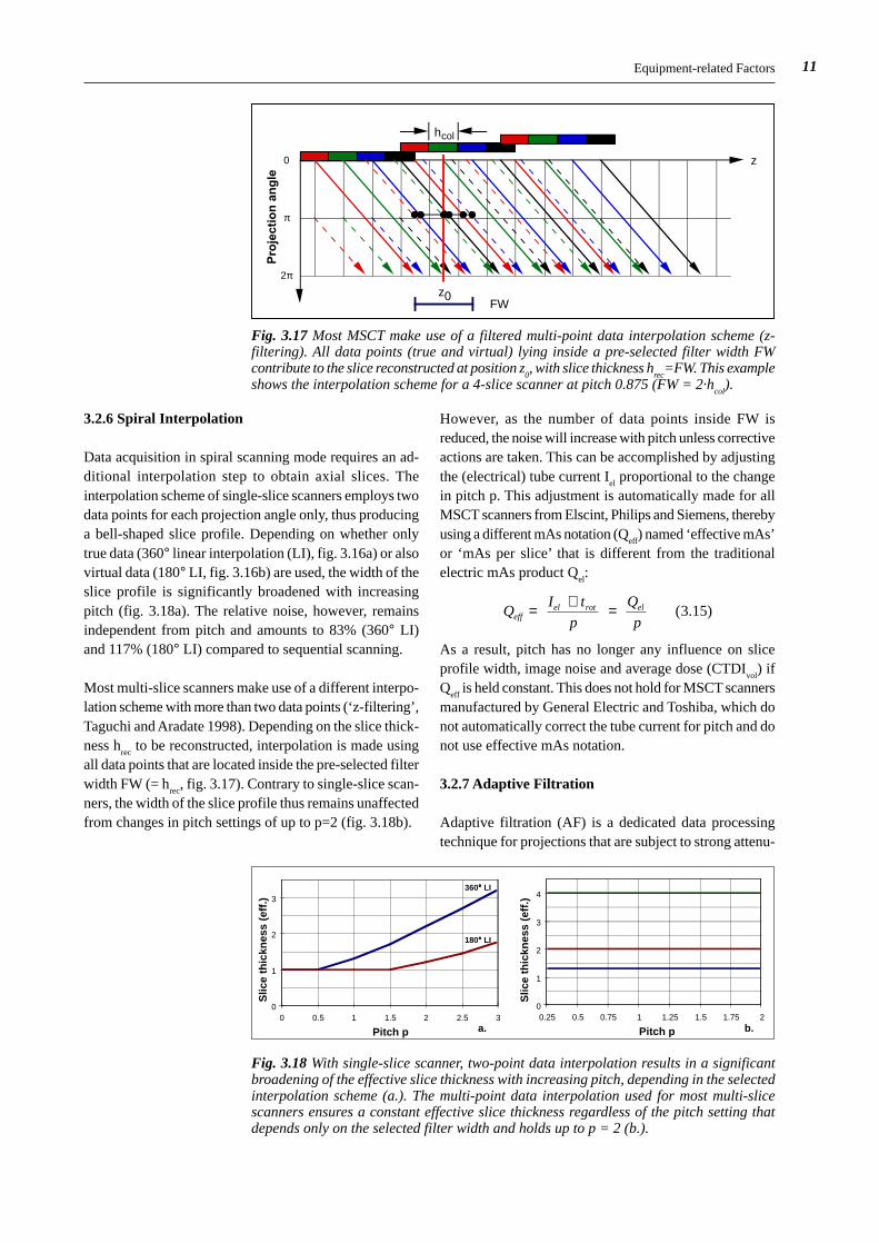
3.2.6 Spiral Interpolation

Data acquisition in spiral scanning mode requires an ad-ditional interpolation step to obtain axial slices. Theinterpolation scheme of single-slice scanners employs twodata points for each projection angle only, thus producinga bell-shaped slice profile. Depending on whether onlytrue data (360° linear interpolation (LI), fig. 3.16a) or alsovirtual data (180° LI, fig. 3.16b) are used, the width of theslice profile is significantly broadened with increasingpitch (fig. 3.18a). The relative noise, however, remainsindependent from pitch and amounts to 83% (360° LI)and 117% (180° LI) compared to sequential scanning.

Most multi-slice scanners make use of a different interpo-lation scheme with more than two data points (‘z-filtering’,Taguchi and Aradate 1998). Depending on the slice thick-ness h

rec to be reconstructed, interpolation is made using

all data points that are located inside the pre-selected filterwidth FW (= h

rec, fig. 3.17). Contrary to single-slice scan-

ners, the width of the slice profile thus remains unaffectedfrom changes in pitch settings of up to p=2 (fig. 3.18b).

However, as the number of data points inside FW isreduced, the noise will increase with pitch unless correctiveactions are taken. This can be accomplished by adjustingthe (electrical) tube current I

el proportional to the change

in pitch p. This adjustment is automatically made for allMSCT scanners from Elscint, Philips and Siemens, therebyusing a different mAs notation (Q

eff) named ‘effective mAs’

or ‘mAs per slice’ that is different from the traditionalelectric mAs product Q

el:

QI t

p

Q

peffel rot el= ⋅ =

( . )3 15

As a result, pitch has no longer any influence on sliceprofile width, image noise and average dose (CTDI

vol) if

Qeff

is held constant. This does not hold for MSCT scannersmanufactured by General Electric and Toshiba, which donot automatically correct the tube current for pitch and donot use effective mAs notation.

3.2.7 Adaptive Filtration

Adaptive filtration (AF) is a dedicated data processingtechnique for projections that are subject to strong attenu-

0

π

2π

z

hcol

z0FW

Pro

ject

ion

an

gle

Fig. 3.17 Most MSCT make use of a filtered multi-point data interpolation scheme (z-filtering). All data points (true and virtual) lying inside a pre-selected filter width FWcontribute to the slice reconstructed at position z

0, with slice thickness h

rec=FW. This example

shows the interpolation scheme for a 4-slice scanner at pitch 0.875 (FW = 2·hcol

).

0

1

2

3

0 0.5 1 1.5 2 2.5 3

Pitch p

Slic

e th

ickn

ess

(eff

.)

0

1

2

3

4

0.25 0.5 0.75 1 1.25 1.5 1.75 2

Pitch p

Slic

e th

ickn

ess

(eff

.)

a. b.

360°°°° LI

180°°°° LI

Fig. 3.18 With single-slice scanner, two-point data interpolation results in a significantbroadening of the effective slice thickness with increasing pitch, depending in the selectedinterpolation scheme (a.). The multi-point data interpolation used for most multi-slicescanners ensures a constant effective slice thickness regardless of the pitch setting thatdepends only on the selected filter width and holds up to p = 2 (b.).

12 Chapter 3: CT Parameters that Influence the Radiation Dose

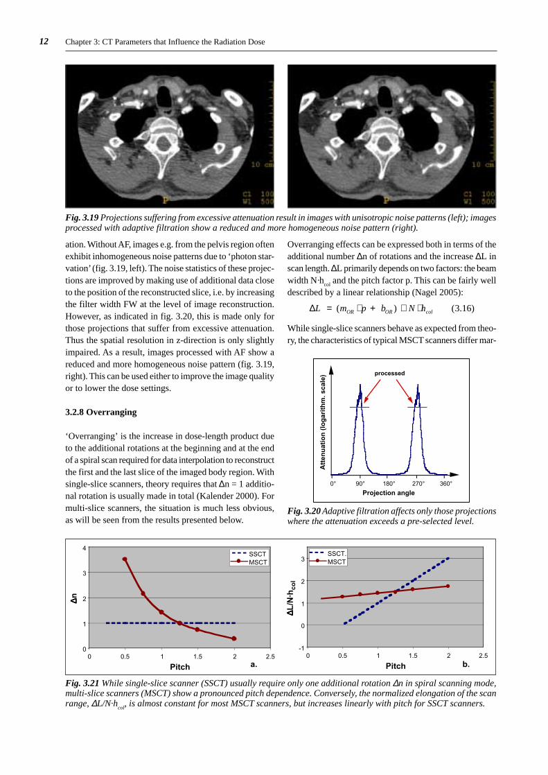
ation. Without AF, images e.g. from the pelvis region oftenexhibit inhomogeneous noise patterns due to ‘photon star-vation’ (fig. 3.19, left). The noise statistics of these projec-tions are improved by making use of additional data closeto the position of the reconstructed slice, i.e. by increasingthe filter width FW at the level of image reconstruction.However, as indicated in fig. 3.20, this is made only forthose projections that suffer from excessive attenuation.Thus the spatial resolution in z-direction is only slightlyimpaired. As a result, images processed with AF show areduced and more homogeneous noise pattern (fig. 3.19,right). This can be used either to improve the image qualityor to lower the dose settings.

3.2.8 Overranging

‘Overranging’ is the increase in dose-length product dueto the additional rotations at the beginning and at the endof a spiral scan required for data interpolation to reconstructthe first and the last slice of the imaged body region. Withsingle-slice scanners, theory requires that ∆n = 1 additio-nal rotation is usually made in total (Kalender 2000). Formulti-slice scanners, the situation is much less obvious,as will be seen from the results presented below.

Fig. 3.19 Projections suffering from excessive attenuation result in images with unisotropic noise patterns (left); imagesprocessed with adaptive filtration show a reduced and more homogeneous noise pattern (right).

Projection angle

Att

enu

atio

n (

log

arit

hm

. sca

le)

0° 90° 180° 270° 360°

processed

Fig. 3.20 Adaptive filtration affects only those projectionswhere the attenuation exceeds a pre-selected level.

Fig. 3.21 While single-slice scanner (SSCT) usually require only one additional rotation ∆n in spiral scanning mode,multi-slice scanners (MSCT) show a pronounced pitch dependence. Conversely, the normalized elongation of the scanrange, ∆L/N·h

col, is almost constant for most MSCT scanners, but increases linearly with pitch for SSCT scanners.

Overranging effects can be expressed both in terms of theadditional number ∆n of rotations and the increase ∆L inscan length. ∆L primarily depends on two factors: the beamwidth N·h

col and the pitch factor p. This can be fairly well

described by a linear relationship (Nagel 2005):

∆L m p b N hOR OR col ( ) ( . )= ⋅ + ⋅ ⋅ 3 16

While single-slice scanners behave as expected from theo-ry, the characteristics of typical MSCT scanners differ mar-

0

1

2

3

4

0 0.5 1 1.5 2 2.5

Pitch

SSCTMSCT

-1

0

1

2

3

0 0.5 1 1.5 2 2.5

Pitch

SSCT.MSCT

∆∆∆∆ n

∆∆∆∆ L/N

·hco

l

a. b.

13Equipment-related Factors

kedly. The number ∆n of additional rotations (fig. 3.21a)is strongly pitch dependent, while the normalized elonga-tion of the scan range, ∆L/N·h

col, is almost independent

from pitch (fig. 3.21b) and amounts to approximately 1.5,i.e. ∆L is typically 1.5 times the total beam width N · h

col.

For most single-slice scanners, the overranging parametersm

OR and b

OR are equal to 2 and –1, respectively. For the

majority of MSCT scanners, typical values for mOR

andb

OR are 1 and 0.5, respectively.

The implications of overranging effects for the radiationexposure to the patient, i.e. the dose-length product DLP,not only depend on ∆L, but also on the length L

net of the

imaged body region. The percentage increase in DLP isgiven by

∆ ∆DLP

L

Lrelnet

( . )= ⋅ 100 3 17

0%

10%

20%

30%

40%

50%

Type of scanner

N=1hcol =7mm

p=1.5

N=2hcol =5mm

p=1.5

N=4 hcol =2-2.5mm

p=1.5 N=6-8hcol =2-3mm

p=1

N=16hcol =1-1.5mm

p=1

N=24-32hcol =1-1.25mm

p=1

Ove

rran

gin

g @

L=

20cm

Fig. 3.22 Overranging, i.e. the percentage increase in DLP, for single-slice (N=1), dual-slice (N=2), quad-slice (N=4),6 to 8-slice (N=6-8), 16-slice (N=16) and 32 to 40-slice (N=32-40) scanners from different manufacturers (A to F) fora scan length L of 20 cm and the slice collimations and pitch settings typically employed. The red trend line indicatesthat overranging becomes more pronounced with scanners that allow for a wider beam width N·h

col.

and will be largest if ∆L is large and Lnet

is small.

The extent of overranging is shown in fig. 3.22 for arepresentative selection of single and multi-slice scannersfrom different manufacturers for typical scan parametersettings and a typical scan length of 20 cm. Overrangingeffects are normally almost negligible for single-slice andthe majority of dual- and quad-slice scanners. Contrary tooverbeaming, overranging becomes larger with an increas-ing number of slices acquired simultaneously due to theenlarged beam width. Even greater values might occurfor beam widths larger than the typical ones assumed hereand scan ranges being shorter than 20 cm.

3.2.9 Devices for Automatic Dose Control

Newer scanners are equipped with means that automa-tically adapt the mAs settings to the individual size and

Fig. 3.23 Automatic exposure control (AEC) accounts forthe average attenuation of the patient’s body region thatis to be scanned. For slim patients, mAs is reduced to alevel that ensures constant image quality.

100%

50%

z-axis

Standard mAs

Average mAs

Modulated mAs

Fig. 3.24 Longitudinal dose modulation (LDM) is arefinement of AEC that adapts the mAs settings slice-by-slice or rotation by rotation. Those parts of the scan rangewith reduced attenuation will be less exposed.

14 Chapter 3: CT Parameters that Influence the Radiation Dose

shape of the patient. As this matter is discussed in detailin chapter 6, only a brief overview shall be given here.

Automatic dose control systems offer up to four differentfunctionalities, which can be used either alone or incombination:

• Automatic exposure control (AEC, fig. 3.23) thataccounts for the average attenuation of the patient’s bodyregion that is to be scanned. Information on the patient’sattenuation properties is derived from the scan projectionradiogram (SPR) usually recorded prior to the scan forplanning purposes.

• Longitudinal dose modulation (LDM, fig. 3.24), whichis a refinement of AEC by adapting the mAs settingslocally, i.e. slice-by-slice or rotation by rotation.

• Angular dose modulation (ADM, fig. 3.25), anotherrefinement of AEC that adapts the tube current to thevarying attenuation at different projection angles. In-formation on the patient’s attenuation properties is eitherderived from two SPR or in real-time from the precedingrotation.

• Temporal dose modulation (TDM, fig. 3.26) that re-duces the tube current in cardiac CT (or other ECG-gated CT examinations) during those phases of thecardiac cycle that are not suited for image reconstruc-tion due to excessive object motion.

The common denominator of these functionalities is thatthe user no longer needs to select his parameter settings

A

B

Increasedattenuation

Reducedattenuation

100%

A B A B A

50%

Standard mAs

Average mAs

Modulated mAs

Projectionangle

0%

Fig. 3.25 Angular dosemodulation (ADM) is another refinement of AECthat adapts the tube cur-rent to the varying attenu-ation at different projec-tion angles. Those projec-tions with reduced attenu-ation will be less exposed.

20

40

60

80

100

Rel

ativ

e tu

be

curr

ent

(%)

0

Timen n+1 n+2 n+3

400 ms

250 ms

ECG signalTube current Data window

Fig. 3.26 In cardiac CT(or other ECG-gated CTexaminations), temporaldose modulation (TDM)reduces the tube currentduring those phases ofthe cardiac cycle that arenot suited for image re-construction due to ex-cessive object motion.

with respect to the ‘worst case’, i.e. obese patients, thepart of the scan range with the highest attenuation (e.g.shoulder in chest exams), the projection with the highestattenuation (lateral) etc.. Consequently, a significant dosereduction from the application of these devices can beexpected.

All major CT manufacturers now offer some or all of thesefunctionalities with their latest scanners. A comprehensivereport on the current status of automatic dose controlsystems has been published by ImPACT (2005). However,there are significant differences how these devices operateand perform. At present, some of these systems are notsufficiently user-friendly and make adjustments in a waythat seems to be theoretically sound, but does not complywith other, more comprehensive aspects of image quality.Some of these shortcomings will be discussed in thefollowing section.

3.2.10 Dose Display

Newer scanners must be equipped with a dose display. Atpresent, only the display of CTDI

vol is mandatory (IEC

2001). However, many scanners already show the DLP,too, either per scan series or both DLP per scan series andDLP per exam. An example with display of CTDI

vol and

DLP per scan series is shown in fig. 3.27.

With the dose display, dose is not saved per se, but feed-back is provided that may help to achieve this goal, e.g.

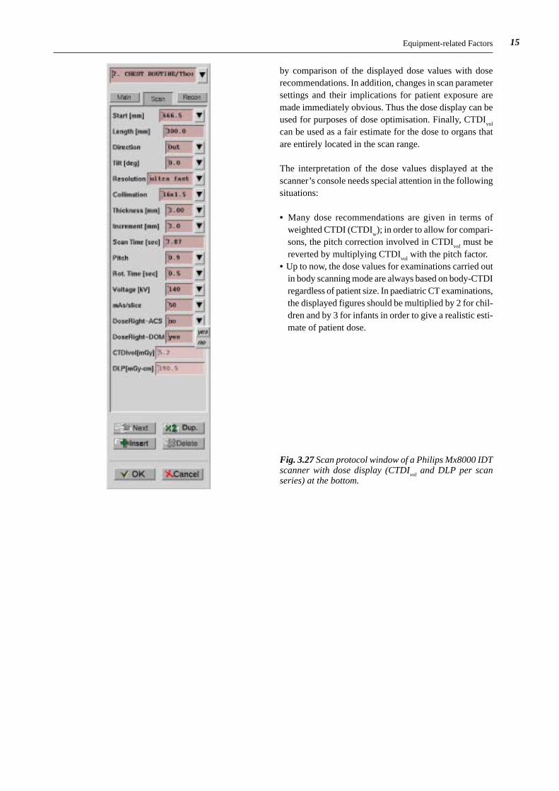
15

Fig. 3.27 Scan protocol window of a Philips Mx8000 IDTscanner with dose display (CTDI

vol and DLP per scan

series) at the bottom.

by comparison of the displayed dose values with doserecommendations. In addition, changes in scan parametersettings and their implications for patient exposure aremade immediately obvious. Thus the dose display can beused for purposes of dose optimisation. Finally, CTDI

vol

can be used as a fair estimate for the dose to organs thatare entirely located in the scan range.

The interpretation of the dose values displayed at thescanner’s console needs special attention in the followingsituations:

• Many dose recommendations are given in terms ofweighted CTDI (CTDI

w); in order to allow for compari-

sons, the pitch correction involved in CTDIvol

must bereverted by multiplying CTDI

vol with the pitch factor.

• Up to now, the dose values for examinations carried outin body scanning mode are always based on body-CTDIregardless of patient size. In paediatric CT examinations,the displayed figures should be multiplied by 2 for chil-dren and by 3 for infants in order to give a realistic esti-mate of patient dose.

Equipment-related Factors

16 Chapter 3: CT Parameters that Influence the Radiation Dose

Although the scanner design is of some importance, sur-veys on CT practice have regularly shown that the wayhow the scanner is used has the largest impact on the dosesapplied in a CT examination. The application-related fac-tors on which patient exposure depends are subdivided in

• scan parameters, i.e. those factors that directly determinethe local dose level (CTDI

vol) and that are often pre-

installed or recommended by the manufacturer (e.g. inapplication guides);

• examination parameter, i.e. those factors that – in combi-nation with CTDI

vol - determine the integral exposure

(i.e. DLP) and that depend on the preferences of theuser;

• reconstruction and viewing parameters, which implicitlyinfluence the dose settings.

First, however, the pricipal interdependences between dosesettings and image quality shall be outlined

3.3.1 Brooks’ Formula

As in conventional projection radiography, aspects of doseand image quality are linked. For CT, Brooks and DiChiro(1976) have formulated the correlation between these twoopposed quantities:

DB

a b hwith B d exp ( . )∝

⋅ ⋅ ⋅= − ⋅

σµ

2 2 3 18

where

D = patient doseB = attenuation factor of the objectµ = mean attenuation coefficient of the objectd = diameter of the objectσ = standard deviation of CT numbers (noise)a = sample incrementb = sample widthh = slice thickness

This fundamental equation - commonly known as the‘Brooks’ formula’ - describes what happens with respectto patient dose if one of the parameters is changed whileimage noise remains constant:

• dose must be doubled if slice thickness is cut by half;• dose must be doubled if object diameter increases by 4

cm;• an eightfold increase in dose is required if spatial resolu-

tion is doubled (by cutting sample width and sampleincrement by half).

3.3 Application-related Factors

In this context, the term ‘dose’ is applicable to each of thedose quantities that are appropriate for CT. Dose and noiseare inversely related to each other in such a way that afourfold increase in dose is required if noise is to be cutby half.

It should be noted, however, that the Brooks’ formula isincomplete in that image quality is only considered in termsof quantum noise and spatial resolution. Other importantinfluences, such as contrast, electronic noise or artefacts,are not taken into account and will therefore modifyoptimization strategies under particular circumstances.

3.3.2 Scan Parameters

3.3.2.1 TUBE CURRENT-TIME PRODUCT (Q)

As in conventional radiology, a linear relationship existsbetween the tube current-time product and dose; i.e. alldose quantities will change by the same amount as theapplied mAs. The mAs product Q for a single sequentialscan is obtained by multiplying the tube current I andexposure time t; in spiral scanning mode, Q is the productof the tube current I and rotation time t

rot. This should not

be mixed up with the total mAs product of the scan whichis the product of tube current I and (total) scan time T.

The consequences on image quality resulting from varia-tions in the tube current-time product are relatively sim-ple to understand. The only aspect of image quality soaffected is image noise, which is - as indicated in equation(3.18) - inversely proportional to the square root of dose(i.e. mAs).

The tube current-time product is often used as a surrogatefor the patient dose (i.e. CTDI). However, this is highlymisleading, as the normalized CTDI values and thus thedose that results for the same mAs setting can vary by upto a factor 6 between different scanners. So it makes abso-lutely no sense to communicate dose information or recom-mendations on the basis of mAs. Instead, only CTDI

vol

(and DLP) should be used for this purpose.

With the advent of multi-slice scanners, additional confu-sion arose due to the introduction of a different, pitch-corrected mAs notation (‘effective mAs’ or ‘mAs perslice’, see equation (3.15)) by Elscint, Philips and Sie-mens. As most multi-slice scanners make use of a multi-point spiral interpolation scheme as outlined in section3.2.6, effective mAs is the most appropriate notation forMSCT. Nevertheless, General Electric and Toshiba stillprefer the traditional electrical mAs notation which fur-

17

ther makes it difficult to compare mAs settings from dif-ferent scanners. This particularly holds for cardiac CTwhere very low pitch settings are used.

RecommendationThe settings for the tube current-time product should beadapted to the characteristics of the scanner, the size ofthe patient (see section 3.3.2.5), and the dose requirementsof each type of examination. Examinations with high inhe-rent contrast, such as for chest or skeleton, that are charac-terised by viewing with wide window settings, can regular-ly be conducted at significantly reduced mAs settings.

3.3.2.2 TUBE POTENTIAL (U)

When the tube potential is increased, both the tube outputand the penetrating power of the beam are improved, whileimage contrast is adversely affected. In conventional pro-jection radiography, increased tube potentials are applied

in order to ensure short exposure times for obese patients,to equalize large differences in object transmission (e.g.during chest examinations) or to reduce patient dose. Inthe latter case, automatic exposure control (AEC) guaran-tees that the improved penetrating power of the beam isexclusively for the benefit of the patient.

In CT, increased tube voltages are used preferentially forimprovements in tube loading and image quality. Contraryto the case for mAs, the consequences of variations in kVcannot easily be assessed. The relationship between doseand tube potential U is not linear, but rather of an exponen-tial nature which varies according to the specific circum-stances. The intensity of the radiation beam at the detectorarray, for example, varies with U to the power of 3.5. Ifthe tube potential is increased e.g. from 120 to 140 kV, theelectrical signal obtained from the detectors thereforechanges by a factor 1.7 (fig. 3.28).

The decrease in primary contrast which normally resultsfrom this action is largely over-compensated by the associ-ated decrease in noise, i.e. the higher the tube potential,the better the contrast-to-noise ratio CNR (except for theapplication of iodine as contrast agent). The only reasonwhy this analysis generally holds true is the absence ofany kind of AEC in the majority of scanners which mightprevent unnecessary increases in the detector signal. Thisclearly demonstrates that dose is not reduced by applyinghigher kV settings, but merely increased as long as mAssettings are not changed: weighted CTDI and effectivedose increase with U to the power of 2.5 (fig. 3.28), whichmeans that both are increased by approximately 50% ifkV settings are changed from 120 to 140 kV.

Therefore the question is justified whether and when itmight be reasonable to deviate from the 120 kV settingusually applied. As can be seen from fig. 3.29, this dependson the attenuation characteristics of the detail that isdiagnostically relevant. The figures are given in terms ofcontrast-to-noise ratio squared (CNR2) at constant patientdose; this notation allows to directly convert the percentagedifferences into dose differences. For soft tissue contrast(e.g.differences in tissue density), higher tube potentialsperform slightly better than lower ones, but the differencesare quite small. The opposite holds true for bone contrast(i.e. bone vs. tissue). For iodine contrast, however, thereis a strong dependence on tube potential that is much infavour of lower kV settings. So 80 instead of 120 kV wouldallow to reduce the patient dose by almost a factor of twowithout sacrifying image quality.

Application-related Factors

Fig. 3.28 Voltage dependence of patient dose (CTDIw) and

detector signal (reference: 120 kV).

0

25

50

75

100

125

150

175

200

Soft tissue Bone Iodine

Type of detail

80 kV

100 kV

120 kV

140 kV

CN

R2

@ c

on

stan

t d

ose

(a.

u.)

Fig. 3.29 Voltage dependence of contrast-to noise ratiosquared (CNR2) at constant patient dose (CTDI

w) for dif-

ferent types of detail. While CNR2 is almost constant forimaging of soft tissue and bone, imaging performance issignificantly improved for iodine at lower voltages.

0%

25%

50%

75%

100%

125%

150%

175%

200%

80 100 120 140

Tube potential U [kV]

Patient

Detector

Rel

ativ

e D

ose

18 Chapter 3: CT Parameters that Influence the Radiation Dose

RecommendationTube potentials other than 120 kV should be consideredonly in case of

• obese patients where mAs cannot further be increased:use higher kV settings

• slim patients and paediatric CT where mAs cannot fur-ther be reduced: use lower kV settings

• CT angiography with iodine: use lower kV settings.

Variations in tube potential should not be considered forpure dose reduction purposes except for CT angiography.Due to the complexity involved, adaptation of mAs settingsshould not be left to automatic exposure control systems,as these do not account for changes in contrast. Dosesettings in CT angiography should not be higher than inunenhanced scans of the same body section and should belowered if performed at reduced kV settings.

3.3.2.3 SLICE COLLIMATION (hcol

) AND SLICETHICKNESS (h

rec)

With single-slice CT, the slice collimation hcol

used fordata acquisition and the reconstructed slice thickness h

rec

used for viewing purposes were identical (except for sliceprofile broadening in spiral scans with increased pitch asdiscussed in section 3.2.6). So there was no need todistinguish between both of them. With multi-slice CT,the slice collimation (e.g. 0.75 mm) and the reconstructedslice thickness (e.g. 5 mm) are usually different. Frequent-ly, the selection of the reconstructed slice thickness is madewith respect to multiplanar reformating (MPR) purposes(e.g. 1 mm), thus creating a so-called ‘secondary raw dataset’, i.e. a stack of thin slices from which MPR slabs withlarger thickness (e.g. 5 mm) can be made for viewing pur-poses.

The ability to acquire longer body sections with thin slicesin order to achieve an almost isotropic spatial resolutionis the most important achievement of multi-slice technol-ogy. As reduced slice thickness is associated with increasedimage noise, this may have a significant impact on patientdose as expressed by the Brooks’ formula (equation 3.18).Therefore it is worth while to treat this matter in a some-what more detailed fashion.

A narrow slice collimation is a precondition for a narrowslice thickness, but its impact on patient dose is restrictedto aspects of overbeaming and overranging only. As theseshow opposed dependences on beam width, as outlined insections 3.2.3 and 3.2.8, the question arises for the opti-mized beam width settings. As demonstrated for a typicalMSCT scanner in fig. 3.30, beam width settings greaterthan 10 mm perform almost equally well (a.) except forshort scan ranges (spine, paediatrics) where a beam width

Fig. 3.30 Increased dose-length product due to overbeaming (OB) and overranging (OR) effects for a typical MSCTscanner. For avarage to long scan ranges (L = 20 cm and more, a.), all beam width settings above 10 mm performalmost equally well. For short scan ranges (L = 10 cm as in paediatric and spine exams, b.), beam width settingsbetween 10 and 20 mm should be preferred.

0%

20%

40%

60%

80%

100%

0 10 20 30 40

Beam width [mm]

OBOROB+OR

0%

20%

40%

60%

80%

100%

0 10 20 30 40

Beam width [mm]

Incr

ease

in D

LP

@ L

=20

cm

OBOROB+OR

a. b.

Incr

ease

in D

LP

@ L

=10

cm

0.1

1

10

0 2 4 6 8 10 12

Slice thickness hrec [mm]

Contrast

1/Noise

CNR

Rel

ativ

e im

age

qu

alit

y (a

.u.)

Fig. 3.31 Relative image quality in dependence of the sliceshickness h

rec. Improvements in image quality (better de-

tail contrast due to reduced partial volume effects) out-weigh the detoriations caused by increased noise. As aresult there is a net gain in contrast-to-noise ratio (CNR)at reduced slice thickness without any increase in dose.

19

of between 10 and 20 mm is more appropriate (b.). Beamwidth settings below 10 mm should be avoided due toincreased overbeaming effects unless there are other im-portant aspects that justify to override this recommend-ation.

The decisive determinant with respect to image noise andits implications for patient dose, however, is the slice thick-ness h

rec that is finally used for viewing purposes. The rela-

tionship between slice thickness, noise and dose expressed

in the Brooks’ formula tempts to correct any reduction inslice thickness by a corresponding increase in dose toensure a constant image noise, and some automaticexposure control systems exactly do so. However, anyvariation in slice thickness also affects image contrast dueto a modification in partial volume effect, which is nottaken into account by the Brooks’ formula. As shown infig. 3.31, image noise and image contrast of small detailswill react in a different fashion on reduction of the slicethickness: while image quality in terms of noise is impaired

Application-related Factors

Fig. 3.32 MSCT examination of the liver performed on a MSCT scanner (Siemens Somatom Volume Zoom) at 120 kV,4·2.5 mm slice collimation and 125 mAs

eff (CTDI

vol = 11 mGy). From the same raw data set, slices of different thickness

(3 mm (a.), 5 mm (b.), 7 mm (c.), and 10 mm (d.)) were reconstructed at the same central position z0. Despite the

increased noise pertaining for thinner slices, the visibility of small lesions improves remarkably owing to reducedpartial volume effects. This is clearly demonstrated by a lesion approximately 3 mm in size (arrow) (courtesy Dr.Wedegaertner, University Hospital Eppendorf, Hamburg, Germany).

c .c .c .c .c . d .d .d .d .d .

a .a .a .a .a . b .b .b .b .b .

20 Chapter 3: CT Parameters that Influence the Radiation Dose

proportional to the square root of the change in slice thick-ness only, the contrast is improved proportional to the slicethickness. As a result, there is a net gain in image qualityin terms of contrast-to-noise ratio CNR without any inceasein dose whenever partial volume effect is of importance.

This is clearly demonstrated by the clinical example givenin fig. 3.32, where the visibility of a liver lesion (approxim-ately 3 mm in size) diminishes continually with increasingslice thickness – despite reduced image noise. In addition,a detailed analysis of the results of the German survey onCT practice in 1999 (Galanski et al. 2001) has revealedthat slice thickness has only minor or no influence on cli-nical dose settings. This is shown in fig. 3.33 for liverexaminations with slice thicknesses of between 3 and 10mm that were used in practice. Therefore it is essential tounderstand that the selection of a narrow slice collimationis only a means to an end: to enable MPR images withoutor with reduced step artefacts, and, if necessary, to over-come partial volume effects.

Recommendation:The slice collimation should be selected as small as com-patible with aspects of overbeaming/overranging, totalscan time and tube power. Viewing should preferentiallybe made with thicker slabs (e.g. 3 to 8 mm), therebyreducing image noise and other artefacts. Thinner slabsshould only be used if partial volume effect is of impor-tance. This should preferentially be done in conjunctionwith workstations that allow to change the slab thicknessin real-time. Except for very narrow slices there shouldbe no need for any increase in dose settings on reductionof slice thickness.

3.3.2.4 PITCH (p)

With SSCT scanners, scanning at increased pitch settings

primarily serves to increase the speed of data acquisition.As a side effect, patient dose is reduced accordingly, atthe expense of impaired slice profile width, i.e. z-resolu-tion, however. As already outlined in section 3.2.6, MSCTscanners make use of a spiral interpolation scheme that isdifferent from SSCT. Thus the slice profile width remainsunaffected from changes in pitch settings. Instead, imagenoise changes with pitch (fig. 3.34a) unless the tube currentis adapted accordingly.

Scanners that make use of the effective mAs (mAs perslice) concept not only keep slice profile width, but alsoimage noise constant when pitch changes (fig. 3.34a). Toachieve this goal, the electrical mAs product supplied tothe x-ray tube automatically changes linearly with pitch(fig. 3.34b). As a consequence, patient dose (CTDI

vol) is

no longer reduced at increased pitch settings in contrastto SSCT scanners. On the other hand, dose will also notincrease at reduced pitch settings. MSCT scanners withoutautomatic adaptation of mAs will still save dose at in-creased pitch setting, but this will happen at impaired

0

5

10

15

20

25

30

3 mm 5 mm 7 mm 8 mm 10 mm Average

Slice thickness

CT

DI w

[m

Gy]

Fig. 3.33 The patient dose (CTDIw) for liver examinations,

applied by the participants of the German CT survey 1999,was almost constant despite the selection of different slicethicknesses.

0

0.5

1

1.5

2

0.25 0.5 0.75 1 1.25 1.5 1.75 2

Pitch p

Rel

ativ

e n

ois

e (a

.u.)

electrical mAs = constant

effective mAs = constant

a.

0

0.5

1

1.5

2

2.5

0.25 0.5 0.75 1 1.25 1.5 1.75 2

Pitch p

Ele

ctri

cal m

As

pro

du

ct

SSCT, MSCT withouteffective mAs

MSCT with effective mAs

b.

Fig. 3.34 For MSCT systems that employ multi-point spiral data interpolation (z-filtering), image noise changes withpitch unless effective mAs is held constant (a.). This implies that the electrical mAs product supplied to the tubechanges with pitch (b.). Contrary to SSCT, changes in pitch settings therefore no longer have any influence on patientdose in terms of CTDI

vol.

21Application-related Factors

image quality (more noise) as long as mAs is not adaptedmanually.

Frequently, image quality in terms of artefacts dependson pitch settings. In general, spiral artefacts are reducedat lower pitch settings. For similar reasons, some scannersallow the setting of a limited number of ‘preferred’ pitchesonly. Reduced pitch settings can also be applied to enhancethe effective tube power, however, at the expense ofreduced scanning speed.

Recommendation:Pitch settings with MSCT scanners should be made exclu-sively with respect to scan speed, spiral artefacts and tubepower. Dose considerations no longer play a role if scan-ners that employ effective mAs are used or if (electrical)mAs is adapted to pitch to achieve constant image noise.

3.3.2.5 OBJECT DIAMETER (d)

Patient size, although not a parameter to be selected at thescanners’s console, represents an important influencingparameter that needs to be considered in this context.Considerable reductions in mAs settings are appropriatewhenever slim patients, and particularly children, areexamined. In order to avoid unnecessary over-exposure,the mAs must be intentionally adapted by the operatorunless AEC-like devices are available. Due to the decreas-ed attenuation for the smaller object, image quality willnot be impaired if mAs is selected appropriately. Thismeans that the image quality will be at least as good as forpatients of normal size, although the dose has beenreduced.

The two questions to be solved in this context are:

• To which degree shall mAs settings be adapted in depend-

ence of the object diameter d?• Which diameter is typical for a standard patient to whom

the standard protocol settings refer to?

From theoretical considerations (half-value thickness HVLfor CT beam qualities), mAs should be altered by a factor2 for each change in patient diameter of 4 cm tissue-equiv-alent thickness. However, dedicated studies (e.g. Wiltinget al. 2001) have shown that this algorithm doesn’t workwell in practice: Although objective (i.e. measured) noisewas almost constant for patient diameters of between 24and 36 cm, it was found that the subjective (i.e. perceived)image quality continually decreased with the patient dia-meter and vice versa. This is most likely due to the circum-stance that adipose patients have more fatty tissue aroundtheir organs. Thus the inherent contrast is better, and morenoise can be tolerated. The opposite holds true with slimpatients.

Consequently, a more gentle adaptation of mAs withpatient diameter (factor 2 in mAs per 8 cm change inpatient diameter) will better comply with clinical needs.Among the automatic exposure control systems currentlyin use, those from Philips and Siemens already make useof this modified algorithm that ensures a constant ‘ade-quate’ image quality, while those implemented by Gene-ral Electric and Toshiba simply attempt to ensure a constantnoise level. As already outlined in sections 3.3.2.2 for tubepotential and 3.3.2.3 for slice thickness, strategies for auto-matic dose control that do not account for image contrastwill fall short with respect to clinical needs. Similar consi-deration apply to the longitudinal dose modulation functi-onality: in examinations comprising several consecutivebody sections with differing attenuation properties (e.g.in tumor staging of chest, abdomen and pelvis in a singlespiral acquisition), mAs adjustment is often made in a waythat ensures constant image noise, thus producing the

Fig. 3.35 Relationship between patient weight and lateral diameter according to a detailed analysis of patient datafrom a big children’s hospital (a.) and relative mAs settings in dependence of patient weight as recommended by threerepresentative authors (b.). As indicated by the dashed lines, mAs adaptation by a factor of 2 per 8 cm change in patientdiameter is almost perfectly met by Rogalla’s recommendation.

0

5

10

15

20

25

30

35

40

0 20 40 60 80 100

Body weight [kg]

PatientsFit

0%

25%

50%

75%

100%

125%

0 20 40 60 80 100

Body weight [kg]

DonellyRogallaHuda

Lat

eral

dia

met

er [

cm]

a. b.

Rel

ativ

e m

As

22 Chapter 3: CT Parameters that Influence the Radiation Dose

highest settings in the pelvis region. However, inherentcontrast in the pelvis region is much better than in theupper abdomen; consequently, reduced mAs settingswould be more appropriate, as recommended in ICRPpublication 88 (ICRP 2001).

Although not specified explicitly, standard protocol set-tings implemented by the manufacturers are usually tailor-ed to satisfy the vast majority of clinical situations exceptfor obese patients where higher mAs or kV settings mustbe applied. So there is good reason to refer these standardsettings to patients of about 80 to 85 kg body weight, whichalso is the average weight of European males. This corres-ponds to a lateral diameter of 33 cm according to a detailedanalysis of patient data from a large children’s hospital inGermany (Schneider 2003, fig. 3.35a.). The following for-mula can be used to convert from lateral patient diameterd

lat (in cm) to patient weight m (in kg) and vice versa:

d mlat . ( . )= + ⋅6 5 3 3 19

In current literature, numerous differing recommendationscan be found on how to reduce mAs settings with patientweight or diameter. In fig. 3.35b, three examples are shownwhich are representative for a weak (Donelly et al. 2001),moderate (Rogalla 2004) or strong (Huda et al. 2000) adap-tation of mAs to patient weight. As indicated by the dashedlines, mAs adaptation by a factor of 2 per 8 cm change inpatient diameter is almost perfectly met by Rogalla’srecommendation which follows a very simple relationship:

Relative mAs body weight 5 kg (3. )∝ + 20

A similar relationship has been proposed by an other re-search group (Honnef et al 2004). This formula can beused to create a set of standard protocols for differentweight classes (e.g. 0-10 kg, 11-20 kg, 21-40 kg, 41-60kg, 61-80 kg etc.) which can easily be applied in dailypractice.

Recommendation:mAs settings should be adapted to patient size in a moregentle way (factor 2 per 8 cm change in diameter) thanpredicted by theoretical considerations that only accountfor image noise. In addition, body regions with better in-herent contrast should be scanned at reduced mAs settings.Preferentially, AEC systems that rather measure thanestimate patient absorption should be used, provided thattheir algorithm make use of this more gentle mAs adjust-ment. If not, manual adjustment using a set of patient-weight adapted protocols that are based on Rogalla’sformula (3.19) should better be applied instead. For headexaminations, mAs adaptation should not be made withrespect to patient weight, but to patient age.

3.3.3 Examination Parameters

3.3.3.1 SCAN LENGTH (L)

As already pointed out in section 3.1, the local dose, i.e.CTDI, is almost independent of the length of the scannedbody section. The same does not hold, however, for theintegral dose quantities, i.e. dose-length product andeffective dose. Both increase in proportion to the lengthof the body section. Therefore, limiting the scan lengthaccording to the clinical needs is essential.

On most scanners, the scan length L is usually not indicatedexplicitly. Instead, the positions of the first and the lastslice are stated only; the same holds for the informationthat is documented on the images or in the DICOM datafile. The net scan length L

net, i.e. the length of the imaged

body section, is calculated by

L pos first sl pos last sl hnet rec= − +. . . . ( . )3 21

while the gross scan length Lgross

, i.e. the length of theirradiated body section, is

L L Lgross net= + ∆ ( . )3 22

where ∆L is the increase in scan length due to overrangingas descibed in equation (3.16). As a rule of thumb thatholds for the majority of MSCT scanners, the actual scanrange, overranging included, is extended at each side ofthe planned scan range by approximately 0.75·N·hcol +0.5 hrec. This amounts to roughly 2 cm for a 16-slicescanner with 20 mm beam width and 5 mm slice thickness.

Recommendation:For each patient, the scan length should be selected indi-vidually, based on the scan projection radiograph that isgenerally made prior to scanning for the purposes of loca-lization, and should be kept as short as necessary. More-over, a reduction in the scan range should be consideredin multi-phase examinations and follow-up studies. When-ever feasible, critical organs like the eye lenses or the malegonads should be excluded from the scan range. This maybe difficult for MSCT scanners that allow for large beamwidth settings due to increased overranging effects.

3.3.3.2 NUMBER OF SCAN SERIES (Ser)

In CT terminology, a scan series is usually referred to as aseries of consecutive sequential scans or one completespiral scan. With the limited tube power available for manySSCT scanners, CT examinations of long body sections(e.g. tumor staging of the entire trunk) had to be dividedinto several consecutive subsections. If the same protocolsettings are applied to each series, the local dose willalways be the same, while the integral dose is the sum of

23Application-related Factors

the DLP or effective dose values of each series. So it wouldnot make a difference if the body section is scanned as awhole or in several shorter subsections except for over-ranging effects that will increase proportional to the num-ber of subjections. On the other hand, mAs settings canbe adapted to the particular needs of each subsection, e.g.lower settings for the chest, higher setttings for the upperabdomen and reduced settings for the pelvis, as indicatedin section 3.3.2.5.

If the same body section (or parts of it) is scanned morethan once, this is usually denoted as ‘multi-phasic’. How-ever, this not only applies to examinations with administra-tion of contrast agents, but also to examinations wherethe same body section is scanned with different orientation(like in facial bone exams) or with different slice collima-tion settings (e.g. chest standard plus high resolution). Al-though more than one scan is made at the same position,the length of each single scan of a multi-phasic exam mustnot necessarily be the same. While it is meaningful to sumup the integral doses (DLP, effective dose) of each phase,it is not for the local doses (i.e. CTDI

vol). Nevertheless,

multi-phasic exams result in an increase in integral radi-ation exposure that is roughly proportional to the numberof phases.

Recommendation:The number of scan series (phases) should be kept as lowas necessary. This particularly hold for liver examinationswhere studies with up to six different phases are sometimesrecommended in literature..

3.3.3.3 NUMBER OF ROTATIONS IN DYNAMIC CTSTUDIES (n)

In dynamic CT studies, e.g. in CT fluoroscopy or inperfusion studies, a multiple number of scans is made atthe same position. Therefore it is meaningful to sum up

the local doses, too. For this particular situation, the mainissue is the avoidance of deterministic radiation effects.Local doses can be quite high if the scans are made withthe standard dose settings used for that body region. Inte-gral doses are normally comparable to the values encoun-tered in standard examinations of the same region. Butwith the advent of wider detector arrays, which may be-come even larger in future, integral dose will also signific-antly be increased.

The doses applied in dynamic CT studies depend on twofactors: the dose, i.e. the CTDI

w, per rotation, and the

number n of rotations. As perfusion studies are regularlymade with administration of contrast agents, the benefitsof reduced kV settings as described in section 3.3.2.2should be used to reduce the dose settings. The number nof rotations can be kept low by limiting the total length ofthe study, by reducing the image acquisition rate or byintermitting the procedure (in CT fluoroscopy) wheneverpossible.

Recommendations:Dynamic CT studies should be made with the lowest dosesettings, the most narrow beam width, the shortest lengthand the smallest image rate that is compatible with theclinical needs of the examination.

3.3.4 Reconstruction and Viewing Parameters

3.3.4.1 FILTER KERNEL (FK)

CT images are reconstructed from sets of attenuationmeasurements using dedicated mathematical procedures(algorithms) which are known as ‘reconstruction filters’or ‘filter kernels’. These algorithms are characterized ashaving quite different properties with regard to imagequality: with highly-resolving filter kernels, spatial resolu-tion is improved, but noise is increased. The opposite hap-pens with smoothing kernels which reduce noise at theexpense of spatial resolution.

The properties of reconstruction filters are not subject tostandardization. Therefore, kernels of equal or similardesignation may vary considerably from one brand ofscanner to the next. Equally, reconstruction filters usedfor head or body scans carrying the same name are by nomeans identical. Labels such as ‘smooth’ or ‘sharp’ canonly be used as coarse indicators of the balance betweenspatial resolution and image noise.

The compromise between spatial resolution and contrastresolution for a particular clinical indication must be foundby appropriate selection of the reconstruction filter. Thebetter the spatial resolution, the higher the noise, as indi-

0

100

200

300

400

500

600

700

800

Very smooth Smooth Standard Sharp Very sharp

Filter kernel

No

ise2

(a.

u.)

Fig. 3.36 Typical noise characteristics of different filterkernels. Re lative figures are given in terms of noise squar-ed, so the percentage differences can directly be translatedinto dose differences that would be necessary for constantimage noise.

24 Chapter 3: CT Parameters that Influence the Radiation Dose

cated in fig. 3.36. Image noise, however, strongly affectscontrast resolution. Due to the relationship between doseand noise given by the Brooks’ formula (equation 3.18),the decision to use a particular filter kernel may directlyaffect the amount of dose required.

There are two practical sets of circumstances where dosecan be saved by proper selection of the reconstruction filter.The first is where spatial resolution is more than sufficientfor a given clinical indication. Contrary to the manufactu-rer’s recommendations, a smoother filter kernel can there-fore be selected. The improvements resulting from thischoice can then be used to reduce dose instead of noise,as indicated in fig. 3.37. The second is where the contrast-

to-noise ratio for high contrast structures (e.g. lungs,skeleton) is more than sufficient, even though a highly-resolving filter kernel was used. In this case, increasednoise can be tolerated, even if dose is reduced. So it turnsout once again that the Brooks’ formula is somewhatmisleading as it doesn’t account for image contrast.Nevertheless, one particular automatic exposure controlsystem also tempts to compensate for changes in noisethat result from the selection of the filter kernel.

Recommendation:The selection of the filter kernel should be made withrespect to the inherent contrast and as smooth as compat-ible with the clinical needs, thereby reducing the dose to

Fig. 3.37 Comparison ofimages that were scannedand reconstructed withdifferent mAs and filterkernel settings but resultin similar image noise.

Fig. 3.38 Comparison oftwo images with differentsettings of the windowwidth W. Wider windowsettings result in smoo-ther images, thus allow-ing for reduced dose set-tings, provided that theinherent contrast is suf-ficiently high.

25

the noise level that is appropriate. High resolution kernelsshould only be used for high contrast structures withoutadaptation of mAs settings.

3.3.4.2 WINDOW WIDTH (W)

The window width is often not regarded as a relevant factorfor influencing dose, since it is assumed that the width ofthe window is a parameter only related to image presen-tation. However, the visual perception of image noisestrongly depends on the choice of window width setting.By using a wide window setting, noise perception can bereduced, as shown in fig. 3.38. The reduction is inverselycorrelated to window width (Prokop98). However, imagecontrast is also decreased, of course, because the numberof grey scale values is simultaneously reduced

References

Therefore a prerequisite for dose reduction by the use ofwider window settings is sufficiency of contrast-to-noiseratio. Due to the non-linear relationship between dose andnoise, even a relatively small increase in window width isprofitable: if a setting of 350 HU is used instead of 300HU, dose can be reduced by 26% while noise perceptionremains the same. It is therefore worthwhile finding outwhether wider settings than those recommended by themanufacturer might also be appropriate. This holds par-ticularly for high contrast structures; by doubling the win-dow width, the dose can be cut to one quarter.

Recommendation:The window width should be selected as wide as tolera-ble. With high contrast structures the improvement in noisethus achieved should be used to reduce the dose settings.

3.4 References

Brooks RA, DiChiro G (1976) Statistical limitations inX-ray reconstructive tomography. Med. Phys. 3: 237-240

Donnelly LF, Emery KH, Brody AS, Laor T, Gylys-MorinVM, Anton CG, Thomas SR, Frush DP (2001) Minimizingradiation dose for pediatric body applications of single-detector helical CT: strategies at a large children’s hospital.AJR 176: 303-306

European Commission (1999a) Guidance on diagnosticreference levels (DRLs) for medical exposures. Radiati-on Protection 109. Office for Official Publications of theEuropean Communities, Luxembourg

European Commission (1999b) European guidelines onquality criteria for computed tomography. Report EUR16262 EN. Office for Official Publications of the EuropeanCommunities, Luxembourg, pp 69-78

Flohr T, Stierstorferr K, Raupach R, Ulzheimer S, BruderH (2004) Performance evaluation of a 64-slice CT systemwith z-flying focal spot. Fortschr Roentgenstr 176: 1803-1810

Galanski M, Nagel HD, Stamm G (2001) CT-Expositi-onspraxis in der Bundesrepublik Deutschland - Ergebnisseeiner bundesweiten Umfrage im Jahre 1999. FortschrRoentgenstr 173: R1 - R66

Honnef D, Wildberger JE, Stargardt A, Hohl C, BarkerM, Günther RW, Staatz G (2004) Multislice spiral CT(MSCT) in pediatric radiology: dose reduction for chestand abdomen examinations (in German). Fortschr Roent-genstr 176: 1021-1030

Huda W, Scalzetti EM, Levin G (2000) Technique factorsand image quality as functions of patient weight at abdo-minal CT. Radiology 217: 430-435

ICRP (International Commission on Radiological Protec-tion) (1991). 1990 recommendations of the ICRP. Pub-lication 60. Pergamon Press, Oxford

ICRP (International Commission on Radiological Protec-tion) (2001). Managing patient dose in computed tomogra-phy. Publication 88, Annals of the ICRP Vol 31, No 2.Pergamon Press, Oxford

IEC (International Electrotechnical Commission) (1999)Medical electrical equipment - part 2: Particular require-ments for the safety of X-ray equipment for computedtomography. IEC standard 60601-2-44. IEC, Geneva

IEC (International Electrotechnical Commission) (2001)Medical Electrical Equipment - Part 2: Particular require-ments for the safety of X-ray equipment for computedtomography. IEC-Standard 60601-2-44 Ed. 2.0. IEC, Gen-eva

ImPACT (2004) Evaluation Report MHRA 04048: Sixteenslice CT scanner comparison report version 12. Medicineand Healthcare Products Regulatory Agency, London, pp7-9

ImPACT (2005) Report 05016: CT scanner automaticexposure control systems. Medicine and Healthcare Pro-ducts Regulatory Agency, London

26 Chapter 3: CT Parameters that Influence the Radiation Dose

Kalender WA (2000) Computertomographie – Grundla-gen, Gerätetechnologie, Bildqualität, Anwendungen.Publicis MCD-Verlag, München, pp 127-128

Nagel HD (1986) Aluminium equivalence of materialsused in diagnostic radiology and its dependence on beamquality. Phys. Med. Biol. 31: 1381-1399

Nagel HD (1989) Comparison of performance charac-teristics of conventional and K-edge filters in general dia-gnostic radiology. Phys. Med. Biol. 34: 1269-1287

Nagel HD (ed), Galanski M, Hidajat N, Schmidt T, MaierW (2002) Radiation exposure in computed tomography –fundamentals, influencing parameters, dose assessment,optimisation, scanner data, terminology, 4th revised andupdated edition. CTB-Publications, Hamburg (contact:ctb-publications@gmx.de)

Nagel HD (2005) Significance of overbeaming and over-ranging effects of single- and multi-slice CT scanners. In:Proc. 14th International Conference of Medical Physics,Nuremberg, pp 395-396

Prokop M, Schäfer-Prokop CM, Galanski M (1998) Dosereduction vs. image quality in spiral CT: How far downcan we go in clinical practice? In: Krestin GP, Glazer GM(eds.). Advances in CT IV. Springer Verlag, Berlin: pp 16-26

Rogalla P (2004) Personal communication

Schneider K (2004) Personal communication

Shope TB, Gagne RM, Johnson GC (1981) A method fordescribing the doses delivered by transmission X-ray com-puted tomography. Med. Phys. 8: 488-495

Shrimpton PC and Wall B (2000) Reference doses forpaediatric computed tomography. Radiation ProtectionDosimetry 90: 249-252

Stamm G, Nagel HD (2002) CT-Expo – a novel programfor dose evaluation in CT (in German). Fortschr Roent-genstr 174: 1570-1576

Tack D (2006) Comparison of the performance charac-teristics of five programs for patient dose assessment incomputed tomography. Submitted to Eur. Radiol.

Taguchi K, Aradate H (1998) Algorithm for image recon-struction in multi-slice helical CT. Med. Phys. 25: 550-561

van der Haar T, Klingenbeck-Regn K, Hupke R (1998)Improvement of CT performance by UFC detector tech-nology. In: Krestin GP, Glazer GM (eds). Advances in CTIV. Springer Verlag, Berlin, pp 9-15

Vlassenbroek A (2004) Dose management in pediatricexaminations. In: Proc. 2nd Philips CT usermeeting, Bar-celona, pp 39-44

Wilting JE, Zwartkruis A, van Leeuwen MS, Timmer J,Kamphuis AGA, Feldberg M (2001) A rational approachto dose reduction in CT: individualized scan protocols.Eur Radiol 11: 2627-2632