Embed Size (px)
Citation preview

C h a p t e r
UNINFORMED SEARCH2
Uninformed search, also called blind search and naïve search, is a class of general purpose search algorithms that operate in a brute-force way. These algorithms can be applied to a variety of search
problems, but since they don’t take into account the target problem, are inefficient. In contrast, informed search methods (discussed in Chapter 3) use a heuristic to guide the search for the problem at hand and are therefore much more efficient. In this chapter, general state space search is explored and then a variety of uninformed search algorithms will be discussed and compared using a set of common metrics.
SEARCH AND AI
Search is an important aspect of AI because in many ways, problem solving in AI is fundamentally a search. Search can be defined as a problem-solving technique that enumerates a problem space from an initial position in search of a goal position (or solution). The manner in which the problem space is searched is defined by the search algorithm or strategy. As search strategies offer different ways to enumerate the search space, how well a strategy works is based on the problem at hand. Ideally, the search algorithm selected is one whose characteristics match that of the problem at hand.

22 Artificial Intelligence
CLASSES OF SEARCH
Four classes of search will be explored here. In this chapter, we’ll review uninformed search, and in Chapter 3, informed search will be discussed. Chapter 3 will also review constraint satisfaction, which tries to find a set of values for a set of variables. Finally, in Chapter 4, we’ll discuss adversarial search, which is used in games to find effective strategies to play and win two-player games.
GENERAL STATE SPACE SEARCH
Let’s begin our discussion of search by first understanding what is meant by a search space. When solving a problem, it’s convenient to think about the solution space in terms of a number of actions that we can take, and the new state of the environment as we perform those actions. As we take one of multiple possible actions (each have their own cost), our environment changes and opens up alternatives for new actions. As is the case with many kinds of problem solving, some paths lead to dead-ends where others lead to solutions. And there may also be multiple solutions, some better than others. The problem of search is to find a sequence of operators that transition from the start to goal state. That sequence of operators is the solution.
How we avoid dead-ends and then select the best solution available is a product of our particular search strategy. Let’s now look at state space representations for three problem domains.
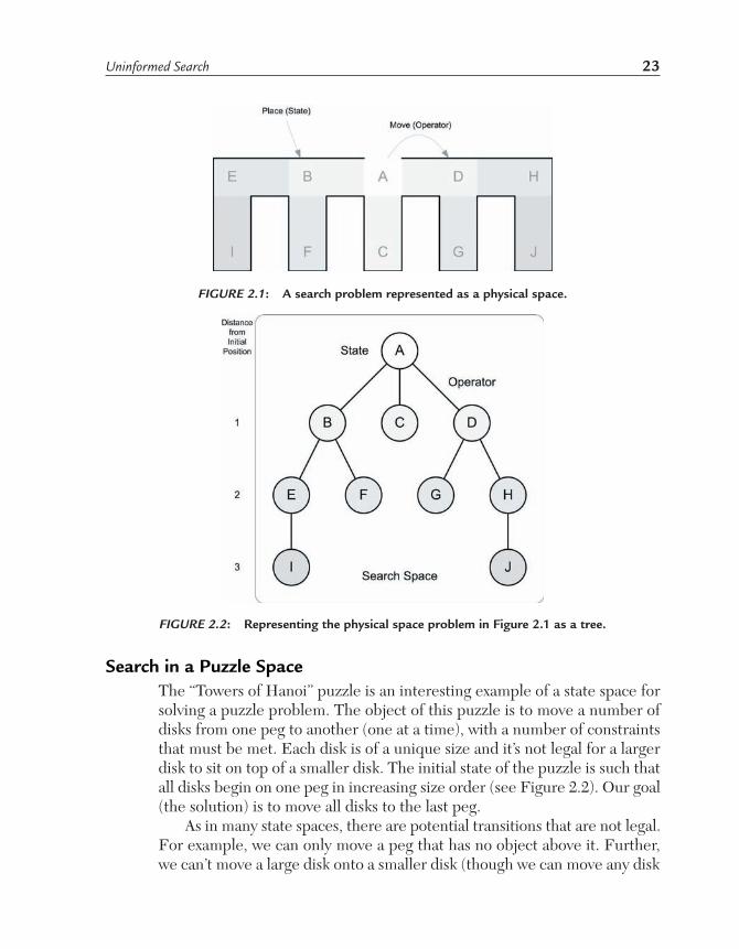
Search in a Physical SpaceLet’s consider a simple search problem in physical space (Figure 2.1). Our initial position is ‘A’ from which there are three possible actions that lead to position ‘B,’ ‘C,’ or ‘D.’ Places, or states, are marked by letters. At each place, there’s an opportunity for a decision, or action. The action (also called an operator) is simply a legal move between one place and another. Implied in this exercise is a goal state, or a physical location that we’re seeking.
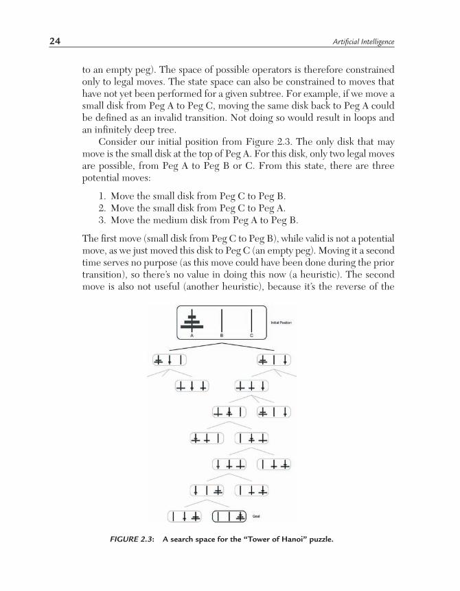
This search space (shown in Figure 2.1) can be reduced to a tree structure as illustrated in Figure 2.2. The search space has been minimized here to the necessary places on the physical map (states) and the transitions that are possible between the states (application of operators). Each node in the tree is a physical location and the arcs between nodes are the legal moves. The depth of the tree is the distance from the initial position.
Uninformed Search 23
Search in a Puzzle SpaceThe “Towers of Hanoi” puzzle is an interesting example of a state space for solving a puzzle problem. The object of this puzzle is to move a number of disks from one peg to another (one at a time), with a number of constraints that must be met. Each disk is of a unique size and it’s not legal for a larger disk to sit on top of a smaller disk. The initial state of the puzzle is such that all disks begin on one peg in increasing size order (see Figure 2.2). Our goal (the solution) is to move all disks to the last peg.
As in many state spaces, there are potential transitions that are not legal. For example, we can only move a peg that has no object above it. Further, we can’t move a large disk onto a smaller disk (though we can move any disk
FIGURE 2.1: A search problem represented as a physical space.
FIGURE 2.2: Representing the physical space problem in Figure 2.1 as a tree.
24 Artificial Intelligence
to an empty peg). The space of possible operators is therefore constrained only to legal moves. The state space can also be constrained to moves that have not yet been performed for a given subtree. For example, if we move a small disk from Peg A to Peg C, moving the same disk back to Peg A could be defined as an invalid transition. Not doing so would result in loops and an infinitely deep tree.
Consider our initial position from Figure 2.3. The only disk that may move is the small disk at the top of Peg A. For this disk, only two legal moves are possible, from Peg A to Peg B or C. From this state, there are three potential moves:
1. Move the small disk from Peg C to Peg B.2. Move the small disk from Peg C to Peg A.3. Move the medium disk from Peg A to Peg B.
The first move (small disk from Peg C to Peg B), while valid is not a potential move, as we just moved this disk to Peg C (an empty peg). Moving it a second time serves no purpose (as this move could have been done during the prior transition), so there’s no value in doing this now (a heuristic). The second move is also not useful (another heuristic), because it’s the reverse of the
FIGURE 2.3: A search space for the “Tower of Hanoi” puzzle.

Uninformed Search 25
previous move. This leaves one valid move, the medium disk from Peg A to Peg B. The possible moves from this state become more complicated, because valid moves are possible that move us farther away from the solution.
TIP A heuristic is a simple or efficient rule for solving a given problem or making a decision.
When our sequence of moves brings us from the initial position to the goal, we have a solution. The goal state in itself is not interesting, but instead what’s interesting is the sequence of moves that brought us to the goal state. The collection of moves (or solution), done in the proper order, is in essence a plan for reaching the goal. The plan for this configuration of the puzzle can be identified by starting from the goal position and backtracking to the initial position.
Search in an Adversarial Game SpaceAn interesting use of search spaces is in games. Also known as game trees, these structures enumerate the possible moves by each player allowing the search algorithm to find an effective strategy for playing and winning the game.
NOTE The topic of adversarial search in game trees is explored in Chapter 4.
Consider a game tree for the game of Chess. Each possible move is provided for each possible configuration (placement of pieces) of the Chess board. But since there are 10120 possible configurations of a Chess board, a game tree to document the search space would not be feasible. Heuristic search, which must be applied here, will be discussed in Chapter 3.
Let’s now look at a much simpler game that can be more easily represented in a game tree. The game of Nim is a two-player game where each player takes turns removing objects from one or more piles. The player required to take the last object loses the game.
Nim has been studied mathematically and solved in many different variations. For this reason, the player who will win can be calculated based upon the number of objects, piles, and who plays first in an optimally played game.
NOTE The game of Nim is said to have originated in China, but can be traced to Germany as the word nimm can be translated as take. A complete mathematical theory of Nim was created by Charles Bouton in 1901. [Bouton 1901]

26 Artificial Intelligence
Let’s walk through an example to see how Nim is played. We’ll begin with a single small pile to limit the number of moves that are required. Figure 2.4 illustrates a short game with a pile of six objects. Each player may take one, two, or three objects from the pile. In this example, Player-1 starts the game, but ends the game with a loss (is required to take the last object which results in a loss in the misère form of the game). Had Player-1 taken 3 in its second move, Player-2 would have been left with one resulting in a win for Player-1.
A game tree makes this information visible, as illustrated in Figure 2.5. Note in the tree that Player-1 must remove one from the pile to continue the game. If Player-1 removes two or three from the pile, Player-2 can win if playing optimally. The shaded nodes in the tree illustrate losing positions for the player that must choose next (and in all cases, the only choice left is to take the only remaining object).
Note that the depth of the tree determines the length of the game (number of moves). It’s implied in the tree that the shaded node is the final move to be made, and the player that makes this move loses the game. Also note the size of the tree. In this example, using six objects, a total of 28 nodes is required. If we increase our tree to illustrate a pile of seven objects, the tree increases to 42 nodes. With eight objects, three balloons to 100 nodes. Fortunately, the tree can be optimized by removing duplicate subtrees, resulting in a much smaller tree.
FIGURE 2.4: A sample game of Nim with a pile of six objects.

Uninformed Search 27
TREES, GRAPHS, AND REPRESENTATION
A short tour of trees and graphs and their terminology is in order before exploring the various uninformed search methods.
A graph is a finite set of vertices (or nodes) that are connected by edges (or arcs). A loop (or cycle) may exist in a graph, where an arc (or edge) may lead back to the original node. Graphs may be undirected where arcs do not imply a direction, or they may be directed (called a digraph) where a direction is implicit in the arc. An arc can also carry a weight, where a cost can be associated with a path.
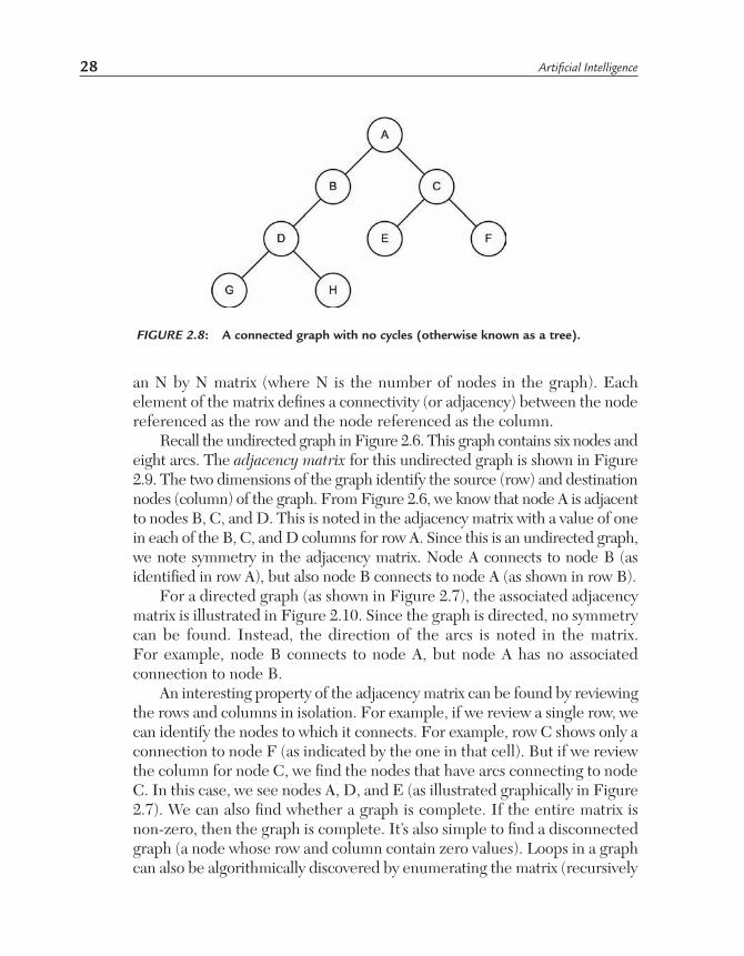
Each of these graphs also demonstrates the property of connectivity. Both graphs are connected because every pair of nodes is connected by a path. If every node is connected to every node by an arc, the graph is complete. One special connected graph is called a tree, but it must contain no cycles.
Building a representation of a graph is simple and one of the most common representations is the adjacency matrix. This structure is simply
FIGURE 2.5: A complete Nim game tree for six objects in one pile.
FIGURE 2.6: An example of an undirected graph containing six nodes and eight arcs.
FIGURE 2.7: An example of a directed graph containing six edges and nine arcs.
28 Artificial Intelligence
an N by N matrix (where N is the number of nodes in the graph). Each element of the matrix defines a connectivity (or adjacency) between the node referenced as the row and the node referenced as the column.
Recall the undirected graph in Figure 2.6. This graph contains six nodes and eight arcs. The adjacency matrix for this undirected graph is shown in Figure 2.9. The two dimensions of the graph identify the source (row) and destination nodes (column) of the graph. From Figure 2.6, we know that node A is adjacent to nodes B, C, and D. This is noted in the adjacency matrix with a value of one in each of the B, C, and D columns for row A. Since this is an undirected graph, we note symmetry in the adjacency matrix. Node A connects to node B (as identified in row A), but also node B connects to node A (as shown in row B).
For a directed graph (as shown in Figure 2.7), the associated adjacency matrix is illustrated in Figure 2.10. Since the graph is directed, no symmetry can be found. Instead, the direction of the arcs is noted in the matrix. For example, node B connects to node A, but node A has no associated connection to node B.
An interesting property of the adjacency matrix can be found by reviewing the rows and columns in isolation. For example, if we review a single row, we can identify the nodes to which it connects. For example, row C shows only a connection to node F (as indicated by the one in that cell). But if we review the column for node C, we find the nodes that have arcs connecting to node C. In this case, we see nodes A, D, and E (as illustrated graphically in Figure 2.7). We can also find whether a graph is complete. If the entire matrix is non-zero, then the graph is complete. It’s also simple to find a disconnected graph (a node whose row and column contain zero values). Loops in a graph can also be algorithmically discovered by enumerating the matrix (recursively
FIGURE 2.8: A connected graph with no cycles (otherwise known as a tree).

Uninformed Search 29
following all paths looking for the initial node).In the simple case, the values of the adjacency matrix simply define the
connectivity of nodes in the graph. In weighted graphs, where arcs may not all be equal, the value in a cell can identify the weight (cost, or distance). We’ll explore examples of this technique in the review of neural network construction (Chapter 11).
Adjacency lists are also a popular structure where each node contains a list of the nodes to which it connects. If the graph is sparse, this representation can require less space.
UNINFORMED SEARCHThe uninformed search methods offer a variety of techniques for graph search, each with its own advantages and disadvantages. These methods are explored here with discussion of their characteristics and complexities.
Big-O notation will be used to compare the algorithms. This notation defines the asymptotic upper bound of the algorithm given the depth (d) of the tree and the branching factor, or the average number of branches (b) from each node. There are a number of common complexities that exist for search algorithms. These are shown in Table 2.1.
Table 2.1: Common orders of search functions.
O-Notation OrderO(1) Constant (regardless of the number of nodes)
FIGURE 2.9: Adjacency matrix for the undirected graph shown in Figure 2.6.
FIGURE 2.10: Adjacency matrix for the directed graph (digraph) shown in Figure 2.7.

30 Artificial Intelligence
O(n) Linear (consistent with the number of nodes)O(log n) LogarithmicO(n2) QuadraticO(cn) GeometricO(n!) Combinatorial
Big-O notation provides a worst-case measure of the complexity of a search algorithm and is a common comparison tool for algorithms. We’ll compare the search algorithms using space complexity (measure of the memory required during the search) and time complexity (worst-case time required to find a solution). We’ll also review the algorithm for completeness (can the algorithm find a path to a goal node if it’s present in the graph) and optimality (finds the lowest cost solution available).
Helper APIsA number of helper APIs will be used in the source code used to demonstrate the search functions. These are shown below in Listing 2.1.
LISTING 2.1: Helper APIs for the search functions.
/* Graph API */graph_t *createGraph (int nodes );void destroyGraph (graph_t *g_p );void addEdge (graph_t *g_p, int from, int to, int value );int getEdge (graph_t *g_p, int from, int to );/* Stack API */stack_t *createStack (int depth );void destroyStack (stack_t *s_p );void pushStack (stack_t *s_p, int value );int popStack (stack_t *s_p );int isEmptyStack (stack_t *s_p );/* Queue API */queue_t *createQueue (int depth );void destroyQueue (queue_t *q_p );void enQueue (queue_t *q_p, int value );int deQueue (queue_t *q_p );int isEmptyQueue (queue_t *q_p );/* Priority Queue API */pqueue_t *createPQueue (int depth );

Uninformed Search 31
void destroyPQueue (pqueue_t *q_p );void enPQueue (pqueue_t *q_p, int value, int cost );void dePQueue (pqueue_t *q_p, int *value, int *cost );int isEmptyPQueue (pqueue_t *q_p );int isFullPQueue (pqueue_t *q_p );
O
N THE CD
The helper functions can be found on the CD-ROM at ./software/common.
General Search ParadigmsBefore we discuss some of the uninformed search methods, let’s look at two simple general uninformed search methods.
The first is called ‘Generate and Test.’ In this method, we generate a potential solution and then check it against the solution. If we’ve found the solution, we’re done, otherwise, we repeat by trying another potential solution. This is called ‘Generate and Test’ because we generate a potential solution, and then test it. Without a proper solution, we try again. Note here that we don’t keep track of what we’ve tried before; we just plow ahead with potential solutions, which is a true blind search.
Another option is called ‘Random Search’ which randomly selects a new state from the current state (by selecting a given valid operator and applying it). If we reach the goal state, then we’re done. Otherwise, we randomly select another operator (leading to a new state) and continue.
Random search and the ‘Generate and Test’ method are truly blind methods of search. They can get lost, get caught in loops, and potentially never find a solution even though one exists within the search space.
Let’s now look at some search methods that while blind, can find a solution (if one exists) even if it takes a long period of time.
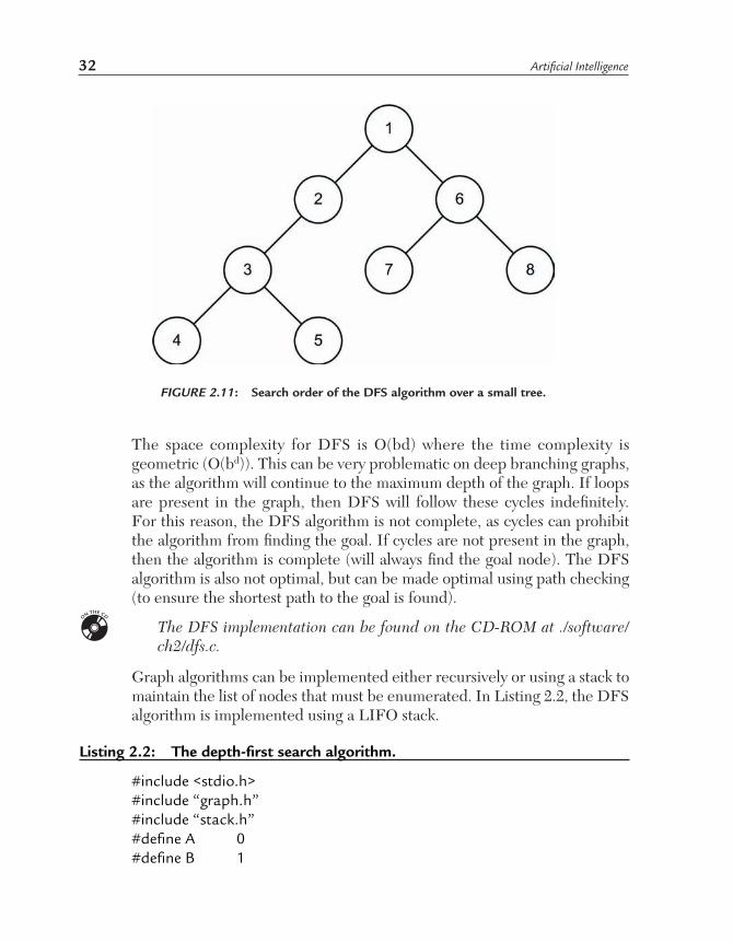
Depth-First Search (DFS)The Depth-First Search (DFS) algorithm is a technique for searching a graph that begins at the root node, and exhaustively searches each branch to its greatest depth before backtracking to previously unexplored branches (Figure 2.11 illustrates this search order). Nodes found but yet to be reviewed are stored in a LIFO queue (also known as a stack).
NOTE A stack is a LIFO (Last-In-First-Out) container of objects. Similar to a stack of paper, the last item placed on the top is the first item to be removed.
32 Artificial Intelligence
The space complexity for DFS is O(bd) where the time complexity is geometric (O(bd)). This can be very problematic on deep branching graphs, as the algorithm will continue to the maximum depth of the graph. If loops are present in the graph, then DFS will follow these cycles indefinitely. For this reason, the DFS algorithm is not complete, as cycles can prohibit the algorithm from finding the goal. If cycles are not present in the graph, then the algorithm is complete (will always find the goal node). The DFS algorithm is also not optimal, but can be made optimal using path checking (to ensure the shortest path to the goal is found).
O
N THE CD The DFS implementation can be found on the CD-ROM at ./software/
ch2/dfs.c.
Graph algorithms can be implemented either recursively or using a stack to maintain the list of nodes that must be enumerated. In Listing 2.2, the DFS algorithm is implemented using a LIFO stack.
Listing 2.2: The depth-first search algorithm.
#include <stdio.h>#include “graph.h”#include “stack.h”#define A 0#define B 1
FIGURE 2.11: Search order of the DFS algorithm over a small tree.
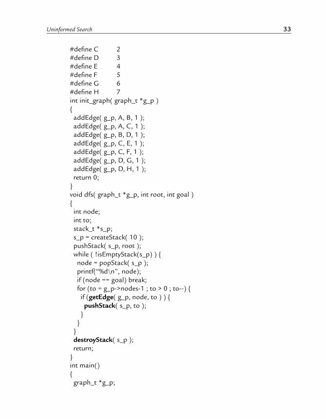
Uninformed Search 33
#define C 2#define D 3#define E 4#define F 5#define G 6#define H 7int init_graph( graph_t *g_p ){ addEdge( g_p, A, B, 1 ); addEdge( g_p, A, C, 1 ); addEdge( g_p, B, D, 1 ); addEdge( g_p, C, E, 1 ); addEdge( g_p, C, F, 1 ); addEdge( g_p, D, G, 1 ); addEdge( g_p, D, H, 1 ); return 0;}void dfs( graph_t *g_p, int root, int goal ){ int node; int to; stack_t *s_p; s_p = createStack( 10 ); pushStack( s_p, root ); while ( !isEmptyStack(s_p) ) { node = popStack( s_p ); printf(“%d\n”, node); if (node == goal) break; for (to = g_p->nodes-1 ; to > 0 ; to--) { if (getEdge( g_p, node, to ) ) { pushStack( s_p, to ); } } } destroyStack( s_p ); return;}int main(){ graph_t *g_p;

34 Artificial Intelligence
g_p = createGraph( 8 ); init_graph( g_p ); dfs( g_p, 0, 5 ); destroyGraph( g_p ); return 0;}
TIP A search algorithm is characterized as exhaustive when it can search every node in the graph in search of the goal. If the goal is not present in the graph, the algorithm will terminate, but will search each and every node in a systematic way.
Depth-Limited Search (DLS)Depth-Limited Search (DLS) is a modification of depth-first search that minimizes the depth that the search algorithm may go. In addition to starting with a root and goal node, a depth is provided that the algorithm will not descend below (see Listing 2.3). Any nodes below that depth are omitted from the search. This modification keeps the algorithm from indefinitely cycling by halting the search after the pre-imposed depth. Figure 2.12 illustrates this search with a depth of two (no nodes deeper than level two are searched).
O
N THE CD
The DLS implementation can be found on the CD-ROM at ./software/ch2/dls.c.
Listing 2.3: The depth-limited search algorithm.
#include <stdio.h>#include “graph.h”#include “stack.h”#define A 0#define B 1#define C 2#define D 3#define E 4#define F 5#define G 6#define H 7int init_graph( graph_t *g_p ){

Uninformed Search 35
addEdge( g_p, A, B, 1 ); addEdge( g_p, A, C, 1 ); addEdge( g_p, B, D, 1 ); addEdge( g_p, C, E, 1 ); addEdge( g_p, C, F, 1 ); addEdge( g_p, D, G, 1 ); addEdge( g_p, D, H, 1 ); return 0;}void dls( graph_t *g_p, int root, int goal, int limit ){ int node, depth, to; stack_t *s_p, *sd_p; s_p = createStack( 10 ); sd_p = createStack( 10 ); pushStack( s_p, root ); pushStack( sd_p, 0 ); while ( !isEmptyStack(s_p) ) { node = popStack( s_p ); depth = popStack( sd_p ); printf(“%d (depth %d)\n”, node, depth); if (node == goal) break; if (depth < limit) { for (to = g_p->nodes-1 ; to > 0 ; to--) { if (getEdge( g_p, node, to ) ) { pushStack( s_p, to ); pushStack( sd_p, depth+1 ); } } } } destroyStack( s_p ); destroyStack( sd_p ); return;}int main(){ graph_t *g_p; g_p = createGraph( 8 ); init_graph( g_p );

36 Artificial Intelligence
dls( g_p, 0, 5, 2 ); destroyGraph( g_p ); return 0;}
While the algorithm does remove the possibility of infinitely looping in the graph, it also reduces the scope of the search. If the goal node had been one of the nodes marked ‘X’, it would not have been found, making the search algorithm incomplete. The algorithm can be complete if the search depth is that of the tree itself (in this case d is three). The technique is also not optimal since the first path may be found to the goal instead of the shortest path.
The time and space complexity of depth-limited search is similar to DFS, from which this algorithm is derived. Space complexity is O(bd) and time complexity is O(bd), but d in this case is the imposed depth of the search and not the maximum depth of the graph.
Iterative Deepening Search (IDS)Iterative Deepening Search (IDS) is a derivative of DLS and combines the features of depth-first search with that of breadth-first search. IDS operates by performing DLS searches with increased depths until the goal is found.
FIGURE 2.13: Iterating increased depth searches with IDS.
FIGURE 2.12: Search order for a tree using depth-limited search (depth = two).

Uninformed Search 37
The depth begins at one, and increases until the goal is found, or no further nodes can be enumerated (see Figure 2.13).
As shown in Figure 2.13, IDS combines depth-first search with breadth-first search. By minimizing the depth of the search, we force the algorithm to also search the breadth of the graph. If the goal is not found, the depth that the algorithm is permitted to search is increased and the algorithm is started again. The algorithm, shown in Listing 2.4, begins with a depth of one.
LISTING 2.4: The iterative deepening-search algorithm.
#include <stdio.h>#include “graph.h”#include “stack.h”#define A 0#define B 1#define C 2#define D 3#define E 4#define F 5#define G 6#define H 7int init_graph( graph_t *g_p ){ addEdge( g_p, A, B, 1 ); addEdge( g_p, A, C, 1 ); addEdge( g_p, B, D, 1 ); addEdge( g_p, C, E, 1 ); addEdge( g_p, C, F, 1 ); addEdge( g_p, D, G, 1 ); addEdge( g_p, D, H, 1 ); return 0;}int dls( graph_t *g_p, int root, int goal, int limit ){ int node, depth; int to; stack_t *s_p, *sd_p; s_p = createStack( 10 ); sd_p = createStack( 10 ); pushStack( s_p, root );

38 Artificial Intelligence
pushStack( sd_p, 0 ); while ( !isEmptyStack(s_p) ) { node = popStack( s_p ); depth = popStack( sd_p ); printf(“%d (depth %d)\n”, node, depth); if (node == goal) return 1; if (depth < limit) { for (to = g_p->nodes-1 ; to > 0 ; to--) { if (getEdge( g_p, node, to ) ) { pushStack( s_p, to ); pushStack( sd_p, depth+1 ); } } } } destroyStack( s_p ); destroyStack( sd_p ); return 0;}int main(){ graph_t *g_p; int status, depth; g_p = createGraph( 8 ); init_graph( g_p ); depth = 1; while (1) { status = dls( g_p, 0, 5, depth ); if (status == 1) break; else depth++; } destroyGraph( g_p ); return 0;}
O
N THE CD
The IDS implementation can be found on the CD-ROM at ./software/ch2/ids.c.
IDS is advantageous because it’s not susceptible to cycles (a characteristic of DLS, upon which it’s based). It also finds the goal nearest to the root node,

Uninformed Search 39
as does the BFS algorithm (which will be detailed next). For this reason, it’s a preferred algorithm when the depth of the solution is not known.
The time complexity for IDS is identical to that of DFS and DLS, O(bd). Space complexity of IDS is O(bd).
Unlike DFS and DLS, IDS is will always find the best solution and therefore, it is both complete and optimal.
Breadth-First Search (BFS)In Breadth-First Search (BFS), we search the graph from the root node in order of the distance from the root. Because the order search is nearest the root, BFS is guaranteed to find the best possible solution (shallowest) in a non-weighted graph, and is therefore also complete. Rather than digging deep down into the graph, progressing further and further from the root (as is the case with DFS), BFS checks each node nearest the root before descending to the next level (see Figure 2.14).
The implementation of BFS uses a FIFO (first-in-first-out) queue, differing from the stack (LIFO) implementation for DFS. As new nodes are found to be searched, these nodes are checked against the goal, and if the goal is not found, the new nodes are added to the queue. To continue the search, the oldest node is dequeued (FIFO order). Using FIFO order for new node search, we always check the oldest nodes first, resulting in breadth-first review (see Listing 2.5).
LISTING 2.5: The breadth-first search algorithm.
#include <stdio.h>#include “graph.h”#include “queue.h”#define A 0
FIGURE 2.14: Search order of the breadth-first search algorithm.

40 Artificial Intelligence
#define B 1#define C 2#define D 3#define E 4#define F 5#define G 6#define H 7int init_graph( graph_t *g_p ){ addEdge( g_p, A, B, 1 ); addEdge( g_p, A, C, 1 ); addEdge( g_p, B, D, 1 ); addEdge( g_p, C, E, 1 ); addEdge( g_p, C, F, 1 ); addEdge( g_p, D, G, 1 ); addEdge( g_p, D, H, 1 ); return 0;}void bfs( graph_t *g_p, int root, int goal ){ int node; int to; queue_t *q_p; q_p = createQueue( 10 ); enQueue( q_p, root ); while ( !isEmptyQueue(q_p) ) { node = deQueue( q_p ); printf(“%d\n”, node); if (node == goal) break; for (to = g_p->nodes-1 ; to > 0 ; to--) { if (getEdge( g_p, node, to ) ) { enQueue( q_p, to ); } } } destroyQueue( q_p ); return;}int main(){

Uninformed Search 41
graph_t *g_p; g_p = createGraph( 8 ); init_graph( g_p ); bfs( g_p, 0, 7 ); destroyGraph( g_p ); return 0;}
O
N THE CD
The BFS implementation can be found on the CD-ROM at ./software/ch2/bfs.c.
The disadvantage of BFS is that each node that is searched is required to be stored (space complexity is O(bd)). The entire depth of the tree does not have to be searched, so d in this context is the depth of the solution, and not the maximum depth of the tree. Time complexity is also O(bd).
TIP In practical implementations of BFS, and other search algorithms, a closed list is maintained that contains those nodes in the graph that have been visited. This allows the algorithm to efficiently search the graph without re-visiting nodes. In implementations where the graph is weighted, keeping a closed list is not possible.
FIGURE 2.15: Bidirectional search meeting in the middle at node H.

42 Artificial Intelligence
Bidirectional SearchThe Bidirectional Search algorithm is a derivative of BFS that operates by performing two breadth-first searches simultaneously, one beginning from the root node and the other from the goal node. When the two searches meet in the middle, a path can be reconstructed from the root to the goal. The searches meeting is determined when a common node is found (a node visited by both searches, see Figure 2.15). This is accomplished by keeping a closed list of the nodes visited.
Bidirectional search is an interesting idea, but requires that we know the goal that we’re seeking in the graph. This isn’t always practical, which limits the application of the algorithm. When it can be determined, the algorithm has useful characteristics. The time and space complexity for bidirectional search is O(bd/2), since we’re only required to search half of the depth of the tree. Since it is based on BFS, bidirectional search is both complete and optimal.
Uniform-Cost Search (UCS)One advantage of BFS is that it always finds the shallowest solution. But consider the edge having a cost associated with it. The shallowest solution may not be the best, and a deeper solution with a reduced path cost would be better (for example, see Figure 2.16). Uniform -Cost Search (UCS) can be applied to find the least-cost path through a graph by maintaining an ordered list of nodes in order of descending cost. This allows us to evaluate the least cost path first
FIGURE 2.16: An example graph where choosing the lowest cost path for the first node (A->C) may not result in the best overall path through the graph (A->B->E).

Uninformed Search 43
TIP Uniform-cost search is an uninformed search method because no heuristic is actually used. The algorithm measures the actual cost of the path without attempting to estimate it.
The algorithm for UCS uses the accumulated path cost and a priority queue to determine the path to evaluate (see Listing 2.6). The priority queue (sorted from least cost to greatest) contains the nodes to be evaluated. As node children are evaluated, we add their cost to the node with the aggregate sum of the current path. This node is then added to the queue, and when all children have been evaluated, the queue is sorted in order of ascending cost. When the first element in the priority queue is the goal node, then the best solution has been found.
LISTING 2.6: The uniform-cost search algorithm.
#include <stdio.h>#include “graph.h”#include “pqueue.h”#define A 0#define B 1#define C 2#define D 3#define E 4int init_graph( graph_t *g_p ){ addEdge( g_p, A, B, 5 ); addEdge( g_p, A, C, 1 ); addEdge( g_p, A, D, 2 ); addEdge( g_p, B, E, 1 ); addEdge( g_p, C, E, 7 ); addEdge( g_p, D, E, 5 ); return 0;}void ucs( graph_t *g_p, int root, int goal ){ int node, cost, child_cost; int to; pqueue_t *q_p; q_p = createPQueue( 7 ); enPQueue( q_p, root, 0 ); while ( !isEmptyPQueue(q_p) ) {
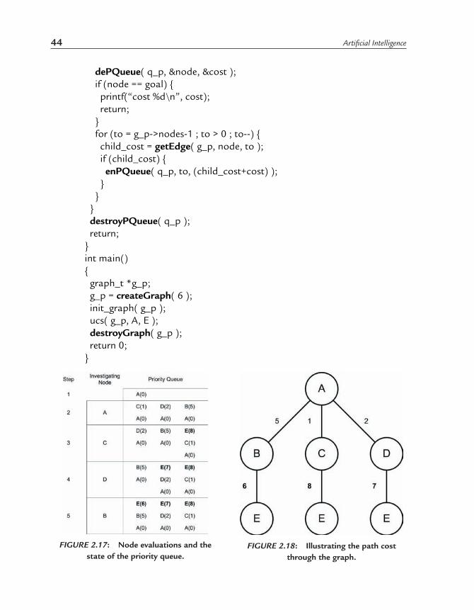
44 Artificial Intelligence
dePQueue( q_p, &node, &cost ); if (node == goal) { printf(“cost %d\n”, cost); return; } for (to = g_p->nodes-1 ; to > 0 ; to--) { child_cost = getEdge( g_p, node, to ); if (child_cost) { enPQueue( q_p, to, (child_cost+cost) ); } } } destroyPQueue( q_p ); return;}int main(){ graph_t *g_p; g_p = createGraph( 6 ); init_graph( g_p ); ucs( g_p, A, E ); destroyGraph( g_p ); return 0;}
FIGURE 2.17: Node evaluations and the state of the priority queue.
FIGURE 2.18: Illustrating the path cost through the graph.

Uninformed Search 45
ON THE CD
The UCS implementation can be found on the CD-ROM at ./software/ch2/ucs.c.
The UCS algorithm is easily demonstrated using our example graph in Figure 2.16. Figure 2.17 shows the state of the priority queue as the nodes are evaluated. At step one, the initial node has been added to the priority queue, with a cost of zero. At step two, each of the three connected nodes are evaluated and added to the priority queue. When no further children are available to evaluate, the priority queue is sorted to place them in ascending cost order.
At step three, children of node C are evaluated. In this case, we find the desired goal (E), but since its accumulated path cost is eight, it ends up at the end of the queue. For step four, we evaluate node D and again find the goal node. The path cost results in seven, which is still greater than our B node in the queue. Finally, at step five, node B is evaluated. The goal node is found again, with a resulting path cost of six. The priority queue now contains the goal node at the top, which means at the next iteration of the loop, the algorithm will exit with a path of A->B->E (working backwards from the goal node to the initial node).
To limit the size of the priority queue, it’s possible to prune entries that are redundant. For example, at step 4 in Figure 2.17, the entry for E(8) could have been safely removed, as another path exists that has a reduced cost (E(7)).
The search of the graph is shown in Figure 2.18, which identifies the path cost at each edge of the graph. The path cost shown above the goal node (E) makes it easy to see the least-cost path through the graph, even when it’s not apparent from the initial node.
UCS is optimal and can be complete, but only if the edge costs are non-negative (the summed path cost always increases). Time and space complexity are the same as BFS, O(bd) for each, as it’s possible for the entire tree to be evaluated.
IMPROVEMENTS
One of the basic problems with traditional DFS and BFS is that they lack a visited list (a list of nodes that have already been evaluated). This modification makes the algorithms complete, by ignoring cycles and only following paths that have not yet been followed. For BFS, keeping a visited list can reduce the search time, but for DFS, the algorithm can be made complete.

46 Artificial Intelligence
ALGORITHM ADVANTAGES
Each of the algorithms has advantages and disadvantages based on the graph to be searched. For example, if the branching factor of the graph is small, then BFS is the best choice. If the tree is deep, but a solution is known to be shallow in the graph, then IDS is a good choice. If the graph is weighted, then UCS should be used as it will always find the best solution where DFS and BFS will not.
CHAPTER SUMMARYUninformed search algorithms are a class of graph search algorithms that exhaustively search for a node without the use of a heuristic to guide the search. Search algorithms are of interest in AI because many problems can be reduced to simple search problems in a state space. The state space consists of states (nodes) and operators (edges), allowing the state space to be represented as a graph. Examples range from graphs of physical spaces to massive game trees such as are possible with the game of Chess.
The depth-first search algorithm operates by evaluating branches to their maximum depth, and then backtracking to follow unvisited branches. Depth-limited search (DLS) is based on DFS, but restricts the depth of the search. Iterative-deepening search (IDS) uses DLS, but continually increases the search depth until the solution is found.
The breadth-first search (BFS) algorithm searches with increasing depth from the root (searches all nodes with depth one, then all nodes with depth two, etc.). A special derivative algorithm of BFS, bidirectional search (BIDI), performs two simultaneous searches. Starting at the root node and the goal node, BIDI performs two BFS searches in search of the middle. Once a common node is found in the middle, a path exists between the root and goal nodes.
The uniform-cost search (UCS) algorithm is ideal for weight graphs (graphs whose edges have costs associated with them). UCS evaluates a graph using a priority queue that is ordered in path cost to the particular node. It’s based on the BFS algorithm and is both complete and optimal.
ALGORITHMS SUMMARYTable 2.2: Summary of the uninformed algorithms and their characteristics.

Uninformed Search 47
Algorithm Time Space Optimal Complete DerivativeDFS O(bm) O(bm) No NoDLS O(bl) O(bl) No No DFSIDS O(bd) O(bd) Yes No DLSBFS O(bd) O(bd) Yes YesBIDI O(bd/2) O(bd/2) Yes Yes BFSUCS O(bd) O(bd) Yes Yes BFSb, branching factord, tree depth of the solutionm, tree depthl, search depth limit
REFERENCES
[Bouton 1901] “Nim, a game with a complete mathematical theory,” Ann, Math, Princeton 3, 35-39, 1901-1902.
EXERCISES
1. What is uninformed (or blind) search and how does it differ from informed (or heuristic) search?
2. The graph structure is ideal for general state space representation. Explain why and define the individual components.
3. Define the queuing structures used in DFS and BFS and explain why each uses their particular style.
4. What is the definition of tree depth?5. What is the definition of the branching factor?6. What are time and space complexity and why are they useful as metrics
for graph search?7. If an algorithm always finds a solution in a graph, what is this property
called? If it always finds the best solution, what is this characteristic?8. Considering DFS and BFS, which algorithm will always find the best
solution for a non-weighted graph?9. Use the DFS and BFS algorithms to solve the Towers of Hanoi problem.
Which performs better and why?10. Provide the search order for the nodes shown in Figure 2.19 for DFS, BFS,
DLS (d=2), IDS (start depth = 1), and BIDI (start node A, goal node I).

48 Artificial Intelligence
11. In general, IDS is better than DFS. Draw a graph where this is not the case.
12. In general, IDS is not complete. Why?13. Identify a major disadvantage of bidirectional search.14. Using the UCS algorithm, find the shortest path from A to F in Figure 2.20.
FIGURE 2.19: Example graph. FIGURE 2.20: Example weighted graph.

C h a p t e r 3 INFORMED SEARCH
In Chapter 2, we explored the uninformed search methods such as depth-first and breadth-first search. These methods operate in a brute-force fashion and are subsequently inefficient. In contrast, this chapter
will present the informed search methods. These methods incorporate a heuristic, which is used to determine the quality of any state in the search space. In a graph search, this results in a strategy for node expansion (which node should be evaluated next). A variety of informed search methods will be investigated and, as with uninformed methods, compared using a common set of metrics.
NOTE A heuristic is a rule of thumb that may help solve a given problem. Heuristics take problem knowledge into consideration to help guide the search within the domain.
INFORMED SEARCH
In this chapter, we’ll explore a number of informed search methods, including best-first search, a-star search, iterative improvement algorithms such as hill climbing and simulated annealing, and finally, constraint satisfaction. We’ll demonstrate each with a sample problem and illustrate the heuristics used.
50 Artificial Intelligence
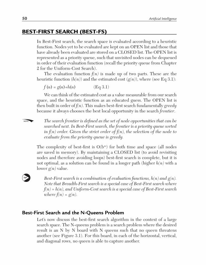
BEST-FIRST SEARCH (BEST-FS)
In Best-First search, the search space is evaluated according to a heuristic function. Nodes yet to be evaluated are kept on an OPEN list and those that have already been evaluated are stored on a CLOSED list. The OPEN list is represented as a priority queue, such that unvisited nodes can be dequeued in order of their evaluation function (recall the priority queue from Chapter 2 for the Uniform-Cost Search).
The evaluation function f(n) is made up of two parts. These are the heuristic function (h(n)) and the estimated cost (g(n)), where (see Eq 3.1):
f (n) = g(n)+h(n) (Eq 3.1)
We can think of the estimated cost as a value measurable from our search space, and the heuristic function as an educated guess. The OPEN list is then built in order of f(n). This makes best-first search fundamentally greedy because it always chooses the best local opportunity in the search frontier.
NOTE The search frontier is defined as the set of node opportunities that can be searched next. In Best-First search, the frontier is a priority queue sorted in f(n) order. Given the strict order of f(n), the selection of the node to evaluate from the priority queue is greedy.
The complexity of best-first is O(bm) for both time and space (all nodes are saved in memory). By maintaining a CLOSED list (to avoid revisiting nodes and therefore avoiding loops) best-first search is complete, but it is not optimal, as a solution can be found in a longer path (higher h(n) with a lower g(n) value.
TIP Best-First search is a combination of evaluation functions, h(n) and g(n). Note that Breadth-First search is a special case of Best-First search where f(n) = h(n), and Uniform-Cost search is a special case of Best-First search where f(n) = g(n).
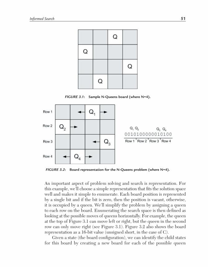
Best-First Search and the N-Queens ProblemLet’s now discuss the best-first search algorithm in the context of a large search space. The N-queens problem is a search problem where the desired result is an N by N board with N queens such that no queen threatens another (see Figure 3.1). For this board, in each of the horizontal, vertical, and diagonal rows, no queen is able to capture another.
Informed Search 51
An important aspect of problem solving and search is representation. For this example, we’ll choose a simple representation that fits the solution space well and makes it simple to enumerate. Each board position is represented by a single bit and if the bit is zero, then the position is vacant, otherwise, it is occupied by a queen. We’ll simplify the problem by assigning a queen to each row on the board. Enumerating the search space is then defined as looking at the possible moves of queens horizontally. For example, the queen at the top of Figure 3.1 can move left or right, but the queen in the second row can only move right (see Figure 3.1). Figure 3.2 also shows the board representation as a 16-bit value (unsigned short, in the case of C).
Given a state (the board configuration), we can identify the child states for this board by creating a new board for each of the possible queen
FIGURE 3.1: Sample N-Queens board (where N=4).
FIGURE 3.2: Board representation for the N-Queens problem (where N=4).

52 Artificial Intelligence
position changes, given horizontal movement only. For Figure 3.2, this board configuration can result in six new child states (a single queen change position in each). Note that since we maintain a closed list, board configurations that have already been evaluated are not generated, resulting in a small tree and more efficient search.
For the heuristic, we’ll use the node’s depth in the tree for h(n), and the number of conflicts (number of queens that could capture another) for g(n).
Best-First Search ImplementationLet’s now look at a simple implementation of Best-First search in the C language. We’ll present the two major functions that make up this search algorithm; the first is best_fs, which is the main loop of the algorithm. The second function, generateChildNodes, builds out the possible states (board configurations) given the current state.
Our main function (best_fs) is the OPEN list enumerator and solution tester. Prior to calling this function, our OPEN list (priority queue) and CLOSED list have been created. The root node, our initial board configuration, has been placed on the OPEN list. The best_fs function (see Listing 3.1) then dequeues the next node from the open list (best f(n)) If this node has a g(n) (number of conflicts) of zero, then a solution has been found, and we exit.
LISTING 3.1: The Best-Search first main function.
void best_fs ( pqueue_t *open_pq_p, queue_t *closed_q_p ){ node_t *node_p; int cost; /* Enumerate the Open list */ while ( !isEmptyPQueue (open_pq_p) ) { dePQueue ( open_pq_p, (int *)&node_p, &cost ); /* Solution found? */ if (node_p->g == 0) { printf(“Found Solution (depth %d):\n”, node_p->h); emitBoard ( node_p ); break; } generateChildNodes( open_pq_p, closed_q_p, node_p );

Informed Search 53
} return;}
Note in Listing 3.1 that while cost is the f(n), we check g(n) to determine whether a solution is found. This is because f(n) may be non-zero since it includes the depth of the solution (h(n)).
O
N THE CD
The BestFS implementation can be found on the CD-ROM at ./software/ch3/bestfs.c.
The next function, generateChildNodes, takes the current board configuration and enumerates all possible child configurations by potentially moving each queen one position. The moves array defines the possible moves for each position on the board (-1 means only right, 2 means both left and right, and 1 means only left). The board is then enumerated, and whenever a queen is found, the moves array is checked for the legal moves, and new child nodes are created and loaded onto the OPEN list.
Note that we check the CLOSED list here to avoid creating a board configuration that we’ve seen before. Once all positions on the current board have been checked, and new child nodes are created, the function returns to best_fs.
When a new board configuration is found, the createNode function is called to allocate a new node structure and places this new node on the OPEN list (and CLOSED list). Note here that the one plus the depth (h(n)) is passed in to identify the level of the solution in the tree.
LISTING 3.2: The generateChildNodes function to enumerate the child nodes.
void generateChildNodes( pqueue_t *pq_p, queue_t *closed_q_p, node_t *node_p ){ int i; unsigned short cboard1, cboard2; const int moves[16]={ -1, 2, 2, 1, -1, 2, 2, 1, -1, 2, 2, 1, -1, 2, 2, 1 };/* Generate the child nodes for the current node by * shuffling the pieces on the board.

54 Artificial Intelligence
*/ for (i = 0 ; i < 16 ; i++) { /* Is there a queen at this position? */ if (checkPiece( node_p->board, i )) { /* Remove current queen from the board */ cboard1 = cboard2 = ( node_p->board & ~(1 << (15-i) ) ); if (moves[i] == -1) { /* Can only move right */ cboard1 |= ( 1 << (15-(i+1)) ); if (!searchQueue( closed_q_p, cboard1)) { (void)createNode( pq_p, closed_q_p, cboard1, node_p->h+1 ); } } else if (moves[i] == 2) { /* Can move left or right */ cboard1 |= ( 1 << (15-(i+1)) ); if (!searchQueue( closed_q_p, cboard1)) { (void)createNode( pq_p, closed_q_p, cboard1, node_p->h+1 ); } cboard2 |= ( 1 << (15-(i-1)) ); if (!searchQueue( closed_q_p, cboard2)) { (void)createNode( pq_p, closed_q_p, cboard2, node_p->h+1 ); } } else if (moves[i] == 1) { /* Can only move left */ cboard2 |= ( 1 << (15-(i-1)) ); if (!searchQueue( closed_q_p, cboard2)) { (void)createNode( pq_p, closed_q_p, cboard2, node_p->h+1 ); } } } } return;}
Let’s now watch the algorithm in action. Once invoked, a random root node is enqueued and then the possible child configurations are enumerated and loaded onto the OPEN list (see Listing 3.3). The demonstration here shows a shallow tree of three configurations checked, the root node, one at level one, and the solution found at depth two. A condensed version of this run is shown in Figure 3.3.

Informed Search 55
LISTING 3.3: Best-First Search for the N-Queens problem (N=4).
New node: evaluateBoard 4824 = (h 0, g 3)Initial Board:board is 0x48240 1 0 0 1 0 0 0
FIGURE 3.3: Graphical (condensed) view of the search tree in Listing 3.3.

56 Artificial Intelligence
0 0 1 0 0 1 0 0 Checking board 0x4824 (h 0 g 3) New node: evaluateBoard 2824 = (h 1, g 2) New node: evaluateBoard 8824 = (h 1, g 3) New node: evaluateBoard 4424 = (h 1, g 4) New node: evaluateBoard 4814 = (h 1, g 3) New node: evaluateBoard 4844 = (h 1, g 4) New node: evaluateBoard 4822 = (h 1, g 3) New node: evaluateBoard 4828 = (h 1, g 2)Checking board 0x2824 (h 1 g 2) New node: evaluateBoard 1824 = (h 2, g 1) New node: evaluateBoard 2424 = (h 2, g 5) New node: evaluateBoard 2814 = (h 2, g 0) New node: evaluateBoard 2844 = (h 2, g 2) New node: evaluateBoard 2822 = (h 2, g 3) New node: evaluateBoard 2828 = (h 2, g 2)Checking board 0x2814 (h 2 g 0)Found Solution (h 2 g 0):board is 0x28140 0 1 0 1 0 0 0 0 0 0 1 0 1 0 0
Variants of Best-First SearchOne interesting variant of best-first search is called greedy best-first search. In this variant, f(n) = h(n), and the OPEN list is ordered in f order. Since h is the only factor used to determine which node to select next (identified as the closeness to the goal), it’s defined as greedy. Because of this, greedy best-first is not complete as the heuristic is not admissible (because it can overestimate the path to the goal). We’ll discuss admissibility in more detail in the discussion of A-star search.
Another variant of best-first search is beam-search, like greedy best-first search, it uses the heuristic f(n) = h(n). The difference with beam-search is that it keeps only a set of the best candidate nodes for expansion and simply throws the rest way. This makes beam-search much more memory efficient than greedy best-first search, but suffers in that nodes can be discarded which could result in the optimal path. For this reason, beam-search is neither optimal or complete.
Informed Search 57
A* SEARCH
A* search, like best-first search, evaluates a search space using a heuristic function. But A* uses both the cost of getting from the initial state to the current state (g(n)), as well as an estimated cost (heuristic) of the path from the current node to the goal (h(n)). These are summed to the cost function f(n) (See Eq 3.1). The A* search, unlike best-first, is both optimal and complete.
The OPEN and CLOSED lists are used again to identify the frontier for search (OPEN list) and the nodes evaluated thus far (CLOSED). The OPEN list is implemented as a priority queue ordered in lowest f(n) order. What makes A* interesting is that it continually re-evaluates the cost function for nodes as it re-encounters them. This allows A* to efficiently find the minimal path from the initial state to the goal state.
Let’s now look at A* at a high level and then we’ll dig further and apply it to a well-known problem. Listing 3.4 provides the high level flow for A*.
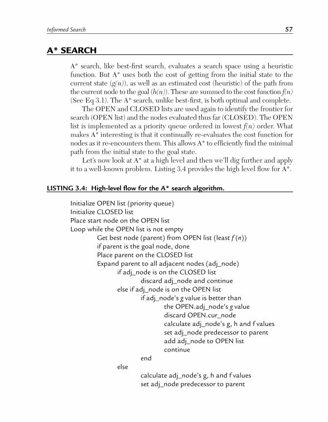
LISTING 3.4: High-level flow for the A* search algorithm.
Initialize OPEN list (priority queue)Initialize CLOSED listPlace start node on the OPEN listLoop while the OPEN list is not empty Get best node (parent) from OPEN list (least f (n)) if parent is the goal node, done Place parent on the CLOSED list Expand parent to all adjacent nodes (adj_node) if adj_node is on the CLOSED list discard adj_node and continue else if adj_node is on the OPEN list if adj_node’s g value is better than the OPEN.adj_node’s g value discard OPEN.cur_node calculate adj_node’s g, h and f values set adj_node predecessor to parent add adj_node to OPEN list continue end else calculate adj_node’s g, h and f values set adj_node predecessor to parent
58 Artificial Intelligence
add adj_node to OPEN list end endend loop
Note in the flow from Listing 3.4 that once we find the best node from the OPEN list, we expand all of the child nodes (legal states possible from the best node). If the new legal states are not found on either the OPEN or CLOSED lists, they are added as new nodes (setting the predecessor to the best node, or parent). If the new node is on the CLOSED list, we discard it and continue. Finally, if the new node is on the OPEN list, but the new node has a better g value, we discard the node on the OPEN list and add the new node to the OPEN list (otherwise, the new node is discarded, if its g value is worse). By re-evaluating the nodes on the OPEN list, and replacing them when cost functions permit, we allow better paths to emerge from the state space.
As we’ve defined already, A* is complete, as long as the memory supports the depth and branching factor of the tree. A* is also optimal, but this characteristic depends on the use of an admissible heuristic. Because A* must keep track of the nodes evaluated so far (and also the discovered nodes to be evaluated), the time and space complexity are both O(bd).
NOTE The heuristic is defined as admissible if it accurately estimates the path cost to the goal, or underestimates it (remains optimistic). This requires that the heuristic be monotonic, which means that the cost never decreases over the path, and instead monotonically increases. This means that g(n) (path cost from the initial node to the current node) monotonically increases, while h(n) (path cost from the current node to the goal node) monotonically decreases.
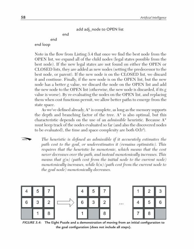
FIGURE 3.4: The Eight Puzzle and a demonstration of moving from an initial configuration to the goal configuration (does not include all steps).
Informed Search 59
A* Search and the Eight PuzzleWhile A* has been applied successfully to problem domains such as path-finding, we’ll apply it here to what’s called the Eight Puzzle (also known as the N by M, or n2-1 tile puzzle). This particular variation of the puzzle consists of eight tiles in a 3 by 3 grid. One location contains no tile, which can be used to move other tiles to migrate from one configuration to another (see Figure 3.4).
Note in Figure 3.4 that there are two legal moves that are possible. The ‘1’ tile can move left, and the ‘6’ tile can move down. The final goal configuration is shown at the right. Note that this is one variation of the goal, and the one that we’ll use here.
The Eight Puzzle is interesting because it’s a difficult problem to solve, but one that’s been studied at length and is therefore very well understood. [Archer 1999] For example, the number of possible board configurations of the Eight Puzzle is (n*n)!, but only half of these are legal configurations.
TIP During the 1870s, the Fifteen Puzzle (4 by 4 variant of the N by M puzzle) became a puzzle craze much like the Rubik’s cube of the 1970s and 1980s.
On average, 22 moves are required to solve the 3 by 3 variant of the puzzle. But considering 22 as the average depth of the tree, with an average branching factor of 2.67, 2.4 trillion non-unique tile configurations can be evaluated.
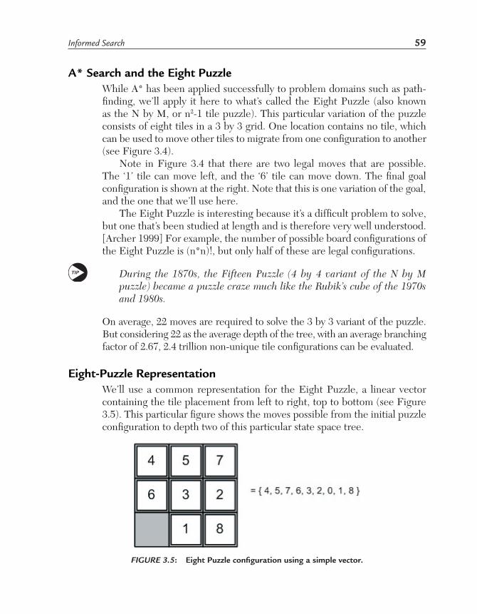
Eight-Puzzle RepresentationWe’ll use a common representation for the Eight Puzzle, a linear vector containing the tile placement from left to right, top to bottom (see Figure 3.5). This particular figure shows the moves possible from the initial puzzle configuration to depth two of this particular state space tree.
FIGURE 3.5: Eight Puzzle configuration using a simple vector.

60 Artificial Intelligence
For our heuristic, we’ll use the depth of the tree as the cost from the root to the current node (otherwise known as g(n)), and the number of misplaced tiles (h(n)) as the estimated cost to the goal node (excluding the blank). The path cost (f(n)) then becomes the cost of the path to the current node (g(n)) plus the estimated cost to the goal node (h(n)). You can see these heuristics in the tree in Figure 3.6. From the root node, only two moves are possible, but from these two moves, three new moves (states) open up. At the bottom of this tree, you can see that the cost function has decreased, indicating that these board configurations are likely candidates to explore next.
NOTE There are two popular heuristics for the N-puzzle problem. The first is simply the number of tiles out of place, which in general decreases as the goal is approached. The other heuristic is the Manhattan distance of
FIGURE 3.6: Eight Puzzle tree ending at depth two, illustrating the cost functions.

Informed Search 61
tiles which sums the tile distance of each out of place tile to its correct location. For this implementation, we’ll demonstrate the simple, but effective, tiles-out-of-place heuristic.
TIP While there are (3*3)! board configurations possible, there are only (3*3)!/2 valid configurations. The other half of the configurations are unsolvable. We’ll not dwell on this here, but in the source implementation you’ll see the test in initPuzzle using the concept of inversions to validate the configuration of the board. This concept can be further explored in [KGong 2005].
A* Search ImplementationThe core the of A-star algorithm is implemented in the function astar(). This function implements A-star as shown in Listing 3.4. We’ll also present the evaluation function, which implements the ‘tiles-out-of-place’ metric. The list and other support functions are not presented here, but are available on the CD-ROM for review.
NOTE The A* implementation can be found on the CD-ROM at ./software/ch3/astar.c.
Let’s start with the evaluation function which calculates the estimated cost from the current node to the goal (as the number of tiles out of place), see Listing 3.6. The function simply enumerates the 3 by 3 board as a one-dimensional vector, incrementing a score value whenever a tile is present in a position it should not be in. This score is then returned to the caller.
LISTING 3.6: The Eight Puzzle h(n) estimated cost metric.
double evaluateBoard( board_t *board_p ){ int i; const int test[MAX_BOARD-1]={1, 2, 3, 4, 5, 6, 7, 8 }; int score=0; for (i = 0 ; i < MAX_BOARD-1 ; i++) { score += (board_p->array[i] != test[i]); } return (double)score;}

62 Artificial Intelligence
The astar function is shown in Listing 3.7. Prior to calling this function, we’ve selected a random board configuration and placed it onto the OPEN list. We then work through the OPEN list, retrieving the best node (with the least f value using getListBest) and immediately place it on the CLOSED list. We check to see if this node is the solution, and if so, we emit the path from the initial node to the goal (which illustrates the moves that were made). To minimize searching too deeply in the tree, we halt enumerating nodes past a given depth (we search them no further).
The next step is to enumerate the possible moves from this state, which will be a maximum of four. The getChildBoard function is used to return an adjacent node (using the index passed in to determine which possible move to make). If a move isn’t possible, then a NULL is returned and it’s ignored.
With a new child node, we first check to see if it’s already been evaluated (if it’s on the CLOSED list). If it is, then we’re to destroy this node and continue (to get the child node for the current board configuration). If we’ve not seen this particular board configuration before, we calculate the heuristics for the node. First, we initialize the node’s depth in the tree as the parent’s depth plus one. Next, we call evaluateBoard to get the tiles-out-of-place metric, which will act as our h value (cost from the root node to this node). The g value is set to the current depth, and the f value is initialized with Eq 3.1.
(Eq 3.1)
We include an alpha and beta parameter here to give different weights to the g and h values. In this implementation, alpha is 1.0 and beta is 2.0. This means that more weight is given to the h value, and subsequently the closer a node is to the goal is weighed higher than its depth in the state space tree.
With the f value calculated, we check to see if the node is on the OPEN list. If it is, we compare their f values. If the node on the OPEN list has a worse f value, the node on the OPEN list is discarded and the new child node takes its place (setting the predecessor link to the parent, so we know how we got to this node). If the node on the OPEN list has a better f value, then the node on the OPEN list remains on the open list and the new child is discarded.
Finally, if the new child node exists on neither the CLOSED or OPEN list, it’s a new node that we’ve yet to see. It’s simply added to the OPEN list, and the process continues.
This algorithm continues until either one of two events occur. If the OPEN list becomes empty, then no solution was found and the algorithm

Informed Search 63
exits. If the solution is found, then showSolution is called, and the nodes linked together via the predecessor links are enumerated to show the solution from the initial node to the goal node.
LISTING 3.7: The A* algorithm.
void astar( void ){ board_t *cur_board_p, *child_p, *temp; int i; /* While items are on the open list */ while ( listCount(&openList_p) ) { /* Get the current best board on the open list */ cur_board_p = getListBest( &openList_p ); putList( &closedList_p, cur_board_p ); /* Do we have a solution? */ if (cur_board_p->h == (double)0.0) { showSolution( cur_board_p ); return; } else { /* Heuristic - average number of steps is 22 for a 3x3, so * don’t go too deep. */ if (cur_board_p->depth > MAX_DEPTH) continue; /* Enumerate adjacent states */ for (i = 0 ; i < 4 ; i++) { child_p = getChildBoard( cur_board_p, i ); if (child_p != (board_t *)0) { if ( onList(&closedList_p, child_p->array, NULL) ) { nodeFree( child_p ); continue; } child_p->depth = cur_board_p->depth + 1; child_p->h = evaluateBoard( child_p ); child_p->g = (double)child_p->depth; child_p->f = (child_p->g * ALPHA) + (child_p->h * BETA); /* New child board on the open list? */ if ( onList(&openList_p, child_p->array, NULL) ) { temp = getList(&openList_p, child_p->array); if (temp->g < child_p->g) {

64 Artificial Intelligence
nodeFree(child_p); putList(&openList_p, temp); continue; } nodeFree( temp ); } else { /* Child board either doesn’t exist, or is better than a * previous board. Hook it to the parent and place on the * open list. */ child_p->pred = cur_board_p; putList( &openList_p, child_p ); } } } } } return;}
Eight Puzzle Demonstration with A*In the implementation, the tiles are labeled A-H with a space used to denote the blank tile. Upon execution, once the solution is found, the path taken from the initial board to the goal is enumerated. This is shown below in Listing 3.8, minimized for space.
LISTING 3.8: A sample run of the A* program to solve the Eight Puzzle.
$./astarGBDFCH EABGDFCHE ABGDFCHEAGBDFC

Informed Search 65
EAH...ABC DFGEHABCD FGEHABCDEFG HABCDEFGH
A* VariantsThe popularity of A* has spawned a number of variants that offer different characteristics. The Iterative-Deepening A* algorithm backtracks to other nodes when the cost of the current branch exceeds a threshold. To minimize the memory requirements of A*, the Simplified Memory-Bounded A* algorithm (SMA*) was created. SMA* uses the memory made available to it, and when it runs out of memory, the algorithm drops the least promising node to make room for new search nodes from the frontier.
Applications of A* SearchA* search is a popular technique and has seen use as a path-finding algorithm for computer strategy games. For better performance, many games employ simpler shortcut methods for path-finding by limiting the space of their movement (using a much sparser graph over the landscape), or by pre-calculating routes for in-game use.
HILL-CLIMBING SEARCH
Hill climbing is an iterative improvement algorithm that is similar to greedy best-first search, except that backtracking is not permitted. At each step in the search, a single node is chosen to follow. The criterion for the node to follow is that it’s the best state for the current state. Since the frontier for the search is a single node, the algorithm is also similar to beam search using a beam width of one (our OPEN list can contain exactly one node).

66 Artificial Intelligence
The problem with hill climbing is that the best node to enumerate locally may not be the best node globally. For this reason, hill climbing can lead to local optimums, but not necessarily the global optimum (the best solution available). Consider the function in Figure 3.7. There exists a local optimum and a global optimum. The goal should be to maximize the function, but if we begin at the far left and work our way toward the global optimum, we get stuck at the local optimum.
SIMULATED ANNEALING (SA)
Simulated Annealing (SA) is another iterative improvement algorithm in which randomness is incorporated to expand the search space and avoid becoming trapped in local minimum. As the name implies, the algorithm simulates the process of annealing.
Annealing is a technique in metal-casting where molten metal is heated and then cooled in a gradual manner to evenly distribute the molecules into a crystalline structure. If the metal is cooled too quickly, a crystalline structure does not result, and the metal solid is weak and brittle (having been filled with bubbles and cracks). If cooled in a gradual and controlled way, a crystalline structure forms at a molecular level resulting in great structural integrity.
The basic algorithm for simulated annealing is shown in Listing 3.9. We start with an initial solution candidate and the loop while the temperature is greater than zero. In this loop, we create an adjacent candidate solution by perturbing our current solution. This changes the solution to a neighboring solution, but at random. We then calculate the delta energy between the new (adjacent) solution, and our current solution. If this delta energy is less
FIGURE 3.7: State space illustrating the problem with hill climbing.
Informed Search 67
than zero, then our new solution is better than the old, and we accept it (we move the new adjacent solution to our current solution).
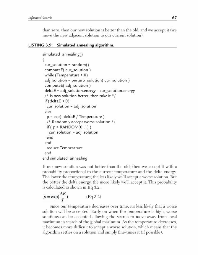
LISTING 3.9: Simulated annealing algorithm.
simulated_annealing(){ cur_solution = random() computeE( cur_solution ) while (Temperature > 0) adj_solution = perturb_solution( cur_solution ) computeE( adj_solution ) deltaE = adj_solution.energy – cur_solution.energy /* Is new solution better, then take it */ if (deltaE < 0) cur_solution = adj_solution else p = exp( -deltaE / Temperature ) /* Randomly accept worse solution */ if ( p > RANDOM(0..1) ) cur_solution = adj_solution end end reduce Temperature endend simulated_annealing
If our new solution was not better than the old, then we accept it with a probability proportional to the current temperature and the delta energy. The lower the temperature, the less likely we’ll accept a worse solution. But the better the delta energy, the more likely we’ll accept it. This probability is calculated as shown in Eq 3.2.
(Eq 3.2)
Since our temperature decreases over time, it’s less likely that a worse solution will be accepted. Early on when the temperature is high, worse solutions can be accepted allowing the search to move away from local maximum in search of the global maximum. As the temperature decreases, it becomes more difficult to accept a worse solution, which means that the algorithm settles on a solution and simply fine-tunes it (if possible).

68 Artificial Intelligence
The classical simulated annealing algorithm also includes monte carlo cycles where a number of trials are performed before decreasing the temperature.
The Traveling Salesman Problem (TSP)To demonstrate the simulated annealing algorithm, we’ll use the classic Traveling Salesman Problem (or TSP). In the TSP, we’re given a set of cities and a relative cost for traveling between each city to each other. The goal is to find a path through all cities where we visit all cities once, and find the shortest overall tour. We’ll start at one city, visit each other city, and then end at the initial city.
Consider the graph shown in Figure 3.8. Many cities are connected to one another, but an optimal path exists that tours each city only once.
The TSP is both interesting and important because it has practical implications. Consider transportation problems where deliveries are required and fuel and time are to be minimized. Another interesting application is that of drilling holes in a circuit board. A number of holes must be drilled quickly on a single board, and in order to do this, an optimal path is needed to minimize the movement of the drill (which will be slow). Solutions to the TSP can therefore be very useful.
TSP Tour RepresentationTo represent a set of cities and the tour between them, we’ll use an implicit adjacency list. Each city will be contained in the list, and cities that are next to one another are implied as connected in the tour. Recall our sample TSP in Figure 3.8 where seven cities make up the world. This will be represented as shown in Figure 3.9.
FIGURE 3.8: A Sample TSP tour through a small graph.

Informed Search 69
FIGURE 3.9: Adjacency list for the TSP tour shown in Figure 3.8.
FIGURE 3.10: Demonstration of row swapping to perturb the tour.

70 Artificial Intelligence
Note that the list shown in Figure 3.9 is a single list in tour order. When we reach the end of the list, we wrap to the first element, completing the tour. To perturb the tour we take two random rows from the list and swap them. This is demonstrated in Figure 3.10. Note how by simply swapping two elements, the tour is greatly perturbed and results in a worse tour length.
Simulated Annealing ImplementationThe implementation of simulated annealing is actually quite simple in the C language. We’ll review three of the functions that make up the simulated annealing implementation, the main simulated annealing algorithm, perturbing a tour, and computing the length of the tour. The remaining functions are available on the CD-ROM.
LISTING 3.10: Structures for the TSP solution.
typedef struct { int x, y;} city_t;typedef struct {city_t cities[MAX_CITIES];double tour_length;} solution_t;
The Euclidean distance of the tour is calculated with compute_tour. This function walks through the tour, accumulating the segments between each city (see Listing 3.11). It ends by wrapping around the list, and adding in the distance from the last city back to the first.
LISTING 3.11: Calculating the Euclidean tour with compute_tour.
void compute_tour( solution_t *sol ){ int i; double tour_length = (double)0.0; for (i = 0 ; i < MAX_CITIES-1 ; i++) { tour_length += euclidean_distance( sol->cities[i].x, sol->cities[i].y, sol->cities[i+1].x, sol->cities[i+1].y );
Informed Search 71
}tour_length += euclidean_distance( sol->cities[MAX_CITIES-1].x, sol->cities[MAX_CITIES-1].y, sol->cities[0].x, sol->cities[0].y ); sol->tour_length = tour_length; return;}
Given a solution, we can create an adjacent solution using the function perturb_tour. In this function, we randomly select two cities in the tour, and swap them. A loop exists to ensure that we’ve selected two unique random points (so that we don’t swap a single city with itself). Once selected, the x and y coordinates are swapped and the function is complete.
LISTING 3.12: Perturbing the tour by creating an adjacent solution.
void perturb_tour( solution_t *sol ){ int p1, p2, x, y; do { p1 = RANDMAX(MAX_CITIES); p2 = RANDMAX(MAX_CITIES); } while (p1 == p2); x = sol->cities[p1].x; y = sol->cities[p1].y; sol->cities[p1].x = sol->cities[p2].x; sol->cities[p1].y = sol->cities[p2].y; sol->cities[p2].x = x; sol->cities[p2].y = y; return;}
Finally, the simulated_annealing function implements the core of the simulated annealing algorithm. The algorithm loops around the temperature, constantly reducing until it reaches a value near zero. The initial solution has been initialized prior to this function. We take the current solution and perturb it (randomly alter it) for a number of

72 Artificial Intelligence
iterations (the Monte Carlo step). If the new solution is better, we accept it by copying it into the current solution. If the new solution is worse, then we accept it with a probability defined by Eq 3.2. The worse the new solution and the lower the temperature, the less likely we are to accept the new solution. When the Monte Carlo step is complete, the temperature is reduced and the process continues. When the algorithm completes, we emit the city tour.
LISTING 3.13: The simulated annealing main function implementation.
int simulated_annealing( void ){ double temperature = INITIAL_TEMP, delta_e; solution_t tempSolution; int iteration; while( temperature > 0.0001 ) { /* Copy the current solution to a temp */ memcpy( (char *)&tempSolution, (char *)&curSolution, sizeof(solution_t) ); /* Monte Carlo Iterations */ for (iteration = 0 ; iteration < NUM_ITERATIONS ; iteration++) { perturb_tour( &tempSolution ); compute_tour( &tempSolution ); delta_e = tempSolution.tour_length – curSolution.tour_length; /* Is the new solution better than the old? */ if (delta_e < 0.0) { /* Accept the new, better, solution */ memcpy( (char *)&curSolution, (char *)&tempSolution, sizeof(solution_t) ); } else { /* Probabilistically accept a worse solution */ if ( exp( (-delta_e / temperature) ) > RANDOM()) { memcpy( (char *)&curSolution, (char *)&tempSolution, sizeof(solution_t) ); } } } /* Decrease the temperature */

Informed Search 73
temperature *= ALPHA; } return 0;}
Simulated annealing permits a random walk through a state space, greedily following the best path. But simulated annealing also probabilistically allows following worse paths in an effort to escape local maximums in search of the global maximum. This makes simulated annealing a random search, but heuristically driven. For all of its advantages, simulated annealing is incomplete and suboptimal.
Simulated Annealing DemonstrationLet’s now look at the simulated annealing algorithm in action. We’ll look at the algorithm from a variety of perspectives, from the temperature schedule, to a sample solution to TSP for 25 cities.
FIGURE 3.11: The temperature decay curve using Eq 3.3.
74 Artificial Intelligence
The temperature schedule is a factor in the probability for accepting a worse solution. In this implementation, we’ll use a geometric decay for the temperature, as shown in Eq 3.3.
T = aT (Eq 3.3)In this case, we use an alpha of 0.999. The temperature decay using this
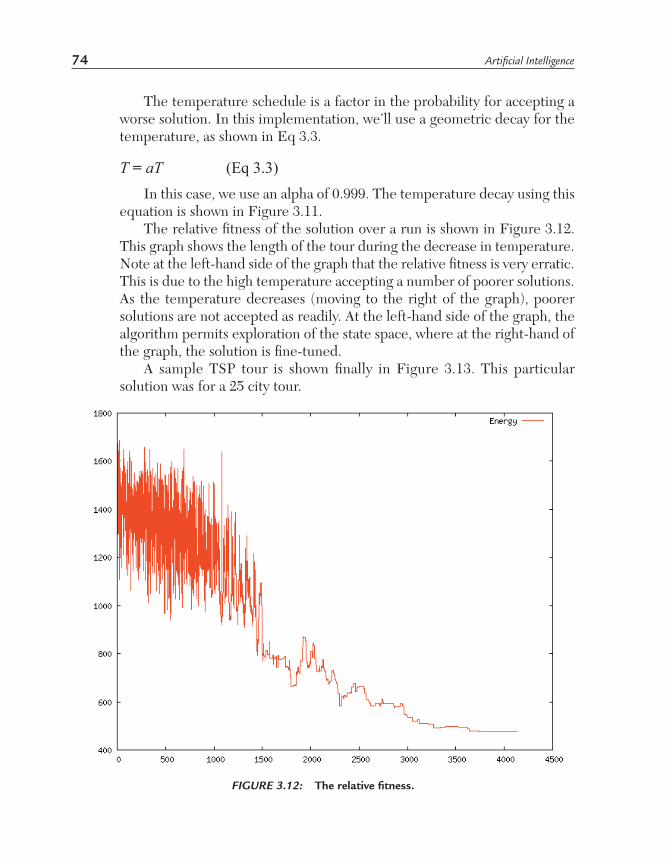
equation is shown in Figure 3.11.The relative fitness of the solution over a run is shown in Figure 3.12.
This graph shows the length of the tour during the decrease in temperature. Note at the left-hand side of the graph that the relative fitness is very erratic. This is due to the high temperature accepting a number of poorer solutions. As the temperature decreases (moving to the right of the graph), poorer solutions are not accepted as readily. At the left-hand side of the graph, the algorithm permits exploration of the state space, where at the right-hand of the graph, the solution is fine-tuned.
A sample TSP tour is shown finally in Figure 3.13. This particular solution was for a 25 city tour.
FIGURE 3.12: The relative fitness.

Informed Search 75
TABU SEARCH
Tabu search is a very simple search algorithm that is easy to implement and can be very effective. The basic idea behind Tabu search is neighborhood search with a Tabu list of nodes that is made up of nodes previously evaluated. Therefore, the search may deteriorate, but this allows the algorithm to widen the search to avoid becoming stuck in local maxima. During each iteration of the algorithm, the current search candidate is compared against the best solution found so far so that the best node is saved for later. After some search criteria has been met (a solution found, or a maximum number of iterations) the algorithm exits.
The Tabu list can be of finite size so that the oldest nodes can be dropped making room for new Tabu nodes. The nodes on the Tabu list can also be timed, such that a node can only be Tabu for some period of time. Either case allows the algorithm to reuse the Tabu list and minimize the amount of memory needed.
FIGURE 3.13: Sample TSP tour optimized by simulated annealing.

76 Artificial Intelligence
Monitoring Tabu search through the state space of the 4-Queens problem is shown in Figure 3.14. The initial position is the root, which has a score of three (three conflicts). The goal is to minimize the score, where zero is a solution (goal node). At the first iteration, the neighbor nodes are evaluated, and the best selected. Note also here that our initial node has been placed on the Tabu list. At iteration two, the neighbors are evaluated for the current node and the best is chosen to move forward. The Tabu list now contains the previous two best nodes. In this iteration, we’ve found a node with a score of zero, which indicates a goal node and the algorithm terminates.
The basic flow for Tabu search is shown in Listing 3.14. Given an initial position (shown here as a initial random position), the search space is enumerated by taking the best neighbor node that is not Tabu. If it’s better than our best saved solution, it becomes the best solution. The process then continues with the last solution until a termination criteria is met.
FIGURE 3.14: The 4-Queens problem solved by Tabu search.

Informed Search 77
LISTING 3.14: The basic flow of the Tabu search algorithm.
tabu_search(){cur_solution = random()evaluate_position( cur_solution )best = cur_solution tabu( cur_solution ) while (!termination_critera) {
/* Get the best neighbor, not on the tabu list */ cur_solution = best_non_tabu_neighbor( cur_solution ) evaluate_position( cur_solution )
tabu( cur_solution ) if (cur_solution.f < best.f) { best = cur_solution }} return best}
To illustrate the Tabu search algorithm, we’ll use the N-Queens problem as demonstrated with the best-first search algorithm. (See Figure 3.1 for a recap of the problem and desired solution.) After discussing the basic Tabu search implementation, we’ll explore some of the variants that improve the algorithm.
Tabu Search ImplementationThe Tabu search algorithm is very simple and can be illustrated in a single function (see Listing 3.15, function tabu_s). This function is the core of the Tabu search algorithm. The supporting functions are not shown here, but are available on the CD-ROM.
O
N THE CD
The C source language implementation of Tabu search can be found on the CD-ROM at ./software/ch3/tabus.c.
The implementation begins with a seeding of the random function (RANDINIT) followed by the creation of the Tabu queue. This queue represents our Tabu list, or those elements that will not be evaluated further

78 Artificial Intelligence
if rediscovered. The initial solution is then created, and copied to the best solution (via initBoard to create the solution, and evaluateBoard to evaluate the value of the solution). The current solution is then loaded onto the Tabu list so that it’s not evaluated again.
The loop then begins, for which we’ll operate forever, or until a solution is found. For this simple problem, we’ll always find a solution in some number of iterations. The call to reviewChildNodes evaluates the neighbor solutions, and picks the best one that is not on the Tabu list. This solution is returned (by reference) and then loaded onto the Tabu list. Note here that we first check to see if it’s already on the Tabu list. If not, we check the state of the Tabu list. If full, we need the oldest element to make room for the new node, and then add it to the queue.
TIP Recall that queues are FIFO in nature. Therefore, removing a node from the queue automatically removes the oldest node, satisfying the policy for the algorithm (remove the oldest node first, if the Tabu list is full).
Finally, we check the value of the solution, and if zero, we have the goal node. This can now be emitted using the emitBoard function.
LISTING 3.15: Basic Tabu search algorithm implementation in C.
void tabu_s(){ unsigned short best_sol, cur_sol; int best_f, cur_f; RANDINIT(); tabu_q = createQueue(MAX_ELEMENTS); /* Get initial board */ cur_sol = best_sol = initBoard(); cur_f = best_f = evaluateBoard( best_sol ); enQueue( tabu_q, best_sol ); while( 1 ) { printf(“Iteration for %x\n”, cur_sol); /* Return (by reference) the best non-tabu neighbor */ reviewChildNodes( &cur_sol, &cur_f ); /* Add the current best solution to the tabu list (remove * the oldest if needed). */ if (!searchQueue( tabu_q, cur_sol )) { if (isFullQueue( tabu_q )) {

Informed Search 79
(void)deQueue( tabu_q ); } enQueue( tabu_q, cur_sol ); } /* Save the best solution so far */ if (cur_f <= best_f) { best_sol = cur_sol; best_f = cur_f; } /* Solution found? */ if (best_f == 0 ) { emitBoard( best_sol ); break; } } destroyQueue( tabu_q ); return;}
Tabu Search DemonstrationThe Tabu search application efficiently finds the solution to this problem (a state space of 256 unique nodes). The first evaluateBoard is the initial node (see Listing 3.16), followed by four iterations of the algorithm. Note that while the initial node had a cost of two, subsequent nodes evaluated were worse, but eventually led to the goal. Tabu search permits the evaluation away from local minimum to find the global minimum, as demonstrated here.
LISTING 3.16: Sample execution of Tabu search for the 4-Queens problem.
evaluateBoard 1281 = (f 2)Iteration for 1281 evaluateBoard 2281 = (f 2) evaluateBoard 2181 = (f 3) evaluateBoard 2481 = (f 3) evaluateBoard 2241 = (f 2) evaluateBoard 2221 = (f 3) evaluateBoard 2281 = (f 2) evaluateBoard 2282 = (f 3)Iteration for 2281 evaluateBoard 4281 = (f 1)

80 Artificial Intelligence
evaluateBoard 4181 = (f 1) evaluateBoard 4481 = (f 3) evaluateBoard 4281 = (f 1) evaluateBoard 4241 = (f 3) evaluateBoard 4282 = (f 2)Iteration for 4281 evaluateBoard 8281 = (f 2) evaluateBoard 8181 = (f 3) evaluateBoard 8481 = (f 4) evaluateBoard 8241 = (f 2) evaluateBoard 8221 = (f 3) evaluateBoard 8281 = (f 2) evaluateBoard 8282 = (f 2)Iteration for 8282 evaluateBoard 4282 = (f 2) evaluateBoard 2282 = (f 3) evaluateBoard 4182 = (f 0) evaluateBoard 4482 = (f 2) evaluateBoard 4282 = (f 2) evaluateBoard 4142 = (f 2) evaluateBoard 4181 = (f 1) evaluateBoard 4184 = (f 3)solution is 0x41820 1 0 0 0 0 0 1 1 0 0 0 0 0 1 0
Tabu Search VariantsIn order to make Tabu search more effective for very difficult search problems, a number of modifications exist. The first of these is called intensification and essentially intensifies the search around a given point (such as the best known solution). The idea is that we take a promising node, and intensify the search around this point. This is implemented using an intermediate memory, which contains the neighbor nodes to dig into further.
One issue that comes up in local search algorithms is that they can get stuck in local optimums. Tabu search introduces the concept of diversification to allow the algorithm to search nodes that have been previously unexplored to expand the space of search.

Informed Search 81
When we follow the best solutions, it’s very possible to get stuck in local optimums for difficult problems. Another interesting variant is called constraint relaxation, which relaxes the neighborhood selection algorithm to accept lower quality nodes in the search space. This permits the algorithm to expand its search to descend into lower quality solutions in search of higher quality solutions. [Gendreau 2002]
CONSTRAINT SATISFACTION PROBLEMS (CSP)
In many search problems, we’re interested not just in the goal, but how we got from the initial state to the goal state (take for example, the eight puzzle). As we’ll learn later, planning systems rely on this aspect of search as a plan is nothing more than a sequence of steps to get from a given state to a goal state. For some problems, we’re not interested in the path to the goal, but instead just the goal state (for example, the N-Queens problem). Problems of this type are called Constraint Satisfaction Problems (CSP).
Formally, we can think about CSP in terms of a set of variables with a domain of possible values, and a set of constraints that specify the allowable combinations of variable values. Consider the following simple example. We wish to find values for the set of variables x and y each having a domain of {1-9}, such that Eq 3.4 (the constraint) is satisfied.
x + y = x * y (Eq 3.4)
Without much work, we know that assigning the value of two for both x and y satisfies the constraint defined by the equation.
Graph Coloring as a CSPOne of the more popular CSPs is called Graph Coloring. Given a graph, and a set of colors, the problem is to color the nodes such that an edge does not directly connect to a node of the same color. Consider the map shown in Figure 3.15. We can see a set of objects that are adjacent to one another. Object A is adjacent to objects B and C, while object D is adjacent only to object B. The graph portion of Figure 3.14 illustrates the graph of the map. From this graph, we can see edges which define the adjacency of the objects (nodes) of the graph.
Now consider the problem of coloring the map given the constraints that each object can be one color and no colored objects should be adjacent to one another. Can the graph be colored using three colors (red, green, and blue)?

82 Artificial Intelligence
Using trial and error, we can very easily color this simple graph by iterating through the nodes of the graph and assigning a color so that our constraint remains satisfied. Let’s start with node A, color it, and then step to each remaining node, coloring as we go. In Listing 3.17, we see the coloring process. Each node is followed by a constraint, with the color finally chosen in parentheses. Node A – Pick any color (Red) Node B – Pick a color other than Red (Blue) Node C – Pick a color other than Red and Blue (Green) Node D – Pick a color other than Blue (Red) Node E – Pick a color other than Green (Red) Node F – Pick a color other than Green or Red (Blue) Node G – Pick a color other than Red or Blue (Green)
LISTING 3.17: Graph coloring through trial and error.
Through a simple process of elimination, we’ve been able to color the graph using the constraints of previously colored nodes to determine the color to paint adjacent nodes (final result shown in Figure 3.17).
FIGURE 3.15: The classical graph coloring CSP.

Informed Search 83
TIP The famous Four Color Theorem (to prove that only four colors are required to color any planar map) dates back to the mid 1800s. There were numerous failed attempts to prove the theorem and it remained conjecture until 1976, when Appel and Haken created a formal proof.
Scheduling as a CSPOne of the most practical applications of constraint satisfaction is to the problem of scheduling. Numerous types of scheduling problems exist, from airline timetables to the scheduling of manufacturing processes. The scheduling problem comes down to allocating resources to activities in time preserving a set of constraints. For example, in a manufacturing problem, a resource can be processed through a variety of activities each requiring a specific amount of time. In addition, activities have precedence that must be maintained (a resource must be processed by Activity A before Activity B). The goal of the CSP in this problem is to identify an optimal schedule of resources through the activities such that the end product can be optimally produced.
FIGURE 3.16: Result of Graph Coloring from Listing 3.17.

84 Artificial Intelligence
CONSTRAINT-SATISFACTION ALGORITHMSA large number of algorithms exist to solve CSPs from the simple Generate and Test algorithm to constraint-propagation and consistency. We’ll explore a few of the available algorithms that can be used. Note that some of the algorithms we’ve discussed thus far (such as depth-first search investigated in Chapter 2, and simulated annealing and Tabu search from Chapter 3) can be used effectively to solve CSPs.
Generate and TestGenerate and Test is the simplest of the algorithms to identify a solution for a CSP. In this algorithm, each of the possible solutions is attempted (each value enumerated for each variable) and then tested for the solution. Since testing each combination of variable within the domain of each value can be extremely slow and inefficient, heuristics can be applied to avoid those combinations that are outside of the solution space.
BacktrackingThe backtracking algorithm operates with a simple uninformed search algorithm, such as depth-first search. At each node, a variable is instantiated with a value and the constraint violations are checked. If the values are legal, search is permitted to continue, otherwise, the current branch is abandoned and the next node from the OPEN list is evaluated.
To increase the efficiency of the backtracking algorithm, the most constrained variable is instantiated first. Take for example, node C from Figure 3.14. In this case, the node has four neighbors (the most of any node in the graph).
TIP Both Generate and Test and backtracking are common systematic search algorithms, as they systematically assign values to variables in search of a solution. Generate and Test is highly inefficient, while backtracking suffers from trashing, or the repeated failure to find a solution for the same reason (for example, a single variable remaining constant).
Forward Checking and Look AheadForward checking is similar to backtracking, except that when a particular node is evaluated for the current variable (called arc consistency), only those valid nodes are considered for the OPEN list to evaluate in the future. Nodes that can be detected as invalid are immediately ignored, resulting only in the

Informed Search 85
most promising branches for further search. This can minimize a number of nodes generated for search, but tends to involve more work when evaluating a single node (for forward checking of constraints).
A variation on forward checking is called look ahead. In this algorithm, instead of simply evaluating child nodes based on the currently instantiated value, all subsequent to be instantiated variables are instantiated given the currently instantiated values. This results in very flat search trees. (See Figure 3.17 for a graphical view of backtracking, forward checking, and look ahead.)
TIP Forward checking is commonly more effective than backtracking as the number of nodes to be evaluated is reduced.
FIGURE 3.17: Comparison of backtracking, forward checking, and look ahead constraint propagation algorithms.

86 Artificial Intelligence
Min-Conflicts SearchAn interesting heuristic repair algorithm is the Min-Conflicts heuristic. This algorithm begins by choosing the variable that violates the fewest number of constraints and then systematically improves the solution through using an algorithm such as hill climbing or A* with the heuristic function h(n) defined as the total number of constraints violated.
CHAPTER SUMMARYInformed search methods, unlike the uninformed (or blind) methods, use a heuristic to determine the quality of any state in the search space. This allows the algorithm to guide the search and choose the next node to expand. In this chapter, a number of informed search methods were explored, including best-first search, A* search, hill-climbing search, simulated annealing, Tabu search, and finally algorithms for constraint satisfaction. Understanding the informed methods of search is important because much of problem solving in AI can be refined to search methods. The key is choosing the algorithm that is best suited to the particular problem at hand.
ALGORITHMS SUMMARY
Table 3.1: Summary of the uninformed algorithms and their characteristics.
Algorithm Time Space Optimal Complete DerivativeBest-First Search O(bm) O(bm) No Yes BFS/UCSA* Search O(2N) O(bd) Yes Yes BestFSIDA* O(2N) O(d) Yes Yes A*SMA*SimAnneal - - No NoTabu - - No Nob, branching factord, tree depth of the solutionm, tree depth
REFERENCES[Archer 1999] Archer, A.F. “A Modern Treatment of the 15 Puzzle,”
American Math. Monthly 106, 793-799, 1999.

Informed Search 87
[KGong 2005] Gong, Kevin. “A Mathematical Analysis of the Sixteen Puzzle.” Last updated 12/2005.
Available online at http://www.kevingong.com/Math/SixteenPuzzle.html[Gendreau 2002] Gendreau, Michel. “An Introduction to Tabu Search,”
Universite de Montreal. July 2002. Available online at http://www.ifi.uio.no/infheur/Bakgrunn/Intro_to_TS_Gendreau.htm
RESOURCES
[Glover 1990] Glover, Fred. “Tabu Search: A Tutorial,” Interfaces, 20 (4): 74-94, 1990.
EXERCISES
1. Best-first search uses a combined heuristic to choose the best path to follow in the state space. Define the two heuristics used (h(n) and g(n)).
2. Best-first search uses both an OPEN list and a CLOSED list. Describe the purpose of each for the best-first algorithm.
3. Describe the differences between best-first search and greedy best-first search.
4. Describe the differences between best-first search and beam search.5. What are the advantages of beam search over best-first search?6. A* search uses a combined heurstic to select the best path to follow
through the state space toward the goal. Define the two heuristics used (h(n) and g(n)).
7. Briefly describe A* search and the problems to which it can be applied.
8. What is meant by an admissible heuristic?9. How do the alpha and beta parameters tune the heuristics for A*
search?10. Briefly explain the difference between A* search and SMA*. What
advantage does SMA have over A*?11. Hill climbing is a standard iterative improvement algorithm similar
to greedy best-first search. What are the primary problems with hill climbing?
12. Describe Simulated annealing and if it combines iterative improvement with stochastic search.
13. Describe the algorithm and how it differs from random search.

88 Artificial Intelligence
14. What is the purpose of the Monte Carlo step in the simulated annealing algorithm?
15. Briefly describe the Tabu search algorithm.16. The Tabu list can be sized for the problem at hand. What effect does
changing the size of the Tabu list have on the search algorithm?17. Describe the intensification and diversification modifications of Tabu
search.18. Describe the essence of a constraint satisfaction problem.19. What are some of the major applications of constraint satisfaction
search?20. Compare and contrast the CSP algorithms of backtracking, forward
checking, and look ahead.

C h a p t e r
AI has a long history in the genre of games. From the first intelligent Checkers player, to the team AI developed for first-person-shooters, AI is at the core. This chapter will cover aspects of game AI from
traditional game playing of Checkers, Chess, Othello, and Go to more recent video games including first-person-shooters, strategy games, and others. We’ll introduce the minimax algorithm and alpha-beta pruning, which are central to traditional two-player games. We’ll then explore other algorithms that can be found in modern game systems.
TWO-PLAYER GAMES
Two-player games are games in which two players compete against each other. These are also known as zero-sum games. The goal then in playing a two-player game is choosing a move that maximizes the score of the player and/or minimizes the score of the competing player.
NOTE A zero-sum game is one in which the gain of one player is balanced exactly by the loss of the other player. Zero sum games have been studied extensively by John von Neumann and Oskar Morgenstern and then
4 AI AND GAMES

90 Artificial Intelligence
later by John Nash. Chess is an example of a zero-sum game. In contrast, non-zero-sum games are those in which two players attempt to get rewards from a banker by cooperating or betraying the other player. The prisoner’s dilemma is a classic example of a non-zero-sum game. Both zero and non-zero-sum games are types of games within the field of game theory. Game theory has a range of uses from parlor games such as Poker, to the study of economic phenomena from auctions to social networks.
Consider the two-player game Tic-Tac-Toe. Players alternate moves, and as each move is made, the possible moves are constrained (see the partial Tic-Tac-Toe game tree in Figure 4.1). In this simple game, a move can be selected based on the move leading to a win by traversing all moves that are constrained by this move. Also, by traversing the tree for a given move, we can choose the move that leads to the win in the shallowest depth (minimal number of moves).
Tic-Tac-Toe is an interesting case because the maximum number of moves is tiny when compared to more complex games such as Checkers or
FIGURE 4.1: Partial game tree for the two-player game of Tic-Tac-Toe.

AI and Games 91
Chess. Tic-Tac-Toe is also open to numerous optimizations. Consider, for example, the first X move in Figure 4.1. If the board is rotated, only three unique moves are actually possible. Without optimization, there exist 362,880 nodes within the complete game tree.
NOTE Two-player games are useful as a test-bed for validating competitive algorithms. Also of interest are one-player games (also known as puzzles). Examples of useful one-player games include the n-disk Towers of Hanoi puzzle and the N-puzzle (see Chapters 2 and 3).
At each node in the tree (a possible move) a value defining the goodness of the move toward the player winning the game can be provided. So at a given node, the child nodes (possible moves from this state in the game) each have an attribute defining the relative goodness of the move. It’s an easy task then to choose the best move given the current state. But given the alternating nature of two-player games, the next player makes a move that benefits himself (and in zero-sum games, results in a deficit for the alternate player).
A static evaluation function (that measure the goodness of a move) is used to determine the value of a given move from a given game state. The evaluation function identifies the relative value of a successor move from the list of possible moves as a measure of the move quality toward winning the game. Consider the partial game tree in Figure 4.2.
The static evaluation function is defined as the number of possible win positions not blocked by the opponent minus the number of possible win positions (row, column, and diagonal) for the opponent not blocked by the current player:
FIGURE 4.2: Tic-Tac-Toe game tree with static evaluation function.

92 Artificial Intelligence
f (n) = win_positions-lose_positions (Eq 4.1)
Using this evaluation function, we identify the goodness of the board configuration given a move for X in Figure 4.2. The higher the result of the static evaluation function, the closer the move brings the player toward a win. Three moves result in the evaluation function equaling three, but only one move can lead to a win for X as the other two lead to a subsequent win for O. Therefore, while the static evaluation function is useful, another heuristic is necessary to pick the move with the highest static evaluation while protecting against a loss in the next move.
Let’s now look at an algorithm that provides a means to select a move that brings the player closer to a win while moving the opponent further from a win.
THE MINIMAX ALGORITHM
In simple games, algorithms exist that can search the game trees to determine the best move to make from the current state. The most well known is called the Minimax algorithm. The minimax algorithm is a useful method for simple two-player games. It is a method for selecting the best move given an alternating game where each player opposes the other working toward a mutually exclusive goal. Each player knows the moves that are possible given a current game state, so for each move, all subsequent moves can be discovered.
At each node in the tree (possible move) a value defining the goodness of the move toward the player winning the game can be provided. So at a given node, the child nodes (possible moves from this state in the game) each have an attribute defining the relative goodness of the move. It’s an easy task then to choose the best move given the current state. But given the alternating nature of two-player games, the next player makes a move that benefits them (and in zero-sum games, results in a deficit for the alternate player).
NOTE The ply of a node is defined as the number of moves needed to reach the current state (game configuration). The ply of a game tree is then the maximum of the plies of all nodes.
Minimax can use one of two basic strategies. In the first, the entire game tree is searched to the leaf nodes (end-games), and in the second, the tree is searched only to a predefined depth and then evaluated. Let’s now explore the minimax algorithm in greater detail.

AI and Games 93
NOTE When we employ a strategy to restrict the search depth to a maximum number of nodes (do not search beyond N levels of the tree), the look ahead is restricted and we suffer from what is called the horizon effect. When we can’t see beyond the horizon, it becomes easier to make a move that looks good now, but leads to problems later as we move further into this subtree.
Minimax is a depth-first search algorithm that maintains a minimum or a maximum value for successor nodes at each node that has children. Upon reaching a leaf node (or the max depth supported), the value of the node is calculated using an evaluation (or utility) function. Upon calculating a node’s utility, we propagate these values up to the parent node based on whose move is to take place. For our move, we’ll use the maximum value as our determiner for the best move to make. For our opponent, the minimum value is used. At each layer of the tree, the child nodes area is scanned and depending on whose move is to come, the maximum value is kept (in the case of our move), or the minimum value is kept (in the case of the opponent’s move). Since these values are propagated up in an alternating fashion, we maximize the minimum, or minimize the maximum. In other words, we assume that each player makes the move next that benefits them the most. The basic algorithm for minimax is shown in Listing 4.1.
LISTING 4.1: Basic algorithm for minimax game tree search.
minimax( player, board ) if game_won( player, board ) return win for each successor board if (player == X) return maximum of successor boards if (player == O) return minimum of successor boards endend
To demonstrate this approach, Figure 4.3 shows the end-game for a particular Tic-Tac-Toe board configuration. Both X and O have played three turns, and now it’s X’s turn. We traverse this tree in depth-first order, and upon reaching either a win/lose or draw position, we set the score for the board. We’ll use a simple representation here, -1 representing a loss, 0 for a draw, and 1 for a win. The boards with bold lines define the win/loss/draw boards where the score is evaluated. When all leaf nodes have been evaluated, the node values can be propagated up based on the current player.

94 Artificial Intelligence
At layer 2 in the game tree, it’s O’s turn, so we minimize the children and score the parent with the smallest value. At the far left portion of the game tree, the values 0 and 1 are present, so 0 is kept (the minimum) and stored in the parent. At layer 1 in the tree, we’re looking at the maximum, so out of node scores 0, -1, and -1, we keep 0 and store this at the parent (the root node of our game tree).
With the scores having been propagated to the root, we can now make the best move possible. Since it’s our move, we’re maximizing, so we look for the node with the largest score (the left-most node with a value of 0), and we take this position. Our opponent (who is minimizing) then chooses the minimum node value (left-most node in tree depth 2). This leaves us with our final move, resulting in a draw.
Note that in a game where perfect information is available to each player, and no mistakes are made, the end-result will always be a draw. We’ll build a program to play Tic-Tac-Toe to illustrate how this algorithm can be constructed. Like any tree algorithm, it can be built simply and efficiently using recursion.
TIP An alternative to building the entire search tree is to reduce the depth of the search, which implies that we may not encounter leaf nodes. This
FIGURE 4.3: End-game tree for a game of Tic-Tac-Toe.

AI and Games 95
is also known as an imperfect information game and can result in sub-optimal strategies of play. The advantage of reducing the search tree is that game play can occur much more quickly and minimax can be used for games of higher complexity (such as Chess or Checkers).
Recursively searching an entire game tree can be a time (and space) consuming process. This means that minimax can be used on simple games such as Tic-Tac-Toe, but games such as Chess are far too complex to build an entire search tree. The number of board configurations for Tic-Tac-Toe is around 24,683. Chess is estimated to have on the order of 10100 board configurations – a truly massive number.
Minimax and Tic-Tac-ToeLet’s now look at an implementation of the minimax algorithm that uses recursion between two functions. We’ll first explore the representation of the problem, which can be very important to be able to store large numbers of board configurations for game tree search.
The Tic-Tac-Toe board requires nine positions where each position can take one of three values (an ‘X,’ ‘O,’ or empty). Bitwise, we can represent our values in two bits, which gives us four unique identifies. With nine positions on the Tic-Tac-Toe board, requiring two bits each, we can use a 32-bit value to represent the entire board with numerous bits left over (see Figure 4.4 for the Tic-Tac-Toe board representation).
FIGURE 4.4: Representing a Tic-Tac-Toe board in a packed 32-bit value.

96 Artificial Intelligence
TIP From Figure 4.4, we can see that the Tic-Tac-Toe board fits easily within a 32-bit type, including room to spare. Using a 32-bit value is also important for efficiency as most modern computer systems use this type internally for atomic memory access register storage.
The minimax algorithm is easily implemented as a recursive algorithm. For this implementation, we’ll use two functions that recursively call each other. Each function plays the game in the context of a specific player (see Listing 4.2).
LISTING 4.2: Recursive algorithm for minimax game tree search.
play_O ( board ) if end_game( board ) return eval( board ) for each empty slot in board new_board = board mark empty cell with O in new_board value = play_X( new_board ) if value < min value = min end return valueendplay_X ( board ) if end_game( board ) return eval( board ) for each empty slot in board new_board = board mark empty cell with X in new_board value = play_O( new_board ) if value > max value = max end end return valueend
A call to play_X begins the construction of the game tree with a specific board. Each function begins with a call to end-game, which determines if the game has ended (no cells available to place a piece, or the game has been won). If the end-game has been detected, the board is evaluated and a score

AI and Games 97
returned. We’ll use a very simple scoring method for the Tic-Tac-Toe board. If the game has been won by the X player, a ‘1’ is returned. If the game has been won by the O player, a ‘-1’ is returned. Finally, if a draw results, the value 0 is returned.
If the end-game has not occurred, the current board is iterated, looking for empty locations. For each empty location, the function places its value (in a new board, to avoid corrupting the current board that will be used multiple times). The new board is then passed to the alternate function to continue
FIGURE 4.5: Demonstrating the two recursive functions in a partial game tree.

98 Artificial Intelligence
building the game tree for the opposing player. As the play_ function returns its value, it’s compared to the current min or max value depending on the current role of the player (X is maximizing, O is minimizing).
We could have implemented this using one function, but two functions makes it a bit easier to understand as we know when we’re in play_X, that we’re maximizing and when we’re in play_Y, we’re minimizing. The relationships of the two functions and their roles are shown in Figure 4.5.
Minimax Implementation for Tic-Tac-ToeAs shown in Listing 4.3, we’ll use two functions to implement the recursive game-tree search. We’ll discuss these two functions in particular, but not the entire implementation, which can be found on the CD-ROM.
O
N THE CD
The source code for the minimax Tic-Tac-Toe game player can be found on the CD-ROM at ./software/ch4/minimax.c.
Once the human player’s move has been accepted and placed on the board, a call is made to evaluateComputerMove (with the new game board, and a depth of 0, since we’re at the root of the tree). We’ll discuss the implementation for both functions now, as they fundamentally are the same, except for the minimum and maximum checking.
Upon entry to the function, we immediately check for a win by the opposing player (since this call is done when the opposing player has made a move). If the prior player executed a play that won the game, the score is returned (MIN_INFINITY for evaluateComputerMove, MAX_INFINITY for evaluateHumanMove). This may seem opposite, but we’re maximizing for the computer player, and we check for this in the opposing function, evaluateHumanMove. We then walk through all available open board positions, place our token in the space, and then call the opposing function for evaluation. Upon return, we store the min or max, depending on the function’s role (max for computer player that is maximizing, min for human player that is minimizing). If no empty spaces were found, then by default the game is a draw and we return this score.
One important point to note in evaluateComputerMove is that as we store a new max value, which identifies the current best move, we check the depth of this particular board configuration. As computer_move is a global (identifying the best move so far), we only want to store this for the board configuration containing our possible next move, not every board in the tree to the depths of the ultimate solution. This can be identified as the tree depth, which will be 0.

AI and Games 99
LISTING 4.3: Recursive algorithm Implementation for minimax game tree search.
short evaluateHumanMove( unsigned int board, int depth ){ int i, value; unsigned int new_board; short min = MAX_INFINITY+1; short evaluateComputerMove( unsigned int, int ); /* The computer (max) just made a move, so we evaluate that move here */ if (checkPlayerWin(O_PLAYER, board)) return MAX_INFINITY; for (i = 0 ; i < MAX_CHILD_NODES ; i++) { if (getCell(i, board) == EMPTY) { new_board = board; putCell( X_PLAYER, i, &new_board ); value = evaluateComputerMove( new_board, depth+1 ); if (value <= min) { min = value; } } } /* No move is possible -- draw */ if (min == MAX_INFINITY+1) { return DRAW; } return min;}int computer_move;short evaluateComputerMove( unsigned int board, int depth ){ int i, value; unsigned int new_board; short max = MIN_INFINITY-1; /* The human (min) just made a move, so we evaluate that move here */ if (checkPlayerWin(X_PLAYER, board)) return MIN_INFINITY; for (i = 0 ; i < MAX_CHILD_NODES ; i++) { if (getCell(i, board) == EMPTY) { new_board = board; putCell( O_PLAYER, i, &new_board ); value = evaluateHumanMove( new_board, depth+1 );

100 Artificial Intelligence
if (value >= max) { max = value; if (depth == 0) computer_move = i; } } } /* No move is possible -- draw */ if (max == MIN_INFINITY-1) { return DRAW; } return max;}
FIGURE 4.6: A sample game of Tic-Tac-Toe showing the number of boards analyzed with minimax.
AI and Games 101
Minimax is a great algorithm for small depth and branching factors, but it can consume quite a bit of storage for more complex problems. Figure 4.6 shows a sample game played using the minimax algorithm. The computer plays four moves, chosen by minimax. For each of those four moves, a total of 60,810 configurations are evaluated.
TIP While there are 39 unique Tic-Tac-Toe boards, there are actually many fewer valid boards as an early win (prior to filling up the board) makes all successor boards invalid.
What’s needed is a way to avoid searching branches of the game tree that are obviously bad. One way to achieve this is through a pruning algorithm called Alpha-Beta that’s used in conjunction with the minimax algorithm.
Minimax with Alpha-Beta PruningAlpha-beta pruning is a simple algorithm that minimizes the game-tree search for moves that are obviously bad. Consider a Tic-Tac-Toe board where the opposing player would win on the next move. Rather than going on the offensive with another move, the best move is the one that defends the board from a win on the next move.
Chess is a classic example of this problem. Consider moving the king so that it’s in immediate danger. It’s an invalid move, and therefore the game tree that followed this move could be pruned (not evaluated) to reduce the search space.
This is the basic idea of alpha-beta pruning. Identify moves that are not beneficial, and remove them from the game tree. The higher in the game tree that branches are pruned the greater effect in minimizing the search space of the tree. Let’s now explore the algorithm behind alpha-beta pruning.
During the depth-first search of the game tree, we calculate and maintain two variables called alpha and beta. The alpha variable defines the best move that can be made to maximize (our best move) and the beta variable defines the best move that can be made to minimize (the opposing best move). While we traverse the game tree, if alpha is ever greater than or equal to beta, then the opponent’s move forces us into a worse position (than our current best move). In this case, we avoid evaluating this branch any further.
Let’s look at an example game tree to demonstrate the operation of alpha-beta pruning. We’ll use the simple game tree shown in Figure 4.7. The algorithm begins by setting alpha to -INFINITY and beta to +INFINITY, and then makes a call to the minimizing routine. The minimizer iterates through the successor nodes and finds the smallest utility of three. This

102 Artificial Intelligence
becomes the beta variable in the minimizer, but is returned to the maximizer function to become the alpha variable.
The current alpha and beta variables are then passed to the minimizer again for check of the right-hand subtree (see Figure 4.8). Once the first node is evaluated (from left to right), we find its utility to be two. Since this value is less than our beta (currently +INFINITY), beta becomes two. We
FIGURE 4.7: Initial game tree for alpha-beta pruning.
FIGURE 4.8: Pruned game tree at the minimizer level.

AI and Games 103
then check to see if alpha >= beta. It is, and therefore we can conclude the remaining nodes will be minimized to two or less (since the parent node is a minimizer), which is less than the utility of the left-hand subtree, and available for pruning.
The idea behind alpha-beta pruning is that if we’re evaluating moves, and find a move that’s worse than the move we’ve discovered so far, we ignore it and move on (don’t dig any deeper into that subtree).
O
N THE CD
The source code for minimax with alpha-beta pruning can be found on the CD-ROM at ./software/ch4/alphabeta.c.
The implementation for alpha-beta pruning is quite simple as the only necessity is to maintain the alpha and beta variables and determine when pruning should occur. Listing 4.4 provides the alpha-beta implementation, as amended from our original minimax functions from Listing 4.3.
Listing 4.4: Updated minimax implementation for alpha-beta pruning.
short evaluateHumanMove( unsigned int board, int depth, int alpha, int beta ){ int i, value; unsigned int new_board; short min = MAX_INFINITY+1; short evaluateComputerMove( unsigned int, int, int, int ); /* The computer (max) just made a move, so we evaluate that move here */ if (checkPlayerWin(O_PLAYER, board)) return MAX_INFINITY; for (i = 0 ; i < MAX_CHILD_NODES ; i++) { if (getCell(i, board) == EMPTY) { new_board = board; putCell( X_PLAYER, i, &new_board ); value = evaluateComputerMove( new_board, depth+1, alpha, beta ); if (value < min) { min = value; } if (value < beta) beta = value; /* Prune this subtree by not checking any further successors */ if (alpha >= beta) return beta; }

104 Artificial Intelligence
} /* No move is possible -- draw */ if (min == MAX_INFINITY+1) { return DRAW; } return min;}short evaluateComputerMove( unsigned int board, int depth, int alpha, int beta ){ int i, value; unsigned int new_board; short max = MIN_INFINITY-1; /* The human (min) just made a move, so we evaluate that move here */ if (checkPlayerWin(X_PLAYER, board)) return MIN_INFINITY; for (i = 0 ; i < MAX_CHILD_NODES ; i++) { if (getCell(i, board) == EMPTY) { new_board = board; putCell( O_PLAYER, i, &new_board ); value = evaluateHumanMove( new_board, depth+1, alpha, beta ); if (value > max) { max = value; if (depth == 0) computer_move = i; } if (value > alpha) alpha = value; /* Prune this subtree by not checking any further successors */ if (alpha >= beta) return alpha; } } /* No move is possible -- draw */ if (max == MIN_INFINITY-1) { return DRAW; } return max;}
In both functions, the alpha (upper-bound) and beta (lower-bound) variables are maintained from the current node’s utility. Recall that upon first call, alpha is –INFINITY and beta is +INFINITY. For each node, the alpha is compared to the beta, and if greater-than or equal, the remaining

AI and Games 105
successor nodes are pruned (by simply returning at this point, with the current alpha value).
So how does alpha-beta pruning help to optimize the basic minimax algorithm? Let’s review a sample game played using alpha-beta, and the number of boards evaluated at each step (see Figure 4.9). The computer’s first move with alpha-beta scanned a total of 2,338 Tic-Tac-Toe boards. Recall from Figure 4.6 that the first move for the minimax algorithm scanned 59,705 Tic-Tac-Toe boards. Quite a difference, making it possible to do game-tree search for more complex games, such as Chess or Checkers.
FIGURE 4.9: A sample game of Tic-Tac-Toe showing the number of boards analyzed with alpha-beta pruning.

106 Artificial Intelligence
When alpha-beta pruning is used, the number of nodes on average that need to be scanned is O(bd/2). This compared to minimax, which will scan on average O(bd) nodes. The branching factor can also be reduced in the best case from b, for minimax, to b1/2 for alpha-beta pruning. When the effective branching factor of a game tree is reduced, the possibilities for search can extend deeper into a game tree or make more complex game trees searchable.
TIP The average branching factor for Chess is 38, while the average branching factor for Checkers is 8 (for non-capture positions). [Lu 1993]
CLASSICAL GAME AI
Let’s now explore the application of AI and search that’s used in classical games such as Chess, Go, Backgammon, and even Bridge and Poker. The application of AI to games is one of search, knowledge, and heuristics. Understanding AI and games is important because it provides a sandbox to test the efficacy of search algorithms. It’s also a means to understand the complexity of games. For example, while building a worthy AI algorithm for the game of Go is elusive, Bridge-playing AI algorithms regularly win at the highest level of Bridge championships.
In this section, we’ll review some of the more popular games that have found use of AI and the technologies they employ. As we’ll soon discover, minimax with alpha-beta pruning is a popular technique among intelligent game-playing programs, but heuristics also play a big part in building faster and more efficient players.
CheckersWe’ll begin our exploration of AI in classical games with a quick review of AI’s application in Checkers. Arthur Samuel, an early pioneer in AI and machine learning, did some of the earliest work in giving computers the ability to learn from experience. In addition to programming a computer to play Checkers on the IBM 701 computer, he pioneered the idea of letting the program learn by competing against itself. The resulting Checkers program competed and defeated the fourth ranked player in the nation. [Samuel 1959] Arthur Samuel’s work on the checkers program was so important in non-numerical computation, that he influenced the designers of IBM’s early computers to include new logical instructions. [McCarthy 1990]

AI and Games 107
NOTE The Checkers program built at the University of Alberta, Canada, is the first program to win vs a human in the machine world championship competition. [Chinnok]
Samuel’s work remains of interest in the world of Checkers AI, but more recently, neural networks have been employed. In the Anaconda Checkers player, enough knowledge was provided for an understanding of the legal moves in the game, and then the “player” was adapted using an evolutionary strategy (genetic algorithms evolving the weights of the neural network). The result was a Checkers player that beat a commercially available Checkers program 6-0. [Chellapilla, Fogel 2000].
TIP The topic of genetically evolved neural networks is covered in Chapter 8.
Checkers is much simpler than Chess in both the types of pieces at play (two for Checkers, six for Chess) and the rules that are used during play. Further, in Checkers, each player has half the board to play (32 squares instead of the full 64). But while simpler than Chess, Checkers is complex in its own right. Let’s now review how Checker’s AI represents the board and plays an intelligent game.
Checker-Board RepresentationThe data structure representation of a Checkers board is important because it is a strong determiner in the efficiency of the search and evaluation aspects of the program (as well as the amount of overall memory used by the search game tree, opening book, and endgame database).
A common representation is a simple 8 by 8 matrix that contains one of six values (empty, red, black, red-king, and black-king). An optimization of the 8 by 8 is the 10 by 10 model, which includes a border of one cell around the entire board (with these cells containing the static value offboard). This simplifies the move generator in identifying illegal moves.
Other representations exist to pack the board into a smaller space, but commonly rely on a particular CPU architecture and the instructions to interrogate and manipulate the individual bits.
Techniques Employed by Checkers ProgramsCheckers programs have some similarities with other types of AI players such as Chess in that they have unique opening and ending game phases. For this reason, we’ll see similarities between Checkers and Chess programs.

108 Artificial Intelligence
Opening BooksSince Checkers has been widely studied from a theoretical perspective, there is a large amount of work in investigating opening moves that can lead to beneficial board configurations. Commonly, a database of opening moves for a given strategy is interrogated to select the first set of moves before the evaluation and search functions are used to drive piece movement.
Static Evaluation FunctionThe board evaluator is commonly a weighted numeric feature vector. Particular features include the number of red pieces, number of black pieces, disparity of pieces (number of red pieces minus the number of black pieces), the number of red kings, etc. The weights are commonly tuned by a human expert, but can also be tuned automatically (meaning the evaluation function is no longer static).
NOTE Chinook includes 22 weighted features that define the evaluation function. The feature weights are typically hand-tuned (in some cases for a specific competition).
Search AlgorithmAs with most classical games, minimax with alpha-beta pruning is used as the means to search the game tree. Checkers has an average branching factor of 10, which is less than Chess, but large enough to make searching the entire tree infeasible.
While alpha-beta pruning does a great job of minimizing the search tree, there are other techniques that can be applied heuristically to further reduce the game tree’s search space.
A number of search enhancements exist such as windowing, where the alpha and beta bounds are a window of the previously computed values and can result in faster searching of the game tree. Other modifications include Principal Variation Search (PVS), which applies windowing to each node in the game tree.
Move HistoryTo speed up the search, a hash-table is constructed during play that maintains board configurations and their characteristics. Since particular boards can show up frequently during a game, they can be stored (with their associated alpha and beta parameters from the minimax tree) to minimize searching the particular subtree. The hashtable permits a fast lookup of the board configuration to see if it has been seen before. If so, its alpha and beta parameters are returned, which are then used by the alpha-beta search.
AI and Games 109
TIP A common hash function used in Checkers hash-tables is called Zobrist hashing. This hash function creates an XOR of the checker board, which results in uniquely different hash results for different board configurations (which is necessary for fast hash store and lookup to ensure a hit).
End-game DatabaseAn end-game database contains a relation between board configurations where a few pieces remain, and the strategy that will lead to a win. These (typically compressed) databases encode the board in a compact way and then use an index function to quickly identify the strategy to be used.
NOTE The Chinook end-game database includes all eight piece board configurations (almost 444 billion configurations). The database is compressed using a run-length encoding of the end-game representation.
ChessChess is an interesting test-bed for intelligent applications because the game is rich and complex with a massive search space. For this reason, traditional search algorithms are woefully inadequate to play a reasonably intelligent game.
Chess is a game of perfect information, unlike games such as Poker, where not all of the information is known to each player. Both players see the same Chess board and know all moves that are possible for both players.
Early Chess computers operated in a brute-force way, as the speed of the computer was viewed as its greatest asset. Understanding the complexity of the game of Chess, it’s now known that more is required (but computational speed doesn’t hurt).
NOTE Early in the days of Chess automation, limited depth search minimax was used to determine the best move to make. With limited CPU power and memory, minimax operated in very shallow trees, so the horizon effect minimized the intelligence of the moves. With the advent of minimax variations, you’ll still find minimax as the core algorithm in modern Chess systems today.
Chess programs are commonly made up of three modules. The first is a move generator which analyzes the current board and identifies the legal moves that can be made. The second module is the evaluation function,

110 Artificial Intelligence
which computes a relative utility for a given board configuration (how good a given board is compared to others for a given board configuration). The final module is the search algorithm which must efficiently iterate through the available board configurations, given a move, and decide which path to take through the tree to select the next move to make.
TIP In the 1990s IBM’s Deep Blue successfully defeated Gary Kasparov, who at the time was the world Chess champion.
Chess-Board RepresentationA simple representation for a Chess board is an 8 by 8 two Dimensional array with each cell containing an identifier representing the state of the cell. For example, 0 would represent an empty cell, 1 for a white pawn, -1 for a black pawn, etc.
An improved representation added a two cell board to the entire board, which was filled with a known character signifying an illegal move. This made it easier to identify illegal moves as would be possible with knights, and optimized the bounds checking aspect of the Chess program.
Today, a common representation for Chess programs is the bitboard. Using a 64-bit word (available on many computers), each cell on the Chess board can be represented by a bit in the 64-bit word. Each bit simply determines if a piece is in the cell (1) or if the cell is empty (0). But instead of having a single bitboard for the entire Chess board, there’s a bitboard for every type of piece on the Chess board (one each for the white and black piece types). A pawn bitboard would represent the placement of white pawns on the board. A bishop bitboard would contain bits for the black bishops. The advantage of the bitboard is that the computers that support the 64-bit type can very easily represent and query the state of the boards through bit masking operations, which are extremely efficient.
Another advantage of the bitboard is the efficiency in selecting a legal move. By bitwise or-ing (combining) the bitboards, you can see which cells are taken on the board and therefore, which moves are legal. It’s a simple operation that’s efficient for move generation.
Techniques Used in Chess programsLet’s now look at some of the major techniques and algorithms that are employed by Chess programs.
Opening Book DatabaseThe first few moves in a Chess game are important to help establish good

AI and Games 111
board position. For this reason, many Chess systems employ a database of opening moves for a given strategy that can be linearly searched.
Minimax Search with Alpha-Beta PruningChess systems typically use a modified version of game-tree search by performing only a shallow search of the game tree using minimax with alpha-beta pruning. While not intuitive, moves that result in smaller scores (gain or loss) are sometimes chosen that can improve the overall board position rather than a short-term gain.
TIP The typical branching factor for Chess is around 35, but with alpha-beta pruning, this can be reduced to an effective branching factor of 25. Still large, but this reduction can help greatly to allow deeper searches into the game tree.
Other search algorithms have been devised for Chess such as aspiration search, which sets the bound of the alpha and beta parameters to some heuristically defined value instead of +INFINITY and -INFINITY. This narrows the search to nodes with a particular characteristic. There’s also quiescence search, which tries to evaluate positions that are “relatively quiescent,” or dead. [Shannon 1950]
NOTE Another mechanism to minimize the search space is called null move forward pruning. The basic idea here is if you do nothing (no move), can the opponent do anything to change the board configuration to their benefit? If the answer is no, then opponent moves could be safely pruned from the tree. Hashed transposition tables are also employed to identify subtrees that have already been evaluated to avoid repetitive search. The hash is used to quickly identify the identical board configuration.
Static Board EvaluationIt should be clear that unless we’re near the end-game, our search of the game tree will not encounter any leaf nodes. Therefore, we’ll need to have a good utility function that helps us decide which move to make given our nearby horizon. The utility function for Chess defines whether a given board configuration is good or bad for the player, and it can decide this based on a large number of factors. For example, is our king or an important piece in jeopardy, or is the opponent in jeopardy for the current board? Is a piece lost in the board, and if it is, what’s the cost of the piece (pawn being the least, followed by the bishop, knight, rook, and queen in increasing value). Some

112 Artificial Intelligence
of the other evaluations that can take place include the space available for pieces to move to and then the number of current threats (for or against). [AI Chess]
While the minimax algorithm with alpha-beta pruning provides the means to search the game tree, the evaluation function helps us to decide which path is best based on a number of independent utility functions.
OthelloThe game of Othello (also known as Reversi) is another game for which many algorithms of AI have been applied. Examples of AI algorithms that have been implemented in Othello players include basic heuristics, minimax with alpha-beta pruning, neural networks, genetic algorithms, and others.
Othello has some common aspects that are similar to other two-player zero-sum games. For example, like Chess, Othello has an opening game, a mid-game, and an end-game. During these phases of the game, the algorithms may differ for how moves are searched and selected (we’ll explore some of these shortly).
AI for Othello programs, like Chess and Checkers, regularly beat human champions of the game. For example, in 1997, the Othello program Logistello defeated the world champion Takeshi Murakami six games to zero. This program retired the following year from tournament play.
Techniques Used in Othello Programs
Opening KnowledgeLike many game-playing systems, opening moves are a good indicator for later strong board positions. For this reason, knowledge of strong initial board positions is collected and used by many Othello-playing programs. In some cases, the data is collected automatically through self-play.
Static Evaluation FunctionThe most important aspect of all Othello programs is the evaluation function. It’s also one of the most difficult parts to program, as there are a number of variations that can be applied. Three particular variations are disk-square tables, mobility-based evaluation, and pattern-based evaluation. [Anderson 2005]
Disk-square tables evaluate the board from the perspective that different cells have different values. For example, the corner cell evaluates to a high score, where the cells next to corners evaluate to low scores.
In mobility-based evaluation, moves that maximize mobility (defined as the number of moves available) are scored higher than those that minimize mobility.

AI and Games 113
Finally, pattern-based evaluation functions attempt to pattern match local configurations to determine the utility of a move. This is commonly done by evaluating each row, column, diagonal, and corner configuration independently and then summing them, potentially with weights for different features.
Additionally, there are a number of heuristics that can be used in evaluating potential moves. This includes avoiding edge moves (as they can create opportunities for the opponent), as well as maintaining access to regions of the board (as can be the case when all edge disks in a region are for the current player).
Search AlgorithmIn the mid-and end-game phases of Othello, minimax game-tree search with alpha-beta pruning is used. Alpha-beta pruning is especially significant in Othello as searching nine plies with minimax alone evaluates about a billion nodes. Using alpha-beta pruning, the number of nodes to evaluate reduces to a million nodes and sometimes less. The Logistello Othello player makes use of minimax with alpha-beta, among other specialized algorithms for Othello.
In addition to minimax with alpha-beta pruning, selective search can be used effectively. Selective search is similar to iterative deepening (see Chapter 2). In selective search, we search to a shallow depth, and then take paths that lead to the best moves, and search them to a much deeper depth. This allows us to search deeper into the game tree by focusing our search to moves that provide the greatest benefit. Using this method with statistics to understand the relationship between the shallow search and the deeper search is called Multi-Prob-Cut, or MPC. This was created by Michael Buro and is formalized to cut-pairs (for example, the shallow search of four levels to the deep search of 12 levels is called a cut pair of 4/12).
End-gamesAs the game nears the end, the number of available moves decreases and allows a much deeper search of the game tree. As in the mid-game, minimax search with alpha-beta pruning works well, but variations such as MPC are also used.
Other AlgorithmsWhile minimax and alpha-beta are common, and used in varying stages of the game, other algorithms have also found application in Othello. The Othello program Hannibal makes use of multi-layer neural networks for move determination. In order to train the neural network, a random multi-layer neural network is created and then plays against itself. The moves that led to a win are reinforced in the network through a backpropagation algorithm.
114 Artificial Intelligence
Conversely, the moves that resulted in a loss are negatively reinforced to weaken their selection in the future. After many games and associated backpropagation a reasonable Othello player results.
GoWe’ll end our discussion of perfect information games with the game of Go. Go is one of the current AI challenges as the scope and complexity of the game is quite large. Consider, for example, the game tree branching factor which is a great determiner of game complexity. In the game of Chess, the average branching factor is 35. But in Go, the typical branching factor is 300. This order of magnitude difference means that game-tree search with minimax, even when applying alpha-beta pruning, results in shallow tree searches. Even then, considerable memory and time are required.
TIP To give a concrete example, four moves in Chess can evaluate 35^4 board configurations (or roughly 1.5 million). In Go, four moves would evaluate 200^4 board configurations (or 1.6 trillion).
While considerable development continues for building an intelligent Go player, the results have not been promising. Chess, even with its massive game trees is now viewed as simple in comparison to Go. For this reason, some believe that when a Go program is able to play at the championship level, AI will have matured to a new level. [Johnson 1997]
Go-Board RepresentationRepresenting a Go board can be a little different than in other game board’s representation. In addition to the simple board representation (19 by 19 board with values indicating empty, black stone, or white stone), other attributes are maintained to support analysis of the board and subsequent move generation. Attributes include groups of connected stones, eye information (patterns of stones), and life-and-death status (which stones are in danger of capture, and which can be kept alive).
Techniques Used in Go ProgramsGo has some similarities with other game playing AI, and also some differences. It’s interesting to note that building algorithms for computer Go has ranged from game-tree search, rules systems, evolutionary algorithms, and cognitive science. But given the complexity of Go, new algorithms are likely necessary to deal with the breadth and depth found in the game.

AI and Games 115
Opening MovesLike most other game AI, the opening moves are important to establish a good board configuration. For this reason, almost all Go programs use what’s known as Joseki libraries. These libraries contain sequences of moves that can be used prior to using the evaluation function for move generation.
Move GenerationGiven the large branching factor of Go, simply taking each legal move and generating a game tree to a certain depth is not feasible. Instead, heuristics are applied to identify which legal moves are good candidates for review. For this set of moves, evaluation is invoked to determine which to take. This differs from Chess, for example, where search determines the move to take. In Go, move candidates are generated, and then these are evaluated to determine which is best.
Some of the heuristics that can be applied to Go move generation include shape or group generation (attempting to match patterns in a pattern library), keeping groups alive, or trying to kill opponents groups, and also expanding or defending territories on the board. Heuristics can also be applied for global moves, or those that focus on local regions of the board.
NOTE Relating to move generation, some Go programs implement Goal Generation. This provides a higher-level view of the strategy and tactics to be used for lower-level move generation.
EvaluationOnce a set of candidate moves are identified, the moves are ordered to evaluate them based on their relative importance. The importance could be based on the current goal (as dictated by a higher-level goal generator), capturing a string, or making an eye, among others.
Evaluating the candidate moves can now be performed using game-tree search (such as minimax with alpha-beta pruning). But Go differs quite a bit in how the search is performed. For example, the Go Intellect program uses heuristics within the search to determine when to cut off a search based on a pre-determined target value, or to associate an urgency value with a move and to consider this when evaluating the position. Other programs can restrict moves to a region of the board and perform local tree search.
Other algorithms have been used in evaluating Go board configurations, such as And-Or graphs, neural networks, Temporal Difference (TD) learning, and Proof-Number Search. By far the most important characteristic of Go programs lies in heuristics and rules developed by strong Go players or through retrograde analysis.
116 Artificial Intelligence
End-gameThe use of the end-game database finds successful use in Go, like many other complex games. These databases can be automatically generated from board configurations and applying rules to determine the best move to make, and then after determining the final outcome, attributing the move with win/loss/draw.
BackgammonLet’s now leave the world of perfect information games and explore a number of imperfect information games (or stochastic games). Recall that in a perfect information game, each player has access to all available information about the game (nothing is hidden). Backgammon introduces the element of chance, where dice are rolled to determine the legal moves that are possible.
What makes Backgammon so interesting in the domain of AI is that it is extremely complex. Recall that in Chess, the average branching factor is 35, and in Go, the branching factor can be as high as 300. In Backgammon, the branching factor reaches 400, making it infeasible as a candidate for game-tree search. Simple lookup of moves based on a given board configuration is also infeasible due to the enormous number of states in Backgammon (estimated at over 10^20).
Luckily, there are some other AI techniques that have been successfully applied to Backgammon, and play at the same level as human champions.
Techniques Used in Backgammon ProgramsWhile other complex games such as Chess, Checkers, and Othello have successfully used game-tree search for move evaluation and generation, the high branching ratio of Backgammon makes it infeasible. Two approaches that have been applied to Backgammon are both based on multi-layer neural networks with self-learning.
NeurogammonThe Neurogammon player (created by Gerald Tesauro) used a multi-layer neural network and the backpropagation algorithm for training. The raw board configuration was used as the MLP network input, and the output defined the move to make. Neurogammon was trained using supervised learning (backpropagation) and a database of games recorded from expert Backgammon players. The result was a strong Backgammon player, but due to its dependence on a finite database of recorded games, played below the level of expert players.

AI and Games 117
TD-GammonThe subsequent Backgammon program, also built by Tesauro, called TD-Gammon, used a multi-layer neural network knowledge structure, but a different technique for training as well as an improved learning algorithm.
First, TD-Gammon makes use of the Temporal Difference, or TD, learning algorithm (covered in Chapter 8). For each play, the virtual dice were rolled, and each of the potential 20 moves were evaluated. The move with the highest estimated value was used as the expected value. The board configuration was then applied to the neural network and then fed-forward
FIGURE 4.10: TD-Gammon MLP neural network representation.

118 Artificial Intelligence
through the network. A delta error was then computed given the resulting value and the move with the highest expected value, and the error applied to the weights of the network.
Interestingly, no expert games were applied to the network, but instead the neural network was used to select moves for the player and the opponent. In this way, the neural network played against itself, and after many games, a neural network resulted that could play (and win) at the expert level.
TIP The ability for TD-Gammon to learn the game of Backgammon with zero initial knowledge of the game is a testament to the work of Arther Samuel’s Checkers player that introduced the idea of self-play as a means to build a program that learned without the need for supervision.
Additionally, Tesauro updated the inputs to the neural network to include not only the configuration of the Backgammon board, but also some specialized inputs that characterized features of the current board.
When not learning, the TD-Gammon program used the generated neural network as the means for move generation. For each of the possible moves from a given board configuration, each possible new board (after the move is made) is applied to the neural network. The result of the network is the probability of a win, given the last move (see Figure 4.10). The process then is simply to evaluate each of the possible moves (using a move generator) and select the new board configuration, which yields the highest probability for win (the output cell of the neural network).
Tesauro’s TD-Gammon has evolved since the initial version. The initial TD-Gammon (0.0) utilized 40 hidden nodes within the neural network and 300K training games to tie for best using other Backgammon programs (such as Neurogammon). Later versions of TD-Gammon increased the hidden nodes to 160 and also increased the number of training games to well above one million. The result was a strong Backgammon player that operates at the same level as the best human players in the world. [Sutton/Barto 1998]
In addition to having zero knowledge of the game, the neural network has learned the best opening positions that differed from those thought to be the best at the time by human players. In fact, human players now use the opening positions found by TD-Gammon.
PokerPoker is a very interesting game that doubles as an ideal test-bed for AI algorithms. It’s also a game of many aspects that can utilize different AI

AI and Games 119
techniques. As Poker is a game of imperfect information (not all information is available to all players in terms of their cards), a Poker program must include the ability to model the likely card the opponent has.
What makes Poker most interesting is that Poker is a game of deception. In addition to modeling the opponent and their strategy, the Poker program must be able to see through deceptive tactics of the opponent in terms of bluffing (attempting to make another player believe that their hand is better than it actually is). Of equal importance is the requirement to avoid predictable play. Professional Poker players can easily exploit any predictable feature or pattern of a Poker player, and therefore some element of randomness is necessary.
From a practical perspective, a number of characteristics are necessary to build a strong Poker program. The first is the ability to evaluate the given hand (as compared to the invisible hands of the opponents) and determine whether the hand could win. The likelihood would be measured as a probability, but given the need to avoid predictability of the player, bluffing must be incorporated to make use of weak hands. The betting strategy is also an important characteristic. While this could be based solely on hand strength, it should also include data from the opponent model, payoff from the pot, etc. The opponent model is another important element which is used to understand the player’s hidden cards based on their behavior (betting strategy, past experience, etc.).
Loki - A Learning Poker PlayerThe Loki Poker player is a learning program that incorporates opponent modeling with play that can be difficult to predict. The simplified basic architecture of Loki is shown in Figure 4.11. The primary elements of this architecture are the Tripler Generator, Hand Evaluator, Opponent Modeler, and finally the Action Selector.
The fundamental element of the architecture is what’s called the triple. A triple is a set of three probabilities that represent the probability of folding, raising, and calling. Using the public game state, the opponent’s behavior is modeled by maintaining triples for the various game states. As the opponent makes decisions, the triples are updated to maintain a constant picture of what the opponent does given a certain scenario.
Using the model of the opponent, we can then identify what we should do given our current hand and the probability of the opponent’s move. From this, we generate a triple. The action selector can then randomly pick one of the actions based on the probabilities in the triple. Using probabilities in this way makes it much more difficult for the opponent to predict what we will do, since fundamentally it can be random.

120 Artificial Intelligence
The betting strategy is based on an internal simulation given a scenario and the expected payout. The simulation makes use of game-tree search to identify the possible outcomes, but the search is selective to avoid the large state space that could be enumerated.
Loki has also made use of self-play as a means to learn the game of Poker and self-optimization. The variance in play with Loki (using probability triples) allowed it to play numerous versions of itself, while adapting to the play. The opponent modeling and simulation allow Loki to play reasonably strong Poker.
ScrabbleFor our final classical game, we’ll explore the game of Scrabble. The interesting ideas behind building a Scrabble player are also ones that we’ve seen thus far in other classical game players.
The Maven Scrabble player (created by Brian Sheppard) divides its play into three separate phases. These are the mid-game (which lasts until there are nine or fewer tiles left in the bag), pre-end-game phase (which begins when nine tiles are left) and finally, the end-game phase (when no tiles remain).
FIGURE 4.11: Basic architecture of the Loki Poker player (Adapted from [Loki 2003]).

AI and Games 121
In the mid-game phase, Maven uses a simulation-based approach to determine which move to make. The evaluation function for choosing the move is based simply on that move which leads to the maximum number of points. Given the available tiles to the player, the computer identifies the words that are possible (using the board, which determines the legal moves that can be made). These words (potential moves) are then ordered by quality (score). Some of these potential moves are then simulated by random drawing of tiles (such as with Poker AI), with play continuing some number of turns (typically two to four ply search in a game tree). During the simulation, the points scored are evaluated and associated with the given potential move. Performing thousands of random drawings allows the program to understand the best move to make (word to place on the board).
The pre-end-game phase operates similarly to the mid-game, but this phase works toward setting up a good situation for the end-game.
Finally, the end-game phase begins once no tiles are left in the bag. At this stage in the game, no tiles are left in the bag, and each player can deduce the remaining tiles on the opposing player’s racks (as all tiles are on the board or in the racks). At this point, the game changes from a game of imperfect information to one of perfect information. The B* algorithm is then applied at this stage for a deep search of the word possibilities.
For fast word lookup, a lexicon of words is stored in a tree. This permits fast lookup of related words where the root is the first letter of the word, and the leaf contains the last letter for a given word. For example, the word ‘exam’ and ‘example’ would exist from the same root of letter ‘e.’
Maven shares a number of techniques that we’ve explored thus far in classical game playing AI. Recall that many games, such as Chess, split the game up into a number of phases. Each phase may differ in game complexity and therefore incorporate different algorithms, or strategies, for play. Also of interest is the use of simulation to identify the directions of game play that can occur (as Scrabble is a game of chance and imperfect information). Recall that Poker used simulation to identify the different paths of play given hidden (or hole) cards. Similarly, Maven uses simulation to better understand the effects or word selection from the perspective of opponent tiles and also tiles that still remain in the bag.
VIDEO GAME AI
While classical games have concentrated on building optimal players using AI, video games such as first-person-shooters (FPS) or strategy games focus
122 Artificial Intelligence
more on building AI that is both challenging and enjoyable to play. As challenging is relative to the player’s ability, the AI ideally should be adaptive and increase in difficulty as the player’s ability increases.
Much of the development of AI for classical games focused on brute-force search relying on high-performance computing. Video game AI differs greatly in that little of the CPU is available for the AI (as little as 10%, since the majority of the CPU is tied up with the physics and graphics engines). Therefore, novel algorithms are necessary to synthesize believable characters and behaviors in video games that consume little of the CPU.
TIP While AI is the term commonly used to describe the opponent’s behavior in a variety of video games, this is a misnomer. Most video game AI is simplistic in nature and rarely rises above the level of finite state machines.
Applications of AI Algorithms in Video GamesLet’s now review some of the techniques used in video game AI. We’ll take a cross-section of the domains in which AI can be applied, and then explore some of the algorithms that have been used there.
NOTE The following sections define some of the commonly used elements for AI, but not necessarily the state of the art. See the references section for more information on where video game AI is going today.
The application of AI into video games is a rich area for research on a number of levels. Video game environments (such as can be found in real-time strategy games or first-person-shooters) provide a useful test-bed for the application and visualization of AI techniques. Games themselves have become a huge industry (it’s estimated that games gross more than movies), so the development of AI techniques with the associated constraints that can be found in games (such as minimal CPU allotment) can be very beneficial. It’s also possible to allow different algorithms and techniques to compete against one another in these environments to understand their subtle differences and advantages.
In addition to the entertainment value of video games, the techniques for building believable characters also finds value (and research funding) in military applications. For example, flight combat simulators that mimic the strategy and tactics of veteran pilots, or the hierarchical and disciplined behavior of troops on the ground in battle management simulators. Each
AI and Games 123
of these applications requires intelligent algorithms that may differ in embodiment, but evolve from the same set of techniques.
NOTE The physical embodiment of many of these ideas and algorithms in the field of robotics will be explored in Chapter 10.
Movement and Path-findingThe object of path-finding in many games from first or third-person-shooters, to real-time strategy games is identifying a path from point A to point B. In most cases, multiple paths exist from point A to point B, so constraints may exist such as shortest path, or least cost. Consider, for example, two points separated by a hill. It may in fact be faster to go around the hill, than going over it, but going up the hill could give some advantage to the player (say an archer with an enemy opponent on the opposite down-slope).
In some cases, path-finding is search. The landscape upon which we’re to plot a route is a graph of nodes representing waypoints. Each edge of the graph has a given cost (for example, plains could have an edge cost of one, where inclines could have an edge cost consistent with its slope). Considering path-finding as search through a graph of nodes with weighted edges, the A* search algorithm (explored in Chapter 3) is ideal for this application. It is optimal compared to DFS and BFS, and can give us the optimal path.
The problem with A* is that it’s a very compute-intensive algorithm. Considering the number of agents in a real-time strategy game that need to move around the map, the amount of time taken by A* would be multiplied. As the AI in a real-time strategy game would also need to support high-level goal planning and economic strategy, path-finding is but one element that should be optimized.
Luckily, there are some other options to simplify the operation of determining which move to make in a map. We’ll start with a simple example that demonstrates offensive and defensive movement using a graph and lookup table, and then explore some of the other techniques used.
Table Lookup with Offensive and Defensive StrategyAny map can be reduced to a graph, where the nodes are the places that can be visited, and the edges are the paths between the nodes. Reducing a map in this way does a couple of things. First, it potentially reduces a map with an infinite number of points into a graph with fewer points. The edges, or the paths between nodes in the graph, define the various ways that we can travel around our graph (and our map).

124 Artificial Intelligence
Consider the simple map of a room in Figure 4.12. In this map, the human player enters at the bottom. Our Non-Player-Character (or, NPC) enters at the top. There are many locations on the map that the player and NPC could go, but very few of them are important. Note that this is a simplistic example, and a real system would include many more map points.
Consider that we’re developing an AI for an FPS. The object is for the player and NPC to fight one another, but this implies that we must instill in our NPC the ability to attack the player by moving to his location. Additionally, if our NPC is injured, we want to avoid the player to regain our strength. To make it simpler for our NPC agent, we’ll encode the map as a simple graph. This graph contains the defensive positions that will be important to our NPC (see Figure 4.13).
In Figure 4.13, our simple map has been reduced to an even simpler graph. This contains the seven positions that our NPC agent may exist. Additionally, the edges of the graph show the legal moves that our NPC
FIGURE 4.12: Simple map for a NPC AI.

AI and Games 125
agent may make. Note that since the player may exist at any location in the map (not restricted to the graph), we define rectangles for the player. If the player is in the rectangle, we’ll simplify his position to the node contained in the rectangle. The purpose of this will become clear shortly.
NOTE We’ll assume here, for the sake of simplicity, that the NPC always sees the player. In a more complicated system, the player would need to be in the NPC’s field-of-view (FOV) in order for the NPC to identify the player’s presence.
We now have a simple graph for our NPC. The next step is to define what our NPC agent should do depending on its strategy. For simplicity, we’ll implement two basic strategies. If our NPC is healthy, we’ll take an offensive strategy to attack the player. If the NPC is not healthy, then we’ll take a defensive strategy.
FIGURE 4.13: Simple map reduced to an even simpler graph.
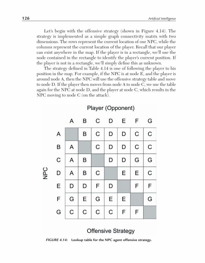
126 Artificial Intelligence
Let’s begin with the offensive strategy (shown in Figure 4.14). The strategy is implemented as a simple graph connectivity matrix with two dimensions. The rows represent the current location of our NPC, while the columns represent the current location of the player. Recall that our player can exist anywhere in the map. If the player is in a rectangle, we’ll use the node contained in the rectangle to identify the player’s current position. If the player is not in a rectangle, we’ll simply define this as unknown.
The strategy defined in Table 4.14 is one of following the player to his position in the map. For example, if the NPC is at node E, and the player is around node A, then the NPC will use the offensive strategy table and move to node D. If the player then moves from node A to node C, we use the table again for the NPC at node D, and the player at node C, which results in the NPC moving to node C (on the attack).
FIGURE 4.14: Lookup table for the NPC agent offensive strategy.

AI and Games 127
TIP The lookup table provides for reactive behaviors, as our NPC simply reacts to the movement of the player. Note that it’s also stateless, no state is kept between lookups, and the NPC simply uses its position and the player’s position to determine the next move.
The defensive strategy is shown in Table 4.15. This strategy is one of taking some time to heal by avoiding the player. Take, for example, the NPC at node D and the player again around node A. The lookup table returns a move from node D to node E, essentially putting distance between us and the player. If the player then moved to node D, the lookup table would return node F, moving away from an eventual move by the player to node E. Note that in some cases, the best move is to not move at all. If the NPC was at node G and the player at node B, the return value from the table is ‘-’ indicating to simply stay put.
FIGURE 4.15: Lookup table for the NPC agent defensive strategy.

128 Artificial Intelligence
While simple, this method gives us an efficient way to build offensive and defensive strategies for an NPC. No search is involved, simply table lookup. To add some level of unpredictability in the offensive strategy, the move could be selected randomly with some probability, rather than simply taking the lookup value.
NOTE Consider also the offensive strategy in Figure 4.14 as a path-finder to a given node. If we need to get from node G to node B, the lookup table takes us from node G to node C and then finally to node B. The lookup table in this way gives us a simple and efficient algorithm to get from point A to point B. This works well in static environments, but tends to fall apart if the environment changes over time.
In large environments, it can also be possible to segregate a map into multiple connected maps, each having funnel points for which an NPC may travel. Figure 4.16 shows a map of three zones. Rather than including a single lookup table for all points, three separate lookup tables would exist. If our NPC agent was in the left room, it could use the lookup table to determine which path to take to a given node. If the destination were outside of the room, it would by default move to node A, and from there, the external lookup table would take over for routing the NPC to its destination. If the
FIGURE 4.16: Segregating a map into separate zones to simplify path-finding.

AI and Games 129
destination were to the room on the right-hand side, the NPC would be directed to node B, and upon reaching node B, use its lookup table to get the rest of the way.
It’s also very common for these algorithms to time-slice their processing. This permits the work to be done over a number of iterations, without tying up the CPU on a single operation.
NPC BehaviorIn the last section, we gave our NPC the ability to traverse a map using strategies based on the NPC’s health (using intentional offensive and defensive strategies). Let’s now explore some options for giving our NPC the ability to behave intelligently in its environment.
The behavior of an NPC can’t be considered in isolation, because behavior is ultimately grounded in the environment. The NPC must be able to perceive its environment (see, hear, etc.). With the information perceived from the environment (as well as internal state information such as motivation), the NPC can reason about what should be done. The result of reasoning is potentially an intentional act, which is performed as an action (see Figure 4.17). This action (and subsequent actions) is what we externally view as the agent’s behavior.
FIGURE 4.17: The closed Loop of reasoning.
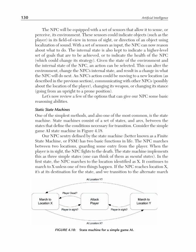
130 Artificial Intelligence
The NPC will be equipped with a set of sensors that allow it to sense, or perceive, its environment. These sensors could indicate objects (such as the player) in its field-of-view in terms of sight, or direction of an object using localization of sound. With a set of sensors as input, the NPC can now reason about what to do. The internal state is also kept to indicate a higher-level set of goals that are to be achieved, or to indicate the health of the NPC (which could change its strategy). Given the state of the environment and the internal state of the NPC, an action can be selected. This can alter the environment, change the NPC’s internal state, and result in a change in what the NPC will do next. An NPC’s action could be moving to a new location (as described in the previous section), communicating with other NPCs (possibly about the location of the player), changing its weapon, or changing its stance (going from an upright to a prone position).
Let’s now review a few of the options that can give our NPC some basic reasoning abilities.
Static State MachinesOne of the simplest methods, and also one of the most common, is the state machine. State machines consist of a set of states, and arcs, between the states that define the conditions necessary for transition. Consider the simple game AI state machine in Figure 4.18.
Our NPC sentry defined by the state machine (better known as a Finite State Machine, or FSM) has two basic functions in life. The NPC marches between two locations, guarding some entry from the player. When the player is in sight, the NPC fights to the death. The state machine implements this as three simple states (one can think of them as mental states). In the first state, the NPC marches to the location identified as X. It continues to march to X unless one of two things happen. If the NPC reaches location X, it’s at its destination for the state, and we transition to the alternate march
FIGURE 4.18: State machine for a simple game AI.

AI and Games 131
state. If the NPC sees the player, it attacks. If neither of these events occurs, the NPC continues marching.
When the NPC sees the player, by entering its field-of-view, the FSM transitions to the attack state. In this state, the NPC fights to the death. If the NPC dies, then the state machine is no longer active (the NPC lies lifeless in the environment). If the NPC defeats the player, it begins marching again toward location X.
There’s not much to the FSM, but they are simple and easy to debug. They are also very predictable, but it’s possible to add transition probabilities to give the NPC a small element of randomness.
Layered Behavior ArchitecturesOur previous FSM defined a very simple agent that had two things on its mind, marching and attacking. What was most important to the NPC was attacking, but while no player was in its field-of-view, it was quite happy to march back and forth. But what happens if our NPC has more things to worry about. If the NPC’s health is low, it should head to the infirmary. If the NPC is low on ammo, it should head to the armory to reload. If more than one player appears to attack, should it fight, or rush to the guard house to pull the alarm? These aren’t entirely complex, but the NPC now needs to engage in some thought to determine the most appropriate action for the given scenario.
One way to handle this conflict in action selection is Rodney Brooks’ subsumption architecture. This architecture confines responsibilities to isolated layers, but allows the layers to subsume one another if the need arises. Let’s look at our simple NPC again to see how we might map the new refined behaviors into subsumption (see Figure 4.19).
FIGURE 4.19: Behavior layers for the simple NPC.

132 Artificial Intelligence
Figure 4.19 illustrates one example of our NPC’s requirements to a layered architecture. These levels should be viewed in relative importance. At level one, our NPC performs his guard duty, dutifully marching along his route. If the player comes into view, the NPC switches to the attack layer to rid the environment of the pesky player. From Brookes’ architecture, the Attack layer subsumed (took priority over) the March layer. If no players are in the field-of-view, and the NPC needs to be healed or replenish his ammunition, the sustain layer takes over to perform those actions. Finally, the NPC will turn to the survive layer if more than one player is seen in the field-of-view. As the constraints are met within the layers, the NPC will default to the lowest layer. Therefore, once the player is disposed of, and the ammo and health are returned, the NPC will return to the march in level one.
Within each of these layers, individual FSMs can be used to implement the relevant behavior. In this way, entirely new state machines are consulted based on the current behavior layer for the NPC.
NOTE An interesting analogy to NPCs in video games is the field of Intelligent Agents. We’ll explore the field of Intelligent Software Agents in Chapter 11.
Other Action-Selection MechanismsWe’ll discuss other relevant algorithms that could be used to select an action for an NPC in the following chapters. Neural networks are an interesting example of behavior selection (classification), as are planning algorithms and numerous other machine-learning algorithms (reinforcement learning, to name one). The machine-learning algorithms are of particular interest as they can instill the ability for the NPC to learn and behave in new ways given previous encounters with the player.
NOTE In a typical game, a game engine provides the base platform for graphics and fundamental game-play. The NPC behaviors are commonly implemented using high-level scripts, with a script interpreter implemented within the game engine. This provides a great amount of flexibility, where the game engine is implemented in a high-level language such as C or C++ for efficiency, and the NPC behaviors are implemented in a scripting language for flexibility.
Team AIIn many games, there’s not just a single NPC soldier that we’re fighting against, but an entire army that must work together in harmony with a single

AI and Games 133
or handful of goals in mind. The control can exist at a number of levels within a hierarchy (see Figure 4.20), from the squad leader directing troops to flank an enemy in the field using real-time battlefield information, to the general managing his entire army to implement the higher-level military strategies.
Managing an overall army can entail a large number of problems, from scheduling and production, to resource allocation, to the overall strategy and tactics of the force in the field.
The problem here can be simplified greatly by minimizing the number of levels or organization. First, the individual soldiers simply follow orders, and unless they are routed, can fight to the death. These individual units can be programmed using finite state machines, or other simple mechanisms for behavior.
TIP Following orders is a requirement, but there’s also something to be said for autonomy at the soldier level, taking advantage of a local situation to improve the chances of a global win.
The problem to solve then is the higher-level control of the entire force. This can be subdivided as well, especially when forces are split for independent goals. At the highest level is the Strategic AI. This layer of the AI has the
FIGURE 4.20: Organizational structure of a simplified army.

134 Artificial Intelligence
global view of the battlefield, troop strengths, available resources, etc. Next is the Tactical AI whose job is to implement the strategy provided from above. At the lowest rung is the individual soldier, on whose collective shoulders that overall strategy relies.
NOTE For this discussion, we’ll focus on Team AI that opposes a human player, but much of this can also be applied to Team AI that cooperatively supports the player, though this can be considerably more difficult. For example, working cooperatively with the player requires that the NPC help, but also stay out of the player’s way.
Goals and PlansAn interesting mechanism for high-level control over a hierarchy of military units is in defining a goal, and then creating a plan to reach that goal. Also necessary is the need to reformulate a plan, when it eventually fails.
Let’s first discuss the planning vernacular and then explore how it can be applied to team AI. First, there’s the goal. A goal can be an end-goal (for the end of the game) or an intermediate goal that moves us closer to an end-game situation. Formally, a goal is a condition that is desired to be satisfied. Example goals include taking an enemy position, destroying a bridge, flanking an enemy, etc. To reach a goal, we must perform a series of
FIGURE 4.21: The plan and its elements.
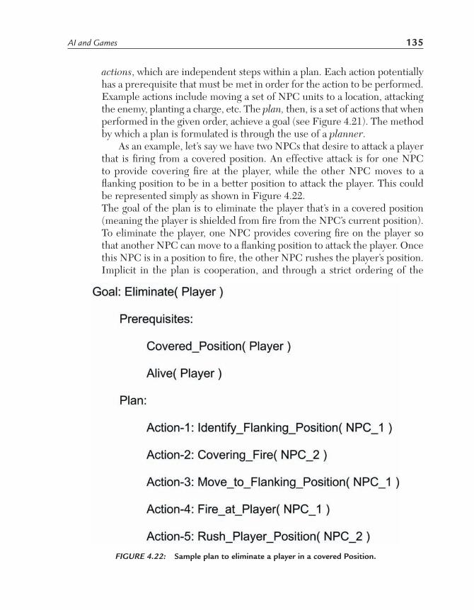
AI and Games 135
actions, which are independent steps within a plan. Each action potentially has a prerequisite that must be met in order for the action to be performed. Example actions include moving a set of NPC units to a location, attacking the enemy, planting a charge, etc. The plan, then, is a set of actions that when performed in the given order, achieve a goal (see Figure 4.21). The method by which a plan is formulated is through the use of a planner.
As an example, let’s say we have two NPCs that desire to attack a player that is firing from a covered position. An effective attack is for one NPC to provide covering fire at the player, while the other NPC moves to a flanking position to be in a better position to attack the player. This could be represented simply as shown in Figure 4.22.The goal of the plan is to eliminate the player that’s in a covered position (meaning the player is shielded from fire from the NPC’s current position). To eliminate the player, one NPC provides covering fire on the player so that another NPC can move to a flanking position to attack the player. Once this NPC is in a position to fire, the other NPC rushes the player’s position. Implicit in the plan is cooperation, and through a strict ordering of the
FIGURE 4.22: Sample plan to eliminate a player in a covered Position.

136 Artificial Intelligence
actions, coordination. Later, we’ll see how planning is achieved (and like much of AI, it’s fundamentally a search problem).
NOTE Implicit in planning are preconditions (or prerequisites) that must be met in order for the plan to be valid. Consider the plan in Figure 4.22 if only one NPC is present. What happens if NPC_1 is eliminated while on the move to its flanking position? Preconditions must be met for a plan to be valid, and if at any time actions in a plan cannot be performed, the plan cannot continue. Therefore, in dynamic environments, planning and replanning go hand-in-hand.
Real-Time Strategy AIA final interesting use of AI is in the development of real-time strategy games. Real-Time Strategy AI differs from Team AI in that we will deal not only with the militaristic aspects of the game, but also the economic aspects. For example, in a real-time strategy game, elements of the civilization must engage in resource gathering as part of a higher-level goal of building an army to defeat an opponent.
For example, in the beginning of a real-time strategy game, the focus is societal and military buildup. This involves creating new citizens to build the economy. Once the economy reaches a certain level, a military buildup can occur to attack and defeat an enemy.
The conditions described could be embedded within the game engine itself, but for flexibility, could be implemented separately permitting ease of modification without having to rebuild the game engine. One possibility that’s been used in the past is Rule-Based Systems (or RBS).
Rule-Based ProgrammingRule-based systems are an effective way to encode expert knowledge about game play into a strategy game. Rule-based systems are so interesting that a standards committee has been formed to study their use in games. [IGDA 2005]
NOTE We’ll explore rule-based programming as part of the review of knowledge representation in Chapter 6.
A rule-based system is made up of two memories, one that holds facts, and another that holds a set of rules that exist to determine the behavior. A rule-matching algorithm is applied to the facts, and those rules that match facts are saved into the conflict-set. This set of rules is then reviewed and

AI and Games 137
one rule picked to fire in a process called conflict resolution. The rule is then applied and the working memory is updated.
NOTE Selecting a rule to fire from a list of rules that have matched can use a number of algorithms. One could select at random, the last rule to match, or the rule that’s most specific (had the largest number of conditions).
FIGURE 4.23: Typical flow of a rule-based system.

138 Artificial Intelligence
Now that we’ve explored the process, let’s look at the anatomy of facts and rules. A fact is an atomic element of knowledge that can be used in conjunction with other facts to reason using rules. Facts can take on a variety of forms; one of the most common is the S-expression (or Symbolic Expression), which simply is a way of structuring the data. Consider the following four facts in our simple knowledge base:
(opponent-1 size large) (opponent-2 size small) (army size large)
Regarding our game world, these facts tell us that the first opponent is large in size, the second opponent is small, and our army is also considered large. Before looking at some rules given our small knowledge base, let’s review the structure of a rule.
Rules are made up of two things, antecedents and consequents. If you think about a rule as an if/then construct, then the ‘if’ is the antecedent, and the ‘then’ is the consequent. Consider the following simple comparison:
if ((opponent.size <= SMALL_SIZE) && (army.size >= LARGE_SIZE)) { attack_opponent(); }
This conditional simply says that if the opponent’s military size is small, and ours is large, we’ll attack them. A simple rule that encodes this behavior could be implemented as follows:
(rule “Attack Opponent Based Upon Size” (?opponent size small) (army size large) ==> (army attack ?opponent) )
Note that the ‘?opponent’ element will match any opponent in the working memory, and when it matches one, we’ll use this same opponent when attacking. Once this rule fires, our working memory will exist as: (opponent-1 size large) (opponent-2 size small) (army size large) (army attack opponent-1)

AI and Games 139
This new fact would drive behavior within the game engine to formulate a plan to attack the enemy. The RBS could also remove facts as driven by consequents to reflect the dynamic environment of the game.
TIP To deal with sizes, the RBS can ‘fuzzify’ values from ranges to distinct sets. For example, the size used in the previous examples could identify the range [0..4999] as small, [5000..9999] as medium, and [10000..50000] as large. This reduces the complexity of the inputs and simplifies the rules base.
An RBS is a useful method for encoding knowledge into a game that can be used to drive behaviors, especially high-level behaviors in matters of strategy. It’s also advantageous because it allows the strategy element to be decoupled from the game engine and permits later tweaking by game developers.
CHAPTER SUMMARY
This chapter provided a broad spectrum of techniques used in game AI, from classical games, to modern video games. In classical games such as Chess and Checkers, and even information imperfect games such as Poker, the minimax game-tree search algorithm with alpha-beta pruning can be found. In these games, the goal of developers is to build an opponent that can defeat world-class players. In contrast, the goal in video games is to build opponents that are challenging to play, but not perfect. Even with this limitation in mind, various AI technologies can be found in modern games, from neural networks, to rule-based systems and decision trees, to embed game opponents that are both challenging and adaptive to the human’s level of play.
REFERENCES
[AI Horizon] Available online at:http://www.aihorizon.com/essays/chessai/boardrep.htm [AI Chess] Available online at:http://www.cs.cornell.edu/boom/2004sp/ProjectArch/Chess/algorithms.
html [Archer 1999] Archer, A.F. “A Modern Treatment of the 15 Puzzle,”
American Math. 106:, 793-799, 1999.

140 Artificial Intelligence
[Anderson 2005] Anderson, Gunnar. “Writing an Othello program,” Available online at:
http://www.radagast.se/othello.[Chellapilla, Fogel 2000] Chellapilla, Kumar and Fogel, David B. “Anaconda
Defeats Hoyle 6-0: A Case Study Competing an Evolved Checkers Program against Commercially Available Software (2000).” Proceedings of the 2000 Congress on Evolutionary Computation CEC00.
[IGDA 2005] “Working Group on Rule-based Systems,” AI Interface Standards Committee, The 2005 AIISC Report, 2005. Available online at:
http://www.igda.org/ai/report-2005/rbs.html[Johnson 1997] Johnson, George. “To Test a Powerful Computer, Play an
Ancient Game.” Introduction to Computation and Cognition. Available online at:
http://www.rci.rutgers.edu/%7Ecfs/472_html/Intro/NYT_Intro/ChessMatch/ToTest.html
[Loki 2003] Jonathan Schaeffer, Darse Billings, Lourdes Pena, Duane Szafron. “Learning to Play Strong Poker.” 2003.
[Lu 1993] Lu, Chien-Ping Paul. “Parallel Search of Narrow Game Trees.” Master’s thesis, University of Alberta, Department of Computing Science, Edmonton, Canada, 1993.
[McCarthy 1990] Available online at:http://www-db.stanford.edu/pub/voy/museum/samuel.html[Samuel 1959] Samuel, A. L. “Some Studies in Machine Learning using
the Game of Checkers,” IBM Journal of Research and Development, 1959.
[Shannon 1950] J. Schaeffer “1989 World Computer Chess Championship,” Computers, Chess and Cognition, Springer-Verlag, New York, 1990.
[Sutton/Barto 1998] Sutton, Richard S., and Barto, Andrew G. “Reinforcement Learning: An Introduction.” MIT Press, 1998.
RESOURCES
Bruce Moreland’s Chess Programming Topics. Available online at:http://www.seanet.com/~brucemo/topics/topics.htm[Chinook] Available online at:http://www.cs.ualberta.ca/%7Echinook/The Intelligent Go Foundation. Available online at:http://intelligentgo.org/en/computer-go/overview.html

AI and Games 141
Bouzy, Bruno and Cazenave, Tristan. “Computer Go: an AI Oriented Survey.” Universite Paris.
Brooks, Rodney. “A Robust Layered Control System for A Mobile Robot,” IEEE Journal of Robotics and Automation RA-2, April 1986.
Tesauro, Gerald. “Temporal Difference Learning and TD-Gammon.” Available online at:
http://www.research.ibm.com/massive/tdl.htmlTD-learning, Neural Networks, and Backgammon. Available online at:http://www.cs.cornell.edu/boom/2001sp/Tsinteris/gammon.htm[Sheppard 2002] Sheppard, Brian. “World-championship-caliber
Scrabble,” Artificial Intelligence 134: (2002), 241-275.
EXERCISES
1. What is meant by adversarial search, and how does it differ from traditional tree search?
2. What is ply in game-tree search?3. Given the game tree shown in Figure 4.24, what is the value at the root
node?4. Minimax can search to the leaves of the tree, or to a predefined depth.
What are the consequences of ending a search at a predefined depth?
FIGURE 4.24: Sample game tree for minimax search.

142 Artificial Intelligence
5. Given the game tree shown in Figure 4.25, what is the value at the root node and which nodes are pruned from the search?
6. What was the first successful game-playing program that used self-play to learn an effective strategy?
7. Explain what is meant by perfect-information and imperfect-information games. Give a few examples of each, and define which type they are.
8. Define some of the similarities and differences for building a game-playing AI for Checkers and Chess.
9. What are some of the major differences between building AI for classical games and video games?
FIGURE 4.25: Sample game tree for minimax search with alpha-beta pruning.