Embed Size (px)
Citation preview
BASIC PILE GROUP BEHAVIOR.(U)DEC 80 i HARTMAN
UNCLASSIFIED WES-TRAK-80-5 Ft.*2flflflflflflflflflflflIIIEIIhI-IIImlEEEilllilllIIIIIIIIIIIIIIIlIIIIIIIIIIIIIIElEllEEEElhihE

-wiiii W.
136
11111 1.5~11A111.6IC11 IIIIIO iST CHAR.
MICROCOPY RESOLUTION TEST CHART

BASIC,:PILE GROUP BEHAVIORby
The CMS Task &a on. M QTICi
A4kwpwt end., the C.putorde ~sauuP _____ E~gluwmh(CASE) Pt*cd
PI()"'fog* , -fi#
~ b. gu hi o forkger needed. retum. It ito
414 aisds in ti's report are -not to b. construed as an officialDNpwvot'of the Army position unless so disignatbd
by other authorized docuients.
The mutiWts ofA ahi rmor aeno t be ugsgd for.dwrttefrt, p*ebte"On, of promotional P""rp
Sif O*vdMt e4eW'oo apfdV~lo s*o
'r jr~1 . ..
UnclassifiedSECURITY CLASSIFICATION OF TIlS PAGE (Wan, Daea RAIM6 ADV Mr 8
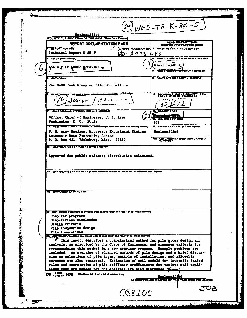
REPORT DOCUMENTATION PAGE 8MZCNLM o1. REPORT NUMISMR .. .GOVT ACCESSION NO. RECIPIENT'S CATALOG NU#A§ER
Technical Report K-80- 5 o ' 94L TITLE (And Sabdife) a VOT&PRO OEE
4BJASIC Final reRDW
AUTHO~fQ S. CONTRACT Olt GRANT NUM1111e.)
The CASE Task Group on Pile Foundations
NIZA R.."_R w aorta IS. P:OGRAM ELEMENT, PROJECT. TAMK(~~~II~ AA 6 W0RK UNIT NUMINERS
11. CONTROLLING OFFICR NME AND ADDRESS aMR-~*-
Office, Chief of Engineers, U. S. Army 010 I SRO AEWashington, D. C. 2031416
14. MONITORING AGENCY NAMES& AORESS~a AM..., kr Cautiveflhtd OW..) 1S. SECURITY CLASS. (of ma re t
U. S. Army Engineer Waterways Experiment Station UnclassifiedAutomatic Data Processing Center______________P. 0. Box 631, Vicksburg, Miss. 39180 ISAL DECASICATION/OWNGRADING
IC. DISTRIBUTION STATEMENT (of Nia Repea)
Approved for public release; distribution unlimited.
17. DISTRIMUTION STATEMENT (of jIh. ab"jrwA eteed i Blook 20. It EfffeaU hem Repeat)
IS. SUPPLEMENTARY NOTES
to. KEY WORDS (Coa*hu - mm.. Oe~ It neeo40MY and IdenII& by wleek embew)
Computer programsComputerized simulationDesign criteriaPile foundation designPile foundations
0, ACj -omemS N.mph ~ ymbeak ubm)
n This report describes a computerized method for pile group design andanalysis, as practiced by the Corps of Engineers, and proposes criteria forsystematizing this method In a new computer program. Example problems areincluded. An overview of advanced methods of pile design and a brief discus-sion on selections of pile types, methods of installation, and allowablestresses are also presented. Estimation of soil moduli for laterally loadedpiles and computation of pile stiffness coefficients for various soil condi-
tin that menermvs
FO M sMM rfnw 117 min nlsii
PREFACE
This report describes a computerized method for analysis and
design of pile groups that is currently being used by several Corps of
Engineers offices. Criteria for a new, comprehensive computer program
for pile analysis and design are also discussed. The work was sponsored
under funds provided to the U. S. Army Engineer Waterways Experiment
Station (WES) by the Office, Chief of Engineers (OCE), under the
Computer-Aided Structural Engineering (CASE) Project.
The report was compiled by the CASE Task Group on Pile Foundations.
Members and others who directly contributed to the report were:
James G. Bigham, New Orleans District (Chairman)Roger Brown, South Atlantic DivisionRichard M. Chun, Pacific Ocean DivisionDonald R. Dressler, OCERixby J. Hardy, OCE_loaepk Hartman, St. Louis DistrictRoger Hoell, St. Louis DistrictH. Wayne Jones, WESReed L. Mosher, WESPhilip Napolitano, New Orleans DistrictN. Radhakrishnan. WESCharles Ruckstuhl, New Orleans DistrictArthur T. Shak, Pacific Ocean DivisionRalph Strom, Portland District
Compilation of this report was done by Mr. Hartman. Messrs. Dres-
sler, Structures Branch, and Hardy, Geotechnical Branch, Civil Works
Directorate, were OCE points of contact. Dr. Radhakrishnan, Special
Technical Assistant, Automatic Data Processing (ADP) Center, WES, is
CASE Project Manager. He monitored the work under the supervision of
Mr. Donald L. Neumann, Chief of the ADP Center.
Director of WES during the period of development and the publica-
tion of this report was COL N. P. Conover, CE. Technical Director was
Mr. F. R. Brown. (D -!I0 0
to 'U
I
CONTENTS
Page
PREFACE ....... ...... .............................. 1
CONVERSION FACTORS, INCH-POUND TO METRIC (SI)UNITS OF MEASUREMENT ....... .... ....................... 3
I. SCOPE ....... ...... ............................ 4
II. PILE DESIGN CONSIDERATIONS ...... .................. 4
A. Economic _ 4........................4B. Affect on Adjacent Structures. .............. 4C. Difficulty in Installation ....... ............... 4D. Environment ....... .. ....................... 4E. Displacements ......... ...................... 5F. Foundation Materials ....... .. .................. 5G. Failure Nodes ....... .... ..................... 5H. Other Considerations ....... .. .................. 6
III. BASIC PILE GROUP ANALYSIS ....... .. ................. 6
A. Basic Analysis Method ........ .................. 6B. Pile-Structure Interaction ........ .............. 7C. Pile-Soil Interaction ....... .. .................. 8D. Analysis Details ....... .................... ... 10E. Limitations ....... .. ...................... ... 14F. Sample Analyses ........ .................... ... 14
IV. COMPUTER PROGRAM CRITERIA ...... ................. ... 15
A. General Requirements ....... .................. ... 15B. Program Operation ....... .................... ... 16C. Pile Layout Input ....... .. .................... 17D. Pile Property Input ...... ................... ... 17E. Pile Allowable Loads ..... .................. 18F. Applied Loads ....... ...................... .. 18G. Output ....... .... ......................... 19H. Pre-Processors and Post-Processors ... ........... ... 19
V. ADVANCED ETHODS OF PILE DESIGN ....... ............... 1'9
A. PILEOPT Program ....... ..................... ... 19B. Flexible Base Analysis ...... ................. ... 20C. Non-Linear Analysis ...... ................... ... 20
REFERENCES ........... ............................ . 21
APPENDIX A: PILE TYPES AND ALLOWABLE STRESSES ..... .......... Al
APPENDIX B: PILE INSTALLATION METHODS ....... .............. B1
APPENDIX C: PILE STIFFNESS COEFFICIENTS ..... .............. Cl
APPENDIX D: SOIL MODULUS FOR LATERALLY LOADED PILES ... ....... DI
APPENDIX E: EXAMPLE PROBSUS ........ ................... El
, 1.1e
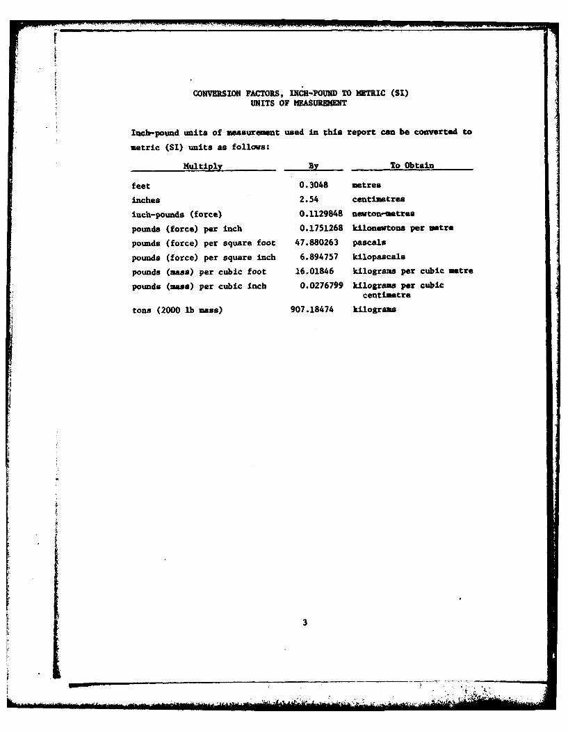
CONVERSION FACTORS, INCI-POUND TO )MTRIC (SI)UNITS OF MEASUREMENT
Inch-pound units of measurement used in this report can be converted to
metric (SI) units as follows:
Multiply By To Obtain
feet 0.3048 metres
inches 2.54 centimetres
inch-pounds (force) 0.1129848 newton-metres
pounds (force) per inch 0.1751268 kilonewtons per metre
pounds (force) per square foot 47.880263 pascals
pounds (force) per square inch 6.894757 kilopascals
pounds (mass) per cubic foot 16.01846 kilograms per cubic metre
pounds (mass) per cubic inch 0.0276799 kilograms per cubiccentimetre
tons (2000 lb mass) 907.18474 kilograms
3
I. SCOPE.
The purpose of this paper is to present one method for pile group
design and analysis as practiced by the Corps of Engineers, and to propose
criteria for systematizing this method in a computer program. This paper
describes a computerized method of pile group analysis (including sample
problems) and lists criteria for a new, more comprehensive program; it
includes an overview of advanced methods of pile design, and briefly
discusses selection of pile types, methods of installation, and allowable
stresses
II. PILE DESIGN CONSIDERATIONS.
A. Economic. Pile foundations are a major cost in a structure. Pile
foundations that provide the lowest first cost are of paramount importance.
A cost comparison must be made of the relative cost of different type piles
and cost of installation. Scheduling and availability may affect pile
costs. Details affecting selection of pile type are presented in Appendix A.
B. Affect on Adjacent Structures. Proximity of adjacent structures
may dictate the type of pile or installation used. Adverse effects of soil
displacement or vibration caused by driving piles may compel the use of
drilled caissons, nondisplacement piles, or jetting or predrilling of piles.
C. Difficulty in Installation. Hard strata, boulders, buried debris,
and other obstructions may necessitate the use of piles durable enough to
sustain driving stresses. Jetting, predrilling, or spudding may be
required. Oescriptions of installation methods are presented in Appendix B.
D. Environment. Corrosion in sea water will require consideration for
protective coating, concrete jacketing, or cathodic protection if steel
piling is used. The presence of marine-borers may negate the use of wood
piling and the subsequent use of steel or concrete piling.
4
E. Displacements. Limitations on lateral or rotational movement will
affect the type of pile used and the configuration of the pile group.
Stiffer piles and the degree of fixity to the pile caps are considerations to
limit displacements.
F. Foundation Materials. The capacity of the piling may be limited by
failure of the foundation materials, evidenced by excessive settlement of
piles under applied load. The capacity of the foundation materials is
usually evaluated by static resistance formulas during design and verified by
load tests prior to construction. Dynamic driving formulas are generally not
a reliable basis for estimating pile capacities unless correlated with load
tests and previous experience at similar, nearby sites. More reliable
predictions of dynamic behavior during driving are based on complex
computerized models of ha- er-pile-soil- interaction using the ID wave
equation.
G. Failure Modes.
1. Bearing capacity failure of the pile-soil system.
2. Excessive settlement due to compression and consolidation of
the underlying soil.
3. Structural failure of the pile under service loads.
4. Bearing capacity failure caused by improper installation
methods.
5. Structural failure resulting from detrimental pile
installation. This may be due to unforseen subsoil conditions or to freeze,
compaction, liquification, or heave of the soil. It could be caused by
driving sequence, size of hammer, vibration, over or under driving, improper
preexcavation methods, substitution of materials, improper workmanship, or
5
limitations of the Contractor% equipment or expertise. These conditions are
described in detail in Chapter 2 of Reference 1.
H. Other Considerations. For more detailed discussion of the above
considerations, and for others not mentioned above, see Reference 2.
III. BASIC PILE GROUP ANALYSIS.
This section presents the fundamentals of a basic method of pile group
analysis which is currently available in various computer programs including
LMVDPILE which is in WESLIB. Several hand analysis methods are shown with
the sample problems in Appendix E. This computer method is capable of
handling three-dimensional loading and pile geometry. It is valid for static
analysis of a linear, elastic system. Interaction between pile and structure
is limited to the extremes of a fully fixed or fully pinned connection.
Interaction between the pile and soil is represented by a linear, elastic
pile stiffness (applied load per unit deflection) at the top of the pile.
The base of the structure is assumed to act as a rigid body pile cap
connecting all piles; the cap flexibility is not considered.
A. Basic Analysis Method. The basic pile group analysis method
represents each pile by its calculated stiffness coefficient, in the manner
proposed by iaul (3). The stiffness coefficients of all piles are summed to
determine a stiffness matrix for the total pile group. Displacements of the
rigid pile cap are determined by multiplying the sets of applied loads by the
inverse of the group stiffness matrix. Displacements of the rigid pile cap
define deflections of individual pile heads which are then multiplied by the
pile stiffness coefficients to determine the forces acting on each pile
head. The key step in the method is in determining individual pile stiffness
coefficients, at the pile head, based on known or assumed properties of pile
6
and soil. Since this is a three-dimensional analysis method, each pile head
has six degrees of freedom (DOF), three translations and three rotations. A
stiffness coefficient must be determined for each DOF and for all coupling
effects (e.g. lateral deflection due to applied moment). The pile location
and batter angle are also accounted for when individual pile stiffness
coefficients are combined to form the total stiffness matrix for the pile
group.
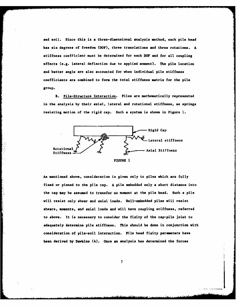
B. Pile-Structure Interaction. Piles are mathematically represented
in the analysis by their axial, lateral and rotational stiffness, as springs
resisting motion of the rigid cap. Such a system is shown in Figure 1.
Rigid Cap
Lateral stiffness
RotationalAilStfnsStiffnessij xa tfns
FIGURE 1
As mentioned above, consideration is given only to piles which are fully
fixed or pinned to the pile cap. A pile embedded only a short distance into
the cap may be assumed to transfer no moment at the pile head. Such a pile
will resist only shear and axial loads. Well-embedded piles will resist
shears, moments, and axial loads and will have coupling stiffness, referred
to above. It is necessary to consider the fixity of the cap-pile joint to
adequately determine pile stiffness. This should be done in conjunction with
consideration of pile-soil interaction. Pile head fixity parameters have
been derived by Dawkins (4). Once an analysis has determined the forces
7
acting on each pile, these forces may then be applied to the pile cap to
determine its internal shears and moments. However, analysis of the pile cap
is outside the scope of this section.
C. Pile-Soil Interaction. Interaction between the pile and soil is
the most important consideration in determining pile stiffness. Therefore,
it is necessary to have reliable information about soil properties. Soil
properties can affect the axial, lateral, or torsional stiffness of the
pile. The type of loading expected (static or cyclic) and the pile spacing
should also be considered since cyclic loading or close spacing may both
reduce individual pile stiffness.
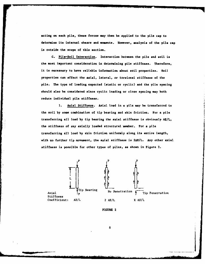
1. Axial Stiffness. Axial load in a pile may be transferred to
the soil by some combination of tip bearing and skin friction. For a pile
transferring all load by tip bearing the axial stiffness is obviously AE/L,
the stiffness of any axially loaded structural member. For a pile
transferring all load by skin friction uniformly along its entire length,
with no further tip movement, the axial stiffness is 2AE/L. Any other axial
stiffness is possible for other types of piles, as shown in Figure 2.
p P p
LL H
Tip Bearing No Penetration
Axial PTip PenetrationStiffness
Coefficient: AE/L 2 AE/L K AE/L
FIGURE 2
8
A further complication of pile axial stiffness involves consideration of
tension piles. Generally, a pile in tension will be less stiff than the same
pile in compression. Since only a single elastic stiffness coefficient may
be specified for each pile, that stiffness must be based on whether the load
is expected to be tension or compression.
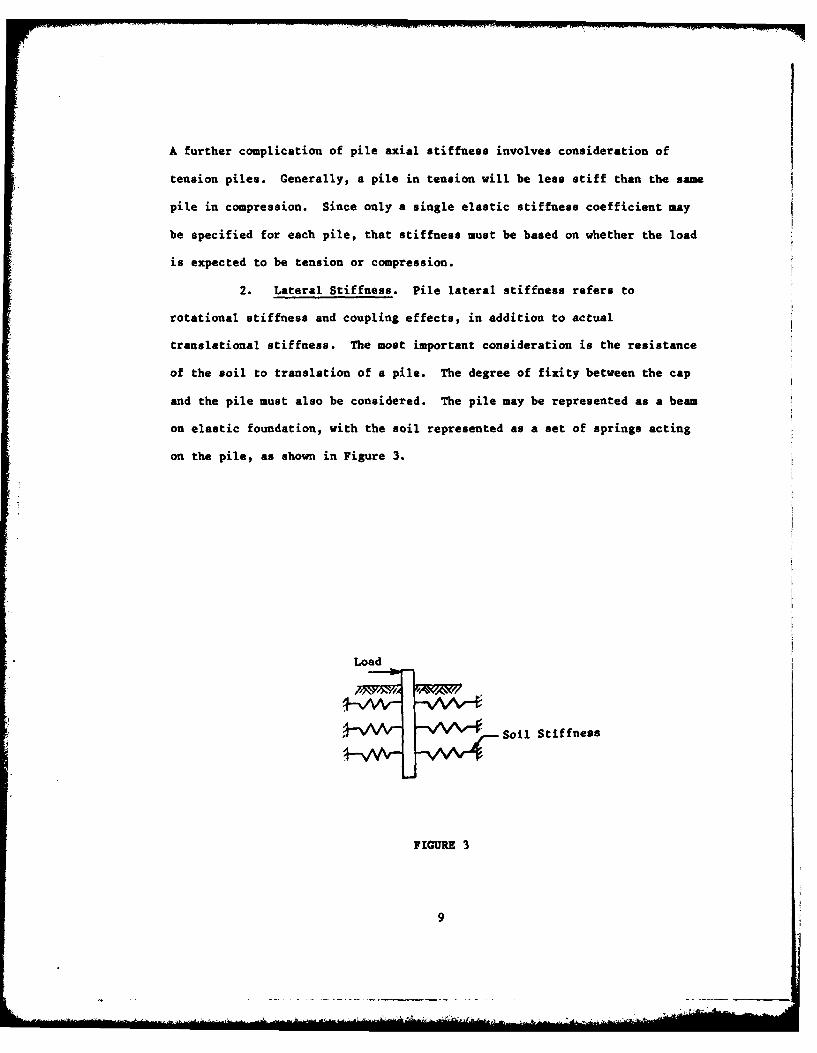
2. Lateral Stiffness. Pile lateral stiffness refers to
rotational stiffness and coupling effects, in addition to actual
translational stiffness. The most important consideration is the resistance
of the soil to translation of a pile. The degree of fixity between the cap
and the pile must also be considered. The pile may be represented as a beam
on elastic foundation, with the soil represented as a set of springs acting
on the pile, as shown in Figure 3.
Load
Soil Stiffness
FIGURE 3

Though soil properties are often highly non-linear, an approximate linear
lateral stiffness coefficient must be determined. Several analytical methods
may be used to determine this stiffness. One method is to use any beam
analysis computer program capable of representing the beam-spring system
shown in Figure 3. The stiffness equals the force required to cause a unit
displacement at the pile head. This method may be used to determine lateral,
rotational and coupling stiffness coefficients. A method for determining
appropriate values for the stiffness of the soil springs is included as
Appendix D. Methods for determining pile stiffness coefficients are
presented in detail in Appendix C.
3. Torsional Stiffness. For groups of piles, torsion on
individual piles is usually unimportant and may be neglected by using zero
torsional stiffness. Where torsion of individual piles is important,
torsional stiffness may be determined in a manner similar to that described
above for axial stiffness (5).
D. Analysis Details. As mentioned above, this analysis method has
been systematized for use in computer programs. Several of these programs
were identified during the Corps-Wide Conference on Computer Aided Design in
Structural Engineering (6). Following are some of the detailed formulations
used in these programs.
1. Coordinate System. The basic coordinate system is a right
hand system, as shown in Figure 4. The three axes are labeled 1, 2, and 3,
with the 3 axis being positive downward. This global coordinate system is
used for specification of pile locations and orientations, applied forces and
10
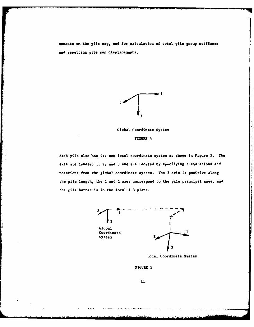
moments on the pile cap, and for calculation of total pile group stiffness
and resulting pile cap displacements.
3
Global Coordinate System
FIGURE 4
Each pile also has its own local coordinate system as shown in Figure 5. The
axes are labeled 1, 2, and 3 and are located by specifying translations and
rotations from the global coordinate system. The 3 axis is positive along
the pile length, the 1 and 2 axes correspond to the pile principal axes, and
the pile batter is in the local 1-3 plane.
Global
System 2
3
Local Coordinate System
FIGURE 5
11
The local coordinate system is used for calculation of the stiffness
coefficients, displacements, and forces of individual piles.
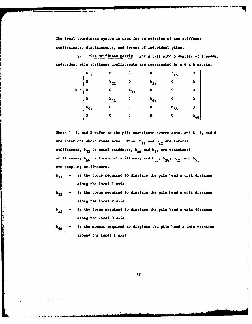
2. Pile Stiffness Matrix. For a pile with 6 degrees of freedom,
individual pile stiffness coefficients are represented by a 6 x 6 matrix:
bl1 0 0 0 b 15 0
0 b22 0 b24 0 0
b 0 0 b33 0 0 0
0 b42 0 b44 0 0
b5 1 0 0 0 b55 0
0 0 0 0 0 b66
Where 1, 2, and 3 refer to the pile coordinate system axes, and 4, 5, and 6
are rotations about those axes. Thus, b11 and b2 2 are lateral
stiffnesses, b33 is axial stiffness, b4 and b55 are rotational
stiffnesses, b66 is torsional stiffness, and b15 , b24 , b42 , and b5 1
are coupling stiffnesses.
b 11 - is the force required to displace the pile head a unit distance
along the local I axis
b22 - is the force required to displace the pile head a unit distance
along the local 2 axis
b - is the force required to displace the pile head a unit distance
along the local 3 axis
b - is the moment required to displace the pile head a unit rotation
around the local 1 axis
12
b55 - is the moment required to displace the pile head a unit rotation
around the local 2 axis
*b15 - is the force along the local 1 axis caused by a unit rotation of
the pile head around the local 2 axis
*b24 - is the force along the local 2 axis caused by a unit rotation of
the pile head around the local 1 axis
*b - is the moment around the local 2 axis caused by a unit displacement
of the pile head along the local 1 axis
*b - is the moment around the local 1 axis caused by a unit displacement42
of the pile head along the local 2 axis
j
*Since the stiffness matrix must be symmetric b15 - b5 1 and b24
b42 . The sign of b24 and b42 must be negative.
Generally, each stiffness coefficient is influenced by the effects of
pile-structure and pile-soil interaction. For example, bll may be defined
as:
b11 -C1 C 2
Where C 1 is a constant depending on the pinned or fixed condition
at the pile head and C2 is a constant based on pile-soil interaction.
Depending on the method used, these terms may be calculated separately and
then multiplied to determine the pile stiffness coefficient, or the entire
stiffness may be determined directly.
3. Analysis Method. The stiffness matrix of each pile is
transformed from the local coordinate system to the global coordinate
system. All pile stiffness matrices are then sumed to form a 6 x 6 matrix
13

representing the stiffness of the entire pile group. Applied loads are
defined as a set of three forces and three moments acting on the pile cap.
To determine displacements of the pile cap the following equation must be
solved:
[F] - (K] (u]
Where F is the applied load set, K is the pile group stiffness matrix, and U
is the set of pile cap displacements. Once these displacements have been
determined, the displacements at the head of each pile can be determined by a
geometric transformation based on the location and orientation of that pile.
The following equation must then be solved to determine forces acting on each
pile head:
(f] - (b] [u]
Where f is the set of pile loads, b is the pile stiffness coefficients, and u
is the set of pile head displacements. The above represents the basic
analysis of a pile group. Further details are contained in the user's
manuals for the various computer programs.
E. 'imitations. Most of the limitations of this method of pile group
analysis have been mentioned above, but will now be summarized. The method
is valid for static analysis of a linear, elastic system. Applied loads must
be equivalent static loads, non-linear soil properties must be represented by
linear pile behavior. The other major limitation is that the pile cap is
assumed to be rigid. Though this may be a valid assumption for a massive
structure, such as a dam pier, it may result in gross errors in long, thin
structures, such as a U-frame lock monolith.
F. Sample Analyses. Several sample problems are shown in Appendix E,
solved by the above method and by conventional hand methods.
14
IV. COMPUTER PROGRAM CRITERIA.
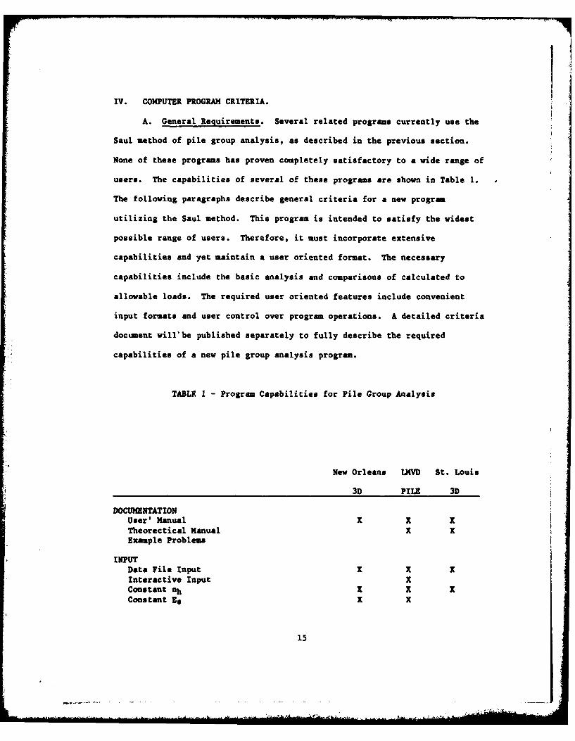
A. General Requirements. Several related programs currently use the
Saul method of pile group analysis, as described in the previous section.
None of these programs has proven completely satisfactory to a wide range of
users. The capabilities of several of these programs are shown in Table 1.
The following paragraphs describe general criteria for a new program
utilizing the Saul method. This program is intended to satisfy the widest
possible range of users. Therefore, it must incorporate extensive
capabilities and yet maintain a user oriented format. The necessary
capabilities include the basic analysis and comparisons of calculated to
allowable loads. The required user oriented features include convenient
input formats and user control over program operations. A detailed criteria
document will'be published separately to fully describe the required
capabilities of a new pile group analysis program.
TABLE I - Program Capabilities for Pile Group Analysis
New Orleans LMVD St. Louis
3D PILE 3D
DOCUMENTATIONUser' Manual X X XTheorectical Manual X XExample Problems
INPUTData File Input X X XInteractive Input XConstant nh X X XConstant Eg X X
15

TABLE 1 - Program Capabilities for Pile Group Analysis (continued)
New Orleans LMVD St. Louis3D PILE 3D
INPUT (continued)Layered EaDirect b-- Input X XFile Coordinate Generation X X
ANALYSISSaul 2DSaul 3D X X XVettersTension Pile InterationChecks Calculated vsAllowable Loads X X
OUTPUTInput Echo X X XPile Stiffness Coefficients X X XPile Group Stiffness Matrix X X XElastic Center X XStructure Deflections X X XPile Deflections X XPile Forces X X XPile Force Components X XSum of Pile Force Components X X XMaximum Bending Moments For Pinned Piles XSelective Output Items X X X
GRAPHICSPile Layout X X XLoad Vectors vs Elastic Center X XPile Forces X X XPile Load Factors X X
B. Program Operation. The user should have control over the specific
operations to be performed by the program on any given run. To provide this
control, the following capabilities are required.
1. Timesharing. The program should run in the timesharing mode
since that is generally more convenient than batch execution.
2. Input Mode. The program should accept interactive input of data
in response to program prompts. It should also accept input from a data
16
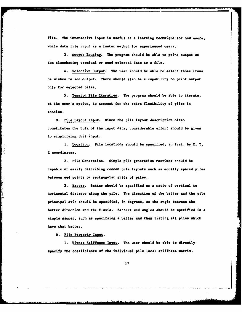
file. The interactive input is useful as a learning technique for new users,
while data file input is a faster method for experienced users.
3. Output Routing. The program should be able to print output at
the timesharing terminal or send selected data to a file.
4. Selective Output. The user should be able to select those items
he wishes to see output. There should also be a capability to print output
only for selected piles.
5. Tension Pile Iteration. The program should be able to iterate,
at the user's option, to account for the extra flexibility of piles in
tension.
C. Pile Layout Input. Since the pile layout description often
constitutes the bulk of the input data, considerable effort should be given
to simplifying this input.
1. Location. Pile locations should be specified, in feet, by X, Y,
Z coordinates.
2. Pile Generation. Simple pile generation routines should be
capable of easily describing cmon pile layouts such as equally spaced piles
between end points or rectangular grids of piles.
3. Batter. Batter should be specified as a ratio of vertical to
horizontal distance along the pile. The direction of the batter and the pile
principal axis should be specified, in degrees, as the angle between the
batter direction and the X-axis. Batters and angles should be specified in a
simple manner, such as specifying a batter and then listing all piles which
have that batter.
D. Pile Property Input.
1. Direct Stiffness Input. The user should be able to directly
specify the coefficients of the individual pile local stiffness matrix.
17
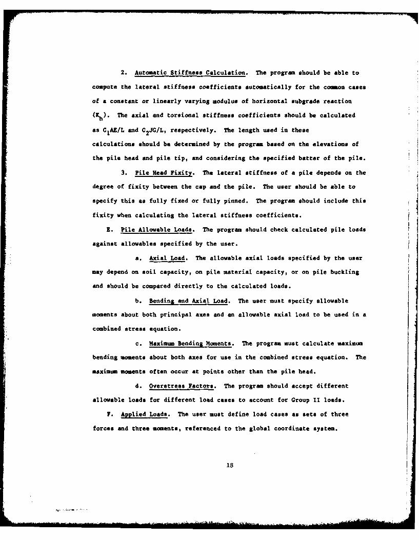
2. Automatic Stiffness Calculation. The program should be able to
compute the lateral stiffness coefficients automatically for the common cases
of a constant or linearly varying modulus of horizontal subgrade reaction
(Kh). The axial and torsional stiffness coefficients should be calculated
as C1AE/L and C2JG/L, respectively. The length used in these
calculations should be determined by the program based on the elevations of
the pile head and pile tip, and considering the specified batter of the pile.
3. Pile Read Fixity. The lateral stiffness of a pile depends on the
degree of fixity between the cap and the pile. The user should be able to
specify this as fully fixed or fully pinned. The program should include this
fixity when calculating the lateral stiffness coefficients.
E. Pile Allowable Loads. The program should check calculated pile loads
against allowables specified by the user.
a. Axial Load. The allowable axial loads specified by the user
may depend on soil capacity, on pile material capacity, or on pile buckling
and should be compared directly to the calculated loads.
b. Bending and Axial Load. The user must specify allowable
moments about both principal axes and an allowable axial load to be used in a
combined stress equation.
c. Maximum Bending Moments. The program must calculate maximum
bending moments about both axes for use in the combined stress equation. The
maximum moments often occur at points other than the pile head.
d. Overstress Factors. The program should accept different
allowable loads for different load cases to account for Group II loads.
F. Applied Loads. The user must define load cases as sets of three
forces and three moments, referenced to the global coordinate system.
18

G. Output. The program should output, at the user's option, echoes of
the pile locations, orientations, properties, and allowable loads; tables of
calculated pile forces and combined stress factors for all piles, for
selected piles, or for overstressed piles; and deflections of the pile cap
and any specified points in space.
H. Pre-Processors and Post-Processors.
1. Individual Pile Behavior. A program should be available to
calculate pile axial and lateral stiffnesses for any possible combination of
pile and soil properties. This program should also be able to calculate and
display the values of shear, moment, deflection and soil pressure along the
entire length of any pile for specified pile head loads.
2. Graphical Displays. A program should be available to display the
specified pile layout, including batters. It should also be able to display
calculated pile forces and combined stress factors superimposed on a pile
layout.
3. Pile Interference. A program should be available to check
clearances between specified piles with different locations, batters and
batter directions.
4. Base Slab Analysis. A post-processing program should be
available to use pile forces, transformed to global coordinates, to help
calculate shears and moments in portions of the pile cap.
V. ADVANCED METHODS OF PILE DESIGN.
A. PILEOPT Program. PILEOPT is a computer program intended to help
determine the most economical pile layout possible for a given set of applied
loads and within constraints specified by the user. It was developed by Dr.
James L. Hill, under a contract with the Corps of Engineers. The program
19

useb the same analysis method described previously to determine pile forces
for a given layout and applied loads. If the pile forces are less than the
specified allowables, the program deletes some piles from the previous layout
and reanalyzes. The program also attempts to choose the optimum batter for
each pile group. The CASE Task Group on Pile Foundations will furnish a more
detailed report on PILEOPT at some future date.
B. Flexible Base Analysis. The pile analysis method described above
assumes that the pile cap, or structure base slab, is rigid in comparison to
the stiffness of the piles. For many structures, such as U-frame lock
monoliths, this is not a valid assumption, and the flexibility of the base
slab should be considered. This requires use of large programs like SAP or
STRUDL which can represent the stiffness of the structure and the piles. The
pile element used in the rigid base method has been added to several versions
of the SAP program and to a version of STRUDL. Flexible base analyses have
already been performed for pile founded structures designed by the Corps of
Engineers. A more detailed report on flexible base analysis will be
furnished at some future date.
C. Non-Linear Analysis. One of the assumptions made in the rigid base
analysis method is that a pile can be represented by a set of linear
stiffnesses. The actual behavior of the pile-soil system may be highly
non-linear. Some existing programs are capable of non-linear analysis of a
structure which is supported by only a few piles. However, for large
structures supported by many piles, non-linear analysis is not currently
practical. A more detailed report on non-linear analysis will be furnished
at some future date.
20
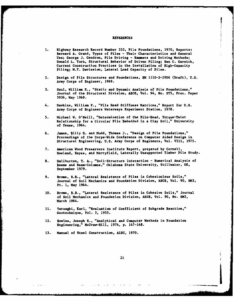
REFERENCES
1. Highway Research Record Number 333, Pile Foundations, 1970, Reports:Bernard A. Grand, Types of Piles - Their Characteristics and GeneralUse; George J. Gendron, Pile Driving - Hammers and Driving Methods;Donald L. York, Structural Behavior of Driven Piling; Ben C. Gerwich,Current Construction Practices in the Installation of High-CapacityPiling; M.T. Davission, Lateral Load Capacity of Piles.
2. Design of Pile Structures and Foundations, EM 1110-2-2906 (Draft), U.S.Army Corps of Engineer, 1969.
3. Saul, William E., "Static and Dynamic Analysis of Pile Foundations,"Journal of the Structural Division, ASCE, Vol. 94, No. ST5, Proc. Paper5936, May 1968.
4. Dawkins, William P., "Pile Head Stiffness Matrices," Report for U.S.Army Corps of Engineers Waterways Experiment Station, 1978.
5. Michael W. O'Neill, "Determination of the Pile-Head, Torque-TwistRelationship for a Circular Pile Embedded in a Clay Soil," Universityof Texas, 1964.
6. James, Billy H. and Mudd, Thomas J., "Design of Pile Foundations,"Proceedings of the Corps-Wide Conference on Computer Aided Design inStructural Engineering, U.S. Army Corps of Engineers, Vol. VIII, 1975.
7. American Wood Preservers Institute Report, prepared by Cornell,Howland, Hayes, and Merryfield, Laterally Unsupported Timber Pile Study.
8. Haliburton, T. A., "Soil-Structure Interaction - Numerical Analysis ofBeams and Beam-Columns," Oklahoma State University, Stillwater, OK,September 1979.
9. Broms, B.B., "Lateral Resistance of Piles in Cohesionless Soils,"Journal of Soil Mechanics and Foundation Division, ASCE, Vol. 90, SM3,Pt. 1, May 1964.
10. Broms, B.B., "Lateral Resistance of Piles in Cohesive Soils," Journalof Soil Mechanics and Foundation Division, ASCE, Vol. 90, No. SM2,March 1964.
11. Terzaghi, Karl, "Evaluation of Coefficient of Subgrade Reaction,"Geotechnique, Vol. 5, 1955.
12. Bowles, Joseph E., "Analytical and Computer Methods in FoundationEngineering," McGraw-Hill, 1974, p. 147-148.
13. Manual of Steel Construction, AISC, 1970.
21• I'

14. Building Code Requirements for Reinforced Concrete, ACI, 1977.
15. Recommendations for Design, Manufacture and Installation of ConcretePiles, ACI 543R, 1974.
16. Radhakrishnan, N., "Derivation of Elastic Pile Constants," unpublishedportion of lecture notes from a U. S. Army Engineer Division, LowerMississippi Valley, Pile Seminar, Jan 1976.
17. Reese, L.C. and Matlock, H., "Non-Dimensional Solutions for LaterallyLoaded Piles with Soil Modulus Assumed Proportional to Depth."
18. Mudd, T., "Supplement No. 1 5 to Letter Report, Comparative Studies forStructure Geometry and Foundation Design," Lock and Dam No. 26(Replacement) Mississippi River, Alton Illinois, St. Louis District,Corps of Engineers, February 1971.
19. Kuthy R., Ungerer, R., Renfrew, W., Hiss, F., Rizzuto, I., "LateralLoad Capacity of Vertical Pile Groups," Engineering Research andDevelopment Bureau, New York State Department of Transportation,Research Report 47.
20. Reese L. C., and Allen, J. D., "Drilled Shaft Design and ConstructionGuidelines Manual - Vol. 2 - Structural Analysis and Design for LateralLoading," U.S. Department of Transportation, Federal HighwaysAdministration, Washington, D.C., July 1977.
21. Coyle, H., and Reese, L., "Load Transfer for Axially Loaded Piles inClay," Journal of the Soil Mechanics and Foundations Division, ASCE,Vol. 92, No. SM2, Proc. Paper 4702, March 1966.
22. Coyle, H. and Sulaiman, I., "Skin Friction for Steel Piles in Sand,"Journal of the Soil Mechanics and Foundations Division, ASCE, Vol. 93,No. SM6, Proc. Paper 5590, November 1967.
23. Radhakrishnan, N., and Parker, F., Jr., "Background Theory and Documenta-tion of Five University of Texas Soil-Structure Interaction ComputerPrograms," Miscellaneous Paper WES K-75-2, Waterways Experiment Station,Vicksburg, MS, May 1975.
22

APPENDIX APILE TYPES AND ALLOWABLE STRESSES
I. GENERAL. Representative values of allowable stresses for steel, concrete
and timber piles are presented in this Appendix. This information is
compiled from data published by technical societies, voluntary standards
organizations, structural codes, and Corps of Engineers' guidance, and is
intended only for general guidance.
II. TIMBER PILES. The trees most commonly used for piles in the United
States are Douglas Fir, Southern Yellow Pine, Red Pine, and Oak. Timber
piles are generally the most economical type for light to moderate loads.
They are available in lengths from 30 to 60 ft.* Timber piles, however, are
vulnerable to damage from hard driving and to deterioration caused by decay,
insect attack, marine borer attack, and abrasive wear. Timber piles are
commonly used for dolphins and fenders for the protection of wharves and
piers because of their resilience and ease of replacement.
A. Allowable Design Stresses. Representative allowable stresses for
pressure treated round timber piles for normal load duration are shown in
TABLE A-i. These allowable stress values were derived by equations specified
by ASTM D2899. "Standard Method for Establishing Design Stresses for Round
Timber Piles". ASTM D2899 does not provide a method for establishing the
allowable tensile stress parallel to the grain. However, an allowable
tensile stress equal to the allowable bending stress may be used.
* A table of factors for converting inch-pound units of measurement to
metric (SI) units is presented on page 3.
Al
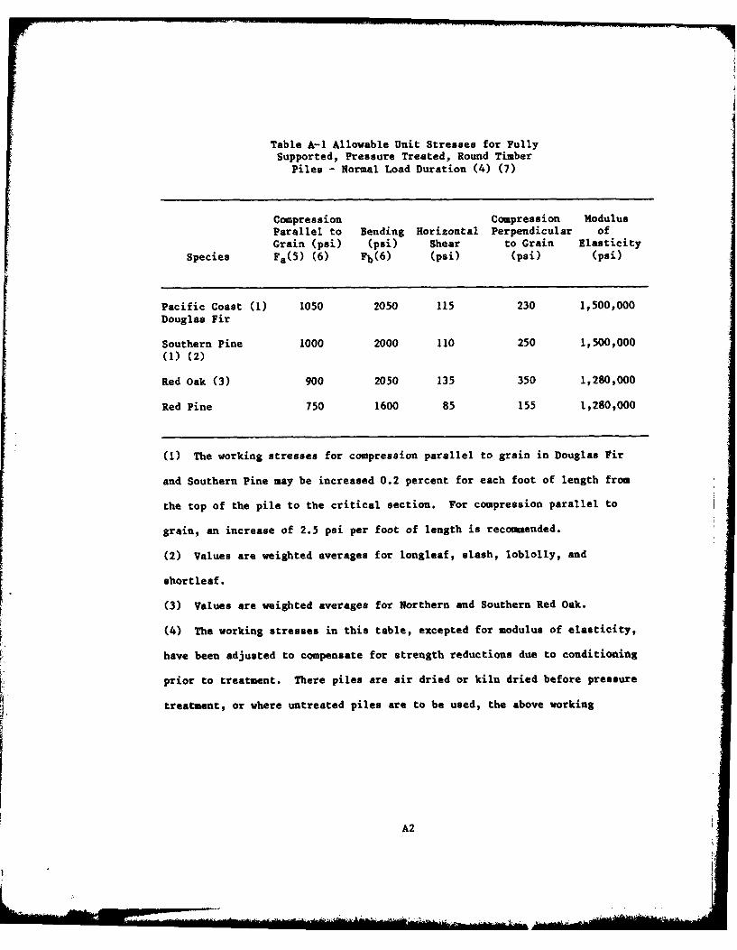
Table A-1 Allowable Unit Stresses for FullySupported, Pressure Treated, Round Timber
Piles - Normal Load Duration (4) (7)
Compression Compression ModulusParallel to Bending Horizontal Perpendicular ofGrain (psi) (psi) Shear to Grain Elasticity
Species Fa(S) (6) Fb(6) (psi) (psi) (psi)
Pacific Coast (1) 1050 2050 115 230 1,500,000Douglas Fir
Southern Pine 1000 2000 110 250 1,500,000(1) (2)
Red Oak (3) 900 2050 135 350 1,280,000
Red Pine 750 1600 85 155 1,280,000
(1) The working stresses for compression parallel to grain in Douglas Fir
and Southern Pine may be increased 0.2 percent for each foot of length from
the top of the pile to the critical section. For compression parallel to
grain, an increase of 2.5 psi per foot of length is recommended.
(2) Values are weighted averages for longleaf, slash, loblolly, and
shortleaf.
(3) Values are weighted averages for Northern and Southern Red Oak.
(4) The working stresses in this table, excepted for modulus of elasticity,
have been adjusted to compensate for strength reductions due to conditioning
prior to treatment. There piles are air dried or kiln dried before pressure
treatment, or where untreated piles are to be used, the above working
A2

stresses shall be increased by dividing the tabulated values by the following
factors:
Pacific Coast Douglas Fir, Red Oak, Red Pine: 0.90
Southern Yellow Pine: 0.85
(5) For allowable compressive stresses within the unsupported length of
timber piles, see paragraph 1.B.
(6) The allowable stresses for compression parallel to the grain and
bending, derived in accordance with ASTH D2899, are reduced by a safety
factor of 1.2 in order to comply with the general intent of paragraph 13.1 of
ASTN D2899.
(7) For hydraulic structures the values in this Table, except for modulus of
elasticity, should be reduced by dividing by a factor of 1.2. This
additional reduction recognizes the difference in loading effects between the
ASf normal load duration and the longer load duration typical of hydraulic
structures, and the uncertainties regarding strength reduction due to
conditioning processes prior to treatment.
B. Allowable Compressive Stresses for Unsupported Piles. The
allowable compressive stress for cross sections within the unsupported length
of timber piles may be determined by the formula:
F'a T - 2Z$4.0 (KL/rA)2
where:
DA
A3
- , . 1. . . .
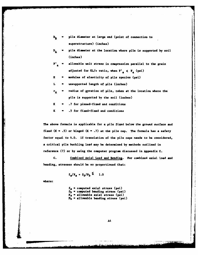
DB - pile diameter at large end (point of connection to
superstructure) (inches)
DA - pile diameter at the location where pile is supported by soil
(inches)
F' = allowable unit stress in compression parallel to the grain
adjusted for KL/r ratio, when F'a < Fa (psi)
E = modules of elasticity of pile species (psi)
L a unsupported length of pile (inches)
rA - radius of gyration of pile, taken at the location where the
pile is supported by the soil (inches)
K M .7 for pinned-fixed end conditions
K a .5 for fixed-fixed end conditions
The above formula is applicable for a pile fixed below the ground surface and
fixed (K - .5) or hinged (K - .7) at the pile cap. The formula has a safety
factor equal to 4.0. If translation of the pile caps needs to be considered,
a critical pile buckling load may be determined by methods outlined in
reference (7) or by using the computer program discussed in Appendix C.
C. Combined Axial Load and Bending. For combined axial load and
bending, stresses should be so proportioned that:
fa/ya + fb/yb l 1.0
where:
fa- computed axial stress (psi)
fb a computed bending stress (psi)Fa - allowable axial stress (psi)Fb a allowable bending stress (psi)
A4
.I .. _

The above formula is applicable for:
KL i
For KL > F , the combined axial load and bendinga '/Fa
stress should be proportional that:
fa + fb i 1.0
Fa (1-fa/fb) Fb
where:
F'a is as defined for unsupported piles
Since timber piles are tapered, the critical section or point of maxintm
stress may be at the tip for end bearing piles; or in the upper region where
subject to bending, axial load and buckling; or at some point between for
friction piles.
Il1. STEEL PILES.
Steel piles in general are available in long lengths; are able to
withstand hard driving and penetrate dense strata; and can carry moderate to
heavy loads. embedded steel piles may be subject to deterioration; by
rusting above and slightly below the ground line, especially in or near salt
water; by corrosion if the surrounding foundation material is coal, alkaline
soils, cinder fills or wastes from nines or manufacturing plants; or by local
electrolytic action.
A5
A. R Piles. H piles are nondisplacement piles which cause little
disturbance to the surrounding soil during driving. R piles can carry loads
up to 200 tons, however, the usual range is from 40 to 120 tons. Their
length, although basically unlimited, typically ranges between 40 to 100
feet. H piles are easy to splice.
B. Open-End Pipe. Open-end pipe piles can also be considered
nondisplacement piles, provided they are augered or otherwise cleaned out as
they are driven. They can be installed in unlimited lengths and can carry
moderate loads.
C. Closed-End Pipe. Closed-end pipe piles are displacement piles used
when it is desirable to add volume to and compact the surrounding soil in
order to increase the skin friction on the pile. This type of pile may cause
heave of the surrounding piles and soil.
D. Allowable Design Stresses. Allowable design stresses for steel
piles are shown in TABLE A-2. Allowable compressive stresses are given for
both the lower and upper regions of the pile. Since the lower region of the
pile is subject to damage during driving, the allowable compressive stress
should be .28 Fy (10,000) psi. This value may be increased for pipe piles
that are inspected for damage after driving. Sending and buckling effects
are usually minimal in the lower region of the pile and need not be
considered. The upper region of the pile may be subject to the effects of
bending and buckling as well as axial load. Since this region (from about 15
feet below the ground surface to the pile cap) is not usually damaged during
driving, a higher allowable compressive stress is permitted. The upper
region of the pile is actually designed in the same manner as a steel column,
with due consideration to lateral support conditions and combined stresses.
A6
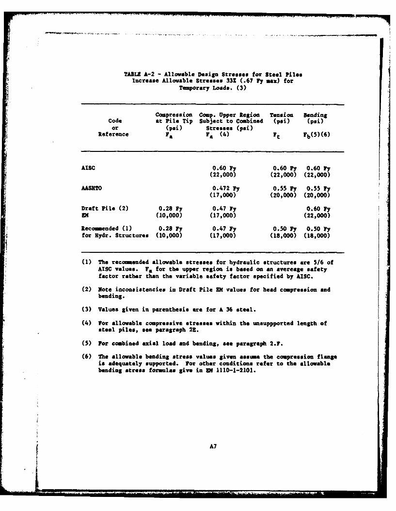
TABLE A-2 - Allowable Design Stresses for Steel PilesIncrease Allowable Stresses 33% (.67 Fy max) for
Temporary Loads. (3)
Compression Coup. Upper Region Tension BendingCode at Pile Tip Subject to Combined (psi) (psi)or (psi) Stresses (psi)
Reference 1a 1a (4) It Fb(5)(6)
AISC 0.60 Wy 0.60 Fy 0.60 Wy(22,000) (22,000) (22,000)
AASHTO 0.472 Fy 0.55 Fy 0.55 Wy(17,000) (20,000) (20,000)
Draft Pile (2) 0.28 Fy 0.47 Py 0.60 FyEN (10,000) (17,000) (22,000)
Recoummended (1) 0.28 Fy 0.47 Fy 0.50 Fy 0.50 Fyfor Hydr. Structures (10,000) (17,000) (18,000) (18,000)
(1) The recomended allowable stresses for hydraulic structures are 5/6 ofAISC values. Fa for the upper region is based on an avereage safetyfactor rather than the variable safety factor specified by AISC.
(2) Note inconsistencies in Draft Pile EN values for head compression andbending.
(3) Values given in parenthesis are for A 36 steel.
(4) For allowable compressive stresses within the unsuppported length ofsteel piles, see paragraph 21.
(5) For combined axial load and bending, see paragraph 2.F.
(6) The allowable bending stress values given assume the compression flangeis adequately supported. For other conditions refer to the allowablebending stress formulas give in EN 1110-1-2101.
A7* 4
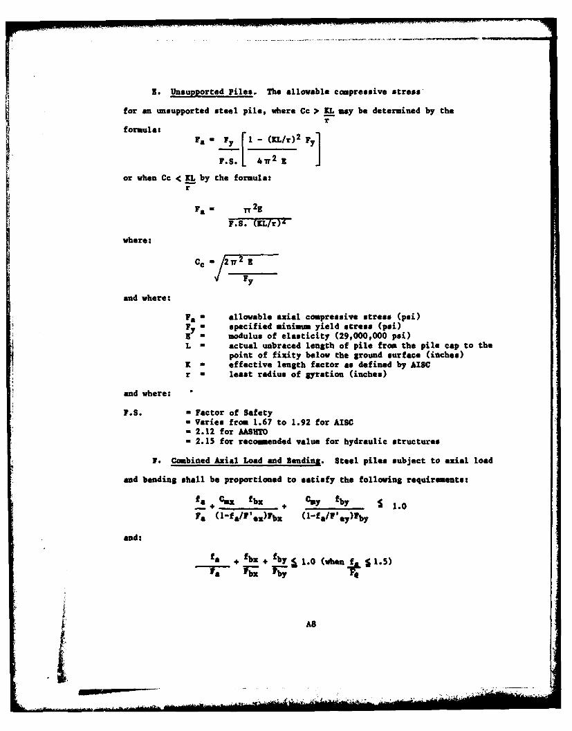
Z. Unsupported Piles. The allowable compressive stress,
for an unsupported steel pile, where Cc > KL may be determined by the
formula:F&- y[ - MK/r02 Py
F. [i 471.2 Z
or when Cc < IL by the formula:r
Fa TT 2Z
F.S. (KL/r)Z'
where:
C 27T2 Z
and where:
Fa allowable axial compressive stress (psi)-y specified minim yield stress (psi)
9 modulus of elasticity (29,000,000 psi)L - actual unbraced length of pile from the pile cap to the
point of fixity below the ground surface (inches)K - effective length factor as defined by AISCr - least radius of gyration (inches)
and where:
F.S. - factor of Safety- Varies from 1.67 to 1.92 for AISC-2.12 for MIURTO
- 2.15 for recomended value for hydraulic structures
F. Combined Axial Load and Sending. Steel piles subject to axial load
and bending shall be proportioned to satisfy the following requirements:
a. Cmx fbz + Coy tb 1.0
?a (1f/'e)b ( 1 -fa/"GY)%y
and:
AS

where:
F' 2E
e F.S.(K Lb/rb) 2
and:
fa computed axial stress (psi)
fbx or fby = computed compressive bending stressabout the x axis and y axis, respectively(psi)
Fa = allowable axial stress (psi)
Fbx or Fby = allowable compressive bending stressabout
the x and y axis, respectively (psi)E = modulus of elasticity (29,000,000 psi)
Lb = actual unbraced length of pile in the planeof bending (inches)
Kb - effective length factor as defined by AISCin the plane of bending (inches)
rb = radius of gyration in the plane of bending(inches)
C,,'or Cy coefficient about x and y axes,respectively, as defined by AISC
F.S. - Factor of Safety (see paragraph E)
G. Splices. Splices should be designed to develop the full strength
of the pile in compression, tension, and flexure.
IV. CONCRETE FILLED STEEL PILES.
A. Open- and Closed-End Pipe. Pipe piles, both open- and closed-end,
can be filled with concrete to increase their structural load-carrying
capacity. Loads up to 300 tons can be carried with this type of pile.
B. Drilled in Caissons. Drilled in caissons are typically open-end
pipe piles of 24-inch or 30-inch diameter, drilled into rock. They can carry
loads up to 300 tons. If an N Pile core section is also used, the load
carrying capacity can be increased considerably.
C. Allowable Design Stresses. Allowable design stresses for concrete
filled steel piles should follow steel and concrete allowable stresses
specified in paragraph* III and V of this Appendix.
A9
- .-
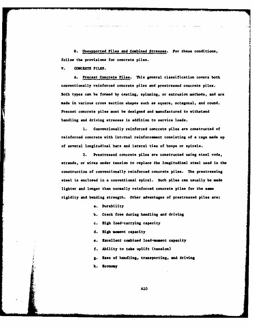
D. Unsupported Piles and Combined Stresses. For these conditions,
follow the provisions for concrete piles.
V. CONCRETE PILES.
A. Precast Concrete Piles. This general classification covers both
conventionally reinforced concrete piles and prestressed concrete piles.
Both types can be formed by casting, spinning, or extrusion methods, and are
made in various cross section shapes such as square, octagonal, and round.
Precast concrete piles must be designed and manufactured to withstand
handling and driving stresses in addition to service loads.
1. Conventionally reinforced concrete piles are constructed of
reinforced concrete with internal reinforcement consisting of a cage made up
of several longitudinal bars and lateral ties of hoops or spirals.
2. Prestressed concrete piles are constructed using steel rods,
strands, or wires under tension to replace the longitudinal steel used in the
construction of conventionally reinforced concrete piles. The prestressing
steel is enclosed in a conventional spiral. Such piles can usually be made
lighter and longer than normally reinforced concrete piles for the same
rigidity and bending strength. Other advantages of prestressed piles are:
a. Durability
b. Crack free during handling and driving
c. High load-carrying capacity
d. High moment capacity
e. Excellent combined load-moment capacity
f. Ability to take uplift (tension)
S. Ease of handling, transporting, and driving
h. Economy
AID

i. Ability to take hard driving and to penetrate
hard strata
j. High column strength
k. Readily spliced and connected
B. Cast-in-Place Concrete Piles. In general, cast-in- place concrete
piles are installed by placing concrete in a preformed hole in the ground to
the required depth. Depending on foundation conditions, the hole is usually
lined with a steel casing which is left in place or may be pulled as concrete
is placed. Since the concrete is not subjected to driving stresses, only the
stress from service loads need be considered in the design. Basic types
include the following: Cased driven shell, drilled-in-caisson,
dropped-in-shell, uncased, compacted, auger grouted injected,
cast-in-drilled-hole, and composite concrete piles. Detailed descriptions of
each of these types are covered in Chapter I of Reference 1.
C. Allowable Design Stresses. The allowable design stresses
determined in accordance with the recmmended formulas in this section relate
to the structural capacity of the pile with an applied factor of safety. The
design stresses reflect a minimum safety factor of 2.2 (based on strength
design) and include an accidental eccentricity factor of 5 percent.
Allowable design stresses for concrete piles are shown in TABLE A4. For bond
and shear allowables, see the provisions of ACI 318-77.
All

TABLE A-3 - Allowable Design Stresses for Concrete Piles
Allowable Stresses* (psi)
Permanent Loads Hydraulic Structures
ConcreteCompression
Confined** .40 fc .35 flcUnconfined .33 f'c .33 f'c
TensionPlain and Reinforced 0 0Prestressed 3 'c- (250 max) 3 /-i (250 max)
Bending CompressionAll Types .45 f'c .35 f'c
Bending TensionPlain 0 0Reinforced 0 0Prestressed 3 J (250 max) 3 /?- (250 max)
Reinforcing SteelGrade 40, 50 20,000 20,000Grade 60 24,000 20,000
*Reduce allowable stresses 10% for trestle piles and for piles
supporting piers, docks, and other marine structures.
**Provided the steel shell confining the concrete is not greater than
seventeen inches in diameter; is fourteen gage (U.S. Standard) orthicker; is seamless or has spirally welded seams; has a yieldstrength of 30,000 psi or greater; is not exposed to a detrimentalcorrosive environment; and is not designed to carry a portion ofthe pile working load.
D. Combined Axial Load and Bending. For combined axial load and
bending, the concrete stresses should be so proportioned that:
1. Axial compression and bending:
For all piles: fa + fbI 1.0
For prestressed piles: fa + fb + fpc 1 0.45 f'c(.35 f'c for hydraulicstructures, coiopression)fa - fb + fpc 0 (tension)
A12

-'
2. Axial tension and bending:
For prestressed piles: - fa - fb + fpc 0
where:
fa - actual axial stressfb - actual bending stressfpc - effective prestress after lossesI& - allowable axial stress*Fb - allowable bending stress
3. When the pile is designed for combined axial load and bending,
the working stress design should be checked using strength design methods to
insure that the required minimum factor of safety is achieved in accordance
with ACI 318-77.
E. Allowable Design Loads.
1. Laterally Supported Piles. The allowable compressive design
loads on laterally supported concrete piles may be determined by using Table
A-4.
2. Unsupported Piles. Where the pile extends above the ground or
where scour is expected, the allowable load must be reduced. For /r ratios
up to 120, the allowable load for the unsupported pile length may be
determined by applying a reduction factor R, to the allowable load for a
fully supported pile, where R - 1.23 - 0.008 (l/r) - 1.0. If 1/r exceeds
120, the pile should be investigated for elastic stability. The effective
pile length (1) is determined by multiplying the structural pile length (L)
by the appropriate value of the coefficient K listed below:
VALUES FOR K FOR VARIOUS HEAD AND END CONDITIONS
Read End ConditionsCondition
Both fixed One fixed Both hinged
Non-translating 0.6 0.8 1.0
A13
F. Other Considerations.
The pile foundation design should include other considerations to
ensure that piles are installed satisfactorily. Some of these considerations
are as follows:
1. Pile Dimensions. It is recomended that the minimum
dimension be 10 inches.
2. Pile Shells. Pile shells or casing should be of
adequate stength and thickness to withstand the driving stresses and maintain
the cross section of the driven pile.
A14
APPENDIX BPILE INSTALLATION METHODS
I. DRIVING BY IMPACT METHODS.
Most piles are installed by driving with impact hammers. These hammers
are usually powered by stem, air, or diesel. The pile driving equipment
used should be adequate to satisfactorily install the pile to the penetration
or resistance required without damage to the pile. Haner types can be
classified as gravity or drop hammers, single acting hammers, double acting
ham ers, or diesel hammers. Gravity or drop hammers are seldom used. They
consist of a weight lifted by cable to a specified height. The weight is
released and the energy, supplied by gravity, drives the pile. The single
acting hammer operates in the same fashion, only the weight is raised by
steam or air power. The steam or air power permits the weight to be raised
and released much more rapidly than by drop hammer. Double acting steam
hammers employ steam or air power to raise the hammer and to power the hammer
on the downward stroke. Diesel pile hammers get their energy from the
compression blow of a falling weight and the reaction to controlled
instantaneous burning and expansion of fuel, which raises the hammer for the
next stroke. In general, the more driving energy delivered to the pile,
without damaging the pile, the better.
II. PRE-EXCAVATION METHODS.
Pre-excavation methods such as jetting, preboring, augering, or
spudding are used when piling must be driven through dense or hard materials
to bearing at greater depth or when it is necessary to remove an equivalent
amount of non-compressible soil before installing displacement piles such as
closed-end pipe, concrete, or timber. Pre-excavation methods will also
Bi
minimize or eliminate the vibration caused by driving which may damage
adjacent structures. Pre-excavation methods should be used with care in
order to insure the desired capacity of the piles being installed and the
capacity of the piles already in place; and to insure the safety of nearby
existing structures.
A. Jetting. Jetting is accomplished by pumping water through pipes
attached to the side of the pile as it is driven. This method is used to
install piles through cohesionless soil materials to greater depths. The
flow of water reduces skin friction along the sides of the pile. Air jetting
is also used. The pile is usually jetted to within a few feet from the final
elevation and then driven. Since jetting reduces skin friction, it should be
used with caution, especially for tension piles.
B. Predrilling or Augering. Predrilling is used to produce a hole
into which a driven pile may be installed. The hole may be used to penetrate
difficult materials or to provide accurate location and alinement of the pile.
C. Spudding. Spudding is accomplished by driving a heavy pipe
section, mandrel or H pile section to provide a hole through difficult or
hard foundation materials. The spud is pulled and the pile is inserted in
the hole and driven to the required resistance.
III. VIBRATORS.
A. Low Frequency Vibrators. Low frequency vibrators deliver their
energy by lifting the pile and driving it downward on each cycle. These
operate at frequencies of 5 to 35 cycles per second. The vibration tends to
reduce the frictional grip of the soil on the pile and the pile itself is
used to impact the soil and overcome point resistance. This method has found
only limited use in driving displacement piles. Use in the installation of
nondisplacement piles, however, is increasing.
B2
-ALA

B. High-Frequency Vibrators. High frequency vibrators operate at the
natural frequency of the pile. The pile itself imparts energy to displace
the soil in front of the pile tip. High frequency vibrators operate between
40 and 140 cycles per second. Displacement piles over 100 feet long have
been installed using this method.
IV. CAST-IN-PLACE PILES.
This method consists of forming a hole in the soil and filling it with
concrete. Cast-in-place piles may be cased or uncased. Casings (shells) may
be driven with or without a mandrel. The casings are driven to the desired
resistance and filled with concrete or the casing may be slowly withdrawn as
the concrete is poured into the hole.
B3
APPENDIX C
PILE STIFFNESS COEFFICIENTS
I. GENERAL.
The ability of a pile foundation to resist applied loads depends on the
complex interaction of the pile with the surrounding soil. The numerous
factors which affect the response of a pile foundation must be reduced to a
mathematical representation so that a reasonably accurate analytical
evaluation can be performed. The most common method of accomplishing this
representation is to replace the soil and pile with springs at the
pile-structure interface. Once the various properties of the soil-pile
foundation are represented by equivalent spring constants, it is relatively
easy to determine the pile forces by use of any of several computer programs
currently available. The difficulty arises in establishing the equivalent
soil-pile springs with a reasonable degree of accuracy. Two approaches are
generally used:
- Pile load test values: determined by actual full scale pile load
tests at the construction site or a nearby site with similar soil conditions.
- Semi-Empirical: determined in two ways, by formulae or by computer
solution. If the soil modulus* can be assumed to be constant or to vary
linearly with depth, the equivalent springs can be determined directly by
formulae shown in Table C-2. For sore complex soil systems, a computer
solution can be used to account for multi-layered soils, non-linear variation
of soil modulus, and inelastic soil behavior by analyzing a single, isolated
pile using known soil parameters for the site.
*NOTE In this Appendix Ia refers to the horizontal soil modulus.
Cl
-~I.&MMA-
The equivalent springs or stiffness coefficients, determined by the
methods described above are the "b" terms of the pile stiffness matrix as
described in paragraph III D2 of the text. Generally, these terms can be
defined as:
b ij a C1IC 2
where C1 is a constant which depends on the fixity of the pile head to the
structure. For most applications, a fixity condition of fully pinned or
fully fixed is assumed. C2 is a constant based on the pile-soil
interaction and is determined by one of the methods mentioned above.
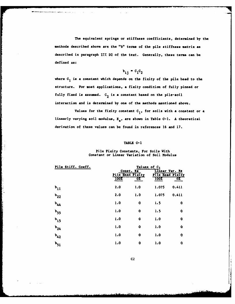
Values for the fixity constant C1 , for soils with a constant or a
linearly varying soil modulus, E., are shown in Table C-1. A theoretical
derivation of these values can be found in references 16 and 17.
TABLE C-I
Pile Fixity Constants, For Soils WithConstant or Linear Variation of Soil Modulus
Pile Stiff. Coeff. Values of C lConst. Es Linear Var. Es
Pile Head Fixitj Pile Head Fixity100% Oz IOOZ O%
b 2.0 1.0 1.075 0.411
b 2.0 1.0 1.075 0.411
b 1.0 0 1.5 044
b55 1.0 0 1.5 0
b15 1.0 0 1.0 0
b124 1.0 0 1.0 0
b42 1.0 0 1.0 0
b51 1.0 0 1.0 0
C2
.,~---..--
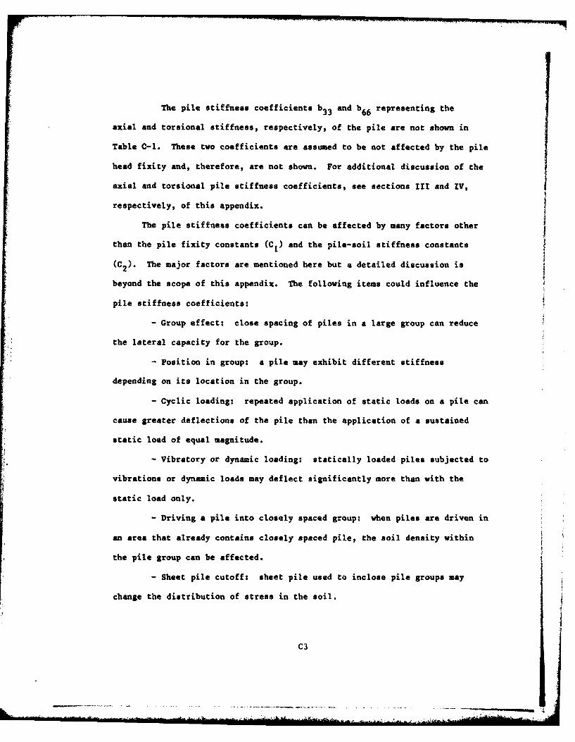
The pile stiffness coefficients b33 and b66 representing the
axial and torsional stiffness, respectively, of the pile are not shown in
Table C-1. These two coefficients are assumed to be not affected by the pile
head fixity and, therefore, are not shown. For additional discussion of the
axial and torsional pile stiffness coefficients, see sections III and IV,
respectively, of this appendix.
The pile stiffness coefficients can be affected by many factors other
than the pile fixity constants (C1) and the pile-soil stiffness constants
(C2). The major factors are mentioned here but a detailed discussion is
beyond the scope of this appendix. The following items could influence the
pile stiffness coefficients:
- Group effect: close spacing of piles in a large group can reduce
the lateral capacity for the group.
- Position in group: a pile may exhibit different stiffness
depending on its location in the group.
- Cyclic loading: repeated application of static loads on a pile can
cause greater deflections of the pile than the application of a sustained
static load of equal magnitude.
- Vibratory or dynamic loading: statically loaded piles subjected to
vibrations or dynamic loads may deflect significantly more than with the
static load only.
- Driving a pile into closely spaced group: when piles are driven in
an area that already contains closely spaced pile, the soil density within
the pile group can be affected.
- Sheet pile cutoff: sheet pile used to inclose pile groups may
change the distribution of stress in the soil.
C3
I I l li "... .... ... ... , ........... .
- Water table and seepage: the groundwater table and seepage can
influence the lateral soil modulus.
- Pile length: short rigid piles act differently than long flexible
piles. This report assumes piles are long enough to act in a flexural mode
(non-dimensional length L/T is greater than 5, as defined by Reese (17)).
- Stiffness of pile cap: the flexibility of the pile cap will
influence the distribution of load to the piles.
For additional discussion of the factors mentioned above, see reference
18.
The remainder of this appendix will deal with determination of the pile
stiffness constants (C2 ) without regard to the items briefly referred to
above.
II. LATERAL STIFFNESS.
A. General. For structures which experience lateral loads of any
significance, the correct representation of the lateral stiffness of the
foundation in the anlysis is critical. This representation must include the
resistance of the pile to lateral translation and rotation and the coupling
effects. These stiffnesses are inserted in the pile stiffness matrix as the
terms bl1, b22 , b 44 , b55 , b 15 , b24 , b4 2, and b5 1 . These
terms can be determined either by pile load tests or by semi-empirical
methods.
B. Pile Load Tests. The pile stiffness coefficients can be determined
by full scale pile load tests at the construction site or a nearby site with
similar soil conditions. However, pile load tests may not be practical for
design for several reasons:
C4
1. The tests are usually very costly and time consuming and may
not be economically feasible for small to medium size jobs.
2. Normally, pile load tests at the construction site are not
conducted until construction is yell underway. Since pile analysis and
design must be accomplished well in advance of construction, data obtained
from load tests could not be used for design but only for verification or
modification of the pile design.
3. With restricted site areas, the pile load tests can be in the
way of other construction and, in some instances, actually delay construction.
C. Semi-Empirical Methods. These methods can be categorized as
analytical (using formulae) or as numerical (using a computer solution
1. Analytical Method. If a soil system can reasonably be assumed
to have a soil modulus that varies linearly with depth or that is constant,
then the lateral stiffness constants can be calculated using prescribed
values or ranges of values of the soil modulus. Shown in Table C-2 are
formulae for calculating the lateral stiffness terms (b11 and b22 ), the
rotational stiffness terms (b44 and b55), and the coupling stiffness
terms (b15 , b24, b4 2, b51).
These terms are defined as:
b is the force required to displace the pile head a unit11
distance along the local I axis
b 22 is the force required to displace the pile head a unit
distance along the local 2 axis
b 33 is the force required to displace the pile head a unit
distance along the local 3 axis
C5

b is the moment required to displace the pile head a unit
rotation along the local 1 axis
b5 5 is the moment required to displace the pile head a unit
rotation along the local 2 axis
*b1 5 is the force along the local 1 axis caused by a unit rotation
of the pile head around the local 2 axis
*b24 is the force along the local 2 axis caused by a unit rotation
of the pile head around the local 1 axis
*bs1 is the moment around the local 2 axis caused by a unit
displacement of the pile head along the local I axis
*b4 2 is the moment around the local 1 axis caused by a unit
displacement of the pile head along the local 2 axis
*Since the stiffness matrix must be symmetric b15 b51 and
b24 = b4 2 . The sign of b24 and b42 must be negative.
TABLE C-2PILE STIFFNESS COEFFICIENTS
Pile Stiff. Coeff. Constant Es Lin. Var. Es
bl, _ _c E__ I ,--._
b22 C Es C 1 EIs.
b44 Cj --- 91.C _3
b15 C_ C, .F,.
2
C6
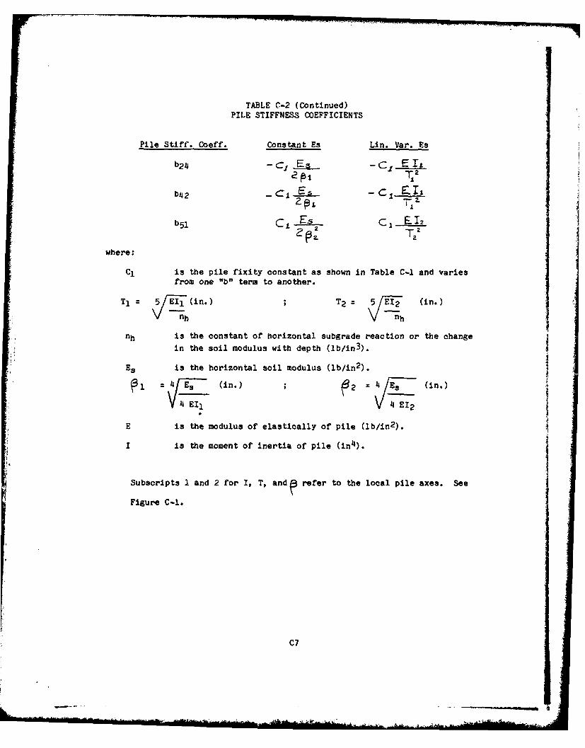
TABLE C-2 (Continued)PILE STIFFNESS COEFFICIENTS
Pile Stiff. Coeff. Constant Es Lin. Var. Es
b2 4 -C E 1T2
bL 5.1 C1 E.12
where:
C1 is the pile fixity constant as shown in Table C-i and variesfrom one "b" term to another.
Ti- 5 El (in.) T2 = 5 /E 2 (in.)
V nh V "nh
nh is the constant of horizontal subgrade reaction or the changein the soil modulus with depth (lb/in 3).
Es is the horizontal soil modulus (lb/in2 ).
S 4 FE, (in.) 2 1 L,_ (in.)j
V 4 ElI 4 E12
E is the modulus of elastically of pile (lb/in2 ).
I is the moment of inertia of pile (in4 ).
Subscripts I and 2 for I, T, andn refer to the local pile axes. See
Figure C-1.
C7

LOCAL PILE AXIS
local axis I
:a"
-_I
P axis I
local axis 2
FIGURE C-1
The constant of horizontal subgrade reaction (nh) or the horizontal
soil modulus (Zs) can be obtained using methods shown in Appendix D. These
methods are based on work by Terzaghi (19),Bron., and others and include
corrections for pile group effect and for cyclic loading. These methods of
soil modulus are satisfactory if the variation of the soil modulus with depth
can be reasonably approximated as constant or linear. Many foundation strata
fall in this category (12, 17) and can be conservatively represented by using
a "bracket" approach to the pile design. This means the pile foundation is
analyzed with weak pile stiffness coefficients and strong pile stiffness
C8
............
coefficients, where "weak" and "strong" refer to the range of soil modulus
that could reasonably be expected for a particular soil. in cases where the
simplified assumptions are not valid, computer solutions, are needed.
2. Numerical Solution by Computer. Most analytical methods are
based on a pile-soil systam similar to a bem on elastic foundation. These
methods assume that the soil can be represented by a series of closely
spaced, independent springs. The pile-soil relationship can be expressed by
a 4th order differential equation which can be solved for specific cases by
making certain assumptions. There are several computer programs available
which can be used to determine the pile stiffness coefficients for a single
pile. Some of the most useful programs are discussed in the following
paragraphs.
a. "Pile Head Stiffness Matrices." This program was written by
Dr. William Dawkins for WiE. This program is intended to be used to analyze
a single pile to determine the stiffness coefficients for input to a general
pile foundation analysis program. The procedure used is a one-dimensional
analysis of a beam on an elastic foundation where the soil is represented as
discrete springs. The soil springs are calculated by the program based on a
variation of the lateral soil modulus of E. M a + bzn.
where: iE - lateral soil modulusa, b a constantsz - depth below ground surface
The values of "a", "b", "z", and "n" are input by the user. Any degree of
fixity for the pile head to the pile cap can be considered with this
program. Output consists of the actual pile stiffness coefficients ("b"
terms) and may be used directly as input to a general pile foundation
analysis program. Disadvantages of this program are that the user must know
C9
the variation of soil modulus with depth and that the soil springs used are
linearly elastic. Also the current version of the program does not contain
provisions for variation of the pile stiffness with depth or for the
application of axial loads. For information on this program see reference 4.
b. "Analysis of Laterally Loaded Piles by Computer". Several
programs are available which can be used to determine the pile stiffness
coefficients if the values of the soil springs can be determined by other
means. The values for the soil springs are input to the program and the
springs are treated as completely elastic or elastic-plastic, depending on
the program's capabilities. Any variation of the soil modulus with depth can
be represented by inputting the proper values for the discrete soil springs.
Axial loads and variation of pile stiffness with depth can generally be
accounted for in these programs. Output usually consists of values for the
deflection, moment, and soil reaction for specified increments along the pile
model. The pile stiffness coefficients ("b" terms) can be obtained by
applying displacements and rotations to the pile model and then using the
output of forces, moments, and displacements to deterdtine the appropriate "b"
terms. For example, to determine ll" , which is the force requred to
displace the pile head a unit distance along axis 1, apply a force at the
pile head along axis 1. Then "b 1 " is equal to the displacement of the
pile head divided by the applied force. The other "b" terms can be
calculated in similar manner.
It should be noted that when the soil response to applied loads is
non-linear (as it is assumed to be in this discussion) the pile head moments
and displacements will vary non-linearly with the forces applied to the
pile. For exmple, if the applied lateral force along the pile axis 1 is
Cdo

increased linearly, the pile displacements will increase non-linearly and
therefore'%ll"will not be a constant but will vary. In order to account for
this non-linearity, the designer should determine the sensitivity of the
particular foundation to variations in applied pile loads. This can be
accomplished by comparing results from the application of small and large
loads in the single pile analysis. If the foundation is determined to be
sensitive to the load variations then the designer could account for this in
the analysis by using a bracket approach for the "b" terms or by determining
one set of "b" terms which reflect expected applied pile loads.
One of the more useful single pile analysis computer programs is
"Analysis of Laterally Loaded Piles by Computer," written by Dr. Lymon
Reese. For this program, soil properties are defined by a set of curves
which give soil reaction as a function of pile deflection. The lateral
resistance of the soil is represented by non-linear, discrete springs called
p-y curves. These curves have been constructed for various soil conditions
based on pile tests, theories for the behavior of soil under stress, and
failure mechanisms for pile-soil systems. The program performs an iterative
solution which consists of finding a set of elastic deflections of the pile
which simultaneously satisfy the specified non-linear, resistance-deformation
relations (p-y curves) of the soil and the elastic bending properties of the
pile. This program can account for changes in pile types with depth; applied
axial loads; a layered i non-linear, soil system; and any degree of fixity of
the pile head to the structure. The p-y curves are a necessary input to this
program.
Cili
Another program, "Generation of Soil Resistance versus Pile
Movement Curves," is available which will generate the required family of p-y
curves for a particular type of soil. Input to this program consists of
several parameters such as pile diameter, soil stress-strain relationship,
unit weight of soil, internal friction angle if sand or cohesion if clay, and
relative density if sand or consistency if clay. Once the p-y curves are
determined and input into the pile analysis program, the pile stiffness
coefficients can be determined from the output. The output is in the form of
pile deflection and moment, soil modulus, and soil reaction values as a
function of depth along the pile. The only major disadvantage of this
program is that the user must calculate the pile stiffness coefficients from
the output. The lateral stiffness coefficients, bll and b22, may be
calculated using applied loads and pile head displacements (computer output);
and the coupling coefficients, b42 and b5 1, may likewise be calculated
using the displacements and moments. Since the stiffness matrix must be
symetric, b42 b24 and b1 5 - b5 1. The calculation of the
rotational stiffness coefficients, b4 and b55, is accomplished by
specifying a slope (rotation) at the top of the pile and then using this
slope and the outputted moments to determine b4 and b55. Dr. Reese's
programs have been adapted for the Corps' timesharing library. For
documentation of these programs see reference 23. For an example using these
programs to determine the pile stiffness coefficients, see the sample problem
at the end of this appendix.
E. Summary and Recommendations. Calculation of the lateral pile
stiffness coefficients for use in a pile foundation analysis can be
accomplished by using data from pile load tests or by mathematically
C12

analysing a single pile. If soil parameters are not well defined, a
"bracket" approach should be used for the analytical method to account for
the numerous unknowns and assumptions involved. Results from the analysis of
a single pile using one of the computer programs discussed can be used to
verify the validity of the upper and lover limits of the "bracket". Another
approach when soil parameters are sufficiently defined through testing, is to
develop a set of stiffness coefficients for the anticipated loads using one
of the programs discussed and then use these coefficients for the pile
foundation analysis. In any case, where large numbers of pile are used or
the subsurface conditions are out of the ordinary, analytical assumptions and
results should be verified and/or modified by actual pile load tests.
III. AXIAL STIFFNESS.
A. General. The axial stiffness of a pile depends on many factors
such as the modulus of elasticity of the pile, the pile area, the pile
length, the pile tip deflection, the distribution of axial skin friction
along the pile, and the percentage of axial load transmitted to the tip.
Many of these factors are greatly affected by other related items such as
type of pile hammer, level of the water table, soil density, etc. Some of
the factors mentioned above, such as the pile length, area, and modulus of
elasticity are easily determined while some of the others are more difficult
to ascertain.
B. Tip Deflection and Distribution of Axial Forces Along the Pile.
The pile tip deflection under load and the manner in which the axial force in
the pile is transmitted to soil are interrelated and can have a great effect
on the axial stiffness of the pile. Research has indicated (21 and 22) that
the amount of load resisted by skin friction along the pile is dependent on
C13

the amount of pile tip deflection. Predicting pile tip deflection accurately
is very uncertain. Most of the group pile analyses to date have assumed
that, for compressive loads, pile tip deflection under service loads is
negligible. For this assumption, the axial stiffness can be assumed to be
AE/L for an end bearing pile with no load resisted by skin friction and 2A3/L
for a friction pile with no end bearing load transfer. These axial
stiffnesses are analogous to column effective lengths of L and L/2. Based on
a particular load distribution between end bearing and skin friction, the
modifier for the axial stiffness could vary between one and two. It must be
emphasized that the above discussion applies to pile with compressive loads
and negligible tip deflection. Tests have shown that pile having tensile
loads are less stiff (as much as a 50 percent reduction) than piles with a
compressive load. Furthermore, deflection of the pile tip of a relatively
small mount can cause the axial stiffness to be significantly different.
Additional research needs to be done to more definitely predict the axial
pile stiffness for piles with tip deflection. In the absence of better data,
the values for axial pile stiffness shown in Table C-3 have been used by some
designers.
A computer program developed by Drs. Lymon Reese and R.N. Coyle can
be used to compute load-displacement relationships for axially loaded piles.
The load transfer curves used in the program to relate skin friction to the
axial displacement of the pile are based on semi-empirical criteria. For
more information on this program see reference 23.
C14

TABLE C-3
AXIAL PILE STIFFNESS COEFFICIENTS(Assuming No Tip Deflection)
Condition -3-
Compressive load, AEend bearing pileL
Compressive load, 2AEfriction pile L
IV. TORSIONAL STIFFNESS.
For a three dimensional pile group, a torsional pile constant (b66 )
can be defined which relates the rotation of the pile in a plane
perpendicular to its longitudinal axis to an applied torque. This can be
expressed as
b66 =CT JG
L
where:
CT is a constant which describes the distribution of torsionalshear to the soil and the transfer of torsional shearresistance from the pile to the structure.
J is the polar moment of inertia of the pileG is the shearing modulus of elasticityL is the length of pile
Unless the pile group is small (say less than 10 piles), the torsional
stiffness of the individual pile appears to have little effect on the
stiffness of the pile group and can be conservatively assumed to be zero.
C15
EXAMPLE PROBLEM:
ANALYSIS OF SINGLE PILE TO DETERMINE PILE STIFFNESS COEFFICIENTS
C16

Determine the pile stiffness coefficients for the pile shown in Figure 0-2
using p-y curves to represent the lateral res istance of the soil. Asse the
pile head to be fixed to the pile cap.
#/~ST P Y~OPT A
- I YMEDIUM4 SAND
0 z35* =.61 rod. -
C2o I P P-Y #2W sub x63.5 PCF= .0367PC1
STIFF CLAY
C =576PSF a 4.0OPSII sub= 51.5 PCF x.0298 PCI
PILE 6TYPE n HP 14)(T3
E :29 x10 6 pS1 P-Y 41 261 IN4 /
I1 729 IN4 -
FIGURE C-2
j C17
STEP #1. Determine the p-y curves for the, soil strata shown in Figra C-2.
Use computer program CORP8110004 (NAIR) to generate the p-y curve data. This
program also has graphics capabilities which can be used to plot the input
data and the p-y curves. Your p-y curves are generated: one at the ground
surface, one at the bottom of the sand layer, one near the top of the clay
layer, and one at the bottom of the clay layer. The plot of the input data
f or the example is shown in Figure C-3. Figures C-4, C-5, and C-6 are plots
with different scales of the p-y curves developed by the program. Figure C-7
is a listing of the output file for the example. For a complete program
description and variable definitions see reference 23.
C18.

I-=j 3o4-0j
0 fa F
awo9-WC -&Ol & .W
o1
6A.-.

IL-
LL)*~
02
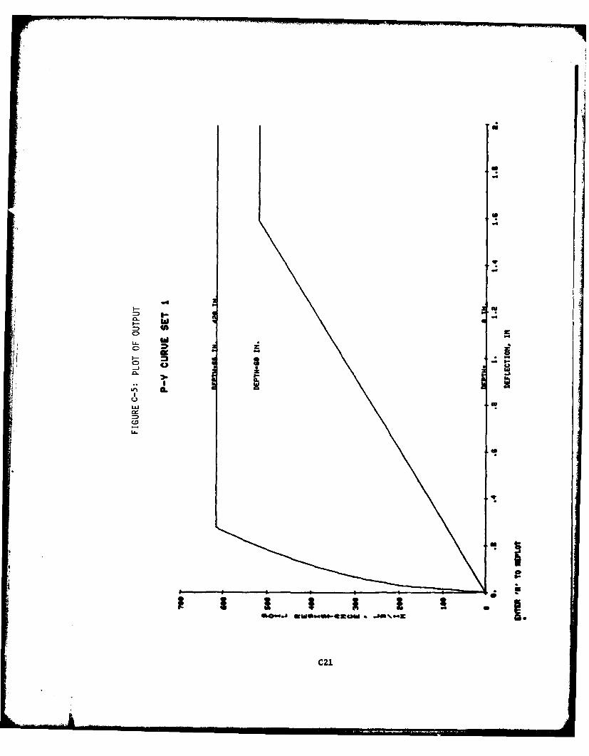
4
CD.
I- I-
93.4II-
I, LL
LL.
S 'C21

CL1
C)I
LLNI
9L-
ti
C2
6MS. .
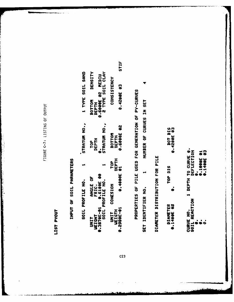
0> > I
w aa z0 WC 0 M 6-I.- IU - h h
0- IL 00
V4 -0.0L
06 4
0 (AZ Z "s
I- 010 0 w- 0 AM
F- E l 00 Z cc hW I. W i-i-. 0 6-0
4~LL 00 4 "LI i ~OCLi I- I= c 0 so
OW V4 0 *L w CLw a
04 0 0 a LL. a hihiL
0. w0 - CL s- 1.-Sai ..4 0 0 hi. 0.hihi w "4W " 0 0 0- sL a0 a Zam 0 ZW.C LL hi hi W 1-00V4
L. a 0L .1 0.W4 ~ ~ * W -
0. 0o WO 0 Q. 0 & -a. a xU 0 CL I-- I- C>h
hi P4 4~h 1 4 0" 11 0 0 a 0w c
> 8. 0 00=s - h I - cI0 a 911 =wo 1- IV (
"4 (A :pZO Z-ob M. V4 4000
=WM~ cu I- 4 M
C23

u cu P')0 0 0
* 0a c
a* 0 000000 0 000000*O- W 04 111" I
o .. 0 **.*Q@ 0W O*096*6000000
mu1 - 000000 m e00000
z Mt MMzMM ~ MMMM~
o s0 00 00000 0 00000000000Il- WW 11- WWWWWWWWWWW F- wIAWWWWWWWWW
.0 WIV *0 0g~n~q 0 0 MWVWWWVOVOO04 00 0C CCUI-~W 04~WUWD
w 030 ZW wW'UC'44Za
=0 .J400 .I******~.o~o**
00b 0G (A C
C24
STEP #2. Once the p-y curves are determined, the force-displacement data for
the curves are used to represent the soil behavior and are input to a program
to analyze a single, laterally-loaded pile. For this analysis use program
CORPS/IO001 (COM62). An additional p-y curve (#0) has been added at the top
of the pile. This set of data merely represents the absence of soil at the
top of the pile. Program COM62 uses a linear interpolation between
succeeding p-y curves that are input. Using the p-y curves as specified
force-deformation relations for the soil and the pile flexural stiffness, the
program solves the differential equations representing the pile-soil
relationship. This is performed in an iterative fashion until the elastic
behavior of the pile matches the specified soil behavior. Four runs of
computer program COM62 are required. Two runs are required to determine the
respective pile stiffness coefficients for each principal axis of the pile.
In the first run only a lateral force is applied along pile axis 1 to the top
of the pile In the second run, a slope along the pile axis 1 is applied at
the top of the pile. The graphics associated with program COM62 give plots
of the input as well as the soil pressure, moments, and deflections for the
pile. Plots of the input data for the first two runs are shown in Figures
C-8 and C-9 and a plot of the output for the runs 1 and 2 are shown in
Figures C-10 and C-11 (respectively). A listing of selected output is shown
in Figure C-12. For a complete program description and variable definitions
see reference 23.
C25
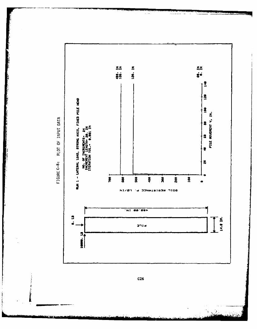
zz
U- *4 14*
WU 0 IA
10
Niles" "30
52
-C2

inC> 4
-j m I,
aI.LLa
33laS~ no
C2
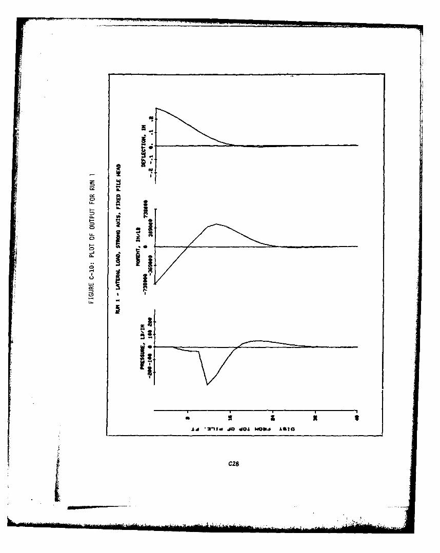
CC 4
w=
Cz
aL-
AI-no4 04Wb Lt
C2
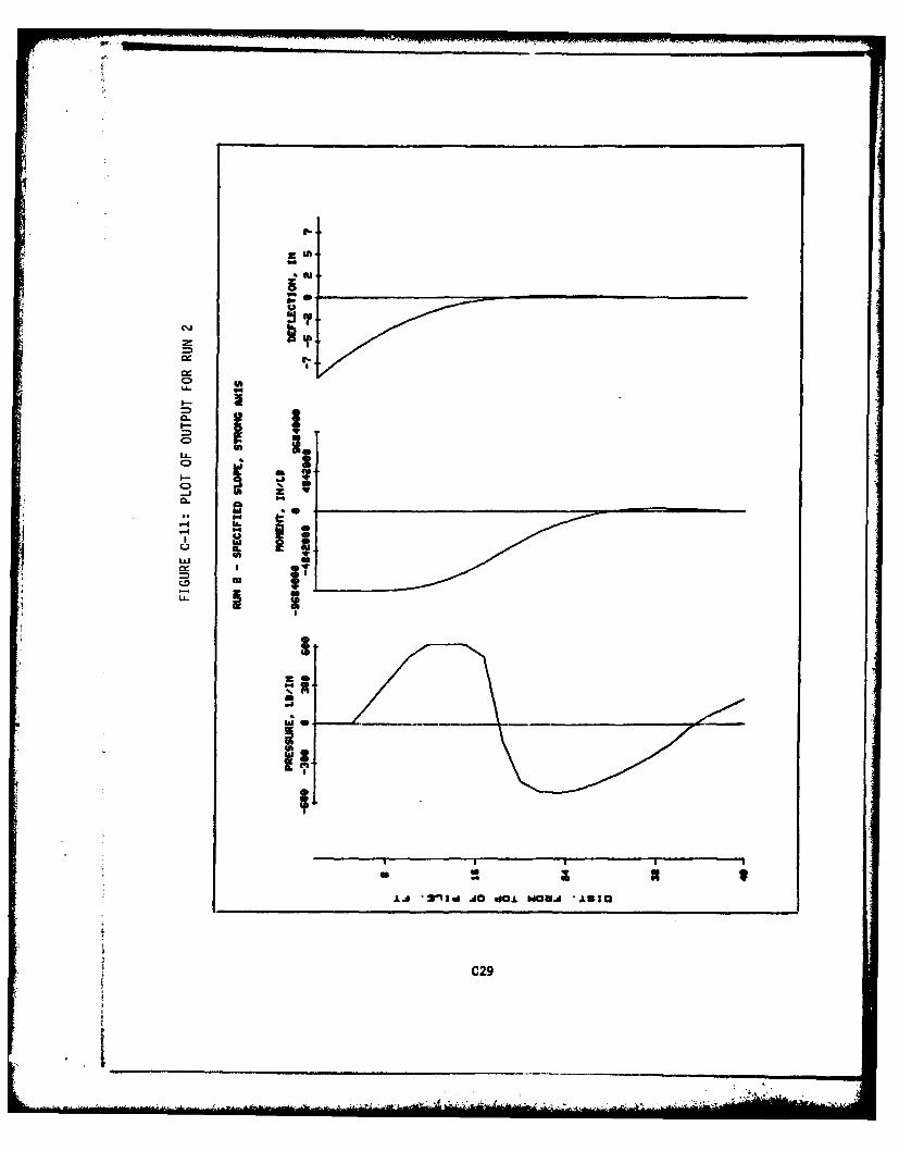
CDs
LL
C-
LL
oz
IdausS
Jo40 NN
SbC29

ime
o w4
IL "3
U * U)
Ca si
'-4z I wwww
U) 0 0 0 0
0 00
f340 we (
- I-- 6 * S *
LL
C30*
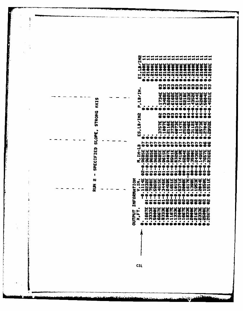
\ WWWWWWWWWWWWWWWWW
We..eee~ec
w 4 .6q q q q 4 q w 4 @ @ -@CAIW OWW WIWIatfIO~
w .@xe
a*
- -- - - 'ygwwwpuuqwqw-CA -- m
s-b t. @ OJ .'-J
z w i myqwwwwwwqw
w
IL-
cu w IWWWWWWWWWWWWWWWWW
* '4 *w~w~m1v~wU)W(~z
(U z .wwwwwwwwwwwwwwww
I.- 6- "MWUOW@1W O- IwU')mm M- - (U@44@4fl@4u
*~ ~ ~ ~~1 ** S S** S@S
C3
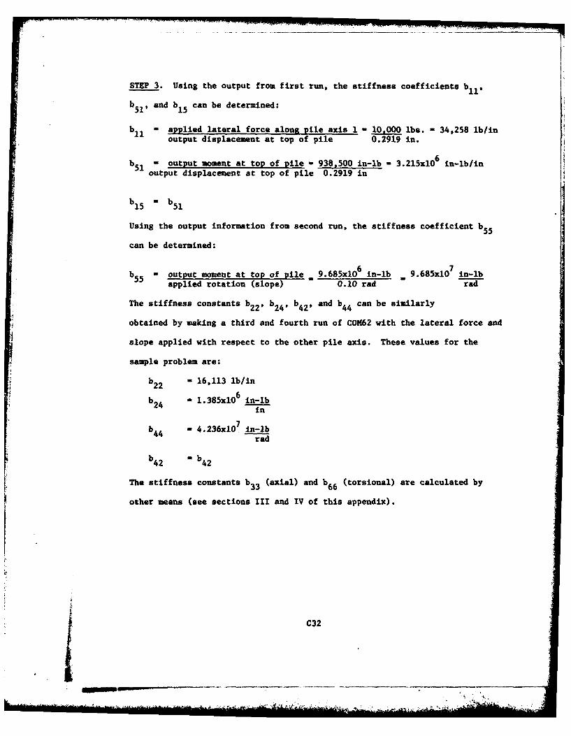
STEP 3. Using the output from first run, the stiffness coefficients bll,
b51, and b15 can be determined:
bl1 - applied lateral force along pile axis 1 10.000 lbs. - 34,258 lb/inoutput displacement at top of pile 0.2919 in.
b 510 output moment at top of pile - 938,500 in-lb - 3.215xi06 in-lb/inoutput displacement at top of pile 0.2919 in
b15 =b 51
Using the output information from second run, the stiffness coefficient b55
can be determined:
b55 - output moment at top of pile - 9.685xi06 in-lb . 9.685xi07 in-lbapplied rotation (slope) 0.10 rad rad
The stiffness constants b22, b24 , b42, and b4 4 can be similarly
obtained by making a third and fourth run of COM62 with the lateral force and
slope applied with respect to the other pile axis. These values for the
sample problem are:
b2 16,113 lb/in
6b2 1.385xi0 in-lb24 in
b44 - 4.236x10? in-lbrad
b4 2 "b 42
The stiffness constants b33 (axial) and b66 (torsional) are calculated by
other means (see sections III and IV of this appendix).
C32
APPEDIX D
SOIL HODULUS FOR LATERALLY LOADED PILES
The lateral pile stiffness coefficients discussed in Appendix C can be
directly computed when E is a constant or linearly varying in the media in
which the pile is embedded. It is generally assmed that for homogeneous
cohesive soils I is constant and for homogeneous cohesionless soils X
varies linearly with depth. In this Appendix, typical values for computing
I for homogeneous cohesive and cohesionless soils are provided. The
structural engineer must rely on the geotechnical engineer to obtain the
values of the soil modulus and the coefficient of horizontal subgrade
reaction.
Definitions and Nomenclature
Ki - Coefficient of horizontal subgrade reaction (lbs/ft3 ) (ratio ofpressure (lbs/ft2 ) at a point to the displacement (ft) at thepoint) for a 1 foot wide pile embedded in clay.
Kh - Coefficient of horizontal subgrade reaction (lbs/ft3 ) (Kb -
2K(Ift)/B(ft)).
is - Soil modulus (lbs/ft2 ) - ratio of soil resistance (p) (lbs/ft)to pile movement (y) (t), is - Ih).
nh - Constant of horizontal subgrade reaction (lbs/ft3 ) for a pile 1foot wide embedded in sand (Kh - nZ/, Be - nh).
I - Width of pile (ft).
Z - Depth below ground surface (ft).
qu - Unconfined compressive strength of clay (Ibs/ft2 ).
I & R2 - Reduction factors
1 - Unit weight of soil
D1
Romopeneous Soils
If the soil is homogeneous and can be classified as clay (cohesive)
or sand (cohesionless), estimates of S can be computed using values
developed by Terxaghi (11), Broms (9, 10), and others based on experiments
and theoretical relations. The range of values provided by these authors
(see next sections) must be reduced for cyclic and group effects on piles.
It should be noted that these values are based on the assumption that the
soil has linear elastic properties. The values are only valid for simple
soil conditions and sust be used with caution.
Cohesive Soils
For cohesive soils Z is assmed to be constant with depth.
m - s,(1)
- "I (lft/) (2)
The value of K1 can be estimated by using the relation,
K1 - a(80%) (3)
where a is a parameter on a 1 foot strip that varies from 0.32 to 0.52
(Reference 10, 20), generally use a - 0.4 (ft-).
qu is the unconfined compression strength of clay in lbs/ft2.
Thus,
K1 - 0.4(80%) - 32% (4)
Therefore, 1h - 3 (5)
Note that the units of Kh are in lbs/ft3 with qu being in lbs/ft and
4 1 in feet.
D2
*1~~ __ ___

-32qu (6)
Note that the units of 16in the above equation are the sae as those of
Reduction Factors
The values obtained for I~ must be reduced to account for the effects of
cyclic loading (R) and group action (R2). Thus,
Use R1 1 for initial loading and - 0.3 for cyclic loading (References 9,
10). The value of R2 can be obtained froma Table D-1 (Reference 1) given
below.
TAIL D-1
Values of Group Effect Factor (122
Pile Spacing in
R1 Direction of Loading
1.00 SD0.*85 7D0.70 6D0.55 5D0.40 4D0.*25 3D
Cohessionleasse Soils
in cohesionless soils, due to confinement effects, a 9 inceases with depth.
It is generally assumed that this variation is linear.
Is , nZ(8)
when nh is the constant of horizontal subgrade reaction and Z is the depth
below equivalent ground surface.
D3
-. . ----- e i
Teruaghi (Reference 11) provided the following empirical relation for
obtaining nh:
nh A__ (9)
1.35
where A is a value obtained as a function of the relative density of soil as
shown in Table D-2 and J is the effective unit weight of sand. The units of
A will be the same as those of 3.
TABLE D-2
Values of A as a Function of the Relative Density of Sand
Relative Density N* Value of A
Loose 4- 10 100- 300
Medium 10 - 30 300 - 1000
Dense 30 - 50 1000 - 2000
*l is the number of blows of the drop weight required to drive the samplingspoon into the soil for a distance of one foot. A weight of 140 lbs and aheight of fall of 30 inches are considered standard.
The value I is the effective unit weight of the sand. If the piles are below
the water table, the submerged unit weight of the sand should be used in
computing the value of nh . If the piles extend above the below the water
table, an equivalent height of submerged sand should be developed above the
water table. The depth Z then must be measured from the top of the
equivalent ground surface. Thus,
D4
,~J
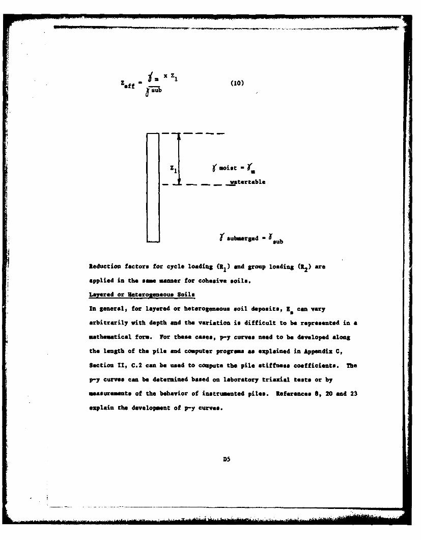
Zeff = xZ 1 (10)
zij -~moistm
...atertable
submersed =
Reduction factors for cycle loading (R and group loading (R2) are
applied in the same manner for cohesive soils.
Layered or Ieterogeneous Soils
In general, for layered or heterogeneous soil deposits, ts can vary
arbitrarily with depth and the variation is difficult to be represented in a
mathematical form. For these cases, p-y curves need to be developed along
the length of the pile and computer programs as explained in Appendix C,
Section 11, C.2 can be used to compute the pile stiffness coefficients. The
p-y curves can be determined based on laboratory triaxial tests or by
measurements of the behavior of instruoiented piles. References 8, 20 and 23
explain the development of p-y curves.
D5
73

For homogeneous layered soils that are cohesive or cohesionless, the
appropriate relations given in the preceding sections could be used. For
cohesive soils, the values are only dependent on the unconfined
compressive strength of each of the layers. For cohesionless soils, the E.
values are dependent on nh for the layer and the effective depth (Zeff)
The effective depth is calculated for each layer as shown:
Zeff
Z2 [t2 ~zf - Z (1z1
3
Summary
Typical values for are given for homogeneous cohesive and cohesionless
soils. It must be emphasized that the pile lateral stiffness coefficients
can be directly computed only when EK8 is a constant (such as for a
homogeneous cohesive soil) or linearly varying (as for homogeneous
cohesiveless soil). In all other cases including layered soils and soils
that cannot be classified as cohesive or cohesionless, the pile stiffness
coefficients can be calculated by using computer programs such as those
elaborated in Appendix C, Section 11, C.2 of this report.
D36
-~A .
APPENDIX E
EXAMPLE PROBLEMS
EXAMPLE PROBLEMS 1 THROUGH 5
Two-dimensional Problems
Hrennikoff' s Example
Comparison of Computer Output with
the Elastic Center Method
Hrennikoff's calculations and a
Common Analytical Method
Example problems 1 through 5 illustrate how the computer can be used to analyze
two-dimensional pile foundation problems. The following examples were taken
from Hrennikoff's paper entitled "Analysis of Pile Foundations with Batter Piles",
published in the Transactions of the American Society of Civil Engineers, Vol.
76, No. 1, Paper No. 2401, Jan. 1950, pp. 123-126.
The computer results are compared with Hrennikoff's results as well as with
other hand computation methods commonly used by civil engineers.
The physical pile layout for example problems 1 through 5 is shown in Figure El.
Example Problem No. 1 compares the results obtained by the Computer Method with
those obtained by the Elastic Center Method assuming the soil offers no lateral
support; in other words, the subgrade modulus is zero. The Computer results
agree closely with the Elastic Center Method results. A description of the
Elastic Center Method can be found in "Substructure Analysis and Design" by
Dr. Paul Andersen. This method is limited, however, to pile groups consisting
of hinged piles arranged in two subgroups whose centerlines intersect.
El
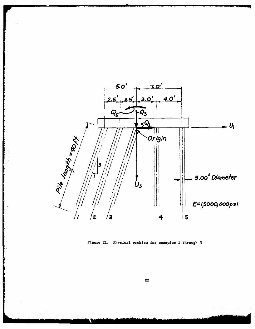
II
3.0 40- I -'
I,'F ,I,' u
Ori9in
// . 9.000 Doiame / r~~~/' /1t/ / O Oo
/Z a4 15
Figure El. Physical problem for examples 1 through 5
E2
Example Problem No. 2 compares the results obtained by the Computer Method
with the results obtained by Manual Calculations as presented in Hrennikoff's
paper for case 2a (very weak soil with a subgrade modulus of 3.123 psi). The
Computer results agree closely with Hrennikoff's calculations.
Example Problem No. 3 compares the results obtained by the Computer Method with
the results obtained by Manual Calculations as presented in Hrennikoff's paper
for Case 4a (weak soil with a subgrade modulus of 31.23 psi). The Computer
results agree closely with Hrennikoff's calculations.
Example Problem No. 4 compares the results obtained by the Computer Method with
the results obtained by Manual Calculations as presented in Hrennikoff's paper
for Case 6a (medium soil with a subgrade modulus of 312.3 psi). Again, the
Computer results agree closely with Hrennikoff's calculations.
Example Problem No. 5 compares the results obtained by the Computer Method with
the results obtained by a common Analytical Method for two different load
conditions. A description of the common Analytical Method can be found in
"Foundation Engineering" by Ralph Peck, Walter E. Hanson, and Thomas H.
Thornburn, and in "Foundation Design" by Wayne Teng. Example Problem No. 5
demonstrates that the individual pile forces obtained by the common Analytical
Method are approximate and may or may not agree closely with the results obtained
by the Computer Method. A subgrade modulus of 312 psi was used for this example.
E3

Example Problem 1
Two-dimensional problemHrennikoff's exampleno lateral soil support
Properties
E = 0.15 x 10⁷ psi Degree of fixity = 0.0
Modsu b = 0.1 Vo Pile resistance = 0.5
I = 322.06 in.4 Participation factorx for torsion = 0.0
I = 322.06 in.4 Torsion modulus = 0.0y
Area = 63.5 in.2
Length = 30 ft
Loading QI Q3 Q5Case (kips) (kips) (kip-ft)
1 -39.375 113.1 173.4
Properties and loading conditions
for example problem 1
E4

I EXAMPLE PROBLEM NO 12 HRENNIKOFF EXAMPLE3245115 1 .1
61 5 30.000 37 9.000849 1500000.00010 211 0. 1,00. O012 113 82.000 40.0001415 1 3 -3.00016 4 5 0.17 -5.000 -2.5 0. 3.000 7.00018 -39.375 113.1 173.4
E>FILESTROMS EDITED,C>REPLACED STRON5C>DLDPCORPS/UN=CECELBC>CALL PCORPSP X0034
JOB WAITING.
INPUT DATA FILE NAME IN 7 CHARACTERS OR LESS. HIT ACARRIAGE RETURN IF INPUT DATA WILL COME FROM TERMINAL.
I>STROM5
THIS PROGRAM GENERATES THE FOLLOWING TABLES:
TABLE NO. CONTENTSI PILE AND SOIL DATA2 PILE COORDINATES AND BATTER3 STIFFNESS AND FLEXIBILITY MATRICES FOR THE
STRUCTURE AND COORDINATES OF ELASTIC CENTER4 APPLIED LOADS5 STRUCTURE DEFLECTIONS6 PILE DEFLECTIONS ALONG PILE AXIS7 P1! E FORCES ALONG PILE AXISB PILE FORCES ALONG STRUCTURr AXIS
E5
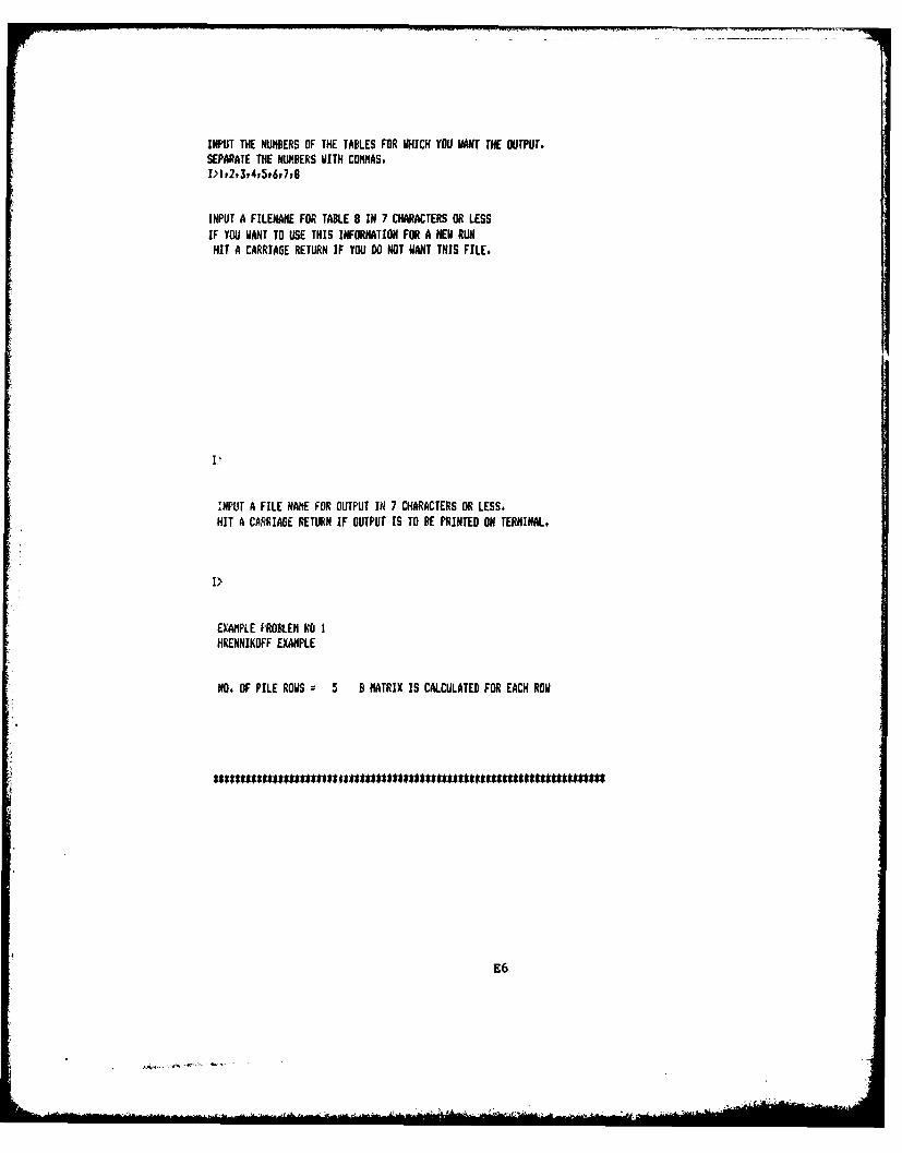
INPUT THE NUMBERS OF THE TABLES FOR WHICH YOU VANT THE OUTPUT.SEPARATE THE NMBERS WITH COMMAS.I)1.2t3r4y5t6,7,9
INPUT A FILENAME FOR TABLE 8 IN 7 CHARACTERS OR LESSIF YOU WANT TO USE THIS INFORMATION FOR A NEU RUNHIT A CARRIAGE RETURN IF YOU DO NOT WANT THIS FILE.
Vi
INPUIT A FILE NAME FOR OUTPUT IN 7 CHARACTERS OR LESS.HIT A CARRIAGE RETURN IF OUTPUT IS TO BE PRINTED ON TERMINAL,
EXAMIPLE PROBLEM NO 1HRENNIKOFF EXAMPLE
NO. OF PILE ROWS 5 B MATRIX IS CALCULATED FOR EACH RON
E6

1. TABLE OF PILE AND SOIL DATA
PILE NUMBERS
1 5 E = .15EW07 PSI IX 322.06 INl*4 IY = 322.06 IN*4AREA x 63.6 IN1st2 X 9.00 IN Y z 9.00 INLENGTH = 30.0 FEET ES .100K1 = .4107 K2 = 1.0000 K3 z 0.0000K4 z 0.0000 1(5 = 0.0000 1(6 = 0.0000
LENGTH OF PILES ( 30.00 FEET) IS INSUFFICIENTFOR PILE GROUP - 1 MINIMUM ACCEPTABLE LENGTH IS 97.88 FEETFOR SETI-INFINITE DEAN ON ELASTIC FOUNDATION
ALLOWABLES: COMPRESSIVE LOAD = 82,000 KIPSTENSILE LOAD 2 40,000 KIPS
THE B MATRIX FOR PILES I THROUGH 5 IS
.186E402 0. 0,0, ,265E+06 0,0. 0, 0,
2- i.,LL, OF PILE CWRDINATE5 AND DATIER
PILE ROM PATTER Ul (FT)1 -3.00 -5,0002 -3.00 -2.5003 -3,00 0,0004 VERTICAL 3.0005 VERTICAL 7.000
E7

3. STIFFNESS MIATRIX S FOR THE STRUCTURE
.796Ef0S -.239E406 -.716E407-.239Ef 06 .125E+07 -.103E+08-.7160 07 -.103Ef08 .329E+10
3A FLEXIBILITY MATRIX F FOR THE STRUCTURE
.127E-03 .274E-04 .363E-06,274E-04 6S7IE-015 *007E-07.363E-06 .807E-07 .135E-08
COORDINATES OF ELASTIC CENTERECI .003 EC2 -.002
ft"008 LOADING CONDITION I 00S~f
4. MATRIX OF APPLIED LOADS 0 (KIPS I FEET)
at 03 as
-39.375 113,100 173,400
ES
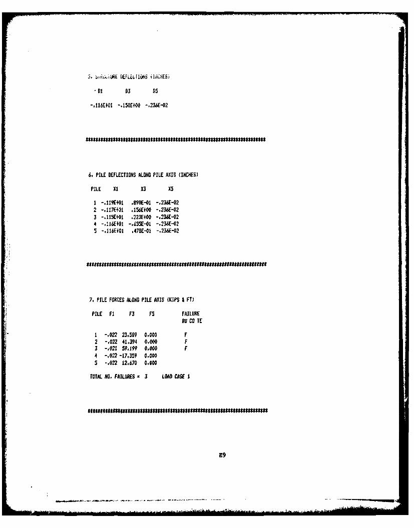
DI1 03 D5
*,116E+01 -,150E+00 -,236E-02
6. PILE DEFLECTIONS ALONG PILE AXIS (INCHES)
PILE X1 X3 X5
1 -.119E+01 .890E-01 -,236E-022 -.117E+01 .156Ef00 -*236E-023 -.115E+01 .223E+00 -.236E-024 -.!16E+01 -,655E-01 -.236E-025 -.116E#01 *478E-01 -.236E-02
7. PILE FORCES ALONG PILE AXIS (KIPS a FT)
PILE Fl F3 F5 FAILUREDU CO TE
1 -.022 23.589 0.000 F2 -.022 41.394 04000 F3 -1021 59.199 0.000 F4 -.022 -17.359 0.0005 -.022 12.670 0.000
TOTAL NO. FAILURES =3 LOAD CASE I
E9

8. PILE FORMES ALONG STRUCTURtE AXIS (KCIPS I FEET)
PILE Fl F3 F5
1 -7.481 22.371 0.0002 -13.111 39.263 0.003 -18.741 56.155 0.0004 -.022 -17.359 0.0005 -.022 12.670 0.000
-- -- -- -- -- -- -- - -- -- -- -- -- -- -- - --- -- -- -- -- ---

Analysis by elastic center method
Eiosfic 20Centec 5 .2
-Resu/ho Force - R
Localintl oF ,9es&#
1K 734 -53'
__K__-39_____75_
113.1i /~~For~e.5 reJl' "I
ollechn oplgo
Y 03
2I 3 -
1443
Ell
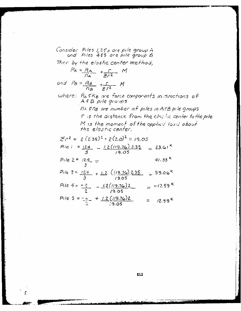
Cc e Pi5 I, 7,e I pie 91cu0 UPrG:-nd Pl,/e-5 4,,5 are pile group t3
i- -3 A +r fv
flA
~~nJ 5,~ r M
where cf'-'c or ~e CCYapPC1~,)7'5 In :%ftecr/l a ofA8 p,'le Pro vp 5rlA ,"17 Ore 1uimber- o f piles Ii,) p.i /e 9roupS
r ;s i* difonce frarm +he /c *: , ~ ~ rArep
M 0 hrnre,- of te Opp/i; tl cj o r!
7)L e/osi57'c,/r
-Z + 2-
Pile ;2 Z z~ /O9.7(.) 2.3 Z3 G 5I3 /9.05
P) /ea Z a 41.53
P/ile = g ('s&a.35 0 ~
/9.05
PIle 5=-- + /.z/59
E12
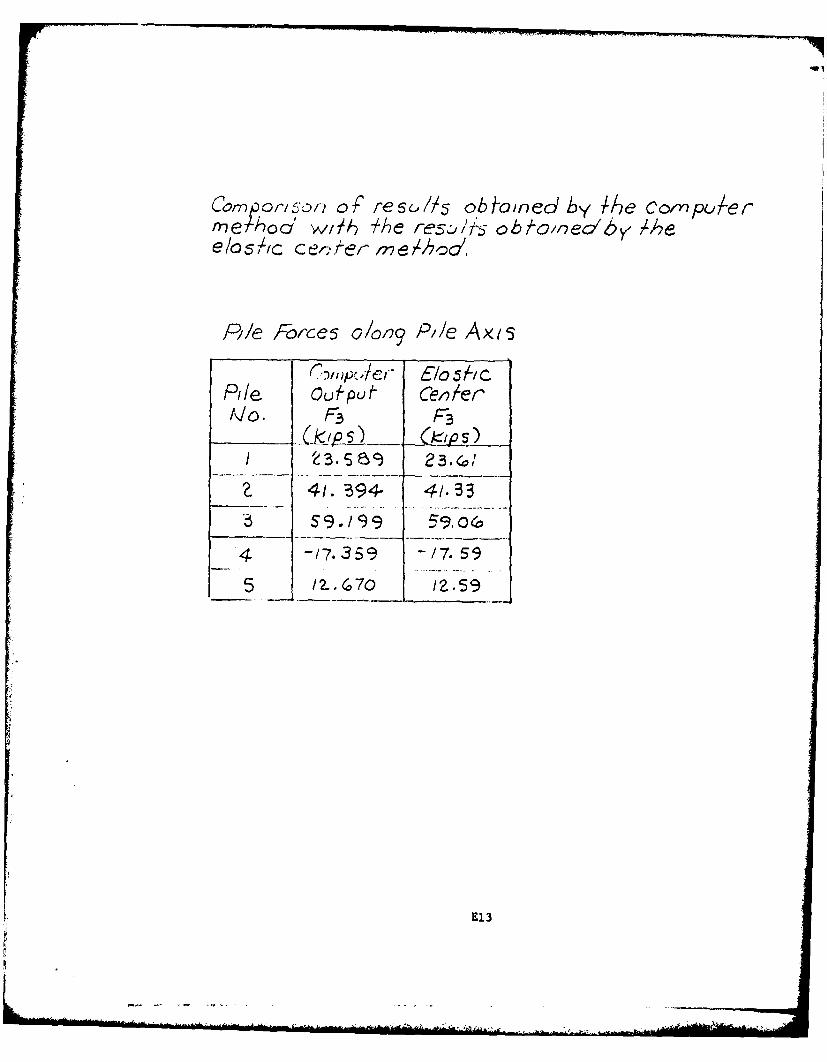
Corn p rl~oo of' resc,//5 obtolned by Me comnpc/-ermne hoc' \,v//6 The re~sob/-oloecQb, 4hee/o s -I ce Ine e 7 heoa'
Pl/e Forces c/ol'9 P1/e Axis
Pil/e ou&pfr Ce7ter/'J3.FF
~3. (o
S9./99 59. o
_4 -/7-359 -/7.59
E13

Example Problem 2
Two-dimensional problem,Hrennikoff's examplecase 2a (very weak soil)
Properties
E =0.15 X10 psi Degree of' fixity =0.0
Modb 3.123 psi Pile resistance =0.5
14I = 322.06 in. Participation factorfor torsion = 0.0
IY=322.06 in. Torsion modulus =0.0
Area = 63.5 i. 2
Length =30 ft
Loading Q3iQCase (kips) (kips) (kip-ft)
1-39-375 113.1 173.14
Properties and loading conditions forexample problem 2
E14
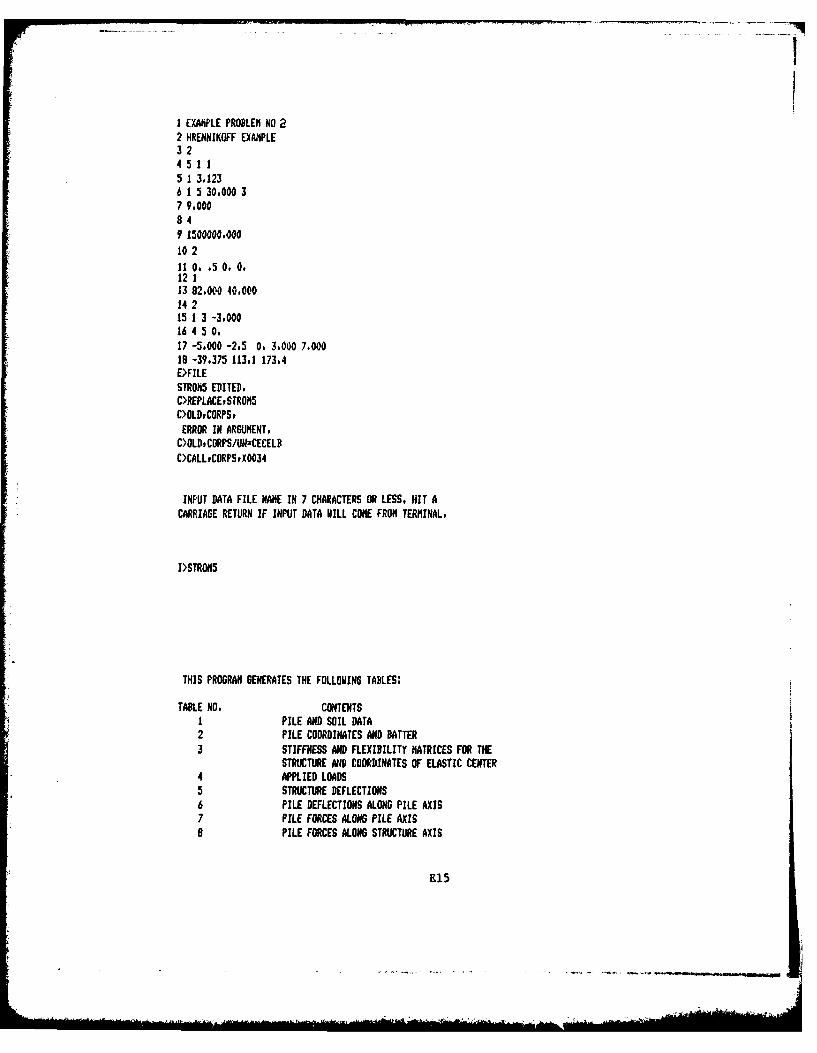
1 EXAMPLE PROBLEM NO 22 HRENNIKOFF EXAMPLE3 2
5 1 3,1236 1 5 30,000 37 9.0008 49 1500000.000
10 2
11 0. .5 0. 0.12 113 82.000 40.00014 215 1 3 -3.00016 4 5 0.17 -5.000 -2.5 0. 3.000 7.00019 -39,375 113.1 173.4E>FILESTROllS EDITED,C>REPLACErSTRON5C>0LD, CORPStERROR IN ARGUMENT,
C>0LDsCORPS/UJ=CECELBC>CALLrCORPSvXOO34
INPUT DATA FILE NAME IN 7 CHARACTERS OR LESS, HIT ACARRIAGE RETURN IF INPUT DATA MILL COME FROM TERMINAL,
I>STROI5
THIS PROGRAM GENERATES THE FOLLOWING TABLES:
TABLE NO. CONTENTS1 PILE AND SOIL DATA2 PILE COORDINATES AND BATTER3 STIFFNESS AND FLEXIBILITY MATRICES FOR THE
STRUCTURE AND COORDINATES OF ELASTIC CENTER4 APPLIED LOADS5 STRUCTURE DEFLECTIONS6 PILE DEFLECTIONS ALONG PILE AXIS7 PILE FORCES ALONG PILE AXIS0 PILE FORCES ALONG STRUCTURE AXIS
E15

INPUT THE NUMBERS OF THE TABLES FOR WHICH YOU WANT THE OUTPUT,SEPARATE THE NUMBERS WITH COMMAS.
INPUT A FILENAME FOR TABLE 8 IN 7 CHARACTERS OR LESSIF YOU WANT TO USE THIS INFORMATION FOR A NEU RUNHIT A CARIAGE RETURN IF YOU 0O NOT WANT THIS FILE.
EAA? LE PROBLEM NO 12HRENNIKOFF EXAMPLE
NO. OF PILE ROWS 5 B MATRIX IS CALCULATED FOR EACH ROW
E16

-A 093 696 ARMY ENGINEER WATERWAYS EXPERIMENT STATION VICKSBURG MS F I 13/13DEC 80 .J HARTMAN
UNCLASSIFIED WES-TR--80-5 Ht.
~~22 f1 lfflffllfllfllfmEhhEEI
W- 12.5I
11111125 1-14 ____
MICROCOPY RESOLUTION TEST CHART

1. TABLE OF PILE AND SOIL DATA
PILE NUMBERS
1 5 E = *15E+07 PS IX 322.06 IN*t4 IY = 322.06 INt$4AREA 63.6 IN$$2 X 9,00 IN Y = 9.00 INLENGTH = 30.0 FEET ES = 3.123KI = .4107 K2 = .5000 K3 = 0,0000K4 z 0.0000 K5 0.0000 K6 0.0000
LENGTH OF PILES (30.00 FEET) IS INSUFFICIENTFOR PILE GROUP - I MINIMUM ACCEPTABLE LENGTH IS 37.17 FEETFOR SEMI-INFINITE BEAN ON ELASTIC FOUNDATION
ALLOWADLES: COMPRESSIVE LOAD 82,000 KIPSTENSILE LOAD 40.000 KIPS
THE B MATRIX FOR PILES 1 THROUGH 5 IS
.246E+03 0. 0,0, .133E+06 0,0, 0. 0.
2. TABLE OF PILE COORDINATES AND BATTER
PILE ROW BATTER til (F7)1 -3,00 -5,0002 -3.00 -2.500
3 -3.00 0.000I5 VERTICAL 7,000
5 VERTIAL 7.00

3. STIFFNESS MATRIX S FOR THE STRUCTURE -
,409E#05 -.119E#06 -,357E# 07-.119Ef06 *623E+06 -*517Ef 07-.357Ef07 -.517Ef07 .164Ef 10
3A FLEXIBILITY MATRIX F FOR THE STRUCTURE
.193E-03 *414E-04 .350E-06*414E-04 ,105E-04 *123E-06.550E-06 .123E-06 .219E-08
COORDINATES OF ELASTIC CENTEREC1 .003 EC2 -.002
M*SS LOADING CONDITION I *MM:
4o MATRIX OF APPLIED LOADS 0 (KIPS I FEET)
a1 03 05
-39.375 113.100 173.400
E18
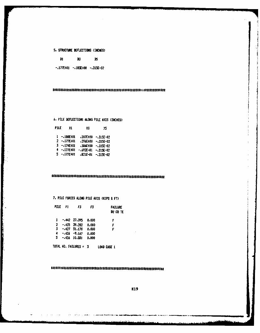
5. STRUCTURE DEFLECTIONS (INCHES)
D1 D3 D5
-. 177E+01 -. 183E400 -,315E-02
6. PILE DEFLECTIONS ALONG PILE AXIS (INCHES)
PILE Xl X3 x5
I -. IBOE01 .207E+00 -,315E-022 -.177E+01 .296E+00 -,315E-023 -.174EfOl .386E#00 -.315E-024 -.177E+01 -.692E-01 -,315E-025 -.17?E01 .821E-01 -315E-02
7. PILE FORCES ALONG PILE AXIS (KIPS I FT)
PILE Fl F3 F5 FALIRE
0U CO TE
1 -,442 27.395 0,000 F2 -.435 39.282 0.000 F3 -.427 51.170 0.000 F4 -.436 -9.167 0,0005 -.436 10.881 0,000
TOTAL NO. FAILURES 3 LOAD CASE 1
I*$Iti S*r*~tSSIrtt¢t¢g¢ssetr gsCsstssese ss¢ns nn ¢ns ¢n¢.munE1
E1l9
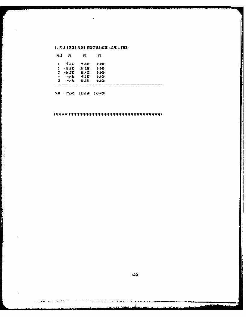
E. PILE FORCES ALONG STRUCTURE AXIS (KIPS I FEET)
PILE Fl F3 F5
1 -9.08? 25.849 0.0002 -12.935 37,129 0,000
3 -16.587 48,403 0.0004 -,436 -9,167 0.0005 -.436 10.381 0.000
SUN -39,375 113.1.4 173,400
E20
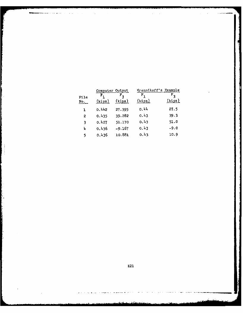
Comnuter Outnut 1renni-koff's Ex-aile
Pile F131 3
1 o.1442 27.395 o.144 27.5
2 o.2435 39.282 o.243 39.3
3 o.1427 51.170 0.143 51.0
14 0.1436 -9.167 0.143 -9.0
5 0.1436 lo.881 0.143 10.9
E2 1
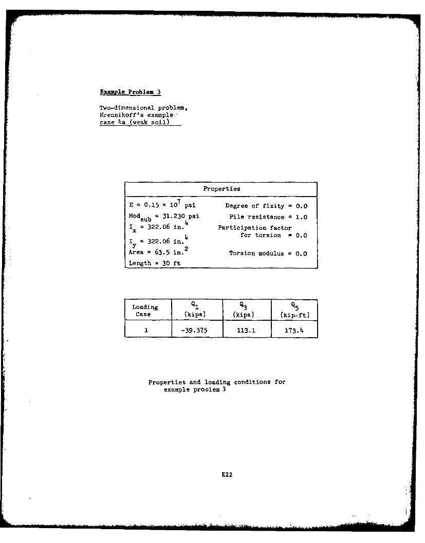
Example Problem 3
Two-dimensional. problem,lrennikoff's examplecase ha_(wealk soil)
Properties
E0.15 x 107 psi Degree of fixity = 0.0
Mdsub =31.230 4psi Pile resistance = 1.0IX = 322.06 in. Participation factor
I = 32.06 n. 4for torsion = 0.0
Area =63.5 in.2 Torsion modulus = 0.0
LLength =30 ft
Loading 3Q5Case (kips) (kips) (kip-ft)
1 -39.375 113.1 173.'4
Properties and loading conditions forexample pro olem 3
E22
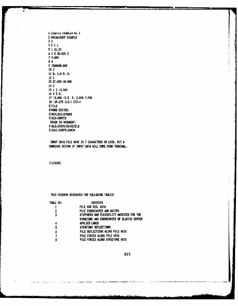
i Xek IIWBLtM N 32 HRENNIKOFF EXAVrLE3?2
7190000.0
12 4
13967.000 40.00014 215 1 3 -3.00016 4 5 0,17 -5,000 -2.5 0. 3.000 7.00018 -39.375 113.! 173.4EMILESTROMS EDITED.C>REPLACEPSTROM5C>OLDiCORPCSERROR IN ARGUMENT.
C>OLDYCORPS/UN:CECELDC>CALL ,CORPSX0034
INPUT DATA FILE NAPIE IN 7 CHARACTERS OR LESS. HIT ACARRIAGE RETURN IF INPUT DATA WILL COPE FROM TERMINAL,
I>STROM5
THIS PROGRAM GENERATES THE FOLLOWING TABLES:
TABLE NO, CONTENTS1 PILE AND SOIL DATA2 PILE COORDINATES AND BATTER3 STIFFNESS AND FLEXIBILITY MATRICES FOR THE
STRICTURE AND COORDINATES Ov ELASTIC CENTER4 APPLIED LOADS5 STRUCTURE DEFLECTIONS6 PILE DEFLECTIONS ALONG PILE AXIS7 PILE FORCES ALONG PILE AXISB PILE FORCES ALMN STRUCTURE AXIS
E23

INPUT THE NUMBERS OF THE TABLES FOR WHICH YOU WANT THE OUTPUT,
SEPARATE THE NUMBERS WITH COMAS.
INPUT A FILENAME FGR TABLE 8 IN 7 CHARACTERS OR LESSIF YOU WANT TO USE THIS INFORMATION FOR A NEW RUN
HIT A CARRIAGE RETURN IF YOU DO MD!T NANT THIS FILE,
EXAMPLE PROBLEM NO 3HRENNIKOFF EXAMPLE
NO. OF PILE ROWS 5 B MATRIX IS CALCULATED FOR EACH ROW
E24
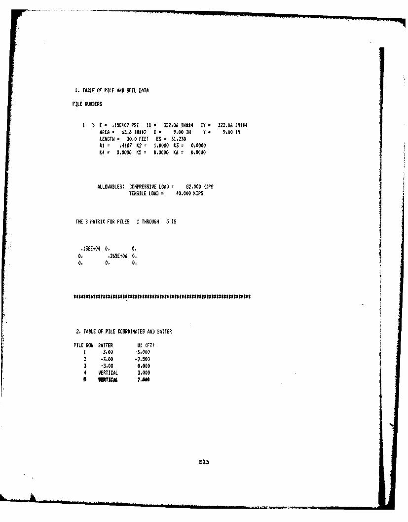
1. TABLE OF PILE AND SOIL DATA
PILE NUMBERS
1 5 E = 1SE+07 PSI IX 322.06 IN04 IY = 322.06 INZ*4AREA = 63.6 IN$*2 X 9.00 IN Y = 9.00 INLENGTH = 30,0 FEET ES = 31.230K1 = .4107 K2 = 1.0000 K3 = 0.0000K4 = 0.0000 K5 = 0.0000 K6 = 0.0000
ALLOWABLES: COMPRESSIVE LOAD = 82.000 KIPSTENSILE LOAD = 40.000 KIPS
THE B MATRIX FOR PILES 1 THROUGH 5 IS
.138E+04 0. 0.0. .265E+06 0.0. 0. 0.
2. TABLE OF PILE COORDINATES AND BATTER
PILE ROW BATTER Ul (FT)1 -3.00 -5.0002 -3.00 -2.5003 -3.00 0.0004 VERTICAL 3,0005 V1CAL 7.1
E25
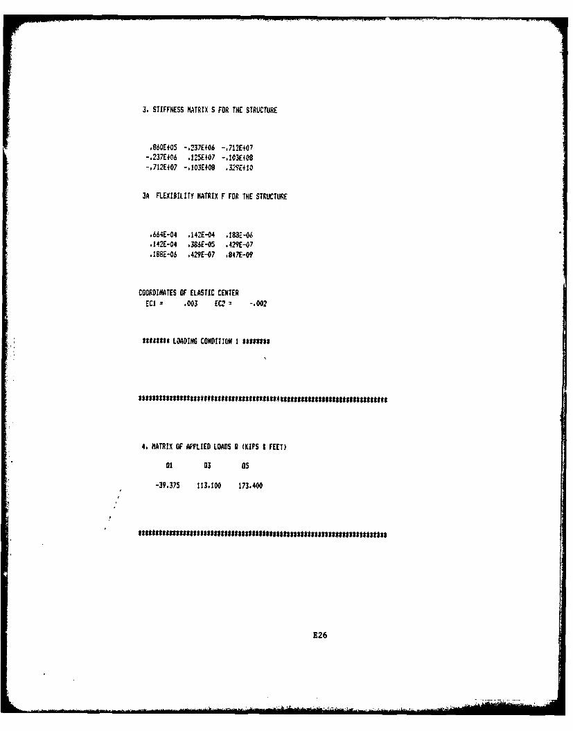
3. STIFFNESS MATRIX S FOR THE STRUCTURE
.060E+05 -.237E+ 06 -.712E407-*237E#06 .125E107 -. 103E408-,712E+07 -.I03E#08 .32S'E+1O
3A FLEXIBILITY MATRIX F FOR THE STRUCTURE
.664E-04 .142E-04 .188E-06
.142E-04 *38SE-05 .429E-07
.ISSE-06 .429E-07 .847E-09
COORDINATES OF ELASTIC CENTERECI .003 EC2 = -.002
Wt$*$* LOADING CONDITION I h8I*U$
4. MATRIX OF APPLIED LOADS A (KIPS :FEET)
al 03 05
-39,375 113.100 173.400
E26
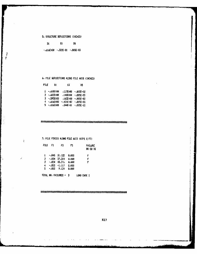
5. STRUCTURE DEFLECTIONS (INCHES)
-*616E+00 -.332E-01 -.805E-03
6. PILE DEFLECTIONS ALONG PILE AXIS (INCHES)
PILE xi X3l X5
1 -.610Ef00 .117E+00 -.BOSE-032 -.602E+00 .140E+00 -.BOSE-033 -. 595jE+00 .163E+00 -.805E-034 -.616E#00 -.421E-02 -,B05E-035 -.616E+00 .344E-01 -.805E-03
7. PILE FORCES ALONG PILE AXIS (KIPS 1. FT)
PILE Fl F3 F5 FAILUREBU CO TE
1 -.845 31.132 0,000 F2 -,834 37.2C4 0.000 F3 -.824 43.276 0.000 F4 -,853 -1,117 0,0005 -.853 9.124 0,000
TOTAL NO. FAILURES 3 LOAD CASE I
E27

8, PILE FORCES ALONG STRUCTURE AXIS (KIPS 3 FEET)
PILE Fl F3 F5
1 -10,646 29.267 0.0002 -12.556 35.031 0.0003 -14.467 40,795 0,0004 -.853 -1.117 0.0005 -.853 9-124 0.000
SUN -39,375 113.100 173.400
E28
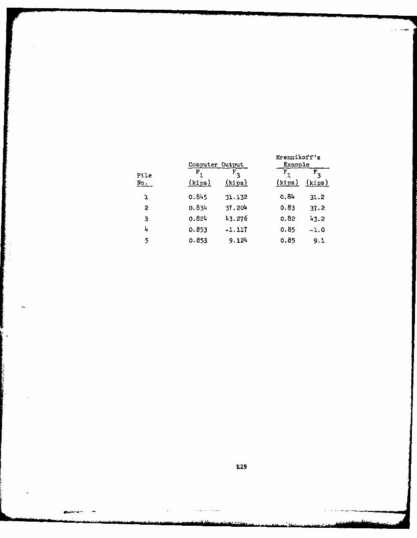
Hrennikoff'sComtuter Output Exannie
Pile F 1 F 3 F 1 F 3No. (kinps) (kinps) (ki-os) (kins)
I. o.845 31.132 o.84~ 31.2
2 o.834 37.2o14 0.83 37.2
3 0.824~ 43.276 0.82 43.2
14 0.853 -1.117 0.85 -1.0
5 0.853 9.124' 0.85 9.1.
FE29
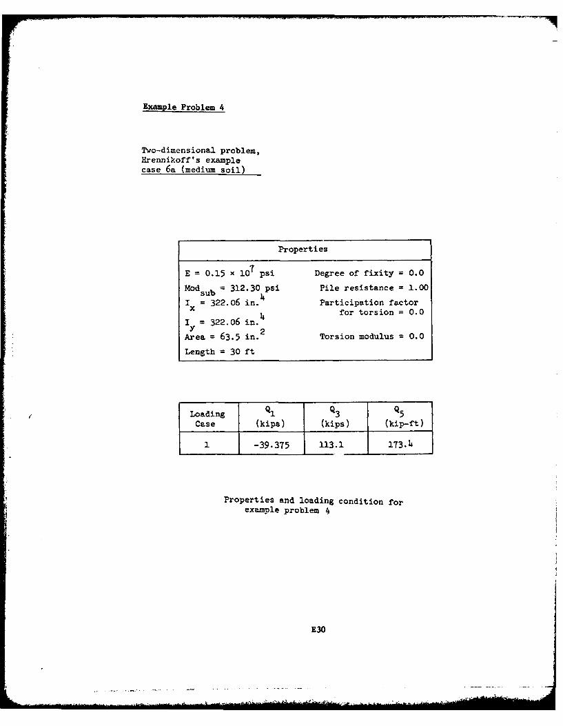
Example Problem 4
Two-dimensional problem,Hrennikoff's examplecase 6a (medium soil)
Properties
E = 0.15 x 10⁷ psi Degree of fixity = 0.0
Modsub = 312.30 psi Pile resistance = 1.00
Ix = 322.06 in. Participation factor
4 for torsion = 0.0Iy = 322.06 in.~
Area = 63.5 in.2 Torsion modulus = 0.0
Length = 30 ft
Loading Q1 l3 I 5Case (kips) (kips) (kip-ft)
1 -39.375 113.1 173.4
Properties and loading condition forexample problem 4
E30
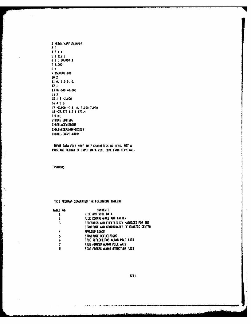
2 HRENNIKOFF EXAMPLE3245115 1 312.36 1 5 30,000 37 9.000849 1500000.00010 211 0. 10 00 0,12 113 82.000 40.00014 2151 1 -3,00016 4 5 0.17 -5,000 -2.5 0. 3.000 7.00018 -39.375 113,1 173,4F)FILESTROM5 EDITED.C>REPLACESTROM5
C>OLDPCORPS/N=CECELBC>CALLPCOPStX0034
INPUT DATA FILE NAME IN 7 CHARACTERS OR LESS. HIT ACARRIAGE RETURN IF INPUT DATA UILL COME FROM TERMINAL.
I>STRON5
THIS PROGRAM GENERATES THE FOLLOING TABLES:
TABLE NO. CONTENTS1 PILE AND SOIL DATA2 PILE COORDINATES AND BATTER
3 STIFFNESS AND FLEXIBILITY MATRICES FOR THESTRUCTURE AND COORDINATES OF ELASTIC CENTER
4 APPLIED LOADS5 STRUCTURE DEFLECTIONS6 PILE DEFLECTIONS ALONG PILE AXIS7 PILE FORCES ALONG PILE AXIS8 PILE FORCES ALONG STRUCTURE AXIS
E31
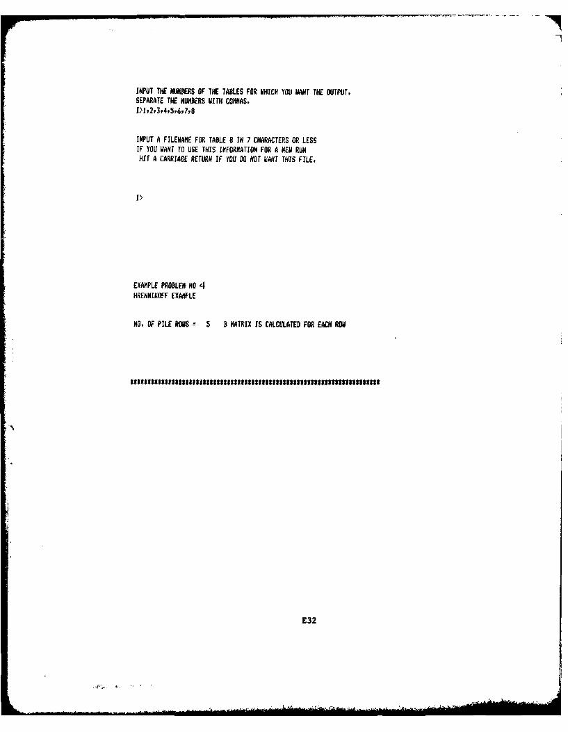
INPUT THE NUMBERS OF THE TABLES FOR WHICH YOU WIANT THE OUTPUT.SEPARATE THE NUMBERS WITH COMMAS.I)I,,2t3,4,5,6,7tB
INPUT A FILENAME FOR TABLE 8 IN 7 CHARACTERS OR LESSIF YOU WANT TO USE THIS INFORMATION FOR A NEW RUNHIT A CARRIAGE RETURN IF YOU DO NOT WANT THIS FILE,
I>
EXAMPLE PROBLEM NO 4HRENNIKOFF EXAMPLE
NO. OF PILE ROWlS 5 B MATRIX IS CALCULATED FOR EACH RON
E32
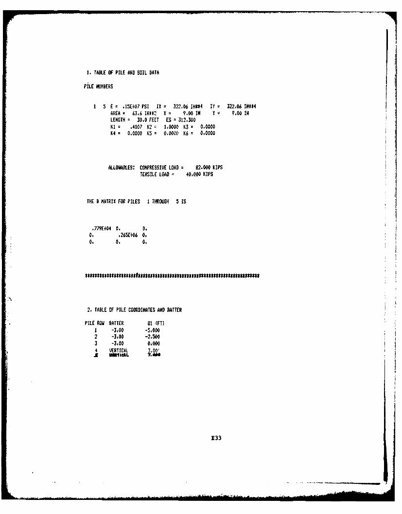
1. TABLE OF PILE AND SOIL DATA
PiLE NUMBERS
1 5 E = .15E407 PSI IX 322.06 IN*$4 IY = 322,06 INt*4AREA = 63.6 INtt2 X 9.00 IN Y = 9.00 INLENGTH = 30.0 FEET ES = 312.300K1 = .4107 K2 1.0000 K3 = 0.0000K4 = 0.0000 K5 0.0000, K6 = 0,0000
ALLOgABLES: COMPRESSIVE LOAD 82.000 KIPSTENSILE LOAD = 40,000 KIPS
THE B MATRIX FOR PILES 1 THROUGH 5 IS
.779E+04 O 0,0, .265E+06 0.0, 0. 0.
2. TABLE OF PILE COORDINATES AND BATTER
PILE ROW BATTER U! (FT)1 -3,00 -5.0002 -3.00 -2,5003 -3.00 0.0004 VERTICAL 3,00,.E VIInicAL %
E33
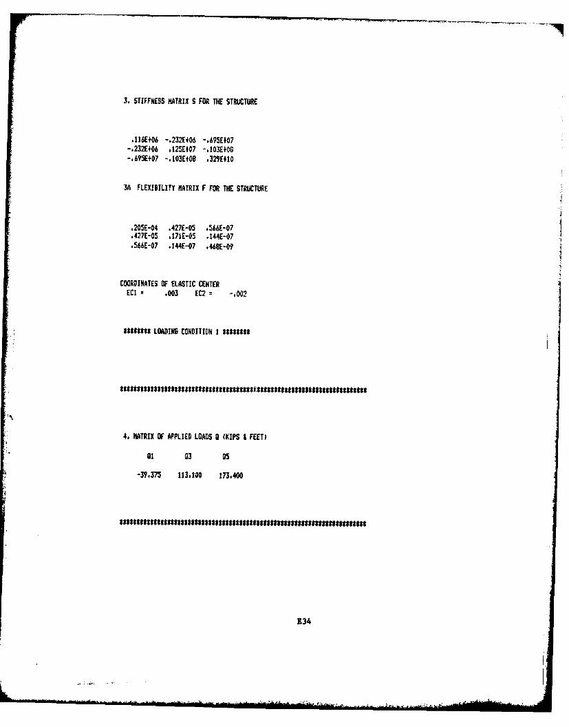
3. STIFFNESS MATRIX S FOR THE STRUCTURE
.116E+06 -.2320406 -.695E+07-.232E+06 *125E407 -.103E+08-.695E407 -.103E+08 .329E+10
3A FLEXIBILITY MATRIX F FOR THE STRUCTURE
,20SE-04 .427E-05 *566E-07.427E-05 .171E-05 .144E-07*566E-07 #144E-07 .468E-09
COORDINATES OF ELASTIC CENTERECI .003 EC2 -.002
3*88*3* LOADING CONDITION I 32*2
4. MATRIX OF APPLIED LOADS 0 (KIPS I FEET)
a1 03 05
-39.375 113.100 173.400
E34
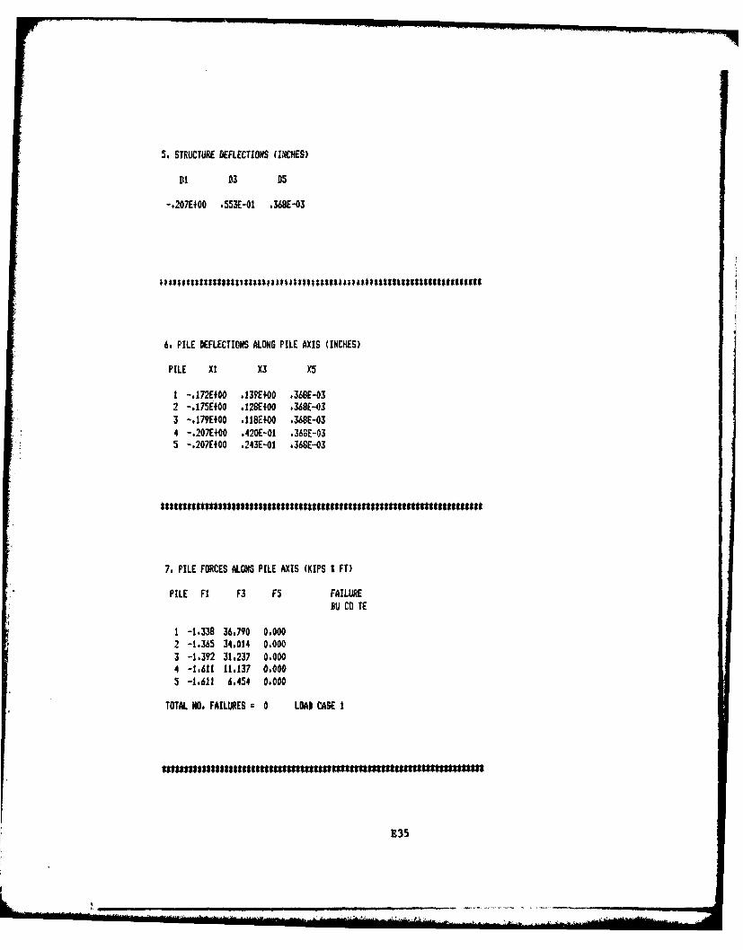
5. STRUCTURE DEFLECTIONS (INCHES)
Dl D3 05
-.207E+00 ,553E-01 .36BE-03
6. PILE DEFLECTIONS ALONG PILE AXIS (INCHES)
PILE Xl X3 X5
I -,172E+00 ,139E+00 -36BE-032 -.175E400 ,128E400 .36E-033 -.179E+00 .118E+00 .368E-034 -.207EI00 *420E-01 .368E-035 -.207E#00 .243E-01 .36E-03
7. PILE FORCES ALONG PILE AXIS (KIPS I FT)
PILE F1 F3 F5 FAILURERU CO TE
1 -1.338 36,790 0.0002 -1,365 34.014 0,0003 -1.392 31.237 0.0004 -1,611 11,137 0.0005 -1.611 6,454 0,000
TOTAL NO, FAILURES 0 LOAD CASE I
E35
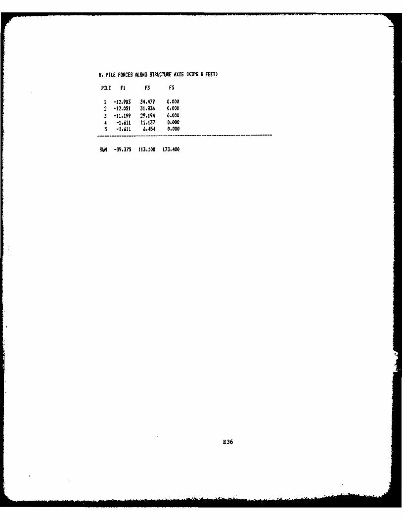
B. PILE FORCES ALONG STRUCTURE AXIS (KIPS a FEET)
PILE Fl F3 F5
1 -12,903 34.479 0.0002 -12.051 31,836 0.0003 -11.199 29.194 0.0004 -1.611 11,137 0,0005 -16611 6.454 0.000
--------------------------------------------
SUN -39,375 113.100 173.400
E36
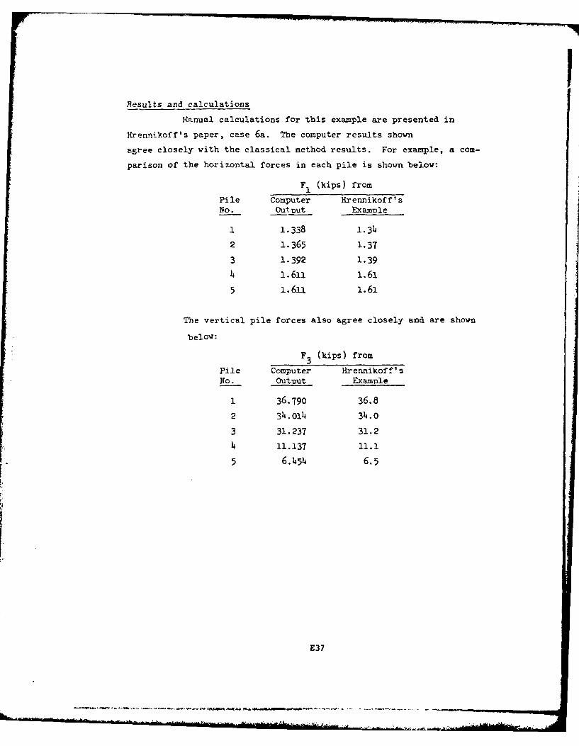
Results and calculations
Manual calculations for this example are presented in
Hrennikoff's paper, case 6a. The computer results shown
agree closely with the classical method results. For example, a com-
parison of the horizontal forces in each pile is shown below:
F1 (kips) from
Pile Computer Hrennikoff'sNo. Outp ut Exanle
1 1.338 1.334
2 1.365 1.37
3 1.392 1.39
14 1.611 1.615 1.61 1.61
The vertical pile forces also agree closely and are shown
below:
F (kips) from3Pile Computer Hrennikoff'sNo. Output Examnle
1 36,790 36.8
2 34.014 34.0
3 31.237 31.2
4 11.137 11.1
5 6.454 6.5
E37
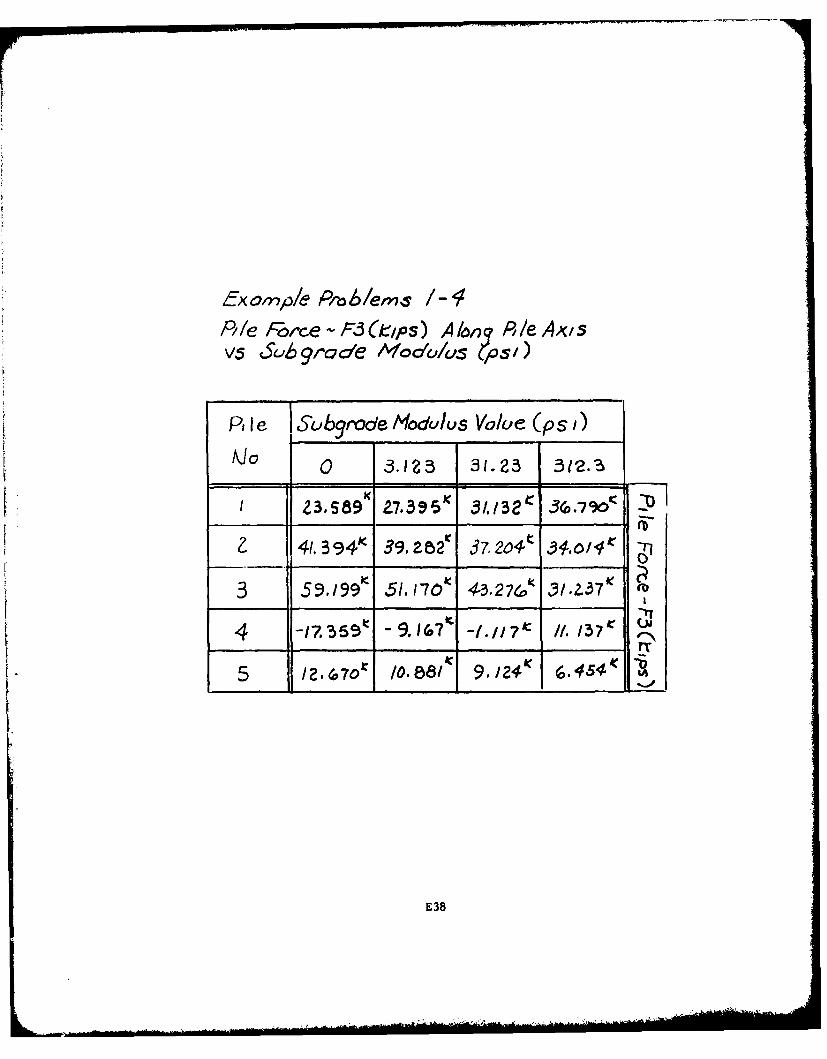
fxa mp/e Pno /,/erns I-Ple Force -F/:Ckps) A/aq P/e Axi sv5 Suh 9rode /f/oa'cu/(s i)
Pile 1Subrode/ModulusVolue (ps1)
Ado 0 3.112 a1.25 312.3
I Z3,S89 . 7 3T95 31/./3 3.-19o'
4t"39 4 9 9.ae,2 3742"43 93.5o'297 2o
3 59,199 51.170 43.276o 31.2-37
4 -17.55'c -9.1674 -//7t IH. /374rT
5 , /0.88 1 9./24 < 6.454
E38
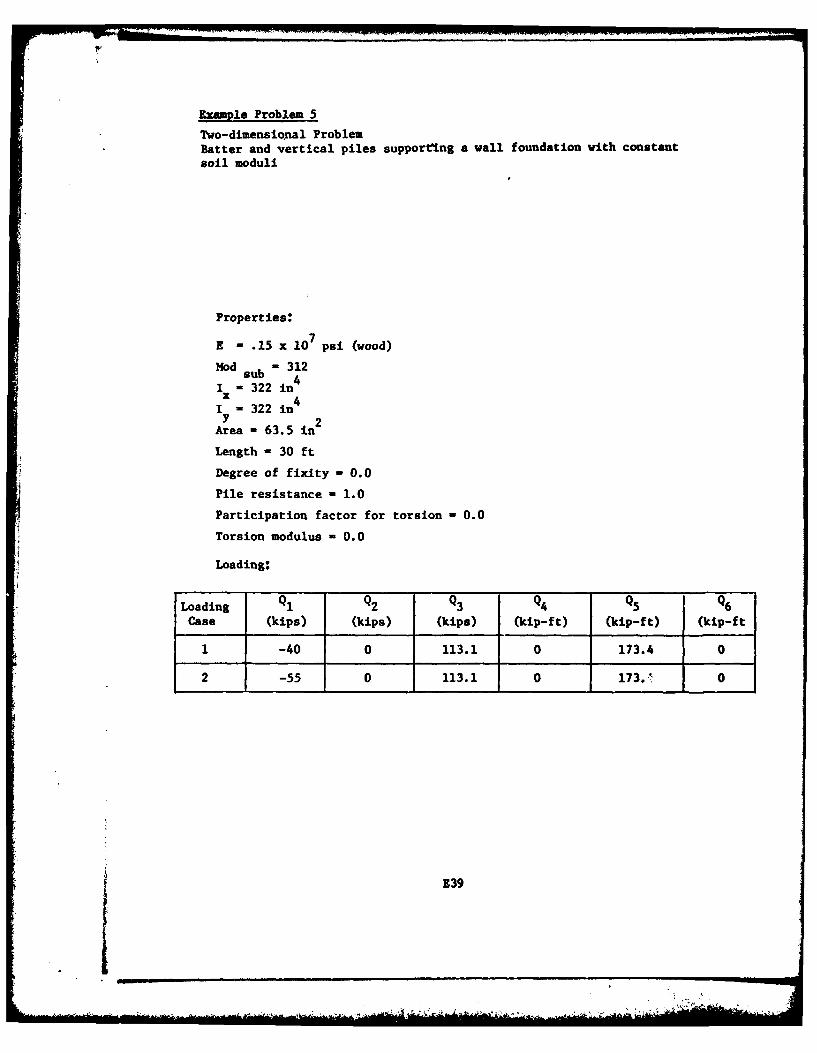
Example Problem 5
Two-dimensional ProblemBatter and vertical piles supportoing a vail foundation with constantsoil mnoduli
Properties:
E - .15 x 10 7psi (wood)
Mod -312
I - 2 in4
I = 322 in 4
y 2Area 63.5 in
Length - 30 ft
Degree of fixity - 0.0
Pile resistance -1.0
Participation factor for torsion -0.0
Torsion modulus -0.0
Loading:
Loading QlQ 2 Q3Q 4 QQ 6
Case (kips) (kips) (kips) (kip-ft) (kip-ft) (kip-ft_
1 -40 0 113.1 0 173.4 0
2 -55 0 113.1 0 173.,'. 0
f 139
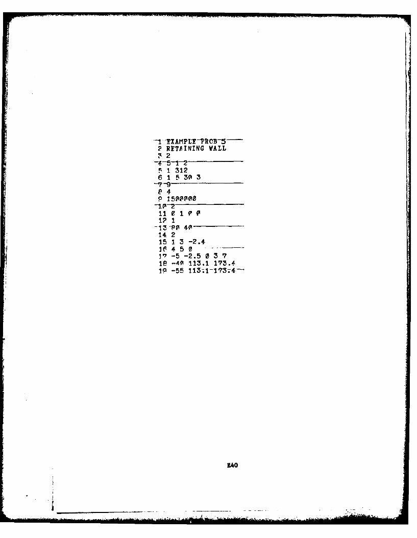
,- TXAMPL-PROB-5-2 RETAINING WALL
452
5 1 3126 1 530 3
--7-9-
E4p 1500000-1 c-211 0 1 CI? 1
-13-PVI 40- -
14 215 1 3 -2.4
V" -5 -2.5 03 7
19 -55 113;1-173;4-
240

T.IS PROGPAM GENERATES TE FOLLOWING TABLES:
TAM1E NO. CONTENTSI PILE AND SOIL DATA
--.--. -PILEILE-COORDINA TES-AN-BAAf RSTIFFNESS AND FLEXIBILITY MATRICES FOR THFSTRUCTURE AND COORDINATES CF ELASTIC CENTER
-- -4 - -APPLIED-LOADS5 STRUCTURE DEFLECTIONSf PILE DEFLECTICNS ALONG PILE AXIS
PI L-E-FORCES-A LONG-P-IL-E--*XI SPILE FORCES ALONG STRUCTURE 1XIS
INPUT THE NUMBERS OF THE TABLES FOR WHICE YOU WANT THE OUTPUT.SEPARATE TEE NUMBERS WITH COFMAS.
-I-N PUi--A-FI-!.-! NA,.M-FOR--'AB -E-8---!--'?,fiR*C f-E. -- tf5 LE3IF YCU WANT TO USE THIS INFCRMATION FOR A NEW RUNHIT A CARRIAGE RETURN IF YOU DO NOT WANT THIS FILE.
-I N 'UT-A--F HE-N AM E-FOR-OU TPUTI-N--C-AP-CTR--OR-L-ESS.EIT A CARRIAGE RETURN IF OUTPUT IS TO BE PRINTED CN TERMINAL.
EXAMPLE PROB 5--RETAINING-WA--.
-NO; -OF-P I LE-ROWS-------5 ]--tAT-I---It--OACLtULA TED OR -kt-f--
E41
* -- * -*I*
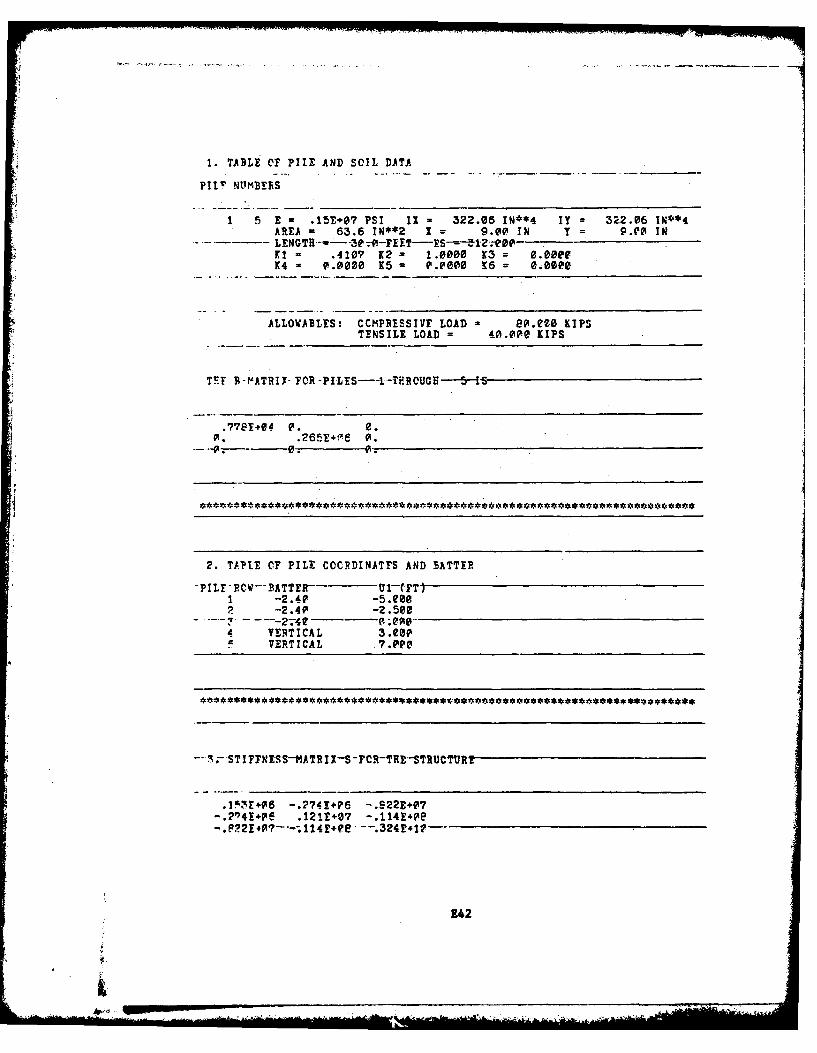
1. TABLE OF PIIE AND SOIL DATA
PIt" NUMBE.S
1 5 E = .15E+07 PSI IX = 322.06 IN**4 IT = 322.06 IN**4AREA = 63.6 IN**2 I = 9.@0 IN T = P.Po INLENGTE--- 30-;-F££T-ES--=--12.-eOP-KI = .4107 K2 = 1.0000 13 = 0.00K4 - 0.0000 K5 = P.0000 16 = 0.000
ALLOWABLES: CCMPRISSIVF LOAD e .es KiPSTENSILE LOAD = 40.000 KIPS
T B-fATRI FOR -PILES--I -THROUGH----"5-'5
.770e+04 P. 0.0. .265E+e 0.
2. TAME CF PILE COCRDINATFS AND BATTER
-PILF RCW- BATTER U I-(FT)1 -2.4? -5.e0o
-2.40 -2.500-.- -274? - - 0
4 VERTICAL 3.00VERTICAL .7.0PP
- ST I FES S"ATR I I-S-FCR-THE "STRUCTT R-
.1!E+06 -.274!+P6 -.622E+07-.2741+06 .121E+07 -.114E*Pe
-.P £ ¢-l-;11£+ --.324LP41--
E42
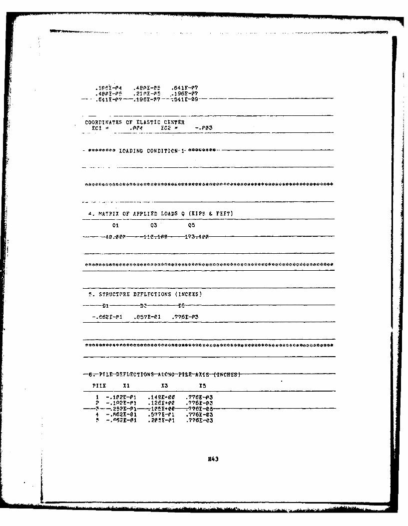
-- F 104 .4 LOPI~E-05 .54 1 F-09--
COORDINATES OF ELASTIC CE!NTEXECI M F02 = -.P03
- ~ LOADING
A. M~ATBIX OF APPLIED LOADS Q (KIPS &FEET)
01 Q3 Q5
5. STRUCTIURE DFFLFCTIONS (INCEES)
---- Di D:
-6 2rPLED-ECTI-ONSl CNO 77iE-A-!-(i4f3S
MIE xi X3 X5
1 -.102r-rX .l49E+e. .776E-03p -.102t-pI .12eF+02 .776r-Q'3
4 - .6621-01 .57?E-P'1 .776t-e~3
243
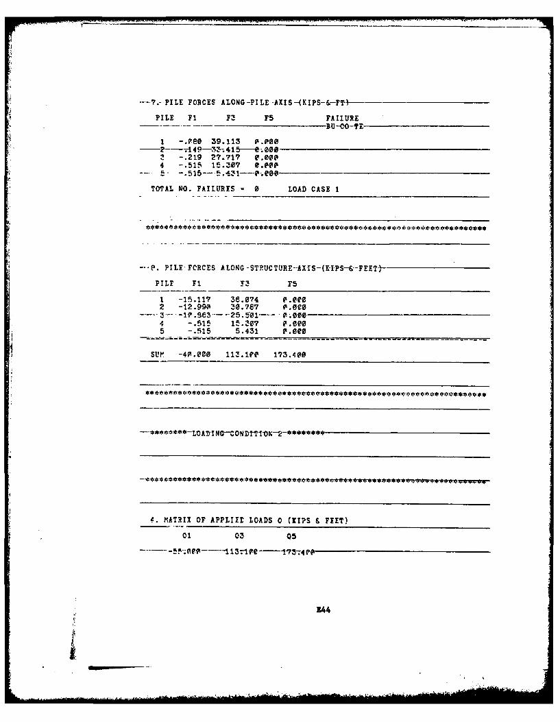
1
----7.-PILE FORCES ALONG-PILE AXIS-(KIPS---F--
PILE Fl F3 F5 FAIIURE
i -.Peo 39.113 .POO• -- --2 149--,3;415-----e000, -.219 27.717 0.0004 -.515 15.307 e.000
... 5- -5 5 -'. -- 0
TOTAL NO. FAILURES 0 LOAD CASE I
---P. PILE FORCES ALONG-STRUCTURE-'AXIS-(KI'PS-&-FEET-
PILE Fl F3 F5
1 -15.117 36.074 Vot2 -12.990 30.767 0.0e0
4 -.515 15.307 .e005 -.515 5.431 f.00
SUM -40.000 113.1?0 173.40e
4. MATRIX OF APPLIED LOADS 0 (NIPS & FEET)
01 03 Q5
944.. . ._____.. ..-"1_-""__ P

5. STRUCTURE DEFLECJONS (INCHES)
-f-;--?! L!-DELECT-I0NS- ALONG?I LE-f.X--S--HNC FES)
PILT X1 X.3 X5
I -1E .135E+00' - .185E-032 -. 325E+00 .14e.YQlQ -. lB5E-03
4 -. 345E40P .2C'!E-01 -. 185t-035 -. 345E+PP M29E-21 -. 1851-03
-- e*PIL1--FORCES-ALONG-P1!-E-AXIS--iK-rPS--&-rr)
PITT TI 73 F! FAILUREBU-CO--in-
1 -2.469 M6.770 0.00e
Z -2.43e 7e.487 O.M64 -2.e83 5.3Pe P.tceo
TOAt 'W0. FAI1URTS 0 LOAD CASE 2
E45
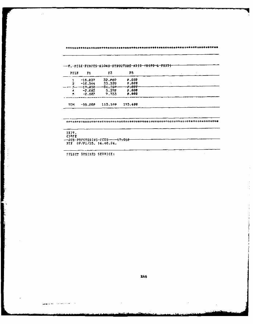
--e .---P I Lf-FORCES--A LON-STRUCTUR"I -- FS & F-iT-)
PILE Fl F3 F5
I -16.e37 32.Q'69 0.0ee2 -16.544 !3.329 2.000
A -2.E8" 5.37e 0.0005 -2.6V3 ?.733 91.000
SUM -55.OeP 113.10 173.400
XIT.C>,4y£
-JOB -PROCYSSI NG-C CUS-?- 910HE eP/01/25. 14.4e.24.
SFLECT DESIRED SERVICE:
E46

Computations
COMWN ANALYTICAL NETROD
.. CASE 1 4 0 k1 CASE R 5 5 'MU- 2081 in-kIin 3fl lengthof wall
1-H
ii, 34. -f
2.5' , 34~
LONGITUDINAL PILE SPACING
21 32
121. 011' 43- -
5. Az3C)4 -52V, 1,.02 V. 10 9V ,s
E47.
IA '2cI -i-II3.h~NNW-omnn2~

H 5 40.0j ~ 91.41 T- 38.0I 12 2.0k:I1000 lb/PILE OK
R5 zV5 V5
R4 V'V 4
5'V5
V 3 R2 : 3 4 k
VT 12 16 k R3 2 6 k
4 V2 CASE IR 4 - 16k
Ha 40.0
SCALE, 1" 100
-H 9.41 55.0
2 .11 .ri .5 k/PILE
R~x .6k V'SEXCEEDS 1.0 k/ PILE
R48 16, V4
*. V3
*1 ~CASE U 2 4
V 2 VTI2I.SR 3 - 26kV2 VTz 12.6 kR 4 * 16 k
VI R5 - 5.6k
'IV,
H. 55.0
SCALE' 1" 100
E48
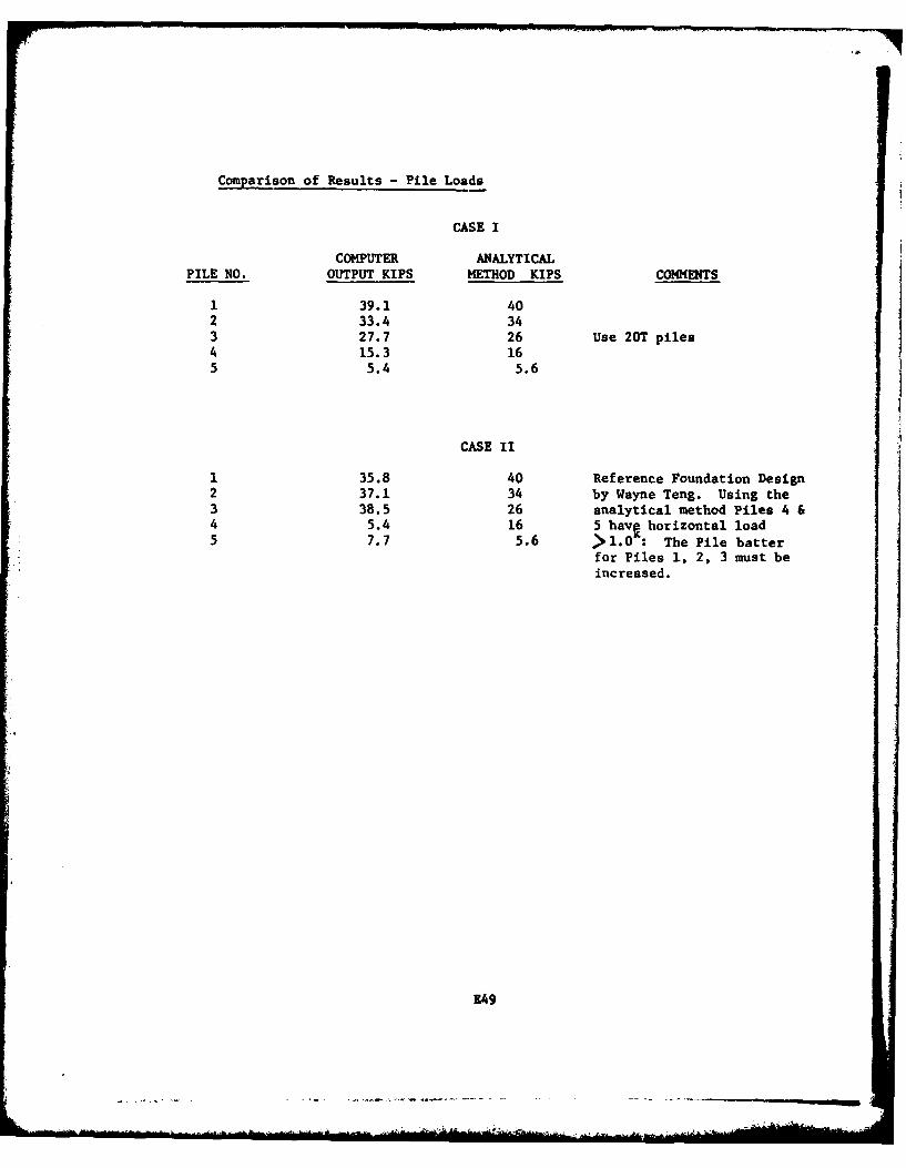
Comparison of Results - Pile Loads
CASE I
COMPUTER ANALYTICALPILE NO. OUTPUT KIPS METHOD KIPS COMMENTS
1 39.1 402 33.4 343 27.7 26 Use 20T piles4 15.3 165 5.4 5.6
CASE II
1 35.8 40 Reference Foundation Design2 37.1 34 by Wayne Teng. Using the3 38.5 26 analytical method Piles 4 &4 5.4 16 5 havn horizontal load5 7.7 5.6 >1.0-: The Pile batter
for Piles 1, 2, 3 must beincreased.
149
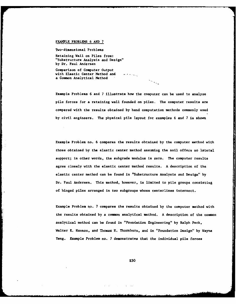
EXAMPLE PROBLEMS 6 AND 7
Two-dimensional Problems
Retaining Wall on Piles from:"Substructure Analysis and Design"by Dr. Paul Andersen
Comparison of Computer Outputwith Elastic Center Method anda Common Analytical Method
Example Problems 6 and 7 illustrate how the computer can be used to analyze
pile forces for a retaining wall founded on piles. The computer results are
compared with the results obtained by hand computation methods commonly used
by civil engineers. The physical pile layout for examples 6 and 7 is shown
Example Problem no. 6 compares the results obtained by the computer method with
those obtained by the elastic center method assuming the soil offers no lateral
support; in other words, the subgrade modulus is zero. The computer results
agree closely with the elastic center method results. A description of the
elastic center method can be found in "Substructure Analysis and Design" by
Dr. Paul Andersen. This method, however, is limited to pile groups consisting
of hinged piles arranged in two subgroups whose centerlines intersect.
Example Problem no. 7 compares the results obtained by the computer method with
the results obtained by a common analytical method. A description of the common
analytical method can be found in "Foundation Engineering" by Ralph Peck,
Walter E. Hanson, and Thomas H. Thornburn, and in "Foundation Design" by Wayne
Teng. Example Problem no. 7 demonstrates that the individual pile forces
ES0

Fefof/l/'q W// on P//esCom poi-vso, "w, ti /b &/oi c Cen /er /tie /,l0oJ
E 1. Cer. :::
Or n 2.4< --T/--77-- lFr 7TM 0
3.0 ,34 ;,II"I(,7 Z..
0
000
Figure E2. Physical problem for example problems 6 and 7
E51
obtained by this method are not alvays correct. For this particular problem,
the results do not compare favorably vith the results obtained by the computer
method. A subgrade modulus of 312 psi was used for the computer method.
E52

Example Problem 6
Two-dimensional problemretaining wall on pilesno lateral soil support
Properties
E -0.18 x 10 psi Degree of fixity = 0.0
Modsub = 10 psi 0 Pile resistance = 1.0
I - 1017.87 in.4 Participation factorx for torsion - 0.0
4I 1 1017.87 in. Torsion modulus - 0.0y
Area - 113.1 in.2
Length = 20.0 ft
Loading 1 3 5Case (kips) (kips) (kip-ft)
1 -60.0 192.0 -1218.0
Properties and loading conditionsfor example problem 6
E53
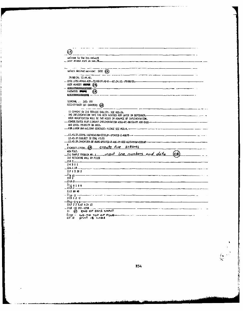
uelcoat to the bcs netw~ork....our. access p~rt.ds see...7
select desired service: EKSI
79/08124. 12.44.41.
USER NUMBER:
FASSWORD: M
TERMIINAL _ 205P flYkELIVER/USER In: CHAMREE.S
1O C04eENT CK Z?.S SERW'CE QUALITY, SEE 1155,26.* MS It(PLE11EHIAT:ON LATE HAS 9EEN REVISED' FOR LATER IN-SEPTEW~R, - _____________- -
USER NOT1VICATIGN UILL SE TVC LEEKS IN A~WKE OF W&LEmENTAIIOX.-CONSOLIATED PLOT-LIRAkY-4MPLEHENIAT104 -jL.44;6q FOR-EkSi
AND EKS2v 09/09/79 ON EKS3.-- FO.4R -LABOR -DAY-NOL IDAY -SCHEDULEt PLEASE -SEE-XSGY 4.
i-2.45.37.CP4SOTES/U-CECELt-aVpDATED-2-JG79....12.45,37.SUBJECT IS CERL FILES
_C)CEDI1,S!.4..R~it Creqte f'Ve ,Sr ROmLNEU FILE.
..J>1 SAMPLE MBOLEX-MO. I ,nigut line n rnhle,'S ?naf Wca4D2 RETAINING 94LL ON4 PILES
1>4 5 1 1
1)7 1 5 20 3
1>9 2
1>13 80 40
1)15 1 2 -2
1)17 2 2 5.67 9.34 13-1)18 -60 192 -12I8 . -. _________ - - - -- _________ - -D) ® two OF DATA -&Pu1r
D ?- cao --TO -top oir Ft e - - - - _ _- - _ _
E54
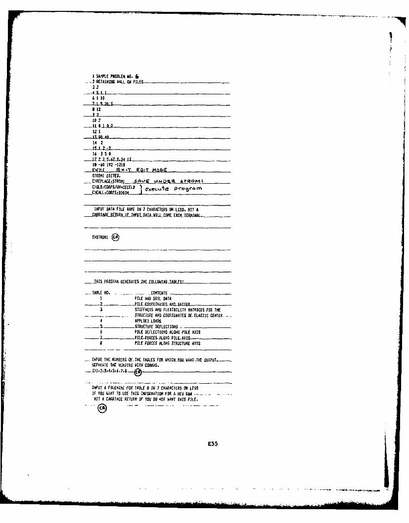
rI
II1 Sk4PLE PROBLEM NO. (s
-2 RETAINING WALL ON PILES--32
__-,.5LL
61107 1 R 2A A8 12
10 2_JL 1.O 012 111- 0-40
14 211 f 7 -2} , ,.s 15 0-16 350
1TZ 2.5,69L.34.13
18 -60 192 -1218_FIL F . tT Ef iT MOD _STROMI EDITED.C)REPLACEi5TROMJ 6A'g Li MOW ..TROM I
LD,CORPS/UNCECELl 3 eaecA prorra__CA.L ICORPSIO.34
INPUT DATA FILE HAVE IN 7 CHARACTERS OR LESS. HIT A_ CA-__RIAGU URX_I JULPDAmWILLCOM ER I.TERTAL.
I)STROMI
_..-THI SPO ,AM GENERATES -THE _EOLLOWING _TALES:
TALE NO, --CONTENTSI PILE AND SOIL DATA2. --- PILE.COCRDINATES- AND- BATTER3 STIFFNESS AND FLEXIDILITY MATRICES FOR THE
.. STRUCTURE AND COORDINATES OF- ELASTIC CENTER. - -4 APPLIED LOADS5 STRUCTURE DEFLECTIONS -6 PILE DEFLECTIONS ALONG PILE AXIS7 - RILEOCES- ALO,4-PILE-AXIfB PILE FORCES ALONG STRUCTURE AXIS
INPUT. THE IHMEERS OE' THE.TABLES FOR. WHICHYOU- I'ANT-THE OUIPUT.-SEPARATE THE NUMBERS WITH COMMAS,
-...-..... S...
INPUT A FILENAKE FCP TABLE 8 IN 7 CHARACTERS OR LESSIF YOU VANT TO USE THIS. INFORMATION FOR A NEW RUN --- - - - -HIT A CARRIAGE RETURN IF YOU DO CT WANT THIS FILE.
E55
------------------------- -- ---.-. - ~
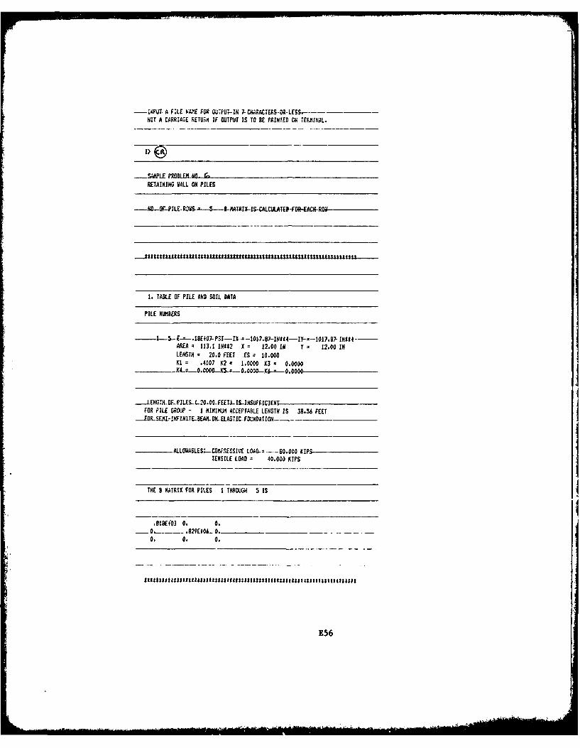
- 1PLUT A FILE ,ME FOR OUBFU.-I 7- CHA.ACTEAS-O2 LESS --MIT A CARRIAGE RETUI;A IF OUTPUT IS TO BE PRINTED ON TEEMINrL.
-SAMPLE PROBLE-NO r ,
RETAINING WALL ON PILES
-NO-OF-PLE-POS- ------ -MATRIY-IS-CALCLATE-FORAC.-ROj
.21UR**ttLOZ$Itt1I$1 .ZUUE IUtttl Iul***tILtUu*$$$tBUU tB.
1. TABLE OF PILE AND SOIL DATA
PILE NUMBERS
1 -5- - -.I8E 7-PS-IX =-07,87-I/tt4-Iy-=--O7,,67- INt$4--AREA z 113.1 INS92 X = 12.00 IN Y z 12.00 INLENGTH z 20.0 FEET ES = 10.000I = .4107 K2 1 1.0000 K3 z O.OOO0
K4-=- C0K5:O.Ooo-K6.---,O000
---.. LENGTHI OF_ ILES-.L 20 • DO- FEE II- IS-INSUEI CENTFOR PILE GROUP - I MINIMUM ACCEPTABLE LENGTH IS 38.56 FEETOR-SE 1 INFINLTE-BEA- ON. ELASIC.FDNDATIOn-
ALLOWASLESL-COMPRESSIVE LOAD-_. -0,000 KIPSTENSILE LOAD 40.000 KIPS
THE B MATRIX FOR PILES I THROUGH 5 IS
.IBEfO3 0. 0.O - _____. . 8 29E#06- 0 ... . .
0. 0. 0.
HtU**$ss2*10*50s2111$1100$*0zIaI$0000Ishua::u suahss$:usaE5S6IIfl
E56
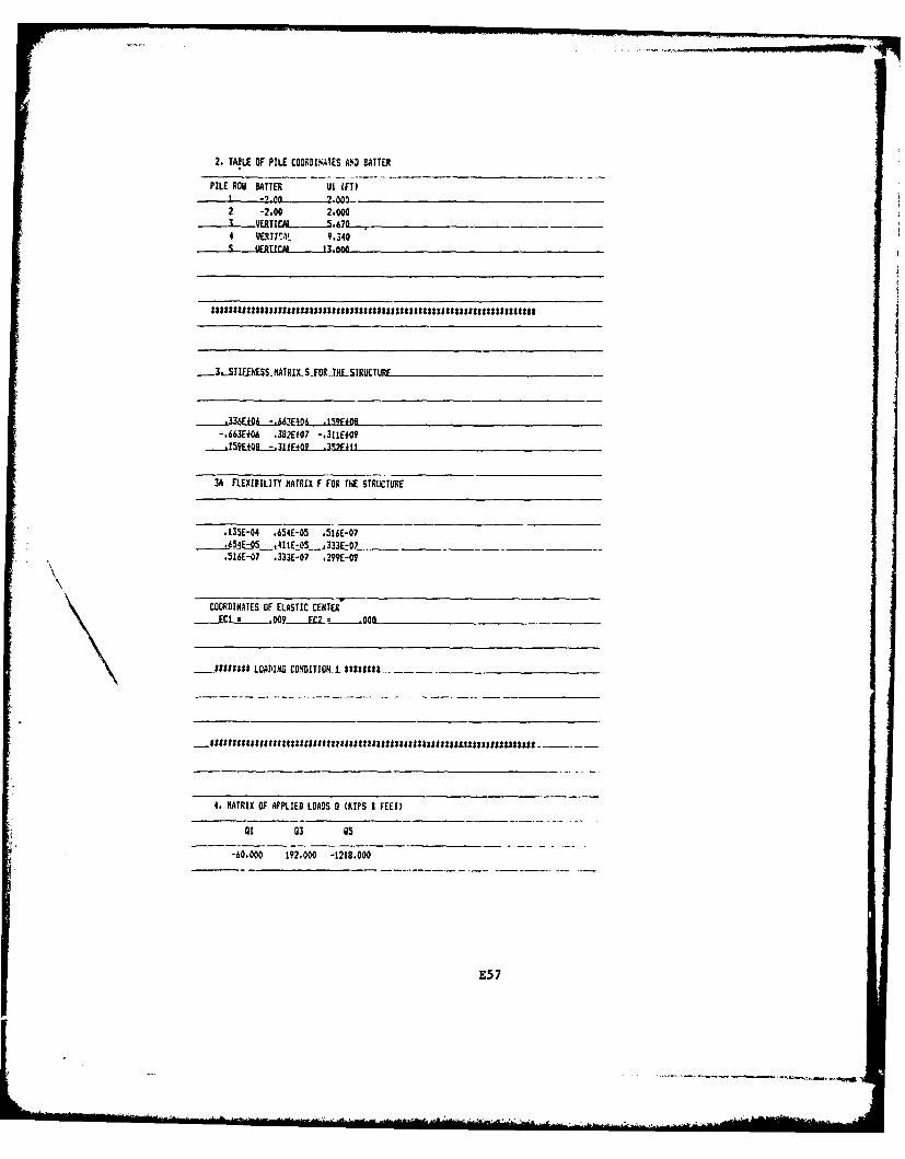
2. TABLE OF PILE COORDISATES A'-'D BATTER
PILE ROW BATTER Ul (FT)
2 -2.00 2.000I ERTICAL 5.67A
4 VERTICkl 9.340
-3..STIEEESS. MATRIX, S-ORTHESTRUCTURE
-. 66KE+06 .382E+07 -.311E409
3A FLEXIBILITY MATRIX F FOR THE STRUCTURE
.13SE-04 .6.14E-05 .516E-07
-516E-07 .333E-07 .2?9E-O?
COORDINATES OF ELASTIC CENTER
-1101403$$$ LOADING CONDITION, I 8081 ___________________
4. MATRIX OF APPLIED LOADS 0 (KIPS I FEET)
al 03 05
-60.000 192.000 -1218.000
E5 7
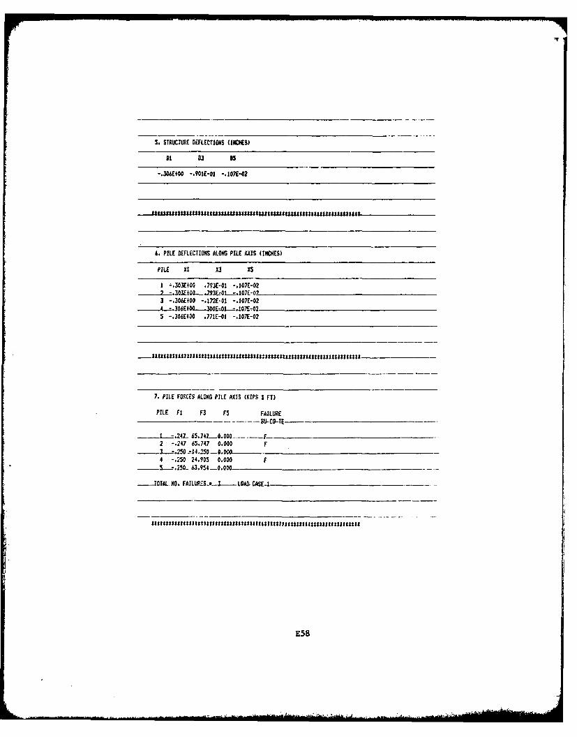
S. STRUCTURE DEFLECTIONS (INCHES)
o! 03 05
-. 306400 -. 901E-01 -. 107E-02
-..-. us ttuuu tUts u IuIugtagtuu $*sssssuuLaSsas$ s$ $ *us*$$*$*
6. PILE OEFLECTIONS ALONG PILE AXIS (INCHES)
PILE XI X3 X5
1 -,30KE+00 .773E-01 -.107E-02-.2.303E.O-..13 2-3 107-O?I -. 306E+00 -. 172E-01 -. 107E-024 .306Ef0-.-30OE 01--.. .I7E-025 -.306E400 .771E-01 -.107E-02
7. PILE FORCES ALONG PILE AXIS (KIPS I FT)
PILE FI F3 F5 FAILURE
- 1 -. 24L- 65.742---0.000-.---.F-
2 -.247 65.747 0.000 F.1 -. 250--.20-.64 -.250 24.905 0,000 F
-.250- 63.954.-0.000
. OTAL NO. FAILUPR:.'----.--LGALCASE-1
E58
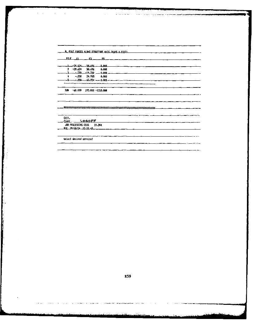
LEILEElRCESALDH&.-SICTURE.AXISw4JUFFl
P7 11 F1rgF
2 -29,624 58.696 0.000
4 -.250 24,705 0.000--K--. 250-- 63954 - 0.00- -________________
SLI -60.000 192.000 -1218.000
EXIT.-DY- LorsoFF
JOB1 PROCESSING CCUS 19.204..- Y-2910812".2.55.43
select d~esired service:
E59
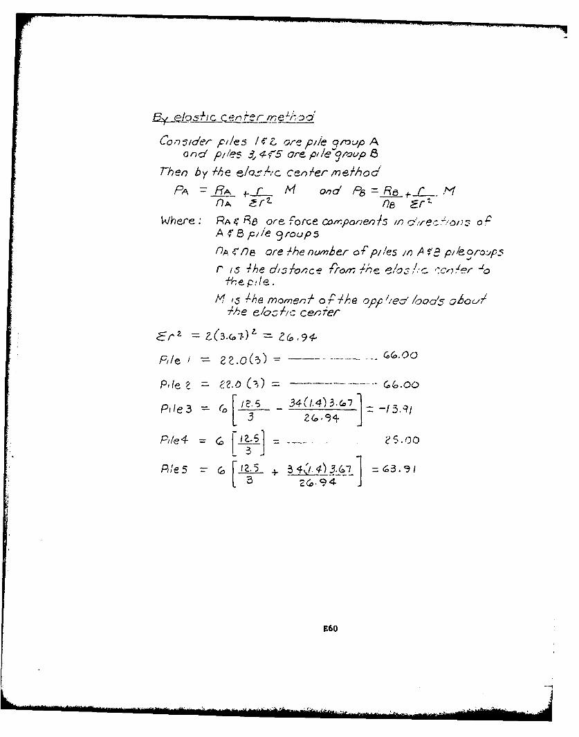
Coocrple5 s are pile qr~ic APr l ~/eS 5,4G- re pIle Oraup 8
r-heo by M~e e/oO:kc Ir~
PA = A M ,d P6 =e !aa
Where: RA ore force 0~Ypoe,. 4c ~r~:n ~A f 8 plle groups
fl~e~f~are 4he nwlnher 0 Pil/e5 ~A~pl r~p
r 1,5 4he d'srolc -in-_A t/5'.'~,!~
/ Ae m or e/-,74 o,r' IA e opp. e a c1 o,6 o u~-Me c /a0Ac c e',ef
pile / (-3 (14 3
2G.4
E60
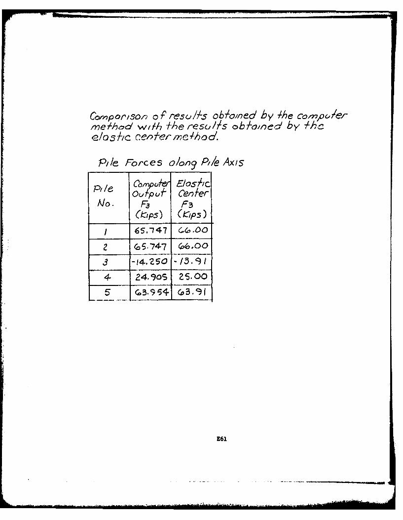
Coraportsor2 of7 Ileso/AS ob~olnec/ by Mhe Co r'1 pef-rnel-hoc wt//7 -Me reso/As obno/7c by -AC
Pile Forces o/on9 PA/e Axis
P/ile Compule E/057LlcOu/put ce/er
N~o. Fa3 F
/ ~5.74 7 (.~00
2 S5747 G6,0
4 24-190S 25.00
E61
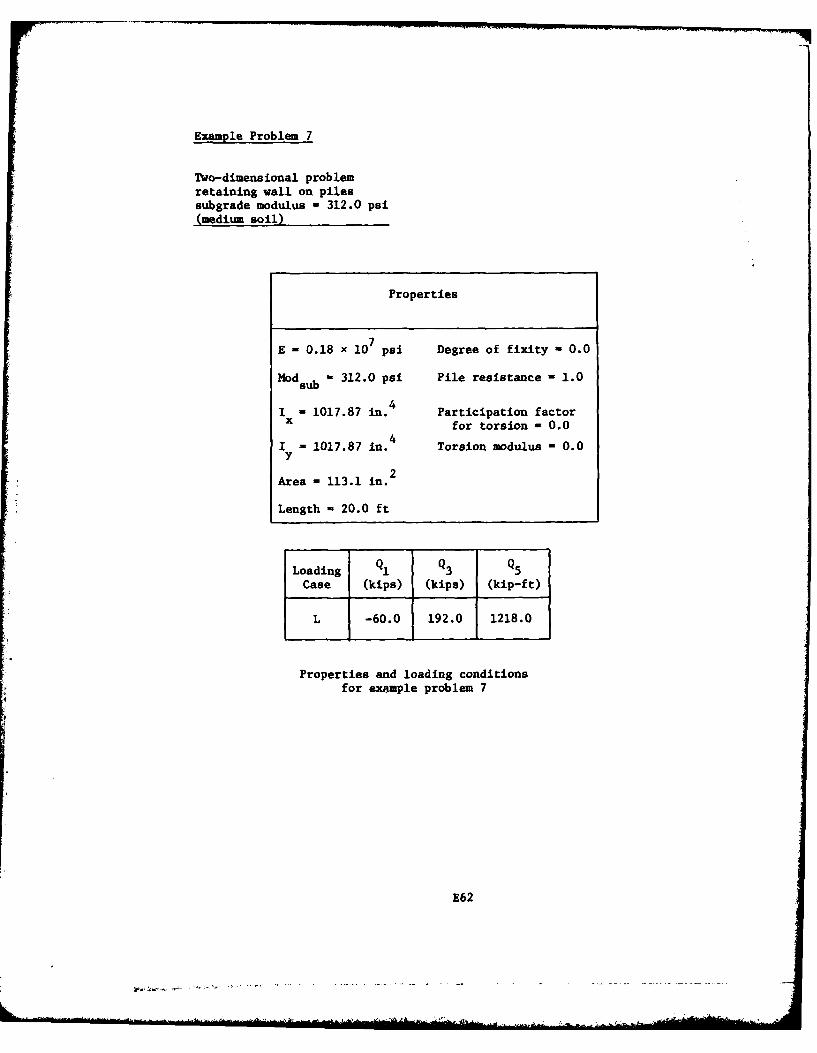
Example Problem 7
Two -dimensional problemretaining wall on pilessubgrade modulus - 312.0 psi(medium soil)
Properties
E - 0.18 x 10⁷ psi Degree of fixity 0.0
Modsu b ' 312.0 psi Pile resistance - 1.0
I - 1017.87 in.4 Participation factorx for torsion - 0.0
I - 1017.87 in.4 Torsion modulus - 0.0
2Area - 113.1 in.
Length - 20.0 ft
Loading Q1 Q3 Q5
Case (kips) (kips) (kip-ft)
L -60.0 192.0 1218.0
Properties and loading conditionsfor example problem 7
E62
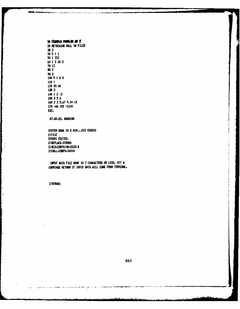
20 RETAINING MALL ON PILES30 240 5 1 150 1 312601 520 370 1280 290 2100 0 1 0 011o 1120 90 40130 2140 1 2-2150 3 5 0160 2 2 5,67 9,34 1317 G 0I 92-1117 -0 92-11
07.02,03, WARNING
SYSTEM ON IN 5 NIN.,.ECS ERRORSE)FILESTROMI EDITED,C>REPLACEPSTRONIC>WJCORPS/UlN:I1CELDC)CALLCRPSPX0034
INPUT DATA FILE NAME IN 7 CHARACTERS OR LESS. HIT ACARRIAGE RETURN IF INPUT DATA WILL COME FROM TERMINAL,
1)STROM1
E63
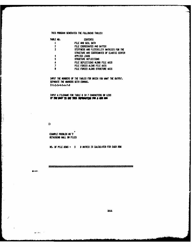
THIS PROGRAM GENERATES THE FOLLOVING TAKES:
TABLE NO. CONTENTSI PILE AND SOIL DATA2 PILE COORDINATES AND BATTER3 STIFFNESS AND FLEXIBILITY MATRICES FOR THE
STRUCTURE AND COORDINATES OF ELASTIC CENTER4 APPLIED LOADS5 STRUCTURE DEFLECTIONS6 PILE DEFLECTIONS ALONG PILE AXIS7 PILE FORCES ALONG PILE AXIS8 PILE FORCES ALONG STRUCTURE AXIS
INPUT THE NUMBRS OF THE TABLES FOR WIICH YOU MANT THE OUJTPUT,SEPARATE THE NUMEBERS 111TH COMMIAS.
12p3r4t5r6p7rB
INPUT A FILENAME FOR TABLE 8 IN 7 CHARACTERS OR LESS
I>
EXANPIE PROBLEM NO07RETAINING WALL ON PILES
NO. OF PILE RhlS r 5 1 MATRIX IS CALCULATED FOR EACH ROV
Z64
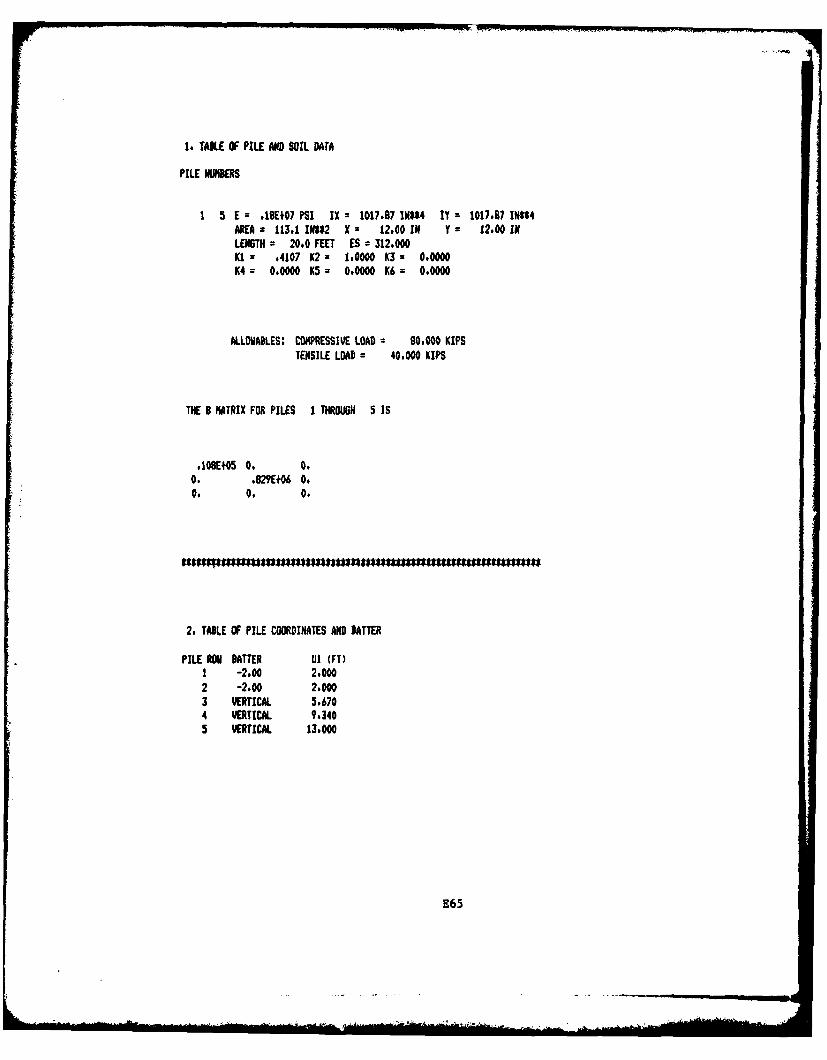
to TABLE OF PILE AND SOIL DATA
PILE NMBERS
1 5 E z .18E+07 PSI IX 1017.87 11(5* IY z 1017.87 11(5*4AREA z 113.1 INS*? X = 12.00 IN Y m 12.00 INLENGTH a 20.0 FEET ES = 312.000KI .4107 K2? 1.0000 K3 z 0.0000K4 = 0.0000 K5 0.0000 K6 = 0.0000
ALLOVABLES: COMPRESSIVE LOAD = 80.000 KIPSTENSILE LOAD = 40,000 KIPS
THE 3 MATRIX FOR PILES 1 THROUWH 51IS
l1OSEf05 0. 0.0. .929E+06 0.0. 0. 0.
2, TABLE OF PILE COORDINATES AND BATTER
PILE RON BATTER UI (FT)1 -2.00 2.0002 -2.00 2,0003 VERTICAL 5.6704 VERTICAL 9.3405 VERTICAL 13.000
E65
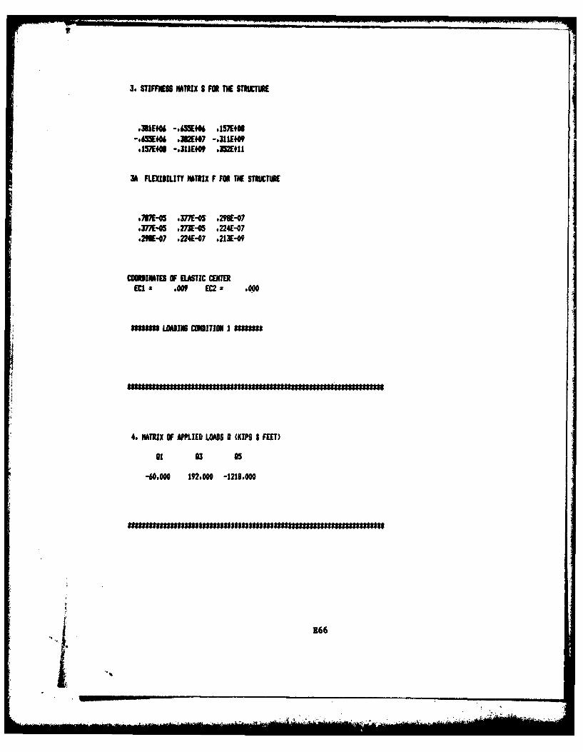
3. STIFFNESS MTRIX S FOR THE STUCTIME
.I311iO -. =5E06 .157E+06-*=.65E4 *3U2E47 -.311E09
#1570441 -.311E44 332E#II
3A FLEXISILITY MATRIX F FOR THE SThIETUlE
.737E-O5 .377E-O' #298E-07,377E-05 .273E-0 .224E-07,29-0 .224E-07 .213E-0
COORINTES OF ELASTIC CENTERECI s 0009 EC2 a 6000
888888 LOADING CONDITION I s8888*
4. MATRIX OF APPLIED LOADS I (KIPS I FEET)
01 03 05
-40.000 192.000 -1210.000
166
isA"

5, STRUCTURE DEFLECTIONS (INCHES)
Dl D3 D5
-. 1831400 o-.291-01 -,592E-03
6. PILE EFLECTIONS ALONG PILE AXIS (INCHES)
PILE Xl X3 X5
I -.171E+O0 .64E-01 -.592E-032 -.17lE+00 604E-Ol -.592E-033 -,l83E400 .IIOE-01 -. 5?2Z-034 -&183E+00 o370C-01 -. 592E-035 -"ll3E400 .6 30E0 - 592E-03
7. PILE FORCS AL.0 PILE AXIS (I(IPS F FT)
PILE Fl F3 FS FAILIUEBU CO TE
1 -1.842 56.762 0.0002 -1.842 56.762 0.003 -I.78 9.100 0.0004 -1.978 30.723 0.0005 -1.978 52.279 0.000
TOTAL NO. FAILURES a 0 LOAD CASE I
167
* I!
&
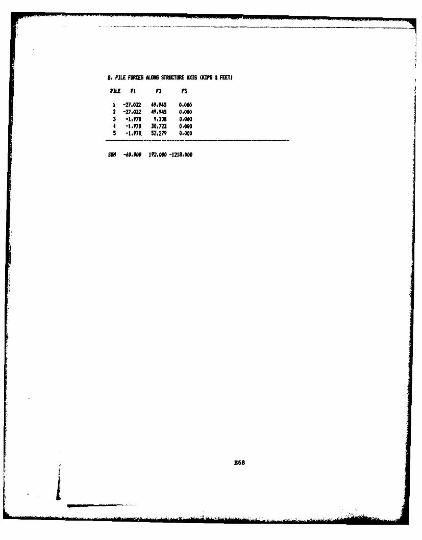
o. PILE FORCES ALONG STRucTURE Axis (KinS t FEET)
PILE Fl F3 FS
1 -27,032 49.945 0,0002 -27,032 49,945 0,0003 -1.978 9,108 0.0004 -1.978 30,723 0.0005 -1,978. 52,27N 0.000
SUN -60.000 192,000 -1218.000
E68

-0c e,:-;H/0 Kr
Po,rJ A * o-RestW/or,/-
C G of P1 /e,5 ordc cen 7r.,cc,
e= 69. CG - 8.(Co 0(o
Sz onol ecbor) 14/clul,>2.
(4 ?/.4- (.74)- 9 3)57 (6/eGO)
Pow 49/444 2.93= 'aipie P
Row. 5f 9A44 S-G IS.5 p//e-f
E69

8OwO3/~ /92 4 /s 5Z 3,4
5 /23.57
Row 5 1')? A /52 - -7. 5 7
C',
0')0le' 14
tC'
I.-n
Pile Flrce D1o3ronm Pile For~ce 0,ogrom,CarIFLpcier Ale/hoc! Common, Analvilco, M-e#/,oo
E70
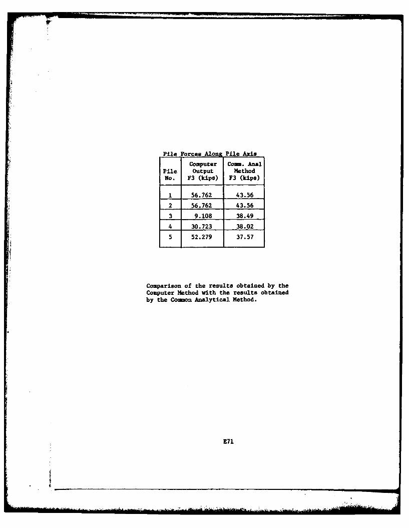
2U-
Pile Forces Along Pile Axis
Computer Comm. AnalPile Output MethodNo. F3 (kips) F3 (kips)
1 56.762 43.56
2 56.762 43.56
3 9.108 38.49
4 30.723 38.02
5 52.279 37.57
Comparison of the results obtained by theComputer Method with the results obtainedby the Comon Analytical Method.
171
' 1

EXAMPLE PROBLEMS 8 AND 9
3-dimensional ProblemsAschenbrenner' s ExampleComparison of Computer Outputwith Aschenbrenner's Calculations
Example problem 8 and 9 illustrate how the computer can be used to analyze
3-dimensional pile foundations problems. The following examples were taken
from Aschenbrenner's paper, entitled "Three-Dimensional Analysis of Pile
Foundations", published in the ASCE Journal of the Structural Division, Vol.
93, paper no. 5097, Feb. 1967, pp. 201-219. The computer results are compared
with Aschenbrenner's calcu ations. The physical pile layout for example problems
8 and 9 is shown in Figure E3.
Example Problem no. 8 compares the results of the computer method with Aschen-
brenner's calculations for a subgrade modulus of 35 pci, assuming the subgrade
modulus varies linearly with depth.
Example Problem no. 9 compares the results of the computer method with
Aschenbrenner's calculations for a subgrade modulus equal to zero; in other
words, assuming the soil offers no lateral support.
172

GO AI
Piles
LxUS 870 1/1~
I -. E a OO psi
£ 4
Figure E3. Physical problem for example problems 8 azkd 9
173
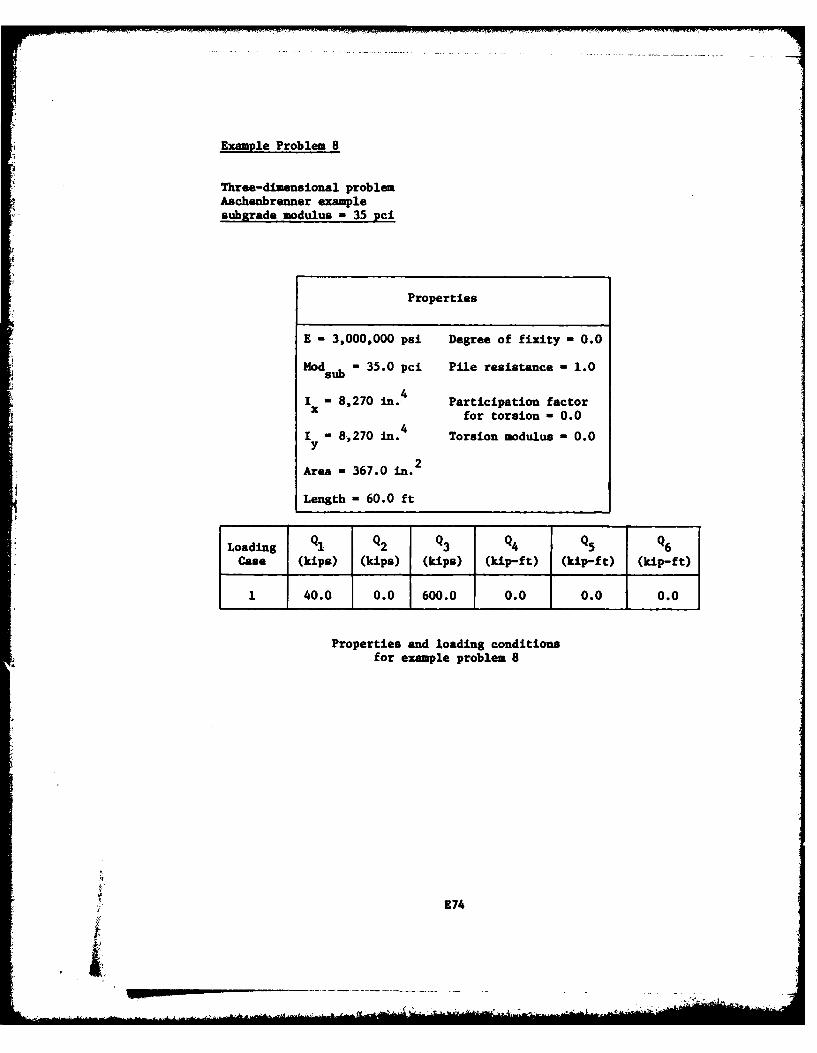
Example Problem 8
Three-dimensional problemAschenbrenner examplesubarade modulus -35 Pei
Properties
E 3,000,000 psi Degree of fixity -0.0
Mod sb- 35.0 pci Pile resistance -1.0
I x- 8,270 in. 4 Participation factorX for torsion - 0.0
I - 8.,270 in.4 Torsion modulus - 0.0y
Area - 367.0 in.2
Length - 60.0 ft
Loading Q' J J Q4 I 5 Q6Case (kips) (kips) (kips) (kip-ft) (kip-ft) (kip-ft)
14 0.0J0 .0 600.0j 0.01 0.0 0.0
Properties and loading conditionsfor example problem 8
174
.4 __

10 EXAMPLE PROBLEM NO Or ES:3S20 ASCI(NIRENNER CHECK30 340 9 1 1
0J 2 3560 1 9 60. 270 8270. 9270. 367. 16, 16,80 490 3000000,100 2110 04 it 0. 0.120 10, 10, 10. 150. 10, 10. 150. 10,130 0140 3, 45, 5. 5, 0.150 3. 90. 0. 5. 0.160 0, 0, 5. 0, 0.170 0, 0. 0. 0. 0.ISO 3. 135, -5. 5. 0.190 0. 0. -5. 01 0.200 3. 225, -5, -5, 0,210 3. 270, 0, -5. 0.220 3. 315, So -5, 0.230 40, 0. 600. 0, 0. 0,EWIoF>FILEqTROMh3 EDITFO.
r .REPLACEFSTRON3C>OLD9CORPS/UNzCECELJC>CALLPCORPSX0034
INVU DATA FILE NAME IN 7 CHARACTERS OR LESS. HIT ACARRIAGE RETURN IF INPUT DATA MILL COME FROM TERMINAL,
I>STROAJ
E75
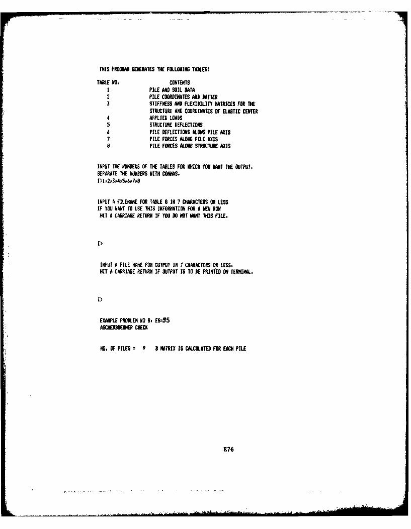
THIS PROGRAM GENERATES THE FOLLOWING TAKES:
TAKE NO. CONTENTSI PILE AND SOIL DATA2 PILE COORDINATES AND ATTER3 STIFFNESS AND FLEXIBILITY MATRICES FOR THE
STRUCTURE AND COORDINATES OF ELASTIC CENTER4 APPLIED LOADS5 STRUCTURE DEFLECTIONS6 PILE DEFLECTIONS ALONG PILE AXIS7 PILE FORCES ALONG PILE AXIS8 PILE FORCES ALONG STRUCTURE AXIS
INPUT THE NUMBERS OF THE TABLES FOR WHICH YOU WANT THE OUTPUT.SEPARATE THE NUMBERS WITH COMMAS.I1tI2t3t4p5,6v7p9
INPUT A FILENAME FOR TABLE 8 IN 7 CHARACTERS OR LESSIF YOU WANT TO USE THIS INFORMATION FOR A NEW RUNHIT A CARRIAGE RETURN IF YOU O0 NOT WANT THIS FILE,
I>
INPUT A FILE NAM4E FOR OUTPUT IN 7 CHARACTERS OR LESS.HIT A CARRIAGE RETURN IF OUTPUT IS TO BE PRINTED ON TERMINAL.
I>
EXAMPLE PROBLEM. NO 8, ES:35ASCHEHIBRENNER CHECK
NO. OF PILES z 9 B MATRIX IS CALCULATED FOR EACH PILE
E76
AA-i

1. TABLE OF PILE AND SOIL DATA
PILE NUMBERS
1 9 E a .30E+07 PSI IX :8270.0 INt4 IT:s 827.00 INSSAREA a 367.0 I10#2 X : 16.00 IN Y - 16.00 INLENGTH -- 60.0 FEET ES z 35.000K1 = .4107 K(2 1.0000 K(3 z 0.0000
K(4 z 0.0000 1(5 0.0000 1(6 z 4,0000
ALLO11ABLES: COMBINED BENDING FOR TENSION * 10.000 KIPSlWMf NT AWOT MINOR AXIS FOR TENSION x 10.000 KIP-FTMOMENT ABOUT MAJOR AXIS FOR TENSION z 10.000 KIP-FICOMBINED PENDING FOR COMPRESSION z 150,000 KIPSMOMENT ABOUT MINOR AXIS FOR COMPRESSION s 10.000 1(IP-FTMOMENT ABOUT MAJOR AXIS FOR COMPRESSION s 10.000 KIP-FTCOMPRESSIVE LOAD = 150.000 KIPSTENSILE LOAD z 10.000 KIPS
THE B MATRIX FOR PILES I THROUGH 9 IS
,499E+05 0. 0, 0. 0. 0.0. ,499E+05 0. 0. 0, 0,0. 0. *1511407 0. 0. 0.0. 0. 0. 0. 0. 0,
0. 0. 0. 0. 0. 0.
177

2. MilLE IF PILE COO1DIIMTES Am nTR
PILE NO, BATTER ANGLE UI(FT) U2(FT) U3(FT)1 3,00 45. 5,000 5.000 0.0002 3,00 90. 0.000 5.000 0.0003 ERTICAL 0, 5.000 0,000 0,0004 YERTICAl. 0. 0.000 0.000 0,0005 3,00 135, -5.000 5.000 0.0006 VERTICAL 0. -5.000 0.000 0,0007 3.00 225. -5.000 -5.000 0.0008 3.00 270. 0.000 -5.000 0.0009 3.00 315. 5.000 -5.000 0.000
3. STIFFNESS IIATRIX S FOR TIE STRUCTIRE
.745E+06 -,21Z-03 #769E-03 -. 922E-01 -#753E408 -. 894E-07-. 212E-03 .104E+07 O 4129E+09 -0540-01 -. 191E-01
.769E-03 0. .129E08 -. 477E-06 .477E-06 .146E100-. 922E-01 ,1291+09 -,477E-06 ,29KEll+ 0. -,43PE01-. 753E+O0 -. 540E-01 o477E-06 0. .309Ell .307E-04-o8?4E-07 -,191E-01 ,146#00 -#439E#01 *367F-04 ,215Ef10
3A FLEXIBILITY MATRIX F FOR THE STRUCTURE
.179E-05 -. 196E-15 -. 106E-15 .6M5E-17 .434E-0 -. 409E-23-.196E-15 .206E-05 -. 32BE-21 -. 88E-08 .312E-17 #164E-18-.106E-15 -. 32SE-21 .777E-07 ,265E-23 -,259E-18 -9527E-17
.635E-17 -.Ud6E-8 .265E-23 ,717E-10 -. 970E-26 ,675E-19
.434E-08 .312E-17 -. 259E-18 -.J79E-25 .430E-I0 -. 592-24-,409E-23 #104E-18 -. 527E-17 *675E-19 -. 599-24 #464E-09
88 888 LOADING CONDITIONI Jl8888
E78

4. MATRIX OF APPLIED LOADS 0 (KIPS I FEET)
a1 82 03 94 05 06
40.000 0.000 600.000 0.000 0.000 0.000
5. STh117!RE DEFLECTIONIS IICHEs)
Dl 2 13 94 35 D6
#71X1-01 -#704E-11 .466E-01 .254E-12 .174E-03 -.316E-11
PILE xi X2 X3 X4 XdX
I .364E-01 -,50E1-01 S50N-01 .117E-03 .123E-03 .389-042 -#147E-01 -#713E-01 .442E-01 .1651-03 -#316E-12 .5491-043 .7131-01 -#1991-09 .362E-01 .254E-12 .174E-03 -#316E-114 .713E-01 -.7841-11 .4691-01 .2W4-J2 .174E-03 -,316E-115 -.659E-01 -.504-01 .382E-01 .117E-03 -.1231-03 .39E-046 J711-01 .102E-09 .570E-01 .2541-12 .174E-03 -#3161-117 -.659E-01 .504E-01 .312-01 -.117E-01 -.123E-03 -.3891-048 -.147E-01 .7131-01 .442X-01 -.165E-03 .441E-12 -.5491-049 .364E-01 #504E-01 .5031-01 -,1171-03 *123E-03 -.389K-04
B79

7, PILE FORCES ALONG PILE AXIS (KIPS I FEET)
PILE F1 F2 F3 F4 F5 F6 CBFTR FAILURECl BU CO TE
1 1,814 -2.514 76.658 0,000 0,000 0,000 ,512 -. 735 -3,555 67.606 0:000 0.000 0.000 .453 3.555 -.000 55,321 0,000 0.000 0.000 .374 3.555 -.000 71,263 0.000 0.000 0,000 .485 -3,284 -2.514 59,354 0.000 0.000 0,000 .396 3,555 ,000 87,205 0,000 0.000 0,000 .597 -3,284 2,514 58,354 0,000 0,000 0,000 .398 -.735 3,555 67.606 0.000 0.000 0.000 .45
9 1.814 2.5f4 76.058 0,000 0,000 0,000 .51
TOTAL NO. FAILURES = 0 LOAD CASE 1
U*r***88****S***r**8*~~rlSSk~J1SS*S*$$***8*8*S8***SSSU$***$
8. PILE FORCES ALONG STRUCTURE AXIS (KIPS I FEET)
PILE Fl F2 F3 F4 F5 F6
1 20,190 16.625 72,340 0.000 0.000 0.0002 3.555 20,682 64.369 0.000 0,000 0.0003 3.555 -.000 55.321 0,000 0,000 0.0004 3.555 -.000 71.263 0.000 0.000 0,0005 -9.068 12,623 56.399 0.000 0.000 0,0006 3,555 .000 87,205 0,000 0.000 0.0007 -9,068 -12,623 56,398 0.000 0,000 0.0008 3.555 -20,682 64.369 0.000 0.000 0,0009 20,180 -16,625 72.340 0.000 0,000 0,000
SUM 40.000 -. 000 00.00 0,000 -.00 .000
E80

Pile Forces Along Pile Axis
Computer Aschen-Pile Output brennerNo. F3 (kips) F3 (kips)
1 76.858 79.7
I2 67.606 67.53 55.321 49.6
S4 71.263 71.3
I5 58.354 55.3
6 87.205 93.0
7 58.354 55.3
8 __67.606 67.5
r9-1 76.85879.7
Comparison of the results obtained by theComputer Method with the results obtainedby Aschenbrenner.
E81

Exiample Problem 9
Three-dimensional problemAschenbrenner exampleno lateral soil pressure
Properties
E =3,000,000 psi Degree of fixity =0.0
Mod, u .lpci A 0 Pile resistance =1.0
I a8,270 in. 4 Participation factorFX for torsion = 0.0
4I = 8,270 in. Torsion modulus - 0.0y
Area - 367.0 in.2
Length - 60.0 ft
Loading Q. Q2 3 Q4 Q5Case (kips) Ckips) (kips) (kip-ft) (kip-ft) _(kip-ft)
1 40.0 0.0 600.0 0.0 0.0 -J 0.0
Properties and loading conditionsfor example problem 9
E82

10 EXAMPLE PROBLEM NO 9p ES=020 ASCHENDPENNER CHECK30 340 9 1 150 2 .1to 1 9 60.?270 9270. 8270. 367. 16. 16.80 490 3000000.100 2110 0. 1. 0. 0.120 10. 10. 10. 150. 10. 10, 150. 10.130 0140 3. 45. 5. 5. 0.150 3. 90. 0. S. 0.160 0, 0. 5. 0. 0,170 0. 0. 0. 0. 0.180 3. 135. -5. 5. 0.190 0. 0. -5. 0. 0.200 3. 225. -5. -5. 0.210 3. 270. 0. -5, 0.220 3, 315, 5, -5. 0,230 40, 0. 600. 0. 0. 0,FoI.
C>REPLACEiSTRON3C4DLDCORPS/UN:CECELDC>CALLPCORPS.X0034
INPUT DATA FILE RANE IN 7 CHARACTERS OR LESS# HIT A
CARRIAGE RETURN IF INPUT DATA WILL CONE FROM TERMINAL.
I>STRDM3
E83
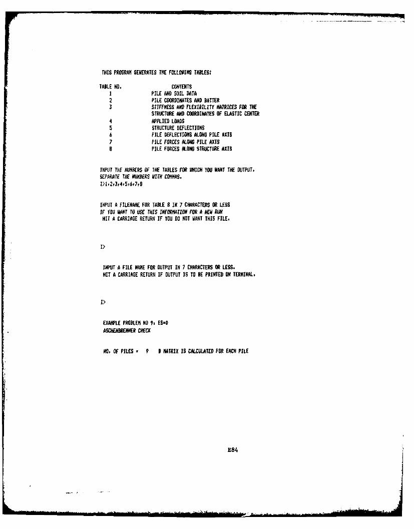
THIS PROGRAN GENERATES THE FOLLOZNG TABLES:
TABLE NO, CONTENTSI PILE AND SOIL DATA2 PILE COORDINATES AND BATTER3 STIFFNESS AND FLEXIBZLITY MATRICES FOR THE
STRUCTURE AND COORDINATES OF ELASTIC CENTER4 APPLIED LOADS5 STRUCTURE DEFLECTIONS6 FILE DEFLECTIONS ALONG PILE AXIS7 PILE FORCES ALONG PILE AXIS8 PILE FORCES ALONG STRUCTURE AXIS
INPUT THE NUMBERS OF THE TABLES FOR NHICH YOU VANT THE OUTPUT.SEPARATE THE NUMBERS VITH COMMAS.
INPUT A FILENAME FOR TABLE 8 IN 7 CHARACTERS OR LESSIF YOU WANT TO USE THIS INFORNATION FOR A HEU RUNHIT A CARRIAGE RETURN IF YOU DO NOT WANT THIS FILE.
I>
INPUT A FILE NAME FOR OUTPUT IN 7 CHARACTERS OR LESS.HIT A CARRIAGE RETURN IF OUTPUT IS TO BE PRINTED ON TERMINAL.
I>
EXAMPLE PROBLEM NO 9F ES=OASCHENBRENNER CHECK
NO. OF PILES 9 B MATRIX IS CALCULATED FOR EACH PILE
E84
iiL "" " , '
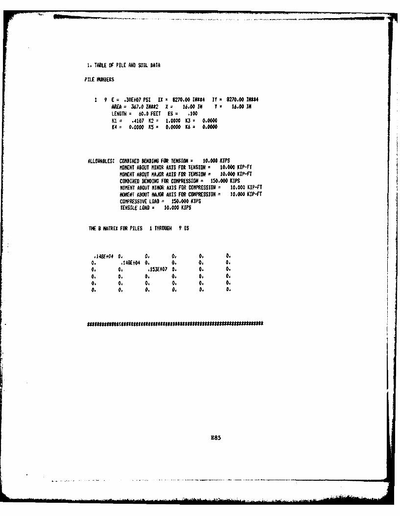
1. TABLE OF PILE AND SOIL DATA
PILE NUMBERS
1 9 E = .30E+07 PSI IX 9270,00 IN$*4 IY = 8270.00 IN$*4AREA = 367.0 JN*#2 X 16.00 IN Y a 16.00 INLENGTH = 60.0 FEET ES = .100KI1 .4107 K2 = 1.0000 K3 = 0.0000K4 = 0.0000 K5 = 0.0000 K6 = 0.0000
ALLONABLES: COMBINED BENDING FOR TENSION 10.000 KIPSMOMENT ABOUT MINOR AXIS FOR TENSION = 10.000 KIP-FTMOMENT ABOUT MAJOR AXIS FOR TENSION z 10,000 KIP-FTCOMBINED BEOING FOR COMPRESSION = 150,000 KIPSMOMENT ABOUT MINOR AXIS FOR COMPRESSION = 10.000 KIP-FTMOMENT ABOUT MAJOR AXIS FOR COMPRESSION = 10.000 KIP-FTCOMPRESSIVE LOAD = 150.000 KIPSTENSILE LOAD 10.000 KIPS
THE B MATRIX FOR PILES 1 THROUGH 9 IS
148E+04 9, 0, 0. O 0.0. .148E+04 0. 0, O. 0.0. 0. ,153E07 0. 0. 0.0, 0. O. 0. 0. 0.0. 0. 0. 0. O. 0,o O 0. 0. 0, 0.
E85
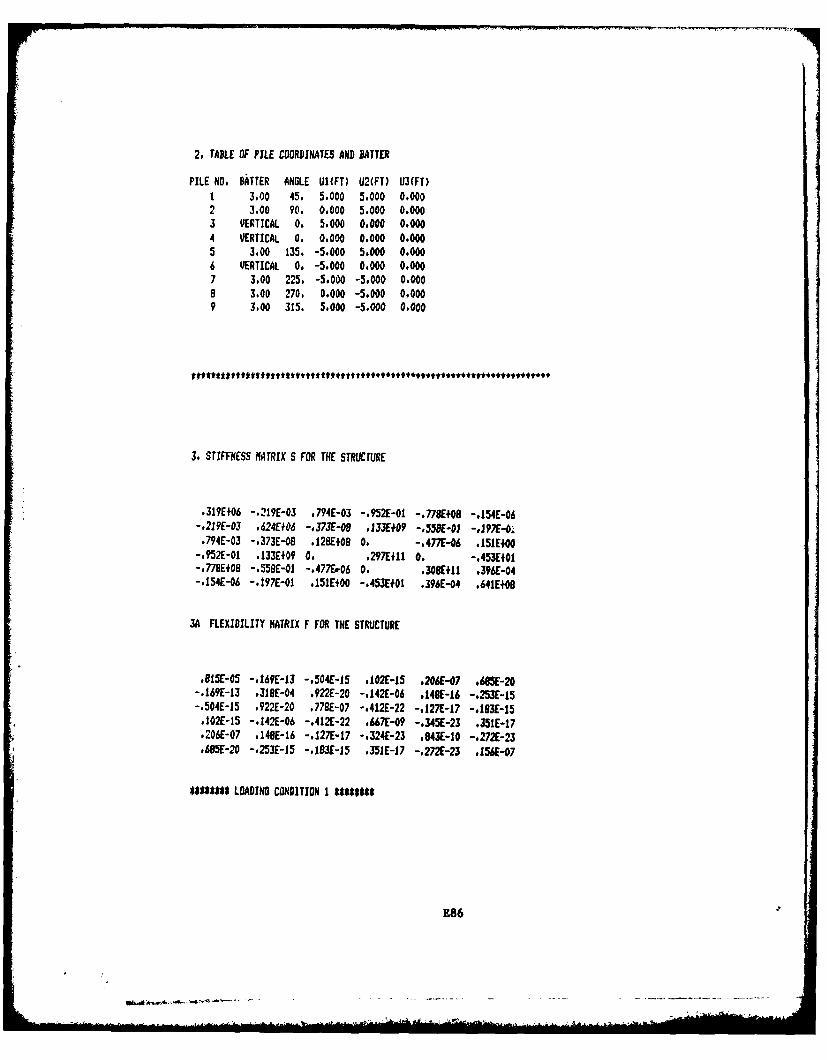
2. TABLE OF PILE COORDINATES AND PATTER
PILE NO, BATTER ANGLE UI(FT) U2(FT) U3(FT)1 3,00 45. 5.000 5,000 0,0002 3.00 90. 0.000 5.000 0.0003 VERTICAL 0. 5.000 0,000 0,0004 VERTICAL 0. 0.000 0.000 0.0005 3.00 135, -5.000 5.000 0.0006 VERTICAL 0. -5.000 0.000 0.0007 3.00 225. -5,000 -5,000 0.0008 3.00 270. 0,000 -5.000 0.0009 3.00 315. 5.000 -5.000 0,000
3. STIFFNESS MflTRIX S FOR THE STRUCTURE
.319E+06 -.219E-03 #794E-03 -,952E-01 -.778E+08 -,154E-06--219E-03 ,624E06 -#37E-O .133E#09 -.55SE-OJ -,JP7E-o..794E-03 -.373E-08 .128E08 0. -,477E-06 .151E+00
-,952E-01 ,133E+09 0. .297E411 0, -.453Et01-,778E408 -,55SE-01 -,477E.06 0. .30SE.11 .396E-04-.154E-06 -.197E-01 .151E.00 -.453E401 .396E-04 o641E+08
3A FLEXIBILITY MATRIX F FOR THE STRUCTURE
OISE-05 -.169E-13 -,504E-15 ,102-15 .206E-07 *68W-20-.169E-13 ,318E-04 .922E-20 -.142E-06 .148E-16 -.253E-15-.504E-15 .922E-20 .77SE-07 -,412E-22 -.127E-17 -,13E-15,IO2E-15 -.142E-06 -,412E-22 .667E-09 -.345E-23 .351E-17#206E-07 148E-16 -.127E-17 -.324E-23 .843-10 -.272E-23,685E-20 -.253E-15 -,13E-J5 .35JE-17 -.272E-23 #156E-07
$*Sttit LOADING CONDITION I $$lr$88$
E86
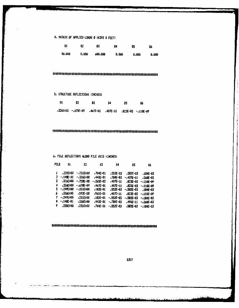
4. fATRIX OF APPLIED LOADS 9 (KIPS I FEET)
al 02 03 04 05 06
404000 0.000 600.000 0.000 0.000 0.000
5, STRUCTURE DEFLECTIONS (INCHES)
111 02 D3 D4 35 06
.326E+00 -,678E-09 ,467E-01 .407E-11 .823E-03 -.I1OE-O9
6. PILE DEFLECTIONS ALONG PILE AXIS (INCHES)
PILE X! X2 X3 X4 X5 X6
1 .220E+00 -. 23IE400 .704E-01 .552E-03 .582E-03 .IB4E-032 -. 14BE-0 -. 326E+00 .443E-01 .780E-03 -,437E-11 .260E-033 .326EI00 -.728E-08 -.26SE-02 .407E-11 .823E-03 -,llOE-0V4 ,326E400 -,67BE-09 .467E-01 .407E-11 .823E-03 -.11OE-095 -. 249E+00 -,231E+00 *182E-01 *552E-03 -. 582E-03 .184E-036 .326E*00 .593E-08 °961E-01 .407E-11 .823E-03 -.I1OE-097 -.249E#00 .231E+00 .182E-01 -.552E-03 -.582E-03 -.184E-03B -.148E-01 .326E+00 .443E-01 -.780E-03 .496E-11 -,260E-039 .220Ef00 .231E+00 .704E-01 -. 552E-03 .562E-03 -. 184E-03
E87
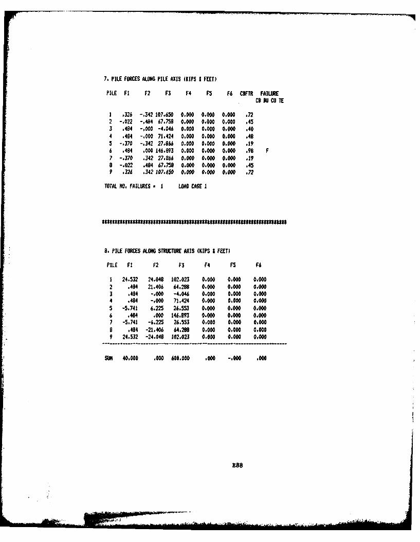
7. PILE FORCES ALONG PILE AXIS (KIPS I FEET)
PILE Fl F2 F3 F4 F3 F6 CBFTR FAILURE
CD DU CO TE
1 ,326 -.342 107.650 0,000 0.000 0,000 .722 -.022 -.484 67.758 0.000 0.000 0,000 .453 .484 -,000 -4.046 0.000 0.000 0.000 .404 .484 -.000 71.424 0.000 0.000 0.000 .485 -.370 -J342 27,866 0,000 0,000 0,000 .196 .484 .000 146.893 0.000 0,000 0.000 .98 F7 -,370 .342 27.866 0.000 0.000 0.000 ,198 -.022 .484 67.758 0,000 0,000 0,000 ,45P .326 .342 107,650 0,000 0,000 0.000 .72
TOTAL NO, FAILURES = 1 LOAD CASE I
9. PILE FORCES ALONG STRUCTURE AXIS (KIPS I FEET)
PILE Fl F2 F3 F4 F5 F6
1 24.532 24.048 102.023 0.000 0.000 0.0002 .484 21,406 64,288 0.000 0.000 0,0003 .484 -.000 -4.046 0.000 0.000 0.0004 .484 -,000 71,424 0.000 0.000 0,0005 -5.741 6.225 26,553 0.000 0,000 0,0006 .464 .000 146.993 0.000 0.000 0,0007 -5.741 -6,225 26.553 0.000 0,000 0,0009 .404 -21.406 64,288 0.000 0,000 0,0009 24.532 -24.048 102.023 0.000 0,000 0,000
SUN 40.000 .000 600.000 .000 -. 000 1000
E88
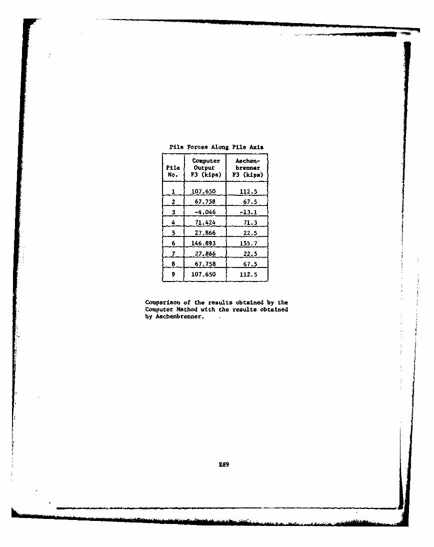
Pile Forces Along Pile Axis
Computer Aschen-Pile Output brennerNo. F3 (kips) F3 (kips)
1 107.650 112.5
2 67.758 67.5
3 -4.046 -13.1
4 71.424 71.3
5 27.866 22.5
6 146.893 155.7
7 27.866 22.5
8 67.758 67.5
9 107.650 112.5
Comparison of the results obtained by theComputer Method with the results obtainedby Aschenbrenner.
E89
-~
In accordance with letter from DM-MC. DAIN-ASI dated22 July 1977, Subject: Facsimile Catalog Cards forLaboratory Technical Publicatios, a facsimile catalogcard in Libray of Congress MIC format is reproducedbelov.
CAM Task Group on Pile Foundations.hse pile I oup behavior / by the CASE Task Oro on
Pile lmoudatios. Vicksbuwg, Mss. : U. S. Vaterwaysftperlmnt Static ; Springfield, Va. ; available frNational Technical Informtion Service, 1960.
22, [LI) p. : I. , 2T on. (Technical report -U. 8. Arm Enagineer Vpterwau hperlmmt Station ; K-80-5)
Prepated fr Office, COief of Egineers, U. S. Arm,Washington,. D. C.
References: p. 21-W.
1. omputer progres. 2. Coquterised simulation. 3. Delacriteria. 4. Pile foMdation design. 5. PAle foUndations.I. United States. Arm. Corps of Egineers. 17. Series:United States. Waterways Ixperlmt Station, Vickabug,Miss. Technical report ; X-80-5.
.AT.VA no.1-80-5
MEMO
4 .'.i-\4,4 A 3 PT
Stnaour EngiCmptrAts P lbk*uo In Report 0-70-2 Uspre Gufl. cowuut.Progrm Ah Intersve a
Grapico Wo Aosypfst*Plea frae tructur
Thnfli Begun K-1 Survy otfMfderinte Desig So","ar Mn low0
TeOMh Fksl S Ipru-0- Evaloion Of CoMPa PrograM for fth 4s*
-kPCA Or et Une'Gujdn towar prog.m-te#wmvj* f
$nfhjaton Rsp*" %4H A Tbrf0r*.na*$Nmeufhwtata :m l*ow
*niof q~dKS l 54Nramo*&WftA"O
krS~~~~eo~~~O& AemK4 A"al91iW SII i~s/w
4 4o t K 8 4O o u ~ t i t " f f " e w "
-7.