Embed Size (px)
Citation preview

283
Mechanical Pr7. Mechanical Properties
Materials used in engineering applications asstructural components are subject to loads, de-fined by the application purpose. The mechanicalproperties of materials characterize the responseof a material to loading.
The mechanical loading action on materialsin engineering applications may be static or dy-namic and can basically be categorized as tension,compression, bending, shear, and torsion. Inaddition, thermomechanical loading effects canoccur, (see Chap. 8 Thermal Properties). There mayalso be gas loads from the environment, leadingto gas/materials interactions (see Chap. 6 Surfaceand Interface Characterization) and to transportphenomena such as permeation and diffusion.
The mechanical loading action and the corre-sponding response of materials can be illustratedby the well-known stress–strain curve (for def-inition see Sect. 7.1.2). Its different regimes andcharacteristic data points characterize the me-chanical behavior of materials treated in thischapter in terms of elasticity (Sect. 7.1), plasticity(Sect. 7.2), hardness (Sect. 7.3), strength (Sect. 7.4),and fracture (Sect. 7.5). Methods for the determi-nation of permeation and diffusion are compiledin Sect. 7.6.
7.1 Elasticity .............................................. 2847.1.1 Development of Elasticity Theory .... 2847.1.2 Definition of Stress and Strain,
and Relationships Between Them .. 2857.1.3 Measurement of Elastic Constants
in Static Experiments .................... 2887.1.4 Dynamic Methods
of Determining Elastic Constants .... 2937.1.5 Instrumented Indentation
as a Method of DeterminingElastic Constants .......................... 296
7.2 Plasticity.............................................. 2997.2.1 Fundamentals of Plasticity ............ 2997.2.2 Mechanical Loading Modes Causing
Plastic Deformation ...................... 301
7.2.3 Standard Methodsof Measuring Plastic Properties ...... 302
7.2.4 Novel Test Developmentsfor Plasticity ................................ 310
7.3 Hardness ............................................. 3117.3.1 Conventional Hardness Test
Methods (Brinell, Rockwell, Vickersand Knoop) ................................. 313
7.3.2 Selecting a Conventional HardnessTest Method and Hardness Scale .... 319
7.3.3 Measurement Uncertainty inHardness Testing (HR, HBW, HV, HK) 321
7.3.4 Instrumented Indentation Test (IIT) 323
7.4 Strength .............................................. 3337.4.1 Quasistatic Loading ...................... 3337.4.2 Dynamic Loading ......................... 3427.4.3 Temperature
and Strain-Rate Effects ................. 3467.4.4 Strengthening Mechanisms
for Crystalline Materials ................ 3477.4.5 Environmental Effects ................... 3497.4.6 Interface Strength:
Adhesion Measurement Methods ... 350
7.5 Fracture Mechanics ............................... 3537.5.1 Fundamentals
of Fracture Mechanics ................... 3537.5.2 Fracture Toughness....................... 3557.5.3 Fatigue Crack Propagation Rate ...... 3637.5.4 Fractography ............................... 369
7.6 Permeation and Diffusion ..................... 3717.6.1 Gas Transport:
Steady-State Permeation .............. 3727.6.2 Kinetic Measurement .................... 3747.6.3 Experimental Measurement
of Permeability ............................ 3767.6.4 Gas Flux Measurement .................. 3787.6.5 Experimental Measurement
of Gas and Vapor Sorption ............. 3817.6.6 Method Evaluations...................... 3857.6.7 Future Projections ........................ 387
References .................................................. 387
PartC
7

284 Part C Measurement Methods for Materials Properties
7.1 Elasticity
Elastic properties of materials must be obtained by ex-periment methods. Materials are too complicated andtheories of solids insufficiently sophisticated to obtainaccurate theoretic determinations of elastic constants.Usually, simple static mechanical tests are used to eval-uate the elastic constants. Specimens are either pulledin tension, squeezed in compression, bent in flexure ortwisted in torsion and the strains measured by a varietyof techniques. The elastic constants are then calculatedfrom the elasticity equation relating stress to strain. Fromthese measurements, Young’s modulus, Poisson’s ratioand the shear modulus are determined. These are themoduli commonly used for the calculation of stressesor strains in structural applications. More accurate thanthe static method of determining the elastic constantsare the dynamic techniques that have been developedfor this purpose. In these techniques a bar is set intovibration and the resonant frequencies of the bar aremeasured. A solution of the elastic equations for the vi-bration of a bar yields a relationship between the elasticconstants, the resonant frequencies and the dimensionsof the bar. These techniques are about five times as ac-curate as the static techniques for determining the elasticconstants. Elastic constants can also be measured by de-termining the time of flight of an elastic wave througha plate of given thickness. Because there are two kindsof waves that can traverse the plate (longitudinal wavesand shear waves), the two elastic constants required forstructural calculations can be determined independently.Finally, the newest advances in techniques for measur-ing the elastic constants of materials have their originsin the need to measure these constants in thin films,or parts too small to be determined independently. Thedevelopment of nanoindentation devices proves to beideal for the measurement of elastic constants in thesekinds of materials. Each of these techniques is discussedin terms of standard American Society for Testing andMaterials (ASTM) and international test methods thatwere developed to assure repeatability and reliability oftesting. This discussion serves as a primer for engineersand scientists wanting to determine the elastic constantsof materials.
7.1.1 Development of Elasticity Theory
The design of new components for structural applica-tions usually includes an analysis of stress and strain toassure structural reliability. Two general kinds of prac-tical problems are encountered: the first in which all of
the forces on the surface of a body and the body forcesare known; the second in which the surface displace-ments on the body are prescribed and the body forcesare known [7.1]. In both cases, calculation of the stressesand displacements throughout the body and at the bodysurface is the objective. Within the limits of an elasticmaterial, i. e., a material in which the displacements andstresses completely disappear once all of the constraintsare removed, the theory for solving such problems wascompletely developed by the end of the 19th century.There are many methods of solving such problems, es-pecially with the development of finite element analysis.All such problems require the elastic constants of the ma-terial of interest as an input in order to obtain a solution.The description of experimental techniques of measur-ing the elastic constants of engineering materials are themain subject of this chapter, but before describing theexperimental techniques, we first give a brief history ofthe development of the theory of elasticity. We then goon to describe the theory of elasticity in order to put ourlater discussion of experimental techniques into con-text. There are several good books or chapters in booksthat give a history of the theory of elasticity [7.1–3],and there are many excellent texts that describe the the-ory [7.1,4]. The discussion given below rests heavily onreferences [7.1–4].
The first scientist to consider the strength of mater-ials was Galileo in 1638 with his investigation of thestrength of a rigid cantilever beam under its own weight,the beam being imbedded in a wall at one end [7.5]. Hetreated the beam as a rigid solid and tried to determinethe condition of failure for such a beam. The conceptsof stress and strain were not yet developed, nor was itknown that the neutral axis should be in the middle ofthe beam. The solution he obtained was not correct; nev-ertheless, his worked stimulated other scientists to workon the same problem.
The next important contributor to the theory of elas-ticity was Hooke in 1678, when he discovered the lawthat has been subsequently named after him [7.6]. Hefound that the extension of a wide variety of springs andspring-like materials was proportional to the forces ap-plied to the springs. This finding forms the basis of thetheory of elasticity, but Hooke did not apply the dis-covery to material problems. A few years later (1680),Mariotte announced the same law and used it to under-stand the deformation of the cantilever beam [7.7]. Heargued that the resistance of a beam to flexural forcesshould result from some of the filaments of the beam be-
PartC
7.1

Mechanical Properties 7.1 Elasticity 285
ing put into tension, the rest being put into compression.He assigned the neutral axis to one-half the height ofthe beam and used this assumption to correctly solve theforce distribution in the cantilever beam. Young furtherdeveloped Hooke’s law in 1807 by introducing the ideaof a modulus of elasticity [7.8,9]. Young’s modulus wasnot expressed simply as a proportionality constant be-tween tensile stress and tensile strain. Instead, he definedthe modulus as the relative diminution of the length ofa solid at the base of a long column of the solid. Never-theless, his contribution was used in the development ofgeneral equations of the theory of elasticity.
The first attempt to develop general equations ofelastic equilibrium was by Navier, whose model wasbased on central-force interactions between moleculesof a solid [7.10]. He developed a set of differen-tial equations that could be used to calculate internaldisplacements in an isotropic body. The form of theequations was correct, but because of an oversimplifica-tion of the force law, the equations contained only oneelastic constant.
Stimulated by the work of Navier, Cauchy in 1822developed a theory of elasticity that contained two elas-tic constants and is essentially the one we use todayfor isotropic solids (presented to the French Academyof Sciences on Sept. 30, 1822; Cauchy published thework in his Excercices de mathematique, 1827 and 1828.See footnote 32 in the first chapter of [7.3]). For non-isotropic solids, many more elastic constants are needed,and for a long time an argument raged over whetherthe number of constants for the most general type ofanisotropic material should be 15 or 21. The contro-versy was settled by experiments that were carried outon single crystals with pronounced anisotropy, whichshowed that 21 is the correct number of constants inthe most anisotropic elastic case. This number is alsosupported by crystal symmetry theory.
Once the theory of elasticity was completely devel-oped, equations could then be derived for experimentalmeasurement of the elastic constants. This has now beendone quite generally so that the techniques that have beendeveloped have a good scientific basis in the theory ofelasticity. Elastic constants can be measured statically(tension, compression, torsion or flexure), or dynami-cally through the study of vibrating bars, or by measuringthe velocity of sound through the material. Most of thesemeasurements are made on materials that are isotropic,so that only two constants are determined; however, withthe development of composite materials for structuralmembers, isotropy is lost and other constants have to beconsidered.
7.1.2 Definition of Stress and Strain,and Relationships Between Them
The theory of linear elasticity begins by defining stressand strain [7.1, 3, 4]. Stress gives the intensity of themechanical forces that pass through the body, whereasstrain gives the relative displacement of points within thebody. In the theory of linear elasticity, stress and strainare related by the elastic constants, which are materialproperties. In this section we define and discuss stressand strain and show how they are related through theelastic constants. It is these elastic constants that mustbe determined in order to evaluate stress distributions instructural components.
StressesWhen a body is under load by external forces, internalforces are set up between different parts of the body. Theintensities of these forces are usually described by theforce per unit area on the test surface through which theyact. One can imagine cutting a small test surface withina material and replacing the material on one side of thesurface by forces that would maintain the position of thesurface in exactly the same position as it was before thecut was made. As the size of the test surface is diminishedto zero, the sum of the forces on the surface divided bythe area of the surface is defined as the magnitude of thestress on the surface. The direction of the stress is givenby the direction of the force on the surface and need notbe normal to the surface.
From the definition of stress, it is clear that the stresson a surface will vary with orientation and position ofthe surface within the solid. It is also usual to breakdown the components of stress into stresses normal andparallel to the surface. The stresses parallel to the surfaceare called shear stresses. Because stress depends on boththe orientation of the surface, and the direction of theforces on the surface, the symbol indicating stress willhave two subscripts attached to it, the first indicating thesurface normal, the second indicating the direction of theforces on the surface. Consider a Cartesian coordinatesystem with three mutually perpendicular axes, x1, x2,and x3. A test surface normal to the x1-axis will havestresses, σ11, σ12, and σ13, where σ is the symbol forstress. The force indicated by the stress σ11 is on thex1-surface, and its orientation is parallel to the x1-axis.The stress σ11 is either a tensile stress (positive sign byconvention), or a compressive stress (negative sign). Thestresses, σ12 and σ13, are shear stresses: σ12 being on thex1-surface and oriented in the x2-direction; σ13 being onthe x1-surface and oriented in the x3-direction.
PartC
7.1

286 Part C Measurement Methods for Materials Properties
�
�
�
���
���
���
���
���
���
���
���
���
Fig. 7.1 Illustration of the two-index notation of stress.Stresses on the negative side of the cube have the oppo-site direction to those on the front side. Stresses in thefigure are all positive
An example of the stresses oriented around a smallcube is shown in Fig. 7.1. From the fact that the cubeis in equilibrium, the equation of equilibrium can bedetermined. Summing up the forces in the x1-direction,the following equation is obtained:
∂σ11
∂x1+ ∂σ12
∂x2+ ∂σ13
∂x3+ F1 = 0 , (7.1)
where F1 are the body forces in the x1-direction. Similarequations are found for the x2- and x3-axes.
A convenient shorthand representation has been de-veloped for equations similar to (7.1). The subscriptsof (7.1) are indicated by lower-case letters, usually i, j,and k. A partial derivative is indicated by a comma; a re-peated index indicates a summation. Thus, (7.1) can be
�
�
�
��
��
��
Fig. 7.2 On deformation, the size of the box has increased and theangles between the sides are no longer right angles, indicating botha tensile and a shear strain
represented by:
σij, j + Fi = 0 . (7.2)
Assignment of the value of 1, 2 and 3 for i yields threeindependent equations for equilibrium. The body forcesFi may be constant, or a function of space and time.
The state of equilibrium for the cube in Fig. 7.1 canalso be used to prove that σij = σ ji . Taking the mo-ment of the forces about a cube corner parallel to thex1-axis, σ23σ dx2(dx1 dx3) = σ32σ dx3(dx2 dx1), whichyields σ23 = σ32. Similar equations are obtained aroundthe x2- and x3-axis, proving the assertion that σij = σ ji .Therefore, of the nine possible stress components at anypoint within a body that is subjected to external forces,only six of them are independent.
StrainsStrains are determined by the relative displacements ofpoints within a body that has been subjected to externalforces. Imagine a volume within the body that was a cubeprior to deformation, but has now been deformed intoa general hexahedron, the axes of which may not be ofequal length, or the angles between them right angles(Fig. 7.2). Two types of strain can be defined from thisfigure: tensile strain, in which the length of the axes ofthe cube have been changed by deformation, and a shearstrain, in which the angle between the axes of the cubehave been changed by the deformation. If u representsthe displacement in the x1-direction of any point withinthe body due to the application of a set of forces, thenthe displacement of an adjacent point a distance dx1away from the first in a direction defined by the x1-axis is given by u + (∂u/∂x1)dx1. The relative changebetween the two points in the x1-direction is ∂u/∂x1,which is defined as the tensile strain in the x1-direction,ε11. Similar definitions are used for the tensile strainin the x2- and x3-directions: ε22 and ε33. In this case,v and w are the displacements in the y- and z-directions,respectively.
The shear strains are defined by the change in angleof the cube corners. Projecting the cube onto an x2–x3plane (Fig. 7.3), the change in the angle of the cubeis given by ∂v/∂x3 + ∂w/∂x2, where v and w are thedisplacements in the x2- and x3-direction, respectively.The strain ε23 is defined by ε23 = (∂v/∂x3 +∂w/∂x2)/2.Similar equations are obtained for ε12 and ε13. As withthe shear components of the stress tensor εij = ε ji , ascan be seen from the definition of shear strain.
Some other properties of stress and strain are com-mented on without proof. Both stress and strain aretensor quantities and transform as tensors with the rota-
PartC
7.1
Mechanical Properties 7.1 Elasticity 287
tion of system axes. Consider a transformation of axesfrom xi , x j , xk to xα, xβ , xγ , then the stresses willtransform according to the following equation:
σαβ = lαi lβ jσij , (7.3)
where lαi and lβ j are the cosines of the angles betweenxα and xi , and xβ and x j , respectively. Once the σijare obtained at a point for a given set of axes, they canbe obtained for any other set of axes using this simpletransformation.
Stress–Strain RelationsFinally we arrive at the set of equations that relate stressand strain. Since there are six independent componentsto the stress tensor and six independent components tothe strain tensor, there will be 36 constants of propor-tionality connecting the two
σij = Cijklεkl . (7.4)
The coefficients Cijkl are the elastic stiffness constants.The repeat of the index kl in the subscripts on theright-hand side of this equation indicate by conventiona summation over these subscripts for k = 1, 2 and 3 andsimilarly for l. Thus, for each of the six stress compo-nents on the left-hand side of the equation, there are sixterms on the right-hand side and six coefficients Cijkl .Of the 36 constants, it can be shown by strain-energyconsiderations that only 21 are independent. This num-ber is reduced further by the symmetry of the solid. Fora cubic material, the number of elastic constants is re-duced from 21 to three. For an isotropic material, the
���
���
��
��
�
�
���������
���������
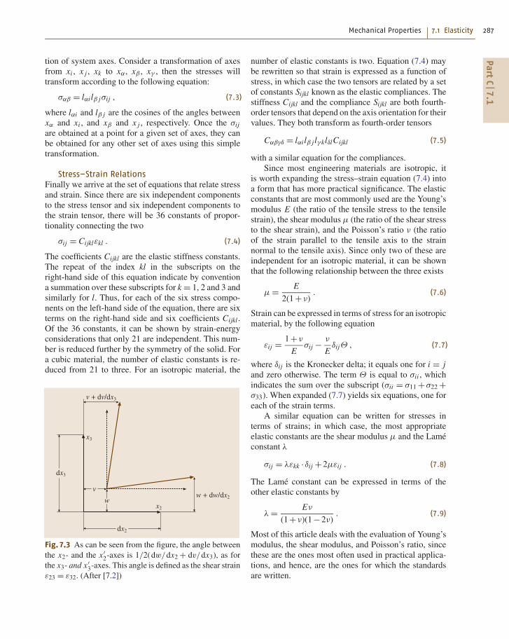
Fig. 7.3 As can be seen from the figure, the angle betweenthe x2- and the x′
2-axes is 1/2(dw/dx2 + dv/dx3), as forthe x3- and x′
3-axes. This angle is defined as the shear strainε23 = ε32. (After [7.2])
number of elastic constants is two. Equation (7.4) maybe rewritten so that strain is expressed as a function ofstress, in which case the two tensors are related by a setof constants Sijkl known as the elastic compliances. Thestiffness Cijkl and the compliance Sijkl are both fourth-order tensors that depend on the axis orientation for theirvalues. They both transform as fourth-order tensors
Cαβγδ = lαi lβ j lγklδlCijkl (7.5)
with a similar equation for the compliances.Since most engineering materials are isotropic, it
is worth expanding the stress–strain equation (7.4) intoa form that has more practical significance. The elasticconstants that are most commonly used are the Young’smodulus E (the ratio of the tensile stress to the tensilestrain), the shear modulus μ (the ratio of the shear stressto the shear strain), and the Poisson’s ratio ν (the ratioof the strain parallel to the tensile axis to the strainnormal to the tensile axis). Since only two of these areindependent for an isotropic material, it can be shownthat the following relationship between the three exists
μ = E
2(1+ν). (7.6)
Strain can be expressed in terms of stress for an isotropicmaterial, by the following equation
εij = 1+ν
Eσij − ν
EδijΘ , (7.7)
where δij is the Kronecker delta; it equals one for i = jand zero otherwise. The term Θ is equal to σii , whichindicates the sum over the subscript (σii = σ11 +σ22 +σ33). When expanded (7.7) yields six equations, one foreach of the strain terms.
A similar equation can be written for stresses interms of strains; in which case, the most appropriateelastic constants are the shear modulus μ and the Lameconstant λ
σij = λεkk · δij +2μεij . (7.8)
The Lame constant can be expressed in terms of theother elastic constants by
λ = Eν
(1+ν)(1−2ν). (7.9)
Most of this article deals with the evaluation of Young’smodulus, the shear modulus, and Poisson’s ratio, sincethese are the ones most often used in practical applica-tions, and hence, are the ones for which the standardsare written.
PartC
7.1

288 Part C Measurement Methods for Materials Properties
Linear elastic solutions of boundary problems canbe obtained using the relationships between stress andstrain (7.7) or its inverse (7.8) and the equations of equi-librium (7.2) subject to the conditions at the boundary.The solutions must satisfy a set of six equations known asthe compatibility relations. These equations assure thatsolutions obtained yield valid displacement fields, i.e.fields in which the body contains no voids or overlappingregions after deformation.
The experimental configurations normally used todetermine the elastic constants are cylinders of circu-lar or rectangular cross sections, which are loaded intension, flexure or torsion. Under static loading, elasticmoduli are calculated from the load on the specimen,a measurement of specimen displacement and an elasticsolution for the particular specimen. Measurements canalso be made by dynamic techniques that involve reso-nance, or the time of flight of an elastic pulse through thematerial. In general, the static technique yielded resultsthat are not as accurate as those obtained dynamically,differing by about −5% to +7% of the mean value of thedynamic technique [7.11]. The difference may be due toa combination of effects (adiabatic versus isotropic con-ditions, dislocation bowing, other sources of inelasticity,and different levels of accuracy and precision). This isdiscussed in Sect. 7.1.4.
In the remainder of this chapter, the techniques fordetermining the elastic constants for isotropic materialsare discussed. The most recent ASTM recommendedtests will form the basis of the discussion. The standardsthat are currently in use will be described and their ap-plication to a given material will be discussed. Sincematerials have a wide range of values for their elas-tic properties, given standards are not suitable for allmaterials. So, in the course of the discussion, the stan-dards will be discussed with reference to the differentclasses of materials (polymers, ceramics, and metals)and recommendations will be made as to which tech-nique is preferred for a given material. The relative errorof each standard measurement will also be discussedwith reference to the various materials.
Although ASTM tests are used in our discussions,we recognize that these standards are not universal.Other countries use different sets of standards. Never-theless, the standards for elastic constants are all basedon the same set of elastic equations and the same physi-cal principals. So, regardless of which standard is used,the investigator should obtain identical results withinexperimental scatter. Furthermore, the same materialconsiderations have to be taken into account in estab-lishing a standard measurement technique. So here too,
the standard tests will have to be similar to obtain a givenaccuracy. A list of European standards is given in theappendix for those readers who prefer to use standardsother than ASTM.
Five general tests are used to determine the elasticconstants of materials. Tensile testing employing a staticload is used to measure Young’s modulus, and Poisson’sratio. Torsion testing of tubes or rods is used to deter-mine the shear modulus. Flexural testing under a staticload is used to determine Young’s modulus. Various ge-ometries are used for the flexural tests. Finally, resonantvibration of long thin plates and the time of flight ofsonic pulses are both used to measure Young’s modulusand the shear modulus.
7.1.3 Measurement of Elastic Constantsin Static Experiments
In principal the simplest test geometry for determin-ing elastic constants is the tensile test. A fixed load isplaced on the ends of the specimen and the displace-ment over a fixed portion of gage section is measured.The load divided by the cross-sectional area gives thestress and the displacement divided by the length overwhich displacement was measured gives the strain. TheYoung’s modulus is then given by the stress divided bythe strain. Often, the Young’s modulus is measured aspart of a test carried out to determine the plastic prop-erties of the metal. In such a test, a stress–strain curveis obtained on the metal, and the linear portion of thecurve at the beginning of the test is used to calculate theYoung’s modulus. At the same time, if the lateral dimen-sions of the specimen are measured during the test, thetest results can be used to determine Poisson’s ratio asa function of strain.
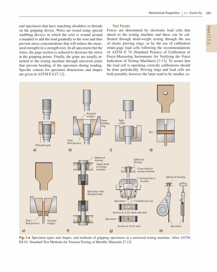
Test SpecimensTensile tests are generally carried out on a universaltest machine. The precautions needed to achieve highmeasurement accuracy include alignment of the test ma-chine, calibration of the load cell, firm attachment ofthe extensometers used to measure strain, and accuratemeasurement of the dimensions of the specimen crosssection. Examples of specimen types and shapes, andmethods of gripping used in these machines are shownin Fig. 7.4 [7.12]. The type of specimen depends on thestock from which the specimen is taken. Sheet materialsare usually tested in the form of flat specimens that areclamped with wedge grips on their ends. The flat spec-imens may also be pinned as well as being clamped.Round stock is tested with threaded-end or shoulder-
PartC
7.1
Mechanical Properties 7.1 Elasticity 289
end specimens that have matching shoulders or threadson the gripping device. Wires are tested using specialsnubbing devices in which the wire is wound arounda mandrel to add the load gradually to the wire and thusprevent stress concentrations that will reduce the meas-ured strength (in a strength test). In all specimens but thewires, the gage section is reduced to decrease the stressat the gripping points. Finally, the grips are usually at-tached to the testing machine through universal jointsthat prevent bending of the specimen during loading.Specific criteria for specimen dimensions and shapesare given in ASTM E 8 [7.12].
���� �� ������
�� �� ��
�� �� � �
� ���� �� �� �
��� ������������
��� ������������
�����������
���
��� ����� �����!�� ��� ���"�� �����#�����
�� ��# ��������� �� �� ���
��� ����� �����
$����%� ����"� ������#�����
� ���� ��"�� ���������
$&�������&���� ���� ��# �
� ������'%'�"����� �����������
�� ��# �
� ������'%'�"������
��� ������������
� ���� �� �� �
' '
�� ��# �
��� ������ �����
Fig. 7.4 Specimen types and shapes, and methods of gripping specimens in a universal testing machine. After ASTME8-01: Standard Test Methods for Tension Testing of Metallic Materials [7.12]
Test ForcesForces are determined by electronic load cells thatattach to the testing machine and these can be cal-ibrated through dead-weight testing through the useof elastic proving rings, or by the use of calibrationstrain-gage load cells following the recommendationsof ASTM E 74 (Standard Practice of Calibration ofForce-Measuring Instruments for Verifying the ForceIndication of Testing Machines) [7.13]. To assure thatthe load cell is operating correctly calibrations shouldbe done periodically. Proving rings and load cells areboth portable, however the latter tend to be smaller, es-
PartC
7.1

290 Part C Measurement Methods for Materials Properties
pecially for large-scale loads and so are often preferred.Regardless which device is used, they in turn should becalibrated according to the procedures in ASTM E 74.The calibration of load cells on universal test machinesshould be checked each time the machine is run, andperiodic verifications of the load system should be car-ried out using ASTM E 4 (Standard Practices for ForceVerification of Testing Machines) [7.14]. The requiredpractice is to verify the test system one year after thefirst calibration and after that a minimum of once every18 months.
Strain MeasurementStrain on tensile specimens can be measured by the useof extensometers that attach directly to the gage sectionof the test specimen, by the use of strain gages thatare mounted directly to the specimen, or by the useof optical systems, which directly sense the motion ofmarks on the gage section or flags attached to the gagesection of the tensile specimen. Clip-on extensometershave knife-edges that press into the specimen surfaceand clearly define the length of the gage section. Theyare inherently more accurate than other techniques andhence are used in standard methods for determining theelastic constants [7.18].
Two basic kinds of clip-on extensometers are usedto detect strain. One contains a linear variable differen-tial transformer (LVDT) that moves as a consequenceof specimen deformation and produces an electrical sig-nal that is proportional to the motion. These are small,lightweight instruments that have knife-edges to de-fine the exact points of contact. They can be used overa wide range of gage lengths (10–2500 mm) and can bemodified to operate over a wide range of temperatures,−75 ◦C to 1205 ◦C [7.18].
The second type of extensometer uses strain gagesto measure the deformation. The strain gage is usuallymounted on a beam within the extensometer that de-forms elastically as the tensile specimen is deformed.The strain gage is a wire grid that changes its resis-tance as the beam is deformed elastically. To detect the
Table 7.1 Standard quasistatic tests for elastic constants
Specification number Specification title
ASTM E 111-04[7.15]
Standard Test Method for Young’sModulus, Tangent Modulus, andChord Modulus
ASTM E 132-04[7.16]
Standard Test Method for Poisson’sRatio at Room Temperature
ASTM E 143-02[7.17]
Standard Test Method for ShearModulus at Room Temperature
strain, the gage is connected to a bridge that measuresthe resistance of the gage. The signal from the bridge isconditioned and amplified before going to a digital readout device. Using strain-gage extensometers, the ampli-fication of the original displacement can be as high as10 000 to 1 [7.18]. Strain gage extensometers are alsolight and are easily attached onto the gage sections withknife-edge clips.
Strain gages may be attached directly to the gagesection of the test specimen, in which case the strainmeasured over a nominal gage length rather than themore precise length typical of extensometers. Since thecalibration of individual strain gages and the integrity oftheir attachment are often deduced by measuring a ma-terial with a known elastic modulus, strain gages cannotbe used to certify a measurement of elastic modulus. Fornoncritical applications, however, they are often the sim-plest approach to acquiring elastic properties and usuallyprovide satisfactory results.
In ASTM E 83 [7.19], strain extensometers are clas-sified into six classes according to their accuracy. Onlythe three most accurate classes, class A, class B1 andsometimes class B2, can be used for evaluation of theYoung’s modulus of materials. To evaluate the perfor-mance of a strain extensometer, verification procedureshave been put forth by various standards organiza-tions [7.18]. Class A extensometers show the highestaccuracy for strain measurements, but are generallynot available commercially [7.18]. Class B1 exten-someters are available commercially and are the onesmost commonly used for elastic constant measure-ment. Class B2 can also be used for elastic constantdetermination on plastics, which are high-compliancematerials.
Test ProceduresQuasistatic tests to evaluate the elastic constants shouldbe carried out according to the procedures outlined inthe standard shown in Table 7.1.
These tests vary according to the materials tested andthe constant being determined. For metals the Young’smodulus is determined by applying a tensile load to thespecimen following the procedure given in ASTM E 111.The specimen is loaded uniaxially and strain is obtainedas a function of load. Stress is calculated from the load;the linear portion of a plot of stress versus strain is usedto determine the Young’s modulus. The linear sectionof the plot is fitted by the method of least squares andthe Young’s modulus is given by the slope of the plot.The coefficient of determination r2 and the coefficientof variation V1 are reported to give a measure of the
PartC
7.1

Mechanical Properties 7.2 Plasticity 299
Table 7.4 International Organization for Standardization ISO 14577, metallic materials – instrumented indentation testfor hardness and materials parameters. Work is also underway in the ASTM on similar standards
Standard Current stage Purpose
ISO 14 577-1:2002 Ed. 1 Published Test method
ISO 14 577-2:2002 Ed. 1 Published Verification and calibration of testing machines
ISO 14 577-3:2002 Ed. 1 Published Calibration of reference blocks
ISO 14 577-4 Ed. 1 Under development Test methods for coatings
ISO 14 577-5 Ed. 1 Under development Indentation tensile properties
With the determination of the area of contact, allof the parameters in (7.17) are known and the Young’smodulus can in principle be calculated. In 2002, thetechnique was issued as a test standard by the Inter-national Organization for Standardization (ISO): ISO
14577-1 through ISO 14577-3 (Metallic materials – In-strumented indentation test for hardness and materialsparameters). Two additional parts to the standard are stillunder consideration. The parts of this standard and theirpurpose are listed in Table 7.4.
7.2 Plasticity
Plasticity, or permanent deformation, is one of the mostuseful mechanical properties of materials. It permitsforming of parts, and provides a significant degree ofsafety in use. The ability to specify plastic propertiesmeasured by the standard methods described in thischapter provides industry with a valuable means ofcontrolling the manufacture of materials. These mea-sures also provide the analyst with data for predictionand modeling. However, the current phenomenologicalbasis for plasticity requires a large number of measure-ments and the development of a more physical basisis badly needed. In this chapter, we briefly discussthe physical basis for plasticity and then describe atlength standard methods for measuring plastic prop-erties. Although most industrial needs are being metby existing standards, the appearance of new mater-ials and extreme applications of traditional materials aredriving the development of new standard measurementmethods.
In the context of this section, plasticity refers to thepermanent strain that occurs after the elastic limit andbefore the onset of localization that determines a mate-rial’s ultimate strength. Plasticity in materials is knownto be due to the creation, movement, and annihilation ofdefects (dislocations, vacancies, etc.) while the forcesbetween atoms remain elastic in nature. It is also wellknown that these defects often move at stresses belowthe elastic limit, a process called microplasticity, and thatthe ultimate strength can be determined by purely plas-tic processes. Nevertheless, from an engineering pointof view, it is entirely appropriate to consider elasticity
(Sect. 7.1), plasticity (Sect. 7.2), and ultimate strength(Sect. 7.4) as separate phenomena.
7.2.1 Fundamentals of Plasticity
The onset of plasticity at the yield strength signalsan end to purely elastic deformation, i. e., the elas-tic limit. Many designs are elastic and the maximumworking (or allowable) load may be chosen as the loadwhen the yield strength is reached in some part ofthe design. Plasticity may also be viewed as a mar-gin of safety before the ultimate strength has beenreached. For this reason, the maximum plastic strainor ductility may assure the user of a certain level ofsafety if the yield strength is exceeded by accident.Ductility also permits the manufacturer to form mater-ials without failure, and workhardening (the increasein stress with plastic strain needed to continue plas-tic deformation) assures that the part will be evenstronger when it is finished. The standards that ex-ist today were created in an effort to standardize themeaning and measurement of these important plasticproperties.
These standards now also serve the analytical com-munity that seeks to predict plastic behavior underconditions of use, forming, accidents, etc. This commu-nity uses the theory of plasticity to make its predictions.While there is elastic strain proportional to applied pres-sure (through the bulk modulus) and the fracture strengthdepends on the applied pressure, plastic deformation ispractically independent of the applied pressure. There is
PartC
7.2

300 Part C Measurement Methods for Materials Properties
Fig. 7.16 Model of an edge dislocation oriented so thatthe atoms are viewed parallel to the dislocation line (CD)in Fig. 7.18. (Model courtesy of R. deWit [7.48])
also little or no volume change associated with plasticity.The plastic behavior depends strongly on the deviatoricor shear components of the stress tensor and resultsin a shape change rather than a volume change. Theseobservations have led to the development of the mathe-matical or phenomenological theory of plasticity. In thistheory, plastic yielding begins at a critical value of thesecond invariant of the stress tensor (von Mises crite-rion) or at the maximum shear stress (Tresca criterion).If the von Mises criterion is plotted in a space of prin-cipal stresses, it appears as a cylinder whose axis liesalong the σ1 = σ2 = σ3 locus. In the σ1/σ2 plane, per-
'
����+ ����
�
$5
Fig. 7.18 The slip that produces an edge dislocation hasoccurred over the area ABCD. The boundary CD of theslipped area is the dislocation; it is perpendicular to theslip vector
Fig. 7.17 Modelof a screw dis-location viewedperpendicularto the disloca-tion line CDin Fig. 7.19.(Model cour-tesy of R.deWit [7.48])
pendicular to the σ3-axis, the cut through the cylinderappears as an ellipse and is known as the von Misesellipse. Inside the ellipse, all strain is assumed to beelastic. When the combination of stresses touches theellipse, plastic deformation begins to take place. Plasticstrain usually results in strain hardening and this maychange the size, shape, or position of the von Mises el-lipse. After yielding, it may no longer be elliptical. Thedescription of this theory in any more detail is beyondthe scope of this article. The reader is directed to oneof the earliest and most important treatise on this sub-ject [7.46] and to one of the most recent texts [7.47].The theory of plasticity has had great success in the pre-diction of plastic deformation of materials. However,because of its phenomenological basis, it requires an
'
����+ ����
�
$5
Fig. 7.19 The slip that produces a screw dislocation hasoccurred over ABCD. The screw dislocation AD is parallelto the slip vector
PartC
7.2

Mechanical Properties 7.2 Plasticity 301
��#
Fig. 7.20 Dislocations in niobium as viewed in the trans-mission electron microscope
extensive number of measurements and assumptionsto accurately describe the behavior of real materialsundergoing complex deformation paths.
There are several physical phenomena that re-sult in plasticity: movement of dislocations [7.49],movement of atoms (Nabarro–Herring creep or Coblecreep) [7.50], phase transformations (TRIP) [7.51],twinning (TWIP) [7.52], or clay plasticity [7.53]. Thepredominant mechanism is movement of dislocationsand a brief description of how this results in plasticbehavior is appropriate here.
Dislocations as a source of plastic deformation incrystals were postulated in the 1930s independently byTaylor, Orowan, and Polanyi [7.54]. Quantum mechan-ics was being developed at that time and at least one ofthese three was searching for a quantum of plastic defor-mation [7.55]. They sought something that could explainthe low yield strength as compared to the high theoreti-cal stress to slide a whole atomic plane over another. Italso had to be consistent with the behavior of slip stepsand etch pits with increasing plastic strain. They pro-posed new kinds of crystal defects in the crystal lattice,edge and screw dislocations (Figs. 7.16 and 7.17) [7.48],that could concentrate the applied stress on a row ofatoms.
Under the action of a stress much less that the theo-retical shear stress, dislocations could move (Figs. 7.18and 7.19), resulting in plastic deformation of a crystaland the formation of slip steps.
The evidence supporting this at the time was etch pitswhich resulted from stress-enhanced dissolution aroundthe dislocation. Transmission electron microscopy has
now well established dislocations as the primary sourceof plasticity (Fig. 7.20).
For significant plasticity to occur in a crystal, themovement and interaction of 101 –104 km of dislocationlength must take place in every cubic millimeter of ma-terial [7.56]. Furthermore, most materials of commercialimportance are polycrystalline and contain enormousnumbers of crystals that may be randomly or nonran-domly oriented. Thus, the quantitative prediction ofplastic behavior in commercial materials based on anunderstanding of dislocation mechanics is a difficultproblem and has not yet been successful enough toreplace the phenomenological approach described previ-ously and embodied in current analytical schemes. Thissituation is beginning to change [7.57–60] and may ul-timately lead to great simplifications in what actuallymust be measured.
7.2.2 Mechanical Loading ModesCausing Plastic Deformation
As noted in the previous section, plasticity is extremelyinsensitive to the mean stress (hydrostatic tension orpressure). Thus, there is no test using purely hydro-static tension or pressure to measure plasticity. That isnot to say there is no interest in the effect of super-imposed hydrostatic tension or pressure. This invariantof the stress tensor will greatly affect the fracture be-havior of most materials. Bridgman used superimposedhydrostatic pressure to suppress fracture in tensile barsand achieve much larger elongations to fracture and re-ductions in area [7.61]. He noted that plastic yielding intension occurred at roughly the same value of shear stressas yielding in compression. Furthermore, workharden-ing behavior was unaffected by pressure. Since the effectof hydrostatic tension or pressure is mainly on the fac-tors that determine strength, it will not be discussed inthis section on plasticity.
Due to the fact that plasticity responds to the de-viatoric components of the stress tensor, most tests aredesigned to develop significant levels of shear stress.In Fig. 7.21, commonly used mechanical modes of load-ing are shown that may be used to measure the plasticproperties of materials. There are standard test methodsfor plastic behavior that employ each of these loadingmodes and are the subject of this section on plasticity.
In uniaxial tension, a bar or sheet is pulled alongits long axis. The stress in the bar is calculated by di-viding the applied force by the cross-sectional area ofthe bar. The strain is determined from the change inlength of an initial, fiducial length. In uniaxial compres-
PartC
7.2

302 Part C Measurement Methods for Materials Properties
���)���#�����)���� ��������
��#�� �����
������
�����
/����������
�� ��
$�#�� �����
��� �� ��
�%����� �����
0%����� �����
Fig. 7.21 Modes of mechanical loading used to measureplastic properties of materials
sion a bar is subject to compressive loading along oneaxis and the stress and strain are determined in muchthe same way as for tension. Both tension and compres-sion have components of hydrostatic tension or pressurewhich may affect the ultimate behavior, but not the yield-ing or workhardening behavior. One of the great valuesof tension and compression testing arises from the factthat the stress and strain are uniform and simply calcu-lated from applied forces, displacements, and specimendimensions.
In practice, shear results in some bending and bend-ing results in some shear loading. The shear stress isthe tangential surface force divided by the surface area.The shear strain is defined as the change in angle thatresults. Bending develops additional tensile and com-pressive loading away from the neutral axis resulting inmean stress effects. Pure shear and torsion (which gen-erates pure shear) do not develop any significant level ofmean stress.
Lastly, combinations of loading modes are used toassess the effect of complex stress or strain states onplasticity and ultimate behavior. Bulge testing or cuptesting is largely a biaxial tension test for sheet materialwith a small component of bending. The ratio of thestress or strain in the two orthogonal directions can beadjusted by cut outs or specimen shape. One of the mostpopular tests for plasticity, the hardness test, is a complexmultiaxial compression test with a high, superimposedpressure (Sect. 7.3).
7.2.3 Standard Methodsof Measuring Plastic Properties
This section lists and briefly describes standard testsused to measure plastic behavior. Some of the most crit-ical features of each method and their limitations arediscussed. As noted above, plasticity is highly sensitiveto the stress and strain state. Thus, the methods are clas-sified according to loading mode and listed in order ofimportance or frequency of performance.
Hardness TestsWhereas hardness is treated in detail in the next section,Sect. 7.3, a glimpse of plasticity in hardness is also madehere. The hardness of a material as measured by the in-dentation test methods quantifies a material’s resistanceto plastic flow. By definition, a soft material deformsplastically more easily than a hard material. Indenta-tion tests are used industrially for quality control. Theyare the most frequently performed mechanical tests be-cause of their simplicity, rapidity, low cost, and usuallynondestructive nature. In the indentation test, a spher-ical or pointed indenter is pressed into the surface ofa material by a predetermined force. The depth of theresulting indentation or the force divided by the area ofthe resulting indentation is a measure of the hardness.However, these tests measure the resistance to plastic de-formation in complex, multiaxial, and nonuniform stressand strain fields at varying strain rates. Thus, the in-terpretation of these tests in terms of more commonconcepts is difficult. The yield strength, workharden-ing, or ultimate tensile strength can only be estimatedby empirical correlation. The ductility cannot be esti-mated by any means. It is extremely difficult to use theresults from these tests analytically to accurately de-scribe plastic deformation in other applications. Thisdrawback is being addressed by instrumented inden-tation test standards (ISO 14577 (Metallic materials –Instrumented indentation test for hardness and materialsparameters) [7.62] and efforts underway at ASTM). Thecommercial importance of hardness testing cannot beunderestimated and justifies an entire Sect. 7.3 devotedentirely to hardness.
Tension TestsThe uniaxial tension test is the most important test formeasuring the plastic properties of materials for specifi-cation and analytical purposes. It provides well-definedmeasures of yielding, workhardening, ultimate tensilestrength, and ductility. It is also used to measure the tem-perature dependence and strain rate sensitivity of these
PartC
7.2

Mechanical Properties 7.2 Plasticity 303
Fig. 7.22 Examples of tensile test specimens used to mea-sure plastic behavior of metals
quantities. Versions of the tension test provide importantparameters for predicting forming behavior. The tensiontest is carried out on a bar, plate, or strip of material thathas a region of reduced cross-sectional area, the gagesection (Fig. 7.22). The reduced area causes all plasticdeformation to occur in the gage section. The unreducedends are held in grips (see Fig. 7.4 of Sect. 7.1) and thespecimen is elongated parallel to its long axis. Initially,the sample deforms elastically, as described in Sect. 7.1,and in linear proportion to the applied stress as shownschematically in Fig. 7.23. At some applied force, non-linear and unrecoverable deformation, i. e., plasticitybegins. The proportional limit is the force at the onsetof plasticity divided by the initial cross-sectional area ofthe sample.
Various definitions of yielding are used. In the figure,the 0.2% offset (plastic) yield stress is shown. As thesample continues to elongate, it workhardens. At theultimate tensile strength (UTS), it breaks or becomesunstable to continued uniform deformation. A regionof localized thinning or necking characterizes the latterinstability (Fig. 7.24). This ultimate behavior is coveredin Sect. 7.4 on strength.
There are many standards for performing uniaxialtensile tests. Some standards are widely used: ASTME 8 (Standard Test Methods of Tension Testing Metal-lic Materials) [7.63], ISO 6892 (Metallic Materials –Tensile Testing at Ambient Temperatures) [7.64], DINEN 10002-1 (Metallic materials – Tensile testing –Part 1: Method of testing at ambient temperature) [7.65],JIS Z 2241(Method of tensile test for metallic mater-ials) [7.66], and BS 18 [Methods for tensile testing ofmetals (including aerospace materials)] [7.67]. Otherstandards are modeled after these or are based in someway on them. For example, ASTM E 8M (Standard
6�������� ����
������
-��#�� #� ����� � ���� �� ���
9��������������
��� ��
:;�<��""� �&� ������ ��
��� ���"���������&
*��7%���� ����
,������������
2������
!���#�� � ���� ���� ����
Fig. 7.23 Uniaxial engineering stress versus engineering straincurves at two strain rates, showing elastic region, onset of plastic-ity (proportional limit), offset yield stress, workhardening, ultimatetensile strength, and fracture
Test Methods for Tension Testing of Metallic Mater-ials) [7.68] is a metric version of ASTM E 8 [7.53],SAE J416 (Tensile Test Specimens) [7.69] providessome guidance in sample geometry for testing accord-ing to ASTM E 8 [7.63], ASTM A 370 (StandardTest Methods and Definitions for Mechanical Testingof Steel Products) [7.70] describes tensile testing ofsteel products, and ASTM B 557 (Standard Test Meth-ods of Tension Testing Wrought and Cast Aluminum-and Magnesium-Alloy Products) [7.71] provides for ten-sile testing lightweight metals, but all reference ASTME 8 [7.63]. ASTM E 345 (Standard Test Methods of Ten-sion Testing of Metallic Foil) [7.72] also refers to ASTME 8 [7.63] when testing metallic foils. ASTM E 646(Standard Test Method for Tensile Strain-Hardening Ex-ponents (n-Values) of Metallic Sheet) [7.73], ISO 10275(Metallic materials – Sheet and strip – Determinationof tensile strain hardening exponent) [7.74], and NFA03-659 (Method of determination of the coefficientof work hardening N of sheet steels) [7.75] refer toASTM E 8 [7.63] or ISO 6892 [7.64] compliant ten-
Fig. 7.24 Broken tensile specimen showing necking priorto fracture
PartC
7.2

304 Part C Measurement Methods for Materials Properties
sile tests to measure workhardening behavior. ASTME 517 (Standard Test Method for Plastic Strain Ratior for Sheet) [7.76] and NF A03-658 (Method of de-termination of the plastic anisotropic coefficient R ofsheet steels) [7.77] also require adherence to one ofthe standard tensile test methods to measure the r-ratio.Frequently used fastener test standards (e.g., SAE J429(Mechanical and Material Requirements for ExternallyThreaded Fasteners) [7.78], ASTM F 606 (Standard TestMethods for Determining the Mechanical Properties ofExternally and Internally Threaded Fasteners, Washers,and Rivets) [7.79], and ISO 898 (Mechanical propertiesof fasteners) [7.80]) refer to ASTM E 8 [7.63] or ISO6892 [7.64] for details of tensile testing fasteners and fas-tener materials. While the ASTM tensile tests for plastics[ASTM D 638 (Standard Test Method for Tensile Prop-erties of Plastics) [7.81], ASTM D 882 (Standard TestMethod for Tensile Properties of Thin Plastic Sheet-ing) [7.82], and ASTM D 1708 (Standard Test Methodfor Tensile Properties of Plastics By Use of MicrotensileSpecimens) [7.83]] do not reference ASTM E 8 [7.63];the actual performance of the test is very similar to thatin ASTM E 8 [7.63]. The interpretation of results issomewhat different.
In principle, all standards for tensile testing are fairlysimilar, so only ASTM E 8 [7.63] will be describedin detail here. This standard first discusses the fol-lowing acceptable testing apparatus: testing machinesand by reference ASTM E 4 (Standard Practices forForce Verification of Testing Machines) [7.84], grippingdevices, dimension-measuring devices, and extensome-ters, which measure sample displacement for monitoringstrain within the gage section, by reference to ASTME 83 (Standard Practice for Verification and Classifica-tion of Extensometers) [7.85]. Acceptable test specimendetails are then presented. These cover size, shape, lo-cation from product, and machining. Testing procedureis described in detail: (1) preparation of test machine,(2) measurement of specimen dimensions, (3) gagelength marking of specimens, (4) zeroing of the testmachine, (5) gripping of the test specimen, (6) speed oftesting, (7) determination of yield strength, (8) yieldpoint elongation, (9) uniform elongation, (10) ten-sile strength, (11) elongation, (12) reduction of area,(13) rounding reported test data, and (14) replacementcriteria for unsatisfactory specimens or tests.
Of these, (6) speed of testing and (7) method of de-termining yield strength have the most significant effecton the actual measurement of plastic properties. Speedof testing is defined in terms of: (a) rate of strainingof the specimen, (b) rate of stressing of the specimen,
(c) rate of separation of the two crossheads of the test-ing machine during the test, (d) the elapsed time forcompleting part or all of the test, or (e) free-runningcrosshead speed. Speed of testing can affect all test val-ues because of the strain-rate sensitivity of materials.Ideally, the actual strain rate experienced by the gagesection should be known and reported. All other speedof testing measures are relevant only so far as they af-fect this strain rate. Unless the strain rate is controlled,two laboratories may get significantly different resultseven when following the standard method.
According to ASTM E 8 [7.63], the yield strengthcan be determined by: (a) the offset method, (b) theextension under load method, (c) the autographic dia-gram method, or (d) the halt-of-the-beam method. Thesemethods may produce different results with differentuncertainties, yet all are equally valid at this time.
In general, the quantities reported from this test areyield point or yield strength, ultimate tensile strength(UTS), elongation to fracture (total elongation dividedby initial gage length), and reduction in area (area de-crease in the fracture plane divided by initial gage area).It is not uncommon to find data with no record of testingspeed or initial gage length. This is unfortunate since thespeed of testing (as noted above) can significantly affectthe yield strength and the other properties to a lesser ex-tent. The initial gage length can affect the elongation dueto the nonuniform deformation that occurs in the neckedregion.
Other important quantities, such as workhardening,strain-rate sensitivity, and temperature effects, can alsobe determined in a tensile test. The measurement of theseis left to other standards that will be discussed next.
Workhardening Behavior. After yielding, the stress–strain curves of many materials exhibit workhardening,that is, an increased stress to achieve additional plasticstrain. This is usually due to the increased concentrationof dislocations and their complex interactions. Variousstandards address the measurement of workhardening:
• ASTM E 646 [Standard Test Method for TensileStrain-Hardening Exponents (n-Values) of MetallicSheet] [7.73],• ISO 10275 (Metallic Materials – Sheet and Strip –Determination of Tensile Strain Hardening Expo-nent) [7.74],• NF A03-659 (Method of determination of the coef-ficient of work hardening N of sheet steels) [7.75]
to mention a few. In general, a uniaxial tensile test is per-formed according to ASTM E 8 [7.63] with some added
PartC
7.2
Mechanical Properties 7.3 Hardness 311
by ISO, and another by ASTM. The ISO document isbased on JIS H 7702 (Method for Springback Evalua-tion in Stretch Bending of Aluminium Alloy Sheets forAutomotive Use) [7.156] while the ASTM standard isbased on extensive industrial experience [7.157] has justbeen approved.
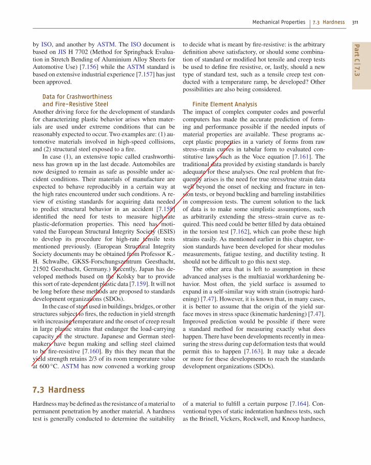
Data for Crashworthinessand Fire-Resistive Steel
Another driving force for the development of standardsfor characterizing plastic behavior arises when mater-ials are used under extreme conditions that can bereasonably expected to occur. Two examples are: (1) au-tomotive materials involved in high-speed collisions,and (2) structural steel exposed to a fire.
In case (1), an extensive topic called crashworthi-ness has grown up in the last decade. Automobiles arenow designed to remain as safe as possible under ac-cident conditions. Their materials of manufacture areexpected to behave reproducibly in a certain way atthe high rates encountered under such conditions. A re-view of existing standards for acquiring data neededto predict structural behavior in an accident [7.158]identified the need for tests to measure high-rateplastic-deformation properties. This need has moti-vated the European Structural Integrity Society (ESIS)to develop its procedure for high-rate tensile testsmentioned previously. (European Structural IntegritySociety documents may be obtained from Professor K.-H. Schwalbe, GKSS-Forschungszentrum Geesthacht,21502 Geesthacht, Germany.) Recently, Japan has de-veloped methods based on the Kolsky bar to providethis sort of rate-dependent plastic data [7.159]. It will notbe long before these methods are proposed to standardsdevelopment organizations (SDOs).
In the case of steel used in buildings, bridges, or otherstructures subject to fires, the reduction in yield strengthwith increasing temperature and the onset of creep resultin large plastic strains that endanger the load-carryingcapacity of the structure. Japanese and German steel-makers have begun making and selling steel claimedto be fire-resistive [7.160]. By this they mean that theyield strength retains 2/3 of its room temperature valueat 600 ◦C. ASTM has now convened a working group
to decide what is meant by fire-resistive: is the arbitrarydefinition above satisfactory, or should some combina-tion of standard or modified hot tensile and creep testsbe used to define fire resistive, or, lastly, should a newtype of standard test, such as a tensile creep test con-ducted with a temperature ramp, be developed? Otherpossibilities are also being considered.
Finite Element AnalysisThe impact of complex computer codes and powerfulcomputers has made the accurate prediction of form-ing and performance possible if the needed inputs ofmaterial properties are available. These programs ac-cept plastic properties in a variety of forms from rawstress–strain curves in tabular form to evaluated con-stitutive laws such as the Voce equation [7.161]. Thetraditional data provided by existing standards is barelyadequate for these analyses. One real problem that fre-quently arises is the need for true stress/true strain datawell beyond the onset of necking and fracture in ten-sion tests, or beyond buckling and barreling instabilitiesin compression tests. The current solution to the lackof data is to make some simplistic assumptions, suchas arbitrarily extending the stress–strain curve as re-quired. This need could be better filled by data obtainedin the torsion test [7.162], which can probe these highstrains easily. As mentioned earlier in this chapter, tor-sion standards have been developed for shear modulusmeasurements, fatigue testing, and ductility testing. Itshould not be difficult to go this next step.
The other area that is left to assumption in theseadvanced analyses is the multiaxial workhardening be-havior. Most often, the yield surface is assumed toexpand in a self-similar way with strain (isotropic hard-ening) [7.47]. However, it is known that, in many cases,it is better to assume that the origin of the yield sur-face moves in stress space (kinematic hardening) [7.47].Improved prediction would be possible if there werea standard method for measuring exactly what doeshappen. There have been developments recently in mea-suring the stress during cup deformation tests that wouldpermit this to happen [7.163]. It may take a decadeor more for these developments to reach the standardsdevelopment organizations (SDOs).
7.3 Hardness
Hardness may be defined as the resistance of a material topermanent penetration by another material. A hardnesstest is generally conducted to determine the suitability
of a material to fulfill a certain purpose [7.164]. Con-ventional types of static indentation hardness tests, suchas the Brinell, Vickers, Rockwell, and Knoop hardness,
PartC
7.3

312 Part C Measurement Methods for Materials Properties
Table 7.5 First publications of hardness testing standards in different countries
Test method Germany UK USA France ISO Europe
Brinell (1900) 1942 1937 1924 1946 1981 1955
Rockwell (1919) 1942 1940 1932 1946 1986 1955
Vickers (1925) 1940 1931 1952 1946 1982 1955
Knoop (1939) 1969 1993
����������� ���� �����
- ���������� ��= ;�;�, �8���� ������ >
9���� ���� "�� ����?���� ����"�� ���"���
�������@ ���������"�� ��"� � �������
� 5 � �#���������"�4��� �������� ����� ������������� ����� ��������#������
� �������������A �� 9���� ���+��� � &�� +��������0 !�������������������#� ���� B $�# �� �� � ����#��� ����# ����
5�� ���� �����
����������������������������������
/���� ���� �����
/�����# �� ����� ��������� ���!$��8�804���"� ��.��7 ���# �����9.�
����
5 � �#����������� �� ���"���
5&��#������� ���� �����
4 ���� # ���"� � ��&
9���� ���� "�� ����?���� ����"�� ���"���
����� � �����������"��
9���� ���� "�� �� &� �����"�� � �������
���� ��.��7 ��
-��7� ��-��7� ���=�#C�2#C��:#>4���"� ������ ���# �����9��
D����
D64'(B
5 � �#���������"� �� #�+����"�� ���"���
Fig. 7.26 Overview of the hardness testing methods. (see [7.165])
provide a single hardness number as the result, whichis most useful as it correlates to other properties of thematerial, such as strength, wear resistance, and ductility.The correlation of hardness to other physical propertieshas made it a common tool for industrial quality control,acceptance testing, and selection of materials.
With the rising interest in the testing of thin coatingsand in order to obtain more information from an inden-tation test, the instrumented indentation tests have beendeveloped and standardized. In addition to obtainingconventional hardness values, the instrumented indenta-tion tests can also determine other material parameterssuch as Martens hardness, indentation hardness, in-dentation modulus, indentation creep and indentationrelaxation.
Hardness testing is one of the longest used and well-known test methods not only for metallic materials,but for other types of material as well. It has special
importance in the field of mechanical test methods, be-cause it is a relative inexpensive, easy to use and nearlynondestructive method for the characterization of ma-terials and products. In order to work with comparablemeasured values, standards of hardness testing methodshave been developed. This work started in the 1920s(see Table 7.5). In some cases, national, regional andinternational standards specify different requirements;however, it is generally accepted to aim at the completealignment of hardness standards at all standardizationlevels [7.166, 167].
Hardness data are test-system dependent and notfundamental metrological values. For this reason, hard-ness testing needs a combination of certified referencematerials (reference blocks) and certified calibrationmachines to establish and maintain national and world-wide uniform hardness scales. Therefore, all hardnesstesting standards related to a specific hardness test
PartC
7.3

Mechanical Properties 7.3 Hardness 313
include different parts specifying requirements forthe:
1. Test method,2. Verification and calibration of testing machines, and3. Calibration of reference blocks.
An overview of the different well-known con-ventional methods of hardness testing is givenin Fig. 7.26.
7.3.1 Conventional Hardness Test Methods(Brinell, Rockwell, Vickers and Knoop)
The most commonly used indentation hardness testsused today are the Brinell, Rockwell, Vickers, andKnoop methods. Beginning with the introduction ofthe Brinell hardness test in 1900, these methods weredeveloped over the next four decades, each bringingan improvement to testing applications. The Rockwellmethod greatly increased the speed of testing for indus-try, the Vickers method provided a continuous hardnessscale from the softest to hardest metals, and the Knoopmethod provided greater measurement sensitivity at thelowest test forces. Since their development, these meth-ods have been improved and their applications expanded,particularly in the cases of the Brinell and Rockwellmethods.
��
�
�
��
��
Fig. 7.27 Principle of the Brinell hardness test
Many manufactured products are made of differenttypes of materials, varying in hardness, strength, sizeand thickness. To accommodate the testing of these di-verse products, each conventional hardness method hasdefined a range of standard force levels to be used in con-junction with several different types of indenters. Eachcombination of indenter type and applied force levelhas been designated as a distinct hardness scale of thespecific hardness test method.
Brinell Hardness Test (HBW)Principle of the Brinell Hardness Test [7.168, 169]. Anindenter (hardmetal ball with diameter D) is forced intothe surface of a test piece and the diameter of the in-dentation d left in the surface after removal of the forceF is measured (Fig. 7.27). The Brinell hardness is pro-portional to the quotient obtained by dividing the testforce by the curved surface area of the indentation. Theindentation is assumed to be spherical with a radiuscorresponding to half of the diameter of the ball
Brinell hardness HBW
= Constant ×Test force
Surface area of indentation
= 0.102 ×2F
πD(D −√D2 −d2)
, (7.24)
where F is in N and D and d are in mm.
Designation of the Brinell Hardness Test. The Brinellhardness is denoted by HBW followed by numbers rep-resenting the ball diameter, applied test force, and theduration time of the test force. Note that, in former stan-dards, in cases when a steel ball had been used, theBrinell hardness was denoted by HB or HBS.
Example. 600 HBW 1/30/20:
600 Brinell hardness valueHBW Brinell hardness symbol1/ Ball diameter in mm30 Applied test force (294.2 N = 30 kgf)/20 Duration time of test force (20 s) if not indicated
in the designation (10–15 s)
Application of the Brinell Hardness Test. For the appli-cation of the Brinell hardness test, the most commonlyused Brinell scales for different testing conditions aregiven in Table 7.6. Other combinations of test forces andball sizes are allowed, usually by special agreement.
PartC
7.3

314 Part C Measurement Methods for Materials Properties
Table 7.6 Standard test forces for the different testing conditions
Hardness symbol Ball diameter D (mm) Force:diameter ratio0.102F/D2 (N/mm2)
Nominal value of test forceF (kN)
HBW 10/3000 10 30 29.42
HBW 10/1500 10 15 14.71
HBW 10/1000 10 10 9.807
HBW 10/500 10 5 4.903
HBW 10/250 10 2.5 2.452
HBW 10/100 10 1 0.9807
HBW 5/750 5 30 7.355
HBW 5/250 5 10 2.452
HBW 5/125 5 5 1.226
HBW 5/62.5 5 2.5 0.6129
HBW 5/25 5 1 0.2452
HBW 2.5/187.5 2.5 30 1.839
HBW 2.5/62.5 2.5 10 0.6129
HBW 2.5/31.25 2.5 5 0.3065
HBW 2.5/15.62 2.5 2.5 0.1532
HBW 2.5/6.25 2.5 1 0.06129
HBW 1/30 1 30 0.2942
HBW 1/10 1 10 0.09807
HBW 1/5 1 5 0.04903
HBW 1/2, 5 1 2.5 0.02452
HBW 1/1 1 1 0.009807
Advantages of the Brinell Hardness Test.
• Suitable for hardness tests even under rough work-shop conditions if large ball indenters and high testforces are used.• Suitable for hardness tests on inhomogeneous mater-ials because of the large test indentations, providedthat the extent of the inhomogeneity is small incomparison to the test indentation.• Suitable for hardness tests on large blanks such asforged pieces, castings, hot-rolled or hot-pressed andheat-treated components.• Relatively little surface preparation is required iflarge ball indenters and high test forces are used.• Measurement is usually not affected by movementof the specimen in the direction in which the testforce is acting.• Simple, robust and low-cost indenters.
Disadvantages of the Brinell Hardness Test.
• Restriction of application range to a maximumBrinell hardness of 650 HBW.• Restriction when testing small and thin-walled spec-imens.
• Relatively long test time due to the measurement ofthe indentation diameter.• Relatively serious damage to the specimen due tothe large test indentation.• Measurement of many indentations can lead to op-erator fatigue and increased measurement error.
Rockwell Hardness Test (HR)Principle of the Rockwell Hardness Test [7.170,171]. Thegeneral Rockwell test procedure is the same regardlessof the Rockwell scale or indenter being used. The inden-ter is brought into contact with the material to be testedand a preliminary force is applied to the indenter. Thepreliminary force is held constant for a specified time du-ration, after which the depth of indentation is measured.An additional force is then applied at a specified rate toincrease the applied force to the total force level. Thetotal force is held constant for a specified time duration,after which the additional force is removed, returningto the preliminary force level. After holding the prelim-inary force constant for a specified time duration, thedepth of indentation is measured for a second time, fol-lowed by removal of the indenter from the test material(Fig. 7.28). The difference in the two depth measure-
PartC
7.3

Mechanical Properties 7.3 Hardness 315
E
�:
�
�
0
�
�:��� �:
F
B
Fig. 7.28 Rockwell principle diagram (Key: 1 – Indenta-tion depth by preliminary force F0; 2 – Indentation depthby additional test force F1; 3 – Elastic recovery just afterremoval of additional test force F1; 4 – Permanent indenta-tion depth h; 5 – Surface of test piece; 6 – Reference planefor measurement; 7 – Position of indenter)
ments is calculated as h in mm. From the value of hand the two constant numbers N and S (Table 7.7), theRockwell hardness is calculated following the formula:
Rockwell hardness = N − h
S. (7.25)
Designation of the Rockwell Hardness Test. The Rock-well hardness is denoted by the symbol HR, followedby a letter indicating the scale, and either an S or W toindicate the type of ball used (S = steel; W = hardmetal,tungsten carbide alloy) (Table 7.7).
Example. 70 HR 30N W:
70 Rockwell hardness valueHR Rockwell hardness symbol30N Rockwell scale symbol (Table 7.7)W Indication of type of ball used, S = steel, W = hard-
metal
Application of the Rockwell Hardness Test. For theapplication of the Rockwell hardness test, the indentertypes and specified test forces, as well as, typical appli-cations for the different scales are given in Table 7.7.ASTM International defines thirty different Rockwellscales [7.170] while the ISO [7.171] defines a subset ofthese scales (Table 7.7).
Advantages of the Rockwell Hardness Test.
• Relatively short test time because the hardness valueis automatically displayed immediately followingthe indentation process.• The test may be automated.• Relatively low procurement costs for the testingmachine because no optical measuring device isnecessary.• No operator influence of evaluation because thehardness value is displayed directly.• Relatively short time needed to train operator.
Disadvantages of the Rockwell Hardness Test.
• Possibility of measurement errors due to movementof the test piece and poorly seated or worn machinecomponents during the application of the test forces.• Less possibility of testing materials with surfacelayer hardening as a consequence of relatively hightest forces.• Sensitivity of the diamond indenter to damage, thusproducing a risk of incorrect measurements• Relatively low sensitivity on the difference in hard-ness.• Significant influence of the shape of the conical di-amond indenter on the test result (especially of thetip).
Vickers Hardness Test (HV)Principle of the Vickers Hardness Test [7.172–174]. A di-amond indenter in the form of a right pyramid witha square base and with a specified angle between oppo-site faces at the vertex is forced into the surface of a testpiece followed by measurement of the diagonal lengthof the indentation left in the surface after removal of thetest force F (Fig. 7.29).
Designation of the Vickers Hardness Test. The Vickershardness is denoted by the symbol HV followed by num-bers representing the applied test force, and the durationtime of the test force.
Example. 640 HV 30/20:
640 Vickers hardness valueHV Hardness symbol30 Applied test force (294.2 N = 30 kgf)/20 Duration time of test force (20 s) if not indicated in
the designation (10–15 s)
PartC
7.3

316 Part C Measurement Methods for Materials Properties
Table 7.7 Rockwell hardness scales and typical applications [7.175]
Scalesymbol
Indenter type(ball dimensions
Preliminaryforce
Totalforce
Typical applications HR calculation
indicate diameter) (N) (N) N S
HRA Spheroconicaldiamond
98.07 588.4 Cemented carbides, thin steel, and shallow case hard-ened steel
100 0.002
HRB Ball – 1.588 mm 98.07 980.7 Copper alloys, soft steels, aluminum alloys, malleableiron, etc.
130 0.002
HRC Spheroconicaldiamond
98.07 1471 Steel, hard cast irons, pearlitic malleable iron, tita-nium, deep case hardened steel, and other materialsharder than HRB 100
100 0.002
HRD Spheroconicaldiamond
98.07 980.7 Thin steel and medium case hardened steel, andpearlitic malleable iron
100 0.002
HRE Ball – 3.175 mm 98.07 980.7 Cast iron, aluminum and magnesium alloys, and bear-ing metals
130 0.002
HRF Ball – 1.588 mm 98.07 588.4 Annealed copper alloys, and thin soft sheet metals 130 0.002
HRG Ball – 1.588 mm 98.07 1471 Malleable irons, copper–nickel–zinc and cupro–nickelalloys
130 0.002
HRH Ball – 3.175 mm 98.07 588.4 Aluminum, zinc, and lead 130 0.002
HRK Ball – 3.175 mm 98.07 1471 Bearing metals and other very soft or thin materials, 130 0.002
HRLa Ball – 6.350 mm 98.07 588.4 use smallest ball and heaviest load that does not give 130 0.002
HRMa Ball – 6.350 mm 98.07 980.7 anvil effect 130 0.002
HRPa Ball – 6.350 mm 98.07 1471 130 0.002
HRRa Ball – 12.70 mm 98.07 588.4 130 0.002
HRSa Ball – 12.70 mm 98.07 980.7 130 0.002
HRVa Ball – 12.70 mm 98.07 1471 130 0.002
HR15N Spheroconicaldiamond
29.42 147.1 Similar to A, C and D scales, but for thinner gagematerial or case depth
100 0.001
HR30N Spheroconicaldiamond
29.42 294.2 100 0.001
HR45N Spheroconicaldiamond
29.42 441.3 100 0.001
HR15T Ball – 1.588 mm 29.42 147.1 Similar to B, F and G scales, but for thinner gage 100 0.001
HR30T Ball – 1.588 mm 29.42 294.2 material 100 0.001
HR45T Ball – 1.588 mm 29.42 441.3 100 0.001
HR15Wa Ball – 3.175 mm 29.42 147.1 Very soft material 100 0.001
HR30Wa Ball – 3.175 mm 29.42 294.2 100 0.001
HR45Wa Ball – 3.175 mm 29.42 441.3 100 0.001
HR15Xa Ball – 6.350 mm 29.42 147.1 100 0.001
HR30Xa Ball – 6.350 mm 29.42 294.2 100 0.001
HR45Xa Ball – 6.350 mm 29.42 441.3 100 0.001
HR15Ya Ball – 12.70 mm 29.42 147.1 100 0.001
HR30Ya Ball – 12.70 mm 29.42 294.2 100 0.001
HR45Ya Ball – 12.70 mm 29.42 441.3 100 0.001a These scales are defined by ASTM International, but are not included in the ISO standards
Application of the Vickers Hardness Test. ISO [7.174]specifies the method of Vickers hardness test forthe three different ranges of test force for metal-
lic materials, whereas ASTM International [7.172,173] divides the Vickers test into two ranges (Ta-ble 7.8).
PartC
7.3
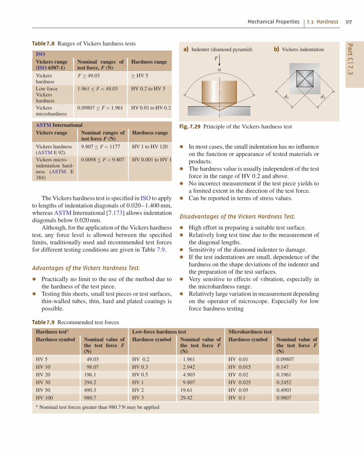
Mechanical Properties 7.3 Hardness 317
Table 7.8 Ranges of Vickers hardness tests
ISO
Vickers range(ISO 6507-1)
Nominal ranges oftest force, F (N)
Hardness range
Vickershardness
F ≥ 49.03 ≥ HV 5
Low forceVickershardness
1.961 ≤ F < 49.03 HV 0.2 to HV 5
Vickersmicrohardness
0.09807 ≤ F < 1.961 HV 0.01 to HV 0.2
ASTM International
Vickers range Nominal ranges oftest force F (N)
Hardness range
Vickers hardness(ASTM E 92)
9.807 ≤ F < 1177 HV 1 to HV 120
Vickers micro-indentation hard-ness (ASTM E384)
0.0098 ≤ F < 9.807 HV 0.001 to HV 1
The Vickers hardness test is specified in ISO to applyto lengths of indentation diagonals of 0.020–1.400 mm,whereas ASTM International [7.173] allows indentationdiagonals below 0.020 mm.
Although, for the application of the Vickers hardnesstest, any force level is allowed between the specifiedlimits, traditionally used and recommended test forcesfor different testing conditions are given in Table 7.9.
Advantages of the Vickers Hardness Test.
• Practically no limit to the use of the method due tothe hardness of the test piece.• Testing thin sheets, small test pieces or test surfaces,thin-walled tubes, thin, hard and plated coatings ispossible.
Table 7.9 Recommended test forces
Hardness testa Low-force hardness test Microhardness test
Hardness symbol Nominal value ofthe test force F(N)
Hardness symbol Nominal value ofthe test force F(N)
Hardness symbol Nominal value ofthe test force F(N)
HV 5 49.03 HV 0.2 1.961 HV 0.01 0.09807
HV 10 98.07 HV 0.3 2.942 HV 0.015 0.147
HV 20 196.1 HV 0.5 4.903 HV 0.02 0.1961
HV 30 294.2 HV 1 9.807 HV 0.025 0.2452
HV 50 490.3 HV 2 19.61 HV 0.05 0.4903
HV 100 980.7 HV 3 29.42 HV 0.1 0.9807a Nominal test forces greater than 980.7 N may be applied
�
�
/�� �� ��=���#�����&��#��>�� .��7 ������ ���������
� �
Fig. 7.29 Principle of the Vickers hardness test
• In most cases, the small indentation has no influenceon the function or appearance of tested materials orproducts.• The hardness value is usually independent of the testforce in the range of HV 0.2 and above.• No incorrect measurement if the test piece yields toa limited extent in the direction of the test force.• Can be reported in terms of stress values.
Disadvantages of the Vickers Hardness Test.
• High effort in preparing a suitable test surface.• Relatively long test time due to the measurement ofthe diagonal lengths.• Sensitivity of the diamond indenter to damage.• If the test indentations are small, dependence of thehardness on the shape deviations of the indenter andthe preparation of the test surfaces.• Very sensitive to effects of vibration, especially inthe microhardness range.• Relatively large variation in measurement dependingon the operator of microscope. Especially for lowforce hardness testing
PartC
7.3

318 Part C Measurement Methods for Materials Properties
Table 7.10 Symbols and designations for the Knoop hardness test
Symbol Designation
F Test force (N)
d Length of the long diagonal (mm)
c Indenter constant, relating projected area of the indentation to the square of the length of the long diagonal
Indenter constant, c = tan β2
2 tan α2
, ideally c = 0.07028,
where α and β are the angles between the opposite edges at the vertex of the diamond pyramid (Fig. 7.30)
HK
Knoop hardness = Gravitational constanta ×Test force
Projected area of indentation
= 0.102 ×F
cd2= 1.451
F
d2
a: gravitational constant = 1
gn= 1
9.80665≈ 0.102, where gn is the acceleration of gravity
For the application of the Vickers hardness test for thedifferent ranges of test force see [7.176–179].
Knoop Hardness Test (HK)Principle of the Knoop Hardness Test [7.173,180]. A di-amond indenter, in the form of a rhombic-based pyramidwith specified angles between opposite faces at the ver-tex, is forced into the surface of a test piece followed bymeasurement of the long diagonal of the indentation re-maining in the surface after removal of the test force F(Figs. 7.30, 7.31, Table 7.10).
The Knoop hardness is proportional to the quotientobtained by dividing the test force by the projected areaof the indentation, which is assumed to be a rhombic-based pyramid, and having at the vertex the same anglesas the indenter.
�
�� �
Fig. 7.30 Symbols and designations for the Knoop hardnesstest
Designation of the Knoop Hardness. The Knoop hard-ness is denoted by the symbol HK followed by numbersrepresenting the applied test force, and the duration timeof the test force.
Example. 640 HK 0.1/20:
640 Knoop hardness valueHK Hardness symbol0.1 Applied test force (0.9807 N = 0.1 kgf)/20 Duration time of test force (20 s) if not indicated in
the designation (10–15 s)
Application of the Knoop Hardness Test. For the appli-cation of the Knoop hardness test, traditionally used andrecommended test forces for different testing conditionsare given in Table 7.11.
Advantages of the Knoop Hardness Test.
• Particularly suitable for narrow test pieces, suchas wire, due to the large diagonal length ratio ofapproximately 7 : 1.
��#�#�);
3
3
Fig. 7.31 Symbols and designations for the Knoop hardnesstest
PartC
7.3

Mechanical Properties 7.3 Hardness 319
Table 7.11 Recommended test forces
Hardness Symbol Nominal value of the testforce F (N)
HK 0.01 0.09807
HK 0.02 0.1961
HK 0.025 0.2452
HK 0.05 0.4903
HK 0.1 0.9807
HK 0.2 1.961
HK 0.3 2.942
HK 0.5 4.903
HK 1 9.807
• Better suited to thin test pieces or platings than theVickers test method because the indentation depthis smaller by a factor of four for the same diagonallength.• Particularly suitable for brittle materials because oflower tendency to cracking.• Particularly suited to investigating the anisotropy ofa material because the Knoop test is dependent onthe direction selected for the long diagonal in suchcases.• In most cases, the small indentation has no influenceon the function or appearance of tested materials orproducts.• Practically no limit on the application of the methodfrom the hardness of the material tested.
Disadvantages of the Knoop Hardness Test.
• Time effort to achieve a sufficiently fine test surface.• Considerable dependency of the hardness on thetest force, with an especially strong influence of thepreparation of the test surface.• Sensitivity to damage of the diamond indenter.• Expensive alignment of the test surface to achievesymmetrical test indentations.• Relatively long test time due to the measurement ofthe diagonal length.• Measurement of the diagonal length is more difficultthan in the Vickers test method as a consequence ofthe indenter geometry.
7.3.2 Selecting a Conventional HardnessTest Method and Hardness Scale
The selection of a specific hardness testing methodis substantially influenced by many factors as dis-cussed below. Unfortunately, there is no one hardness
test that meets the optimum conditions for all appli-cations. Although the Brinell, Rockwell, Vickers andKnoop hardness testing methods have been developedto be capable of testing most materials, in many test-ing circumstances the size or depth of the indentation isgenerally the primary consideration when choosing theappropriate test forces and type of indenter to be uti-lized by the hardness test method. The combinations oftest forces and indenter types are known as a hardnessmethod’s specific hardness scales. The hardness scaleshave been defined to provide suitable measurement sen-sitivity and indentation depths that are appropriate fordifferent materials, strengths and dimensions of testpieces. The largest and deepest indentations are gen-erally obtained from the heavy-force Brinell scales,followed by the commonly used heavy-force Rockwelland Vickers scales, while small to extremely small in-dentations can be obtained from the commonly usedlower-force Rockwell, Vickers and Knoop scales.
Strength of the Test PieceA material’s resistance to penetration or its strength is ofprimary importance when selecting a hardness methodor hardness scale. An appropriate test force and indentermust be chosen to produce a large enough indentationin the test material to enable the hardness testing ma-chine’s measuring system to resolve and measure thedepth or size of the indentation with sufficient sensitiv-ity to produce a meaningful hardness result, but at thesame time to not penetrate too deeply beyond the inden-ter’s useful depth. On the other hand, a suitable indenterof the appropriate material, size and shape must be cho-sen to prevent the indenter from being damaged whentesting high-strength materials. For example, hardenedand tempered steel material generally requires hardnessmethods that employ higher test forces and a pointed orconical diamond indenter, whereas testing cemented car-bides with high forces could lead to the diamond beingfractured.
Test-Piece Size, Shape, Weight, Accessibility,Dimensions, and Thickness
The choice of a hardness test method may be influencedby the size, shape or weight of the test piece. The designsof some typical standard hardness testing machines mayprevent the testing of very large and heavy test piecesor unusually shaped test pieces, and may require specialmachine designs, special designs of indenters or addi-tional test piece support fixtures. These types of designsare usually limited to the Brinell, Rockwell and heavy-force Vickers machines. In contrast, small sample sizes
PartC
7.3

Mechanical Properties 7.4 Strength 333
(≈ 80–100 mN for an average radius Berkovich tipindenting fused silica).
Principle. The total measured compliance CT is the sumof contact compliance Cs and the machine complianceCf thus:
CT = Cs +Cf , (7.35)
where CT is derived from the derivative of the (uncor-rected) test force removal curve at maximum force
CT =( dF
dh
)−1(7.36)
and Cs is the contact compliance of the specimen ma-terial
Cs =√
π
2Er· 1√
AP(hc)(7.37)
with1
Er= 1−νs
EIT+ 1−νi
Ei(7.38)
and
hc = hmax − ε FmaxCT , (7.39)
where Ei and νi are, respectively, the Young’s modulusand the Poisson number of the indenter.
Thus the total compliance is
CT = Cf +√
π
2Er
1√
Ap(hc). (7.40)
If it can be assumed that the elastic modulus is constantand independent of indentation depth, a plot of CT ver-sus A−1/2 is linear for a given material and the intercept
of the plot is a direct measure of the machine load-framecompliance. The best values of Cf are obtained whenthe second term on the right-hand side of (7.39) is small,i. e., for large indentations. In addition, the largest inden-tations are advantageous to find area function. A perfectmodified Berkovich indenter, for instance
A(hc) = 24.5h2c (7.41)
can be used to provide a first estimate of the contactarea. Initial estimations of Cf and Er are thus obtained byplotting CT versus A−1/2 for the two largest indentationsin the reference block. Using these values, contact areasare computed for all, at least six, indentation sizes byrewriting (7.39) as
AP = π
4
1
E2r
1
(C −Cf)2 , (7.42)
from which an initial guess at the area function is madeby fitting Ap versus hc data to the relationship
A(hc)P = 24.5h2c +C1h1
c +C2h1/2c
+C3h1/4c +· · ·+C8h1/128
c , (7.43)
where C1–C8 are constants. The lead term describesa perfect modified Berkovich indenter; the others de-scribe deviations from the Berkovich geometry due toblunting of the tip.
The procedure is not complete at this stage becausethe exact form of the area function influences the valuesof Cf and Er, so using the new area function the pro-cedure shall be applied again and iterated several timesuntil convergence is achieved.
7.4 Strength
The strength of materials is influenced by the strainrate, temperature, loading manner and chemical envi-ronment. The conventional test for the examination ofthe strength of materials is tension testing with a slowstrain rate of around 10−3 s−1 at room temperature. Ten-sile properties obtained using this test are widely used inengineering practices such as mechanical design, fabri-cation and maintenance of products. In the case of brittlematerials, compression or bending tests are frequentlyused to examine their strength. These tests are doneunder so-called quasistatic-loading conditions. Tests atvery slow strain rates are performed to examine creep orstress-relaxation behavior. To consider automobile col-lision, earthquakes etc., strength at a high strain rate
such as 103 s−1 is required; impact or high-speed de-formation testing, such as a Hopkinson pressure-bartest, is employed. Resistance to fracture under cyclicloading is called fatigue strength. Strength is also in-fluenced by temperature as well as the environmentaccompanied by chemical reactions such as corrosion,or radiation damage. Fracture is frequently found to oc-cur under combined conditions of stress, microstructuralchange and chemical reaction. In some cases, high-temperature strength or low-temperature toughness areof importance for engineering application of mater-ials, so that the meaning of the strength of materialsis not unique but depends on the conditions of theiruse.
PartC
7.4
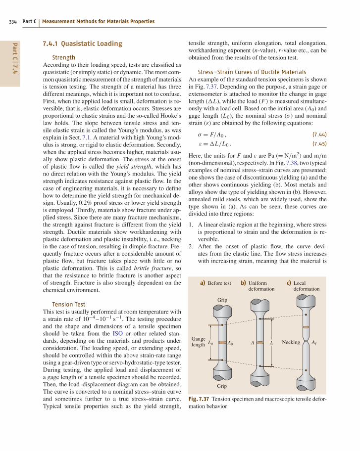
334 Part C Measurement Methods for Materials Properties
7.4.1 Quasistatic Loading
StrengthAccording to their loading speed, tests are classified asquasistatic (or simply static) or dynamic. The most com-mon quasistatic measurement of the strength of materialsis tension testing. The strength of a material has threedifferent meanings, which it is important not to confuse.First, when the applied load is small, deformation is re-versible, that is, elastic deformation occurs. Stresses areproportional to elastic strains and the so-called Hooke’slaw holds. The slope between tensile stress and ten-sile elastic strain is called the Young’s modulus, as wasexplain in Sect. 7.1. A material with high Young’s mod-ulus is strong, or rigid to elastic deformation. Secondly,when the applied stress becomes higher, materials usu-ally show plastic deformation. The stress at the onsetof plastic flow is called the yield strength, which hasno direct relation with the Young’s modulus. The yieldstrength indicates resistance against plastic flow. In thecase of engineering materials, it is necessary to definehow to determine the yield strength for mechanical de-sign. Usually, 0.2% proof stress or lower yield strengthis employed. Thirdly, materials show fracture under ap-plied stress. Since there are many fracture mechanisms,the strength against fracture is different from the yieldstrength. Ductile materials show workhardening withplastic deformation and plastic instability, i. e., neckingin the case of tension, resulting in dimple fracture. Fre-quently fracture occurs after a considerable amount ofplastic flow, but fracture takes place with little or noplastic deformation. This is called brittle fracture, sothat the resistance to brittle fracture is another aspectof strength. Fracture is also strongly dependent on thechemical environment.
Tension TestThis test is usually performed at room temperature witha strain rate of 10−4 –10−1 s−1. The testing procedureand the shape and dimensions of a tensile specimenshould be taken from the ISO or other related stan-dards, depending on the materials and products underconsideration. The loading speed, or extending speed,should be controlled within the above strain-rate rangeusing a gear-driven type or servo-hydrostatic-type tester.During testing, the applied load and displacement ofa gage length of a tensile specimen should be recorded.Then, the load–displacement diagram can be obtained.The curve is converted to a nominal stress–strain curveand sometimes further to a true stress–strain curve.Typical tensile properties such as the yield strength,
tensile strength, uniform elongation, total elongation,workhardening exponent (n-value), r-value etc., can beobtained from the results of the tension test.
Stress–Strain Curves of Ductile MaterialsAn example of the standard tension specimens is shownin Fig. 7.37. Depending on the purpose, a strain gage orextensometer is attached to monitor the change in gagelength (ΔL), while the load (F ) is measured simultane-ously with a load cell. Based on the initial area (A0) andgage length (L0), the nominal stress (σ) and nominalstrain (ε) are obtained by the following equations:
σ = F/A0 , (7.44)
ε = ΔL/L0 . (7.45)
Here, the units for F and ε are Pa (= N/m2) and m/m(non-dimensional), respectively. In Fig. 7.38, two typicalexamples of nominal stress–strain curves are presented;one shows the case of discontinuous yielding (a) and theother shows continuous yielding (b). Most metals andalloys show the type of yielding shown in (b). However,annealed mild steels, which are widely used, show thetype shown in (a). As can be seen, these curves aredivided into three regions:
1. A linear elastic region at the beginning, where stressis proportional to strain and the deformation is re-versible.
2. After the onset of plastic flow, the curve devi-ates from the elastic line. The flow stress increaseswith increasing strain, meaning that the material is
(���
��
(���
� �7���(��� � ����
� "�� �� �� �� !��"��#� "��#�����
�� ,����� "��#�����
�:�: � � �"
Fig. 7.37 Tension specimen and macroscopic tensile defor-mation behavior
PartC
7.4

Mechanical Properties 7.4 Strength 335
��#�����������
��#�������� ����
6����������
�
,�� ��� ���
��!
�� ��,
��
�2
��#�����������
��#�������� ����
6����������
�
!��"��#� ���������
��
�2
��
�:;�
:;�<
,���� ���������
Fig. 7.38a,b Nominal stress–strain curves: (a) discontinu-ous yielding and (b) continuous yielding
strengthened by plastic deformation; this is calledworkhardening. When unloaded, only the elasticstrain is recovered but a permanent deformation,i. e., plastic strain, remains. In this region, uniformplastic deformation occurs. For plastic strains, thecondition of constant volume is often assumed. Fig-ure 7.37b [7.206].
3. After reaching the maximum stress, which is calledthe ultimate tensile strength (UTS) or simply the
��
:
�: �# �� �:: �# �� �:: �#
Fig. 7.39a–c Fracture surface:(a) dimple, (b) cleavage and(c) intergranular fracture
tensile strength (TS), a lower stress is enough tocontinue to deform the material plastically becausenecking occurs (Fig. 7.37c). After the onset of neck-ing, deformation is localized to a necked region inwhich the stress condition is no longer uniaxial but istriaxial. Microvoids form inside the necked region,grow, connect to each other and lead to slip-off ofthe remaining, outside ring region. Thus, the viewafter fracture looks like a cup and a cone and henceis called cup-and-cone fracture. This phenomenonis typical of ductile fracture. The inner, flat area con-sists of dimples; the dimple pattern observed on thefracture surface is shown in Fig. 7.39a.
4. When a material is brittle, as is the case for ceramics,necking is not observed and the flow curve stops sud-denly at the fracture stress, often within the elasticregime. In such a case, the fracture surface con-sists of cleavage or transgranular facets. Examplesof these fracture surface are presented in Figs. 7.39band 7.39c,
True Stress–Strain Curves and theWorkhardening Exponent (n-Value)
Within the uniformly elongated regime in Fig. 7.38, theassumption of constant volume for plastic strains holdsapproximately. This means that the cross section in thegage volume in Fig. 7.37 decreases with increasing ten-sile strain. Hence, the area (A) to support the appliedstress decreases with deformation so that the stress perunit area is given by
σ∗ = F/A (7.46)
instead of (7.44); σ∗ is called the true stress. Similarlyto σ∗, the gage length l0 changes continuously withdeformation. Then, the true strain (ε∗) is defined by
ε∗ =l∫
l0
dl/l = ln(l/l0) . (7.47)
PartC
7.4

336 Part C Measurement Methods for Materials Properties
��
�
��
��
��
Fig. 7.40 Stress condition in a necked region in tension test
One of the merits of using ε∗ is its additive nature.For instance, when a length changes from LA to LB,and then to LC, the true strain from LA to LB isln(LB/LA) and from LB to LC is ln(LC/LB). There-fore, ln(LB/LA)+ ln(LC/LB) = ln(LC/LA) holds. Incontrast, in the case of nominal strain, we have (LB −LA)/LA + (LC − LB)/LB = (LC − LA)/LA, and hencethis property is not additive. Taking the assumption ofconstant volume (A0L0 = AL) we obtain the followingconversion from nominal stress and strain to true stressand strain. Thus, we find the relation for true stress versustrue strain starting from Fig. 7.38 by using
σ∗ = F/A0 = σ(1+ ε) , (7.48)
ε∗ = ln(L/L0) = ln(1+ ε) . (7.49)
After the onset of necking, the specimen geometrychanges and the stress condition is also altered. Asshown in Fig. 7.37c and Fig. 7.40, the stress conditionin a necked region is not uniform but is a complicatedtriaxial stress condition. According to Bridgman’s analy-sis [7.207], the tensile stress at the surface of the smallestcross section, σ0 (Fig. 7.40), is given by
σ0 = F/A
(1+2R/a) ln(1+a/2R), (7.50)
where R and a are given in Fig. 7.40. Microvoids formin the center of the necked region under triaxial stresses,as explained above, leading to cup-and-cone fracture.
An example of curves of true stress versus true strainconverted from the nominal stress–strain curve by us-ing (7.49) and (7.50) is shown in Fig. 7.41. This shows
::
��#���������������� �������
��#�������� ����� ���� ���=4��>
�::
0::
F::
H::
�:::
��::
: :;0:;� :;� :;�
*��7%���� �������
��#�������� �����#�����������
�� ���� ������ �������
Fig. 7.41 True stress–strain curve in which the workhard-ening rate is plotted to indicate the onset of necking
that workhardening continues even in local deforma-tion; the necking is caused from the balance betweencross-sectional area reduction and workhardening withincreasing tensile plastic strain. Hence, the crossingpoint of the true stress σ∗ and the workhardening ratedσ∗/dε∗ shows the onset of necking (Fig. 7.41).
Tensile PropertiesTension testing is simple and gives us lots of useful in-formation on mechanical properties. So, this test is themost basic and popular to understand the mechanical be-havior of materials. Several parameters for engineeringuse obtained by tension testing are explained below.
Elastic Limit and Proportional LimitMost mechanical products are designed to be used withinthe regime of elastic deformation. The rigorous limit ofelastic deformation is determined by the elastic limit orproportional limit on the stress–strain curve. The pro-portional limit is the point of deviation from the linearrelationship between stress and strain. On the other hand,the elastic limit is found as the maximum stress with-out permanent strain after unloading. These stresses arevery sensitive to the method used to measure strain.Within the linear stress–strain regime, as was explainedin details in Sect. 7.1, the Young’s modulus (E) is de-termined from the slope, while the Poisson’s ratio (ν) isdetermined by the absolute ratio between the transversestrain and tensile strain. When the tensile direction istaken as the x3-axis, these are determined by
E = σ33/ε33 , (7.51)
ν = |ε11/ε33 | = |ε22/ ε33 | . (7.52)
PartC
7.4

Mechanical Properties 7.4 Strength 337
In the case of steel, E is nearly 200 GPa and ν is ap-proximately 0.3. The elastic strain in steels is usuallyless than 1%, which is very small compared with theuniform elongation of the order of 10%. We note herethat the constant-volume assumption is not applicable toelastic deformation.
Yield StrengthSpecial measurements such as those based on straingages are required for the measurement of elastic strainsless than 0.01 so that the yield strength (YS) is de-termined for mechanical design using the conventionaltensile test. In the case of discontinuous yielding ob-served in mild steel, as shown in Fig. 7.38a, the upper orlower yield point is observed on the stress–strain curveand used as the yield strength in engineering. After theupper yield point, a plastic-deformation regime calledthe Luders band appears and spreads within the speci-men gage volume under the lower yield stress. Since theupper yield strength is strongly dependent on the ten-sile speed, i. e., the strain rate, the lower yield strengthis more popularly used. The strain during this hetero-geneous deformation is called the Luders elongation,which is also dependent on grain size.
On the other hand, Fig. 7.38b shows the case of con-tinuous yielding, which is observed in many metals andalloys such as aluminum, austenitic stainless steel etc.0.2% proof stress is usually employed, which meansa plastic (permanent) strain of 0.2% remains after un-loading. Usually the elastic linear line is shifted by 0.2%and the intersection with the stress–strain curve is found.Macroscopic yielding can be observed to take place atthis point. Although 0.2% strain is the choice for engi-neering, other strains, for instance 0.1%, are employedin other industrial fields.
Tensile StrengthThe maximum stress appearing in Fig. 7.38 is deter-mined by the tensile strength (TS), frequently called theultimate tensile strength (UTS). In the case of an ex-treme design that allows plastic flow, TS is employed asthe design strength.
DuctilityParameters to describe the ductility includes uniformelongation, total elongation and reduction in area af-ter fracture. Uniform elongation is important for plasticforming etc. and is determined as the strain at the tensilestrength. After the tensile strength, local deformation,i. e. necking, starts. The total strain is given as thestrain to fracture in Fig. 7.41. It should be noted that
the total elongation is dependent on the gage lengthadopted. Therefore, fracture strain (εf) is sometimesused, which is defined as ln(A0/Af), where Af refersto the smallest area in the necked region after frac-ture. Conventionally, the reduction in area (ϕ) definedby [(A0 − Af)/A0]× 100% is used. The extreme caseobserved in a pure metal is a point fracture, whereAf = 0.
Workhardening Exponent (n-Value)The true stress–strain curve shown in Fig. 7.41 is oftenfitted by using the following Hollomon’s equation:
σ∗ = K (ε∗)n , (7.53)
where K and n stand for the strengthening factor and theworkhardening exponent (n-value), respectively. By tak-ing two measuring points or by using the least-squaresmethod for ln σ∗ versus ln ε∗ within an appropriate strainregime, these K and n values are determined. The n-value is important because it is equivalent with uniformelongation. The plastic instability condition, i. e., theonset of necking can be given by
dF = σ∗ dA + A dσ∗ = 0 , (7.54)
where F is the applied tensile load. This equationis rewritten by σ∗ = dσ∗/dε∗ under the assumptionof constant volume and therefore ε∗ = n is obtained.A large n-value means excellent plastic formability.
Rankford Value (Plastic Anisotropy: r-Value)Another parameter that indicates the plastic formability,and which is also obtained by the tension test for sheetmetals and alloys, is the r-value. When tensile strainreaches 10–20%, the strain for a thickness of εt and thestrain for a width of εw are measured and the r-value isdetermined by
r = εw/εt . (7.55)
If the assumption of constant volume is used, this be-comes
r = ln(W0/W )/ ln(LW/L0W0) , (7.56)
where W0, L0 and W , L refer to the width and gagelength in the tensile direction before and after the tensiontest, respectively. These values are much more easilymeasured precisely than the thickness because mostcases use thin sheets. In an isotropic material, the r-valueequals unity. Commercially available materials gener-ally show anisotropic feature in plastic flow because oftheir texture. Materials with high r-values are desirable
PartC
7.4

338 Part C Measurement Methods for Materials Properties
for heavy drawing because the thickness change is small.To achieve this, texture control is important.
The Compression TestThe compression test looks like the reverse of the ten-sion test, but more skill is required to obtain reliablestress–strain curves. A schematic illustration of com-pression of a round column is presented in Fig. 7.42,where the top and bottom surfaces of the specimenshould be maintained with good parallelism. Frictionbetween the specimen and the anvil must be minimizedusing an appropriate lubricant such as graphite or Mo2Spowder otherwise bulging, shown in Fig. 7.42b, becomesserious and leads to constrained deformation. If the com-pression alignmanet is not satisfactory with respect tothe specimen axis, buckling or bending occurs easily atsmall strains. To avoid such buckling, the length of thespecimen should be designed taking the cross-sectional
���
���
Fig. 7.42 Compression test where bulging is illustrated
��#���������������� �������
��#�������� ������� ���� ��
��#�������� ������#����������=� �����>
�� ���� ������ �������
��#�������� �����#������������=��#�� ������>
Fig. 7.43 Compression flow curve compared with that intension
area into consideration. Usually, the ratio of the diameterof the cross-sectional area d0 to the length h0 is chosenas 1.0–3.0. When the top and bottom of a specimen areplastically constrained by an anvil, the stress distributionwithin the cross section is not uniform and plastic defor-mation occurs in an inhomogeneous manner within thespecimen.
The nominal stress–strain curve obtained by thecompression test is higher than that obtained by the ten-sion test because the cross-sectional area increases withdeformation. Hence, flow curves measured by the ten-sion test and the compression test should be comparedin terms of true stress–strain curves. If a material showsisotropic plastic deformation, these two flow curves (thetrue stress–strain curves) coincide, as shown in Fig. 7.43.However, if a material contains phase or intergranularresidual stress, so-called second-type residual stresses,the yield strength will differ between compression andtension, which is called the strength difference (SD) ef-fect. The SD effect is also caused by crystallographicfeatures in plastic flow or stress-induced martensitictransformations.
In general, the flow stress (true stress) in compres-sion after some amount of tensile plastic deformationis smaller than that for continuous tension, as shownin Fig. 7.44. This is called the Baushinger effect (BE).As seen in Fig. 7.44, the magnitude of the BE is oftenexpressed by the BE stress or BE strain (Fig. 7.44). Gen-erally speaking, the flow stress becomes smaller whenthe strain path changes, even under biaxial or triaxialstresses. In a stress space (the general stress conditionis described by six components, as will be describedlater), the yield condition is shown using the yielding
GF::
�� �������
�� ���� ���=4��>
G�::
:
�::
F::
:;:�: :;::B :;:� :;:�B
�����
$�#�� �����
�����
:;::�
:;B��
�:;B
- �������
��
�-
Fig. 7.44 Tension-compression test to examine theBauschinger effect (BE) in which the parameters of BEstress (σP −σR) and BE strain β0.5 are defined
PartC
7.4

Mechanical Properties 7.4 Strength 339
surface. When a material is plastically deformed and thusworkhardened, the yielding stress surface expands andmoves in the stress space. Hence, the yield strength afterplastic deformation depends on the loading conditions.Typical cases are: (1) isotropic hardening, where theyield surface expands homogeneously, and (2) kinematichardening, where the surface moves without changingits shape and size. The BE is important in order to under-stand plastic forming, which is used to make mechanicalparts. In addition, the BE behavior is closely related tolow-cycle fatigue behavior. In the case of brittle mater-ials such as concrete, in which the SD effect for fractureis remarkable, the compressive fracture strength is muchhigher than the tensile value.
Hardness Test and Strength/Hardness RelationsIn addition to the treatment of hardness measurementsmethods given in Sect. 7.3, relations between strengthand hardness are briefly considered. The most popu-lar measurement is a kind of compression test with anindenter. The indenter is made from a hard materialsuch as diamond or high-carbon martensite steel. As ex-plained above and shown again in Fig. 7.45 an indenteris pressed on the surface of a testing material, and the in-dentation after unloading is measured. Since the Vickershardness test employs a pyramidal diamond indenter, theapplied stress is almost proportional to the area, whichmeans that the Vickers hardness number is insensitiveto the applied load. As is estimated in Fig. 7.45, thedeformation zone is limited to just underneath of theindenter and is complicated. According to an elasto–plastic analysis, the representative plastic strain in theplastic zone is about 8%, so that the hardness number
::
.��7 �������� ���9.
�::
0::
F::
H::
�:::
���� ������� ��
9�
:
�:
0:
F:
H:
�::
-��7� ������� ��
9-
:
�
���� ��� ����=(��>
��
F::
.��7 ������� ��
9.
��
:;B
�
�;B
�:: 0:: F:: H:: �:::
9-�
9-$
9�
��
:;0 :;H �;� �;F �::;� <�����"���� ���=(��>
�::
�::
�::
0::
B::
Fig. 7.46 Relationship between hardness and tensile properties
��
�� ��# �����"��
���� ���� �� �� .��7 ���� ��
$������ ������"��� ��# �
$������ ������"��� ��# �
�
�
�� ��# �����"��
�
Fig. 7.45 Hardness tests by indenting deformation
should correspond to 8% flow stress in the simple ten-sion or compression test [7.208,209]. Figure 7.46 showsthe relationship between the hardness and tensile prop-erties, the yield strength or tensile strength (8% proofstress is usually not recorded). Excellent correspondenceis found between the yield or tensile strength and hard-ness. The experimental relationship of (7.57) is used toconnect the Vickers hardness number (HV) to the yieldor tensile strength (Y )
HV = cY , (7.57)
where the coefficient c is 2.9–3.0. Therefore, the hard-ness test is a convenient way to check the strength ofmaterials, particularly for engineering products.
Supplementing the discussion of nanohardnessmeasurements given in Sect. 7.3.4, strengthening mech-anisms will be considered briefly. In most cases, the
PartC
7.4

340 Part C Measurement Methods for Materials Properties
�:G�:
�?��� �������"����������� ��=�#��>
.��7 �������� ���9.
�::
�::
�::
0::
B::
�:��:G� �:: �:� �:�
��
��� ������ ��
5���������������� ����
�� ��������������� ����
(����= ���7>���A ���� ����
$��+ ��������� ��!����%#������ ��
4������ ��
��
,���
���7 �
����7
Fig. 7.47 Hardness with various loads to examine thestrengthening mechanism in a tempered martensite steel
shape of a diamond indenter is triangle pyramid becausethe tip of square pyramid is difficult to make precisely.The test is performed under very small loads, such asa few grams, and is widely used for thin-film or elec-tronics devices. One of the recent application [7.210]is summarized in Fig. 7.47, where the hardness wasmeasured using a wide range of applied loads for
�� ��
���
�
� �
�
� �
� �
�
�
Fig. 7.48a–c Bending test: (a) deformation aspect, (b) stress dis-tribution in elastic deformation and (c) that in elasto–plasticdeformation
a tempered martensite steel. Because an engineeringmaterial shows multiscale heterogeneous microstruc-ture that brings the multiscaled heterogeneous plasticdeformation. For example, the tempered martensiteis composed of laths, blocks and packets as shownin Fig. 7.47a and hence the strengthening mechanismsdue to grain refinement, dislocation density, carbon solidsolution and carbide precipitation overlap. By examin-ing the hardness with various loads, using three kinds ofhardness testers, the contribution of individual strength-ening mechanism can be found separately, as illustratedin Fig. 7.47b.
The Bending TestSchematic illustration of the bending test is presentedin Fig. 7.48. This test is frequently used to measure thestrength of brittle materials or the bending formabilityof ductile materials. As shown in Fig. 7.48, two kinds oftests, three- and four-point bending are used. three-pointbending is easy to carry out. However, four-point bend-ing is preferable because the bending moment M is thenconstant in the central part of the specimen. When a rect-angular specimen is bent, as shown in Fig. 7.48a, strainand stress distribution occurs in the cross section, wherethe upper surface is in compression and the lower surfaceis under tension. There exists a neutral stress-free plane,which is denoted by the x-axis. If the curvature is ex-pressed by ρ, the normal strain under elastic deformationis given by
ε = y/ρ . (7.58)
The normal stress is proportional to the strain, and hencewe obtain the maximum stress by
σ = 6M/(bh2) , (7.59)
where b and h refer to the width and thickness of thespecimen, respectively. The stress distribution is shownin Fig. 7.48b.
After yielding at M = σsbh2/6, the stress distribu-tion changes from Fig. 7.48b–c, where σs stands for theyield strength. When M is further increased, the bound-ary between the elastic region and the elasto–plasticregion moves towards the neutral plane. The stress orstrain distribution in the plastic region is dependent onthe workhardening of a material. A schematic illustra-tion is given in Fig. 7.48c. When the applied momentis removed, the residual stress distribution remains: ten-sile stress at the upper surface and compression at thebottom surface.
PartC
7.4

Mechanical Properties 7.4 Strength 341
The Torsion TestShear deformation is related to the combination of bi-axial deformation of tension and compression. Thisconversion is achieved by rotating the coordinate sys-tem by 45◦. In particular, the torsion test is used forwires and bars. Figure 7.49 shows a schematic illustra-tion of torsion (a) and the shear stress distribution (b) inthe cross section of a round bar with radius r. The engi-neering shear strain γ is related to the shearing angle θ
and the bar length L by
γ = rθ/L . (7.60)
Considering the stress equilibrium, the torsion moment(for torque T ) is given by
τ = 16T/πd3 , (7.61)
where d refers to the diameter of the round bar specimen.Similarly to the bending test depicted in Fig. 7.48, thestress distribution changes after yielding, as representedin Fig. 7.49c. Fracture usually takes place perpendicu-larly to the specimen axis. In some cases, fracture alongthe longitudinal direction occurs, which is called de-lamination. Delamination fracture has to be avoided forpractical application of wires.
Yielding Criteria under Multiaxial StressesTension and compression tests are performed with uni-axial loading. The general stress condition is a triaxialstress, which is described by six components:
⎛
⎜⎝
σ11 τ12 τ31
τ12 σ22 τ23
τ31 τ23 σ33
⎞
⎟⎠ .
When a special coordinate related to the principalstresses, σi (σ1, σ2, σ3) is employed, the shear stresscomponents all become zero. For instance, in the case ofthe tension test along the tensile direction of the x3-axis,the six stress components or three principal stresses arewritten as
σ33 = σ3, σ11 = σ1 = 0, σ22 = σ2 = 0 ,
τ23 = τ31 = τ12 = 0 . (7.62)
The yield strength σs is the determined by σ33 at 0.2%plastic strain, or the Luders deformation. In the case ofthe general stress condition, the stresses are convertedto principal stresses by changing the coordinate system.For example, in the torsion test, τ = 16T/πd3 and theother stresses are zero at the surface of a bar speci-men from (7.61). Rotating the coordinate by 45◦ gives
�
�
� ��
� �
�
�� �� ��
Fig. 7.49a–c Torsion test: (a) deformation aspect, (b) stress distribu-tion in elastic deformation and (c) that in elasto–plastic deformation
σ1 = −σ2 = 16T/πd3 and the other stress componentsare zero.
Two of the most popular criteria for yielding undergeneral stress conditions are the Tresca and von Misescriteria. The Tresca criterion is based on the maximumshear stress theory. When σ3 > σ2 > σ1, the maximumshear stress is given by
∣∣σ3 −σ1∣∣. Therefore, the yielding
criterion is written by
|σ3 −σ1 | = 2k , (7.63)
where k is a constant and is given by σs/2 for the tensiontest.
On the other hand, the von Mises criterion is basedon the theory of shear strain energy. The shear strainenergy per unit volume is given by
1+ν
6E
[(σ1 −σ2)2 + (σ2 −σ3)2 + (σ3 −σ1)2] .
Using the results of the tension test, the criterion can bewritten as
[(σ1 −σ2)2 + (σ2 −σ3)2 + (σ3 −σ1)2] = 2σ2
s .
(7.64)
In general, yielding is found to occur at a stress conditionbetween these two criteria. Hence, the general stresscondition is projected to the case of the tension test andthe equivalent stress is then determined. For instance, inthe case of the von Mises criterion, the equivalent stressσeq is given by
σeq = [(σ1 −σ2)2 + (σ2 −σ3)2 + (σ3 −σ1)2]1/2
or more generally,
σeq = [(σ11 −σ22)2 + (σ22 −σ33)2 + (σ33 −σ11)2
+6(σ2
23 +σ231 +σ2
12
)]1/2(7.65)
Another interpretation of the von Mises criterion is themaximum shear stress acting on the pyramidal plane inthe principal stress space.
PartC
7.4

Mechanical Properties 7.4 Strength 347
: #� �����
2������� ����
2 ���� �%�� �����
5&��#��������������
�������
���� ������"��#�������G�
'��� ���
- ����+ �"������� �������
: - ����+ �� #� ����� ���#���#
9����� #� ����� � "��#�����
,���� #� ����� � "��#�����
/��� �� �������������
� �#����#��� ��
'�� �#����#��� ��
���
Fig. 7.62a,b Effect of temperature on the yield strength(schematic illustration): (a) general case and (b) mild steel
the curves for body-centered cubic (BCC, ferrite) isinterrupted by a face-centered cubic (FCC, austenite)regime. Depending on the temperature and strain rate,various deformation mechanisms become dominant.Taking a look at the map near room temperature witha strain rate of 100 –10−5 s−1, the dominant mechanismis slip, i. e. dislocation motion. A simpler illustration toexplain the effect of temperature on the yield strengthis given in Fig. 7.62. At 0 K, the enhancement by ther-mal activation disappears and the strength correspondsto the theoretical strength. At a certain temperature,the strength is decreased through due to thermal ac-tivation of dislocation motion. At higher temperaturesnear Tm/2, all the short-range barriers for dislocationmotion can be overcome, but some long-range barriersremain. The stresses related to overcoming these twokinds of barriers are called thermal stress (or effectivestress) and athermal stress (internal stress), respectively.Thus, as shown in Fig. 7.62a, thermal stress becomeszero at T0. Below T0 the temperature dependence of theyield strength is ascribed to thermal activation mech-anisms for dislocation motion. Therefore, if the strainrate is increased, its effect is equivalent to decreasingtemperature. The influence of strain rate on the yield
strength is also drawn schematically in Fig. 7.62a. Flowstress can also be discussed using this approach, al-though the evolution of the dislocation structure mustalso be taken into account. With increasing of plasticstrain, the dislocation density (ρ) increases by ρ+ andthen workhardening occurs. At the same time, dislo-cations are annihilated with recovery to be decreasedby ρ−, which is influenced by temperature. Therefore,the total dislocation density (ρ+ +ρ−) is determinedas a function of the strain as well as temperature andtime, i. e., strain rate. The flow curve obtained at highstrain rate is therefore influenced by two thermal ac-tivation mechanisms: dislocation motion and dynamicrecovery.
When the test temperature is higher than T0, themicrostructure itself changes obviously during deforma-tion, for example exhibiting to grain growth, dynamicrecovery and/or recrystallization. Such a region, asshown in Fig. 7.62a, is called high-temperature deforma-tion. As observed in Fig. 7.61, creep deformation occursstrongly at high temperatures with small strain rates.
The behavior of a real material is complicated incomparison with that of the pure metal in Fig. 7.62a. Theexample of mild steel is presented in Fig. 7.62b [7.219].The curve in the lower-temperature region correspondsto the deformation of the BCC ferrite phase, while thatin the higher-temperature region corresponds to FCCaustenite. Moreover, due to the intrusion of deformationtwinning at cryogenic temperatures and dynamic strainaging caused by solute carbon and nitrogen atoms inthe region slightly above room temperature, the typ-ical behavior explained in Fig. 7.62a is not easy todiscern.
7.4.4 Strengthening Mechanismsfor Crystalline Materials
As described above, flow stress is controlled by themotion of dislocations. Hence, there are two ways tostrengthen a material: remove dislocations thoroughly orintroduce a large number of obstacles to prevent disloca-tion motion. The former approach has been achieved inthe form of single-crystal whiskers. When the diameterof the whisker increases, the strength decreased rapidlydue to the inevitable introduction of defects includingdislocations. The latter approach has been used widely,including solid-solution hardening, precipitation hard-ening or dispersion particles hardening, workhardening,grain-refinement hardening and the duplex structure(composite) hardening. These mechanisms to preventdislocation motion are described below.
PartC
7.4

348 Part C Measurement Methods for Materials Properties
Solid-Solution HardeningThe interstitial or substitutional solute atoms hinder themotion of dislocations due to the size effect and/or theeffect of an inhomogeneous elastic modulus. These areelastic interactions and hence can be overcome by ther-mal activation for dislocation motion. The amount ofhardening is given by:
Δσ = Acn , (7.71)
where A and c refer to a material constant and the con-centration of solute atoms, respectively. The constantn is about 0.5–1.0 from experimental or theoreticalconsiderations.
WorkhardeningAs explained in the previous sections, the disloca-tion density is increased by plastic deformation andmobile dislocations have to pass through the result-ing dislocation structure. There are two types ofdislocation–dislocation interactions: short-range inter-actions, including elastic interactions, cutting, reactionsetc., and long-range interaction due to internal stressescaused by the dislocation structure. The back-stresscaused by piled-up dislocations is a typical example.Either model gives strengthening according to:
Δσ = B√
ρ , (7.72)
where B is constant. This equation was firstly proposedby Bailey and Hirsch [7.220].
Precipitation or Dispersion HardeningWhen small precipitates are dispersed in a matrix, a dis-location line interacts with them. When the particle isweak, the dislocation line cuts through such particlesand passes through, as shown in Fig. 7.63. The threshold
$������ ��������+� �
�5�����������#�+ # ��
�� ��
�
�����������
Fig. 7.63a,b Strengthening mechanisms for obstacles dis-persion; (a) cut-through mechanism and (b) Orowan bypassmechanism
condition is given by the following equation:
Δσ = (aμb/λ) cos(φ/2) , (7.73)
where a is a constant, μ is the shear modulus, b is themagnitude of the Burgers vector of a dislocation, λ is theaverage distance between particles, and φ is the criticalangle to cut the particle. If φ is 0◦, a dislocation linepasses through the particle, leaving a dislocation loopknown as an Orowan loop (Fig. 7.63b). This is the caseof a strong particle, leading to the following equation fordispersion hardening [using φ = 0 and a ≈ 2 in (7.73)]
Δσ = 2μb/λ . (7.74)
Grain-Refinement HardeningWhen a dislocation moves towards a grain boundary,it is stopped and induces internal stress, as is shownin Fig. 7.64. When dislocations pile up at the grainboundary, the back-stress generated hinders the fur-ther motion of dislocations, as described for the case ofworkhardening. Because the number of piled-up dislo-cations depends on the applied stress and slip distance,i. e., grain diameter (d), the amount of strengthening(Δσ) is given by theoretical relations such as:
Δσ = kd−1/2 . (7.75)
Other interpretations have been proposed for the effectof grain size in this mechanism. For instance, the dislo-cation density is increased due to the occurrence of many
�� �
�(����� ������&
��
(���� ������&
�:: �#
Fig. 7.64a,b Strengthening mechanism for grain boundaryor interface: (a) dislocation pile-up model and (b) TEMmicrograph for a high-nitrogen-bearing austenitic steel
PartC
7.4

Mechanical Properties 7.4 Strength 349
slip systems in the vicinity of a grain boundary due tohigh local internal stresses. The amount of strengtheningis given by the Bailey–Hirsch relation (7.72). Becausethe increase in the dislocation density is proportional tothe grain diameter d, the resultant equation exhibits thesame form as (7.75). Another interpretation for grain-refinement hardening is that new dislocations are emittedfrom a grain boundary in the neighboring grain to relaxhigh local internal stresses. As (7.75) was first proposedby Hall and Petch [7.221–223] based on experimentaldata, it is called the Hall–Petch relation. In fact, sev-eral phenomena must be overlapping in this mechanism,but the increase in strength can be expressed roughlyby (7.75).
Duplex Structure (Coarse Multiphase)Hardening
When the grain diameter of the second phase is compa-rable to that of the matrix, the mechanism for dispersionhardening such as the Orowan bypass model is no longerapplicable. Plastic flow takes place preferentially in thesoft phase, resulting in stress partitioning between theconstituents, known as phase stress or averaged internalstress. Such strengthening is similar to that for compositematerials. Many engineering materials such as ferrite–pearlite steel, dual-phase steels, α−β Cu−Zn alloysetc., belong to this category. Although micromechanicsmodels have been developed to express the deformationof a multiphase material, flow stress is described roughlyby a kind of mixture rule. In the case of a two-phase alloy,
σ = σ1(1− f )+σ2 f , (7.76)
where σ1, σ2, f refer to the strength of the matrix, thestrength of the second phase and the volume fraction ofthe second phase, respectively.
Usually the above strengthening mechanisms are su-perposed. Hence, a suitable superposition rule has to beused for real engineering materials. This may be simplydescribed by
σ =n∑
i=1
σ Ni . (7.77)
In the case of superposition of strong and weak obstacles,the value of N is believed to be nearly unity but is lessthan unity in other cases where both obstacles are strong.
7.4.5 Environmental Effects
The environment where a material is used influencesits strength. Such influences include chemical reactions
such as corrosion and radiation damage in a nuclearfurnace. Here, two examples are explained because thesocial impact of these fracture is serious: hydrogenembrittlement and stress corrosion cracking.
Hydrogen-Induced EmbrittlementThe most difficult barrier to the use of high-strengthsteels is hydrogen embrittlement, or so-called delayedcracking. Hydrogen atoms invade not only during theprocessing of products but also during service. Cur-rent topics in this area include the interaction of mobiledislocation and hydrogen atoms and the diffusion of hy-drogen atoms within materials. The fracture mechanismis, however, not yet clear.
Figure 7.65 shows the fracture strength after 100 hin water for various kinds of steels [7.224]. The fracturestrength is plotted as a function of the tensile strengthobtained using the conventional tension test. It is clearthe fracture strength increases with increasing tensilestrength up to approximately 1.0 GPa. However, steels inthe 1.5-GPa (tensile strength) class exhibit a large scat-ter in their fracture strength; some remain strong whileothers can drop below 1.0 GPa. Therefore, the strength-ening in a mild environment is not necessarily validunder different environmental conditions. The occur-rence of fracture depends strongly on the microstructure,i. e., strengthening mechanism.
Another fracture mechanism caused by hydrogenatoms is hydrogen attack which is observed for materialssubjected to high temperatures in chemical atmospheres
::
���� ���� �����=(��>
2������ ���� ���=(��>
:;B
�
�;B
�
�;B
�:;B � �;B
�H���#����
��������� ��$�$�4�
�$4��:0$%��4�$�4�
�$40
Fig. 7.65 Hydrogen-induced embrittlement observed invarious kinds of steels. (Fracture stress at 100 h in waterfor a notched specimen with a stress concentration factorof 10 versus tensile strength)
PartC
7.4

350 Part C Measurement Methods for Materials Properties
such as that in an oil plant. In the case of carbon steel,the invading hydrogen atoms react with cementite par-ticles to produce methane gas, resulting in the formationof blisters that lead to rupture. The critical condition forhydrogen attack is summarized by the so-called Nelsondiagram, in which the dangerous conditions are sum-marized in terms of temperature and partial pressure ofhydrogen.
Stress Corrosion CrackingStress corrosion cracking (SCC) is observed in manyalloys (not in pure metals) under certain combinedconditions of stress, chemical environment and mi-crostructure, as shown in Fig. 7.66a. For instance, SCChas been found for Al alloys in air and sea water, Mgalloys in sea water, Cu alloys in water or ammonium at-mosphere, carbon steels in NaOH solution, austeniticstainless steels in hot water, and so on. External or
��� ������ ����&�"�������/
$���7���������������� �����=����>��
��� ��
�
4�� ����$� #�������������
��
�$
����� ����
����� ����
����� ����
�/�$$
Fig. 7.66a,b Stress corrosion cracking: (a) influential fac-tors of stress, microstructure and chemical environment forstress corrosion cracking and (b) crack-propagation rate asa function of stress-intensity factor
residual tensile stress always plays an important rolein fracture. Stress accelerates local corrosion (anode so-lution) and amplifies the stress at crack tips, leadingto fracture. SCC fracture occurs along either certaincrystal planes in grains or grain boundaries. Macro-scopic crack propagation is summarized by using thestress intensity factor K , as shown in Fig. 7.66b. Thethreshold K is defined as KISCC, which is dependent onthe materials’s microstructure. In general, the strongerthe yield strength, the lower the value of KISCC, sothat the balance between strength and toughness isimportant.
When an austenitic stainless steel is exposed toa high-temperature atmosphere, Cr carbide precipitatesalong the grain boundaries, leading to the formationof a low-Cr zone. Corrosion then concentrates in suchlow-Cr zone in the vicinity of the grain boundary andcracks are initiated along the grain boundary, influencedby local corrosion and local stress concentration. Theconcentration of carbon is, therefore, extremely reducedin steel-making for this use; in a nuclear reactor, it isknown that stress corrosion cracking is a key problem forsafe operation. Thus, extensive investigations have beenmade on SCC for austenitic stainless steels. It is alsoknown that radiation damage accelerates SCC cracking.However, recent results have indicated that stress cor-rosion cracking on shroud plates in a nuclear reactorstarts in the interior of grains at the surface, although thereason for this is not clear.
7.4.6 Interface Strength:Adhesion Measurement Methods
Most engineering materials consist of multiple phases.For instance, inclusions or precipitates are usually intro-duced into engineering materials, whether intentionallyor not. Some of these are harmful to the material proper-ties but others are useful for improving properties suchas material strength. A typical example is a compositematerial. In the case of electronics packaging, interfacesbetween different materials are very important. In par-ticular, for nanosized devices, performance is stronglydependent on the situation of interfaces. To examine thestrength of an interface experimentally, several meth-ods are employed depending on the requirements. Thetests are not easy and require careful analysis, some-times with the help of FEM calculations. The strengthof an interface is theoretically predicted by means ofthe molecular dynamics method, which is helpful forunderstanding the mechanism as well as interface de-sign.
PartC
7.4

Mechanical Properties 7.4 Strength 351
Tensile StrengthThe fracture strength perpendicular to the interface istested in a similar method to tension test. Figure 7.67shows the tension test used to measure the interfacestrength [7.225]. Here, one should note the inclinationof the interface with respect to the tensile direction.If the interface is inclined, even at an angle less than1◦, the shear stress component appears to influence thefracture mode. The normal to the interface should becarefully adjusted to be parallel to the tensile direction.This test is quite simple and easy to apply to some artifi-
(��� (���/�� �"��
Fig. 7.67 Tension test to measure the normal separation atthe interface
,���
��/�� �"��
��
��
��
,���,���
,���
,��� ,���
/�� �"��
,���
,��� ,���
/�� �"��
,���/�� �"��
Fig. 7.68a–d Bending test to evaluate cleaving stress at theinterface: (a) compact tension test, (b) three-point bendingloading parallel to the interface, (c) three-point bendingloading perpendicular to the interface and (d) peel-off test
cially bonded parts but is not easy to apply to multiphasealloys.
Cleavage Strength (Bending)Similar to fracture toughness testing, compact tensiontesting, using a specimen shown in Fig. 7.68a, is em-ployed to examine the cleaving features of the interfacewhere the fracture mode is tensile [7.225]. Simpler meth-ods based on three- or four-point bending are shownin Fig. 7.68b and c. The strength for the decohesion canbe evaluated by these tests, while Fig. 7.68d shows thepeeling test. Some modifications of these tests are alsoused.
Shear Strength (Adhesive Strength)The evaluation of shear strength at the interface, whichis a key issue for composite strengthening and severalmechanically bonded parts, is an interesting measure-ment. To measure the adhesive shear strength, the mostpopular test is shown in Fig. 7.69a [7.225]. The thick-ness of the grip is the same as that of the specimencontaining the interface, so that a bending moment canbe avoided. Figure 7.69b exhibits the compression-typeshearing test, which is frequently employed to evalu-ate the strength of wire bonding in electric devices. Asshown in Fig. 7.69c, a special tool is prepared to push thebonded wire to measure the decohesion stress [7.226].
The interface strength between inclusions or precip-itated particles and the matrix in engineering materialscannot be measured directly. In the case of fiber-reinforced materials, methods to measure the shearstrength between the reinforcement and the matrix basedon pulling or pushing the fiber have been attempted. Torealize such a test, a small jig to grip the fiber or a smallindenter with a tiny tip must be prepared. The schematic
��
�� ��
,��� ,���
/�� �"�� (��� (���
,���
,���
/�� �"��
���
5 +��
���� ����� ,���
/�� �"��
Fig. 7.69a–c Shearing tests: (a) tension-type test for shear-ing the interface, (b) compression-type test, (c) shearing testfor wire bonding
PartC
7.4

352 Part C Measurement Methods for Materials Properties
�� �� �� ��
4����)
2� �
�� ������ ��
��� ���
���� ���� ��
��� ��� �������
��������
2� �4����)
Fig. 7.70a–d Shear strength of interface in a composite material: (a) model of short fiber-reinforced composite, (b) shear-stress distribution under the applied stress when the matrix is yielded. (c) tensile-stress distribution corresponding to (b)and (d) pull-out and push-down tests to evaluate the shear strength of the interface
testing arrangement is illustrated in Fig. 7.70 [7.227].The simple shear-lag model for composite strengthen-ing is shown in Fig. 7.70a. When the matrix yields underthe external tensile stress, the load transfer from the ma-trix to a fiber, i. e., the shear stress τc, can be roughlydescribed as in Fig. 7.70b. Within a limited length Lc,shear stress is generated and the integrated tensile stressinside the fiber is shown in (b). If the fiber is short,a pull-out phenomenon occurs, but if the fiber is longenough, the tensile stress reaches the fracture strengthσf. Hence, in order to use the strength of fiber efficiently,the length should be larger than σfd/(2τc), where d is thefiber diameter. This is called the critical length Lcmax.When a fiber is shorter than Lcmax, fracture does nottake place. Figure 7.70d presents mechanical tests tomeasure the decohesion shear strength at the interface.If the length of the fiber is shorter than Lcmax, it canbe pulled out or pushed down and the interface strengthcan be evaluated from the relevant load–displacementcurve. However, in most cases, the fiber fractures duringpulling, and suitable modeling has to be considered toestimate the shear stress. When a brittle phase is formedat the interface, fracture occurs easily and the crackingof the brittle layer plays the part of a notch in reducingthe fiber strength.
Scratch Test for Thin-Film CoatingsThe decohesion strength of thin or thick films is fre-quently of concern for surface modification. Varioussurface treatment such as chemical vapor deposition(CVD), physical vapor deposition (PVD) etc. have beendeveloped. For rough testing to evaluate the interfacestrength, adhesive tape is stuck onto the film and pulledquickly, as shown in Fig. 7.71a. If the interface strength
��
��
����"��#,���
'�� ��+ ���
/�� �"�� �� �����
,���
/�� �� �
��������2��#
Fig. 7.71a,b Tests to evaluate the strength of interface be-tween the deposited film and substrate: (a) peel-off testusing adhesive tape and (b) scratching test for thin film ona substrate to examine decohesion behavior, where a di-amond indenter with a tip radius of several μm is used
is weak, the film can be removed easily. However, thistest is not sufficient to evaluate the reliability of bondingand hence more quantitative tests are used. Figure 7.71bshows a schematic illustration of such a test [7.226].An indenter is pressed into the film and pulled along toscratch a zigzag route, during which the applied stressis increased gradually. After this test, the position whereseparation starts can be determined by observation witha scanning electron microscope (SEM) and the appliedstress at that point can then be found. Sometimes, thetest is performed inside a SEM.
PartC
7.4