Embed Size (px)
Citation preview

Micro Data For Macro ModelsTopic 2: Capital Investment
and Adjustment Costs
Thomas Winberry
November 7th, 2016

Plan for this Topic
1. An unfair summary of the empirical investment literature
2. Accounting for micro-level investment behavior with nonconvexadjustment costs
3. Macro implications of nonconvex adjustment costs
1

Plan for this Topic
1. An unfair summary of the empirical investment literature
2. Accounting for micro-level investment behavior with nonconvexadjustment costs
3. Macro implications of nonconvex adjustment costs
1
Plan for this Topic
1. An unfair summary of the empirical investment literature
2. Accounting for micro-level investment behavior with nonconvexadjustment costs
3. Macro implications of nonconvex adjustment costs
1

Plan for this Topic
1. An unfair summary of the empirical investment literature
2. Accounting for micro-level investment behavior with nonconvexadjustment costs
3. Macro implications of nonconvex adjustment costs
1
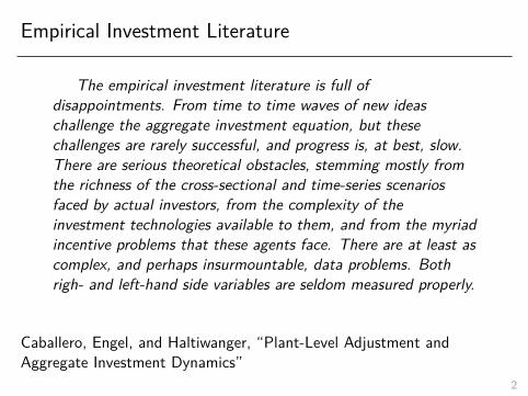
Empirical Investment Literature
The empirical investment literature is full ofdisappointments. From time to time waves of new ideaschallenge the aggregate investment equation, but thesechallenges are rarely successful, and progress is, at best, slow.There are serious theoretical obstacles, stemming mostly fromthe richness of the cross-sectional and time-series scenariosfaced by actual investors, from the complexity of theinvestment technologies available to them, and from the myriadincentive problems that these agents face. There are at least ascomplex, and perhaps insurmountable, data problems. Bothrigh- and left-hand side variables are seldom measured properly.
Caballero, Engel, and Haltiwanger, “Plant-Level Adjustment andAggregate Investment Dynamics”
2

Empirical Investment Literature
• Many early papers focus on neoclassical model
• “User cost” and “q theory” formulations• Finds model does not fit the data well at micro or macro level
• Two main responses:
1. Real adjustment frictions with nonconvexities2. Financial frictions to acquiring investment funds are important
2

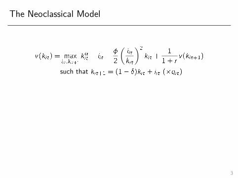
The Neoclassical Model
Consider production side of economy in time t with:
• Firms i 2 [0; 1] with production functionyit = k�it , � � 1
• Invest to accumulate capital kit+1 = (1� �)kit + iit
• Quadratic adjustment costs ��2
(iitkit
)2kit
• Discount future at constant rate r
v(kit) = maxiit ;kit+1
k�it � iit ��
2
(iitkit
)2
kit +1
1 + rv(kit+1)
such that kit+1 = (1� �)kit + iit
3
The Neoclassical Model
v(kit) = maxiit ;kit+1
k�it � iit ��
2
(iitkit
)2
kit +1
1 + rv(kit+1)
such that kit+1 = (1� �)kit + iit (�qit)
Take first order conditions:
1 + �(iitkit
) =qit
qit =v0(kit+1)
=1
1 + r
1∑s=0
(1� �
1 + r
)s (�k��1it+s+1 +�it+s+1
)
3

The Neoclassical Model
v(kit) = maxiit ;kit+1
k�it � iit ��
2
(iitkit
)2
kit +1
1 + rv(kit+1)
such that kit+1 = (1� �)kit + iit (�qit)
Take first order conditions:
1 + �(iitkit
) =qit
qit =v0(kit+1)
=1
1 + r
1∑s=0
(1� �
1 + r
)s (�k��1it+s+1 +�it+s+1
)2

The User Cost Model: � = 0
With � = 0, first order conditions simplify to
qit =1
�k��1it+1︸ ︷︷ ︸MPKit
= r + �︸ ︷︷ ︸user costt
• The user cost of capital is the implicit rental rate on capital
• Typically extended to incorporate other empirically relevant features:
ujt = pt︸︷︷︸relative price
�1�mjt � zjt
1� �t︸ ︷︷ ︸taxes
�(rt + �j)
3

Empirical Performance of the User Cost Model
• Typical regression takes the form
iitkit
= �i + � � uit + �� other variablesit + "it
• Two main failures of user cost model:1. Estimated user cost elasticity � small (� 0 to -0.5)2. Coefficients on other variables, especially cash flow, large and
significant
• Hall and Jorgensen (1967); Cummins, Hassett, and Hubbard (1994);Chirinko, Fazarri, and Meyer (1999)
4

The Q-Theory Model: � � 0
qit =1 + �(iitkit
)
qit =v0(kit+1) =
1
1 + r
1∑s=0
(1� �
1 + r
)s (�k��1it+s+1 +�it+s+1
)
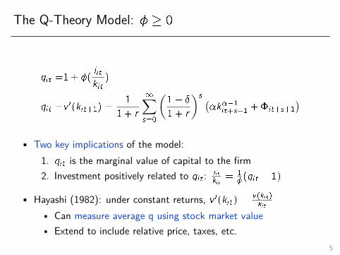
• Two key implications of the model:1. qit is the marginal value of capital to the firm2. Investment positively related to qit : iit
kit= 1
�(qit � 1)
• Hayashi (1982): under constant returns, v 0(kit) = v(kit)kit
• Can measure average q using stock market value• Extend to include relative price, taxes, etc.
5

The Q-Theory Model: � � 0
qit =1 + �(iitkit
)
qit =v0(kit+1) =
1
1 + r
1∑s=0
(1� �
1 + r
)s (�k��1it+s+1 +�it+s+1
)• Two key implications of the model:
1. qit is the marginal value of capital to the firm2. Investment positively related to qit : iit
kit= 1
�(qit � 1)
• Hayashi (1982): under constant returns, v 0(kit) = v(kit)kit
• Can measure average q using stock market value• Extend to include relative price, taxes, etc.
5

Empirical Performance of the Q Model
• Typical regression takes the form
iitkit
= �i + � � qit + �� other variablesit + "it
• Two main failures of user cost model:1. Estimated coefficient � small and unstable2. Coefficients on other variables, especially cash flow, large and
significant
• Summers (1981); Cummins, Hassett, and Hubbard (1994); Ericksonand Whited (2000)
6

Doms and Dunne (1998)
Two responses to failure of neoclassical model:1. Real adjustment frictions featuring nonconvexities are important2. Financial frictions to acquiring investment funds are important
Doms and Dunne (1998):• Landmark descriptive study of investment in LRD
• Shows micro-level investment is lumpy, i.e., occurs mainly alongextensive margin
• Fluctuations in total investment mainly due to extensive margin
• Suggests important role for non-convex adjustment costs
7

Measurement
• Use Census data from LRD, 1972 - 1988• After 1988, stopped collecting book value of capital
• Construct capital stock using perpetual inventory method• Focus on balanced panel
• Analyze the growth rate of capital for plant i at time t
GKit =iit � �kit�1
0:5� (kit�1 + kit)
8

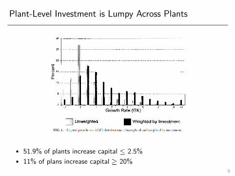
Plant-Level Investment is Lumpy Across Plants
• 51.9% of plants increase capital � 2.5%• 11% of plans increase capital � 20%
9
Plant-Level Investment is Lumpy Across Plants
• 51.9% of plants increase capital � 2.5%• 11% of plans increase capital � 20%
9

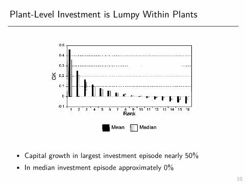
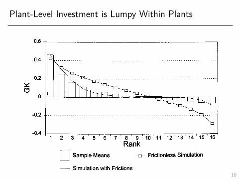
Plant-Level Investment is Lumpy Within Plants
• Capital growth in largest investment episode nearly 50%• In median investment episode approximately 0%
10
Plant-Level Investment is Lumpy Within Plants
• Capital growth in largest investment episode nearly 50%• In median investment episode approximately 0%
10
Plant-Level Investment is Lumpy Within Plants
10
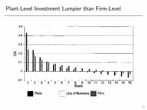
Plant-Level Investment Lumpier than Firm-Level
11

Frequency of Spikes Correlated with AggregateInvestment
12
Zwick and Mahon (2016)
Two responses to failure of neoclassical model:1. Real adjustment frictions featuring nonconvexities are important2. Financial frictions to acquiring investment funds are important
Zwick and Mahon (2016):
• Clean study exploiting exploiting policy-induced variation in cost ofcapital
• Shows investment very responsive to cost, especially forsmall/non-dividend paying firms
• Suggests important role for financial frictions (and potentially fixedcosts)
13

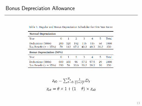
Bonus Depreciation Allowance
• Bonus shifts depreciation allowances from future to present• With discounting, lowers the total cost of investment
! Bonus more valuable for longer-lived investment
14

Bonus Depreciation Allowance
• Bonus shifts depreciation allowances from future to present• With discounting, lowers the total cost of investment
! Bonus more valuable for longer-lived investment14

Bonus Depreciation Allowance
zs0 =∑Ts
t=01
(1+r)tDt
zst = � � 1 + (1� �)� zs0
14
Bonus Depreciation Allowance
zs0 =∑Ts
t=01
(1+r)tDt
zst = � � 1 + (1� �)� zs0
13

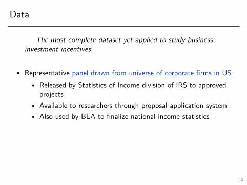
Data
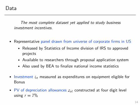
The most complete dataset yet applied to study businessinvestment incentives.
• Representative panel drawn from universe of corporate firms in US• Released by Statistics of Income division of IRS to approved
projects• Available to researchers through proposal application system• Also used by BEA to finalize national income statistics
• Investment iit measured as expenditures on equipment eligible forBonus
• PV of depreciation allowances zst constructed at four digit levelusing r = 7%
14
Data
The most complete dataset yet applied to study businessinvestment incentives.
• Representative panel drawn from universe of corporate firms in US• Released by Statistics of Income division of IRS to approved
projects• Available to researchers through proposal application system• Also used by BEA to finalize national income statistics
• Investment iit measured as expenditures on equipment eligible forBonus
• PV of depreciation allowances zst constructed at four digit levelusing r = 7%
14
Identification Strategy
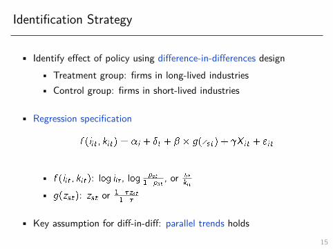
• Identify effect of policy using difference-in-differences design• Treatment group: firms in long-lived industries• Control group: firms in short-lived industries
• Regression specification
f (iit ; kit) = �i + �t + � � g(zst) + Xit + "it
• f (iit ; kit): log iit , log pst
1�pst, or iit
kit
• g(zst): zst or 1��zst1��
• Key assumption for diff-in-diff: parallel trends holds15

Graphical Evidence
16

Overall Effect of Bonus on Investment
f (iit ; kit) = �i + �t + � � g(zst) + Xit + "it17

Larger Effect Than Existing Literature
18

Heterogeneity Suggestive of Financial Frictions
19

Heterogeneity Explains Larger Estimate than Literature
20

Unfair Review of Empirical Investment Lit
• Neoclassical model predicts investment very responsive to cost• User cost formulation: capital stock responds to implied rental
rate• Q theory formulation: investment responds to marginal value of
capital
• 1960s - 1990s: both formulations largely fail in data• Capital/investment unresponsive to cost• Other variables (cash flow) significant
• Two responses to failure of neoclassical model1. Adjustment costs feature nonconvexities2. Financial frictions influence investment behavior
21
The Rest of This Topic
Focus on role of nonconvex adjustment costs in explaining micro andmacro investment dynamics
1. Study models of micro-level investment behavior• What form of adjustment costs do we need to explain micro
data?
2. Study aggregate implications of these models• Aggregation• General equilibrium
22

Plan for this Topic
1. An unfair summary of the empirical investment literature
2. Accounting for micro-level investment behavior with nonconvexadjustment costs
3. Macro implications of nonconvex adjustment costs
22
The Gold Standard: Cooper and Haltiwanger (2006)
• What types of adjustment costs do we need to match micro-levelinvestment behavior?
• Pays special attention to lumpy nature of investment
• Answer using an estimated structural model• Simulated method of moments
• A note on terminology in this literature:• Partial equilibrium = analyzing decision rules with fixed prices• Does NOT mean equilibrium in one market! (which would be
correct)
23
The Gold Standard: Cooper and Haltiwanger (2006)
• What types of adjustment costs do we need to match micro-levelinvestment behavior?
• Pays special attention to lumpy nature of investment
• Answer using an estimated structural model• Simulated method of moments
• A note on terminology in this literature:• Partial equilibrium = analyzing decision rules with fixed prices• Does NOT mean equilibrium in one market!
(which would becorrect)
23
The Gold Standard: Cooper and Haltiwanger (2006)
• What types of adjustment costs do we need to match micro-levelinvestment behavior?
• Pays special attention to lumpy nature of investment
• Answer using an estimated structural model• Simulated method of moments
• A note on terminology in this literature:• Partial equilibrium = analyzing decision rules with fixed prices• Does NOT mean equilibrium in one market! (which would be
correct)23
LRD Data
Sample• Establishment-level observations• Balanced panel: model abstracts from entry and exit• 1972 - 1988: want to use data on expenditures and retirements
Measurement• Investment iit : expenditureit � retirmentsit• Capital kit : kit+1 = (1� �it)kit + iit
• Depreciation �it : constructed to reflect in-use depreciation
24

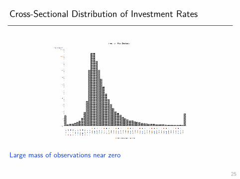
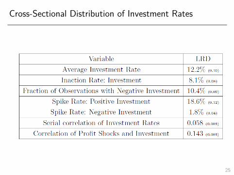
Cross-Sectional Distribution of Investment Rates
Large mass of observations near zeroHighly skewed and fat right tails
25
Cross-Sectional Distribution of Investment Rates
Large mass of observations near zero
Highly skewed and fat right tails
25

Cross-Sectional Distribution of Investment Rates
Large mass of observations near zeroHighly skewed and fat right tails
25
Cross-Sectional Distribution of Investment Rates
25

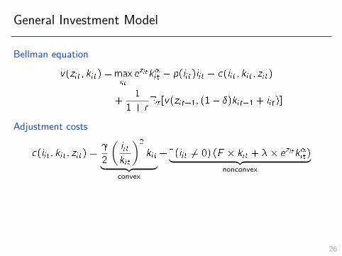
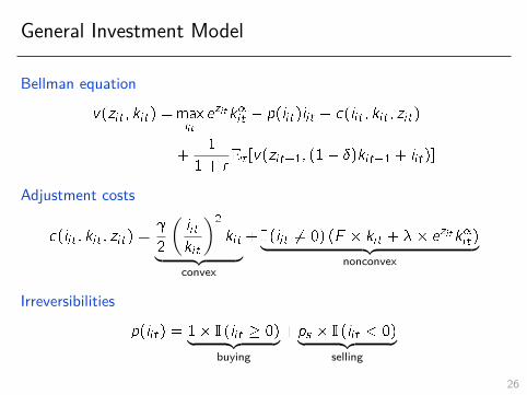
General Investment Model
Bellman equation
v(zit ; kit) =maxiitezitk�it � p(iit)iit � c(iit ; kit ; zit)
+1
1 + rEt [v(zit+1; (1� �)kit+1 + iit)]
Adjustment costs
c(iit ; kit ; zit) =
2
(iitkit
)2
kit︸ ︷︷ ︸convex
+ I (iit 6= 0) (F � kit + �� ezitk�it )︸ ︷︷ ︸
nonconvex
Irreversibilities
p(iit) = 1� I (iit � 0)︸ ︷︷ ︸buying
+ ps � I (iit < 0)︸ ︷︷ ︸selling
26

No Adjustment Costs
v(zit ; kit) =maxiitezitk�it � iit +
1
1 + rEt [v(zit+1; (1� �)kit+1 + iit)]
Optimal Behavior
1 =1
1 + rEt [v2(zit+1; kit+1)]
! user cost model: r + � = Et [�k��1it+1]
27

No Adjustment Costs
v(zit ; kit) =maxiitezitk�it � iit +
1
1 + rEt [v(zit+1; (1� �)kit+1 + iit)]
Optimal Behavior
1 =1
1 + rEt [v2(zit+1; kit+1)]
! user cost model: r + � = Et [�k��1it+1]
27

Convex Costs Only
v(zit ; kit) =maxiitezitk�it � iit � c(iit ; kit ; zit) +
1
1 + rEt [v(zit+1; kit+1)]
c(iit ; kit ; zit) =
2
(iitkit
)2
kit
Optimal Behavior
1 +
(iitkit
)=
1
1 + rEt [v2(zit+1; kit+1)]
! q model: iitkit
=1
(Et [v2(zit+1; kit+1)]� 1)
28

Convex Costs Only
v(zit ; kit) =maxiitezitk�it � iit � c(iit ; kit ; zit) +
1
1 + rEt [v(zit+1; kit+1)]
c(iit ; kit ; zit) =
2
(iitkit
)2
kit
Optimal Behavior
1 +
(iitkit
)=
1
1 + rEt [v2(zit+1; kit+1)]
! q model: iitkit
=1
(Et [v2(zit+1; kit+1)]� 1)
28

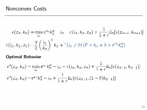
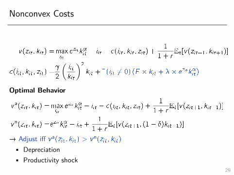
Nonconvex Costs
v(zit ; kit) =maxiitezitk�it � iit � c(iit ; kit ; zit) +
1
1 + rEt [v(zit+1; kit+1)]
c(iit ; kit ; zit) =
2
(iitkit
)2
kit + I (iit 6= 0) (F � kit + �� ezitk�it )
Optimal Behavior
v a(zit ; kit) =maxiitezitk�it � iit � c(iit ; kit ; zit) +
1
1 + rEt [v(zit+1; kit+1)]
vn(zit ; kit) =ezitk�it � iit +
1
1 + rEt [v(zit+1; (1� �)kit+1)]
! Adjust iff v a(zit ; kit) > vn(zit ; kit)
• Depreciation• Productivity shock
29
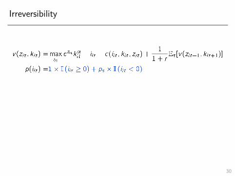
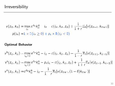
Irreversibility
v(zit ; kit) =maxiitezitk�it � iit � c(iit ; kit ; zit) +
1
1 + rEt [v(zit+1; kit+1)]
p(iit) =1� I (iit � 0) + ps � I (iit < 0)
Optimal Behavior
vb(zit ; kit) =maxiit�0
ezitk�it � iit � c(iit ; kit ; zit) +1
1 + rEt [v(zit+1; kit+1)]
v s(zit ; kit) =maxiit<0
ezitk�it � ps iit � c(iit ; kit ; zit) +1
1 + rEt [v(zit+1; kit+1)]
vn(zit ; kit) =ezitk�it � iit +
1
1 + rEt [v(zit+1; (1� �)kit+1)]
! Also generates inaction
30

Irreversibility
v(zit ; kit) =maxiitezitk�it � iit � c(iit ; kit ; zit) +
1
1 + rEt [v(zit+1; kit+1)]
p(iit) =1� I (iit � 0) + ps � I (iit < 0)
Optimal Behavior
vb(zit ; kit) =maxiit�0
ezitk�it � iit � c(iit ; kit ; zit) +1
1 + rEt [v(zit+1; kit+1)]
v s(zit ; kit) =maxiit<0
ezitk�it � ps iit � c(iit ; kit ; zit) +1
1 + rEt [v(zit+1; kit+1)]
vn(zit ; kit) =ezitk�it � iit +
1
1 + rEt [v(zit+1; (1� �)kit+1)]
! Also generates inaction30

Illustration of Various Frictions
31
Model Quantification
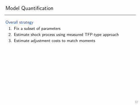
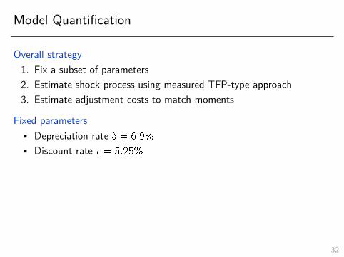
Overall strategy1. Fix a subset of parameters2. Estimate shock process using measured TFP-type approach3. Estimate adjustment costs to match moments
Fixed parameters• Depreciation rate � = 6:9%
• Discount rate r = 5:25%
Estimate idiosyncratic shocks• Assume zit = "it + bt
• Assume AR(1) and use GMM onlog(�it) = �� log(�it�1) + �kit � ���kit�1 + bt � ��bt�1 + �it
• See paper for details
32
Model Quantification
Overall strategy1. Fix a subset of parameters2. Estimate shock process using measured TFP-type approach3. Estimate adjustment costs to match moments
Fixed parameters• Depreciation rate � = 6:9%
• Discount rate r = 5:25%
Estimate idiosyncratic shocks• Assume zit = "it + bt
• Assume AR(1) and use GMM onlog(�it) = �� log(�it�1) + �kit � ���kit�1 + bt � ��bt�1 + �it
• See paper for details
32

Model Quantification
Overall strategy1. Fix a subset of parameters2. Estimate shock process using measured TFP-type approach3. Estimate adjustment costs to match moments
Fixed parameters• Depreciation rate � = 6:9%
• Discount rate r = 5:25%
Estimate idiosyncratic shocks• Assume zit = "it + bt
• Assume AR(1) and use GMM onlog(�it) = �� log(�it�1) + �kit � ���kit�1 + bt � ��bt�1 + �it
• See paper for details32
Estimating Adjustment Cost Parameters
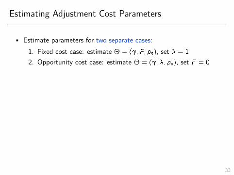
• Estimate parameters for two separate cases:1. Fixed cost case: estimate � = ( ; F; ps), set � = 1
2. Opportunity cost case: estimate � = ( ; �; ps), set F = 0
• Simulated Method of Moments (SMM)
�̂ = argmin�
[d �s(�)]T W [d �s(�)]
• Data moments d: drawn from data• Model moments s(�): simulated panel of firms from model• Weighting matrix W : efficient matrix from GMM• Standard errors: GMM formulas plus factor for Monte Carlo
error
33

Estimating Adjustment Cost Parameters
• Estimate parameters for two separate cases:1. Fixed cost case: estimate � = ( ; F; ps), set � = 1
2. Opportunity cost case: estimate � = ( ; �; ps), set F = 0
• Simulated Method of Moments (SMM)
�̂ = argmin�
[d �s(�)]T W [d �s(�)]
• Data moments d: drawn from data• Model moments s(�): simulated panel of firms from model• Weighting matrix W : efficient matrix from GMM• Standard errors: GMM formulas plus factor for Monte Carlo
error33

Estimation Results: Fixed Cost Case
Estimated fixed cost F u 4% of capital stock
34

Estimation Results: Fixed Cost Case
Estimated fixed cost F u 4% of capital stock
34
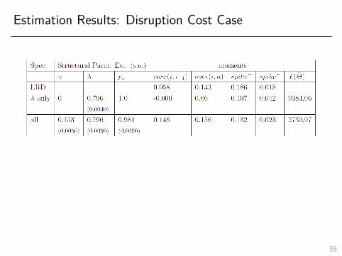
Estimation Results: Disruption Cost Case
Estimated disruption cost 1� � u 20% of profitsOn average, pay 3.1% of profits in AC when adjust
35

Estimation Results: Disruption Cost Case
Estimated disruption cost 1� � u 20% of profitsOn average, pay 3.1% of profits in AC when adjust
35
Cooper and Haltiwanger (2006): Wrapping Up
• What types of adjustment costs do we need to match micro data?
Non-convexities:• Fixed costs• Disruption costs• Irreversibilities
• Nice illustration of Simulated Method of Moments (SMM)methodology
• Specify moments of the data you think are important• Select parameters which are well-identified by those moments• Choose parameters to get model as close as possible to data
• My HW2 will give you practice in simple investment problem
36

Cooper and Haltiwanger (2006): Wrapping Up
• What types of adjustment costs do we need to match micro data?Non-convexities:
• Fixed costs• Disruption costs• Irreversibilities
• Nice illustration of Simulated Method of Moments (SMM)methodology
• Specify moments of the data you think are important• Select parameters which are well-identified by those moments• Choose parameters to get model as close as possible to data
• My HW2 will give you practice in simple investment problem36

Asker, Collard-Wexler, and De Loecker (2014)
Shows Cooper-Haltiwanger (2006) model also explains much of MRPKit
dispersion documented by Hsieh and Klenow (2009)
Data: LRD, 1972 - 1997• Also use cross-country data for analysis in paper
Model: Cooper-Haltiwanger (2006) opportunity cost model
v(zit ; kit) =maxiitezitk�it � iit � c(iit ; kit ; zit) +
1
1 + rEt [v(zit+1; kit+1)]
c(iit ; kit ; zit) =
2
(iitkit
)2
kit + I (iit 6= 0)�� ezitk�it
37

Estimation
Estimate � = ( ; �) using SMM
�̂ = argmin�
[d �s(�)]T W [d �s(�)]
38

Estimation
Estimate � = ( ; �) using SMM
�̂ = argmin�
[d �s(�)]T W [d �s(�)]
38
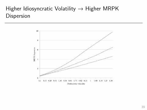
Higher Idiosyncratic Volatility ! Higher MRPKDispersion
• MRPKit = � yitkit
• Time to build ! ex-ante dispersion• Adjustment costs ! ex-post dispersion
39

Higher Idiosyncratic Volatility ! Higher MRPKDispersion
• MRPKit = � yitkit
• Time to build ! ex-ante dispersion• Adjustment costs ! ex-post dispersion 39

Idiosyncratic Volatility and MRPK Dispersion in Data
40

Idiosyncratic Volatility and MRPK Dispersion in Data
40
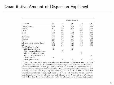
Quantitative Amount of Dispersion Explained
41

Plan for this Topic
1. An unfair summary of the empirical investment literature
2. Accounting for micro-level investment behavior with nonconvexadjustment costs
3. Macro implications of nonconvex adjustment costs
41

Aggregate Implications of Micro Investment Models
1. Aggregation of micro-level models holding prices fixed (partialequilibrium)
• Response of aggregate investment to shocks depends onnumber of firms who adjust
• Aggregate investment features time-varying elasticity w.r.t.shocks
• Representative firm instead predicts constant elasticity
2. Endogenize prices in general equilibrium• In benchmark RBC framework, procyclical real interest rate
eliminates time-varying elasticity• Modifications to benchmark model can break this irrelevance
result
42

Aggregate Implications of Micro Investment Models
1. Aggregation of micro-level models holding prices fixed (partialequilibrium)
• Response of aggregate investment to shocks depends onnumber of firms who adjust
• Aggregate investment features time-varying elasticity w.r.t.shocks
• Representative firm instead predicts constant elasticity
2. Endogenize prices in general equilibrium• In benchmark RBC framework, procyclical real interest rate
eliminates time-varying elasticity• Modifications to benchmark model can break this irrelevance
result42

General Lessons
1. Anytime you go from micro to macro, need to think about• Aggregation• General equilibrium
2. Macro models with micro heterogeneity are hard• Entire cross-sectional distribution of agents part of state vector• Difficult to numerically compute and estimate
• Aggregate implications of lumpy investment models good illustrationof these more general issues
• Each of these steps has been extensively studied• But people are largely tired of it by now
43

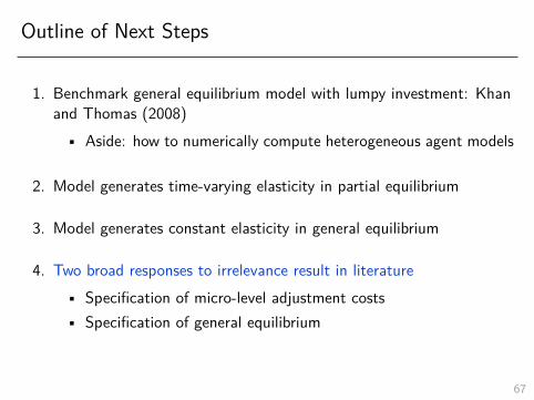
Outline of Next Steps
1. Benchmark general equilibrium model with lumpy investment: Khanand Thomas (2008)
• Aside: how to numerically compute heterogeneous agent models
2. Model generates time-varying elasticity in partial equilibrium
3. Model generates constant elasticity in general equilibrium
4. Two broad responses to irrelevance result in literature• Specification of micro-level adjustment costs• Specification of general equilibrium
44
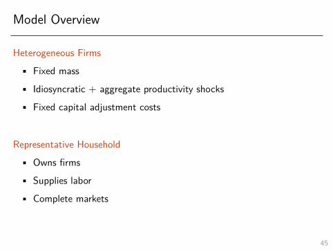
Model Overview
Heterogeneous Firms• Fixed mass• Idiosyncratic + aggregate productivity shocks• Fixed capital adjustment costs
Representative Household• Owns firms• Supplies labor• Complete markets
45
Firms
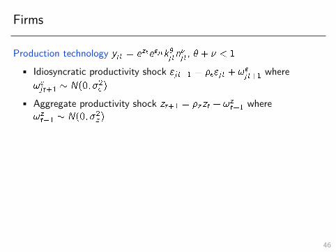
Production technology yjt = ezte"jtk�jtn�jt , � + � < 1
• Idiosyncratic productivity shock "jt+1 = ��"jt + !"jt+1 where
!"jt+1 � N(0; �2� )
• Aggregate productivity shock zt+1 = �zzt + !zt+1 where
!zt+1 � N(0; �2z )
Firms accumulate capital according to kjt+1 = (1� �)kjt + ijt
• If ijtkjt=2 [�a; a], pay fixed cost �jt in units of labor
• Fixed cost �jt � U[0; �]
46

Firms
Production technology yjt = ezte"jtk�jtn�jt , � + � < 1
• Idiosyncratic productivity shock "jt+1 = ��"jt + !"jt+1 where
!"jt+1 � N(0; �2� )
• Aggregate productivity shock zt+1 = �zzt + !zt+1 where
!zt+1 � N(0; �2z )
Firms accumulate capital according to kjt+1 = (1� �)kjt + ijt
• If ijtkjt=2 [�a; a], pay fixed cost �jt in units of labor
• Fixed cost �jt � U[0; �]
46

Firm Optimization Problem: Recursive Formulation
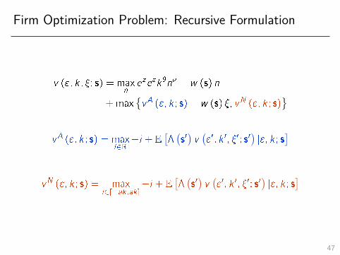
v ("; k; �; s) = maxneze"k�n� � w (s) n
+max{vA ("; k ; s)� w (s) �; vN ("; k ; s)
}
47
Firm Optimization Problem: Recursive Formulation
v ("; k; �; s) = maxneze"k�n� � w (s) n
+max{vA ("; k ; s)� w (s) �; vN ("; k ; s)
}vA ("; k ; s) = max
i2R�i + E
[�(s0)v("0; k 0; �0; s0
)j"; k ; s
]
vN ("; k ; s) = maxi2[�ak;ak]
�i + E[�(s0)v("0; k 0; �0; s0
)j"; k ; s
]
47

Firm Optimization Problem: Recursive Formulation
v ("; k; �; s) = maxneze"k�n� � w (s) n
+max{vA ("; k ; s)� w (s) �; vN ("; k ; s)
}
v̂ ("; k ; s) = maxneze"k�n� � w (s) n
+�̂ ("; k ; s)
�
(vA ("; k ; s)� w (s)
�̂ ("; k ; s)
2
)
+
(1�
�̂ ("; k ; s)
�
)vN ("; k ; s)
47
Household
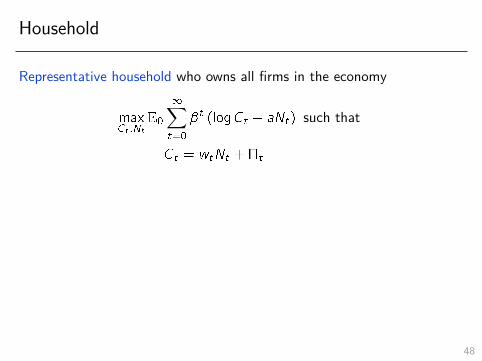
Representative household who owns all firms in the economy
maxCt ;Nt
E0
1∑t=0
�t (logCt � aNt) such that
Ct = wtNt +�t
Complete markets implies that �t;t+1 = �(Ct+1
Ct
)�1• Firms maximize their market value• Market value given by expected present value of dividends using
stochastic discount factor• With complete markets, SDF is household’s marginal rate of
substitution
48

Household
Representative household who owns all firms in the economy
maxCt ;Nt
E0
1∑t=0
�t (logCt � aNt) such that
Ct = wtNt +�t
Complete markets implies that �t;t+1 = �(Ct+1
Ct
)�1• Firms maximize their market value• Market value given by expected present value of dividends using
stochastic discount factor• With complete markets, SDF is household’s marginal rate of
substitution48

Defining Recursive Competitive Equilibrium
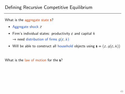
What is the aggregate state s?
• Aggregate shock z• Firm’s individual states: productivity " and capital k! need distribution of firms g("; k)
• Will be able to construct all household objects using s = (z; g("; k))
What is the law of motion for the s?
gt+1("0; k 0
)=
∫ [1 f�""+ �"!
0" = "0g
�∫1 fk 0t ("; k; �) = k 0g dG(�)
]� p
(!0")gt ("; k) d!
0"d"dk
49

Defining Recursive Competitive Equilibrium
What is the aggregate state s?• Aggregate shock z
• Firm’s individual states: productivity " and capital k! need distribution of firms g("; k)
• Will be able to construct all household objects using s = (z; g("; k))
What is the law of motion for the s?
gt+1("0; k 0
)=
∫ [1 f�""+ �"!
0" = "0g
�∫1 fk 0t ("; k; �) = k 0g dG(�)
]� p
(!0")gt ("; k) d!
0"d"dk
49

Defining Recursive Competitive Equilibrium
What is the aggregate state s?• Aggregate shock z• Firm’s individual states: productivity " and capital k
! need distribution of firms g("; k)• Will be able to construct all household objects using s = (z; g("; k))
What is the law of motion for the s?
gt+1("0; k 0
)=
∫ [1 f�""+ �"!
0" = "0g
�∫1 fk 0t ("; k; �) = k 0g dG(�)
]� p
(!0")gt ("; k) d!
0"d"dk
49

Defining Recursive Competitive Equilibrium
What is the aggregate state s?• Aggregate shock z• Firm’s individual states: productivity " and capital k! need distribution of firms g("; k)
• Will be able to construct all household objects using s = (z; g("; k))
What is the law of motion for the s?
gt+1("0; k 0
)=
∫ [1 f�""+ �"!
0" = "0g
�∫1 fk 0t ("; k; �) = k 0g dG(�)
]� p
(!0")gt ("; k) d!
0"d"dk
49

Defining Recursive Competitive Equilibrium
What is the aggregate state s?• Aggregate shock z• Firm’s individual states: productivity " and capital k! need distribution of firms g("; k)
• Will be able to construct all household objects using s = (z; g("; k))
What is the law of motion for the s?
gt+1("0; k 0
)=
∫ [1 f�""+ �"!
0" = "0g
�∫1 fk 0t ("; k; �) = k 0g dG(�)
]� p
(!0")gt ("; k) d!
0"d"dk
49

Recursive Competitive Equilibrium
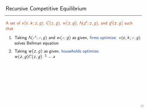
A set of v("; k ; z; g), C(z; g), w(z; g), �(z 0; z; g), and g0(z; g) suchthat
1. Taking �(z 0; z; g) and w(z; g) as given, firms optimize: v("; k ; z; g)solves Bellman equation
2. Taking w(z; g) as given, households optimize:w(z; g)C(z; g)�1 = a
3. Markets clear and aggregate consistency conditions hold:
�(z 0; z; g) = �
(C(z 0; g0(z; g))
C(z; g)
)�1C(z; g) =
∫(y("; k; �; z; g)� i("; k; �; z; g))dG(�)g("; k)d"dk
g0("; k) satisfies law of motion for distribution
50

Recursive Competitive Equilibrium
A set of v("; k ; z; g), C(z; g), w(z; g), �(z 0; z; g), and g0(z; g) suchthat
1. Taking �(z 0; z; g) and w(z; g) as given, firms optimize: v("; k ; z; g)solves Bellman equation
2. Taking w(z; g) as given, households optimize:w(z; g)C(z; g)�1 = a
3. Markets clear and aggregate consistency conditions hold:
�(z 0; z; g) = �
(C(z 0; g0(z; g))
C(z; g)
)�1C(z; g) =
∫(y("; k; �; z; g)� i("; k; �; z; g))dG(�)g("; k)d"dk
g0("; k) satisfies law of motion for distribution
50
Outline of Next Steps
1. Benchmark general equilibrium model with lumpy investment: Khanand Thomas (2008)
• Aside: how to numerically compute heterogeneous agent models
2. Model generates time-varying elasticity in partial equilibrium
3. Model generates constant elasticity in general equilibrium
4. Two broad responses to irrelevance result in literature• Specification of micro-level adjustment costs• Specification of general equilibrium
50

Computing Equilibrium
• Key challenge: aggregate state g is infinite-dimensional
• Two steps:1. Compute steady state without aggregate shocks ! distribution
constant at g�
2. Compute full model with aggregate shocks ! distributionvaries over time
• Today will give you an overview to help you read papers• My HW2: solve steady state• With Greg: compute aggregate dynamics
51

Steady State Recursive Competitive Equilibrium
A set of v�("; k), C�, w�, and g�("; k) such that
1. Taking w� as given, firms optimize: v�("; k) solves Bellmanequation
2. Taking w� as given, households optimize: w�(C�)�1 = a
3. Markets clear and aggregate consistency conditions hold:
C� =
∫(y("; k; �)� i("; k; �))dG(�)g�("; k)d"dk
g�("; k) satisfies law of motion for distribution given g�
52

Hopenhayn-Rogerson (1993) Algorithm
Start with guess of w�
• Solve firm optimization problem ! v�("; k)
• Compute stationary distribution g�("; k)
• Compute implied aggregate consumption C�
• Check household optimization w�(C�)�1 = a
Update guess of w�
53

Hopenhayn-Rogerson (1993) Algorithm
Start with guess of w�
• Solve firm optimization problem ! v�("; k)
• Compute stationary distribution g�("; k)
• Compute implied aggregate consumption C�
• Check household optimization w�(C�)�1 = a
Update guess of w�
53
Hopenhayn-Rogerson (1993) Algorithm
Start with guess of w�
• Solve firm optimization problem ! v�("; k)
• Compute stationary distribution g�("; k)
• Compute implied aggregate consumption C�
• Check household optimization w�(C�)�1 = a
Update guess of w�
53

Hopenhayn-Rogerson (1993) Algorithm
Start with guess of w�
• Solve firm optimization problem ! v�("; k)
• Compute stationary distribution g�("; k)
• Compute implied aggregate consumption C�
• Check household optimization w�(C�)�1 = a
Update guess of w�
53

Hopenhayn-Rogerson (1993) Algorithm
Start with guess of w�
• Solve firm optimization problem ! v�("; k)
• Compute stationary distribution g�("; k)
• Compute implied aggregate consumption C�
• Check household optimization w�(C�)�1 = a
Update guess of w�
53

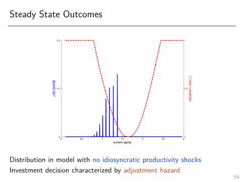
Steady State Outcomes
Distribution in model with no idiosyncratic productivity shocksInvestment decision characterized by adjustment hazard
54

Steady State Outcomes
Distribution in model with no idiosyncratic productivity shocks
Investment decision characterized by adjustment hazard
54
Steady State Outcomes
Distribution in model with no idiosyncratic productivity shocksInvestment decision characterized by adjustment hazard
54
Full Model with Aggregate Shocks
• Outside of steady state, three key challenges
1. Distribution g varies over time ! how to approximatedistribution?
2. Law of motion for g is complicated ! how to approximate lawof motion?
3. Prices are functions of distribution ! how to approximate thesefunctions?
• Will briefly describe two approaches to dealing with these challenges1. Krusell and Smith (1998): approximate distribution with
moments2. Winberry (2016): approximate distribution with flexible
parametric family
• Next quarter you will learn how continuous time makes this easier(Ahn-Kaplan-Moll-Winberry-Wolf)
55

Full Model with Aggregate Shocks
• Outside of steady state, three key challenges1. Distribution g varies over time ! how to approximate
distribution?
2. Law of motion for g is complicated ! how to approximate lawof motion?
3. Prices are functions of distribution ! how to approximate thesefunctions?
• Will briefly describe two approaches to dealing with these challenges1. Krusell and Smith (1998): approximate distribution with
moments2. Winberry (2016): approximate distribution with flexible
parametric family
• Next quarter you will learn how continuous time makes this easier(Ahn-Kaplan-Moll-Winberry-Wolf)
55

Full Model with Aggregate Shocks
• Outside of steady state, three key challenges1. Distribution g varies over time ! how to approximate
distribution?2. Law of motion for g is complicated ! how to approximate law
of motion?
3. Prices are functions of distribution ! how to approximate thesefunctions?
• Will briefly describe two approaches to dealing with these challenges1. Krusell and Smith (1998): approximate distribution with
moments2. Winberry (2016): approximate distribution with flexible
parametric family
• Next quarter you will learn how continuous time makes this easier(Ahn-Kaplan-Moll-Winberry-Wolf)
55
Full Model with Aggregate Shocks
• Outside of steady state, three key challenges1. Distribution g varies over time ! how to approximate
distribution?2. Law of motion for g is complicated ! how to approximate law
of motion?3. Prices are functions of distribution ! how to approximate these
functions?
• Will briefly describe two approaches to dealing with these challenges1. Krusell and Smith (1998): approximate distribution with
moments2. Winberry (2016): approximate distribution with flexible
parametric family
• Next quarter you will learn how continuous time makes this easier(Ahn-Kaplan-Moll-Winberry-Wolf)
55
Full Model with Aggregate Shocks
• Outside of steady state, three key challenges1. Distribution g varies over time ! how to approximate
distribution?2. Law of motion for g is complicated ! how to approximate law
of motion?3. Prices are functions of distribution ! how to approximate these
functions?
• Will briefly describe two approaches to dealing with these challenges1. Krusell and Smith (1998): approximate distribution with
moments2. Winberry (2016): approximate distribution with flexible
parametric family
• Next quarter you will learn how continuous time makes this easier(Ahn-Kaplan-Moll-Winberry-Wolf) 55
Krusell and Smith (1998)
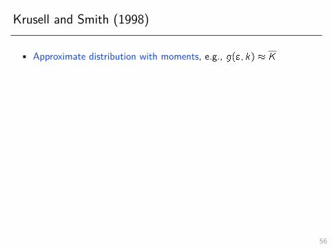
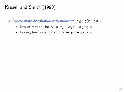
• Approximate distribution with moments, e.g., g("; k) � K
• Law of motion: logK0= �0 + �1z + �2 logK
• Pricing functions: logC = 0 + 1z + 2 logK
• Given guess � and
• Compute individual decisions v("; k ; z;K)• Simulate decision rules ! fKt ; Ct ; ztg
• Update � and using OLS
• R2 on regressions typical accuracy measure• Problems with this measure: Den Haan (2010)• Only K matters ! distribution not important (“approximate
aggregation”)
56

Krusell and Smith (1998)
• Approximate distribution with moments, e.g., g("; k) � K
• Law of motion: logK0= �0 + �1z + �2 logK
• Pricing functions: logC = 0 + 1z + 2 logK
• Given guess � and
• Compute individual decisions v("; k ; z;K)• Simulate decision rules ! fKt ; Ct ; ztg
• Update � and using OLS
• R2 on regressions typical accuracy measure• Problems with this measure: Den Haan (2010)• Only K matters ! distribution not important (“approximate
aggregation”)
56

Krusell and Smith (1998)
• Approximate distribution with moments, e.g., g("; k) � K
• Law of motion: logK0= �0 + �1z + �2 logK
• Pricing functions: logC = 0 + 1z + 2 logK
• Given guess � and
• Compute individual decisions v("; k ; z;K)• Simulate decision rules ! fKt ; Ct ; ztg
• Update � and using OLS
• R2 on regressions typical accuracy measure• Problems with this measure: Den Haan (2010)• Only K matters ! distribution not important (“approximate
aggregation”)56

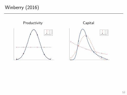
Winberry (2016)
• Approximate distribution with parametric family:
g ("; k) �= g0 expfg11
("�m1
1
)+ g21
(k �m2
1
)+
ng∑i=2
i∑j=0
gji
[("�m1
1
)i�j (k �m2
1
)j�mj
i
]g
! Aggregate state approximated by (z; g("; k)) � (z;m)
• Compute law of motion + prices directly by integration
• Compute aggregate dynamics using perturbation methods• Solve for steady state in Matlab• Solve for aggregate dynamics using Dynare
57
Winberry (2016)
Productivity Capitalng = 1
ng = 2
ng = 6
Exact
ng = 1
ng = 2
ng = 6
Exact
• Run time � 20 - 40 seconds for accurate approximation• Fast enough for likelihood-based estimation• Codes at my website
58

Winberry (2016)
Productivity Capitalng = 1
ng = 2
ng = 6
Exact
ng = 1
ng = 2
ng = 6
Exact
• Run time � 20 - 40 seconds for accurate approximation• Fast enough for likelihood-based estimation• Codes at my website
58
Outline of Next Steps
1. Benchmark general equilibrium model with lumpy investment: Khanand Thomas (2008)
• Aside: how to numerically compute heterogeneous agent models
2. Model generates time-varying elasticity in partial equilibrium
3. Model generates constant elasticity in general equilibrium
4. Two broad responses to irrelevance result in literature• Specification of micro-level adjustment costs• Specification of general equilibrium
58

Khan and Thomas (2008) Calibration
Parameter Description ValueHouseholds� Discount factor :961
Labor disutility N� = 13
Firms� Labor share :64
� Capital share :256
� Capital depreciation :085
� Fixed cost :0083
a No fixed cost region :011
�" Idiosyncratic TFP AR(1) :859
�" Idiosyncratic TFP AR(1) :022
Aggregate shock�z Aggregate TFP AR(1) :859
�z Aggregate TFP AR(1) :014
59
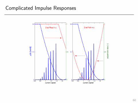
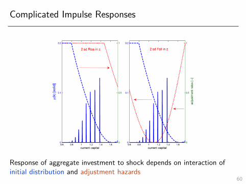
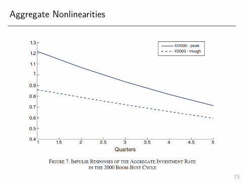
Complicated Impulse Responses
Response of aggregate investment to shock depends on interaction ofinitial distribution and adjustment hazards
60
Complicated Impulse Responses
Response of aggregate investment to shock depends on interaction ofinitial distribution and adjustment hazards
60

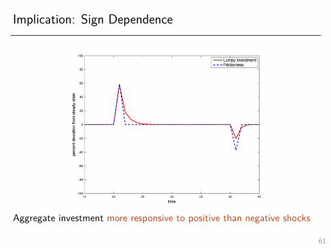
Implication: Sign Dependence
Aggregate investment more responsive to positive than negative shocksNote true in frictionless model
61
Implication: Sign Dependence
Aggregate investment more responsive to positive than negative shocks
Note true in frictionless model
61

Implication: Sign Dependence
Aggregate investment more responsive to positive than negative shocksNote true in frictionless model
61
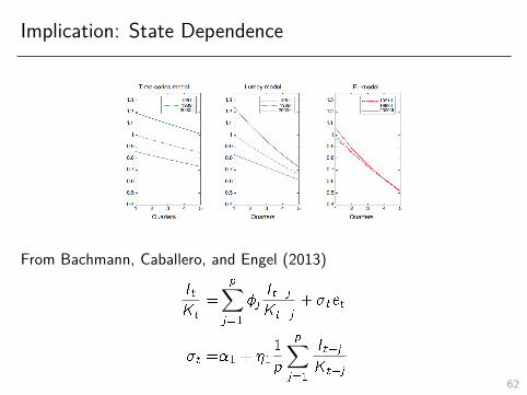
Implication: State Dependence
From Bachmann, Caballero, and Engel (2013)
It
Kt
=
p∑j=1
�jIt�jKt�j
+ �tet
�t =�1 + �11
p
p∑j=1
It�jKt�j
62

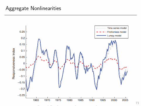
Aggregate Nonlinearities
• Both of these are examples of nonlinear aggregate dynamics• Linear model has constant loading on aggregate shock
• Some evidence in aggregate data• Sign and state dependence ! distribution of It
Ktpositively
skewed• State dependence ! dynamics of It
Ktfeature conditional
heteroskedasticity
• My view: time series evidence is suggestive at best• Predictions are about extreme states, which are rare• But that is exactly when we care about these predictions!! rely on cross-sectional data + carefully specified generalequilibrium model
63
Outline of Next Steps
1. Benchmark general equilibrium model with lumpy investment: Khanand Thomas (2008)
• Aside: how to numerically compute heterogeneous agent models
2. Model generates time-varying elasticity in partial equilibrium
3. Model generates constant elasticity in general equilibrium
4. Two broad responses to irrelevance result in literature• Specification of micro-level adjustment costs• Specification of general equilibrium
5. If time, discuss policy implications63

Distribution of Aggregate It
Kt
in Partial Equilibrium
64

Distribution of Aggregate It
Kt
in General Equilibrium
65

Distribution of Aggregate It
Kt
in General Equilibrium
65
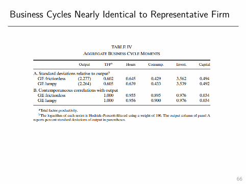
Business Cycles Nearly Identical to Representative Firm
66
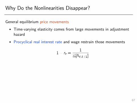
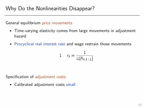
Why Do the Nonlinearities Disappear?
General equilibrium price movements• Time-varying elasticity comes from large movements in adjustment
hazard• Procyclical real interest rate and wage restrain those movements
1 + rt =1
E[�t;t+1]
Specification of adjustment costs• Calibrated adjustment costs small
67
Outline of Next Steps
1. Benchmark general equilibrium model with lumpy investment: Khanand Thomas (2008)
• Aside: how to numerically compute heterogeneous agent models
2. Model generates time-varying elasticity in partial equilibrium
3. Model generates constant elasticity in general equilibrium
4. Two broad responses to irrelevance result in literature• Specification of micro-level adjustment costs• Specification of general equilibrium
67

Outline of Next Steps
1. Benchmark general equilibrium model with lumpy investment: Khanand Thomas (2008)
• Aside: how to numerically compute heterogeneous agent models
2. Model generates time-varying elasticity in partial equilibrium
3. Model generates constant elasticity in general equilibrium
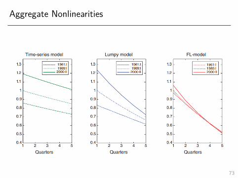
4. Two broad responses to irrelevance result in literature• Specification of micro-level adjustment costs: Bachmann,
Caballero, Engel (2013), Gourio and Kashyap (2007)• Specification of general equilibrium
67

Bachmann, Caballero, and Engel (2013)
• Argue Khan and Thomas’ calibration of adjustment costsresponsible for irrelevance result
• Calibrate larger adjustment costs and recover aggregatenonlinearities
• Argument based on decomposition between AC smoothing and PRsmoothing
• Frictionless partial equilibrium model excessively volatile• AC smoothing: dampening due to adjustment costs• PR smoothing: dampening due to price movements
• Measure AC smoothing in data and target in calibration ! higheradjustment costs
68
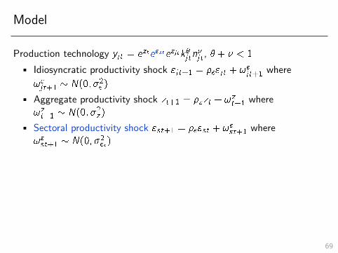
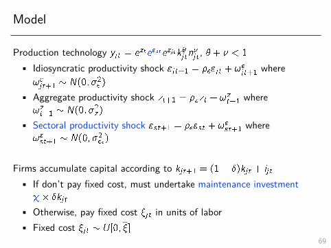
Model
Production technology yjt = ezte"ste"jtk�jtn�jt , � + � < 1
• Idiosyncratic productivity shock "jt+1 = ��"jt + !"jt+1 where
!"jt+1 � N(0; �2� )
• Aggregate productivity shock zt+1 = �zzt + !zt+1 where
!zt+1 � N(0; �2z )
• Sectoral productivity shock "st+1 = ��"st + !"st+1 where
!"st+1 � N(0; �2�s )
Firms accumulate capital according to kjt+1 = (1� �)kjt + ijt
• If don’t pay fixed cost, must undertake maintenance investment�� �kjt
• Otherwise, pay fixed cost �jt in units of labor• Fixed cost �jt � U[0; �]
69

Calibration
Set most parameters exogenously
Choose �z , �, and � to match degree of AC-smoothing• Identify AC-smoothing using volatility of sectoral investment rates
• Aggregated enough to capture interaction of distribution andhazards
• Small enough to not generate price response
• Targets:1. Volatility of aggregate investment rate2. Average volatility of sectoral investment rates3. Amount of conditional heteroskedasticity
70

AC vs. PR Smoothing Decomposition
UB = log [�(none)=�(AC)] = log [�(none)=�(both)]LB =1� log [�(none)=�(PR)] = log [�(none)=�(both)]
71
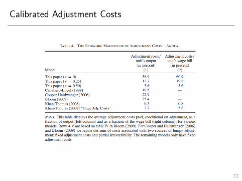
Calibrated Adjustment Costs
72

Aggregate Nonlinearities
73
Aggregate Nonlinearities
73
Aggregate Nonlinearities
73
Aggregate Nonlinearities
73
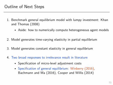
Outline of Next Steps
1. Benchmark general equilibrium model with lumpy investment: Khanand Thomas (2008)
• Aside: how to numerically compute heterogeneous agent models
2. Model generates time-varying elasticity in partial equilibrium
3. Model generates constant elasticity in general equilibrium
4. Two broad responses to irrelevance result in literature• Specification of micro-level adjustment costs• Specification of general equilibrium: Winberry (2016),
Bachmann and Ma (2016), Cooper and Willis (2014)
73
Winberry (2016)
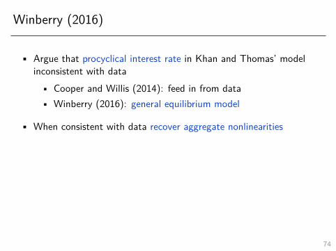
• Argue that procyclical interest rate in Khan and Thomas’ modelinconsistent with data
• Cooper and Willis (2014): feed in from data• Winberry (2016): general equilibrium model
• When consistent with data recover aggregate nonlinearities
� (rt) � (rt ; yt�1) � (rt ; yt) � (rt ; yt+1)
T-bill 2.18% -0.08 -0.17 -0.251AAA 2.34% -0.29 –0.37 -0.40BAA 2.43% -0.32 -0.41 -0.45Stock 24.7% -0.24 -0.14 0.02RBC 0.16% 0.61 0.97 0.74
74

Winberry (2016)
• Argue that procyclical interest rate in Khan and Thomas’ modelinconsistent with data
• Cooper and Willis (2014): feed in from data• Winberry (2016): general equilibrium model
• When consistent with data recover aggregate nonlinearities
� (rt) � (rt ; yt�1) � (rt ; yt) � (rt ; yt+1)
T-bill 2.18% -0.08 -0.17 -0.251AAA 2.34% -0.29 –0.37 -0.40BAA 2.43% -0.32 -0.41 -0.45Stock 24.7% -0.24 -0.14 0.02RBC 0.16% 0.61 0.97 0.74
74
Model
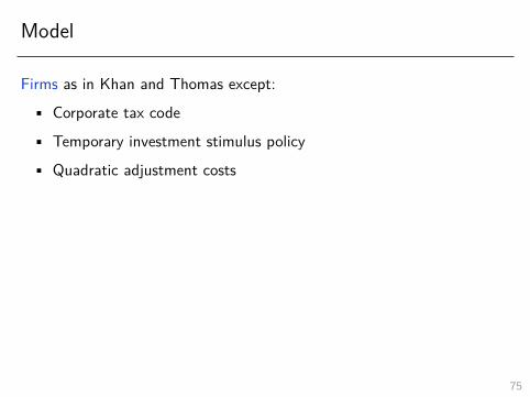
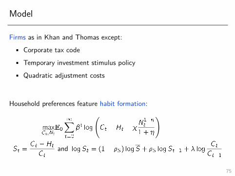
Firms as in Khan and Thomas except:• Corporate tax code• Temporary investment stimulus policy• Quadratic adjustment costs
Household preferences feature habit formation:
maxCt ;Nt
E0
1∑t=0
�t log
(Ct �Ht � �
N1+�t
1 + �
)
St =Ct �Ht
Ctand logSt = (1� �S) logS + �S logSt�1 + � log
Ct
Ct�1
75
Model
Firms as in Khan and Thomas except:• Corporate tax code• Temporary investment stimulus policy• Quadratic adjustment costs
Household preferences feature habit formation:
maxCt ;Nt
E0
1∑t=0
�t log
(Ct �Ht � �
N1+�t
1 + �
)
St =Ct �Ht
Ctand logSt = (1� �S) logS + �S logSt�1 + � log
Ct
Ct�1
75

Calibration
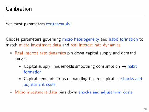
Set most parameters exogeneously
Choose parameters governing micro heterogeneity and habit formation tomatch micro investment data and real interest rate dynamics
• Real interest rate dynamics pin down capital supply and demandcurves
• Capital supply: households smoothing consumption ! habitformation
• Capital demand: firms demanding future capital ! shocks andadjustment costs
• Micro investment data pins down shocks and adjustment costs
76
Calibration
Set most parameters exogeneously
Choose parameters governing micro heterogeneity and habit formation tomatch micro investment data and real interest rate dynamics
• Real interest rate dynamics pin down capital supply and demandcurves
• Capital supply: households smoothing consumption ! habitformation
• Capital demand: firms demanding future capital ! shocks andadjustment costs
• Micro investment data pins down shocks and adjustment costs
76

Calibration
76

Calibration
76

State Dependence of Stimulus Policy
price of investment = 1� subt
77

Increasing Cost Effectiveness of Policy
subjt = �1 � n�2jt
78

Conclusion: Takeaways from Topic 2
1. Investment is lumpy in the microdata
2. Structural micro models provide evidence for nonconvex adjustmentcosts
• SMM estimation
3. Calibrated macro models indicate possibly generates time-varyingaggregate elasticity
• Aggregation and general equilibrium both important• Solving models with distribution in state vector
79
![Welcome 1 [kirtoninlindseytownhall.co.uk]...white labels 2” x 1” (5cm. x 2.5cm) positioned 1” (2.5cm) from the bottom of the bottle. Special rules for Class A23 and C20 are included](https://img.dokumen.tips/doc/110x75/5f0c70e37e708231d4356a58/welcome-1-kir-white-labels-2a-x-1a-5cm-x-25cm-positioned-1a-25cm.jpg)


![5cr+ lcm 5mm 2.5cm 24 2.5cm lcm 26cm 26cm 16cm 3.5cm lcm … · 2019-08-06 · .5cr+ lcm 5mm 2.5cm 24 2.5cm lcm 26cm 26cm 16cm 3.5cm lcm vol. : 10 era 19.5cm 25cm [7] (A4#4ÃL1-E)](https://img.dokumen.tips/doc/110x75/5f56c58c967c2a15a3138f0b/5cr-lcm-5mm-25cm-24-25cm-lcm-26cm-26cm-16cm-35cm-lcm-2019-08-06-5cr-lcm.jpg)