23rd International Meshing Roundtable (IMR23) … · Towards FEA over Tangled Quads Chaman Singh Vermaa, Krishnan Sureshb aDepartment of Computer Sciences, University of Wisconsin,

Available online at www.sciencedirect.com

Procedia Engineering 00 (2014) 000–000www.elsevier.com/locate/procedia

23rd International Meshing Roundtable (IMR23)

Towards FEA over Tangled QuadsChaman Singh Vermaa, Krishnan Sureshb

aDepartment of Computer Sciences, University of Wisconsin, Madison, WI 53705, USAbDepartment of Mechanical Engineering, University of Wisconsin, Madison, WI 53705, USA

Abstract

In finite element analysis (FEA), a mesh is said to be tangled if it contains an element with negative Jacobian-determinant. Tanglingcan occur during mesh optimization and mesh morphing. Modern FEA unfortunately cannot handle such tangled meshes, i.e., it willlead to erroneous results. While significant progress has been made on untangling, there are no definitive untangling algorithms.

Danczyk and Suresh recently proposed a theoretical extension to FEA such that one could accurately solve boundary valueproblems over such tangled meshes. However, their investigation was limited to simplicial meshes.

In this paper we consider the extension of the above framework to tangled quad meshes that pose additional challenges comparedto simplicial meshes. These challenges are identified, and a tangling-framework is developed to address explicit quad tanglingwhere quads are allowed to overlap, but are required to be geometrically convex. Numerical examples illustrate the correctness ofthe proposed framework, opening new opportunities for meshing algorithms.c© 2014 The Authors. Published by Elsevier Ltd.Peer-review under responsibility of organizing committee of the 23rd International Meshing Roundtable (IMR23).

Keywords: Tangled mesh; inverted elements; FEM

1. Introduction

In modern finite element analysis (FEA), the underlying mesh is required to: (1) be simply connected, (2) conformto the boundary, (3) be of good quality, and (4) not contain inverted elements [14,19]. The focus of this paper is oninverted elements; Figure 1 illustrates a mesh containing an inverted element.

Mathematically, an element is inverted if the determinant of its Jacobian is negative. Furthermore, a mesh contain-ing inverted elements is said to be tangled. Element-inversion and tangling can occur during mesh-generation [12],mesh-optimization [8,9], morphing [17] and large-scale deformation [18].

Modern finite element theory is incapable of handling such tangled meshes. Any implementation based on existingtheory will lead to erroneous results. For example, relative error in the order of 1000% can be observed in some cases(see example below). Given such evidence, researchers and practitioners today unanimously recommend untangling

∗ Corresponding author. Tel.: +0-608-698-4729E-mail address: [email protected]

1877-7058 c© 2014 The Authors. Published by Elsevier Ltd.Peer-review under responsibility of organizing committee of the 23rd International Meshing Roundtable (IMR23).

2 Chaman Singh Verma, Krishnan Suresh / Procedia Engineering 00 (2014) 000–000

Fig. 1: A quad mesh inverted/tangled elements

prior to analysis. For example, to quote [2]: “Because tangled meshes generate physically invalid solutions, it isimperative that such meshes [be] untangled”.

While there has been significant progress on untangling [10], it can be as difficult as mesh generation [15]. Forexample, to quote [11]: “Although there is a O(n) complexity algorithm to detect the presence of tangle elements,there are no known a priori test to determine if a mesh can be untangled”.

To overcome this dilemma, Danczyk and Suresh recently proposed a new theoretical extension to finite elementanalysis for handling tangled simplicial (triangle and tetrahedral) meshes. The proposed framework offers a novelapproach for carrying out accurate finite element analysis over a tangled simplicial mesh [6,7] As an illustrativeapplication of their framework, consider solving a linear elasticity problem over a unit square in Figure 2a. Theboundary conditions are given by

u(x, y) = 0.1x − 0.2y

v(x, y) = 0.3x + 0.5y (1)

with zero body force. Since the boundary conditions are linear, the exact solution over the entire domain is also givenby Equation (1)

If one uses a non-tangled mesh, as in Figure 2a, the exact solution is recovered (to within machine precision)through classic FEA.

On the other hand, consider a tangled mesh in Figure 2b that was artificially created by moving nodes 6 and 7towards each other. In this configuration, there are six positive elements, two inverted elements, and 15 overlappingpair of elements.

Fig. 2: (a) A non-tangled simplicial mesh, (b) tangled mesh.

The above problem was solved over the tangled mesh using both the classic FEA and tangled FEA, for variousconfigurations of the mesh. As one can observe in Figure 3, using classic FEA, the relative error at node-6 reachesan astounding 3500% in the final configuration. On the other hand, using the tangled FEA proposed by Danczyk andSuresh [6], the error is within machine precision for all positions (barring the singular positions when node 6 coincideswith node 7). Additional examples can be found in [6,7].

The objective of this paper is to extend the above tangled FEA framework to quadrilateral meshes, since tanglingis much more common in such meshes. Our intention is to lay the foundation for FEA over tangled hex meshes, wheretangling is a serious problem.

Chaman Singh Verma, Krishnan Suresh / Procedia Engineering 00 (2014) 000–000 3

Fig. 3: Relative errors at node-6 using classic-FEA and tangled FEA.

2. FEA over Tangled Quad Meshes

We briefly review the basic theory of FEA over quad meshes, followed by an analysis of quad tangling.

2.1. Quad Element Shape Functions

Four-noded quad elements, with two degrees of freedom at each node, are used extensively in 2D linear elasticity.The most basic four-node formulation is the bi-linear iso-parametric formulation [5,19] illustrated in Figure 4, wherefour functions are defined, each associated with one of the four corners:

N1(ξ, η) =14

(1 − ξ)(1 − η)

N2(ξ, η) =14

(1 + ξ)(1 − η)

N3(ξ, η) =14

(1 + ξ)(1 + η)

N4(ξ, η) =14

(1 − ξ)(1 + η) (2)

Using these shape functions, one can map a standard point (ξ, η) to a physical point (x, y) via (see Figure 4):

x(ξ, η) =

4∑i=1

Ni(ξ, η)xi y(ξ, η) =

4∑i=1

Ni(ξ, η)yi (3)

where xi & yi are the coordinates of the four nodes.Given the above transformation, the Jacobian is defined as:

J =

∂x∂ξ

∂x∂η

∂x∂ξ

∂x∂η

(4)

The Jacobian plays a crucial role, for example, in transforming integrals:∫f (x, y)dxdy =

∫f (ξ, η)|J|dξdη (5)

The inverse of the Jacobian plays a role in transforming gradients:

∇xy(·) = J−T∇ξη(·) (6)


Fig. 4: Isoparametric mapping

Similar to Equation (3), the field over an element is interpolated via:

u(ξ, η) =

4∑i=1

Ni(ξ, η)uei = Nue (7)

where uei are field values associated with the four nodes. Thus, to compute the value of field at a point: (1) first the

element the point belongs to is determined, and (2) then the sum of contributions from all four nodes of that elementis evaluated.

The field description in Equation (7) satisfies a continuity property in the following sense. Consider, edge 1-2corresponding to η = −1; from Equation (2) and (7), we have:

u(ξ,−1) = 0.5((1 − ξ)u1 + (1 + ξ)u2) (8)

Thus the field on this edge depends only the nodal values of 1 and 2. A similar analysis can be established for aneighboring element. It therefore follows that the field is continuous across the entire mesh. Unfortunately, thisessential property breaks down when the mesh is tangled

2.2. Challenges posed by Tangling

To understand the impact of tangling on the continuity of the field, consider a node and a set of quad elementssurrounding it as illustrated in Figure 5a. Let the field value at node-1 be 1, and the value at all other nodes be 0. Theresulting field is a hat function illustrated in Figure 5b. From the continuity of the field across element boundaries(see previous Section), it follows that the hat function is continuous. Further, since the global field is simply a linearcombination of such hat functions, the global continuity is established.

Fig. 5: (a) Non-tangled mesh, and (b) a hat function

Now consider a scenario of tangling where elements 1 & 2 flip over as illustrated in Figure 6b. On the overlappingregion, points belong to multiple elements; therefore the hat-function is multiple-valued and is ill-defined. Further,one can easily deduce that the hat function will not be continuous across, say edge 3-4. Thus a fundamental premiseof continuous Galerkin FEA is violated, and consequently, erroneous FEA results can be expected.

2.3. Self-Tangling of a Concave and Twisted Quads

Figure 6b, illustrated above, is an example of explicit tangling where elements overlap with each other. In addition,quad-meshes can also exhibit self-tangling or implicit tangling. For example, consider the quad mesh in Figure 7a,


Fig. 6: (a) Non-tangled mesh, and (b) tangled mesh

consisting of five convex quads. By rotating the center quad, the remaining four quads become concave as in Figure7b. Clearly, none of the elements geometrically overlap with each other, i.e., there is no explicit tangling. However,each of the four concave elements is self-tangled for reasons explained below.

Fig. 7: (a) A valid mesh, and (b) a mesh with concave (self-tangled) elements.

Consider again the bilinear parametric mapping of Equation (3), but onto a concave quad element where thereentrant vertex is located at (1/3, 1/3) (see Figure 8a). Given the coordinates of this element, one can show viaEquation (3) that the parametric mapping is given by:

x(ξ, η) =5 + 5ξ − 3η − 3ξη

16

y(ξ, η) =5 − 5ξ + 5η − 3ξη

16(9)

One can now verify that two points a(ξ, η) = (0, 0) and b(ξ, η) = (2/3, 2/3) map to the same physical point (5/16,5/16); see Figure 8. Thus the parametric mapping is not invertible. This, by itself, poses serious challenges duringGaussian integration. Further, observe that the determinant of the Jacobian for the above mapping is given by:

Fig. 8: A simplicial mesh with an inverted element

|J| =2 − 3ξ − 3η

32(10)


The determinant vanishes over the line 2 − 3ξ − 3η = 0, dividing the parametric space into a + region where thedeterminant |J| is positive, and a - region where |J| is negative (see Figure 9a). The corresponding physical regionsare illustrated in Figure 9b and Figure 9c. Observe that these two regions overlap (fold) outside the concave geometryof the quad. While this fold is visually hidden, it mathematically exists, and it overlaps with the neighboring quad aswell! Similarly, consider the twisted quad illustrated in Figure 10a. One can show that the quad element overlaps with

Fig. 9: (a) Parametric space is divided into positive and negative regions, (b) the mapping of the two regions, and (c) final physical space isself-overlapping.

itself (see Figure 10b) and with its neighbors. Self-overlapping is difficult to handle mathematically and numerically.

Fig. 10: (a) Intended twisted quad, and (c) self-overlapping region.

It may be possible to handle such elements through non-standard parametric mapping (for example see [4,13]), butthis is a topic of future research. Therefore, for the remainder of this paper, we focus on tangled quad meshes whereelements may explicitly overlap with each other, but all elements are geometrically convex.

2.4. FEA over Tangled Quad Meshes: Theory

We now address FEA over a tangled quad mesh where all elements are geometrically convex, i.e., the Jacobiandeterminant |J| is either entirely positive or entirely negative over each element. The strategy is to arrive at a modifieddescription of the global field that is consistent, unambiguous and continuous over a tangled mesh; this will lead us tothe modified FEA formulation for a tangled mesh. Towards this end, we extend the framework proposed by Danczykand Suresh [6,7], starting with the following definitions.

Definition 1: Let θk be the sign of the Jacobian determinant |J| for element k.


Definition 2: Let the index associated with any point in the mesh be the set of elements the point belongs to

I(p) = k | p ∈ Ek (11)

The notion of an index leads naturally to the concept of a cell.Definition 3: A cell is the set of all points with identical index .Figure 11c illustrates five distinct cells induced by tangling. Observe that a cell need not be convex, or even

connected. Further, while there may be other quads that overlap with the four quads shown, we only focus on thequads attached to node-1 since the focus is on a hat function associated with node 1.

Fig. 11: (a) Non-tangled mesh, (b) tangled mesh, and (c) cells induced.

Now define a cell shape function S α over each cell as follows:

S α(p) =∑

k∈Iα(p)

θkNk(p) (12)

In the above equation, Nk is the unique shape function (among the four) that takes a value of 1 at node-1 forelement-k. Thus at any point in the mesh, the value of the cell shape function is a linear combination of all thestandard element shape functions associated with that cell, weighted by the orientation of the element. Observe thatcell shape functions are uniquely defined by construction. Further, the following theorem establishes their continuity.

Theorem: The cell shape functions defined via Equation (12) satisfy the following properties: (1) they are contin-uous across cell-boundaries, and (2) they vanish on the boundary of the cell complex.

Proof: The proof is an extension of the one in [6,7] for simplicial mesh. Consider the first part of the proof; letCα&Cβ be two neighboring cells, with indices Iα&Iβ. It must be proven that the cell shape functions S α(·) and S β(·)are continuous across the common boundary. To this end, consider the difference between the two functions S α − S β;one can group the terms into three categories:

S α − S β =∑

k∈Iα∩Iβ

[< 1 >] +∑

k∈Iα−Iβ

[< 2 >] +∑

k∈Iβ−Iα

[< 3 >]

The first term contains the contribution from every element k that belongs to both Iα&Iβ. For every such element,Nk is continuous across the common boundary, therefore the first term vanishes on the boundary, independent of theorientation θk. Next consider an element k in the second term, i.e., the element is in Iα but not in Iβ. This implies ithat in crossing from Cα to Cβ, we must exit element Ek. Observe that exiting Ek can only occur in two ways: (1)simultaneously exit ω, or (2) enter a neighboring element E j. In the first case, Nk is necessarily zero at the boundaryof point of ω. Therefore, all such contributions vanish from the second term. In the second case of exiting Ek andentering one of its neighbors E j, there are again two cases: (2a) Ek and E j are of the same orientation, and (2b)Ek and E j are of opposite orientation. If the elements are of the same orientation, then E j must belong to Cβ, andθkNk = θ jN j. Therefore these contributions vanish from the 2nd term. Finally, if Ek and E j are of opposite orientation,then E j must also belong to Cα, therefore θkNk + θ jN j = θkNk − θkN j, which also vanishes since the two elementfunctions are continuous at that point. Through a similar argument, the third term also vanishes. Thus S α(·) and S β(·)are continuous across the common boundary.

Now consider the second part of the proof where it must be shown that if Cα intersects the boundary of ω, then S α

is necessarily zero on the boundary. Observe that the boundary of any Cα must is also the boundary of at least oneelement Ek. Since we are exiting Cα, we must also be exiting the element Ek. Once again, exiting Ek can only occur


in two ways: (1) simultaneously exit ω, or (2) enter a neighboring element E j. In the first case, iNkis necessarily zeroat the boundary of point of ω. In the second case Ek and E j must necessarily be of opposite orientation (since we arealso exiting ω). As before, the contributions from both elements cancel out at such boundary points, and therefore, S α

vanishes.Finally, due to the quasi-disjoint decomposition and continuity, the cell shape functions S α can be stitched together

to define a continuous hat-function at a node. Since a point belongs to a unique cell, the field is defined via the cellshape function as:

u(p) =∑

k∈Iα(p)

θkNk(p)uk (13)

The reader may wish to compare Equations (13) and (7). Thus, to find the value of field at a point in a tangled mesh:(1) find the set of element the point belongs to, and (2) evaluate the sum of contributions from all elements, weightedby the orientation of that element. The global field is now uniquely defined, and is continuous across the entire mesh.

2.5. FEA over Tangled Quad Meshes: Linear Algebra

While the concepts of cells and cell shape functions are crucial to establishing the proposed framework, they arenot computed explicitly for the following reason. For example, consider the Poisson problem:∫

Ω

∇u.∇v =

∫Ω

vdΩ (14)

Substituting Equation (13) in above:∫Ω

∇

∑k∈Iα(p)

θkN(p)uk

.∇ ∑

j∈Iα(p)

θ jN(p)vj

dΩ =

∫Ω

∑k∈Iα(p)

θkN(p)vk

dΩ (15)

Pushing the gradient inside the summation:∫Ω

∑k∈Iα(p)

θk∇Nuk

. ∑

j∈Iα(p)

θ j∇Nvj

dΩ =

∫Ω

∑k∈Iα(p)

θkNvk

dΩ (16)

Since N is zero outside the corresponding element k, we have: ∑k∈Iα(p)

∫Ωk

θk∇NukdΩ

.∑

j∈Iα(p)

∫Ω j

θ j∇NvjdΩ

=∑

k∈Iα(p)

∫Ωk

θkNvkdΩ (17)

Expanding the terms on the left hand side, and regrouping, we have: ∑k∈Iα(p)

∫Ωk

θkθk∇Nuk.∇NvkdΩ

+

∑

k, j∈Iαk, j

∫Ωk∩Ω j

θkθ j∇Nuk∇NvjdΩ

=

∑k∈α(p)

∫Ωk

θkNvkdΩ

(18)

Since:

(θk)2 = 1 (19)

we arrive at the following linear system of equations:

(Kclassic + Koverlapping)u = foriented (20)


where

Kclassic =∑

Assemble

∫Ωk

∇N.∇NdΩ

Koverlapping =∑

Assemble

∫Ω j∩Ωk

θkθ j∇N j.∇NkdΩ (21)

foriented =∑

Assemble

∫Ω j

θkNdΩ

The assembly in Equation (21) is the standard finite element assembly, described for example, in [19]Observe that if there are no overlaps, then Equation (21)b is identically zero. In addition, in a non-tangled mesh,

all elements are necessarily positively oriented, and therefore the forcing term in Equation (21)c reduces to the classicforcing term, i.e., classic FEA is exactly recovered. While the above derivation targets 2-D Poisson equation, it canbe easily generalized to other elliptic equations. Numerical examples later illustrate the validity the method for 2-Dlinear elasticity.

2.6. FEA over Tangled Quad Meshes: Implementation

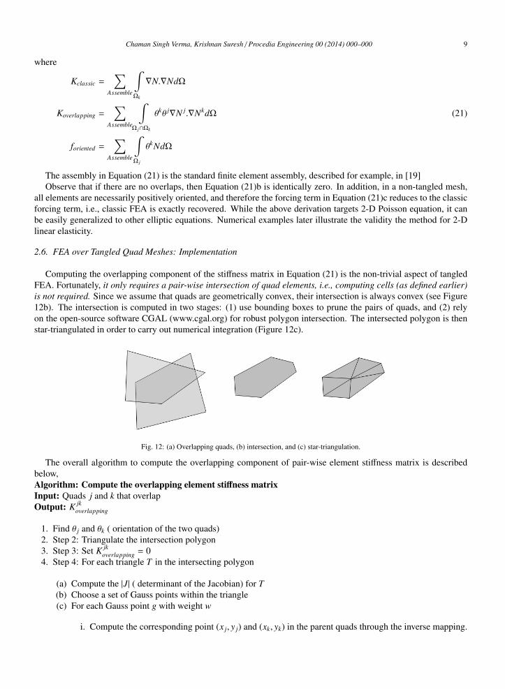
Computing the overlapping component of the stiffness matrix in Equation (21) is the non-trivial aspect of tangledFEA. Fortunately, it only requires a pair-wise intersection of quad elements, i.e., computing cells (as defined earlier)is not required. Since we assume that quads are geometrically convex, their intersection is always convex (see Figure12b). The intersection is computed in two stages: (1) use bounding boxes to prune the pairs of quads, and (2) relyon the open-source software CGAL (www.cgal.org) for robust polygon intersection. The intersected polygon is thenstar-triangulated in order to carry out numerical integration (Figure 12c).

Fig. 12: (a) Overlapping quads, (b) intersection, and (c) star-triangulation.

The overall algorithm to compute the overlapping component of pair-wise element stiffness matrix is describedbelow,Algorithm: Compute the overlapping element stiffness matrixInput: Quads j and k that overlapOutput: K jk

overlapping

1. Find θ j and θk ( orientation of the two quads)2. Step 2: Triangulate the intersection polygon3. Step 3: Set K jk

overlapping = 04. Step 4: For each triangle T in the intersecting polygon

(a) Compute the |J| ( determinant of the Jacobian) for T(b) Choose a set of Gauss points within the triangle(c) For each Gauss point g with weight w

i. Compute the corresponding point (x j, y j) and (xk, yk) in the parent quads through the inverse mapping.


ii. Compute the shape derivatives ∇N j and ∇NK at (x, y)iii. K jk

overlapping+ = wθ jθ j∇N j.∇Nk |J|

3. Numerical Experiments

In all numerical experiments, we solve 2-D linear elasticity problems with zero body force. The material propertiesare as follows: E (Youngs modulus) = 100 GPa, and (Poissons ratio) = 0.25; the boundary conditions are describedunder each experiment. The main objective of these experiments is to compare the accuracy of classic FEA againsttangled FEA.

3.1. Experiment-1: Triangle Splitting with Analytic Solution

The first experiment mirrors the experiment summarized in Figure 2, except that each triangle is split into fourquads (see Figure 13a). The boundary conditions are given by Equation (1) with zero body force. Each side of thesquare is 1 unit; in Figure 13a nodes 6 and 7 are at 0.25 and 0.75 units respectively. The boundary conditions are suchthat the exact solution is given by Equation (1). Now consider moving the nodes 6 and 7 to their new positions inFigure 13b (where node 6 is at 0.6 and node 7 is at 0.4), while maintaining the convexity of the underlying trianglesand quads. The resulting quad-mesh has all convex elements by construction, but is tangled with six inverted quadelements as illustrated. One can identify and visualize the inverted elements by referring to the numbering of Figure13a, and tracing the quads in Figure 13b.

Fig. 13: (a) Non-tangled mesh, and (b) tangled mesh

The above problem (non-tangled and tangled) was solved via classic FEA and tangled FEA for various configura-tions of node 6 and node 7 as illustrated in Figure 14 (except for the singular position when nodes 6 and 7 coincide).The relative error at node-6 is summarized in Figure 14. Observe that the error in classical FEA reaches an astounding5000%, while tangled-FEA was found to be accurate to within 0.0001% (machine acccuracy could not be achieved;we suspect the source of error to be the inverse mapping).

3.2. Experiment-2: Chord Inversion with Analytic Solution

One can also create tangling by inverting a chain of quads. For example, consider the quad mesh in Figure 15aconsisting of four rings of node. One can induce tangling by switching the positions of the 2nd and 3rd ring of nodes,while maintaining the quad connectivity. The resulting tangled quad mesh is illustrated in Figure 15b, where the 2ndlayer of quads in now inverted. The inversion can be confirmed by referring to the numbering of Figure 15a, andtracing the quads in Figure 15b.

The above method is now applied to the quad mesh in Figure 16a. Specifically, the 4th layer of quads is invertedvia a parameter where corresponds to no tangling, while corresponds to full tangling as in Figure 16b.

For each configuation of the mesh, the exact problem given by Equation (1) was solved via classic FEA and tangledFEA for each configuration of the mesh (except for the singular position where the two chains of nodes coincides).


Fig. 14: Numerical results for the problem posed in Figure 13.

Fig. 15: (a) Non-tangled mesh, and (b) tangled mesh.

Fig. 16: (a) Non-tangled mesh, and (b) tangled mesh.

Fig. 17: (a) Numerical results for the problem posed in Figure 16. (b) Condition number for the problem posed in Figure 16.

The relative error is summarized in Figure 17. Once again, observe a highly accurate result for tangled FEA, whileclassical FEA exhibits significant error with increasing levels of tangling (when ).


For the above problem, the condition number of the stiffness matrices 20 was computed for each configuation of themesh. As one can observe in Figure 17b, the condition numbers for both methods are identical. Further, the conditionnumber blows up as as expected since this correponds to a mesh with degenerate quads.

3.3. Experiment-3: Quad Inversion with Non-Analytic Solution

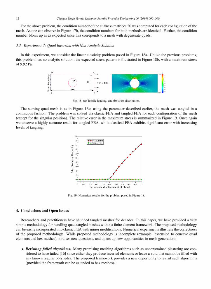
In this experiment, we consider the linear elasticity problem posed in Figure 18a. Unlike the previous problems,this problem has no analytic solution; the expected stress pattern is illustrated in Figure 18b, with a maximum stressof 9.92 Pa.

Fig. 18: (a) Tensile loading, and (b) stress distribution.

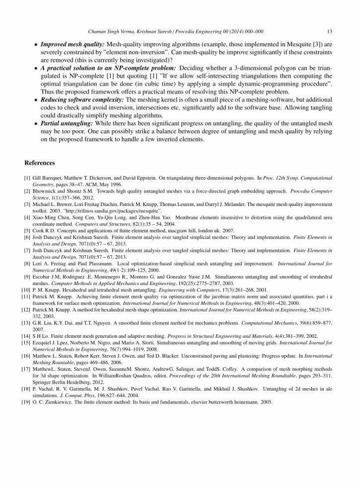
The starting quad mesh is as in Figure 16a; using the parameter described earlier, the mesh was tangled in acontinuous fashion. The problem was solved via classic FEA and tangled FEA for each configuration of the mesh(except for the singular position). The relative error in the maximum stress is summarized in Figure 19. Once againwe observe a highly accurate result for tangled FEA, while classical FEA exhibits significant error with increasinglevels of tangling.

Fig. 19: Numerical results for the problem posed in Figure 18.

4. Conclusions and Open Issues

Researchers and practitioners have shunned tangled meshes for decades. In this paper, we have provided a verysimple methodology for handling quad tangled meshes within a finite element framework. The proposed methodologycan be easily incorporated into classic FEA with minor modifications. Numerical experiments illustrate the correctnessof the proposed methodology. While proposed methodology is incomplete (example: extension to concave quadelements and hex meshes), it raises new questions, and opens up new opportunities in mesh generation:

• Revisiting failed algorithms: Many promising meshing algorithms such as unconstrained plastering are con-sidered to have failed [16] since either they produce inverted elements or leave a void that cannot be filled withany known regular polyhedra. The proposed framework provides a new opportunity to revisit such algorithms(provided the framework can be extended to hex meshes).


• Improved mesh quality: Mesh-quality improving algorithms (example, those implemented in Mesquite [3]) areseverely constrained by ”element non-inversion”. Can mesh-quality be improve significantly if these constraintsare removed (this is currently being investigated)?

• A practical solution to an NP-complete problem: Deciding whether a 3-dimensional polygon can be trian-gulated is NP-complete [1] but quoting [1] ”If we allow self-intersecting triangulations then computing theoptimal triangulation can be done (in cubic time) by applying a simple dynamic-programming procedure”.Thus the proposed framework offers a practical means of resolving this NP-complete problem.

• Reducing software complexity: The meshing kernel is often a small piece of a meshing-software, but additionalcodes to check and avoid inversion, intersections etc. significantly add to the software base. Allowing tanglingcould drastically simplify meshing algorithms.

• Partial untangling: While there has been significant progress on untangling, the quality of the untangled meshmay be too poor. One can possibly strike a balance between degree of untangling and mesh quality by relyingon the proposed framework to handle a few inverted elements.

References

[1] Gill Barequet, Matthew T. Dickerson, and David Eppstein. On triangulating three-dimensional polygons. In Proc. 12th Symp. ComputationalGeometry, pages 38–47. ACM, May 1996.

[2] Bhowmick and Shontz S.M. Towards high quality untangled meshes via a force-directed graph embedding approach. Procedia ComputerScience, 1(1):357–366, 2012.

[3] Michael L. Brewer, Lori Freitag Diachin, Patrick M. Knupp, Thomas Leurent, and Darryl J. Melander. The mesquite mesh quality improvementtoolkit. 2003. ”http://trilinos.sandia.gov/packages/mesquite”.

[4] Xiao-Ming Chen, Song Cen, Yu-Qiu Long, and Zhen-Han Yao. Membrane elements insensitive to distortion using the quadrilateral areacoordinate method. Computers and Structures, 82(1):35 – 54, 2004.

[5] Cook R D. Concepts and applications of finite element method, macgraw hill, london uk. 2007.[6] Josh Danczyk and Krishnan Suresh. Finite element analysis over tangled simplicial meshes: Theory and implementation. Finite Elements in

Analysis and Design, 7071(0):57 – 67, 2013.[7] Josh Danczyk and Krishnan Suresh. Finite element analysis over tangled simplicial meshes: Theory and implementation. Finite Elements in

Analysis and Design, 7071(0):57 – 67, 2013.[8] Lori A. Freitag and Paul Plassmann. Local optimization-based simplicial mesh untangling and improvement. International Journal for

Numerical Methods in Engineering, 49(1-2):109–125, 2000.[9] Escobar J.M, Rodriguez .E, Montenegro R., Montero G, and Gonzalez Yuste J.M. Simultaneous untangling and smoothing of tetrahedral

meshes. Computer Methods in Applied Mechanics and Engineering, 192(25):2775–2787, 2003.[10] P. M. Knupp. Hexahedral and tetrahedral mesh untangling. Engineering with Computers, 17(3):261–268, 2001.[11] Patrick M. Knupp. Achieving finite element mesh quality via optimization of the jacobian matrix norm and associated quantities. part i a

framework for surface mesh optimization. International Journal for Numerical Methods in Engineering, 48(3):401–420, 2000.[12] Patrick M. Knupp. A method for hexahedral mesh shape optimization. International Journal for Numerical Methods in Engineering, 58(2):319–

332, 2003.[13] G.R. Liu, K.Y. Dai, and T.T. Nguyen. A smoothed finite element method for mechanics problems. Computational Mechanics, 39(6):859–877,

2007.[14] S H Lo. Finite element mesh generation and adaptive meshing. Progress in Structural Engineering and Materials, 4(4):381–399, 2002.[15] Ezequiel J. Lpez, Norberto M. Nigro, and Mario A. Storti. Simultaneous untangling and smoothing of moving grids. International Journal for

Numerical Methods in Engineering, 76(7):994–1019, 2008.[16] Matthew L. Staten, Robert Kerr, Steven J. Owen, and Ted D. Blacker. Unconstrained paving and plastering: Progress update. In International

Meshing Rountable, pages 469–486, 2006.[17] MatthewL. Staten, StevenJ. Owen, SuzanneM. Shontz, AndrewG. Salinger, and ToddS. Coffey. A comparison of mesh morphing methods

for 3d shape optimization. In WilliamRoshan Quadros, editor, Proceedings of the 20th International Meshing Roundtable, pages 293–311.Springer Berlin Heidelberg, 2012.

[18] P. Vachal, R. V. Garimella, M. J. Shashkov, Pavel Vachal, Rao V. Garimella, and Mikhail J. Shashkov. Untangling of 2d meshes in alesimulations. J. Comput. Phys, 196:627–644, 2004.

[19] O. C. Zienkiewicz. The finite element method: Its basis and fundamentals, elsevier butterworth heinemann. 2005.

Documents

23rd International Meshing Roundtable (IMR23) … · Towards FEA over Tangled Quads Chaman Singh Vermaa, Krishnan Sureshb aDepartment of Computer Sciences, University of Wisconsin,