Available online at www.sciencedirect.com

Procedia Engineering 00 (2014) 000–000www.elsevier.com/locate/procedia

23rd International Meshing Roundtable (IMR23)

Automatic Unstructured Element-Sizing Specification Algorithm forSurface Mesh Generation

Zhoufang Xiao, Jianjun Chen∗, Yao Zheng, Lijuan Zeng, Jianjing Zheng

Center for Engineering and Scientific Computation,and School of Aeronautics and Astronautics, Zhejiang University, Hangzhou 310027, China

Abstract

Automatic and accurate element-sizing specification is crucial for the efficient generation of surface meshes with a reduced numberof elements. This study proposes a novel algorithm to fulfill this goal, which is based on the unstructured background mesh, andprovides an alternative of existing Cartesian mesh based algorithms. The geometric factors are considered and combined withsome user parameters to form an initial size map. This map is then smoothed to a well-graded one. The timing efficiency of thesize-query routine is improved to a comparable level with that based on the Cartesian mesh. Finally, the size map produced by theproposed algorithm is used to control the scales of elements generated by an advancing front surface mesher. Meshing experimentsof complex computational aerodynamics configurations show that the proposed algorithm only consumes minutes to prepare thesize map for the surface mesher; however, a conventional grid sources based scheme may need many hours by a tedious manualinteraction process.c© 2014 The Authors. Published by Elsevier Ltd.Peer-review under responsibility of organizing committee of the 23rd International Meshing Roundtable (IMR23).

Keywords: Mesh generation; Surface mesh; Element size; Adaptive mesh; Background mesh

1. Introduction

In the community of computational aerodynamics, a great success of unstructured mesh technologies has beenwitnessed in the past decades due to its automatic and adaptive abilities for complex geometry configurations [1].Nowadays, many commercial or in-house codes can generate unstructured meshes in a very reliable and computa-tionally efficient manner. Owing to the rapid advance of parallel mesh generation algorithms, the time cost consumedby the pipeline of unstructured mesh generation can be further reduced to a very low level [2–5]. For instance, theauthors have recently implemented a parallel pipeline where the three major steps of unstructured mesh generation(i.e., surface meshing, volume meshing and volume mesh quality improvement) are all parallelised [4,5]. Experimentsshow that this parallelised pipeline can employ about 100 computer cores to generate a high-quality mesh composedof hundreds of millions of tetrahedral elements in minutes.

∗ Corresponding author. Tel.: +0-086-571-87951883 ; fax: +0-086-571-87953168.E-mail address: chenjj@zju.edu.cn

1877-7058 c© 2014 The Authors. Published by Elsevier Ltd.Peer-review under responsibility of organizing committee of the 23rd International Meshing Roundtable (IMR23).

2 Z. Xiao, J. Chen and Y. Zheng et al. / Procedia Engineering 00 (2014) 000–000

Although the pipeline of unstructured mesh generation might not be a performance bottleneck any more in manycases, how to prepare a valid and suitable input for this meshing pipeline remains challengeable. In general, this inputcontains a geometry that defines the meshing domain and an element-sizing function that defines the distribution ofelement scales over the meshing domain. In the following discussions, our focus is only on the preparation of theelement-sizing function for unstructured surface mesh generation. The preparation of a high-quality geometry inputis not discussed in this study. However, it needs to be emphasised that this issue is a very active research topic in thecommunity of mesh generation [6].

A good element-sizing function should define small element scales in the region where geometrical and physicalcharacteristics exist and large scales elsewhere. Moreover, the gradation of the element scales must be limited so thatthe quality of elements in the gradation region is ensured. In the community of computational aerodynamics, gridsources are popular tools and employed by many meshing codes to define element-sizing functions [7–10]. For asimple configuration such as the DLR-F6 wing-body-nacelle-pylon aircraft (referred to as the F6 model hereafter),tens of grid sources are enough to help generate a good-quality surface mesh for typical aerodynamics simulations.The time cost of defining the sources of this magnitude is usually affordable if a user friendly graphic interface isavailable. However, if a more complicated aerodynamics model such as a full loaded fight aircraft is input, more thanhundreds of grid sources might be required, and the interactive process that defines these sources is error-prone andtime-consuming. In our experience, even days of wall-clock time might be consumed. By contrast, the subsequentautomatic meshing pipeline consumes only minutes of wall-clock time. In this sense, if not considering the geometrypreparation step, the real performance bottleneck of generating unstructured meshes for a complicated aerodynamicsmodel lies in the phase of defining element-sizing functions rather than mesh generation itself.

For many years, solution-adaptive techniques have been expected to be able to remove the dependence of thecomputing accuracy on the initial mesh configuration. However, it was reported that an adapted solution might beinvalid if it originated from a poor-quality mesh [8]. In fact, a good initial mesh can either eliminate the need foradaptive grid refinement for certain class of problems or enhance the performance of many adaptation methods.Therefore, even configured with an adaptive solver, the requirement that defines a suitable element-sizing map for theinitial mesh generation is still indispensable.

Many automatic algorithms have been designed to define an element-sizing map in a less intensive user-interactivemanner. A fundamental feature that can be used to classify these algorithms is the background mesh adopted, wherethe element-sizing map is stored by assigning element scales at mesh nodes and interpolating scales in backgroundelement interiors using the node values. The most prevailing background mesh adopted so far is the Cartesian mesh,which is interiorly organised as a quadtree or octree; thus, the time complexity of searching a background elementthat contains a point is proportional to the depth of the tree. This fast search property is vital to reduce the meshingtime because a meshing process would call this search routine frequently. However, the disadvantage of using aCartesian mesh is that the tree-level difference of neighboring cells is required to be less than or equal to one, and therefinement of a single cell has to be propagated into its neighboring cells. Therefore, the Cartesian mesh based schemeis expensive in terms of computational time and storage requirement [7–9]. This shortcoming even became one of thereasons that Pirzadeh gave up his early Cartesian mesh based element-sizing scheme [7] when he developed a newscheme for volume meshing problem [8].

In this study, a new automatic algorithm that initialises element-sizing maps for surface mesh generation is pro-posed by using unstructured background meshes. In contrast to the Cartesian background mesh, the unstructuredmesh has a more flexible topological structure and its local update does not need to be propagated; hence, it canrepresent a size map with reduced memory and timing requirements. In addition, instead of using a volume Cartesianbackground mesh for surface mesh generation, the unstructured background mesh considered in this study is a surfacemesh. This feature can further reduce the memory and time consumption of the proposed algorithm. To highlight thecontributions of this study, some features of the proposed algorithm are listed as below:(1) Curvature and proximity features of the input geometry are calculated and element scales are adapted to these

features automatically.(2) The requirement of a well-graded size map defined on the unstructured mesh is formularised, and an automatic

procedure is suggested to limit the gradation of element scales.(3) A brute-force procedure that queries the size value of a point in an unstructured background mesh is very slow

and its practical efficiency is unacceptable. An improved query procedure that does not depend on any auxiliarystructure is suggested in this study.

Z. Xiao, J. Chen and Y. Zheng et al. / Procedia Engineering 00 (2014) 000–000 3

Furthermore, the size map produced by the proposed algorithm is used to control the scales of elements generatedby an advancing front surface mesher. Two typical aerodynamics models are tested in this article. One is the F6model, and the other is a full loaded F16 aircraft model with landing gear details. Experiment results show that theproposed algorithm can help generate high-quality surface meshes in a far more computationally efficient manner thanthe meshing process that controls element scales purely by grid sources.

2. Preliminary definitions

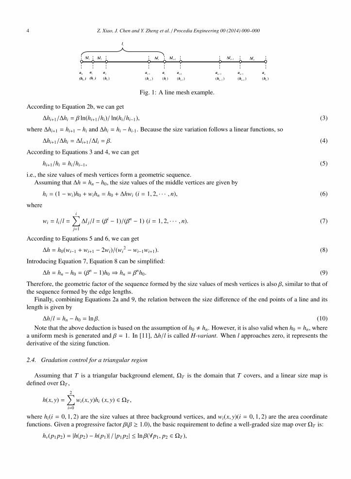
2.1. Unit mesh

As shown in Figure 1, assuming that the size function of this line is h(t)(t ∈ [0, 1]), the length of the line is l, thenumber of mesh segments in this line is:

n = l∫ 1

0

1h(t)

dt. (1a)

For each segment of this line,

1 = l∫ ti+1

ti

1h(t)

dt (i = 1, 2, · · · , n). (1b)

Given a metric M =[1/h2(t)

]defined in this line, in the space defined by M, the length of this segment is

(∆li)M =

∫ ti+1

ti

√l ·

1h2(t)

· ldt = l∫ ti+1

ti

1h(t)

dt = 1 (i = 1, 2, · · · , n),

which means that an ideal mesh edge in the space defined by M has a unit length. Correspondingly, we call this mesha unit mesh [11].

Moreover, if h(t) is a linear function, i.e., h(t) = (1 − t)h0 + thn, we can get a new equation from Equation 1a:

n =

l/h h0 = hn = hl · ln(hn/h0)/(hn − h0) h0 , hn

. (2a)

Assuming that the length of the segment ai−1ai is ∆li, for each segment of this line,

1 =

∆li/h hi = hi−1 = h∆li · ln(hi/hi−1)/(hi − hi−1) hi , hi−1

(i = 1, 2, · · · , n). (2b)

2.2. Geometric progressive mesh

For the mesh shown in Figure 1, ∀β ≥ 1.0, if

∆li+1

∆li=

β ∆li+1 ≥ ∆li1/β ∆li+1 < ∆li

(i = 1, 2, · · · , n − 1),

this mesh is called a geometric progressive mesh, and β the progressive factor. Loosely, if1β≤

∆li+1

∆li≤ β(i = 1, 2, · · · , n − 1),

this mesh is called a quasi geometric progressive mesh.

2.3. H-variant for a line

It is supposed that the mesh shown in Figure 1 meets the following assumptions: (1) It is a unit mesh, i.e., thepredefined size map is accurately respected; (2) It is a geometric progressive mesh with the progressive factor β; (3)The size variation follows a linear function.

Without loss of generality, we assume hn > h0 and

∆li+1/∆li = β (i = 1, 2, · · · , n − 1).

4 Z. Xiao, J. Chen and Y. Zheng et al. / Procedia Engineering 00 (2014) 000–000

iΔl

1

1( )

i

i

a

h

1Δl 2Δl 1iΔl 1nΔlnΔl

0

0

a

(h )

1

1

a

(h )

2

2( )

a

h ( )

i

i

a

h

1

1( )

i

i

a

h

2

2( )

n

n

a

h

1

1( )

n

n

a

h ( )

n

n

a

h

il

Fig. 1: A line mesh example.

According to Equation 2b, we can get

∆hi+1/∆hi = β ln(hi+1/hi)/ ln(hi/hi−1), (3)

where ∆hi+1 = hi+1 − hi and ∆hi = hi − hi-1. Because the size variation follows a linear functions, so

∆hi+1/∆hi = ∆li+1/∆li = β. (4)

According to Equations 3 and 4, we can get

hi+1/hi = hi/hi−1, (5)

i.e., the size values of mesh vertices form a geometric sequence.Assuming that ∆h = hn − h0, the size values of the middle vertices are given by

hi = (1 − wi)h0 + wihn = h0 + ∆hwi (i = 1, 2, · · · , n), (6)

where

wi = li/l =

i∑j=1

∆l j/l = (βi − 1)/(βn − 1) (i = 1, 2, · · · , n). (7)

According to Equations 5 and 6, we can get

∆h = h0(wi−1 + wi+1 − 2wi)/(wi2 − wi−1wi+1). (8)

Introducing Equation 7, Equation 8 can be simplified:

∆h = hn − h0 = (βn − 1)h0 ⇒ hn = βnh0. (9)

Therefore, the geometric factor of the sequence formed by the size values of mesh vertices is also β, similar to that ofthe sequence formed by the edge lengths.

Finally, combining Equations 2a and 9, the relation between the size difference of the end points of a line and itslength is given by

∆h/l = hn − h0 = ln β. (10)Note that the above deduction is based on the assumption of h0 , hn. However, it is also valid when h0 = hn, where

a uniform mesh is generated and β = 1. In [11], ∆h/l is called H-variant. When l approaches zero, it represents thederivative of the sizing function.

2.4. Gradation control for a triangular region

Assuming that T is a triangular background element, ΩT is the domain that T covers, and a linear size map isdefined over ΩT ,

h(x, y) =

2∑i=0

wi(x, y)hi (x, y) ∈ ΩT ,

where hi(i = 0, 1, 2) are the size values at three background vertices, and wi(x, y)(i = 0, 1, 2) are the area coordinatefunctions. Given a progressive factor β(β ≥ 1.0), the basic requirement to define a well-graded size map over ΩT is:

hv(p1 p2) = |h(p2) − h(p1)| / |p1 p2| ≤ ln β(∀p1, p2 ∈ ΩT ),

Z. Xiao, J. Chen and Y. Zheng et al. / Procedia Engineering 00 (2014) 000–000 5

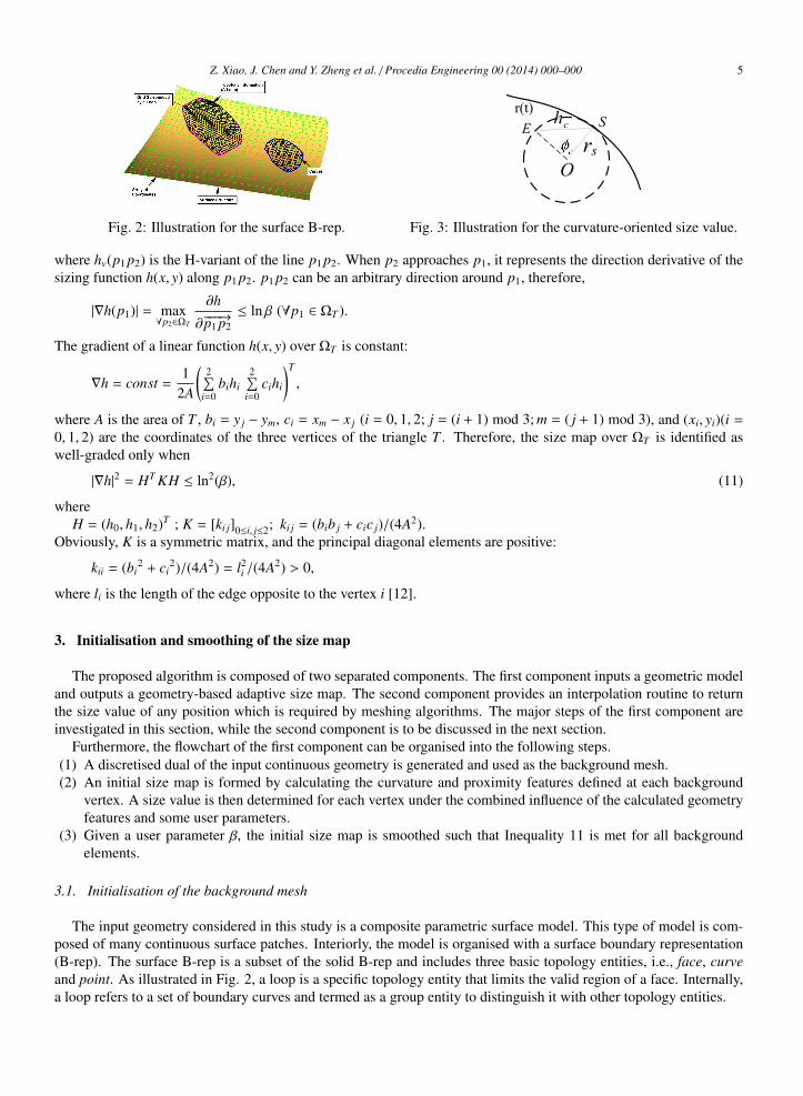
Fig. 2: Illustration for the surface B-rep.

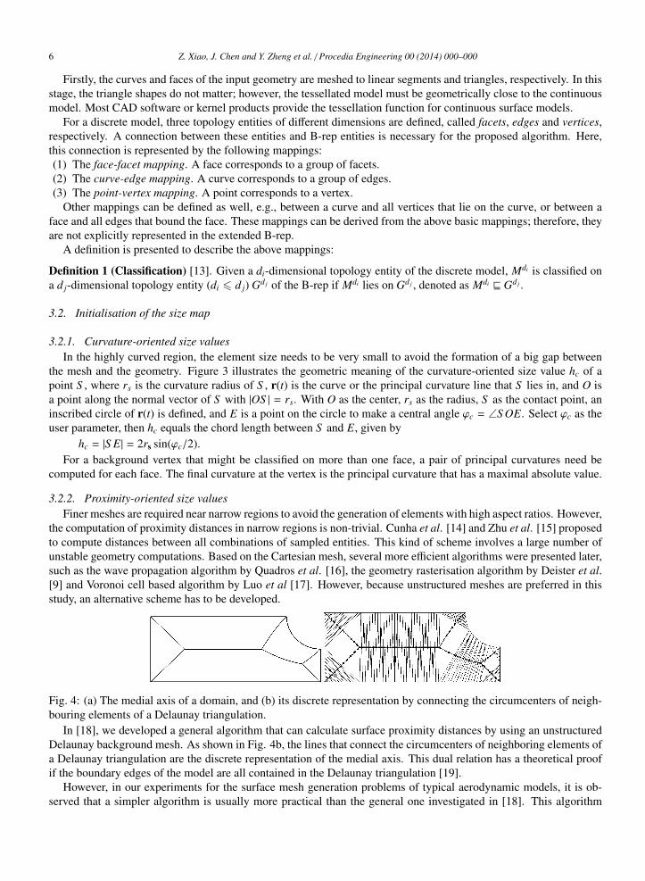
rs

r(t)ch

O

ES

Fig. 3: Illustration for the curvature-oriented size value.

where hv(p1 p2) is the H-variant of the line p1 p2. When p2 approaches p1, it represents the direction derivative of thesizing function h(x, y) along p1 p2. p1 p2 can be an arbitrary direction around p1, therefore,

|∇h(p1)| = max∀p2∈ΩT

∂h

∂−−−→p1 p2≤ ln β (∀p1 ∈ ΩT ).

The gradient of a linear function h(x, y) over ΩT is constant:

∇h = const =1

2A

(2∑

i=0bihi

2∑i=0

cihi

)T

,

where A is the area of T , bi = y j − ym, ci = xm − x j (i = 0, 1, 2; j = (i + 1) mod 3; m = ( j + 1) mod 3), and (xi, yi)(i =

0, 1, 2) are the coordinates of the three vertices of the triangle T . Therefore, the size map over ΩT is identified aswell-graded only when

|∇h|2 = HT KH ≤ ln2(β), (11)

whereH = (h0, h1, h2)T ; K = [ki j]0≤i, j≤2; ki j = (bib j + cic j)/(4A2).

Obviously, K is a symmetric matrix, and the principal diagonal elements are positive:

kii = (bi2 + ci

2)/(4A2) = l2i /(4A2) > 0,

where li is the length of the edge opposite to the vertex i [12].

3. Initialisation and smoothing of the size map

The proposed algorithm is composed of two separated components. The first component inputs a geometric modeland outputs a geometry-based adaptive size map. The second component provides an interpolation routine to returnthe size value of any position which is required by meshing algorithms. The major steps of the first component areinvestigated in this section, while the second component is to be discussed in the next section.

Furthermore, the flowchart of the first component can be organised into the following steps.(1) A discretised dual of the input continuous geometry is generated and used as the background mesh.(2) An initial size map is formed by calculating the curvature and proximity features defined at each background

vertex. A size value is then determined for each vertex under the combined influence of the calculated geometryfeatures and some user parameters.

(3) Given a user parameter β, the initial size map is smoothed such that Inequality 11 is met for all backgroundelements.

3.1. Initialisation of the background mesh

The input geometry considered in this study is a composite parametric surface model. This type of model is com-posed of many continuous surface patches. Interiorly, the model is organised with a surface boundary representation(B-rep). The surface B-rep is a subset of the solid B-rep and includes three basic topology entities, i.e., face, curveand point. As illustrated in Fig. 2, a loop is a specific topology entity that limits the valid region of a face. Internally,a loop refers to a set of boundary curves and termed as a group entity to distinguish it with other topology entities.

6 Z. Xiao, J. Chen and Y. Zheng et al. / Procedia Engineering 00 (2014) 000–000

Firstly, the curves and faces of the input geometry are meshed to linear segments and triangles, respectively. In thisstage, the triangle shapes do not matter; however, the tessellated model must be geometrically close to the continuousmodel. Most CAD software or kernel products provide the tessellation function for continuous surface models.

For a discrete model, three topology entities of different dimensions are defined, called facets, edges and vertices,respectively. A connection between these entities and B-rep entities is necessary for the proposed algorithm. Here,this connection is represented by the following mappings:(1) The face-facet mapping. A face corresponds to a group of facets.(2) The curve-edge mapping. A curve corresponds to a group of edges.(3) The point-vertex mapping. A point corresponds to a vertex.

Other mappings can be defined as well, e.g., between a curve and all vertices that lie on the curve, or between aface and all edges that bound the face. These mappings can be derived from the above basic mappings; therefore, theyare not explicitly represented in the extended B-rep.

A definition is presented to describe the above mappings:

Definition 1 (Classification) [13]. Given a di-dimensional topology entity of the discrete model, Mdi is classified ona d j-dimensional topology entity (di 6 d j) Gd j of the B-rep if Mdi lies on Gd j , denoted as Mdi v Gd j .

3.2. Initialisation of the size map

3.2.1. Curvature-oriented size valuesIn the highly curved region, the element size needs to be very small to avoid the formation of a big gap between

the mesh and the geometry. Figure 3 illustrates the geometric meaning of the curvature-oriented size value hc of apoint S , where rs is the curvature radius of S , r(t) is the curve or the principal curvature line that S lies in, and O isa point along the normal vector of S with |OS | = rs. With O as the center, rs as the radius, S as the contact point, aninscribed circle of r(t) is defined, and E is a point on the circle to make a central angle ϕc = ∠S OE. Select ϕc as theuser parameter, then hc equals the chord length between S and E, given by

hc = |S E| = 2rs sin(ϕc/2).For a background vertex that might be classified on more than one face, a pair of principal curvatures need be

computed for each face. The final curvature at the vertex is the principal curvature that has a maximal absolute value.

3.2.2. Proximity-oriented size valuesFiner meshes are required near narrow regions to avoid the generation of elements with high aspect ratios. However,

the computation of proximity distances in narrow regions is non-trivial. Cunha et al. [14] and Zhu et al. [15] proposedto compute distances between all combinations of sampled entities. This kind of scheme involves a large number ofunstable geometry computations. Based on the Cartesian mesh, several more efficient algorithms were presented later,such as the wave propagation algorithm by Quadros et al. [16], the geometry rasterisation algorithm by Deister et al.[9] and Voronoi cell based algorithm by Luo et al [17]. However, because unstructured meshes are preferred in thisstudy, an alternative scheme has to be developed.

Fig. 4: (a) The medial axis of a domain, and (b) its discrete representation by connecting the circumcenters of neigh-bouring elements of a Delaunay triangulation.

In [18], we developed a general algorithm that can calculate surface proximity distances by using an unstructuredDelaunay background mesh. As shown in Fig. 4b, the lines that connect the circumcenters of neighboring elements ofa Delaunay triangulation are the discrete representation of the medial axis. This dual relation has a theoretical proofif the boundary edges of the model are all contained in the Delaunay triangulation [19].

However, in our experiments for the surface mesh generation problems of typical aerodynamic models, it is ob-served that a simpler algorithm is usually more practical than the general one investigated in [18]. This algorithm

Z. Xiao, J. Chen and Y. Zheng et al. / Procedia Engineering 00 (2014) 000–000 7

computes a global proximity distance for each face:ds = 2.0 × As/ls,

where As is the area of the face and ls is the circumference of the face. For background vertices classified on this face,their proximity-oriented size values are

hd1 = ds/µd,

where the user parameter µd defines the expected number of elements within the proximity distance. Apart from theproximity distance between boundary curves, another proximity feature considered in this study is the curve length,i.e., the distance between the end points of a curve. Because at least one mesh segment is required to be generated in acurve, the size values of a background vertex classified on a curve must be less than the length of the curve. Assumingthat hd0 is the smallest length of all curves containing a background vertex, the final proximity-oriented size value ofthis vertex is

hd = min(hd1, hd0).

3.3. Smoothing of the size map

The initial size map usually disobeys Inequality 11; hence, a smoothing procedure is required to guarantee thatInequality 11 is met for all background triangles. In one of the first solutions to this problem, Borouchaki et al.[11] corrected the size map to ensure that the H-variants of background edges are less than ln β. For a triangle, theH-variants defined on its three edges are only three directional derivatives of the linear sizing function. The fact thattheir values are not greater than ln β is only a necessary condition that requires |∇h| not being greater than ln β. Later,Pippa et al. [12] suggested correcting the size map according to Inequality 11 so that the gradation of the size map islimited everywhere. However, because the smoothing algorithm proposed by Pippa et al. does not attempt to minimisethe change of the size map, its result may deviate a lot from the original size map. Persson et al. [20] formularised theproblem of smoothing a size map to be a Hamilton-Jacobi equation, and many solutions were suggested for differenttypes of background meshes. However, it is doubtful whether this algorithm can be applied in this study becausebackground elements considered here are mainly badly-shaped triangles.

The suggested smoothing algorithm makes a compromise between the algorithm proposed by Borouchaki et al.[11] and that by Persson et al. [12]. Firstly, the background edges are looped to ensure that their H-variants meet therequirement. Assuming that the sets of background mesh vertices and edges are P and E, respectively, the procedurethat smoothes the H-variants of background edges attempts to solve an optimisation problem:

min∑p∈P

(h′(p) − h(p))2

s.t. h′v(e) ≤ ln β(∀e ∈ E)h′(p) ≤ h(p)(∀p ∈ P)

, (12)

where h′v(e) is the H-variant of a mesh edge e after smoothing. Note that the one-way adjustment only reduces the sizevalues of background vertices. By solving this optimisation problem, the change to the original size map is minimisedby a least square method. There are many standard solutions for this optimisation problem. In our implementation, theopen-sourced code LPSolve [21] is employed. In practice, only a very small fraction of background elements disobeyInequality 11 after the first stage of smoothing. The background elements that disobey Inequality 11 are put into anarray, and for each of them, a correction scheme is executed [12]. Note that the background triangles are defined inthree dimensions. Each triangle must be transformed to a new coordinate system that uses the normal vector of thetriangle as the Z axis before conducting the correction scheme depicted as below:

(1) Assuming that h0 ≤ h1 ≤ h2, the value of h2 is altered such that |∇h|2 = ln2(β):

h′2 = (−rb +

√r2

b − 4rarc)/(2ra),

wherera = k22

rb = (k02 + k20)h0 + (k21 + k12)h1 = 2k02h0 + 2k12h1

rc = k00h20 + (k01 + k10)h0h1 + k11h2

1 − ln2(β) = k00h20 + 2k01h0h1 + k11h2

1 − ln2(β)

.

8 Z. Xiao, J. Chen and Y. Zheng et al. / Procedia Engineering 00 (2014) 000–000

(2) Obviously, h′2 does not have a real value when r2b − 4rarc < 0. In this case, we attempt to alter the values of h1

and h2 simultaneously such that

h′1 = h′2 = (−zb +

√z2

b − 4zazc)/(2za),where

za = k11 + k12 + k21 + k22 = k11 + 2k12 + k22 = −(k01 + k02) = k00

zb = (k01 + k10 + k02 + k20)h0 = 2(k01 + k02)h0 = 2k00h0

zc = k00h20 − ln2(β)

.

h′1 and h′2 always have a real value sincez2

b − 4zazc = 4k200h2

0 − 4k00(k00h20 − ln2(β)) = 4k00ln2(β) ≥ 0.

3.4. User options

An element-sizing specification algorithm attempts to reduce the intensity of user interactions because manualspecification of the sizing information is tedious and time-consuming. However, the user priori expertise for thesimulation problem is usually very important for preparing a suitable mesh model. Its role is currently irreplaceable inmany meshing tasks. Therefore, the proposed algorithm provides the user with options to influence the element-sizingresults via the following parameters so that a variety of meshes can be generated to satisfy different simulation needs:(1) Global user parameters ϕc, µd and β. (2) A local ϕc value for any curve or face. (3) Local µd and β values for anyface. (4) A predefined size value or function for any geometry point, curve or face.

Only the first group of parameters is mandatory and the other parameters are optional. In most meshing tasks, theuser need only set the mandatory parameters. For each background vertex, its initial size value is computed under thecombined influence of the calculated geometry features and user parameters:

ha = max(hmin,min(hd, hc, hu, hmax)),where hc and hd are curvature and proximity oriented size values, respectively; hu is the predefined size value by theuser (if any); and hmin and hmax are the user parameters which limit the minimal and maximal size values.

4. Integration scheme with a surface mesher

Once the size map defined on the background mesh is smoothed, it is ready to provide the interpolation servicefor mesh generation algorithms. In its simplest form, the interpolation routine inputs the coordinates of a point, thenreturns the size value defined on that point. Interiorly, this routine takes two steps:(1) Search for the background element that contains the point (referred to as a base element hereafter);(2) Interpolate the size value of this point with the size values of the forming vertices of the base element.

The efficiency of the first step heavily impacts the efficiency of the meshing procedure. Taking a sequential advanc-ing front surface mesher as the example, we will introduce how the proposed algorithm can serve a typical surfacemesher efficiently.

4.1. The sequential surface mesher

Like most of prevailing surface meshers, our mesher exploits the parametric representation of input surfaces, andcan be classified as mapping based. In contrast, some authors suggested generating the mesh in the original physicalspace [22–24], and the algorithms they adopt are referred to as direct algorithms. Mapping based algorithms can adoptthe advancing front technique (AFT) [22–25], Delaunay triangulation [26,27] or a combination of two techniques [28]to mesh the parametric region of a surface. To handle the mapping distortion, the parametric region is covered by aRiemannian metric [26,27] or a normalised matrix [25], where the length of an ideal mesh edge is always one. Inthe CFD community, the advancing front surface mesher is favored because it provides better control on the elementshapes, in particular in the neighborhood of surface boundaries. However, with respect to the timing performance, aDelaunay mesher may run faster by several times than an advancing front mesher.

The surface models used in the real world may be badly parameterized. If no cautions are taken, an advancing frontmesher may fail to handle these surfaces, or even if succeed, provide invalid or badly shaped elements. To enhancethe robustness, Tremel et al. suggested two procedures [29]:

Z. Xiao, J. Chen and Y. Zheng et al. / Procedia Engineering 00 (2014) 000–000 9

(1) Calculate the ideal point of a given front in the physical space instead of the parametric space.(2) Check the validity of a new element in the physical space instead of the parametric space.

As demonstrated by Tremel et al., these two procedures improve the robustness of their mesher up to a productionlevel. However, it is observed that the two procedures defined in the physical space are time consuming and do slowdown their surface mesher [29].

The advancing front mesher adopted in this study is enhanced with the above two procedures as well. In ourtests, the procedure that calculates ideal points in the physical space mainly accounts for the slowdown of the surfacemesher. To improve the timing performance but not to sacrifice the robustness, we choose to employ this procedureadaptively. In our implementation, the more efficient procedure that calculates ideal points in the parametric space isemployed in default, and the improved procedure is employed only when the outcome of the default procedure is notsatisfactory.

4.2. The base-element search routine

For a Cartesian background mesh, the time complexity of the base-element search routine is proportional to thedepth of the tree that stores the mesh. However, for an unstructured background mesh, a brute-force search procedureconsumes O(n) time in its worst case, where n is the number of background elements required to be searched. In amesh generation process, the number of callings for this search routine is several times of the number of mesh nodesto be generated. Therefore, a fast base-element search routine is mandatory.

Because the surface mesher deals with faces individually in parametric spaces, the search routine can be imple-mented in the two-dimensional parametric space of a face as well. Apart from physical coordinates, each backgroundvertex stores the parametric coordinates in its classification faces. When the surface mesher queries the size value ofa point, it inputs the face ID and the parametric coordinates of the point. The base-element search procedure onlyvisits the background elements classified on the input face, and moreover, the search occurs in the two-dimensionalparametric space of the input face instead of the three-dimensional physical space.

The timing performance of the search routine can be further improved if we make the most of the spatial locality ofthe searching callings, i.e., the base elements for two close positions are usually similar or adjacent. A smarter searchprocedure can be developed by inputting one more parameter that refers to a good enough guess for the base element.In our algorithm, the procedure suggested by Shan et al. is adopted [30], which requires no auxiliary structures butthe initial guess and neighboring indices of background elements.

For an advancing front algorithm, a front is first selected, and a new node is then created. Obviously, when queryingthe base element of the new node, either of the base elements of the front nodes can be chosen as the initial guess.

5. Results

The proposed algorithm has been integrated into an in-house preprocessor HEDP/Pre developed at our lab [31]. Todemonstrate the capabilities of the proposed algorithm, we select two aircraft models: the F6 model [32] and the F16fighting aircraft (referred to as F16 hereafter). All the tests presented here were conducted on a PC (CPU: 3.5GHz,Memory: 24GB).

5.1. F6 aircraft model

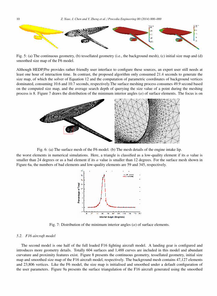
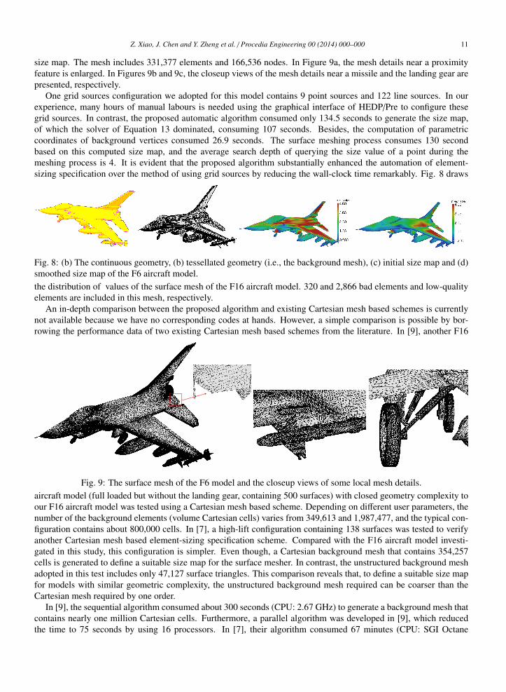
The F6 model contains 35 surfaces and 97 curves. Figure 5 presents its continuous geometry, tessellated geometry(i.e., the background mesh), initial size map and smoothed size map, respectively. The background mesh contains14,406 elements and 7,312 vertices. The size map is initialised and smoothed by using the default user parameters:ϕc = 5; µd = 2; β = 1.2. Figure 6 presents the surface triangulation generated using the smoothed size map.The mesh includes 113,385 elements and 56,968 nodes. Figure 6b shows the mesh details of the engine intake lipin a strongly magnified resolution. A very fine mesh resolution is observed in the engine intake lip because highcurvature features exist there. Moreover, the variation of element scales is controlled very well owing to the proposedsmoothing procedure for the size map. We used to configure grid sources to define the size map of this model before.One configuration we adopted frequently for exterior flow simulations includes 31 line sources and 3 point sources.

10 Z. Xiao, J. Chen and Y. Zheng et al. / Procedia Engineering 00 (2014) 000–000

Fig. 5: (a) The continuous geometry, (b) tessellated geometry (i.e., the background mesh), (c) initial size map and (d)smoothed size map of the F6 model.

Although HEDP/Pre provides rather friendly user interface to configure these sources, an expert user still needs atleast one hour of interaction time. In contrast, the proposed algorithm only consumed 21.4 seconds to generate thesize map, of which the solver of Equation 12 and the computation of parametric coordinates of background verticesdominated, consuming 10.6 and 10.7 seconds, respectively.The surface meshing process consumes 49.9 second basedon the computed size map, and the average search depth of querying the size value of a point during the meshingprocess is 8. Figure 7 draws the distribution of the minimum interior angles (α) of surface elements. The focus is on

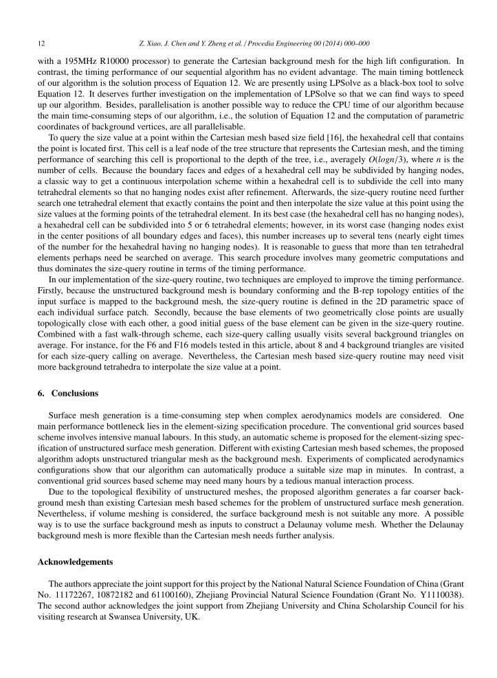
Fig. 6: (a) The surface mesh of the F6 model. (b) The mesh details of the engine intake lip.the worst elements in numerical simulations. Here, a triangle is classified as a low-quality element if its α value issmaller than 24 degrees or as a bad element if its α value is smaller than 12 degrees. For the surface mesh shown inFigure 6a, the numbers of bad elements and low-quality elements are 59 and 345, respectively.

Fig. 7: Distribution of the minimum interior angles (α) of surface elements.

5.2. F16 aircraft model

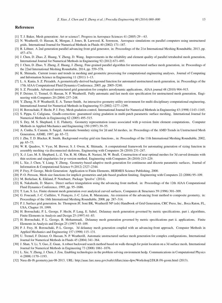
The second model is one half of the full loaded F16 fighting aircraft model. A landing gear is configured andintroduces more geometry details. Totally 604 surfaces and 1,488 curves are included in this model and abundantcurvature and proximity features exist. Figure 8 presents the continuous geometry, tessellated geometry, initial sizemap and smoothed size map of the F16 aircraft model, respectively. The background mesh contains 47,127 elementsand 23,806 vertices. Like the F6 model, the size map is initialised and smoothed under a default configuration ofthe user parameters. Figure 9a presents the surface triangulation of the F16 aircraft generated using the smoothed

Z. Xiao, J. Chen and Y. Zheng et al. / Procedia Engineering 00 (2014) 000–000 11

size map. The mesh includes 331,377 elements and 166,536 nodes. In Figure 9a, the mesh details near a proximityfeature is enlarged. In Figures 9b and 9c, the closeup views of the mesh details near a missile and the landing gear arepresented, respectively.

One grid sources configuration we adopted for this model contains 9 point sources and 122 line sources. In ourexperience, many hours of manual labours is needed using the graphical interface of HEDP/Pre to configure thesegrid sources. In contrast, the proposed automatic algorithm consumed only 134.5 seconds to generate the size map,of which the solver of Equation 13 dominated, consuming 107 seconds. Besides, the computation of parametriccoordinates of background vertices consumed 26.9 seconds. The surface meshing process consumes 130 secondbased on this computed size map, and the average search depth of querying the size value of a point during themeshing process is 4. It is evident that the proposed algorithm substantially enhanced the automation of element-sizing specification over the method of using grid sources by reducing the wall-clock time remarkably. Fig. 8 draws

Fig. 8: (b) The continuous geometry, (b) tessellated geometry (i.e., the background mesh), (c) initial size map and (d)smoothed size map of the F6 aircraft model.the distribution of values of the surface mesh of the F16 aircraft model. 320 and 2,866 bad elements and low-qualityelements are included in this mesh, respectively.

An in-depth comparison between the proposed algorithm and existing Cartesian mesh based schemes is currentlynot available because we have no corresponding codes at hands. However, a simple comparison is possible by bor-rowing the performance data of two existing Cartesian mesh based schemes from the literature. In [9], another F16

Fig. 9: The surface mesh of the F6 model and the closeup views of some local mesh details.aircraft model (full loaded but without the landing gear, containing 500 surfaces) with closed geometry complexity toour F16 aircraft model was tested using a Cartesian mesh based scheme. Depending on different user parameters, thenumber of the background elements (volume Cartesian cells) varies from 349,613 and 1,987,477, and the typical con-figuration contains about 800,000 cells. In [7], a high-lift configuration containing 138 surfaces was tested to verifyanother Cartesian mesh based element-sizing specification scheme. Compared with the F16 aircraft model investi-gated in this study, this configuration is simpler. Even though, a Cartesian background mesh that contains 354,257cells is generated to define a suitable size map for the surface mesher. In contrast, the unstructured background meshadopted in this test includes only 47,127 surface triangles. This comparison reveals that, to define a suitable size mapfor models with similar geometric complexity, the unstructured background mesh required can be coarser than theCartesian mesh required by one order.

In [9], the sequential algorithm consumed about 300 seconds (CPU: 2.67 GHz) to generate a background mesh thatcontains nearly one million Cartesian cells. Furthermore, a parallel algorithm was developed in [9], which reducedthe time to 75 seconds by using 16 processors. In [7], their algorithm consumed 67 minutes (CPU: SGI Octane

12 Z. Xiao, J. Chen and Y. Zheng et al. / Procedia Engineering 00 (2014) 000–000

with a 195MHz R10000 processor) to generate the Cartesian background mesh for the high lift configuration. Incontrast, the timing performance of our sequential algorithm has no evident advantage. The main timing bottleneckof our algorithm is the solution process of Equation 12. We are presently using LPSolve as a black-box tool to solveEquation 12. It deserves further investigation on the implementation of LPSolve so that we can find ways to speedup our algorithm. Besides, parallelisation is another possible way to reduce the CPU time of our algorithm becausethe main time-consuming steps of our algorithm, i.e., the solution of Equation 12 and the computation of parametriccoordinates of background vertices, are all parallelisable.

To query the size value at a point within the Cartesian mesh based size field [16], the hexahedral cell that containsthe point is located first. This cell is a leaf node of the tree structure that represents the Cartesian mesh, and the timingperformance of searching this cell is proportional to the depth of the tree, i.e., averagely O(logn/3), where n is thenumber of cells. Because the boundary faces and edges of a hexahedral cell may be subdivided by hanging nodes,a classic way to get a continuous interpolation scheme within a hexahedral cell is to subdivide the cell into manytetrahedral elements so that no hanging nodes exist after refinement. Afterwards, the size-query routine need furthersearch one tetrahedral element that exactly contains the point and then interpolate the size value at this point using thesize values at the forming points of the tetrahedral element. In its best case (the hexahedral cell has no hanging nodes),a hexahedral cell can be subdivided into 5 or 6 tetrahedral elements; however, in its worst case (hanging nodes existin the center positions of all boundary edges and faces), this number increases up to several tens (nearly eight timesof the number for the hexahedral having no hanging nodes). It is reasonable to guess that more than ten tetrahedralelements perhaps need be searched on average. This search procedure involves many geometric computations andthus dominates the size-query routine in terms of the timing performance.

In our implementation of the size-query routine, two techniques are employed to improve the timing performance.Firstly, because the unstructured background mesh is boundary conforming and the B-rep topology entities of theinput surface is mapped to the background mesh, the size-query routine is defined in the 2D parametric space ofeach individual surface patch. Secondly, because the base elements of two geometrically close points are usuallytopologically close with each other, a good initial guess of the base element can be given in the size-query routine.Combined with a fast walk-through scheme, each size-query calling usually visits several background triangles onaverage. For instance, for the F6 and F16 models tested in this article, about 8 and 4 background triangles are visitedfor each size-query calling on average. Nevertheless, the Cartesian mesh based size-query routine may need visitmore background tetrahedra to interpolate the size value at a point.

6. Conclusions

Surface mesh generation is a time-consuming step when complex aerodynamics models are considered. Onemain performance bottleneck lies in the element-sizing specification procedure. The conventional grid sources basedscheme involves intensive manual labours. In this study, an automatic scheme is proposed for the element-sizing spec-ification of unstructured surface mesh generation. Different with existing Cartesian mesh based schemes, the proposedalgorithm adopts unstructured triangular mesh as the background mesh. Experiments of complicated aerodynamicsconfigurations show that our algorithm can automatically produce a suitable size map in minutes. In contrast, aconventional grid sources based scheme may need many hours by a tedious manual interaction process.

Due to the topological flexibility of unstructured meshes, the proposed algorithm generates a far coarser back-ground mesh than existing Cartesian mesh based schemes for the problem of unstructured surface mesh generation.Nevertheless, if volume meshing is considered, the surface background mesh is not suitable any more. A possibleway is to use the surface background mesh as inputs to construct a Delaunay volume mesh. Whether the Delaunaybackground mesh is more flexible than the Cartesian mesh needs further analysis.

Acknowledgements

The authors appreciate the joint support for this project by the National Natural Science Foundation of China (GrantNo. 11172267, 10872182 and 61100160), Zhejiang Provincial Natural Science Foundation (Grant No. Y1110038).The second author acknowledges the joint support from Zhejiang University and China Scholarship Council for hisvisiting research at Swansea University, UK.

Z. Xiao, J. Chen and Y. Zheng et al. / Procedia Engineering 00 (2014) 000–000 13

References

[1] T. J. Baker, Mesh generation: Art or science?, Progress in Aerospace Sciences 41 (2005) 29 – 63.[2] N. Weatherill, O. Hassan, K. Morgan, J. Jones, B. Larwood, K. Sorenson, Aerospace simulations on parallel computers using unstructured

grids, International Journal for Numerical Methods in Fluids 40 (2002) 171–187.[3] R. Lohner, A 2nd generation parallel advancing front grid generator, in: Proceedings of the 21st International Meshing Roundtable, 2013, pp.

457–474.[4] J. Chen, D. Zhao, Z. Huang, Y. Zheng, D. Wang, Improvements in the reliability and element quality of parallel tetrahedral mesh generation,

International Journal for Numerical Methods in Engineering 92 (2012) 671–693.[5] J. Chen, D. Zhao, Y. Zheng, Z. Huang, J. Zheng, Fine-grained parallel algorithm for unstructured surface mesh generation, in: Proceedings of

the 22nd International Meshing Roundtable, 2014, pp. 559–578.[6] K. Shimada, Current issues and trends in meshing and geometric processing for computational engineering analyses, Journal of Computing

and Information Science in Engineering 11 (2011) 1–13.[7] L. A. Kania, S. Z. Pirzadeh, A geometrically-derived background function for automated unstructured mesh generation, in: Proceedings of the

17th AIAA Computational Fluid Dynamics Conference, 2005, pp. 2005–5240.[8] S. Z. Pirzadeh, Advanced unstructured grid generation for complex aerodynamic applications, AIAA journal 48 (2010) 904–915.[9] F. Deister, U. Tremel, O. Hassan, N. P. Weatherill, Fully automatic and fast mesh size specification for unstructured mesh generation, Engi-

neering with Computers 20 (2004) 237–248.[10] Y. Zheng, N. P. Weatherill, E. A. Turner-Smith, An interactive geometry utility environment for multi-disciplinary computational engineering,

International Journal for Numerical Methods in Engineering 53 (2002) 1277–1299.[11] H. Borouchaki, F. Hecht, P. J. Frey, Mesh gradation control, International Journal for Numerical Methods in Engineering 43 (1998) 1143–1165.[12] S. Pippa, G. Caligiana, Gradh-correction: guaranteed sizing gradation in multi-patch parametric surface meshing, International Journal for

Numerical Methods in Engineering 62 (2005) 495–515.[13] S. Dey, M. S. Shephard, J. E. Flaherty, Geometry representation issues associated with p-version finite element computations, Computer

Methods in Applied Mechanics and Engineering 150 (1997) 39–55.[14] A. Cunha, S. Canann, S. Saigal, Automatic boundary sizing for 2d and 3d meshes, in: Proceedings of the AMD Trends in Unstructured Mesh

Generation, ASME, 1997, pp. 65–72.[15] J. Zhu, T. D. Blacker, R. Smith, Background overlay grid size functions., in: Proceedings of the 11th International Meshing Roundtable, 2002,

pp. 65–73.[16] W. R. Quadros, V. Vyas, M. Brewer, S. J. Owen, K. Shimada, A computational framework for automating generation of sizing function in

assembly meshing via disconnected skeletons, Engineering with Computers 26 (2010) 231–247.[17] X.-J. Luo, M. S. Shephard, L.-Z. Yin, R. M. OBara, R. Nastasi, M. W. Beall, Construction of near optimal meshes for 3d curved domains with

thin sections and singularities for p-version method, Engineering with Computers 26 (2010) 215–229.[18] L. Xie, J. Chen, Y. Liang, Y. Zheng, Geometry-based adaptive mesh generation for continuous and discrete parametric surfaces, Journal of

Information & Computational Science 9 (2012) 2327–2344.[19] P. Frey, P. George, Mesh Generation: Application to Finite Elements, HERMES Science Publishing, 2000.[20] P.-O. Persson, Mesh size functions for implicit geometries and pde-based gradient limiting, Engineering with Computers 22 (2006) 95–109.[21] M. Berkelaar, K. Eikland, P. Notebaert, Package ’lpsolve’ (2014).[22] K. Nakahashi, D. Sharov, Direct surface triangulation using the advancing front method, in: Proceedings of the 12th AIAA Computational

Fluid Dynamics Conference, 1995, pp. 95–1686.[23] T. Lan, S. Lo, Finite element mesh generation over analytical curved surfaces, Computers & Structures 59 (1996) 301–309.[24] G. Foucault, J.-C. Cuilliere, V. Francois, J.-C. Leon, R. Maranzana, An extension of the advancing front method to composite geometry, in:

Proceedings of the 16th International Meshing Roundtable, 2008, pp. 287–314.[25] P. J, Surface grid generation. In: Thompson JF, Soni BK, Weatherill NP (eds) Handbook of Grid Generation, CRC Press, Inc., Boca Raton, FL,

USA, Chapter 19, 1999.[26] H. Borouchaki, P. L. George, F. Hecht, P. Laug, E. Saltel, Delaunay mesh generation governed by metric specifications. part i. algorithms,

Finite Elements in Analysis and Design 25 (1997) 61–83.[27] H. Borouchaki, P. L. George, B. Mohammadi, Delaunay mesh generation governed by metric specifications part ii. applications, Finite

Elements in Analysis and Design 25 (1997) 85–109.[28] P. J. Frey, H. Borouchaki, P.-L. George, 3d delaunay mesh generation coupled with an advancing-front approach, Computer Methods in

Applied Mechanics and Engineering 157 (1998) 115–131.[29] U. Tremel, F. Deister, O. Hassan, N. P. Weatherill, Automatic unstructured surface mesh generation for complex configurations, International

Journal for Numerical Methods in Fluids 45 (2004) 341–364.[30] J. Shan, Y. Li, Y. Guo, Z. Guan, A robust backward search method based on walk-through for point location on a 3d surface mesh, International

Journal for Numerical Methods in Engineering 73 (2008) 1061–1076.[31] L. Xie, Y. Zheng, J. Chen, J. Zou, Enabling technologies in the problem solving environment hedp, Communications in Computational Physics

4 (2008) 1170–1193.[32] Nasa dlr-f6 geometry.jun-08-2013, URL: http://aaac.larc.nasa.gov/tsab/cfdlarc/aiaa-dpw/Workshop2/DLR-F6-geom.html (2013).