Master Thesis

Wireless LoudspeakerSystem With Real-Time

Audio CompressionAuthor: Ivar LoekkenEmployer: Chipcon ASUniversity: Norwegian University of Technology and Science (NTNU)Instructor: Robin Osa Hoel, ChipconLanguage: EnglishNumber of pages: 240 including appendixes.

Abstract: Hardware for a fully digital wireless loudspeaker system basedaround the Chipcon CC2400 RF-transceiver has been designed.Research on suitable low-complexity compression algorithms isdocumented. This includes both lossy and losslesscompression. In both cases, algorithm suggestions have beenmade based on measurements, complexity estimations andlistening tests. A lossy algorithm, iLaw, is presented, whichimproves µ-law encoding to provide audio quality comparableto MP3. A lossless algorithm is suggested, which features alossy-mode to provide constant bitrate with minimal qualitydegradation. The algorithm is based around Pod-coding, ascheme not previously used in any compression software. Pod-coding is simple, efficient and has properties that are veryadvantageous in a real-time application.

Keywords: Audio compression, low-complexity, lossless, lossy, Pod-encoding, Rice-encoding, µ-law, ADPCM, wirelessloudspeaker

Ivar Loekken, 28/5-2004.

1

2

Introduction

This thesis will cover the work done developing a system for wireless audiotransmission. The intended application is a wireless loudspeaker system1 where a hificontrol and playback unit transmits data to remote active speakers using an RFtranceiver.

This concept is not new, but while most such systems use analog FM transfer, whichwill inevitably compromise audio quality, the transmission in this WLS will be fullydigital with AD-conversion in the transmitter and DA-conversion in the receiver. Adigital input will also be available. The transmission will be done using a ChipconCC2400 RF-transceiver with 1Mbps transfer rate. Chipcon, who is the employer forthis project, intends to use the WLS as a demonstration or reference design for theCC2400.

The informed reader might notice that the 1Mbps transfer rate is insufficient for CD-quality audio, which requires about 1.4Mbps. This will be resolved using real-timecompression. The main focus of the thesis work has been on developing a low-complexity and high-quality compression algorithm that can be run using only asimple MCU. The employer required the design to be low-cost so separate DSPs orASICs for compression was not an option. Both lossless and lossy algorithms havebeen explored2.

Originally, development was intended to be done using a MCU evaluation board.However, none of these had the necessary peripherals. Design of the reference systemwas thus included as a part of the thesis. This led to some delays, and also themanufacturing of the PCB (done by Chipcon) was significantly delayed3. Because ofthis, a full implementation in hardware was not achieved before the thesis deadline.But although implementation is an important task, this has not had any significanteffect on the thesis itself. As mentioned the academical focus was on developing asuitable compression scheme, and both a custom lossless and lossy algorithm hasbeen suggested. These algorithms have been tested and documented by writing andcompliling them on a computer4 and running them on waveform audio files.

The thesis is divided into two main parts. The first covers audio compression theoryand gives the reader the basis knowledge necessary to understand how the algorithmswork. The second part covers the deveopement itself and provides documentation ofthe work done. This includes both hardware and software design. Finally, the project

1 Througout the thesis, the target application will be referred to as the Wireless Louspeaker System orsimply the WLS.2 A lossless compression algorithm is one where the output after decompression is identical to theoriginal data. In lossy algorithms, psychoacoustic models are used to remove audio information that isnot perceptible.3 This is detailed in the project review, included at the end of the thesis.4 Apple Powerbook G4 running Mac OS-X 10.3 ”Panther”.

3

itself is reviewed and a discussion around the work process, the achievements made aswell as the academical rewards is presented.

Finally I’d like to thank the following persons who have been of great help during theproject:

- Robin Osa Hoel, my supervisor at Chipcon, for giving of his time toanswer questions, review my work and provide general guidance througoutthe project.

- Albert Wegener of Soundspace Audio for providing an evaluation licenseof his algorithm MusiCompress for study, and also for patiently answeringquestions I’ve had regarding audio compression.

- Tore Barlindhaug, engineer at NTNU, for lending me a computer monitorthe entire semester, so I was releived from the ergonomical strain ofstaring at a small laptop display ten hours a day.

4

Table of Contents

1 Wireless Loudspeaker System Description ......................................................112 Audio Compression; Theory and Principles ....................................................13

2.1 An information-based approach to digital audio...................................................132.2 Lossless compression of audio..................................................................................16

2.2.1 Framing................................................................................................................................. 162.2.2 Decorrelation ........................................................................................................................ 17

2.2.2.1 Inter-channel decorrelation ........................................................................................ 172.2.2.2 Intra-channel decorrelation ........................................................................................ 18

2.2.2.2.1 Linear prediction................................................................................................... 202.2.2.2.2 Adaptive prediction .............................................................................................. 232.2.2.2.3 Polyonimal approximation ................................................................................... 24

2.2.3 Entropy-coding..................................................................................................................... 262.2.3.1 Run-length encoding (RLE)....................................................................................... 262.2.3.2 Huffman-coding ......................................................................................................... 262.2.3.3 Adaptive Huffman coding.......................................................................................... 302.2.3.4 Rice-coding................................................................................................................. 33

2.2.3.4.1 Calculating the parameter k .................................................................................. 342.2.3.5 Pod-coding, a better way to code the overflow......................................................... 36

2.3 Lossy compression of audio ......................................................................................372.3.1 The human auditory system................................................................................................. 372.3.2 Lossy compression algorithms ............................................................................................ 41

2.3.2.1 MPEG-based algorithms............................................................................................ 422.3.2.2 Differential Pulse Code Modulation (DPCM) .......................................................... 442.3.2.3 Adaptive DPCM (ADPCM)....................................................................................... 45

2.3.2.3.1 IMA ADPCM adaptive quantizer ........................................................................ 462.3.2.4 µ-Law.......................................................................................................................... 49

3 Hardware Design.............................................................................................533.1 Selection of components ............................................................................................53

3.1.1 RF-transceiver: the Chipcon SmartRF! CC2400................................................................ 543.1.2 Audio codec.......................................................................................................................... 553.1.3 SP-dif receiver...................................................................................................................... 573.1.4 Selection of microcontroller ................................................................................................ 59

3.1.4.1 Speed requirements .................................................................................................... 593.1.4.2 Memory requirements ................................................................................................ 603.1.4.3 I/O requirements......................................................................................................... 613.1.4.4 Evaluated microcontrollers ........................................................................................ 62

3.1.4.4.1 Atmel AVR Mega169L and Mega32L ................................................................ 633.1.4.4.2 Texas Instruments MSP430F1481 ....................................................................... 643.1.4.4.3 Motorola DSP56F801........................................................................................... 653.1.4.4.4 Hitachi/Rensas R8C/10 Tiny................................................................................ 663.1.4.4.5 Silicon Laboratories C8051F005 ......................................................................... 67

3.1.5 Conclusions: ......................................................................................................................... 68

3.2 Audio transfer to MCU .............................................................................................693.2.1 Principle for data transfer, audio device - MCU................................................................. 693.2.2 Realization of data transfer, audio device - MCU .............................................................. 70

3.2.2.1 Serial-to-parallell and parallell-to-serial conversion ................................................ 703.2.2.2 Design of logic to create necessary control signals .................................................. 73

3.3 Circuit design .............................................................................................................753.3.1 Configuration of the SP-dif receiver. .................................................................................. 763.3.2 Configuration of the audio codec ........................................................................................ 77

5

3.3.3 Configuration of the RF-transceiver.................................................................................... 793.3.4 Configuration of the MCU IO ............................................................................................. 803.3.5 The finished circuit .............................................................................................................. 83

4 Analysis of Lossy Compression Algorithms.....................................................864.1 Reference for comparison; 8-bit and 4-bit LPCM ................................................874.2 Analysis of 4-bit DPCM ............................................................................................884.3 Analysis of IMA ADPCM .........................................................................................904.4 Analysis of µ-law........................................................................................................914.5 Reference for comparison II: MP3..........................................................................934.6 iLaw: a low-complexity, low-loss algorithm...........................................................964.7 Notes about the performance measurements .........................................................99

5 Design of Lossless Compression Algorithm...................................................1005.1 Coding method .........................................................................................................103

5.1.1 Evaluation of Pod-coding and Rice-coding ...................................................................... 103

5.2 iPod: an attempt at improving the Pod-coding....................................................1075.3 Prediction scheme ....................................................................................................1105.4 Channel decorrelation.............................................................................................1155.5 Final algorithm proposal and benchmark............................................................1195.6 Lossy mode................................................................................................................121

5.6.1 LSB-removal lossy-mode .................................................................................................. 1225.6.2 Mono samples lossy-mode................................................................................................. 125

6 WLS Implementation Considerations............................................................1276.1 MCU implementation considerations....................................................................127

6.1.1 Wrap-around arithmetic ..................................................................................................... 1276.1.2 Look-up tables.................................................................................................................... 128

6.2 RF-link implementation considerations................................................................1296.2.1 Packet handling .................................................................................................................. 1296.2.2 Transmission or calculation of k ?..................................................................................... 1306.2.3 Lost packet handling .......................................................................................................... 130

7 Project Review ...............................................................................................1358 Summary .......................................................................................................1369 References .....................................................................................................137

Appendix 1 Data Formats _________________________________________142Appendix 2 Data Converter Fundamentals____________________________148Appendix 3 Schematics____________________________________________155Appendix 4 Components List_______________________________________162Appendix 5 PCB- Layout__________________________________________163Appendix 6 Souce-Code C_________________________________________176Appendix 7 Matlab-Scripts ________________________________________235Appendix 8 Tools Used During Development__________________________239

6

List of Figures

Figure 1 Wireless loudpeaker system........................................................................................................... 12Figure 2 Digital representation of audio signal............................................................................................ 13Figure 3 Histogram of samples in Stevie Ray Vaughan, ”Voodoo Chile” wav-file .................................. 15Figure 4 Basic principles of lossless audio compression............................................................................. 16Figure 5 Histogram of mutual and side, "Voodoo Chile", 30s excerpt....................................................... 18Figure 6 Prediction model [reference 2]....................................................................................................... 19Figure 7 Histogram, prediction error e[n], "Voodoo Chile", 30s excerpt................................................... 20Figure 8 Signal flow chart, difference prediction ........................................................................................ 21Figure 9 General filter-based prediction [reference 2] ................................................................................ 21Figure 10 Entropy vs. predictor order, fixed FIR predictor........................................................................ 23Figure 11 The four polynomal approximations of x[n] [reference 2] ......................................................... 25Figure 12 Binary tree with prefix property code (code 2 from table 3)...................................................... 28Figure 13 General depiction of Huffman-tree, seven symbols W1-W7 ..................................................... 29Figure 14 Algorithm FGK processing the ensemble EX: (a) Tree after processing "aa bb"; 11 will be

transmitted for the next b. (b) After encoding the third b; 101 will be transmitted for the nextspace; the tree will not change; 100 will be transmitted for the first c. (c) Tree after updatefollowing first c. [reference 9] ............................................................................................................ 31

Figure 15 Complete Huffman-tree for example EX .................................................................................... 32Figure 16 The human auditory system......................................................................................................... 37Figure 17 Cross-section of the cochlea ........................................................................................................ 38Figure 18 Cochlea filter response................................................................................................................. 39Figure 19 Masking threshold ........................................................................................................................ 39Figure 20 The Fletcher-Munson curves (equal loudness curves)................................................................ 40Figure 21 Temporal masking........................................................................................................................ 41Figure 22 MP3 encoding and decoding block diagram ............................................................................... 42Figure 23 AAC compression block diagram................................................................................................ 43Figure 24 DPCM-encoder block diagram [reference 17] ............................................................................ 44Figure 25 DPCM decoder block diagram [reference 17] ............................................................................ 45Figure 26 ADPCM general block diagram [referene 18] ............................................................................ 46Figure 27 IMA ADPCM stepsize adaptation [reference 18]....................................................................... 47Figure 28 IMA ADPCM quantization [reference 18].................................................................................. 48Figure 29 Basic block diagram, wireless audio transceiver ........................................................................ 53Figure 30 Typical application circuit, Chipcon CC2400 [reference 22]..................................................... 54Figure 31 Texas Instruments TLV320AIC23B block diagram [reference 24] ........................................... 56Figure 32 Block diagram, Crystal CS8416 [reference 28] .......................................................................... 58Figure 33 Communication through a) 2 SPI-ports or b) 1 SPI-port and parallell IO via shift registers.... 61Figure 34 I2S data transfer timing diagram .................................................................................................. 69Figure 35 Principle for data transfer between audio device and MCU....................................................... 70Figure 36 Simplified schematics, 74HC4094N [reference 37] ................................................................... 71Figure 37 Tming diagram, transfer from audio device to MCU ................................................................. 71Figure 38 Logic diagram, 74HC166N [reference 38].................................................................................. 72Figure 39 Timing diagram, transfer from MCU to audio device ................................................................ 72Figure 40 Logic circuit for generation of control signals ............................................................................ 73Figure 41 Timing diagram for control signals ............................................................................................. 74Figure 42 Block diagram, wireless loudspeaker system............................................................................. 75Figure 43 Configuration of SP-dif receiver.................................................................................................. 76Figure 44 Recommended filter layout [reference 27].................................................................................. 77Figure 45 220µF, 330µF, 470µF decoupling caps frequency response, 32/16Ω load ............................... 78Figure 46 Configuration of audio codec....................................................................................................... 78Figure 47 Connection, Chipcon CC2400 RF-transceiver............................................................................ 79Figure 48 C8051F00x IO-system functional block diagram [reference 36]............................................... 80Figure 49 C8051F00x priority decode table [reference 16] ........................................................................ 81Figure 50 Configuration of MCU IO CrossBar Decoder ............................................................................ 82Figure 51 Complete circuit diagram............................................................................................................. 83Figure 52 Jumper settings ............................................................................................................................. 84Figure 53 Logic analyzer standard connection ............................................................................................ 84

7

Figure 54 Logic analyzer connections.......................................................................................................... 85Figure 55 Waveform and spectrum, "littlewing.wav" ................................................................................. 87Figure 56 Performance measurements, 4-bit and 8-bit LPCM................................................................... 87Figure 57 4:1 DPCM performance measurement, "Littlewing.wav".......................................................... 89Figure 58 IMA ADPCM performance measurement, ”Littlewing.wav”.................................................... 90Figure 59 µ-law performance measurement, ”Littlewing.wav”.................................................................. 92Figure 60 Measured performance, 128kbps MP3, ”littlewing.wav”.......................................................... 94Figure 61 Measured performance, 256kbps MP3, ”littlewing.wav”........................................................... 95Figure 62 10-bit µ-law data format .............................................................................................................. 96Figure 63 Flowchart, iLaw encoder designed for this thesis....................................................................... 97Figure 64 Flowchart, iLaw decoder designed for this project..................................................................... 97Figure 65 Measured performance, custom codec, "littlewing.wav". .......................................................... 98Figure 66 Waveform of, from top to bottom, "littlewing.wav", "percussion.wav", "rock.wav",

"classical.wav", "jazz.wav" and "pop.wav", Audacity .................................................................... 101Figure 67 Spectrum of the "littlewing.wav", "percussion.wav", "rock.wav", "classical.wav", "jazz.wav"

and "pop.wav”, Audacity .................................................................................................................. 102Figure 68 Encoding performance and worst-case word length, all tests averaged................................... 106Figure 69 Distribution of overflow, "littlewing.wav"................................................................................ 109Figure 70 Bit-wise polynomal approximation encoder data structure ...................................................... 111Figure 71 Polynomal selection, framewise polynomal appr., 255 sample frames, Excel........................ 113Figure 72 Performance, different tested prediction schemes .................................................................... 114Figure 73 Entropy of channels, mutual and side signals and filesize reduction, average results of files in

table 14 except ”dualmono.wav”...................................................................................................... 118Figure 74 Performance evaluation, Shorten vs. suggested algorithm for WLS........................................ 120Figure 75 Algorithm for LSB-removal lossy mode................................................................................... 123Figure 76 Lossy-mode performance, "modernlive.wav", 30s excerpt, left channel................................. 124Figure 77 Spectrum with mono-mode, 64-sample frames, ”modernlive.wav”, 30s excerpt. .................. 126Figure 78 Chipcon CC2400 packet format [reference 22] ........................................................................ 129Figure 79 Proposed frame for WLS-implementation with transfer of frame-static k .............................. 130Figure 80 Left: Audibility of difference between method 1 (silence) and 2 (repitition), 1000 packet

"loose interval", 64 sample packet. .................................................................................................. 131Figure 81 Preferred lost packet handling method ...................................................................................... 132

8

List of TablesTable 1 Higher-order FIR-prediction [reference 2] ..................................................................................... 21Table 2 Entropy with FIR-prediction, first to third order, ”Little Wing”, 30s excerpt .............................. 22Table 3 Two example binary codes [reference 7]....................................................................................... 27Table 4 Pod-codes vs. Rice-codes ................................................................................................................ 36Table 5 DPCM nonlinear quantization code [reference 17]........................................................................ 44Table 6 First table lookup for IMA ADPCM quantizer adaptation [reference 18] .................................... 47Table 7 Second table lookup for IMA ADPCM quantizer adaptation [reference 18]................................ 47Table 8 AKM4550 versus TI TLV320AIC32B comparison [references 23 and 24] ................................. 55Table 9 Crude MIPS requirement estimation for MCU .............................................................................. 59Table 10 Comparison between seriously considered MCUs [references 30-36]........................................ 62Table 11 Performance, 8-bit and 4-bit LPCM ............................................................................................. 88Table 12 DPCM quantization table .............................................................................................................. 88Table 13 Performance 4-bit DPCM, ”littlewing.wav” (see text) ................................................................ 89Table 14 Performance 4-bit ADPCM, ”littlewing.wav ............................................................................... 91Table 15 Performance 8-bit µ-law, ”littlewing.wav” and ”speedtest.wav”................................................ 92Table 16 Measured performance, LAME MP3, ”littlewing.wav” .............................................................. 93Table 17 Performance iLaw codec, ”littlewing.wav”.................................................................................. 98Table 18 Wav-files used for characterization of lossless algorithms........................................................ 100Table 19 Performance of Rice- and Pod-coding, A and N reset every 256th sample, no prediction,

”littlewing.wav” ................................................................................................................................ 104Table 20 Performance of Rice- and Pod-coding, A and N reset every 256th sample, 1st order

prediction, ”littlewing.wav”.............................................................................................................. 105Table 21 Performance of Pod- and Rice-coding with HF-rich file, no prediction, "percussion.wav". ... 105Table 22 Performance of Pod and Rice coding with HF-rich file, 1st order prediction,

"percussion.wav"............................................................................................................................... 105Table 23 Regular Pod-coding vs. iPod-coding .......................................................................................... 107Table 24 Pod-coding vs. iPod coding, filesize reduction (no prediction)................................................. 108Table 25 Filesize reduction, no pred., 1st order and 2nd order linear pred. ............................................ 111Table 26 Filesize reduction, sample-wise polynomal approximation....................................................... 111Table 27 Performance, framewise polynomal approximation, 0th, 1st and 2nd order polynom selection

............................................................................................................................................................ 112Table 28 Third and fourth order fixed predictor, new k for every sample ............................................... 114Table 29 Computational cost per sample for the different prediction schemes........................................ 115Table 30 Recordings used to test stereo decorrelation .............................................................................. 116Table 31 Results of inter-channel decorrelation ........................................................................................ 117Table 32 Lossy-mode performance ............................................................................................................ 124

9

List of Acronyms and AbbreviationsA list of acronyms and abbreviations that are not explicitly explained in the text.

ADC: Analog to Digital Converter, also called A/D-converter.ASIC: Application Specific Integrated Circuit. Circuit custom made for an application.BPS: Bits Per Second.CAD: Computer-Aided Design.CMOS: Complementary Metal-Oxide Semiconductor. The most commonly used method to design

transistors for digital circuits.Codec: CoderDecoder. An application or program containing both an encoder and a decoder.CPLD: Complex Programmable Logic Device.DAC: Digital to Analog Converter, also called D/A-converter.DAT: Digital Audio Tape. Digital recording and playback medium introduced by Sony in 1987.DFT: Discrete Fourier Transform. A method to transform signals from the time-domain to the

frequency-domain.DSP: Digital Signal Processor.FFT: Fast Fourier Transform. Fast algorithm to perform DFT.FIR: Finite Impulse Response. Digital filter family that uses only previous input values (no

feedback).FPGA: Field Programmable Logic Device. Logic device that can be programmed while in-circuit.IC: Integrated Circuit.IEC: International Electrotechnical Comission.IIR: Infinite Impulse response. Digital filter family that uses both previous input and output values.IO: InOut.ISM: Industrial, Scientific and Medical radio bands. Reserved for non-commercial use or lisence-

free communications applications.ISO: International Organisation for Standardization.LED: Light emitting diode.LSB: Least Significant Bit. The last figure in a base-two (binary) number.MCU: MicroController Unit. Single IC containing processor, memory, IO and peripherals.MIPS: Million Instruction Per Second.MPEG: Motion Picture Expert Group. Group defining the framework for a wide range of video and

audio compression standards.MSB: Most Significant Bit. The first figure in a base-two (binary) number.MUX: Multiplexer. Unit that allows a control signal to select one of several inputs to be routed to an

output.PCB: Printed Circuit Board.PCM: Pulse Code Modulation. Method to represent a signal as discrete-time and discrete-amplitude

(digital) values (samples).PLL: Phase Locked Loop. Circuit with a voltage- or current-driven oscillator that is constantly

adjusted to match in phase (and thus lock on) the frequency of an input signal. Used for clockrecovery, in frequency synthesizers and in demodulators.

PWM: Pulse Width Modulation. A signal representation where the duty cycle (the percentage of aperiod when the signal is high) of a high-frequency pulse wave represents the amplitude of themodulated signal.

RAM: Random Access Memory. Volatile memory used for data storage during operation.RF: Radio Frequency. Frequency range where a signal if connected to an antenna which will

generate an electromagnetic field. From 9khz to thousands of Ghz.RISC: Reduced Instruction Set Computing. Processor architectures where a low amount of

instructions are needed to perform the necessary tasks.RMS: Root-Mean-Square.ROM: Read Only Memory. Nonvolatile memory often used as program memory.SNR: Signal-to-Noise Ratio. The ratio beween signal level and noise level. Usually expressed in dB.SPICE: Simulation Program with Integrated Circuits Emphasis. General purpose analog circuit

simulator.TTL: Transistor-Transistor Logic. Method to design digital circuits. Uses bipolar transistors which

act on direct-current pulses.

10

Part I

- Theory -

Albert Einstein – in his study at Princeton, 1937

11

1 Wireless Loudspeaker System Description

In the modern hifi-market, it is required by a system to provide high quality audioplayback as well as being user friendly and easy to place in a domestic enovirement.Especially the latter factor has opened up the demand for wireless solutions. Thismakes it possible to have one main playback central, communicating with activeloudpeakers elswhere in the room or even in other rooms.

To date most wireless loudspeaker systems have used analog FM-transfer. Thiscompromises the quality of playback, analog transfer will inevitably decrease SNRand increase distortion. However, more recently fully digital RF-transceivers withhigh data bandwidth have become cheap and available in the market. Norwegiancircuit manufacturer Chipcon offers amongst others the CC2400 RF-transceiver, a1Mbps unit operating in the 2.4Ghz ISM-band. They wanted to explore thepossibillities of using it in a wireless loudspeaker system and thus initiated the projectresulting in this thesis.

The wireless loudspeaker system is required to provide CD-quality or almost CD-quality. Also, compatibility with the digital SP-dif5 output provided with many CD-players would be an advantage. The CD digital audio format (CD-DA or ”Red-book”)is specified by the ISO-908 standard. It uses a LPCM (linear pulse code modulation)digital representation of it’s audio content. It uses 44,100 stereo samples, each at 16bits, per second. This gives a total bandwidth of

Eq. 1 44,100 hz " 16 bits " 2 = 1,411,200 bits/sec

This is beyond the transfer capability of the Chipcon CC2400. Because of this theaudio must be compressed, and compression must happen in real-time. Since thehardware was required to have very low cost, the compression algorithm must be ofsuch nature that it does not require any dedicated hardware. Irrespective of audioprocessing, a microcontroller unit (MCU) is necessary to control the data transfer andsetup of the hardware. If this MCU can do the compression as well, the system costwill been lowered significantly. But it requires a low-complexity scheme. Besideshardware design, reseach and development of a suitable compression algorithm hasbeen the main focus of this project.

5 Sony-Philips digital interface formats – it, and other formats and protocols relevant for this thesis, ispresented in appendix 1.

12

Figure 1 shows the intended system. A audio playback unit provides either analog ordigital signals to the transmission module. This performs either AD-conversion or SP-dif decoding depending on whether the input signal is analog or digital. Then the datais compressed and transmitted to the RF-transceiver. The receiver module sits in theloudspeaker. Data is received and decompressed before being DA-converted and fedto the loudspeaker’s built-in amplifier. Since the transmission is digital, it should notresult in any loss of audio quality. The only significant loss factors are AD- and DA-conversion, and possibly the compression. These will both be adressed thoroughly.

Figure 1 Wireless loudpeaker system

Audio compression can be divided into two main categories, lossless and lossycompression. The former has no signal degradation, the decoded output is sample-to-sample identical with the input. Lossy compression tries to model the human auditorysystem to remove audio content that is not perceptible. The ratio between input andoutput bandwidth, the compression ratio, of lossless algorithms is limited, usually inthe range of 2:1, while good lossy algorithms can provide ten times that ratio and stillmaintain decent audio quality. Another advantage with the lossy approach is that theoutput bitrate can be set at whatever the user desires. The effectiveness of losslessalgorithms vary with the input’s data redundancy, or in other words it’s”compressability”. In the WLS a quite small ratio is required, but the real-timeoperation does add some complications when it comes to variable output bitrate. Inthis thesis, both lossless, lossy and hybrid6 algorithms have been developed andstudied, and suggestions are made for all alternatives.

6 What is reffered to as a hybrid algorithm is one that is lossless during normal operation, but goes intoa lossy-mode if necessary, for instance when the compression ratio does not meet the instantaneousbitrate requirements given by the transceiver operating in real-time.

13

2 Audio Compression; Theory and Principles

2.1 An information-based approach to digital audio

A digital audio signal is usually represented by uniformly sampled values with a fixedword length N, which means that each sample can have a value between –(2N-1) and(2N-1-1). The digital sample value represents the signal amplitude at a specified instant(the sample instant) as shown in figure 2. The number of samples per second isspecified by the sampling frequency fS. This technique is called linear quantization orLPCM (Linear Pulse Code Modulation).

Figure 2 Digital representation of audio signalLPCM-quantization performs a roundoff of the value to the nearest LSB. Thus anerror has been introduced. Since the roundoff is random, the error is modeled as awhite noise source called quantization noise. The resulting SNR (signal-to-noise ratio)is the ratio between the signal level and the quantization noise level. This and alimitation of the signal bandwidth, are the only fundamental nonidealities of LPCM. Itcan be shown that the maximum signal bandwidth is fS/2 (the Nyquist frequency) andthat the maximum SNR is 6.02"N (the ”6dB per bit rule”, applicable for a maximum-level, random signal)7. The wordlength N is therefore often referred to as theresolution of the signal.

Since each sample, regardless of it’s value, is represented with N bits, the bandwidthrequirement for transfer of the LPCM-signal will be given by

Eq. 2

B = N ! fs [bits/sec] 7 The Nyquist theorem and the 6dB per bit rule are explained in appendix 2, ”Data converterfundamentals”.

14

For CD-audio the sample frequency is 44.1kHz, the resolution is 16 bits and there istwo channels to transfer. Then the total bandwidth requirement B will be

Eq. 3 B=16bits ! 44,100hz !2 = 1,411,200bits / sec

This number does not depend on the actual value of the samples, it depends on thenumber of possible values they can have, the resolution. Thus it is natural to assumethat one could reduce the bandwidth by using a coding scheme where the code-lengthdepends on the actual values rather than the resolution.

Since the signal from an audio source is unknown (not deterministic) it must bedescribed using information theory. It can be shown that the average binaryinformation value of a sample S is quantifiable as

Eq. 4 Average information

= !log2(p(S))bits ;[reference 1]

where p(S) is the probability of the value S occuring. A measurement of the binaryinformation content of a statistically independent source derived by this is it´s entropyH(s), given by the equation

Eq. 5

H(s) = (pi ! log2( 1pi ))i=1

n

" ;[reference 1]

In which pi is the probability that the value i occurs. The entropy is in other words aprobability-weighted average of the information. If we look at a signal uniformlydistributed over all possible values within CD-audio, from i=-(215) to i=(215-1), theentropy is

Eq. 6 H (s) = ! 2!16 " log2 (2!16 ) =

i=!(215 )

215 !1

# 16bits

This is hardly surprising. When you quantize to 16-bits, what you really do is toassume that each sample can have any value between –(215) and (215-1). Theprobability of any given value to occur then is 2-16. As equation 6 shows thiscorresponds to a uniform distribution between the two limit values.

When we know that the entropy gives us the average information content of a signalwe can use this to draw a some important conclusions:

- The entropy tells us how many bits the data will use when coded ideally (ifthe coding does not remove any information and also contains nounnecessary data it is ideal)

- The difference between the entropy and the coded binary wordlength tellsus how much redundancy there is in the coding scheme.

15

When quantizing to LPCM-code you assume that you have no knowledge about thesignal, except that it can have any given value between a minimum and a maximum.You assume random values or in other words a uniform distribution. The question iswhether or not music actually has such a distribution, or if the entropy in reality issmaller and we are coding with redundancy.

In practice the music signal almost always has a probability distribution that is closerto a Laplacian one than a uniform one. In figure 3, a histogram is shown of a 30seconds excerpt from the music track ”Voodoo Chile”, a recording of late guitarlegend Stevie Ray Vaughan. The histogram is made in MatLab. It shows that aoverwhelming majority of the samples have quite low values.

Figure 3 Histogram of samples in Stevie Ray Vaughan, ”Voodoo Chile” wav-file

The histograms show the left channel (upper) and right channel (lower). As one cansee, they are very similar and much closer to a Laplacian than a uniform distribution.A script was made in MatLab [appendix 7] which reads a music-file and calculates theentropy using equation 5. For the excerpt of ”Voodoo Chile” it gave the results shownin 7 and 8.

Eq. 7 H (SRVvoodoo.wav,L) = 13.62bits

Eq. 8 H (SRVvoodoo.wav,R) = 13.65bits

Since practically all music has a distribution similar to the one shown in figure 3 onecan make good assumptions of its probability distribution and therefore code it in

16

ways that in almost all cases gives less redundancy than the uniform LPCM-variant.In addition one can change the representation of the signal to reduce the entropyfurther. These techniques makes up the basis for all types of compression of audiosignals. If the compression only removes redundant data and not information, it is saidto be lossless. The other type, lossy coding, tries to find and remove any informationthat is unnecessary. For audio data, models of the human auditory systems are used tofind and remove information that we can’t here even when it’s there.

2.2 Lossless compression of audio

Lossless compression is based on representing the signal in a way that makes theentropy as small as possible and then to employ coding based on the statisticalproperties of this new representation (entropy coding). The former is made possibleby the fact that music in reality is not statistically independent, there is correlation inthe signal. By using techniques to decorrelate the signal one can reduce the amount ofinformation (and thus obtain a smaller entropy) without loss, since the deletedinformation can be calculated and put back in the signal by exploiting the correlationwith the data that is retained.

Entropy coding is based on giving short codes to values with a high probability ofoccurrence and longer codes to the values with lower probability. Then, if theassumptions of probabilities are correct, there will be many short codes and fewlonger ones.

Figure 4 Basic principles of lossless audio compression

Figure 4 shows a block schematic of how audio is compressed. Framing is to gatherthe audio stream in blocks so it can easily be edited. The blocks often contain a headerthat gives the decoder all necessary information. Decorrelation is done using amathematical algorithm. This algorithm should be effective, but not tocomputationally complex, while entropy-coding can be done in several different waysexplained later.

2.2.1 Framing

In most lossless compression algorithms, the data is divided into frames beforecompression. If the prediction or encoding is adaptive, information about whatparameters are used has to be sent with the audio data in the shape of a header. Tosend this header with each sample will give too much data overhead, thus frames areused instead. Over the duration of a frame, the same parameters are used forcompression and it only needs one information block, for obvious reasons called theframe header.

17

The application will determine how big each frame is. If the frames are small, it willcompromise the bandwidth reduction since the number of headers, which also usedata space, will increase. If the frame is too large, the same parameters will have to beused over many samples for which they might not be ideal, and this will again reducethe compression ratio. Determining the frame size is often a question of trying andevaluating. There is no absolute answer to what is the best framesize, one just has tofind a resonable tradeoff. It is generally sensible to make the framesize a multiple ofthe wordlength so a fixed number of samples fit within one frame. The most usual inexisting algorithms is 576-1152 samples [reference 2], but this can to a large extent beadjusted to the intended application.

2.2.2 Decorrelation

2.2.2.1 Inter-channel decorrelation

As mentioned correlation in the signal can be exploited to remove redundancy. Infigure 3 one can see that the left and right channels are very similar. For stereorecordings there often exists correlation beween the two channels because thesoundstage is panned between the two speakers. To remove redundancy therepresentation of the signal using L and R can be replaced with a representation usingM and S, where M (mutual) is the average of the two channels and S (side) is thedifference between them. Then correlation will be removed while the informationremains intact. M and S are given by equations 9 and 10.

Eq. 9

M = L + R2

Eq. 10

S = L ! R

For the file ”Voodoo Chile” the histograms for M and S are as shown in figure 5.

18

Figure 5 Histogram of mutual and side, "Voodoo Chile", 30s excerpt

As we can see S has many more small values than L or R. It should be evident bylooking at equation 5 that the entropy of S should be smaller than that of L or R. Thescript that calculates entropy gives the following results for M and S:

Eq. 11 H (SRVvoodoo.wav,Mutual) = 13.60bits

Eq. 12 H (SRVvoodoo.wav,Side) = 12.47bits

As we can see the information amount has been reduced. Still it’s easy to calculate Land R in the decoder by using M and S. Redundancy due to inter-channel correlationhas been removed without losing any information.

2.2.2.2 Intra-channel decorrelation

In addition to correlation between the channels, there is also a varying degree ofcorrelation between the samples within a channel (autocorrelation). The signal kan bedecorrelated and the entropy reduced by the means of prediction. Prediction is toapproximate the next sample using the previous ones and transmit the error instead ofthe original signal. If there is a significant extent of autocorrelation, the approximationwill be good and the errors will then be small. When the reciever or decoder knows

19

what type of approximation is used and also knows the error, it can calculate it’s wayback to the original values and the information will be regained without loss. A modelfor the predicion process is shown in figure 6.

Figure 6 Prediction model [reference 2]

The easiest way to understand this is by looking at the simplest prediction possible: toassume that the current sample has the same value as the last one. In other words

Eq. 13 ]1[][ˆ != nxnx

Then the error will be

Eq. 14 ]1[][][ˆ][][ !!=!= nxnxnxnxne

Simply the difference between the two adjacent samples. If there is absolutely nocorrelation between them, e[n] will have a totally random value from time to time or auniform probability distribution. However, if there is correlation it is likely that theerror e[n] will be small and the entropy will then be reduced. It is also evident thatwhen the decoder knows what the difference between one sample and the next is, itjust needs an initial value to be able to calculate every sample with no other input thane[n]. To check if the entropy really is decreased, the simple prediction from equation13 was performed on the excerpt of the music file ”Voodoo Chile”. The result e[n] isshown in figure 7.

20

Figure 7 Histogram, prediction error e[n], "Voodoo Chile", 30s excerpt

It’s easy to see that the prediction error in general has much smaller values than theactual signal shown in figure 2. A calculation of the entropy gives the result shown inequations 15 and 16.

Eq. 15 H (SRVvoodoo.wav,ErLCH ) = 10.81bits

Eq. 16 H (SRVvoodoo.wav,ErRCH ) = 10.94bits

As the calculations clearly proves, even a simple prediction gives a significantreduction of the entropy in the music file, so there is definetely some autocorrelationin the signal. More advanced prediction methods will however be able to give evengreater improvement.

2.2.2.2.1 Linear prediction

If you take a closer look at the simple prediction given by equation 14, you will seethat a signal flow chart will be like the one in figure 8.

21

Figure 8 Signal flow chart, difference prediction

It becomes evident by looking at it that the figure actually shows a first-order FIRhigh-pass filter. So difference prediction and first order high-pass-filtering are thesame. This is logical when one considers what the prediction actually does. If thefreqency is low, the difference between adjacent samples, which is the output of thepredictor, is small. If the frequency is high, the differences are large. This is clearlyhigh-pass filtering. It’s then obvious that more advanced prediction algoritms must bebased on higher order filters. First to third order FIR-prediction is shown in table 1.

Table 1 Higher-order FIR-prediction [reference 2]Order Transferfunction Prediction-value1. H(z) = 1-z-1 ]1[][ˆ != nxnx2. H(z) = (1-z-1)2 ]2[]1[2][ˆ !!!= nxnxnx3. H(z) = (1-z-1)3 ]3[]2[3]1[3][ˆ !+!!!= nnnxnxnx

In addition to higher order filtering, past values of the error can also be used forprediction, in other words IIR-prediction. However, since implementing prediction ofvery high order FIR- or IIR-filters is beyond the capability of the hardware used in theWLS, this thesis will not deal with such in any greater detail.

A general schematic for all filter predictors is shown in figure 9.

Figure 9 General filter-based prediction [reference 2]

22

Q denotes quantization of the filter output to the same wordlength as the originalsignal. The figure depicts the equation

Eq. 17

e[n] = x[n]!Q ˆ a k x[n ! k]! ˆ b ke[n ! k]k=1

N

"k=1

M

"# $ %

& ' (

;[reference 2]

The quantization operation makes the predictor a nonlinear predictor, but since it isdone with 16-bits precision, it is resonable to neglect the effects it has on the level ofcompression. This quantization is necessary in lossless codecs since we want to beable to reconstruct x[n] exactly from e[n] and possibly on a different machinearchitecture [reference 2]. Since the same quantization is done in the decoder’sinverse filter, the reconstruction is still exact i.e. lossless.

A MatLab-script was developed which implements the general prediction shown infigure 9 and calculates histogram and entropy [appendix 7]. The results are shown intable 2.

Table 2 Entropy with FIR-prediction, first to third order, ”Little Wing”, 30s excerptOrder Entropy left channel Entropy, right channel1. 10.81 bits 10.94 bits2. 10.38 bits 10.29 bits3. 10.34 bits 10.34 bits

It is clear that the gain in entropy reduction decreases rapidly when the orderincreases. Thus a prediction of very high order is probably not worth the extracomputationally complexity. Another MatLab script was written to examine theeffectiveness of different prediction orders when inter-channel decorrelation isincluded. The results are presented in figure 10.

23

Figure 10 Entropy vs. predictor order, fixed FIR predictor

As we can see, there is a huge gain from no prediction to first order prediction. Also,there is a clear improvement from first order to second order. After that, the gain issmall, and in some cases, a higher order predictor even gives worse results. Thisunderlines the conclusion that a very high order fixed predictor is unlikely to produceresults that are worth the extra cost in complexity.

2.2.2.2.2 Adaptive prediction

Although a fixed predictor can yield significant reduction in the entropy, it is evidentthat it will not be optimal for every combination of input signals. For instance, whenthe difference between adjacent samples is large, the difference predictor will providea poor result. Many good predictors are adaptive which means that they adjust to theinput signal. To illustrate how this work, a simple example [reference 5] is used:

In this example, a facor m is used to adjust the predictor, the parameter m varies from0 to 1024 where 0 is no prediction and 1024 is full prediction. After each prediction,m is adjusted up or down depending on whether the prediction was helpful or not. Forthe example we use a second order predictor (see table 1) and consider an inputsequence x=[2, 8, 24, ?]. Since the predictor is adaptive it uses the value m todetermine the level of prediction and compares the result p[n] with the real value x[n]to see if the prediction was good and to update m for the next one. Thus, the outputwill be:

24

Eq. 18

ˆ x [n] = x[n]! p[n]= x[n]! pF[n] " mmmax

Where pF[n] is a second order fixed predictor

pF[n] = 2x[n !1]! x[n ! 2]. If, in theexample ? = 45 and m = 512 then

Eq. 19

ˆ x [n] = ?! pF[n] " m = 45 ! (24 " 2 ! 8) " 5121024

= 25

Since the prediction underestimated the real value, m will be adjusted upwards for thenext run.

On a more general basis, the prediction coefficients

ˆ a k and ˆ b k in equation 17 (thegeneral formula for all linear predictors) are the ones being adjusted depending on theinput signal. The filters

ˆ A (z) and ˆ B (z) are thus general adaptive filters, for whichmany algorithms and methods of realization has been developed.

One of the best known algorithms is the least mean square, or LMS, algorithm where,at each iteration, the predictor coefficients are updated in a direction opposite to thatof the instantaneous gradient of the squared prediction error surface [reference 3]. Aless computationally demanding algorithm, the exponential power estimation, or EPE,is also much used. In this, the envelope of the magnitude of the input sequence x[n] istracked and used to adapt the prediction [reference 4].

2.2.2.2.3 Polyonimal approximation

Although effective, adaptive prediction is quite demanding computationally and willslow down a lossless compression algorithm significantly. For the program Shorten[reference 6], one of the most successful lossless compression applications, analternative solution was proposed. It maintains adaptivity somewhat, but compared toLMS and other schemes it is very simple to implement. The algorithm can be seen asbeing ”semi-adaptive” as it does not have sample-to-sample adaptivity, but frame-to-frame adaptivity instead.

For each sample, four FIR-polynomals are computed. These are:

Eq. 20

ˆ x 0[n] = 0ˆ x 1[n] = x[n !1]ˆ x 2[n] = 2x[n !1]! x[n ! 2]ˆ x 3[n] = 3x[n !1]! 3x[n ! 2] + x[n ! 3]

"

# $ $

% $ $

;[reference 6]

Corresponding to a 0th to 3rd order FIR prediction respectively. An interestingproperty of these approximations is that the resulting residual signal,

e[n] = x[n]! ˆ x [n], can be easily calculated as:

25

Eq. 21

e0[n] = x[n]e1[n] = e0[n]! e1[n]e2[n] = e1[n]! e1[n !1]e3[n] = e2[n]! e2[n !1]

"

# $ $

% $ $

;[reference 6]

No multiplications are needed and the cost in extra resources is small. For each frame,the four residuals e1[n], e2[n], e3[n] and e4[n] are computed as well as the sums of theabsolute values of these residuals over the complete frame. The residual with thesmallest sum magnitude is then defined as the best approximation for this frame, andsent to the entropy encoder. In figure 11, this principle is illustrated.

Figure 11 The four polynomal approximations of x[n] [reference 2]

Since the approximator selects the best predictor for each frame, the structure can besaid to be frame-adaptive. It yields a significant improvement over fixed predictors ata low computational cost. However, since four sets of residuals need to be saved, aswell as variables containing the absolute value of the sums, the memory usageincreases. But this principle does not have to be locked to four polynomals as used inShorten, one can for instance calculate and choose the best between the 0th order and1st order predictions or maybe the 1st order and the 2nd order. This would have to bedecided depending on the compression ratio requirement and the available resourcesin form of processing power and memory.

26

2.2.3 Entropy-coding

As mentioned, lossless or entropy-based compression ignores the semantics of thedata, it is based purely on the statictics of the data content. These statistics can be thefrequencies of occurrence for different symbols or the existence of repetitivesequences of symbols (in information theory, ”symbol” is often used even if it in thecase of digital audio in reality is sampled values). For the former, statisticalcompression which assigns variable-length codes to symbols based on theirfrequencies of occurrence is used. For the latter, repetitive sequence encoding, like forinstance run-length encoding, is the simplest option

2.2.3.1 Run-length encoding (RLE)

In some applications it is normal to have long sequences of repeating values orsymbols. For instance, in recordings of conversations it is common for there to bepauses when nobody is talking. In still images it is not unusual for large areas to havethe same color. All of these situations have the same feature in their stream ofsamples; long, identical sequences. Many bits are used to send a relatively smallamount of information.

The idea of run-length encoding is to replace long sequences of identical values with aspecial code that indicates the value to be repeated and the number of times which torepeat it. As an example a text file with the input string: ”aaaaaaabbbbbaaaabbaaa”will be replaced with ”7a5b4abb3a”. As we can see, the coding is only effective, andthus only used, on runs greater than 3 samples.

Since there in audio playback is relatively few repeating strings to be found (in musiclong identical sequences usually only appear in pauses), the effectiveness of RLE-coding in itself is very limited. However, it can be used as a step in more elaboratecompression schemes.

2.2.3.2 Huffman-coding

As shown earlier, a coding based on linear quantization, where every sample with apossible value between 0 and 2B (or –2B-1 to 2B-1-1) is represented by B bits, is not themost space-efficient coding scheme, simply because some values are more commonthan others. As the histograms has shown, in recorded audio small values are muchmore frequent, thus it is inefficient to code using a fixed number of bits large enoughto contain even the biggest possible number. Huffman-coding uses a variable-lengthrepresentation where short codes are assigned to the most frequent values and longercodes to the ones that appear more rarely. Huffman-coding can be shown to beoptimal only if all probabilities are integral powers of 1/2, however it still yieldssignificant improvement over normal LPCM-code even in audio applications.

Since the number of bits per symbol is variable, in general the boundary betweencodes will not fall on byte boundaries, there is no built-in ”decimation” betweensymbols. One could add a special ”marker”, but this would waste space. Instead, a set

27

of codes with a prefix property is generated, each symbol is encoded into a sequenceof bits so that no code for a symbol is the prefix of the code for any other. Thisproperty allows decoding of a bit string by repeatedly deleting prefixes of the stringthat are codes for symbols. The prefix property can be assured using binary trees. Anexample [reference 7] will be used to show how it’s done.

Table 3 Two example binary codes [reference 7]Symbol Probability Code 1 Code 21 0.12 000 0002 0.35 001 113 0.20 010 014 0.08 011 0015 0.25 100 10

Two example codes with the prefix propery are given in table 3. Decoding code 1(standard binary code) is simple, as we can just read three bits at a time (for example”001010011” is decoded to 2,3,4). For code 2, we must read one bit at a time so that,for instance, ”1101001” would be read as ”11”=2, ”01”=3 and ”001”=’4’. Clearly, theaverage number of bits per symbol is less for code 2 (2.2 vs. 3, for a data reduction of27%).

When a set of symbols and their probabilities is known, the Huffman algoritm lets utfind a code with the prefix propery such that the average length of code for eachsymbol is a minimum. The basic principle is that we select the two symbols with thelowest probabilities (in table 3; 1 and 4) and replace them with a symbol s1 that has aprobability equal to the sum of the original two (in the example, 0.20). The optimalprefix for this set is the code for s1 with a zero appended for 1 and a one appended for4. This process is repeated until all symbols have been merged into one symbol withprobabillity 1.00. This is equivalent to constructing a binary tree from the bottom up.To find the code for a symbol, we follow the path from the root to the leaf thatcorresponds to it. Along the way, we output a zero every time we follow a left linkand a one for each right link. If only the leaves of the tree are labeled with symbols,then we are guaranteed that the code will have the prefix property (since we onlyencounter one leaf on the path from the root to the symbol). An example code tree(for the code in table 3) is shown in figure 12.

28

Figure 12 Binary tree with prefix property code (code 2 from table 3)

To compress a signal, we build a Huffman-tree (there are more efficient algorithmswhich don’t actually build the tree) and then produce a look up table (like table 3) thatallows us to generate a code for each symbol, - or decode the symbol in thedecompression program. This table must of course be sent with the compressed signal(or stored in the compressed file) so the decoder can access it. It can alternatively bepresent in the decoder if (and only if) it is fixed for any input signal.

Huffman coding is clearly a bottom-up approach. It can be summarized in thefollowing steps:

1. Initialization: put all nodes in an OPEN list, keep it sorted at all times (e.g.12345).

2. Repeat until the OPEN list has only one node left:a. From OPEN, pick the two nodes having the lowest frequencies, create

a parent node of them.b. Assign the sum of the childrens frequencies to the parent node and

insert it into OPENc. Assign code 0, 1 to the two branches of the tree and delete the children

from OPEN.

Since the probabilities are usually estimates used for weighting of the differentsymbols (the source is not deterministically known), they are expressed as a list ofweights w(1), ... ,w(n) where ∑w(n) for all n is 1. The Huffman-coding in realitythen is a merging of weights and the Huffman tree is usually depicted as shown infigure 13.

29

Figure 13 General depiction of Huffman-tree, seven symbols W1-W7

As we can see there is a total of seven symbols arranged after weighting with W1 asthe smallest.

Mathematical analyzis of the Huffman-encoding is very complex and will not beincluded in this thesis. However, a few of it’s more important properties should bementioned (the interested reader is referred to reference 9 for more details): TheHuffman-mapping can be generated in O(n) time, where n is the number of messagesin the source ensemble. The algoritm maps a source message a(i) with probability p toa codeword of length l (-log(p) ≤ l ≤ -log(p)+1). Encoding and decoding time dependupon the representation of the mapping. It the mapping is stored as a binary tree, thendecoding the codeword for a(i) involves following a path of length l in the tree. Atable indexed by the source messages could be used for encoding, the code for a(i)would be stored in position I of the table and encoding time would be O(l). It can alsobe shown that the redundancy bound for Huffman coding is p(n)+0,086, where p(n) isthe probability of the least likely source message [reference 9]. This does not includethe cost of transmitting the code mapping, which can be significant (up to 2n bits). Ifthe transmitter and receiver agrees on the code mapping the real overhead can besignificantly reduced (the tables are stored both in sender and receiver and nottransmitted, as mentioned above). But this is at the cost of less optimal coding.

30

2.2.3.3 Adaptive Huffman coding

The basic Huffman algorithm clearly requires a statistical knowledge of the datawhich is often unavailable. For audio playback it is definetely not available, althoughas the histogram examinations show, an estimation can be done that will makeHuffman coding quite effective in most cases (the prediction residuals can beestimated well with a laplacian probability density function - high probalility forsmall values, exponentially decreasing probability as the values increases). But evenif it is available, there could be a heavy overhead, especially when many tables has tobe sent because a non-zero-order model is used (i.e. taking into account the impact ofthe previous symbol to the probability of the current symbol).

The adaptive Huffman algorithms determine the mapping of source messages tocodewords based upon a running estimate of the source message probabilities. Thecode is adaptive, changing to remain optimal for the current estimates. In essence, theencoder is ”learning” the characteristics of the source. The decoder must learn alongby continually updating the Huffman tree to stay in synchronization with the encoder.

The most frequently used adaptive Huffman algorithm is the FGK-algoritm [reference9] which is based on the sibling propery. A binary code tree has the sibling property ifeach node (except the root) has a sibling and if the nodes can be listed in order ofnonincreasing weight with each node adjacent to its sibling. It can be proved that abinary prefix code is a Huffman code only if the code tree has the sibling property.

In the algorithm, both sender and receiver maintain dynamically changing Huffmancode trees. The leaves of the code tree represent the source messages and the weightsof the leaves represent frequency counts for the messages. At any point in time, k ofthe n possible source messages have occurred in the message ensemble.

To illustrate the algorithm, an example [reference 9] is shown using a messagecontaining a string of characters (it is much simpler to illustrate with characters thanwith 16-bit audio codewords).

Eq. 22 EX = aa bbb cccc ddddd eeeeee fffffffgggggggg

Initially, the code tree consists of a single leaf node, called the 0-node. The 0-node isa special node used to represent the n-k unused messages. For each messagetransmitted, both parties must increment the corresponding weight and recompute thecode tree to maintain the sibling propery.

31

Figure 14 Algorithm FGK processing the ensemble EX: (a) Tree after processing "aabb"; 11 will be transmitted for the next b. (b) After encoding the third b; 101 will betransmitted for the next space; the tree will not change; 100 will be transmitted for

the first c. (c) Tree after update following first c. [reference 9]

At the point in time when t messages has been transmitted, k of them distinct, andk<n, the tree is a legal Huffman code tree with k+1 leaves., one for each message andone for the 0-node. If the (t+1)st message is one of the k already seen, the algorithmtransmits a(t+1)’s current code, increments the appropriate counter and recomputesthe tree. If an unused message occurs, the 0-node is split to create a pair of leaves, one

32

for a(t+1), and a sibling which is the new 0-node. Again the tree is recomputed. Inthis case, the code for the 0-node is sent; in addition, the receiver must be told whichof the n-k unused messages have appeared. At each node a count of occurrences of thecorresponding message is stored. Nodes are numbered indicating their position in thesibling property ordering. The updating of the tree can be done in a single traversalfrom the a(t+1) node to the root. This traversal must increment the count for thea(t+1) node and for each of its ancestors. Nodes may be exchanged to maintain thesibling property, but all of these exchanges involve a node on the path from a(t+1) tothe root. The final code tree for the example is shown in figure 15.

Figure 15 Complete Huffman-tree for example EX

The Adaptive Huffman coding basically updates the Huffman-tree for every newoccurrence of a symbol, since it’s frequency then increases. It is in many cases moreeffective, produces less overhead (n·log(n) as compared to 2n for the static Huffmancode). However it is more demanding computationally. It is proved that the timerequired for each encoding og decoding operation is O(l) where l is the current lengthof the codeword.

33

2.2.3.4 Rice-coding

Although Huffman-coding is very common in compression algoritms, some of it’sproperties are not ideal for encoding of audio signals. The Huffman-table has to bestored, which increases the memory-usage, adaptive Huffman-coding iscomputationally demanding and a fixed Huffman-table can behave very poorly if itdoes not correspond well to the distribution of the incoming signal. The concept ofRice-coding has therefore become widespread in lossless audio (and video) codecs. Ithas a high efficiency and is very simple to implement. Another attractive feature isthat there is no need to store any code tables.

Generalized Rice-coding is based on two steps, Rice preprocessing followed by run-length encoding using Rice codes, also called Golomb-power-of-2 (GP2) codes. Ricecoding takes advantage of the fact that music usually has a exponentially decreasingprobability function with the highest probabilites for small numbers. It uses few bitsto represent smaller numbers while still maintaining the prefix property. Explained inwords, the algoritm works as follows:

1. Make a guess as to how many bits a number will take and call that k.2. Store the rightmost k bits of the number in their original form.3. Imagine the binary number without there k rightmost bits, this is the

overflow that doesn’t fit in k.4. Encode this value with a corresponding number of zeros followed by a

terminating ’1’ to indicate the end of the encoded overflow.

The code will then consist of:

1. Sign bit (1 for positive, 0 for negative8)2. n/(2k) zero’s3. terminating 14. k least significant bits of the number.

As an example, if n=578 (”01000010”) and k=8; then sign = ’1’, n/(2k) = 578/256 = 2= ”00”, terminator = ’1’, k least significant bits = ”01000010”.

Eq. 23 (578)RICE = ”100101000010”

while, as a comparison

Eq. 24 (578)16-bit PCM = ”1000000001000010”

As we can see 4 bits are saved. It’s also obvious from looking at the algorithm that forthis to work, absolute values must be used.

8 The same as for LPCM, but if desired, the opposite sign representation can of course also be used

34

It is clearly apparent that a good estimation of k is necessary, if not the number ofzeros (n/(2k)) will be large and the code will be ineffective. The optimum k isdetermined by looking at the average value over a number of past samples (16-128 isnormal, this is a speed vs. efficiency trade-off) and choosing the optimum k for thataverage. The optimum k can be calculated as:

Eq. 25

kopt =log(navg )log(2)

;[reference 5]

2.2.3.4.1 Calculating the parameter k

By looking at the algoritm it is evident that the crucial step is the calculation of theparameter k. The exhaustive method of calculating the average of a large number ofpast samples and employing formula 25 is computationally demanding.Overcompensating by using very few samples will increase the redundancy sincethere is a larger possibillity of k being far from optimal. During the development ofthe JPEG-LS (JPEG Lossless) image compression standard [reference 10] analternative and much simpler method was proposed. However, understanding thisdemands a more formal expression of the Rice algorithm.

Given a positive integer parameter m, the Golomb code Gm encodes an integer n ≥ 0 intwo parts, a binary representation of (n mod m), and a unary representation of (n divm). Golomb codes are optimal for exponentially decaying (geometric) probabilitydistributions of the nonnegative integers, i.e. distributions on the form Q(n) = (1-#)#n,where 0<#<1. For every distribution of this form, there exists a value of theparameter m such that Gm yields the shortest possible average code length over allcodes for the nonnegative integers. The optimal value of m is given by

Eq. 26

m = log(1+ !)log(!"1)

;[reference 10]

A special case of the Golomb codes is when m = 2k. If m is a power of two, the codefor n consists of the k least significant bits of n, followed by the number formed by theremaining higher order bits of n, in unary representation. This is exactly the samerepresentation as described above (minus the sign bit, as this derivation assumed n ≥0), thus

G2k - codes are the same as Rice-codes as described. It also becomes apparentwhy they are called GP2-codes. To match the assumption of a two-sidedexponentially (laplacian) distribution of the prediction residuals to the optimality ofGolomb-codes for geometric distributions, the predicion residuals $ in the range -%/2& 0 & %/2-1 are mapped to values M($) in the range 0 & M($) & %-1 by:

Eq. 27

M(!) =2! ! " 02! #1 ! < 0$ % &

;[reference 10]

35

If the values $ follow a laplacian distribution centered at zero, then the distribution ofM($) will be close to (but not exactly) geometric, and can then be encoded using anappropriate Golomb-Rice code9.

As mentioned, the original Rice-algorithm uses a sequential approach to calculate theoptimal value for k, using an average of a number of past values. The methodproposed in JPEG-LS is based on an estimation of the expectation E[|$|] of themagnitude of prediction errors in the past observed sequence. This results in a verysimple calculation of k.

In a discrete laplacian distribution P($)=p0'|$| for prediction residuals are in the range-%/2 & 0 & %/2-1 where 0<'<1 and p0 is such that the distributions sums to 1, theexpected prediction residual magnitude is given by

Eq. 28

a! ,"#E $[ ] = p0!

$

$=%" / 2

" / 2%1

& $ ;[reference 10]

We are interested in the relation between the value of a',% and the average code lengthL',k resulting from using the Golomb-Rice code Rk on the mapped prediction residualsM($). In particular, we seek to find the value k yielding the shortest code length. It canbe shown [reference 11] that a good estimate for the optimal value of k is

Eq. 29

k = log2 a! ,"[ ] ;[reference 11]

In order to implement this estimation, the encoder and decoder maintain two variablesper context: N, a count of prediction residuals seen so far and A, the accumulated sumof magnitudes of prediction residuals seen so far. The expectation a',% is estimated bythe ratio A/N and k is computed as

Eq. 30

k =min k' 2k'N ! A ;[reference 10]

In software, the computation of k can be realized with one line in C

for( k = 0; (N << K) < A; k + +); ;[reference 10]

9 To do this with a two’s complement representation is very simple, one left shift for positive valuesand inverting the sign bit for negative values.

36

2.2.3.5 Pod-coding, a better way to code the overflow

Standard Rice-coding is very inefficient when the value k is not ideal. Any overflowOv that does not fit in the k-bit binary coded part is unary coded with Ov zerosfollowed by a one. If these numbers are large, the code length will be very long andthe efficiency will suffer. An alternative is to use the Rice-preprocessing part of theRice algorithm (find a value k, store the k rightmost bits unchanged and encode theowerflow), but to use another method to encode the overflow remainder [reference12]. A code suited for this is the Pod-code10. Instead of using Ov zeros, the Pod-codeworks as follows:

1. For 0, send 12. For 1, send 013. For 2-bit number 1Z, send 001Z4. For 3-bit numbers 1YZ, send 0001YZ5. For 4-bit numbers 1XYZ, send 00001XYZ etc.

It is no problem for the decoder to know how many bits WXYZ… to expect, it is oneless than the number of 0s which preceeds the 1. Thus, the prefix propery ismaintained. An integer of B significant bits encoded using the Pod-code is representedin max 2B+1 bits, while the standard Rice-code will use 2B+1 bits. A comparison isshown in table 4 (sign-bit is omitted for clarity).

Table 4 Pod-codes vs. Rice-codesOverflowvalue

Binary Pod-code Rice-code Benefit inbits

0 00000 1 1 01 00001 01 01 02 00010 0010 001 -13 00011 0011 0001 04 00100 000100 00001 -15 00101 000101 000001 06 00110 000110 0000001 17 00111 000111 00000001 28 01000 00001000 000000001 19 01001 00001001 0000000001 210 01010 00001010 00000000001 311 01011 00001011 000000000001 412 01100 00001100 0000000000001 513 01101 00001101 00000000000001 614 01110 00001110 000000000000001 715 01111 00001111 0000000000000001 816 10000 0000010000 00000000000000001 717 10001 0000010001 000000000000000001 818 10010 0000010010 0000000000000000001 919 10011 0000010011 00000000000000000001 1020 10100 0000010100 000000000000000000001 11

10 The code described is a variant of the Elias-'-code, which itself is a variant of the Elias group ofcodes, these will not be investigated in any further detail in this report. P. Elias: ”Universal CodewordSets and Representations of the Integers”, IEEE Transactions on Information Theory, is recommendedto the interested reader.

37

As the table shows, the gain when coding overflow values larger than 5 is positive.When the parameter k is more than three bits off, Pod-coding will give better resultsthan Rice-coding. The potential loss in efficiency is small, just one bit inferiorperformance for the overflow values 2 and 4.

2.3 Lossy compression of audio

Lossy compression is based on using psychacoustic models to find and removeinformation that is not perceptible to the human auditory system. It’s therefore oftenreferred to as perception-based compression. There are many methods available,whose complexity and quality vary a lot. The best systems may provide close to CD-quality even with high compression ratios (10:1 or more), but they are complex andrequire fast processors or custom-made hardware (ASICs).

This section will contain a quick introduction to the human auditory system, withemphasis on the aspects relevant to perception-based compression. Then the relevantcompression methods will be introduced and explained

2.3.1 The human auditory system

The auditory system is probably the most complex and sensitive part of the entirehuman anatomy. With a dynamic range of 120dB and a spectral range of 10 octaves itcan detect and process an extremely wide range of stimulus and our ability to heareven the smallest of differences has impressed scientists for ages and continues to doso. Figure 16 shows a cross-section of the auditory system.

Figure 16 The human auditory system

38

In the outer ear we have the ear itself and an external auditory canal, leading to theeardrum. The eardrum is a membrane which resonates as air pressure varies. Tomaintain pressure equality on the two sides, we have a canal (the eustachian tube)leading down to the nose. Inside the eardrum, in the middle ear, we have three bonesfunctioning as a mechanical transformer. These three bones, the hammer, the anviland the stirrup, are the smallest bones in the entire human body. They connect theeardrum to the oval window, the ”entrance” to the cochlea. The cochlea is a fluid-filled chamber where resonances in the oval window are processed. Inside thecochlea, the basilar membrane transports the resonances. A cross section is shown infigure 17.

Figure 17 Cross-section of the cochlea

The basilar membrane is connected to the outer haircells which transforms resonancesinto neural signals. The inner haircells provide a feedback to increase sensitivity. Aninteresting propery of the cochlea is that it works as a spectral filter bank. Highfrequencies excite resonances in the outer part, close to the oval window, while lowerfrequencies excite resonances further inside. Thus different haircells transportsdifferent frequencies and the system works like a bank of filters. The response mightlook like shown in figure 18.

39

Figure 18 Cochlea filter response

In figure 18, the frequency axis is denoted ”Bark”. The bark-scale is a standardizedscale where each ”Bark” constitutes one critical bandwidth. The Bark-scale is definedas a table, but good mathematical approximations have been done [reference 19]. Thecritical bandwidth is defined as the width of a noise band beyond whichincreasing the bandwidth does not increase the masking effect imposed by thenoise signal upon a sinusoid placed at the center frequency of the band. Whichleads to the concept of masking. A dominating tone will render weaker signalsinaudible. The distance in frequency between the “masker” and the maskedsound decides how loud the inaudible sounds can be (down to one criticalband). This is known as the masking threshold.

Figure 19 Masking threshold

40

We are not able to hear anything below the masking threshold and this is whatperceptual audio algorithms exploit; if we can’t hear it, it can be removed. Thesignal is divided down to small frequency bands using a filter bank. Then,within each band, the signal can be quantized down until the noise level is justbelow the masking threshold. As figure 19 shows, high noise levels areallowable within each band and very significant data reduction can beachieved. Furthermore, we see that the sensitivity of the ear is lower in the bassand treble range than in the midrange (1-5kHz). The frequency-dependentsensitivity of the hearing is quantified by the Fletcher-Munson diagram andwas proved in 1933. As a result, a lowering of the resolution would givesmaller degradation in sound quality if done in the bass and treble than in themidrange. The Fletcher-Munson diagram, given in figure 20, also shows thesensitivity is dependent on the loudness. The curves, called equal loudnesscurves, show what sound pressure level we perceive being of a certainloudness. The perceived loudness is denoted phon.

Figure 20 The Fletcher-Munson curves (equal loudness curves)

In addition to masking in the frequency domain, we also experience temporalmasking. In the moments after being “hit” by a loud sound, the ear is lesssensitive than normally. This can also be exploited by allowing for a higherquantization noise for a short time following a loud transient.

41

Figure 21 Temporal masking

Fascinating as it might be, the human auditory system has flaws that can be used toreduce the amount of data without compromising audio quality. In general, lossycompression algorithms introduce some degree of sonic degradation, how perceptibleit is depends on the application (high-end hifi-system or cheap computer speakers),the level of compression and of course how good the algorithm is.

2.3.2 Lossy compression algorithms

There are many lossy compression algorithms available, ranging from the very simpleto the very sophisticated. For small embedded systems, DPCM and ADPCM are theones mostly used. These are simple algorithms, but do not allow much data reductionwithout significantly compromising audio quality. Other much-used algorihms in thesame category is µ-law (pronounced ”my-law”) and a-law, known from digitaltelephone systems.

Recent advances in processing capability of home computers and digital devices (likeASICs, DSPs and FPGAs) has however pushed the development of much moresophisticated systems. The spearhead of this development has been the Motion PictureExpert Group (MPEG) that made the basis framework for the current standard, MP3,as well as other up-and-coming systems. However, other vendors like Microsoft andSony have also made their own systems. In recent times, even open-sourcealternatives have become competitive, much due to the development of the Ogg-Vorbis project, now believed to be at least on par with most commercial systems.Generally, these algorihms allow for a reduction in file-size to 1:10 or less of theoriginal with minmal quality loss.

42

2.3.2.1 MPEG-based algorithms

The most widespread compression standard is the MP3 or MPEG-1 Layer-3algorithm, developed by the Motion Picture Expert Group and the Fraunhofer Institute[reference 13]. Is is based around the concept of masking in sound perception,explained earlier. In the MP3-system, a filter-bank is used to divide the spectrum into32 subbands (corresponding closely to the critical bands). Within each subband, thequantization uses a fewer number of bits, so that the quantization noise is just belowthe masking threshold. The subbands are processed in the frequency domainfollowing a MDCT-transform (Modified Discrete Cosine Transform). It also employsjoint stereo coding and Huffman-coding. The level of compression can be significant,and good quality is obtained at 128-256kbps. A block-diagram of an MP3-codec isshown in figure 22.

Figure 22 MP3 encoding and decoding block diagram

Recent advances in processing power and the growing requirement for onlinedistribution of high-fidelity music has advanced the demand for even more elaboratecompression algorithms. Microsofts Windows Media Audio [reference 14] and Sonysmost recent ATRAC-algorithm [reference 16] use more advanced auditory modelsthan MP3. Also, the completely free and open-source Ogg-Vorbis [reference 21]algorithm has gained a reputation for being significantly better than MP3. TheFraunhofer Institute has however responded by launching AAC or Advanced AudioCodec [reference 16], a system utilizing the much more sophisticated MPEG-2compression scheme.

43

Figure 23 AAC compression block diagram

As the figure shows, AAC also uses TNS or temporal noise shaping, intensity stereo,adaptive prediction and more in addition to the MP3 features. Research show thatAAC allows around 1,4 times better compression ratios than MP3 with the sameaudio quality.

It is however apparent that none of these algorithms are suitable for implementationon a simple MCU. Thus they are not applicable in the wireless loudspeaker systemthis report documents. They will therefore not be investigated in any further detailhere.

Much simpler algorithms for lossy audio compression has existed long before theintroduction of MP3 and related systems. Back then processor power was verylimited, which forced quite crude models and calculations to be used. The result wasof course vastly inferior to modern systems, but in our application the requiredcompression ratio is very small (approximately 2:1), which makes high-fidelityreproduction possible with much simpler schemes. While MP3 or other internet-audiobased algorithms must deliver almost CD-quality audio at 128kbps or even lower, wecan tolerate a system which is inferior at that bitrate, as long as it’s transparent11 at the1Mbps (including overhead) the CC2400 RF-transceiver allows.

11 In the digital audio vocabulary, ”transparent” usually refers to ”no detectable quality degradation”. Iflisteners can’t hear the difference between the uncompressed original and the compressed version ofthe music in a blind test enviroment, the codec is said to be ”transparent”.

44

2.3.2.2 Differential Pulse Code Modulation (DPCM)

One of the simplest and fastest methods for lossy audio compression is differentialpulse code modulation or DPCM. This algorithm utilizes the fact that the ear issensitive for small differences when the volume is low, while, when the volume isloud, we can not perceive subtle details to the same extent. Since there is no subband-filtering, the noise level must be below the lowest masking threshold level (see figure19) at any frequency (as compared to within the subband for algorithms withfilterbanks) for the compression to be transparent. Since the threshold is highlydependent on the level of the signal, a non-linear quantization is performed, wherethe quantization steps are fine for low values and coarse for large values. In addition,the signal being quantized is the difference between adjacent samples, which have asmaller probability of large values. As explained earlier, this is equivalent to a firstorder predictor where the prediction residuals are the ones being coded. Of course,more sophisticated predictors can be constructed to decrease the entropy furtherbefore re-quantization. An example [reference 17], showing a 2:1 DPCM compression(from 8-bit PCM to 4-bit DPCM) is given to illiustrate the algorithm.

Figure 24 DPCM-encoder block diagram [reference 17]

The encoder shown in figure 24 calculates the difference between a predicted sampleand the original sample. To avoid accumulation of errors the predicted sample is thepreviously decoded sample. The residual is then quanitized to 4-bits using a non-linear quantizer and fed to the output. The quantization operation is shown in table 5.By using 15 values for encoding, the code is made symmetric and a level in the binarysearch tree can be omitted.

Table 5 DPCM nonlinear quantization code [reference 17]Codevalue

0 1 2 3 4 5 6 7 8 9 10 11 12 13 14 15

Codeddifference

0 -64 -32 -16 -8 -4 -2 -1 0 1 2 4 8 16 32 64

The decoding is very simple. The 4-bit word is requantized to 8-bits using a quantizerwith an opposite transfer function of the one given in table 5. Then the necessaryprediction is done (when the input is the difference between two adjacent samples, thenext output value is obviously the sum of the current output value and the nextdifference).

45

Figure 25 DPCM decoder block diagram [reference 17]

One other thing should also be noted when regarding prediction in combination withrequantization: the predicted values are small when the differences between samplesare small and big when the differences are big. Small differences of course means lowfrequencies, while big differences mean high frequencies. Thus a noise-shaping isperformed, where the noise is moved up in frequency. When one look at the equalloudness curves or the masking curve in figure 19, it becomes evident that moving thenoise to high frequencies is a good thing. Also, the total noise effect will decreasesince less energy exists in the high treble range. Actually, prediction is equivalent todelta-modulation, a technique often used in audio converters (delta-sigma converters)where a low noise level in the baseband is desirable.

2.3.2.3 Adaptive DPCM (ADPCM)

Adaptive PCM or ADPCM is a further development of DPCM where the quantizerand/or the predictor is adaptive. This means they are adjusted according to the natureof the input signal. If the input signal is small, the quantizer steps are small, if theinput signal is large, the quantizer steps are large. This gives less error than the fixednonlinear quantizer and the low, constant bitrate can be maintained.

ADPCM is very widespread in telephone communications and speech coding andmany different algorithms exist. The Interactive Multimedia Association (IMA)recommended a standard for ADPCM-codecs in multimedia applications, known asIMA or DVI ADPCM, in the early 1990s [reference 18]. This algorithm is now usedin most cross-platform ADPCM-based audio applications. In this report, a generalexplanation of the concepts behind ADPCM will be given, while any specifics will bein accordance with the IMA-standard.

The ADPCM-structure is very similar to the normal DPCM-structure, the differencebeing that the quantizer, the predictor or both are adaptive.

46

Figure 26 ADPCM general block diagram [referene 18]

2.3.2.3.1 IMA ADPCM adaptive quantizer

The proposed IMA-standard, now widely used in multimedia applications, uses anadaptive quantizer, but a fixed predictor to limit the computational complexity. Thepredictor is identical to the one showed previously in the DPCM chapter. Thecompression level is 4:1, which means the 16-bit original signal is quantized to 4-bits.The stepsize of the quantization depends on the input signal, thus making it adaptive.The adaption is based on the current stepsize and the quantizer output of theimmediately previous input. This adaptation is done as a sequence of two tablelookups. The three bits representing the number of quantizer levels serve as an indexinto the first table lookup whose output is an index adjustment for the second tablelookup. This adjustment is added to a stored index value, and the range-limited resultis used as the index to the second table lookup. The summed index value is stored foruse in the next iteration of the stepsize adaptation. The output of the second tablelookup is the new quantizer step size. If a start value is given for the index into thesecond table lookup, the data used for adaptation is completely deducible from thequantizer outputs, side information is not required for the quantizer adaptation. Tables6 and 7 show the table lookup contents.

47

Table 6 First table lookup for IMA ADPCM quantizer adaptation [reference 18]Three bits quantized magnitude Index adjustment000 -1001 -1010 -1011 -1100 2101 4110 6111 8

Table 7 Second table lookup for IMA ADPCM quantizer adaptation [reference 18]Index Stepsize Index Stepsize Index Stepsize Index Stepsize0 7 22 60 44 494 66 40261 8 23 66 45 544 67 44282 9 24 73 46 598 68 48713 10 25 80 47 658 69 53584 11 26 88 48 724 70 58945 12 27 97 49 796 71 64846 13 28 107 50 876 72 71327 14 29 118 51 963 73 78458 16 30 130 52 1060 74 86309 17 31 143 53 1166 75 949310 19 32 157 54 1282 76 1044211 21 33 173 55 1411 77 1148712 23 34 190 56 1552 78 1263513 25 35 209 57 1707 79 1389914 28 36 230 58 1878 80 1528915 31 37 253 59 2066 81 1681816 34 38 279 60 2272 82 1850017 37 39 307 61 2499 83 2035018 41 40 337 62 2749 84 2235819 45 41 371 63 3024 85 2462320 50 42 408 64 3327 86 2708621 55 43 449 65 3660 87 29794

88 32767

Figure 27 shows how the step-size adaptation works based on these two look-uptables.

Figure 27 IMA ADPCM stepsize adaptation [reference 18]

48

When the quantizer knows it’s stepsize, the quantization is done based on binarysearch. Figure 28 shows a flowchart for the quantizer.

Figure 28 IMA ADPCM quantization [reference 18]

The adaptively quantized value is output from the quantizer. Since the lookup-tablecan be stored in both the encoder and the decoder, no overhead in form of additionalinformation exists. Thus the compression ratio is constant and exactly 4:1.

A fortunate side effect of the ADPCM scheme is that decoder errors caused byisolated code word errors or edits, splices or random access of the compressed bitstream generally do not have a disasterous impact on the decoder output. Sinceprediction relies on the correct decoding of previous samples, errors in the decodertend to propagate.

The decoder reconstructs the audio sample Xp[n] by adding a previously decodedaudio sample Xp[n-1] to the result of a signed magnitude product of the code wordC[n], the quantizer stepsize plus an offset of one-half stepsize.

Eq. 31 Xp[n] = Xp[n-1] + stepsize[n-1]"C’[n], C’[n] = 1/2 + C[n] ;[reference 18]

In the second lookup-table each successive entry is about 1,1 times the previous entry.As long as range limiting of the second table index does not take place, the value ofstepsize[n] is approximately the product of the previous value, stepsize[n-1] and afunction of the codeword F(C[n-1]). The above two equations can be manipulated toexpress the decoded audio sample Xp[n] as a function of the stepsize and the decodedsamplevalue at time m, and the set of codewords between time m and n.

49

Eq. 32

Xp[n] = Xp[m]+ stepsize[m] ! F(C[ j])j=m+1

i

"# $ %

& %

' ( %

) % !C'[i]

i=m+1

n

* [reference 18]

Note that the terms in the summation are only a function of the codewords from timem+1 onwards. An error in the codeword C[q] or a random access entry into thebitstream at time q can result in an error in the decoded output Xp[q] and thequantizer stepsize stepsize[q+1]. The above equation shows that an error in Xp[m]amounts to a constant offset to future values of Xp[n]. This offset is inaudible unlessthe decoded output exceeds it’s permissible range and is clipped. Clipping results in amomentary audible distortion but also serves to correct the offset term. The equationalso shows that an error in stepsize[m+1] amounts to an unwanted gain or attenuationof future values of Xp[n]. The shape of the output waveform is unchanged unless theindex to the second table is range limited. Range limiting results in a partial or fullcorrection to the value of the stepsize. The nature of stepsize-adaptation thus limitsthe impact of an error in the stepsize.

As mentioned adaptive prediction can be used as well as adaptive quantization. For anexplanation of adaptive prediction, the reader is referred to the chapter aboutintrachannel decorrelation in lossless compression, which covers the principles ofprediction.

2.3.2.4 µ-Law

While DPCM and ADPCM are very popular for a few-bit representation, it is not assuitable for lower compression rates (that is, many bits in the compressed outputvalues). For instance, an 8-bit DPCM encoder would have to search through a 256-level quantization code table instead of a 16-level like table 5. With good searchalgorithms, the search time can be minimized to twice that of a 4-bit, but stillalternative methods like adaptive quantization will give the same or higherperformance increase with a lower data rate and lower computational complexity.

ADPCM has fairly good performance, but the second lookup table would have to bevery large if a fair amount of adaptation were to be attainable with so many outputlevels. In memory-critical applications, like MCU-systems, this is not a good way togo. However, while IMA ADPCM is standardized for a 4-bit output, µ-law is anadaptive algorithm developed and standardized for an 8-bit output (there is also a 12-bit version). Thus it has become very popular in applications where higher bitrates areallowed, but where the requirement for simple computation still prohibits algorithmswith large complexity. In digital telephony and audio DAT-recorders with a longplay-option, µ-law is the standard algorithm in use (8-bit for telephony, 12-bit for DAT)12.Like the DPCM-based algorithms, µ-law is based on fine quantization for low-levelsignals and a more coarse quantization for loud levels (when the masking threshold isalso higher). But it uses an alternative approach where it compresses the dynamicrange of the signal during encoding and expands it again when decoding. 12 An alternative standard to µ-law, a-law, is used in some telephone systems. It is similar to µ-law andhas about the same performance. Since it has not been used during the work with this thesis it will notbe presented in any closer detail.

50

The standardized µ-law algorithm performs a 16-bit to 8-bit quantization byemploying the formula

Eq. 33

ˆ x µ! Qµ[log2(1+ µ x(n) )] ;[Reference 20]

where Qµ[…] is a quantizer which produces a kind of logarithmic fixed-point numberwith a 3-bit characteristic and a 4-bit mantissa, using a small table lookup for themantissa. The operation of this quantization is specified by the following algorithm[reference 20]:

1. Convert input sample from two’s complement format to sign-magnitude format.

2. Clip the magnitude to a value of 32635 to prevent integer arithmeticoverflow when the bias value is added.

3. Add a bias value of 132 (0x84) to the magnitude, this guarantees that a’1’ will appear somewhere in the exponent region of the 15-bitmagnitude.

4. The exponent region is the 8-bits following the sign bit. The next stepis to find the leftmost ’1’ in the exponent region and to record theposition of this ’1’ counting from left to right. The result of the count isthe 3-bit exponent characteristic.

5. Extract and save a four bit mantissa consisting of the four bitsimmidiately to the right of the 1-bit.

6. Output word consists of ”seeemmmm”, where ’s’ is sign, ’e’ isexponent and ’m’ is mantissa.

As can be seen, the quantization depends on the input value. The roundoff will be thediscarded values to the right of the mantissa, which vary depending on where theleftmost 1-bit is LSB is. Thus an exponential quantization has been applied, butwithout using the comprehensive search routines of DPCM and ADPCM. Since thenumber of bits saved is the same, the quantization stepsize depends on the input value.The quantization can therefore in principle be said to be adaptive. It can be shown thatan 8-bit µ-law encoding has 13 bits dynamic range (the smallest value is when theexponent region is ”00000001”, thus 3-bits will always be discarded), which meansit’s dynamic range is 78dB (ref. 6dB per bit rule) as compared to the 48dB for 8-bitLPCM [reference 20]. However, the noise of any logarithmic quantization will ofcourse increase when the signal level increases.

Another advantage of µ-law is that the noise-levels are more evenly spread througoutthe signal range than with DPCM. The maximum roundoff error (when all discardedbits are ’1’-s) is 36dB below the sample value at any time, which is more than formost DPCM tables (for instance, an expantion of table 1 to 8-bits would give amaximum roundoff error just 6dB below the sample (or difference) value). Inaddition, if the available processing power allows it, µ-law can easily be combinedwith prediction for even better results.

51

52

Part 2

- Practical work –- Documentation –

Thomas Alva Edison – in his laboratory at Menlo Park, New Jersey, 1883

53

3 Hardware DesignDesigning the hardware for the wireless loudspeaker system proved to be significantlymore work than first anticipated. Finding components that matched all therequirements for communication capabilities and data handling proved to be quitedifficult. A custom logic circutry for transfer of the audio data had to be designed.The process of developing the hardware and the critical choices made in the differentstages are documented in the following sections.

3.1 Selection of components

A system for wireless loudspeakers must include some essential basic parts. Thetransmitter has to receive audio signals, digitize and process them and transmit themover an RF-modulated link. The receiver will receive, decode and convert the signalback to it’s original analog form. In addition, if the signal source is a CD-drive withdigital output, a SP-dif reciever might be included in the transmitter.

For this project, the RF-transmitter and reciever were both predecided to beimplemented with the Chipcon CC2400 RF-tranceiver. Control and data transfer toand from the tranceiver has to be done with a microcontroller unit (MCU). Since low-cost was of the essence in this project, a separate digital signal processor (DSP) foraudio processing was not an option. Thus the audio processing also has to be done bythe MCU and it must be reasonably powerful yet cheap.

D/A-conversion and A/D-conversion can be done with separate converters, however,flexibility dicates the use of an integrated audio codec (A/D and D/A converters in thesame chip). Then the reciever and transmitter can be implemented on identical PCB’sand the design will also be much more flexible since the modules are bidirectional.For instance one can implement two-way communication (like a wireless headset) inthe system without any hardware modifications. All that has to be changed is theMCU’s source code. The system will then be as shown in figure 29.

Figure 29 Basic block diagram, wireless audio transceiver

In addition, some control logic will be necessary to ensure the right timing and datatransfer between the main units. Since we want a single-clock system it is also

54

preferable if the MCU or the control logic generates the required clocks and the audiodevices slaves off these. The CC2400 however needs it’s own clock, but this will notinterfere with the rest of the system.

3.1.1 RF-transceiver: the Chipcon SmartRF! CC2400

The Chipcon CC2400 transceiver is an integrated wireless solution allowing two-waycommunication in the 2.4-2.48235GHz unlicensed ISM-band. It supports over-the-airdatarates of 10kbps, 250kbps and 1Mbps without requiring any modifications to thehardware. The main operating parameteres of the CC2400 can be programmed via anSPI-bus, which is also used for normal data transfer. Some key features of theCC2400 are:

- True single-chip 2.4Ghz RF-tranceiver with baseband modem.- 10kbps, 250kbps and 1Mbps over-the-air data rates- Low current consumption (RX: 23mA)- Data buffering- Programmable output power- Standard 1.8V or 3.3V I/O voltages- QLP 48-pin package

In a typical application the CC2400 is connected to a microcontroller using the 4-wireSPI-interface. In addition it needs one or two supply-voltages; a 2VMAX core-supplyand 3.6VMAX digital IO-supply if the IO-voltages are in that range. A 16Mhz clock(crystal or external clock generator) and a few passive component are also needed. Atypical application circuit from it’s datasheet [reference 22] is depicted in figure 30.

Figure 30 Typical application circuit, Chipcon CC2400 [reference 22]

55

3.1.2 Audio codec

To make the design flexible an integrated audio codec was preferred over separateconverters. The system can then have all analog inputs as well as outputs on a singlechip regardless of whether it’s a receiver or a transmitter. Thus true bidirectionalmodules can be designed. To have the reference design ready for duplexcommunication, it was also regarded as advantageous if the system could include amicrophone input and a headphone output. Under normal circumstances this would beimplemented with opamps. However, some codecs offer a very high level ofintegration and have analog amplifiers for mics and headphones, some evenloudspeakers, built in. The cirteria for choosing a audio codec were:

- Price and availability- Level of integration and flexibility- Ease of implementation- Standard I/O-interface and voltages (3.3V)- Close to CD-quality performance13

- 16bit/44.1kHz compatibility

Two codecs were under serious consideration, the AKM AK4550 and the TexasInstruments TLV320AIC23B. They are briefly presented and compared in table 8.

Table 8 AKM4550 versus TI TLV320AIC32B comparison [references 23 and 24]AKM4550 TI TLV320AIC23B

Architecture Audio codec with integratedADC and DAC

Audio codec with integratedADC, DAC, microphone andheadphone amplifiers.

Inputs/outputs Line in, line out Line in, line out, mic in,headphone out

Audio interface I2S I2S, left justified or right justifiedControl interface None (hardware config.) I2C- or SPI-compatibleADC 1-bit (), 89dB dynamic

rangemultibit (), 90dB dynamic range

DAC 1-bit (), 92dB dynamicrange

multibit (), 100dB dynamicrange

Audio format 16-bit, 18-bit or 20-bit,8kHz-50kHz sample rate

16-bit, 20-bit, 24-bit or 32-bit,8kHz-96kHz sample rate.

Package 16-pin TSSOP 28-pin TSSOPApprox. price $2 $3Pros. - very low cost

- small package- easy to integrate

- Built-in headphoneand microphone amp.

- High performance- Flexible

Cons. - low flexibility - No stand-alone mode,needs configurationinterface

13 Basic ADC and DAC performance parameters are explained in appendix 2.

56

As the comparison shows, the TLV320 is a bit more advanced than the AK4550. Thespecifications are also better, especially for the DAC which features a 100dB dynamicrange. The microphone input includes a low-noise bias supply for electretmicrophones (often called phantom power) and the headphone output is compatiblewith standard 32Ω and 16Ω loads. The unit outputs audio data according to the I2S-standard and is configured by a system processor over a three-wire (SPI) or two-wire(I2C) compatible control interface. The control interface allows for many additionalfunctions, like volume control, power down and audio path control.

Figure 31 Texas Instruments TLV320AIC23B block diagram [reference 24]

Even though the TLV320 is a bit more expensive, it’s higher degree of integrationwould probably make the total system cost lower, since opamps for microphone andheadphone amplifiers, components surrounding these as well as PCB area will besaved. Thus, the TLV320 ended up being the preferred audio codec.

57

3.1.3 SP-dif receiver

When transferring audio digitally it makes sense to design a system which can receivedigital signals from external sources. The most common digital output on CD-playersis the SP-dif interface. In addition to audio data, a SP-dif frame also contains otherinformation. For details on SP-dif or other formats used in this thesis, see appendix 1.

To decode the information content in the MCU would demand too much resources.The SP-dif voltages are also not compatible with standard digital TTL or CMOSlevels, therefore an external receiver is necessary. Preferably, it should have a samplerate converter and be run on an external clock so the data transfer can easily besynchronized with the MCU. Resamplers are usually quite expensive, but since it ismeant to be optional, one could choose between a version with digital input and onewithout, this is acceptable at least for the prototype. Thus, the criteria for choosing areceiver are:

- Standard I2S-compatible data output- 16bit/44.1kHz compatible input (SP-dif) and output- 3.3V compatible IO and supply voltage- Sample rate conversion preferable- Resonable price and availability- Easy to implement in circuit

There is currently two sample-rate converters with integrated SP-dif receivers widelyavailable on the market; the Analog Devices AD1892 [reference 25] and the CrystalSemiconductors CS8420 [reference 26]. Both units offer state of the art performance(dynamic range in the 130dB range) and both have an arbitary sample rate conversionfactor so the clock frequency can be chosen independent of the input sample rate. TheAD1892 has a fixed output sample rate of fCLK/512, while the CS8420 lets the userchoose a factor of 256, 384 or 512.

Although widely available, both chips are aimed at the high-end hifi market and aretherefore quite expensive. But an even bigger problem is that they are both made in a5V process. Without I/O voltage conversion they can not be used in a 3.3V system.

If one has to integrate the receiver and the sample rate converter on the same circuitthere is only one 3.3V chip that does the trick, the AKM AK4122 [reference 27]. Likethe AD1892 and the CS8420, this is an integrated asynchronous sample rate converterand receiver which accepts SP-dif at 32kHz, 44.1kHz, 48kHz or 96kHz and outputsan I2S-compatible data stream at an arbitary sample rate of between 32kHz and96kHz. However, the chip is not yet (Q2 2004) in mass production and onlyengineering samples are currently available.

Since suitable sample rate converters are not available one has to look at stand alonereceivers. Since the MCU will control the clock signals generation and the datatransfer to it from either the codec or the receiver, the receiver should have some sortof slave mode. Usually receivers regenerate the incoming clock from the SP-difsignal, and through a PLL generates an output clock which is used to control the unitit transfers data to, usually a digital filter or a DAC. In this application however, thedata is to be transferred to a MCU which has its own clock. The MCU has to work

58

even when the SP-dif receiver is not connected or does not receive data on it’s input,and then it can’t be slaved off the receiver. The MCU needs to be the master, and thereceiver needs to be the slave.

There is a 3.3V SP-dif receiver with such a slave mode, the Crystal SemiconductorsCS8416 [reference 28]. It does not have a sample rate converter, but in slave-modethe LR-clock and bit-clock are inputs which are used to clock data out on the I2S-bus.If they drift apart from the SP-dif input clock the circuit will either skip or repeat asample to get back on track.

Figure 32 Block diagram, Crystal CS8416 [reference 28]

The method for managing slave mode is called ”slip/repeat behavior” [reference 28].An interrupt bit, OSLIP, in the Interrupt 1 Status register is provided to indicatewhether repeated or dropped samples have occurred. After a fixed delay from theZ/X-preamble, the circuit will look back in time until the previous Z/X-preamble andcheck if one of three possibilities occurred:

1. If during that time, the internal data buffer was not updated, a slip hasoccurred. Data from the previous frame will be output and OSLIP set to 1.OSLIP will remain 1 until the register is read. It will then reset untilanother slip/repeat occurs.

2. If during that time, the internal data buffer dit not update between twopositive and two negative edges of ORLCK a repeat has occurred. In thiscase the buffer data was updated twice, so the part has lost one frame ofdata. This event will also trigger OSLIP to be set to 1. It will remain 1 untilthe register is read.

3. If during that time, it did see a positive edge on ORLCK then no slip orrepeat has happened and the OSLIP will remain in it’s previous state.

If the user reads OSLIP as soon as the event triggers, over a long period of time therate of occuring interrupts will be equal to the difference in frequency between theinput SP-dif data and the master’s serial output LRCK. To avoid excessive slip/repeatevents due to jitter14 on the LR-clock the CS8416 uses a clock hysteresis window.

14 Jitter is explained in appendix 2

59

3.1.4 Selection of microcontroller

To find a suitable microcontroller was definetely the most complicated task when itcame to hardware design. There are many architectures to choose from and therequirements cannot be fully established since the software at that stage is not yetwritten. So one has to make an estimate of how demanding the application will be,and then add some headroom to be on the safe side. In addition, the microcontrollerwill have to meet the requirements set by the other hardware in the system, like I/Ocapabilities and supply-voltages. It has to be easy to implement in circuit, compilersand other development tools must be available, it’s preferable if the architecture isfairly standard, it must run at suitable clock speeds and last but not least, it has to below-price and widely available.

3.1.4.1 Speed requirements

The microcontroller will have to tranfer data to or from the CC2400 and the codec orthe interface in real-time while doing compression. The sample speed is 44.1kHz, sothe data rate from the codec/interface will on average be 1.41Mbps while the data rateto the CC2400 on average will be 1Mbps. How much resources the data compressionwill use is unknown, but a study of excisting algorithms showed that the fastest onesneed between 25 and 35 instructions per sample when running on a 16-bit processor[reference 2, 29]. In an 8-bit architecture arithmetic operations on 16-bit numbers willbe significantly more demanding, so close to 100 instructions per sample is a crude,but fair estimate. A typical serial data transfer requires approximately 8-10instructions per register transfer [reference 31], which translates to a bit more than oneinstruction per bit in an 8-bit architecture and the half in a 16-bit architecture. Inaddition the MCU will have to do control routines, the timers will be used togenereate clocks and so on, so quite some headroom must be calculated. For stereo16-bit/44kHz audio this lead to an estimate shown in table 9.

Table 9 Crude MIPS requirement estimation for MCUTask MIPS, 8-bit MIPS, 16-bitAudio compression 100IPSa*44100Sa/S=4.4MIPS 35IPSa*44100Sa/S=1.5MIPSTransfer audio 1.41MBPS*1.25I/B=1.8MIPS 1.41MBPS*0,75I/B=1.1MIPSTransfer CC2400 1MBPS*1.25I/B=1.3MIPS 1MBPS*0.75I/B=0.8MIPSOther / headroom 2MIPS 2MIPSTotal 9,5MIPS 5,4MIPS

One must keep in mind that this is a very crude estimation and just a guideline. Thealgorithm can be simplified or improved, different MCU architectures may use less ormore instructions to transfer data and so on, so one cannot discard a MCU justbecause it is slightly below the estimate given in table 9. But it cannot be too faraway, a 2 MIPS processor will not do the trick. Also, since the codec and interfaceneed a clock speed of at least 256fS, the MCU should be able to run at this frequency.Can it run even at 512fS, this would be advantageous, but it is not a requirement.

60

3.1.4.2 Memory requirements

In addition to speed, memory is an important factor when choosing a microcontroller.An estimation of memory requirement must also be made and met with someheadroom when selecting the appropriate MCU.

A study of existing lossless audio codecs showed that a frame size of between 576and 1152 samples is commonly used [reference 2]. For a stereo signal this translatesto approximately 2-4 kBytes of memory usage. In a microcontroller this has to bedecreased, but not too much since the overhead from any frame headers should not betoo significant. An estimated ”least useful frame size” of 64 samples is defined. Thistranslates to 1.45ms of music or 256 bytes of memory when uncompressed. Acompressed frame will require an estimated 180 bytes (including overhead) since themaximum transfer-rate is 950kbps, with double-buffering and some overhead thisshould require approximately 400 bytes (double-buffering is needed because thesample rate in lossless compression will vary, while the transmission rate through theCC2400 will be constant). In addition some headroom must be given to allow othervariables, tables and such in the software.

This estimations leads to the following requirements for RAM:

- Minimum RAM: 1kByte- 2kByte preferable

In addition one must take into consideration the requirement for program memory.The size of the program itself, as well as possible constants or look-up tables willdetermine the need for program memory. The object code for the smallest algoritmavailable, MusiCompress [reference 29] takes up a total of 14.8kBytes forcompression and packing (decompression and unpacking uses 9kBytes). The MCU-algorithm will probably be more simple, but communication with the codec and theCC2400 will also need some room for implementation.

The estimations done leads to the following program memory requirements:

- Minimum program memory: 16kBytes- 32kBytes preferable- Program memory should be FLASH for easy re-programming

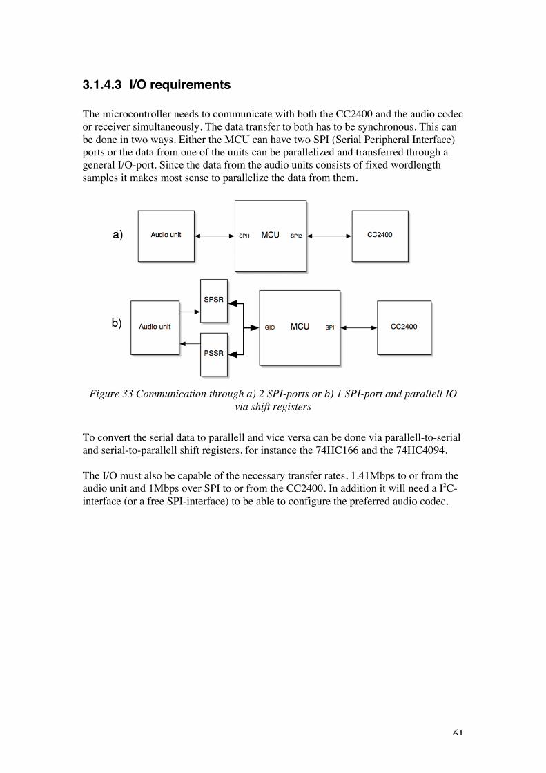
61

3.1.4.3 I/O requirements

The microcontroller needs to communicate with both the CC2400 and the audio codecor receiver simultaneously. The data transfer to both has to be synchronous. This canbe done in two ways. Either the MCU can have two SPI (Serial Peripheral Interface)ports or the data from one of the units can be parallelized and transferred through ageneral I/O-port. Since the data from the audio units consists of fixed wordlengthsamples it makes most sense to parallelize the data from them.

Figure 33 Communication through a) 2 SPI-ports or b) 1 SPI-port and parallell IOvia shift registers

To convert the serial data to parallell and vice versa can be done via parallell-to-serialand serial-to-parallell shift registers, for instance the 74HC166 and the 74HC4094.

The I/O must also be capable of the necessary transfer rates, 1.41Mbps to or from theaudio unit and 1Mbps over SPI to or from the CC2400. In addition it will need a I2C-interface (or a free SPI-interface) to be able to configure the preferred audio codec.

62

3.1.4.4 Evaluated microcontrollers

In the process of finding the right microcontroller, serveral was taken intoconsideration. When evaluating microcontrollers, the following factors have been themost important:

- Does the microcontroller meet the speed and memory requirements?- Does it have the necessary I/O-capabilities and is it easy to implement in

system?- Is it a widespread architecture with easy-to-get programming tools and

program examples?- Is it widely available at a low price?- Are development kits available at resonable prices?

Based on these criteria, numerous alternatives were evaluated. The following sectionswill give a brief description and comparison of the microcontrollers that ”made it tothe final round”. The MCUs listed in table 10 were seriously considered and closelystudied before a final decision was made.

Table 10 Comparison between seriously considered MCUs [references 30-36]Atmel Mega32L/169L

Texas Instr.MSP430F1481

MotorolaDSP56F801

Hitachi/RenesasR8C/10 Tiny

Silicon Labs.C8051F005

Architecture 8-bit RISC 16-bit RISC 16-bit DSP-hybrid

16-bit RISC 8-bit CISC

Clock speed <8 Mhz <8 Mhz 8 Mhz (80 Mhzcore)

<16 Mhz <25 Mhz

Max inst./s 8 MIPS 8 MIPS 40 MIPS 16 MIPS 25 MIPSInstr. set AVR MSP430 56800 M16C 8051Memory 2kB/1kB 2kB 2kB 1kB 2,25kBProgrammemory

32kB/16kBFLASH

48kB FLASH 16kB FLASH 16kB FLASH 32kB FLASH

I/O 1 SPI(169L:2 SPI)1 two-wire(I2C-comp)1 USART32 IO-pins

2 SPI/USART48 IO-pins

1 SPI1 SCI

1 SPI/USART16 IO-pins

1 SPI/UART1 SMbus(I2C-comp)32 IO-pins

Package pins 48/64 64 48 32 64Approx unitprice15

$6.50/$7.20 $7.00 $7.90 $1.50 $13.50

Freeprogrammingtools

Yes Yes No Trial versiononly

Yes

Developmentkit / approxretail price

STK500+501$150

MSP-STK430$100

DSP56F801EVM$350

M3A-0111Price unknown

C8051F00DK$99

15 Prices are found either from the manufacturers website or www.digikey.com. Prices are in quantitiesof 100, except Renesas R8C/Tiny for which price is given for a quantity of 1000.

63

3.1.4.4.1 Atmel AVR Mega169L and Mega32L

Early in the hardware design phase, Atmel AVR was considered the most likelyachitechture to use in the WLS. It’s a much-used processor-series with goodperformance at a resonable price. It’s also easy to program with a small and efficientinstruction set. The AVR-architecture has the disadvantage of being 8-bit, but at 1MIPS per Mhz, the performance is still good.

The only AVR-series with enough memory is the Mega-series ranging from theMega16 with 1kByte RAM and 16kByte flash to the Mega128 with 8k/128k. The”L”-units are 3.3V-compatible and thus the only ones which can be integrated into thesystem with ease. The Mega169L [reference 30] and Mega32L [reference 31] wereconsidered to be the most suitable.

While the Mega169L has the advantage of two SPI-interfaces it also has thedisadvantage of having only half the memory compared to the 32L. Even if thecommunication was made easier by being able to opt for the scheme shown in figure33a), there was always the question of memory. The 32L on the other hand has morememory and is also both cheaper and comes in a smaller package, so the extra cost ofsome external logic will probably balance out. Thus the Mega32L was considered thebest of the two.

However a more crucial problem became apparent when it came to speed. The ”L”-versions are both rated at only 8Mhz. Although the 169L has a typical performance of12Mhz at 3.3V [ref 31, figure 138], Atmel will not guarantee stable operation at thisfrequency.

If the MCU is to be run at 8Mhz, much external logic is needed to generate the 256fSclock for the audio circuits. In addition the timing between the MCU and the audiocircutry would be more complicated. The alternative would be to divide the 256 fSclock and run the controller at 128 fS or 5.64Mhz. But with an 8-bit architecture and5.6 MIPS, the speed requirements are not met. Therefore other alternatives had to betaken into consideration. The AVR Mega169L/32L suitability is summarized withadvantages and disadvantages.

+ Widespread standard with easy-to-get software and program examples+ Fast and efficient RISC architecture, 1 MIPS pr. Mhz+ 2 SPI-interfaces on the Mega169L+ Mega32L meets memory requirements, Mega169L is on the limit+ Resonable price and very good availability- Can not be run at higher frequencies than 8 Mhz- Not very powerful, 8-bit architecture and relatively low speed

64

3.1.4.4.2 Texas Instruments MSP430F1481

The MSP430-family of mixed signal devices from Texas Instruments is a series oftrue 16-bit RISC microcontrollers with a one-clock-cycle (1T) register-to-registeroperation execution time. The F148-models [reference 32] have 48kBytes programmemory and 2kBytes of RAM so they meet the RAM requirements easily. They havetwo SPI-interfaces and with no LCD-driver and no AD-converter the price of thebasic model F1481 is low. The processor is sold by many stores as well as themanufacurer themselves, but the architecture not as widespead as the AVR or 8051,so the availability of program examples is not so good. TI offers tools anddevelopment kits at low prices.

The MSP430 however has the same problem as the Mega-L-series, it is not ratedfaster than 8Mhz. Thus it has to run at 128 fS or 5.6Mhz to avoid excessive externallogic. Although this speed limitation is the same as for the AVR, the TI is stillconsidered better performance-wise since it has a 16-bit achitecture. Since all register-to-register instructions are 1T-executable, it will probably exceed five 16-bit MIPS,which is close to the performance requirement. Another drawback with the MSP430 itthat it has no I2C-compatible interface. Because of this, one SPI interface must beused for the CC2400 and one for the TLV320, and the audio transfer scheme wouldstill have to be the one from figure 33b).

In summary, the evaluation of the MSP430F1481 are as follows:

+ 16-bit RISC-architecture+ Fast and efficient instruction set+ Easily meets memory requirements+ 2 SPI-interfaces+ Very low price.- Can not be run at frequencies above 8 Mhz- Not widespread standard- No two-wire / I2C interface.

65

3.1.4.4.3 Motorola DSP56F801

The Motorola DSP56800-series is a new generation integrated MCU/DSP-hybridsdesigned for portable and integrated multimedia applications. The DSP-performanceis significantly better than with standard microcontrollers and the 16-bit unit alsoincludes peripheral like SPI and PWM-outputs. The 56F801 [reference 33] has16kB/2kB memory and runs at a blistering 40MIPS and 80Mhz core frequency. Thebuilt-in 10x clock multiplier accomodates the use of a standard 8Mhz or less crystalresonator. The package is small (48-pin) and the price not significantly higher than astandard MCU like the Atmel AVR.

The instruction set [reference 34] is somewhat more complex than for your basicMCU since it also includes some signal processing instructions. However a single-instruction 16-bit barrel-shifter, a single-instruction 16x16 multiplier and two 36-bitaccumulators included in hardware simplifies mathematical operations significantly.The major disadvantage of the DSP56800 is that it is a relatively new processorfamily and that and code examples and reference designs are not as available as formore established architectures. Also, the development tools are very expensive.

To summarize the evaluation of the Motorola DSP56F801:

+ Very powerful+ Built-in DSP-features+ 16-bit architecture+ Meets memory and I/O requirements+ Efficient C-compiler+ Small package and single power-supply+ Competitive price- Relatively new architecture, not as established as others- Development tools are very expensive.

66

3.1.4.4.4 Hitachi/Rensas R8C/10 Tiny

The Hitachi R8C/10 [reference 35] is a powerful 16-bit microcontroller built into asmall 32-pin package. Still it can be run at up to 16 Mhz and features a SPI-interfaceas well as 21 general I/O-ports. The price is very low, four times below the Atmel orMotorola-units, and the small package makes it ideal for portable solutions.

There are three alternative memory configurations of the R8C/10 with the biggest at16kB/1kB. This is the same at the minimum set in the requirements. In addition tothis, there seems to be another major problem with the R8C/10; availability. It is noteasy to find from other distributors than Rensas themselves, and the selection ofdevelopment tools seems small. Compilers and debuggers are not freely available andlitterature, code examples and other practical information is very difficult to comeacross. Also, it does not meet the IO-requirements when using the TLV320 since ithas only one SPI-interface and no I2C.

The R8C/10 seems to have great potential, but some uncertainties makes it a bit riskyto include in a reference design without prior knowledge to the processor family.

+ Good performance, up to 16Mhz+ 16-bit MCU-architecture+ Very small package+ Very cheap- Availability seems unclear, not many distributors- Not standard architecture, little literature or information available.- No development tools freely available- Does not meet IO-requirements when using the TLV320 codec.

67

3.1.4.4.5 Silicon Laboratories C8051F005

Silicon Laboratories (formerly known as Cygnal) produces high-performancemicrocontrollers based on the very established 8051 8-bit architecture. TheC8051F005 [reference 36] features a 32kB/2.25kB memory configuration and 32digital I/O-ports. Although 8-bit immediately seems like a disadvantage, the C8051-series runs at up to 25Mhz and since it executes 70% of it’s instructions in one or twoclock cycles it enables up to 25 MIPS throughput. Both in terms of speed, memoryand I/O capabilities it should be sufficient. As the only chip of the ones consideredrunning at over 20Mhz (although the DSP56F801 runs at up to 80Mhz internally) itcan be clocked with a 512fS or 22,6Mhz clock. Thus performance should not be aproblem and all necessary clocks are easily generated.

The 8051-architecture is very well established and compilers and other tools arewidely available. Silicon Laboratories also offer development kits at very reasonableprices. The only disadvantage of the C8051F005 is that it, like most others, only hasone SPI-interface and that the chip itself is more expensive than the rest. If 16 I/O-ports are sufficient, a slightly cheaper but otherwise identical model, C8051F006, isavailable in a 48-pin package.

To summarize, the evaluation of the C8051F005 comes down to the followingconclusions:

+ High performance and clock frequency+ Can be run at 512 fS+ Very well-established architecture+ Meets I/O and memory requirements+ Tools widely available at resonable cost- 8-bit architecture- Quite expensive

68

3.1.5 Conclusions:

The process of finding the right components was extensive but ultimately rewardingwork which gave insight into the hardware market as well as experience in evaluatingpossibilities and limitations of different kind of circuits.

The CC2400 was decided to be one of the components in advance, since the targetapplication is a demonstration system for just that chip. The decision to use theTLV320 audio codec was also made at an early stage since it met all the requirementsand also is highly integrated and thus quite easy to implement in circuit.

Finding the right SP-dif interface and microprocessor however, was a more difficulttask. An SP-dif receiver with an integrated sample rate converter was initially thoughtto be the solution, but no such circuits are available for 3.3V supply voltages. Thearrival of the AK4122 can change this in the near future. But for now, a receiverwithout sample rate conversion must be used. The Crystal CS8416 seems to be themost suitable one since it features a slave-mode and also 3.3V operation. However,when the AK4122 arrives this is highly likely to be preferable.

As far as microcontrollers go, there are so many models and architectures to choosefrom, and so many factors to take into account, that one just has to cut through to everget done. Consequently a few models were moved on to ”round two” and evaluatedfurher. They are the ones presented in this document.

The final decision fell on the Silicon Laboratories C8051F005, due to it’sperformance, availability, low-cost tools and well-known architecture. The greatperformance and competitive price also makes the 16-bit Motorola DSP56F801 a verystrong contender, especially if software upgradability is taken info consideration. TheMotorola is probably powerful enough to run more advanced audio algorithms, likesubband filtering or even Ogg-Vorbis fixed-rate lossy compression, in real-time. Butthe unit is less widespread, development tools are much more expensive andlitterature is scarse, so opting for a 8051-architecture was considered the safest bet.

It should also be mentioned that although the price given in table 10 seems very highcompared to the others, my instructor at Chipcon informed me that very good dealscould be made with the distributor, which would make it much more competitivelypriced. This also had significance for the final decision when it was made.

69

3.2 Audio transfer to MCU

The preferred MCU, Scilicon Laboratories C8051F005 has only one SPI-port whichwill be occupied by the CC2400 RF-module. Since the datarate to and from the audiocodec or SP-dif device is more than 1.4Mbps, creating a second SPI in software willput to much strain on the processor. A different scheme is proposed where the data isconverted from serial to parallell form and sent word-wise to the microcontroller. Themicrocontroller will read or write 8-bit words on it’s IO-port and appropriate logicwill be implemented to convert it to serial form.

3.2.1 Principle for data transfer, audio device - MCU

The audio device outputs serial data in accordance with the I2S bus specification. Foursignals are used. The LRCK clock signal indicates whether the left or the right channelis the one being transferred. SCLK is used to clock data and SDTO and SDTI are thedata input and output lines. This is shown in figure 34. Special attention should begiven to the fact that the MSB in the sample is delayed one clock cycle with respect toLRCK.

Figure 34 I2S data transfer timing diagram

The principle for the communication shceme is shown in figure 35. The data istransformed from serial to parallell form, so the MCU receives or transmits SD[15..8]in one read/write and SD[7..0] in the next.

70

Figure 35 Principle for data transfer between audio device and MCU

The control signals will tell the serial to parallell interface when to latch data onto the8-bit bus (the data-flow from the I2S-interface is continuous) when data goes from theaudio device to the MCU and when to read data from the bus when the flow is in theopposite direction. There also has to be control signals to the MCU so it knows whento write or read data on it’s IO-port and also so it knows if it is the left or rightchannel data it is dealing with.

3.2.2 Realization of data transfer, audio device - MCU

3.2.2.1 Serial-to-parallell and parallell-to-serial conversion

To make the data transfer possible, appropriate logic devices had to be found. The74HC4094N 8-stage shift-and-store bus register [reference 37] is ideal for convertingdata from serial to parallell form. It has a serial input and a strobe input. For eachclock tick the data on the serial input is shifted one step to the right in the shiftregister. When the strobe is set high, the data in the 8-stage shift register is latched tothe 8-bit storage register. Whenever the output enable signal OE is high, the contentsof the storage register is available on the parallell outputs. When OE is low, the outputis in tri-state. This is shown in figure 36.

71

Figure 36 Simplified schematics, 74HC4094N [reference 37]

To use this device to transfer data from the audio device to the MCU, a control signalis needed for the STR-input. The strobe signal has to be set high when a complete setof data is shifted to the input. This is shown in figure 37.

Figure 37 Tming diagram, transfer from audio device to MCU

As can be seen, a STR-pulse is needed every eigth BCLK cycle. Since the74HC4094N holds it output vaule constant when STR is low, the MCU can read thedata at any given time before the next STR-pulse. A delayed STR-signal, for instanceby one BCLK cycle can thus be used to interrupt the MCU to make it read it’s IO-port.The falling edge of STR provides an ideal interrupt source.

To transfer the data from the MCU to the audio codec the 74HC166N 8-bit parallell-in/serial-out shift register [reference 38] is used. It latches in an 8-bit word on theinput and shift it out serially, MSB-first. The device is activated with an active low/CE-signal and the data is latched in using the /PE-input. A logic diagram of thecircuit is shown in figure 38.

72

Figure 38 Logic diagram, 74HC166N [reference 38]

The I2S audio device reads the SDTI input on the positive edge. To assure valid datawith good timing margins on the I2S-interface, the data on the SDTI-input shouldchange state on the negative clock edge and have a stable, valid value on the positive.This can be seen from figure 34. Since the 74HC166N shifts data out on it’s positiveclock edge it should therefore be run on an inverted clock. Then the timing diagramwill be as shown in figure 39.

Figure 39 Timing diagram, transfer from MCU to audio device

The arrows indicates when the audio device reads the SDTI-data. The data is valid inthis instance and there is significant time to or from the next transition on SDTI. Thusthe timing requirements are not very stringent. The requirement for the MCU is that ithas valid data on it’s outputs before /PE is low. The falling edge of STR can thereforeprovide the interrupt source for the write too.

73

3.2.2.2 Design of logic to create necessary control signals

The control signals that needs to be generated are strobe and /PL in addition to theSCLK and LRCK signals. At first I intended to use the PWM-outputs from the MCUto generate these signals, but this proved to be unfeasible. The C8051 has aprogrammable counter array (PCA) consisting of 5 separate capture/control modulesthat can provide separate PWM-outputs. These are all controlled by a single PCAcounter/timer. The low-byte of the counter register is compared to a user definedvalue to provide a PWM output with selectable dutycycle and a frequency of 256fT,where fT is the timebase frequency of the counter (see reference 36, chapter 20 fordetails). Since the maximum fT is SYSCLK/4, the maximum PWM-frequency isSYSCLK/(4·256) or fS/2. SCLK, /PL, STR and LRCK must run at 32fS, 8 fS, 8 fS and fSrespectively, and it’s then impossible to generate them using the PWM-outputs of theC8051.

Both the strobe and /PE signals are active only every eighth SCLK cycle. Without thepossibillity of using PWM, an external counter is needed to generate them. A gate onthe output can give a high value when the counter has a specific value (e.g. ”000” or”111”) and a low value otherwise. The /PE is delayed one half clock cycle withrespect to STR and also inverted. This does not have to be done externally since the74HC166N is running on an inverted clock and therefore detects /PE one half clockcycle later. A fast ripple counter, like the 74LV4040, can also be used to create theSCLK and LRCK when it is clocked with the master clock. Since the master clock is512fS, SCLK is 32fS and LRCK runs at fS, the scheme proposed is as shown in figure40.

Figure 40 Logic circuit for generation of control signals

The 256 fS output provides a master clock signal for the audio device. The bitclockBCLK and it’s inverted /BCLK are given by the ripple counter b[5..7] = ’1’. Theoutput b8 provides a SCLK/16 signal that will be used to tell the MCU if it’s theMSW (most significant word) or the LSW (least significant word) of a sample that isbeing transferred. If LRCK and SCLK/16 are both ’1’, it’s a right channel LSW, if

74

[LRCK, SCLK/16] is [’1’,’0’] it’s a right channel MSW, [’0’,’1’] is a left channelLSW and [’0’,’0’] is a left channel MSW.

The control signals are shown in figure 41. The very high frequency MCLK and 256 fSare omitted for clarity.

Figure 41 Timing diagram for control signals

As we can see, STR is high and /PE is low at the critical points, when their respectivecircuits are supposed to latch and load data.

The component cost for realizing the control signals is:1pc. 74LV4040 ripple counter1pc. 74HC27 2x3 input NOR (also used to realize the two inverters)1pc. 74HC4094N 8-stage shift-and-store bus register1pc. 74HC166N parallell-in/serial-out shift register

These are all low-cost circuits, so compared to a MCU with two SPI-interfaces (whichwould also need some logic to be made I2S-compatible) the extra cost in hardware isnot significant. Another alternative is to integrate all of this into a small and cheapCPLD, for instance the Xilinx XE9536. The cost would then be the CPLD plus theconnector needed to program it.

In the prototype, the communication is realized with logic devices.

75

3.3 Circuit design

After deciding which components to use and developing the communications system,the next step was to design the complete circuit. The system consists of a total of eightIC’s; the C8051F005, the TLV320, the CS8416, the CC2400, the 74LV4040, the74HC27, the 74HC4094N and the 74HC166. The block diagram is showed in figure42.

Figure 42 Block diagram, wireless loudspeaker system

This diagram is highly simplified, although all major signals and buses are included.The thickest lines are buses and the thinnest clock lines, the normal ones are signallines. As can be seen, there is a fair amount of routing to be done, especially betweenthe MCU and the audio units and logic. The switch indicates the analog/digital inputselectors. Rather than opting for a electronic selector, like a mux, jumpers are usedsince they were necessary to include some other functionality anyway.

76

3.3.1 Configuration of the SP-dif receiver.

The configuration of the Crystal Semiconductor CS8416 SP-dif receiver was done inaccordance with it’s datasheet. The unit has 8 SP-dif inputs routed through a 8:2 inputMUX, but only one input was used in our application. To keep the physicaldimensions small and to avoid extra cost, the possibility to use more inputs was notutilized. To simplify implementation, the stand-alone modus is used, so the MCUdoes not need to use resources communicating with the receiver. The input-select pinsare hardwired to choose input 0, while the indicator outputs, with the exception of/AUDIO, are not used. The /AUDIO output indicates if there is valid data beingreceived and is connected to a general I/O-pin on the MCU so this can know when asignal is coming. The connection of the chip is as shown in figure 43. The SP-difinput is terminated with a 75Ω load resistance as specified by the SP-dif standard.

Figure 43 Configuration of SP-dif receiver

Special care should be taken when routing the PLL-filter. This is very sensitive tostray capacitances. To achieve correct filter characteristics and thus good jitterperformance, the layout should be like shown in figure 44. Ground connection for thePLL filter should also be returned directly to AGND independently of the groundplane.

77

Figure 44 Recommended filter layout [reference 27]

If this recommendation is followed, the PLL in the CS8416 should provide very goodjitter attenuation.

3.3.2 Configuration of the audio codec

Unlike the SP-dif receiver, the Texas Instruments TLV320AIC23B audio codec has tobe set up using a microcontroller. This is done using a 2-wire I2C-compatibleinterface. The configuration inputs can also be set up to be SPI-compatible, but sincethe MCU SPI-interface is occupied by the CC2400, I2C is used for the codec. This isset up by hardwiring the MODE and /CS inputs. The data outputs are routed to thelogic devices handling the audio transfer.

The line inputs and the mic-input is set up and filtered as recommended in thedatasheet and the electret biasing output is connected to the mic-input so the systemcan be used with all kinds of microphones. It is connected through a big resistor (10k)to prevent the DC-voltage inflicting damage on dynamic microphones.

The headphone output however, was changed slightly from the recommended layout.In their reference design, Texas Instruments used 220µF decoupling capacitors.However, simulations showed that this would compromise bass performance whenused with a low-impedance 32Ω or 16Ω headphone. Since the system is supposed tohave high-fidelity performance, a frequency response convering the entire audiblerange from 20hz-20khz (-3dB) is desirable. The capacitor size had to be increased.Figure 45 shows SPICE-simulations with two widely available alternatives, intostandard 32Ω and 16Ω headphone loads.

78

Figure 45 220µF, 330µF, 470µF decoupling caps frequency response, 32/16Ω load

The 220µF capacitor gives a 4dB drop at 20hz, which is outside of specification evenwith a 32Ω headphone. 330µF gives almost 2dB while 470µF leads to just 1dB drop,well within the demands. With a 16Ω load only the 470µF cap fulfilled the spec.However, from our supplier 470µF capacitors turned out to be much larger physicallythan 330µF. Because of this, and also since 16Ω headphones are quite rare, the middlevalue was chosen as a compromise. The complete connection of the TLV320AIC23Bis as shown in figure 46.

Figure 46 Configuration of audio codec

79

3.3.3 Configuration of the RF-transceiver

The Chipcon CC2400 RF-transceiver is in this application set up identically to the2400DB demonstration board. The microcontroller interface is connected forhardware packet handling support. This allows for hardware insertion of preambles,sync-words and CRC in the data stream by the CC2400. If this does not need to beutilized, the relevant pins can just be ignored by the MCU. It uses it’s own 16Mhzcrystal and two voltage levels (1.8V core and 3.3V IO). Data transfer andcommunication is, in addition to the pins used for packet handling, done through astandard SPI-interface, connected to the MCUs SPI-pins.

The CC2400, being an RF-device, is rather sensitive to PCB-layout. Separate voltageand ground planes, as well as low impedance connections from all critical nodes tothese, is highly recommended. The layout itself was done by Chipcon, usingprofessional CAD-tools, and will not be reviewed in detail in this thesis. Interestedreaders are reffered to the Chipcon CC2400 datasheet and the complete PCB-layoutincluded in appendix 5.

The connection of the Chipcon CC2400 RF-transceiver is shown in figure 47.

Figure 47 Connection, Chipcon CC2400 RF-transceiver

80

3.3.4 Configuration of the MCU IO

The C8051F005 IO-system uses a Priority CrossBar Decder to assign the internaldigital resources to the IO-pins. This gives the designer full complete control overwhich functions are assigned, limited only by the physical amount of IO-pins in theselected package. A block diagram of the system is displayed in figure 48.

Figure 48 C8051F00x IO-system functional block diagram [reference 36]

The CrossBar assigns the selected internal digital resources to the IO-pins based onthe Priority Decode Table [reference 36], shown in figure 49. It starts at the top withthe SMBus, which means that when it is selected it will be assigned to P0.0 and P0.1.The decoder always fills IO-bits from LSB to MSB starting with Port 0, then Port 1,finishing if necessary with Port 2. If a resource is not used, the next function in thepriority table will fill the priority slot.

81

Figure 49 C8051F00x priority decode table [reference 16]

In the design of the wireless audio system, the SMBus will be used to configure theaudio codec, thus it must be assigned. Next, the SPI-interface will be used to senddata to and from the CC2400 RF-transceiver. The UART will not be used, neither willthe timer outputs, since all control signals are generated by external logic. Theinterrupt input /INT0 will be used however, since the MCU must receive an interruptwhen sending or receiving data. The /INT1 is used by the Chipcon CC2400. The/SYSCLK output will also be used to clock external circuits, while the rest will beunused. This results in a configuration of the CrossBar Decoder as shown in figure 50.

82

Figure 50 Configuration of MCU IO CrossBar Decoder

The IO-pins P0.0 to P0.7 will be assigned to digital functions as shown in figure 50,while the rest of the ports will be general IO (GIO) ports used to transmit and receivenecessary data and other signals. The complete circuit schematics (appendix 4) showsthe entire allocation of the IO-pins for the MCU and the complete connections for thecircuit.

83

3.3.5 The finished circuit

The complete circuit with all connections are shown in figure 51 (a bigger, higherresolution version is found in appendix 4). For clarity some connections are shown asbuses.

Figure 51 Complete circuit diagram

In addition to all the circuits including logic, the power supply and analog connectionsare also shown. Some of the lines are routed through a 10-pin connector to provideextra flexibility. One jumper can choose between normal mode and digital loopback.In the latter mode, the audio output from the codec is fed back directly to it’s inputs.This gives the user the opportunity to test if the codec works, if it’s properly set upand so on without having to connect or program the entire system. This should alsoenhance the circuit’s testability significantly, since locating errors will be mucheasier. If the digital input is selected, this is routed back to the codec in loopbackmode. The second jumper selects master or slave mode for the MCU, while the thirdone is a digital/analog input selector. The jumper settings are shown in figure 52.

84

Figure 52 Jumper settings

To further enhance testability, several zero-ohm resistors are put on critical lines. Inaddition, the circuit has two logic analyzer connections, compatible with the standardlogic analyzer port of figure 53.

Figure 53 Logic analyzer standard connection

The pinout is such that the logic analyzer can be used to both monitor all criticalsignals under operation, but also to take directly control over the audio codec and theSP-dif receiver if it is necessary during testing. This is useful if for instance the MCUfor some reason fails to provide the clock signals or control signals necessary tooperate the other devices and thus test them. The complete logic analyzer port pinoutis shown in figure 54.

85

Figure 54 Logic analyzer connections

In addition, there are two LEDs in the circuit to indicate power-on and /AUDIO fromthe SP-dif receiver respectively. Also, a third LED is connected to a MCU IO-portand can be used for whatever the user finds desirable.

86

4 Analysis of Lossy Compression Algorithms

The lossy compression algorithms examined were written in C, ensured to be wav-compatible and run on a Apple Powerbook G4 laptop-computer. The compressed anddecompressed files were analyzed in Matlab to see how big the errors were. A much-used measurement of loss in a compressed audio file is the ratio between the signalpower and the error power, also referred to as the SER. Since the error (or noise-level)in a lossy compressor should follow the signal level (to stay below the maskingthreshold), SER gives a better indication of it’s loss than you get by just looking at theerror itself. Also, a plot should be made to ensure the error level actually follows thesignal-level. A Matlab-script was written that calculates the SER and the maximumabsolute error and plots the signal and the error as a function of time. The source-codeas well as the Matlab-script is given in appendixes 6 and 7. The maximum absoluteerror is simply the factor between the maximum error and the maximum allowablesignal level while SER is given by the equation:

Eq. 34 SER = 10 ! log

1N

(x[n])2i=0

N

"1N

(e[n])2j=0

N

"

#

$

%%%%

&

'

((((

= 10 ! log(x[n])2

i=0

N

"

(e[n])2j=0

N

"

&

'

((((

#

$

%%%%

The analysis was done with a file called ”littlewing.wav” a recording of myselfplaying guitar. The recording has much dynamics, so performance could be evaluatedat both low and high signal levels, a fairly wide spectrum but even more importantly,a very clear and unedited sound. When doing subjective listening-based quality tests itis important to have a reference that sounds both natural and familiar. Then distortionand colouring of the sound can more easily be identified since one knows how it’ssupposed to be like. The necessity of subjective listening tests is obvious. Althoughthe SER together with an error plot gives a good indication of how much loss there is,it tells quite little about the nature of the loss. Lossy compression algorithms useperception-based models, whose quality can affect the resulting fidelity significantly,even if the loss is the same in absolute quantity.

Figure 55 shows the waveform and spectrum of the used test file.

87

Figure 55 Waveform and spectrum, "littlewing.wav"

4.1 Reference for comparison; 8-bit and 4-bit LPCM

To put the numbers into perspective, the tests are first presented on 8-bit and 4-bitLPCM requantization of the audio data. When doing LPCM quantization, the 6dB perrule tells us the maximum acheivable SNR, the resolution, is 6"B, where B is thenumber of bits. Since LPCM quantization does a random roundoff, the noise is almostwhite and the level is thus constant and about 6"B dB below the maximum signallevel. For a maximum level signal, the SER would then be identical to the resolution,but for normal music signals it will be significantly lower as the results for”littlewing.wav” show.

Figure 56 Performance measurements, 4-bit and 8-bit LPCM

88

Table 11 Performance, 8-bit and 4-bit LPCM8-bit LPCM 4-bit LPCM

SER 28.8dB 8.3dBMaximum error 0.004 0.07

As we can see, the SER is well below the resolution. This is of course because thesignal level and thus signal power is lower than maximum while there is no relatedshaping of the noise. We can clearly see that the quantization noise is white, at leastfor the 8-bit version. For 4-bit there actually is some visible correlation between thesignal and the noise. It can be shown that LPCM quantization noise in reality is notcompletely white, but does produce some distortion, especially for low-level signalsor very coarse quantizations. Since distortion sound worse than white noise this isoften compensated for by adding random noise, also called dithering16.

It should also be noted that the noise is not in any way psychacosutically shaped.When the signal level is low, the masking threshold is also low, but the noise is stillhigh. It is then very audible. Perceptive-based shaping of the noise can providesignificant improvements in audio fidelity, even when the SER value is the same.Both 8-bit and 4-bit LPCM is classified as low-fidelity.

4.2 Analysis of 4-bit DPCM

A 4-bit (or 4:1) DPCM compression algorithm was written and compiled on thePowerbook. It uses the scheme described in the DPCM theory chapter with anexponential quantization table. The quantization is showed in table 12.

Table 12 DPCM quantization tableCode 0 1 2 3 4 5 6 7Difference 0 -16536 -4096 -1024 -256 -64 -16 -4Code 8 9 10 11 12 13 14 15Difference 0 4 16 64 256 1024 4096 16384

The source-code is given in appendix 6. As one can see, the quantization spaces aresmall for low levels and very large for high levels. It’s therefore assumed that theDPCM will perform poorly when the levels (or rather, the differences, since firstorder prediction is used) are high. Since some music recordings are very dynamic, it’slikely that DPCM will be less suitable in a hifi-application than for voice-coding,where the levels are usually quite low. The algorithm was tested for performanceusing ”Littlewing.wav”.

As expected, the 4:1 DPCM compressor was very fast, but did not perform well whenit came to audio quality. Especially for loud signals, the quantization error is huge (ascan be seen by looking at it’s exponential quantization table) and the distortion isclearly audible. At low volumes, the noise-level is far better than for 4-bit LPCM

16 See appendix 2, ”Data converter fundamentals” for details

89

quantization, and the music quality is improved somewhat. But the error ”bursts” asseen in figure 57 are far above the masking threshold and are clearly audible.

Figure 57 4:1 DPCM performance measurement, "Littlewing.wav"

As table 13 shows, a calculation of SER despite prediction gave little improvementover 4-bit LPCM17, but still the shaping of the noise gave a clear improvement insubjective performance outlining the need for listening tests as well as measurements.Still, the performance is nowhere near acceptable quality. 4-bit DPCM is suitable forvoice applications, but more or less useless on high-fidelity audio.

Table 13 Performance 4-bit DPCM, ”littlewing.wav” (see text)SER 8.5dBMaximum absolute error 0.70Complexity estimation Approx. 100 inst./sample 17 It can be shown that if the variance in the difference between samples (i.e. the predicted residual),*2

∆x, is larger than the variance of the samples, *2x, prediction will give more distortion since the bit-

rate/distortion ratio is dependent on variance. Also, the nonlinear quantization can yield worse resultswhen the signal is in the area where the quantization steps are larger than the linear ones (i.e. >4096).For most music signals however, one would be likely to get an improvement with DPCM over LPCMand for speech signals even more so.

90

4.3 Analysis of IMA ADPCM

The algorithm written to test ADPCM was made compliant with the IMA ADPCMstandard. The reader is referred to the IMA ADPCM theory chapter and the source-code for a more detailed insight in how it is made. It was tested with the same file asthe DPCM algorithm for a subjective (listening test) and an objective (Matlab)evaluation of audio quality. The result was a massive improvement over normalDPCM. There still is some audible distortion on loud or dynamic passages, butnothing compared to DPCM. Subjectively, IMA ADPCM does provide fairly high-fidelity music, the quality is resonable for background music or casual use, but stillnot sufficient for critical listening over a high-performance hifi-system. Again, thenoise ”bursts” are clearly above the masking threshold, although nowhere nearDPCM, while the average background noise is very low, almost inaudible.

The analysis done with Matlab is given in the figure and table below.

Figure 58 IMA ADPCM performance measurement, ”Littlewing.wav”.

91

The errors are now much smaller, between –0.05 and 0.05 in amplitude and with avery low nominal noise level. We can also see that it clearly follows the signal leveland thus also the hearing threshold. The calculated values are given in table 14.

Table 14 Performance 4-bit ADPCM, ”littlewing.wavSER 32.5dBMaximum absolute error 1.23Complexity estimation Approx 250 inst./sample

As we can see, the SER har increased dramatically. 32.5dB is still not true hi-fiperformance, even when the noise is phychoacoustically shaped, but compared to the8.5dB achieved with the DPCM algorithm the improvement is very significant indeed.As we can see, it is still ”bursts” of distortion at dynamic passages which dominates.With less dynamic music the subjective results as expected were better. The hugemaximum absolute error in table 14 is not as worrying as it seems, it’s just a result ofthe very first prediction being way off, since the index-variable and the previoussample variable must be given start values before the first run (see source-code).

The penalty of using ADPCM is increased complexity, it is about 2.5 times slowerthan the basic DPCM algorithm. With effective programming however, real-timeIMA ADPCM should be possible to implement on a resonably powerful MCU.

4.4 Analysis of µ-law

Both algorihms above produce a 4:1 compression ratio while, in the applicationintended, 2:1 compression is sufficient. However, doing for instance 8-bit DPCM withthe method described above would require a 8-level search-tree (ending in 255nodes), which would make it very ineffective (approximately a 100% increase incomputaton time). It would be as slow as, and probably not better than, IMAADPCM. An 8-bit translation of the ADPCM algorithm would also be difficult orimpossible to implement on a MCU. The stepsize-table would be very large andprobably not fit in the limited memory available in such a system.

The µ-law algorithm is an algorithm made for 2:1 (16-bit to 8-bit) compression andfrequently used in digital telephony (it’s also used in DAT-recorders with longplay-function). It is adaptive since the quantization depends on the input level and providesa significant improvement in dynamic range over 8-bit LPCM. The reader is referredto the theory section for details. The algorithm is standardized, fast and easy toimplement. A µ-law codec was developed in C and run on the Powerbook using thesame test setup as for DPCM and ADPCM.

92

Figure 59 µ-law performance measurement, ”Littlewing.wav”.

The 8-bit µ-law algorithm is clearly better than the 4-bit ADPCM, which was asexpected. In numbers, the performance is as shown in table 15.

Table 15 Performance 8-bit µ-law, ”littlewing.wav” and ”speedtest.wav”SER 42.6dBMaximum absolute error 0.022Complexity estimation Approx. 200 inst./sample

During programming and testing, it became evident that µ-law is actually faster thanADPCM and provides higher audio quality, though at twice the output bitrate. Sincethe bitrate still is within the requirements, µ-law is definetely a viable alternative thatprovides decent fidelity music quality and is fast and well-tested.

Another advantage with µ-law that became evident when listening is that the errorsare better spread throughout the signal range. The noise is, as it should be, highest forloud signal levels, but the ”bursts” found in DPCM and ADPCM are not nearly aspresent in µ-law. The error follows the signal level, and thus the masking threshold, in

93

much better way. Subjective listening tests confirm and reinforce the superiority µ-law has over 8-bit LPCM and also IMA ADPCM. If the wireless loudspeaker systemis to use lossy compression with a standard algorithm, µ-law is regarded the mostsuitable of the ones tested.

4.5 Reference for comparison II: MP3

Although MP3 is impossible to run on a small MCU-system and therefore isirrelevant when it comes to implementation, it serves well as a performance reference.MP3 is well-known, there is a general subjective opinion of it’s quality, an analysis ofMP3 will help to put the numbers achieved by the above compression methods intoperspective.

The ”littlewing.wav” audio-file was compressed and decompressed using what isconsidered the best MP3-codec, LAME. The performance was measured using thesame error-calculating Matlab-script as for the other algoritms. Speed measurementswere not taken, since the MP3-application utilizes special hardware within thePowerbook (like the G4 Velocity Engine and more) and a comparison therefore wouldnot be representative18.

Measurements were made on 128kbps, 192kbps and 256kbps MP3. 128kbps isgenerally considered to be of good hifi-quality. It is often reffered to as ”CD-quality”or ”near CD-quality” in the litterature, but blind-tests have shown that MP3 is notquite transparent at this bitrate. 192kbps is considered to be of very high quality, inmost cases transparent, but with slight audible loss on some material when playedback over high-end stereo systems and under near-optimal listening conditions.256kbps is gererally accepted to be completely transparent, as blind tests have notconsistently proved audible differences. However, the most discriminate audiophilesalso claim this this bitrate is inferior to CD, pushing the envelope for even moresophisticated algorithms like AAC. The measurements are summarized in table 16,128kbps and 256kbps is shown in figures 60 and 61.

Table 16 Measured performance, LAME MP3, ”littlewing.wav”Bitrate SER Max error128kbps 49.0dB 0.011192kbps 60.4dB 0.0027256kbps 67.1dB 0.0011

18 Velocity Engine is a special instruction set within the G4, used to increase multimedia performance.It also has a dedicated maths co-processor and other special hardware which is not utilized by thecompression routines written for this thesis. The encoding of a 10min wav-file takes less than 20s witheither MP3 or AAC on the 1Ghz Powerbook, almost as fast as the simple DPCM codec. To writededicated compression programs that utilizes the Mac hardware is beyond the scope of, and not thefocus of, this thesis.

94

Figure 60 Measured performance, 128kbps MP3, ”littlewing.wav”

95

Figure 61 Measured performance, 256kbps MP3, ”littlewing.wav”.

We can see that MP3 is better than any of the above methods, even at 128kbps bitrate(12:1 compression ratio). This proves that much can be gained using advancedalgorithms. Unfortunately, dedicated hardware or powerful processors are needed forreal-time implementation. If low compression ratios (2:1 to 4:1) are sufficcient, evensimple algorithms can give quite good results. However, for ratios below 2:1,dynamic quantization does not seem to be a good alternative due to the ”bursts” ofdistortion and the fast-rising complexity of the quantizer due to the number of outputlevels rising exponentially with the number of bits.

96

4.6 iLaw: a low-complexity, low-loss algorithm.

For this part of the project, a low-loss compression algorithm was designed especiallyto meet the requirements of the wireless loudspeaker system, and to be an alternativeto lossless compression if implementing the latter proved unfeasible. The demands areas basic as they are fundamental:

- < 1Mbps bitrate (some headroom should be available for otherinformation).

- Very low computational complexity- High-fidelity audio quality.

Since the DPCM quantizer and ADPCM tables quickly increase in size andcomplexity with the number of bits in the compressed stream, they were discardedfrom further development. Rather, the coding is based on µ-law coding, whosecomplexity is in principal independent of the number of output bits. The minimumcompression is given by:

Eq. 35 WLO =bps2 ! fS

=1 !106

2 ! 44,100= 11.3

Where WLO is the maximum output word length. Since some headroom is desired, a10-bit version of the µ-law encoding scheme was developed. This would allow for a15-bit dynamic range using a 3-bit exponent and a 6-bit mantissa as described in theµ-law theory section. Thus, the 10-bit output word will be on the form:

Figure 62 10-bit µ-law data format

Since the exponent can hold a zero count up to 8, the sign bit holds the MSB and themantissa 6 LSBs, the dynamic range is 15-bits. It’s just an expansion of the standard8-bit µ-law coding, which has a 4-bit mantissa and thus 2-bits lower performance.

In addition, to minimize the number of high values (with correspondingly highquantization errors), second order prediction is performed. This can be done at verylitte computational cost, since e2[n] = e1[n]-e1[n-1], where e1[n] = x[n]-x[n-1], asshown in the theory section where prediction is discussed. To avoid accumulation oferrors, the output value fed back has to be decoded from the compressed data. Thecomplete predictor and encoder was made like shown in figure 63.

97

Figure 63 Flowchart, iLaw encoder designed for this thesis.

In the case of second order prediction, the filter is on the form H(z) = 2z-1-z-2,however, no multiplications are used since the residuals are calculated as shownearlier. The differences are also rounded to 16 bits while they may actually be 17.Since the 10-bit µ-law throws away the LSB anyway (it has 15-bit dynamic range; thesignbit, 8 zeros and the 6-bits mantissa is what it at most can hold) this will not lead toany further degradation of the signal quality and the encoder’s complexity is reduced.

The decompression is very simple and easy to implement, it will be the same filterand the same decoder as used in the compression.

Figure 64 Flowchart, iLaw decoder designed for this project.

This special iLaw codec was written in C and compiled for Mac OS-X to enable aperformance evaluation. The results for the same tests as the others are shown in table17.

98

Table 17 Performance iLaw codec, ”littlewing.wav”SER 49.5dBMaximum absolute error 0.0055Complexity estimation Approx. 250 inst./sample

As can be seen, the results are significantly better than for the traditional µ-law codec.Actually, they exceed the measured numbers achieved with 128kbps MP3, andsubjective listening tests also show very little degradation of signal quality.

Figure 65 Measured performance, custom codec, "littlewing.wav".

This codec provides high-fidelity performance and should also be quite easy toimplement in an MCU. It is thus a viable alternative to lossless coding.

99

4.7 Notes about the performance measurements

Although measurements for only one reference file are shown in this report, thecodecs were tested on several music tracks to ensure that the results wererepresentative for the algoritms and not caused by special circumstanses. The”littlewing.wav” file has both a quite large dynamic range and a wide spectrum, so itwon’t mask any bad performance. The check done with other files confirmed this.

The signal-to-error ratio is a standard method to evaluate compression performance.However, even though it gives an accurate representation of the error magnitude, itdoes not take into consideration the more advanced properties of the hearing.Although the error levels can be quite high, one must remember that they consistentlyfollow the masking threshold and because of this may still not be very audible. Howaudible depends on the quality of the encoder. No good measurement methods havebeen developed that include distortion or error perceptability, consequently evaluationwas also done through subjective listening tests. Actually, they corresponded quitegood with the measurements, 128kbps MP3 and the iLaw codec were evaluated to beof about the same quality and offered very good performance. On standard 8-bit µ-law the distortion was clearly audible, while it with the 4-bit codecs was directlyannoying.

Estimations of complexity were done by compiling a single compression run with theSDCC MCU-compiler and count the instructions in the resulting assembly-file. Itshould be noted that this was a very rough estimation since no data retreival orsending operations were included, the variables were just given certain values. Also,the code was not significantly optimized for the MCU. But although these estimationsare not very precise, they give an indication on how demanding the differentalgorithms are. To do a full implementation of every codec would be too much workand at this stage rather pointless, since the estimations were just meant to indicatewhether or not the different encoders are at all feasible to implement in an MCU. Andsince there are 512 instructions available per sample, they are.

100

5 Design of Lossless Compression AlgorithmThe goal for the WLS is to use lossless compression to restrict the datarate to withinthe 1Mbps capability of the RF-transceiver while maintaing full audio quality. Inaddition, since the algorithm must be able to run on real-time using only a 8-bit MCU,it has to be very fast. Different solutions were tested by the means of writingprograms in C doing the necessary functions and then evaluate them by compiling forOS-X and run them on wave-files.

As explained earlier, lossless compression algorithms necessarily produce variablelength output words. This since it continuously adapts to the ”compressability” of theinput signal (in other words, continuously eliminating redundancy). For shorterperiods one can actually experience a negative compression ratio, which complicatesreal-time use. Buffering must be implemented, and if the buffer runs empty, one hasto enter some kind of lossy-mode until it fills up again. This will only happen for veryshort time-periods and will probably not be audible. However, it is advantageous ifthe lossless algorithm does not produce excessive word length even in a worst-casescenario.

Due to the signal-dependent performance of lossless compression, a range of wav-files were used to characterize the algorithms with a resonable accuracy. 6 files werepicked to be the basis of the evaluations done in this part of the thesis. These musicpieces are of a very varied nature and should combined give a good estimate of real-life perfomance. The files are listed in table 18, and their waveforms and spectrashown in figures 66 and 67. When results are given, references are made to the wav-file(s) for which they were found.

Table 18 Wav-files used for characterization of lossless algorithmsFilename Contents Characteristics”Littlewing.wav” Recording of myself playing the

intro to Jimi Hendrix’ ”LittleWing” on guitar, 38 seconds.

Quite dynamic, some reverb,solo instrument only.

”Percussion.wav” Ed Thigpen - ”Could Break”,60sec excerpt.

Just percussion, much highfrequency content due to cymbaland hi-hat use.

”Rock.wav” Stevie Ray Vaughan –”Couldn’t Stand The Weather”,50sec excerpt.

Rock/blues quartet. Fast, loudand energetic.

”Classical.wav” Berlin PhilharmonicalOrchestera – ”Eine KleineNachtmusik” – allegro. W.A.Mozart, 60sec exc.

Symphony orchestera. Quiet inplaces.

”Jazz.wav” John Coltrane – ”Blues to You”,60sec excerpt.

Instrumental, medium dynamicsand loudness.

”Pop.wav” Robbie Williams ft. KylieMinouge– ”Kids”, 60secexcerpt.

Typical modern pop recording,very loud all the time, highlycompressed

101

Figure 66 Waveform of, from top to bottom, "littlewing.wav", "percussion.wav","rock.wav", "classical.wav", "jazz.wav" and "pop.wav", Audacity

The waveform and FFT give a good indication of compressability. The louder thewaveform, the higher the entropy. The effectiveness of prediction (how much theentropy is reduced) is as explained in the theory chapter dependent on the high-frequency content. Since the entropy is related to the signal power and the entropyreduction possibility to the HF-content, the ”compressability” could to some degreebe quantified using the mean signal power level and the spectral centroid (the spectral”center of gravity”) as well as by looking at waveforms and FFTs. The Matlab-files inappendix 7 includes calculation of both signal power (the SER calculator) and spectralcentroid for the interested reader to explore.

For simplicity all files are, as can be seen, mixed down to mono. The gain of usingchannel decorrelation was tested seperatly. To reduce the workload when testing otherparameters like prediction and coding schemes, only mono codecs were used duringthis phase of the developement.

102

Figure 67 Spectrum of the "littlewing.wav", "percussion.wav", "rock.wav","classical.wav", "jazz.wav" and "pop.wav”, Audacity

As we can see the files characteristics are very different, some have much high-frequency content and others less, while some are definetely much louder than theothers. Combined, these files should give a good indication of how well the testedalgorithms will perform.

It should be noted that when the ”pop.wav” file in table 18 is decribed as ”highlycompressed” it is not with reference to any data compression, but to amplitudecompression. What is done is that the volume of all the tracks in the recording istruncuated and amplified to full level using an amplitude compressor. This techniqueis very commonly used in pop recordings to maximise perceptability over low-fidelityplayback systems like radios, car-stereos and TVs. Popular music is sold throughmass media and it is important that the music is ”catchy”, i.e. easy to remember evenwhen listening to it casually or with low-quality sound. When everything is loud, it’seasy to perceive. Audiophiles will of course argue that this makes the music ”flat” andlifeless, but they are not the target audience anyway. However, this poses a problemwhen it comes to data compression as well. Since the signal amplitude is very high atall times, the entropy is also high and the music is difficult to compress. Losslesscompression can because of this be expected to have a lower performance level onsuch recordings and they are therefore often used as worst-case scenario benchmarks.

103

5.1 Coding method

One of the most crucial steps in a lossless compression algorithm is the entropycoding. It should be fast, memory efficient and at the same time eliminate almost allredundancy.

Huffman-coding and adaptive huffman-coding were discarded during theoreticalevaluation due to the difficulty of necessary estimations for the former, and thecomputational complexity of the latter. Also, studies showed that very few excistingprograms use Huffman-coding, the approach used in almost all available software isRice-coding.

Rice-coding has the advantage of being very fast, easy to implement and there is noneed to store tables. The clear disadvantage of Rice-coding, as shown in the theorychapter, is the huge codelengths produced when there is significant overflow (that is,when the real sample value is significantly larger than the k-bit estimated value that issent uncoded). Thus the estimation of the factor k is very critical. A fast method tocalculate k has been shown, but this calculation is still the most demanding bitcomputationally. One can trade off effectiveness for speed by using the same k for alarger number of samples, but then some very long codes will be produced. Asmentioned, this is much more critical in a real-time system than in a computerapplication.

Another alternative is the Pod-code. Here, the overflow is also sent uncoded. Aheadof it comes a number of zeros that indicate how many bits the overflow is.Consequently, the codelength has been reduced from (overflow+1+k) for Rice-codingto (2"log2(overflow)+k) while the prefix-property has been preserved.

5.1.1 Evaluation of Pod-coding and Rice-coding

A Rice-codec and a Pod-codec was written in C and run on wavefiles to examineeffectiveness. Both are included in appendix 6. The most interesting thing was to seehow the algorithms behaved for different calculations of k. So the reader does nothave to look it up, the calculation of k is repeated:

Eq. 36

k =min k' 2k'N ! A

Where A is the accumulated sum of previous residual magnitudes and N is a count ofresiduals. Programmed in C, this translates to:

for( k=0; (N<<k)<A; k++);

The two critical factors in this calculation is how often it is done and also how often Aand N should be reset. Ideally one should calculate a new k for every sample.However, this will slow down the codec, since this calculation is the most complex in

104

the algorithm. If k is calculated too rarely, the effectiveness will be reduced, thequestion is by how much. Also, one has to reset N and A with some interval, so theydon’t use up too much memory. However, to do it too often will decrease theperformance since less previous samples are averaged.

If A is to be limited to 3 bytes, it has to be reset at least every 256th sample, then N iskept within 1 byte. If A is limited to 4 bytes, it has to be reset at least every 65536thsample and N will use 2 bytes. Remember than in an 8-bit microcontroller, the timeused to increment A and N will increase significantly if their length is large, a 32-bitaddition is much more time-consuming than a 16-bit, and the incrementation must beperformed for each sample passed. As a consequense an upper limit to the reset cyclewas set at every 256th sample19.

It should be noted that using the same k for several samples will give mostperformance decrease for signals with much high frequency content. This is obviousbecause the sample values then will vary more within such a frame, and a largernumber of samples are likely to produce much overflow. Prediction is earlier shownto be equivalent to a high-pass filtering of the signal, and the effect of a non-ideal kshould be different when prediction is performed. To see if this has a big effect on theperformance of the two coding methods, they were tested both without prediction aswell as with first-order prediction.

The results with are shown in following tables, without prediction and with with firstorder prediction.

Table 19 Performance of Rice- and Pod-coding, A and N reset every 256th sample,no prediction, ”littlewing.wav”

Calculationfrequency, k

Rice - filesizereduction

Rice - maxwordlength

Pod - filesizereduction

Pod – maxwordlength

Every sample 25.8% 29 bits 25.3% 20 bitsEvery 4th 25.4% 48 bits 25.2% 22 bitsEvery 8th 25.3% 48 bits 25.1% 22 bitsEvery 16th 25.3% 48 bits 25.0% 22 bitsEvery 32nd 25.1% 52 bits 24.9% 22 bitsEvery 64th 25.0% 64 bits 24.8% 22 bitsFixed k = 6 -28.0% 371 bits 14.4% 26 bits

19 Experiment were done with A incrementing over a larger number of samples between each reset, butthe gain in compression ratio was not significant and therefore considered not to be worthwileexploring further due to the given limitations in processing power.

105

Table 20 Performance of Rice- and Pod-coding, A and N reset every 256th sample,1st order prediction, ”littlewing.wav”

Calculationfrequency, k

Rice - filesizereduction

Rice - maxwordlength

Pod - filesizereduction

Pod – maxwordlength

Every sample 42.0% 30 bits 41.8% 20 bitsEvery 4th 42.0% 44 bits 41.7% 20 bitsEvery 8th 41.9% 52 bits 41.7% 20 bitsEvery 16th 41.9% 62 bits 41.6% 20 bitsEvery 32nd 41.8% 85 bits 41.6% 20 bitsEvery 64th 41.8% 116 bits 41.6% 21 bitsFixed k = 6 31.8% 172 bits 37.5% 24 bits

As we can see, the Rice codec performs significantly better when k is calculated forevery singe sample. This is not unexpected as table 4 in the theory chapter shows thatRice is the more effective code for very low overflow values. It was a bit surprising tosee that the Rice encoder help up even when a new k was calculated only every 32ndor 64th sample. However, the difference evens out, and with a fixed k Rice codingperforms very badly. It was also a bit surprising to see that with first order predictiontoo, the Rice codec held up very well even with the same k over frames of 64 samples.This, along with the big gain when doing the prediction, indicates that there is quitelittle high-frequency content in the signal. To validate this assumption, as well as theone stating a decrease in performance for the combination big frames and much HF-energy, tests were done on ”percussion.wav”; a recording of percussion instrumentswith much high-frequency energy. The simulations were done for the two extremes, anew k for each sample, and a new k for every 64th sample.

Table 21 Performance of Pod- and Rice-coding with HF-rich file, no prediction,"percussion.wav".

Coding Cal.frequency of k Filesize reduction Max wordlengthRice Every sample 31.7% 2397 bitsRice Every 64th sample 31.4% 2397 bitsPod Every sample 31.5% 26 bitsPod Every 64th sample 31.4% 26 bits

Table 22 Performance of Pod and Rice coding with HF-rich file, 1st orderprediction, "percussion.wav".

Coding Cal.frequency of k Filesize reduction Max wordlengthRice Every sample 36.3% 1105 bitsRice Every 64th sample 36.0% 2917 bitsPod Every sample 36.2% 23 bitsPod Every 64th sample 36.1% 26 bits

Again the Rice-codec performs surprisingly well even when the same k is held over64 samples. But the gap to the Pod-codec has closed, which shows that k is not asaccurately estimated when there is much high frequency energy. One should also notethat the process of prediction has much less effect on the percussion track. This is

106

obvious since high frequencies means big differences between adjacent samples. Thatthe compression ratio is as good as it is, is probably due to the fact that parts of thistrack are quite silent and in these periods the datarate produced by the encoders isquite low.

There is no doubt however, that the worst-case performance of the Pod-encoder ismuch better than for the Rice-encoder. As the results show, the maximum wordlengthfor the Rice-coding increases dramatically even when the parameter calculationfrequency is reduced to every fourth sample. In a computer compression program thisis not a problem, in a real time system, the huge variance in wordlengths can representa very big problem. When there is much high-frequency content, the wordlengths canreach thousands of bits. It should be noted that the identical results in the first test ofthe percussion track is probably due to the biggest miss being at the very first sample,where k is set to the initial value 6. The track starts with a very loud cymbal smashbeginning at it’s very first sample.

The average performance of the Rice and Pod encoder in all the tests listed above isshown in figure 68. The cases with a fixed k are excluded from this average, since thatis something than would not be considered in any final algorithm and thus has littlerelevance when it comes to evaluating the practical results.

Figure 68 Encoding performance and worst-case word length, all tests averaged

The conclusion after examining and comparing Pod-coding and Rice-coding is thatthe gain of using Pod-coding is most significant in real-time systems, where theexcessive wordlengths produced in some cases by Rice-coding can cause seriousproblems and would demand a big buffer not to interfere with the data throughput. Incomputer compression applications, where real-time operation is not needed, the Pod-coding is unlikely to give any performance improvement. As figure 68 shows, theperformance is in the Rice-codings favour, although only by 0.2%. Rice-coding isalso the preferred method in almost all commercial lossless audio codecs. Butcomputer programs is not the target application for this thesis. The codec is to be used

107

in a low-power, low-memory real-time systems, and due to the enormous differencein worst-case behaviour Pod-coding is clearly considered the better alternative of thetwo.

5.2 iPod: an attempt at improving the Pod-coding

When developing a lossless encoding scheme, or anything else for that matter, youalways try to find ways to improve on the algorithms existing today. One way ofimproving the Pod entropy coding that hasn’t been shown before is here suggestedtogether with test results. The coding is called iPod for improved-Pod20. The idea is toput the sign-bit into the coded prefix/overflow but still preserve the crucial prefix-property. The scheme, together with the gain in output sample wordlength is shown intable 23.

Table 23 Regular Pod-coding vs. iPod-codingOverflow Pod-code iPod-code

(res > 0)iPod code(res < 0)

Changein codenumberof bits

Gain inbits duetoremovalof signbit

Netgainin bits

0 1 01 10 -1 1 01 01 0010 1101 -2 1 -12 0010 0011 1100 0 1 13 0011 000100 111011 -2 1 -14 000100 000101 111010 0 1 15 000101 000110 111001 0 1 16 000110 000111 111000 0 1 17 000111 00001000 11110111 -2 1 -18 00001000 00001001 11110110 0 1 19 00001001 00001010 11110101 0 1 110 00001010 00001011 11110100 0 1 111 00001011 00001100 11110011 0 1 112 00001100 00001101 11110010 0 1 113 00001101 00001110 11110001 0 1 114 00001110 00001111 11110000 0 1 115 00001111 0000010000 1111101111 -2 1 -116 0000010000 0000010001 1111101110 0 1 1

As the table shows, the encoded part is just inverted if the value is less that zero, thenthe sign-bit can be discarded. To retain the prefix-property (the code always has tostart with a zero when positive and a one when negative), the code had to be ”shiftedup” one number. It’s then obvious that this scheme would not give any benefit if usedon Rice-coding, since the loss of shifting up is always one bit and the net gain would

20 The name iPod is a registered trademark of Apple Computer Corp. and if the suggested scheme is tobe used in any commercial application, the name should be changed.

108

always be zero, but when used on Pod-coding it gives a one-bit net benefit for mostoverflow values and a one bit loss for a few.The only process operation that has to bedone extra is to invert the n-bit overflow after n ones if the number is below zero. Ifthe overflow is frequently large (>3 bits) this scheme should lead to an improvement,if it is not, it can actually give a net loss.

A iPod-coder was written in C and the results compared to a traditional Pod-coder. Noprediction was used in this comparison shown in table 24. A new k is calculated onthe fly for each sample.

Table 24 Pod-coding vs. iPod coding, filesize reduction (no prediction)File Filesize reduction

regular Pod-codingFilesize reductioniPod-coding

”Littlewing.wav” 25.3% 24.0%”Percussion.wav” 31.2% 30.0%”Rock.wav” 11.7% 10.4%”Classical.wav” 23.3% 22.0%”Jazz.wav” 12.0% 10.7%”Pop.wav” 1.6% 2.9%

The proposed scheme actually gives a decrease in performance for all files except”pop.wav”. The loss is also bigger than when calculating k more rarely, which can beseen by comparing the results for ”littlewing.wav” to table 19.

A study of the overflow shows that the calculation of k is very effective, the overflowis 0 or 1 for most of the samples, which also explains why Rice-coding gave bettercompression than Pod-coding. The value 1 gives a 1-bit loss with iPod encodingcompared to ordinary Pod and, as figure 69 shows, it appears much more often thanall values for which iPod gives a net gain put together. Note the logarithmic y-axis inthe figure, the overflow is 0 or 1 for more than 90% of the samples. Because of theresults found, the proposed scheme was discarded.

109

Figure 69 Distribution of overflow, "littlewing.wav"

110

5.3 Prediction scheme

For intra-channel decorrelation different prediction schemes were considered. It isimportant that the predictors are simple, but still efficient. Adaptive predictors, veryhigh order linear predictors or polynomial approximations with many polynoms wereconsidered unfeasible due to the hardware contraints, and the options were narroweddown to a few low-complexity alternatives:

1. First order linear prediction, where the residual is the difference betweentwo adjacent samples.

2. Second order linear prediction, where the residual is the differencebetween two adjacent differences from 1.

3. A simple two-alternative polynomal approximation:a. One polynomal being

ˆ x 0[n] = 0 (no prediction) and the second being

ˆ x 1[n] = x[n !1] (first-order, as in 1).b. Or with one polynomal being

ˆ x 1[n] = x[n !1] (same as in 1) and theother

ˆ x 2 = 2x[n !1]! x[n ! 2] (same as in 2). Also, two ways ofhandling them can be used:

i. Sample-to-sample adaptivity, where the smallest of the tworesiduals are encoded for each sample, and a dedicated bit tellsthe decoder if it is residual 1 or 2.

ii. Frame-to-frame adaptivity, where the residuals are incrementedover a given frame and the smallest one is chosen for thisparticular frame. This saves the dedicated bit for each sample,but the frame needs a small header (for instance a ”10” / ”11”after the sign bit where the fist ’1’ indicates the start of a frameand the second one which residual is encoded).

Alternative 3-a does not demand any extra calculations over 1, since the first orderprediction is the only one being done in both cases (this relation is the same for 3-b vs2). The extra work is to either find the smallest of the residuals one time per sample(i) or to accumulate and compare an entire frame (ii). The first of the two is probablyfaster, but there is an extra overhead of 1 bit per sample needed to tell the decoderwhich residual is used. However this can be made up for by the fact that the smallestresidual is chosen each time and the gain from this might on average be more than 1bit. The second alternative will produce less overhead, but will not choose the rightsample each time, so experiments must be done to find the best one. Statistically, it’sobvious that the third alternative will not work very well if one residual is smallerthan the other almost every single time. For the case 3-b-ii, one can just as wellchoose from 3 alternatives (zero, 1st or 2nd order) since one extra bit per frame (toindicate which of the three is chosen) will produce minimal overhead.

For testing alternatives 1 and 2, a codec with a selectable predictor was written. SincePod-coding has been shown to be the preferred coding scheme, only this was usedduring testing of the other parmeters. The performance is summarized in thefollowing pages.

111

Table 25 Filesize reduction, no pred., 1st order and 2nd order linear pred.No prediction 1st order pred. 2nd order pred.

”Littlewing.wav” 25.3% 41.8% 48.1%”Percussion.wav” 31.2% 35.8% 32.9%”Rock.wav” 11.7% 27.1% 31.7%”Classical.wav” 23.3% 40.4% 47.3%”Jazz.wav” 12.0% 33.5% 38.7%”Pop.wav” 1.6% 17.2% 18.5%

As the results show, there is a clear correlation between the mean amplitude of thesignal and the compression level achieved. Also, the effect of increasing predictororder is strongly dependent on the spectrum of the signal. This is expected and inharmony with theoretical assumptions. For the wireless loudpeaker system, therequirement is about 30% (from 1.4Mbps to <1Mbps), the results show that this iswithin reach for most inputs even with quite simple predictors, but that there at leastfor some music will have to be quite frequent usage of a lossy compression mode aswell.

To see if polynomal approximation performed better than fixed predictors, thealternatives sketched above were tested. First, the sample-wise approximation wherethe best of two alternative polynomals are chosen for each sample. The encoded datawas then output from the decoder as shown in the figure below.

Figure 70 Bit-wise polynomal approximation encoder data structure

Where Pi is the Prediction Indicator, which tells the decoder what prediction is used,S is the Sign bit and the rest is normal Pod-encoded data. A codec was written wherethe user can select between alternative 3a and 3b above. The results are presented intable 26.

Table 26 Filesize reduction, sample-wise polynomal approximation.0 and 1st order polynomselection

1st and 2nd orderpolynom selection

”Littlewing.wav” 42.7% 50.8%”Percussion.wav” 38.7% 41.3%”Rock.wav” 27.9% 35.0%”Classical.wav” 41.1% 50.0%”Jazz.wav” 34.0% 42.1%”Pop.wav” 19.8% 23.6%

As we can see, the polynomal approximation gives a noticable improvement inperformance, even though an extra bit is sent with each sample. The improvement is

112

however not as great as when moving up one order in prediction (i.e. 0th and 1st orderpolynomal approximation does not perform as well as 2nd order linear prediction),which suggests a fixed predictor will give a better performance/complexity ratio. Thepolynomal approximation however has the advantage that to a large extent theexcessive wordlengths are avioded since the biggest overflows will be eliminated inthe polynom selection process.

The extra bit sent with every sample is the major drawback to this approach. If onechooses between polynomals only every n’th sample, the overhead will reduce by afactor of n. However, it is not longer certain that the best polynomal is chosen foreach sample. One has to choose the one giving the smallest total magnitude for an n-sample frame. A major factor of course is how big this frame should be. Obviously itshould be several samples, to minimize the overhead, but at the same time, the largerthe n is, the more ”wrong” selections are made within each frame. Since the codecshould not operate with several frame lengths, it is logical to do this selection at thesame time as the code-parameter k is calculated. Then the same variables can be usedfor accumulation and counting too. Since two bits per frame is a insignificantoverhead, we can in this scenario choose between the 0th, 1st and 2nd order residualand use to two-bit frame header to tell the decoder which is chosen. The results fortwo different frame lengths are given in table 27.

Table 27 Performance, framewise polynomal approximation, 0th, 1st and 2nd orderpolynom selection

16 sample frame 256 sample frame”Littlewing.wav” 48.2% 47.8%”Percussion.wav” 39.5% 36.0%”Rock.wav” 30.9% 31.5%”Classical.wav” 50.5% 47.2%”Jazz.wav” 40.9% 38.6%”Pop.wav” 21.5% 19.0%

As we can see, performance increased very little. The cause of this can be acombination of two things. The first is that the long framelenght gives a more seldomcalculation of k and also that more wrong polynom selections are done within eachframe. This is degrading performance somewhat, with three polynoms to choose from,the algorithm should otherwise have performed better than the 1st or 2nd ordersamplewise approximation. However, the differences are small and the gain comparedto a fixed second order approximation is also very limited. The reason for the smallperformance improvement then probably lies in the fact that the same polynom ischosen almost all the time. To examine this, variables were included in the codewhich counted the number of times each polynom was used. The result is given infigure 71.

113

Figure 71 Polynomal selection, framewise polynomal appr., 255 sample frames, Excel

As we can see, the 2nd order residual is chosen most of the time. The exception is thevery HF-heavy ”percussion.wav”, where the distribution is very different. This is alsosupported by the fact that polynomal approximation clearly gives most improvementover fixed prediction with just that file. One can also see that in some files, thesample value is actually chosen more often than the 1st order residual. This is mostnotable for ”littlewing.wav” and ”jazz.wav” and probably due to the fact that thesepieces have a couple of second of silence at the start for which the sample values arechosen.

The conclusion is that in a real-time, processor-weak application like the wirelessloudspeaker system, fixed prediction is preferable. The gain is small and a significantnumber of instructions are used for accumulating all the residuals and choosingbetween them. Any extra processing power could, if available, be spent implementinga higher-order fixed predictor. However, one should note that the gain by increasingpredictor order decreases rapidly as earlier shown in figure 10. To see if any extraprocessing power would be better spent on polynomal approximation or a higherorder predictor, third and fourth order prediction was also tested to see whatperformance improvement this would give.

114

Table 28 Third and fourth order fixed predictor, new k for every sampleThird order Fourth order

”Littlewing.wav” 51.1% 52.0%”Percussion.wav” 28.6% 24.7%”Rock.wav” 34.6% 36.5%”Classical.wav” 48.1% 49.7%”Jazz.wav” 38.8% 36.3%”Pop.wav” 19.2% 19.8%

As we can clearly see, the gain is decreasing rapidly, even being negative in somecases. It’s obvious that a brute force method with very high order fixed predictors willgive a low performance/complexity ratio. This is probably also the reason that manyof the best available applications uses some sort of polynomal approximation. Thelatter is garuanteed to have better performance when more polynomals are used.Shorten [reference 6], one of the most successful lossless compression programsavailable today, uses a four-polynomal approximation. However, this is beyond thecapability of the wireless loudspeaker system’s performance. Figure 72 shows acomparison of the average performance for all test files and all prediction schemes.

Figure 72 Performance, different tested prediction schemes

115

Table 29 Computational cost per sample for the different prediction schemesNo prediction 01st order fixed 1 16-bit subtraction2nd order fixed 1 24-bit assertion

1 24-bit subtraction1 quantization (24-16 bit)1 16-bit subtraction

3rd order fixed 2 24-bit assertions2 24-bit subtractions1 quantization (24-16 bit)1 16-bit subtraction

4th order fixed 3 24-bit assertions3 24-bit subtractions1 quantization (24-16 bit)1 16-bit subtraction

Samplewise pol.appr., 0th and 1st. 1 16-bit subtraction1 16-bit compare1 16-bit assertion1 8-bit assertion

Samplewise pol.appr., 1st and 2nd 1 24-bit subtraction1 24-bit assertion1 quantization (24-16 bits)1 16-bit subtraction1 16-bit compare1 16-bit assertion1 8-bit assertion

Framewise pol. appr., 0th, 1st and 2nd 1 24-bit subtraction1 24-bit assertion1 quantization (24-16 bits)1 16-bit subtraction2 24-bit accumulations(3 24-bit compares, 1 16-bit assertion and 3 24-bitclear at the start of each frame)

As can be seen, there is a big leap in performance from no prediction to 1st order,then there is a significant jump to 2nd order. Increasing the fixed predictor orderfurther has little effect. The polynomal approximations are a few percent better thanthe highest order prediction they consist of, but the 0th and 1st order selection,probably the most likely to be achieved on the WLS MCU, is not as good as a fixedsecond order prediction. Generally, moving to polynomal approximation increases thenumber of operations per sample more than moving up an order or two in thepredictor. A fixed predictor also gives a constant processor load, which is much easierto handle when the operation is real-time. But if resources are available, polynomalapproximation should definetely be considered, as it seems to give the bestcompression ratio.

5.4 Channel decorrelation

When a suitable coding and prediction scheme had been found, the next step was toexpand the compression to handle stereo. The test codec was written so that channeldecorrelation could be selected when running it, to make it easy to compare thefilesize reduction both with and without it enabled. Five test files were chosen to

116

measure performance, normal modern live and studio recordings, a live classicalrecording with a big and wide soundstage and also a 60’s recording where differentinstruments are located in each of the two channels21. The files are described in table30.

Table 30 Recordings used to test stereo decorrelation”Modernstereo.wav” The Cardigans –

”Erase/Rewind” from the album”Gran Turismo” (1998)

Electric modern pop recording.Few instruments, bass and vocalin center, guitar and synthpanned to the left and right

”Modernstereo2.wav” R.E.M. – ”Find the River” fromthe album ”Automatic For ThePeople” (1992)

Acoustic modern pop recording.Bass and vocal in center, guitarsin both channels. Biggersoundstage than”modernstereo.wav”

”Modernlive.wav” Lenny Kravitz – ”Always OnThe Run” from the album”MTV Unplugged” (1994)

Modern live recording. Bandplaying live in a small arena.

”Symphoniclive.wav” Sarah Chang and The LondonSymphony Orchestera –”Paganini Violin Concerto in D,3. mov.” (Live – 1997)

Live classical recording. Largeorchestera playing live in bighall. Very big soundstage.

”Oldstereo.wav” The Beatles – ”Sgt. Pepper’sLonely Hearts Club Band” fromthe album ”Sgt. Pepper’s LonelyHearts Club Band” (1967)

Old-style stereo recording withsome instruments only in theleft channel and others only inthe right channel.

In addition to these five tracks, a file consisting of two identical channels,”dualmono.wav”, was used to verify the stereo decorrelation’s functionality.

As described in the theory section, the normal way of decorrelating the channels is toreplace the L (left) and R (right) signals with M (mutual) and S (side), one consistingof the average between L and R and the other the difference. However, a complicationarises when using only integer arithmetic. The mutual signal is calculated by

Eq. 37 M =L + R2

which will give a roundoff error unless a floating-point representation is used. Tokeep the algorithm fast, it should be restricted to integer-only. One could in theoryremove the divide-by-two operation, but this will result in the M-signal being as largeas L and R combined, and any performance increase is withered. An alternativeapproach is used here; one channel is sent directly to the encoder while the other isreplaced with the S-signal. The channels are then decorrelated. This should give aboutthe same performance as using M and S, since a given channel normally will be thestrongest (i.e. larger than M) 50% of the time and the weakest (i.e. smaller than M)

21 In the early days of stereo recording, it was often utilized by placing some instruments, like drums and rhythmguitar, in one channel and the rest, for instance lead guitar, bass and vocals, in the other. During the late 60’s andearly 70’s recording engineers gradually learned to use stereo to pan the sound between the speakers, which givesa more natural soundstage and also more signal correlation between the channels.

117

50%. However, performance can suffer in special cases where the channel being sentuncoded is consequently stronger than the other, or if the channels are often inopposite phase. A way to overcome this, and also improve performance, is to find outwhich channel has the smallest absolute value and see to it that this channel is sentdirectly for each sample. However, this would demand quite a bit of resources andalso a 1-bit indicator would have to be added to each sample-pair to tell the decoderwhich channel is sent directly. Subsequently, this is not investigated further in thisthesis, but if high-performance compression programs for home computers are to bedeveloped, it could be considered.

The test-codec was designed so stereo-decorrelation could be switched on and off tomake it easy to compare. The results for the test files are shown in table 31 and weredone with a second order fixed predictor and pod-coder.

Table 31 Results of inter-channel decorrelationFile Filesize reduction

without inter-channeldecorrelation

Filesize reduction withinter-channeldecorrelation

Oldstereo.wav 38.9% 37.1%Modernlive.wav 27.8% 27.4%Modernstereo.wav 25.4% 25.4%Modernstereo2.wav 29.4% 29.4%Philharmonic.wav 49.9% 48.5%Dualmono.wav 47.8% 60.0%

As we can see, inter-channel decorrelation gives little or no improvement and”Dualmono.wav” shows that it is not due to implementation issues. These resultscorrespond with the ones found earlier by Mat Hans of AudioPak [reference 2] as wellas Al Wegener of MusiCompress [reference 29]. Because of time differences betweenthe channels and separate track processing often used during mastering, there usuallyisn’t much sample-to-sample correlation between them (even if there is muchcorrelation within a larger time window). To ensure that the implementation followthe theoretical entropy differences, the MatLab script earlier developed to dodecorrelation and calculate entropy was used and it’s results compared to thedifference in real-life compression with and without the stereo decorrelation. Also, theL and S entropy was compared to the M and S entropy to see if substituting M with Lcaused any loss. The results are displayed as an average of the above 5 files. Secondorder prediction was used both in the MatLab script and in the codec. To make theresults comparable, they are normalized to a percentage of the original data size, i.e. isthe entropy shown as a percentage of 16 bits, the entropy sum as a percentage of 32bits and the compression shown as the new to old filesize percentage.

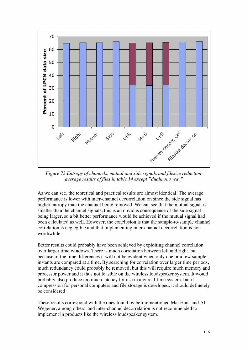
118

Figure 73 Entropy of channels, mutual and side signals and filesize reduction,average results of files in table 14 except ”dualmono.wav”

As we can see, the teoretical and practical results are almost identical. The averageperformance is lower with inter-channel decorrelation on since the side signal hashigher entropy than the channel being removed. We can see that the mutual signal issmaller than the channel signals, this is an obvious consequence of the side signalbeing larger, so a bit better performance would be achieved if the mutual signal hadbeen calculated as well. However, the conclusion is that the sample-to-sample channelcorrelation is neglegible and that implementing inter-channel decorrelation is notworthwhile.

Better results could probably have been achieved by exploiting channel correlationover larger time windows. There is much correlation between left and right, butbecause of the time differences it will not be evident when only one or a few sampleinstants are compared at a time. By searching for correlation over larger time periods,much redundancy could probably be removed, but this will require much memory andprocessor power and it thus not feasible on the wireless loudspeaker system. It wouldprobably also produce too much latency for use in any real-time system, but ifcompression for personal computers and file storage is developed, it should definetelybe considered.

These results correspond with the ones found by beforementioned Mat Hans and AlWegener, among others, and inter-channel decorrelation is not recommended toimplement in products like the wireless loudspeaker system.

119

5.5 Final algorithm proposal and benchmark

As seen in the previous segments, a large number of methods have been tested. Theresults found lays the foundation for the final algorithm proposal. Of course oneshould always keep in mind that the target application is an embedded real-timesystem. Thus, some of the demands include:

- Good worst-case as well as average performance.- Low complexity- Non-variable or low-variable computational load. Since the algorithm

operates in a real-time, low-memory system, it should be able process dataat a constant speed, thus there is not room for heavy computations even ifthey’re done rarely.

Based on these requirements, some conclusions have been drawn:

- Pod-encoding is preferred over Rice-encoding since the worst-caseperformance is much, much better.

- The iPod encoding is discarded since the overflow values are low, even ifk is calculated quite rarely.

- The predictor should not be of higher order than 2, since increasing theorder beyond this gives very little performance increase.

- The framewise polynomal approximation adds too much complexity, andcalculating k more rarely somewhat compromises it’s performance. Inaddition to several continuous accumulations one will also get a significantprocessor load increase at the start of each frame, which a real-time systemrunning ”on the edge” might not be able to handle.

- The 1st and 2nd order samplewise polynomal approximation is interesting,but the comparison and selection done for each sample adds complexity tothe algorithm. However, if the extra processor power is available, it is in areal-time system preferable to a framewise polynomal approximation orhigher-order fixed predictors.

- Inter-channel decorrelation is not worthwile to implement, since the gainon most recordings is non-existent or very limited.

Based on these criteria, a second-order fixed predictor with Pod-encoding, nochannel-decorrelation and a sample-wise computation of k is considered the bestcompromise22. Implementation in the MCU will finally determine if this is indeedfeasible and if there is any resources left over. If so, these are probably best spentimplementing a sample-wise polynomal approximation.

The suggested algorithm is finally tested for performance against the compressionapplication Carbon Shorten 1.1a for Macintosh. Shorten is considered one of the bestcompression algorithms and both Carbon Shorten and Shorten for Windows areamongst the most popular lossless compression utilities for their respective platforms.It is thus very relevant as a benchmark for comparison. Shorten is a highly developed

22 It might be that using the same k within a frame is the best option when it comes to implementationof the WLS, see the implementation considerations chapter for details.

120

scheme based on a higher-order polynomal approximation and Rice-encoding and willtherefore presumably give a better compression ratio than the much simpler algorithmdevised for our purpose. The point of the comparison is to see how close we get to themore sophisticated algorithm in terms of compression ratio with just a second orderpredictor and the Pod-coding. The comparison was done using all the files in table 18(the six mono test files) and table 30 (the six stereo test files).

Figure 74 Performance evaluation, Shorten vs. suggested algorithm for WLS

As we can see, there is as expected a performance gap to Shorten, but only bybetween two and five percent. This again shows that even a very simple predictorperforms surprisingly well and that the encoding is not significantly less efficient thanthe more advanced one used in the benchmark. Given the simplicity of the proposedalgorithm, this result is very satisfying indeed. Also, the proposed algorithm wascompiled as a single run using SDCC. The results indicates a 300-400 instructions persample complexity, depending on the input signal. This is within the capabilities ofthe MCU, but definetely on the limit, as data handling must be done simultaneously.However, if the code is optimized and, if necessary, written in assembly, it should befeasible to implement the proposed lossless compression algorithm in the WLS.

121

5.6 Lossy mode

As mentioned before, the wireless loudspeaker system has to include some sort oflossy mode if the compression ratio over a period of time does not manage to meet therequirement set by the 1Mbps transfer rate of the transceiver. The data will need to bebuffered in the MCU memory and if the buffer is about to be filled up (if more data isbeing sent from the encoder than the CC2400 is able to transmit) the lossy mode mustbe engaged. It must stay ”on” for a short while until the buffer is empty again.

The time period the lossy-mode is on will be very short, a few ms at most, but on fileswith low compressabillity it will be used quite often. It is still unlikely to be audible,but a lossy-mode scheme has to be used which does not compromise performance toomuch, to minimize the probability of perceptible degradation.

To be able to realize this, the data must be split into frames. A header is needed to tellthe decoder if the frame is encoded in lossless or lossy mode. The frame should beshort enough to not minimize distortion audability, but long enough so the headerdoes not give too much overhead.

Three different schemes for the lossy mode were considered. A model of the systemwas written in C so listening tests and measurements could be made. The threealternatives are:

- If the data rate is too high, employ a fixed-wordlength lossy compressionscheme. Then revert to lossless.

- If the output data rate is too high, remove a number of LSBs from the datain the frame to compensate.

- If the output data rate is too high, send some samples in mono tocompensate.

If we consider the first method, some kind of low-complexity lossy encoding must beemployed, probably µ-law, iLaw or an eqivalent. However, as shown earlier, each ofthese methods will, unless they are very adaptive, give low noise on low-level signalsand high noise for high-level signals, often higher than an LPCM quantization to thesame number of bits. Of course, the lossless encoding will produce the longest outputwords when the signal is loud, i.e. at the same time as the lossy compression performsbadly. Thus, alternative 2, to remove some LSBs when the bitrate is too high, willalmost certanly give a better result than, and also be much simpler than, moving tosome special lossy encoding scheme. Thus, this option is discarded. The other two areevaluated in the following subchapters.

122

5.6.1 LSB-removal lossy-mode

When the data rate from the lossless encoding is too high it is likely that the signal isloud. Removing one or a few LSBs when the signal is loud is not very perceptible, ifit is done over short periods of time, even less so. Unlike for instance µ-law lossyencoding, a hybrid scheme like this will cause loss only when the bitrate is too high totransfer (as shown earlier, µ-law gives high dynamic range, but the instantaneousquantization error is just (n-4) bits below the sample value for a n-bit encoding).

Note that requantization should ideally be combined with dithering to avoiddistortion. Dithering has been used during testing, but can be left out if the MCU doesnot have the available resources. Since the number of bits removed is quite small, thedistortion is unlikely to degrade audio quality significantly.

The frame header will need to tell the decoder two things. First, it needs to knowwhether or not the frame itself is encoded in lossy or lossless mode. Secondly, it willneed to know how many bits are removed from the samples in the frame. Since thedata input is 16 bits/sample and the decoder output is around 10 bits/sample, thenumber of LSBs needed to be chopped off can be represented with three bits.Obviously, the zero will tell the decoder that no LSBs are chopped off, which is thesame as lossless transmission, and a separate indicator for this is not needed. Oneshould note that if k is not calculated for every sample, the wordlength can increasefor some samples where k is way off. So if k is calculated rarely some frames can belarge and one might want to increase the number of bits in the header to accommodatethis. Since a sample-wise calculation of k is suggested for this system, a three-bitheader is used during testing.

During testing, a frame-size of 64 samples was used. The MCU has 2kB RAM andcan thus hold two frames, the uncompressed input frame and the compressed outputframe. Since the application is in real-time it was also important to develop a schemewhich is causal. The result was a low-complexity algorithm for employing lossy-mode: During decompression of frame N, the output data length in words is counted.If frame N is larger than a threshold, corresponding to 1Mbps, LSBs are removedwhen reading frame N+1. The number of LSBs removed always correspond to theovershoot from the length of frame N relative to the threshold. Thus the averageoutput datarate will always converge towards 1Mbps. There are 64 samples in eachframe and the desired output data rate was set to 10 bits per sample. The threshold isthen:

Eq. 38 Threshold = 64s !10bits / s = 640bits

And the number of LSBs removed from a given frame is

Eq. 39 LSB_ rem =BOUT ! 640

64

123

Where BOUT is the number of bits produced when decompressing the previous frame.When mono files are read, the bitrate is already below 1Mbps and no lossy-mode isemployed.

Figure 75 Algorithm for LSB-removal lossy mode

The lossy-mode was tested on several files and very little if any degradation of audioquality was detected. Figure 76 shows the performance on a 30s excerpt of”modernlive.wav”, a file of normal loudness. The performance is also compared tothe iLaw codec and the LAME MP3 codec at 192kbps.

124

Figure 76 Lossy-mode performance, "modernlive.wav", 30s excerpt, left channel

As we can see, the error clearly follows the frames. For many frames no bits areremoved, while for a few others up to four bits are removed. The vast majorityhowever, are between zero and two. The measured results in numbers are shown intable 32.

Table 32 Lossy-mode performanceLossy-mode SER Max absolute errorLossless with LSB-removal 88.5dB 0.00023ILaw 56.6dB 0.0043MP3, 192kbps 62.1dB 0.0024

As we can see, the loss measured in numbers is a lot better than for iLaw or MP3.This was not unexpected, as listening tests showed no audible degradation. Figure 76also shows that for most frames, zero or one LSB is removed, two for quite a few,while there in some rare instances are three to four removed. But this is in very loudparts of the track and also on high-frequency signals (due to the prediction), and doesnot appear to be audible. The lossy-modus as suggested here works very well.

125

5.6.2 Mono samples lossy-mode

The mono mode lossy algorithm developed is very similar to the LSB-removalalgorithm. It checks the output length of frame N. Then, if it is too long, it sends somesamples in frame N+1 in mono to compensate for the overshoot. The threshold iscalculated in the same way as with the LSB-removal. Since 16 bits are saved for eachsample sent in mono, the number of mono samples for frame N will be

Eq. 40 SMONO =BOUT ! 640

16

Where SMONO is the number of samples in frame N+1 to be sent in mono and BOUT isthe number of bits used in frame N. Thus, the output bitrate will average at 640 bitsper frame or 10 bits per sample. The algorihm is the same as shown in figure 75,except that SMONO is calculated instead of lsb_rem and mono samples are sent insteadof LSBs removed. When in mono-mode only the left channel is sent and the decodercopies it to both left and right after decompressing.

During testing, it soon became evident that the mono samples lossy-mode hadproblems that could not be solved without significantly compromising performance.For most frames, the right channel will toggle between being itself and being a copyof the left. Since this happens twice for each frame (when the lossy-mode is engaged)and the frames are 64 samples, the right channel will toggle it’s mode about 1,400times per second. This introduces very audible high frequency distortion. To confirmthat this was not an implementation issue, a very simple program converting a fixednumber of samples per frame to mono, without any compression or signal processing,was written. This produced the same result. The only way to avoid this distortion wasto force the mono-mode to be on for quite long periods each time, at least five to tenthousand samples (so the toggling rate is below any audible frequency). And eventhen it was easy to hear the audio going from stereo to mono and back again, thesoundstaging was almost rendered unrecognisable.

126

Figure 77 Spectrum with mono-mode, 64-sample frames, ”modernlive.wav”, 30sexcerpt.

As figure 77 shows, the HF noise level added to the right channel is significant andthe result is not by any means of high-fidelity standard. Since the LSB-removal lossymode gave excellent results, this is a no-brainer. The mono-samples lossy-mode isdiscarded.

Appendix 6 includes source-code for an evaluation program where LSB-removal ormono-mode can be selected by the user and tested. A mono-mode test-only (withoutencoding or decoding) can also be tested.

127

6 WLS Implementation ConsiderationsAs mentioned in the introduction, delays in design and manufacturing of the hardwaremade it impossible to do a full implementation before the thesis deadline. This isdetailed in the project review. But even so, algorithm design has consistently beendone with MCU implementation in mind. As a result of this, some optimizationsuggestions and general considerations will be presented as well as the work actuallydone with the hardware.

6.1 MCU implementation considerations

6.1.1 Wrap-around arithmetic

As mentioned in the lossless compression theory chapter, the output from theprediction filter is quantized to 16-bits precision. This makes the predictor slightlynonlinear, but the effect it has on the performance is neglible. Since the samequantization is done in the decoder’s filter as well, the system will of course outputthe same sample values it received and will still be completely lossless.

The residual being sent is the difference between the real value and the predictedvalue. Since both of these are 16-bit in length, the residual can, although it is higlyunlikely, be a 17-bit value23. In a powerful computer or DSP, which uses 32- or 64-bitinstructions, this is not a problem. In a 16- or 8-bit MCU however, the requirement tohandle 17-bit values instead of 16-bit will give a significant performance reduction.Every operation will have to use a significantly higher number of instructions.

But this problem can be avoided with wrap-around arithmetic. When the arithmeticonly includes summation and differenciation and the operations in the decoder areinverse of the ones in the encoder, using a 16-bit variable for the residual will not be aproblem, even if it’s value overflows. This is easiest explained using an example.

A 16-bit two’s complement variable has the value range [-32768, 32767]. If you try togo outside these values, it will wrap around. For instance:

32,767 0111 1111 1111 1111+ 1 0000 0000 0000 0001= -32,768 1000 0000 0000 0000or

-32,768 1000 0000 0000 0000- 2 0000 0000 0000 0010= 32,766 0111 1111 1111 1101

23 For the residual to use 17-bit, the difference between the real and predicted value must be more than±32,767. This rate of change is very unlikely to occur in music signals. If for instance a first orderpredictor is to give such a residual, the signal must be at almost 0dBfs (full level) and close to 20kHz,no normal recording has such an output level at those frequencies. For a higher order predictor it iseven more unlikely.

128

If we use a first order predictor and the last value x[n-1] was 19,000 and the currentvalue x[n] is –32,000, the residual, x[n]-x[n-1], will be –51,000. This is outside thevalue range and the residual will wrap around to 14,536. The decoder now has the lastsample value 19,000 and receives a residual of 14,536. In the decoder the samplevalue is of course found by adding the residual or difference to the last value, whichgives 19,000+14,536 = 33,536. This is outside the range and will again wrap aroundto –32,000, the correct value. As long as the encoder and decoder do the sameoperations, this is not a problem.

It should be noted that the wrap-around process will affect the compression, since adifferent value is compressed. However, one must remember that this is an event thatis very unlikely to happen, the probability of the prediction residual being outside the16-bit value range is almost non-existent. Thus the practical compression ratio willnot be affected and by restricting oneself to 16-bit values, significant hardwareresources are saved.

6.1.2 Look-up tables

Generally, shift operations are much slower in a MCU than in a computer processor.While a P4 or G4 can shift many bits at a time, the MCU can shift only one bit perinstruction. To avoid extensive shifting, some look-up tabels should be used. Forinstance, if the application is to check the sign bit, one can do this in two ways. For an8-bit signed variable it can be done by either

if(variable>>7) ….;

or by

if(variable&0x80) ….;

clearly, alternative two is much faster. If bit 8 is to be set one can likewise use

variable=variable|0x80;

The easiest way to handle single bits is to use a bit-table:

char bittable[8] = 0x80, 0x40, 0x20, 0x10, 0x08, 0x04, 0x02, 0x01;

Then we can use bittable[i] to either check or assign bit i in any variable. For 16-bitvariables the bit-table should of course start with 0x8000 and end with 0x0001. This isdone throughout the code.

Look-up tables should also where possible be used to replace for-loops, for instancewhen finding variables dependant on other variables. For instance, finding the

129

exponent in the µ-law encoder (the number of zeros before the leftmost ’1’ in themagnitude) is done by

value = sample<<1;for (exp=7;exp>0;exp--) if(value&0x8000) break; value = value<<1;

This can easily be replaced with a table as shown in the source-code in appendix 6.Static look-up tables like this can be included in the program memory rather than theRAM, and will thus not affect the systems memory resources (assuming that there isenough program memory, of course).

6.2 RF-link implementation considerations

6.2.1 Packet handling

The RF-link for the wireless loudspeaker system is realized with the Chipcon CC2400RF-transceiver. The CC2400 features hardware packet handling support to allowflexible and robust data transfer without stealing resources from the system. Theparameters of a packet is identified through a packet and a sync word. To avoidmultiple headers within a packet, it would therefore be smart to set the packet sizeidentical to the frame size. The suggested frame size from the lossy modus tests is at64 samples.

Eq. 41 Packet size = frame size

The packet format is shown in figure 78.

Figure 78 Chipcon CC2400 packet format [reference 22]

The ”data field” would in our case then start with the frame header and also containthe compressed audio data for the next 64 samples. The optional 8/10 coding in thefigure is an encoding of the data (IBM 8B/10B encoding scheme, see reference 22)that is in some applications used for spectral properties and error detection. Howeverit reduces the data rate to 80% of the original 1Mbps. In the WLS 8/10 coding is notconsidered necessary. However, CRC (cyclic redundancy check) should be included

130

to avoid noise corrupting the data too much. As seen in figure 78, CRC adds anoverhead of 16 bits per frame.

6.2.2 Transmission or calculation of k ?In the test applications, the Pod-parameter k is calculated for each sample in both thedecoder and the encoder using the same formula. This means no encoding parametersmust be transmitted and also gives the most symmetric codec (encoder and decoder ofabout the same complexity). However, if data corruption in the transfer occurs, the kcalculation in the decoder might not work as intended. Tests done on the compressedfile showed that changing some of the data content in the compressed file could havecatastrophic consequenses for the calculation of k, and that it might well freeze theapplication. During implementation, it should be considered if k should be sent withthe compressed data rather than being calculated in the decoder. The parameter k cantake any value from 0 to 15 and would thus generate an overhead of 4 bits. It is thenobvious that a new k cannot be calculated for each sample, rather for each frame so itcould be included in the same header. As tables 19 and 20 show, the negative effectthis has on compression ratio is very limitied, within a few tenths of a percent. Inaddition, k would add a minimal overhead of 4 bits per frame. This should be testedduring implementation, but the proposed frame would then be like shown in figure 79.

Figure 79 Proposed frame for WLS-implementation with transfer of frame-static k

When all the decoder parameters are transferred instead of being calculated, theconsequences of transmission errors are likely to be much smaller. Also, errors willnot be able to accumulate, at least not from one frame to the next.

6.2.3 Lost packet handling

Even though CRC allows you to detect and handle corrupted packets, it might happenthat entire packets are lost. This can be due to very high noise levels or interferencefrom another ISM-unit. To minimize the latter, the transmitter should do frequency-hopping (FH) from packet to packet. A frequency table must then be defined and thefrequency information added to the packet header24. Also, the compressed packetaudio data (see figure 79) should contain two original sample values (rather thanprediction errors) to allow the second order predictor to get back on track in case theprevious packet is lost.

Even so, packets will be lost. This can be handeled by either repeating the last packetor putting out silence. 64 samples correspond to 0.73ms of audio for a stereo signalsampled at fS = 44,100hz, the question is if occasional periods of silence with this

24 For details on frequency hopping the reader is referred to Chipcon Application Note AN24

131

length is audible at all and if so, will a repetition of the previous frame instead ofsilence give better or worse sound.

A program that emulated the loss of frames was written to test the audability andcompare the alternatives. The source-code is given in appendix 6. The program letsthe user select the packet length in samples, how often packets are lost (a fixed”loose-interval”, where a value of 1,000 means that 1,000 packets are sent for eachtime a loss happens), how many successive packets are lost and whether silence or arepetition of the last packet should be done to compensate.

It soon became evident that when only one packet was lost at a time, the two methodsof handling it sounded more or less identical. A 64-sample packet is just 0.7ms ofaudio, and in both cases the loss of a single packet sounded like a small ”tick”.Differences were not heard until several successive packets were dropped. A blindtest using five different audio files was set up to see how many packets had to be lostbefore a difference between the two methods could be identified, and when it could,which alternative was preferred25.

0

1

2

3

4

5

6

1 2 3 4 5 6 7 8 9 10 11 12 13 14 15 16 17 18 19 20

Number of successive packets lost

Nu

mb

er

of

au

dio

fil

es

for

wh

ich

dif

fere

nce

w

as

au

dib

le

Figure 80 Left: Audibility of difference between method 1 (silence) and 2 (repitition),1,000 packet "loose interval", 64 sample packet.

25 For information on how to set up a scientifically credible blind test, the reader is recommended thewebside of The ABX-Company, http://www.pcavtech.com/abx/index.htm

132

As we can see, 5 successive packets (3.6ms) must be lost before the differencebetween the two metods is audible on a majority of the files. When many packets arelost they sound different. Which leads to the question of which one which one ispreferable.

0

10

20

30

40

50

60

70

80

Silence Repetition

Peferred alternative

Figure 81 Preferred lost packet handling method

Of the 75 occasions for which a difference was detected, silence was preferred in 72.It should be noted that when more than 8-10 successive frames were lost the listenercould easily identify whether silence or repetition was used and knew which one he”voted for”. The evaluation in figure 81 is thus highly subjective. Nevertheless, thedistortion-like effect caused by repeating a packet several times was perceived asworse than moments of silence.

When listening to what rate of packet loss could be tolerated, the loss in audio qualitywas characterized as ”significant” when the ”loss-interval” was less than 1,000-1,500(i.e. more than one packet loss per second). When below 300-500 it was characterizedas ”annoying”.

The conclusions from the test is that a packet loss of less than one per second can betolerated and that inserting silence is preferable when packet loss happens. Insertingsilence should also be easier to implement in the WLS as no extra buffering orcalculations are required.

133

134

Part 3

- Summary –

Engineering for the sake of music;the Fender Stratocaster of late guitar extraordinare Stevie Ray Vaughan (1954-1990)

135

7 Project ReviewIn this part of the thesis a review of the project itself and the work done will bepresented.

The Wireless Loudspeaker System was a project initiated by Norwegiansemiconductor company Chipcon to develop a demonstration platform for theirCC2400 RF-transceiver. The requirements for the design was that it should be low-cost, relatively simple and implemented using only standard hardware, i.e.microcontroller, logic circuits and the RF-chip, no dedicated DSPs, FPGAs oranything like that.

From the beginning the goal of the thesis was to evaluate and find a suitable low-complexity and high-fidelity compression algorithm and implement this using a MCUdemonstration board strapped to the CC2400EWB. However it soon became apparentthat no such demonstration boards had the necessary peripherals. Since Chipconwanted a reference design anyway we agreed on including hardware design as part ofthe thesis. The WLS was thus designed from scratch.

To design the WLS proved to be more work than anticipated; as shown earlier in thisthesis, a custom communications system using logic devices had to be developed. Asa consequense, the hardware design phase took almost a month more than plannedand the complete and verified circuit design was delivered to Chipcon formanufacturing in mid March instead of mid Febuary as intended.

The plan was then for me to do compression algorithm research using my computerwhile waiting for the finished PCB. I was supposed to receive it soon after easter anduse the last four to six weeks on implementation. However, there were also significantdelays in the manufacturing of the circuit. Since this was beyond my control I usedthe time to do a much more extensive research and development on compression thanfirst planned and both a custom lossless and a custom lossy algorithm has beenproposed. The finished WLS-hardware would not leave production before the thesisdeadline and an implementation was thus not possitble to achieve before finishing thethesis.

However, although I recognise implementation as both an important and instructiveprocess, I do not believe that the academical reward of the project was compromisedbecause of these delays. The extra effort put into audio compression gave valuableinsight into a field of which I have great interest and it also produced some very goodresults, both for the lossy and lossless part. Also, desiging the hardware proved to bevery educational. I learned a lot about embedded systems design as well as gaininginsight into how the business works; how a design process is handeled, howverification and frequent reviews are of utter importance and generally how toadministrate a fairly extensive project.

136

8 SummaryThis thesis convers the work done developing the Wireless Loudspeaker System. Ithas been my intention to make it a complete document, and I have therefore presenteda theory section so the reader is able to understand the work and the results evenwithout looking up in the references. The theory that is not directly related to thethesis main focus, but still has been relevant to the development process, is presentedin appendixes 1 and 2. This covers the different formats and protocols used in thesystem (appendix 1) as well as general data conversion theory (appendix 2). The otherappendixes include the circuit, the PCB-design, the equipement used as well as thesource-code.

Regarding the source-code, only the most relevant applications are included. Duringthe project over 50 different versions of various compression algorithms werecompiled and tested. To include all these would make the report much to extensive.The source-code in the appendix includes DPCM, ADPCM, µ-law, iLaw, a Rice-/Pod/iPod entropy coder and decoder, a lossless codec with selectable prediction, ahybrid lossy/lossless codec and the frame drop test algorithm. In addition the MatLabscripts referred to in the thesis are also given in appendix 7.

The practical part of the thesis documents the work done, from finding the appropriatecomponents to hardware and software design. The hardware documentation ends in afinished design, while the software documentation, due to the implementation notbeing done, ends with considerations and suggestions. Based on measurements andsubjective listening tests, compared to an assessment of computational complexityand MCU implementation feasibility, conclusions are drawn and algorithmssuggested. For the lossy option, a custom made iLaw algorithm is proposed whichfeatures high performance (comparable to 128kbps MP3) and very low complexity(estimated at around 250 instructions per sample in an 8-bit MCU). The losslessalgorithm suggested uses a second order predictor and Pod-coding. It featurescompression ratios within a few percent of the much-recognised home computerapplication Shorten, a lossy-mode for constant bitrate and an encoding with very goodworst-case performance to ensure minimum influence from this lossy-mode.Complexity tests show it should be feasible to implement in an MCU-based system.

To summarize, I think this project, despite it not being completely finished within thethesis deadline, has been an academical success. I have learned a lot about audiocompression, digital signal processing, general programming and embedded systemsand hardware design. These are all important areas for an engineer to master and Iconsider the gained knowledge to be extremely valuable. Also, much practicalengineering work has been done, which I find very rewarding since it has made mebetter equipped to face the challenges that meet me outside the university.

137

9 References1. ”Data Compression Basics”, Slides, EECC6942. ”Optimization of Digital Audio for Internet Transmission”, Ph.d Thesis

Mathieu Claude Hans3. Windrow, B. et.al.: ”Stationary and non-stationary learning

characteristics of LMS adaptive filter.” Proc IEEE, 19764. G. Mathew et.al: ”Computationally simple ADPCM based on exponential

power estimator” Proc. IEEE, 19925. Monkey’s Audio theory6. T. Robinson: ”Shorten: simple lossless and near-lossless waveform

compression.”, Technical Report 156, Cambridge University, 19947. Lesson 8: Compression Basics, Computing and Software Systems lecture

notes, University of Washington Bothell8. Introduction to multimedia, Cardiff University9. Debra A. Lelewer , Daniel S. Hirschberg, “Data compression”, ACM

Computing Surveys (CSUR), v.19 n.3, p.261-296, Sept. 198710. LOCO-1: Weinberger, M, Seroussi, G, Sapiro, G: “A low-complexity,

Context-based, lossless image compression algorithm.” IEEE DataCompression Conference, 1996

11. Weinberger, M, Seroussi, G: “Modeling and low-complexity adaptivecoding for image prediction residuals”, IEEE.

12. Robin Whittle: “First Principles, Lossless compression of audio”13. Fraunhofer institute, ”MPEG-1 Layer 3 overview”.

http://www.iis.fraunhofer.de/amm/techinf/layer3/index.html14. Microsoft corp.: ”Windows Media Encoder whitepaper”

http://download.microsoft.com/download/winmediatech40/Update/2/W98NT42KMeXP/EN-US/Encoder_print.exe

15. Sony: ”ATRAC whitepaper” http://www.minidisc.org/aes_atrac.html16. Fraunhofer Institute, “MPEG-2 AAC overview”.

http://www.iis.fraunhofer.de/amm/techinf/aac/index.html17. Chipcon Application Note 126 ”Wireless Audio using CC1010”18. IMA Digital Audio Focus and Technical Working Groups:

”Recommended practices for enhancing digital audio compatibility inmultimedia systems.” rev. 3.00, October 21, 1992

19. W.M. Hartmann ”Signals, sounds and sensations”, AIP Press, 199720. R.G. Baldwin: ”Java Sound, Compressing Audio with mu-Law encoding”21. ”Vorbis-1 specification”, Xinph.org foundation,

http://www.xiph.org/ogg/vorbis/doc/Vorbis_I_spec.html22. Chipcon SmartRF CC2400 datasheet

http://www.chipcon.com/files/CC2400_Data_Sheet_1_1.pdf23. AKM AK4550 datasheet24. Texas Instruments TLV320AIC23B datasheet25. Analog Devices AD1892 datasheet

http://www.analog.com/UploadedFiles/Data_Sheets/294553517AD1892_0.pdf

26. Crystal Semiconductors CS8420 datasheethttp://www.cirrus.com/en/pubs/proDatasheet/CS8420-5.pdf

138

27. AKM AK4122 datasheet preliminarywww.akm.com/datasheets/ak4122.pdf

28. Crystal Semiconductors CS8416 datasheethttp://www.cirrus.com/en/pubs/proDatasheet/CS8416-4.pdf

29. Wegener, Albert: ”MUSICompress: Lossless, Low-MIPS AudioCompression in Software and Hardware.”Soundspace Audio, 1997

30. Atmel AVR Mega169 datasheethttp://www.atmel.com/dyn/resources/prod_documents/doc2514.pdf

31. Atmel AVR Mega32 datasheethttp://www.atmel.com/dyn/resources/prod_documents/doc2503.pdf

32. Texas Instruments MSP430F1481 datasheet. http://www-s.ti.com/sc/ds/msp430f1481.pdf

33. Motorola DSP56F801 datasheet http://e-www.motorola.com/files/dsp/doc/data_sheet/DSP56F801.pdf

34. Motorola DSP56800-family reference manual http://e-www.motorola.com/files/dsp/doc/ref_manual/DSP56800FM.pdf

35. Hitachi/Rensas R8C/10 datasheethttp://www.eu.renesas.com/documents/mpumcu/pdf/r8c10ds.pdf

36. Silicon Laboratories C8051F005 datasheethttp://www.silabs.com/products/pdf/C8051F0xxRev1_7.pdf

37. 74HC4094N datasheet38. 74HC166N datasheet39. 74HC4020 datasheet40. Kernighan, Brian W. & Ritchie, Dennis M. : ”The C Programming

Language”, 2nd edition, Prentice Hall 1989.

139

140

APPENDIXES

141

142

Appendix 1. Data Formats

The wireless audio system must both in hardware and software be compliant withseveral standard interfaces used by the various chips. The digital audio input is basedon the SP-dif (Sony/Philips digital interface format) format and is decoded with adedicated receiver. Both this receiver and the audio codec which manages the analoginputs and outputs use the I2S (Inter IC Sound) standard for communicating with othercircuits. Thus the communication between the MCU and these units must becompatible with their I2S interfaces. Finally, the communication between the MCUand the RF-chip uses the SPI (Serial Peripheral Interface) format.

In addition, the compression algorithms used in this project have been developed andtested on Mac OS-X and Windows computers. The most widespread uncompressedaudio format for computer use is the WAV-format (Waveform Audio Format), whichhas been used during testing and development. The WAV-file format is alsoexamined in the following sections.

SP-dif (Sony/Philips-data interface format)

The Sony/Philips digital interface format [reference A1-1] is a consumer version ofthe AES/EBU (Audio Engineering Society / European Broadcasting Union) formatand is given by the IEC958 standard of 1989. While AES/EBU was developed as adigital audio interface for professional use, the SP-dif is intended for home audioequipement and therefore has some changes in the data being transferred. Also, thephysical connection is unbalanced with much lower signal levels, since the cablinglength and surrounding noise levels will be much lower in a home audio system thanin a professional recording studio. The main differences between AES/EBU and SP-dif are listed in table A1-1.

Table A1- 1 SP-dif vs AES/EBU digital audio interfaces [referenceA1- 2]AES/EBU SP-dif

Cabling 110ohm shielded TP 75ohm coaxial of fiber (Toslink)Connector 3-pin XLR RCA (or BNC)Signal level 3-10V 0.5-1VModulation Biphase-mark-code Biphase-mark-codeSubcode information ASCII ID text SCMS copy protection infoMax. resolution 24-bits 20-bits (24-bits optional)

Every sample is transferred in a 32-bit subframe. The left and right channel subframesrepresents one frame. The subframes and frames are seperated with a preamble, a bit-pattern containing a biphase-coded error. This because the receiver must be able toidentify the start of a sample or a data block. Figure A1-1 shows a how the subframesand frames are built up.

143

Figure A1- 1 SP-dif subframes and frames [reference A1-1]

The different preambles have the following meaning:

- Preamble X: Tells us the subframe has data for the left channel. Thesubframe is not at the start of the data block.

- Preamble Y: Tells us the subframe has data for the right channel. Thesubframe is not at the start of a data block.

- Preamble Z: The subframe has data for the left channel and we are atthe start of a new data block.

In a subframe, the first four bits are preambles. After these, four AUX data bitsfollow. They are used to tranfer information about tracks, like name, track numberand soforth. Bit 8 to 27 contains the actual audio data, max 20-bits. If the datawordlength is 24-bits, the AUX-bits are also used for audio data. After the audio datacomes a validity-bit, a user bit, a channel status bit and a parity bit.

Figure A1- 2 The content of SP-dif subframes and data blocks [ref.A1-1].

144

As seen in figure A1-2, each data block contains 192 frames and will always startwith a left channel sample. In each frame, a total of 384 channel-status and subcode-information bits are transferred. This data information must be decoded by the SP-difreceiver as shown in figure A1-3.

Figure A1- 3 Channel status block data, SP-dif (left) and AES/EBU (right) [ref.A1-1]

Figure A1-3 also shows the difference between the SP-dif consumer format and theAES/EBU professional format. The latter does not have copyright information, but itdoes contain some other information like reliability, reference, when the data isrecorded etc. It also contains some user configurable bits like channel setup overrideand sample frequency. This information is not needed in consumer equipement, whichare meant only to playback the data, and not to alter it.

It must also be mentioned that the IEC958 standard was renamed IEC60958 in 1998and has been expanded to also carry IEC61937 datastreams. IEC61937 data cancontain multichannel sound like MPEG-2, AC3 or DTS [reference A1-2].

I2S (Inter IC Sound)

I2S (Inter IC Sound) [reference A1-3] is a bus developed by Philips for transmissionof digital audio between different chips within a system. The bus only transfers audiodata, while control and information signals are sent between the components other IO-pins. I2S is a three-wire bus with one data-connection, one bitclock-connection (toclock the bits in the serial data stream) and one word-clock or LR-clock connection(to clock the samples, left channel sample when the LR-clk is ’0’ and right channelsample when it is ’1’). The unit generating the clock signals will function as master.The audio samples are transferred as two’s complement PCM with the MSB-first.Since the MSB is transferred first, the transmitter is not dependent of knowing howmany bits the receiver can handle. If a 24-bit transmitter is connected to a 16-bitreceiver, the 8 LSBs will be ignored on reception. If a 16-bit source is connected to a24-bit receiver, the 8 LSBs will be set to zero. All timing demands in the I2S-protocol

145

are proportionate to the clock frequency, thus higher sample-rates can be allowed infuture applications.

Figure A1- 4 I2S-interface data transfer diagram [reference A1-3]

Figure A1-4 shows the I2S data transfer, where SCLK is the serial- or bit-clock whileLRCK is the left-right- or word-clock. SDTI is the data transfer pin. As shown theSCLK usually runs at 32fS or 64 fS, where fS is the sample frequency. At the formerfrequency the PCM word-length can be 16-bit, 20-bit or, in theory, up to 31-bit (or32-bit with left- og right-justification, which is explained below). However, no currentaudio equipement exceeds 24-bit resolution26. In a 16-bit or less system, the SCLKusually runs at 32 fS, easing the timing requirements. The LRCLK runs at the samplefrequency fS.

One should also notice that the sample MSB comes one BCLK-cycle after a transitionon LRCK. This is how the I2S-standard is specified and is often referred to as I2S-justification. However, most audio components also allow for left-justification (theMSB comes when the LRCK toggles, one cycle earlier than I2S-justification) or right-justification (the LSB comes at the last BCLK cycle before LRCK toggles) of the datastream. One should notice that right-justification as mentioned demands the samewordlength on transmitter and receiver.

SPI (Serial Peripheral Interface)

The SPI- (Serial Peripheral Interface) format is a four-wire synchronous, full-duplexdata transfer bus developed for low-complexity data interfacing between peripheralsin computer systems or embedded systems. It uses four wires, MOSI (Master Out,Slave In), MISO (Master In, Slave Out), SCK (Serial Clock) and NSS (Negative SlaveSelect). The active-low NSS-pin is used to select a slave device and enable data 26 Even though the digital resolution or wordlength in modern audio equipement is usually 24-bits, theeffective resolution, given by A/D- and D/A-converter linearity and system noise levels, is currentlyonly around 20-bit in state-of-the-art systems. However, a seemingly excessive wordlength (true 24-bitresolution seems impossible with todays technology) allows for more accurate digital signalprocessing, with less degradation of signal quality.

146

transfer between it and the master. The MOSI and MISO are the data lines between themaster and slave, and the SCK is used to clock the transfer. A typical SPI-system witha master (for instance a microcontroller) and three slave devices is shown in figureA1-5.

Figure A1- 5 Typical SPI system [reference A1-5]

The data on both the MOSI and MISO pin is transferred MSB-first. A SPI-pin alsoplaces the MISO-pin in tristate (high-impedance) when it is not selected, so it’s outputdoes not load the bus.

WAV (Waveform Audio Format)

The WAV (Waveform Audio) format [reference A1-6] is a proprietary Microsoftformat and part of the RIFF family (Microsoft media-format family). It stores raw,uncompressed audio samples as PCM-values and can be used with any normalsample-rate or wordlength. The number of channels can be one (mono), where thesamples are stored successively, or two (stereo) where every other sample is a left- orright-channel sample. In computer audio, WAV has become the standard for storinguncompressed digital audio. Even though Apple has it’s own format, AIFF, almostany audio software and all computers, including all Macintosh models, can read andwrite WAV-files.

The WAV-format is very simple. In addition to raw audio data, it consists of a headerwhich identifies it as a WAV-file. The header also tells the application if it’s mono orstereo, what the the sample rate and resolution (wordlength) is, the filesize and alsosome other information. The 44-byte header is stored at the start of the file and isfollowed by the audio data like shown in figure A1-6

147

Figure A1- 6 WAV audio file header [reference A1-6]

The header is often reffered to as consisting of three ”chunks” of information. Theseare identified as follows:

1. RIFF Chunka. Byte 0-3: ”RIFF” (ASCII characters); identifies the file as a RIFF-file.b. Byte 4-7: Total length of package to follow (binary, little endian).c. Byte 8-11: ”WAVE” (ASCII characters); identifies the file as a WAV-

file.2. FORMAT Chunk

a. Byte 0-3: ”fmt_” (ASCII characters); identifies the start of the formatchunk.

b. Byte 4-7: Length of format chunk (binary, always 0x10).c. Byte 8-9: Always 0x10.d. Byte 10-11: Number of channels (1 – mono, 2 – stereo).e. Byte 12-15: Sample rate (binary, in Hz).f. Byte 16-19: Bytes per second (samplerate"#channels"bitspersample/8).g. Byte 20-21: Bytes per sample (align: 1 = 8-bit mono, 2 = 8-bit stereo

or 16-bit mono etc.).h. Byte 22-23: Bits per sample (sw).

3. DATA Chunka. Byte 0-3: ”data” (ASCII characters); identifies start of the data chunk.b. Byte 4-7: Length of data to follow.c. Byte 5…: Audio data.

The header can also in some cases contain other chunks that specifies index marks,textual description of the sound etc., but these are not relevant for this project, so theywill not be investigated further in this report. The interested reader is recommendedreference A1-6, ”The File Format Handbook” by Gunter Born.

References:A1-1: IEC 958 ”Digital Audio Interface” whitepaper, European Broadcasting

Union, 1989.A1-2: ”About SP-dif”, Tomi EngdahlA1-3: ”The Inter IC Sound” whitepaper, Philips corp.A1-4: AKM 4553 datasheet, AK corp.A1-5: Silicon Laboratories C8051F00x datasheet rev. 1.7A1-6: ”The File Format Handbook”, Gunter Born, 1995, ITP-Boston

148

Appendix 2. Data Converter FundamentalsAs mentioned in the theory chapter, digitizing an audio signal involves two processes,sampling and quantization. When sampling, the amplitude of the signal is measured ata fixed sampling interval T. The interval is usually described with the samplingfrequency fS=1/T. Sampling converts the signal from continous time to discrete time.When quantizing the amplitude is assigned to a number of discrete values between 2-B

and 2B where B is the number of bits in the digital representation. This is, aspreviously explained, LPCM code. The result is a discrete-time and discrete-amplitude digital signal. The illustration from figure 2 is repeated for clarity.

Figure A2- 1 Sampling and quantization of audio signal

A sampled discrete time sinusiod can may be expressed as

Eq. A2- 1 x[n]= A ! cos("n +#) ,+<n<+ ;[reference A2-1]

Where n is an integer variable (the sample instant) and ! is the sample frequencygiven by ,"T. , is the signal’s ”analog” frequency in radians per second (, = 2-fwhere f is the frequency in hertz) and T is the sample period. By definition a discrete-time signal x[n] is periodic only if it’s frequency ! is a rational number, that is:

Eq. A2- 2 x[n+N] = x[n] , for all n ;[reference A2-1]

The smallest period N for which this is true is called the fundamental period. It caneasily be shown that for the discrete time sinusiod the fundamental period is 2-because:

149

Eq. A2- 3 cos[(! + 2" )n +#] = cos(!n + 2"n +#) = cos(!n +#) ;[reference A2-1]

This means that every discrete sinusoidal sequence where ! k = ! + 2k" areindistinguishable when [!" # $ # " ] . On the other hand the sequence of any twosinusoids with frequency in the range [!" # $ # " ] are distinct. The frequenciesoutside this range is thus described as aliases of the distinct frequencies. Since! =!T =! / fs it becomes apparent that:

Eq. A2- 4 !" # $ # " => ! " #$fs# " or ! 1

2"ffs"12

;[reference A2-1]

must be fulfilled for any analog signal to be given a distinct sampled sequence. Thesignal must be below half the sampling frequency. This is known as the Nyquistfrequency or Shannon’s sampling theorem after Harry Nyquist and Claude Shannonwho derived it. An attempt to sample anything outside the Nyquist frequency will asequation A1-3 indicates produce an unwanted signal of which the input is an alias. Toavoid this, filtering must be performed before AD-conversion. Likewise, filtering isdone after DA-conversion to avoid aliases as well as the original spectrum beingreproduced from the digital sequence. Both pre-ADC and post-DAC filtering isreferred to as antialias-filtering og just antialiasing.

The other fundamental limitation in digital signals is the resolution, given by thequantization. For a B-bit digital quantization the smallest distance, the quantizationstep Q, is given by R/2B where R is the signal range (see figure A1-1). A roundofferror is subsequently made. If it is assumed to be random, it is given as a whitedistribution between:

Eq. A2- 5 !Q2" e " Q

2;[reference A2-3]

This gives a RMS-error of

Eq. A2- 6 eRMS = e2 = 1Q

e2de!Q /2

Q /2

" =Q12

;[reference A2-3]

If the signal to be quantized is a random signal distributed between 0 and R the signal-to-noise ratio (SNR) will be:

Eq. A2- 7 SNR = 20 ! logVin(RMS )eRMS

"#$

%&'= 20 ! log R / 12

Q / 12"

#$%

&'= 20 ! log(2B ) = 6.02 ! B [dB]

150

This is referred to as the ”6dB per bit rule”. For a sinusoidal input the SNR can easilybe calculated to 6.02B+1.76 dB by using the RMS-value for a sinusiod of amplitudeR/2.

However, although these are the only fundamental limitations of a signal digitized at fsand with B bits there are other nonidealities in the conversion that can compromiseperformance.

Figure A2-2 shows the transfer characteristic for an ideal 2-bit ADC and a DAC

Figure A2- 2 Transfer characteristic for ideal 2-bit ADC and DAC [ref A2-2]

The ideal ADC assigns a new value exactly at the quantization interval while the idealDAC draws a completely straight line between the sample values. In real-lifehowever, there are several factors that compromise performance:

- Offset-error: DAC: The output that occurs for the input code thatshould produce zero output. ADC: The output code for a zero voltinput level.

- Gain-error: The difference between the ideal and actual full-scale valuewhen the offset error has been reduced to zero.

- Differential nonlinearity error (DNL): the variation in analog step sizesaway from 1 LSB with the two above removed. DNL values aredefined for each digital value.

- Integral nonlinearity error (INL): The difference between the ideal andactual transfer curve when offset- and gain-error has been removed.The maximum INL is also often referred to as absolute accuracy.

151

Figure A2- 3 INL error and red. in SFDR (spurious free dynamic range) [ref A2-4]

As can be seen, these errors introduce nonlinearity or distortion. The resultingresolution is often referred to as SFDR or spurious-free dynamic range and ismeasured in dB or effective number of bits. For current state-of-the-art 24-bit DACs,the effective number of bits is in the range of 20 bits.

Another non-ideality of data conversion is jitter. Jitter occurs when there is variationin the sample period T due to inaccuracy in the systems clock signals. Jitter leads todistortion of the signal as shown in figure A2-4.

Figure A2- 4 Distortion as a consequence of jitter [ref A2-3]It can be shown that for a 16-bit system reproducing a 20kHz tone at full level, thejitter distortion will be higher than the quantization noise at >127ps jitter, and it willthus reduce the SFDR. In high-end audio applications, jitter is currently one of theperformance bottlenecks.

The final performance limitation reviewed here is granulation noise. It was previouslyassumed that the quantization noise e is random. However, for low values or a veryfew bit representation this is not the case. This can easily be understood by looking atthe output and error from a few-bit ADC.

152

Figure A2- 5 Transfer curve and error for few-bit ADC [ref A2-2]

As we can see, there is correlation between the signal and the noise, which leads to adistortion called granulation noise. The granulation noise is mostly audible at lowvolumes and sounds much more uncomfortable than straight white noise. Thereforerequantization is often done together with dithering, a process where white noise isadded to the signal before it is truncuated. The point is to decorrelate the signal andthe noise and thus substitute uncomfortable distortion with white noise. Dithering isdisplayed in figure A2-6 and the effect of it in figure A2-7.

Figure A2- 6 Dithering and quantization [ref. A2-3]

153

Figure A2- 7 The effect of dithering on a signal with amplitude 2Q [ref. A2-3]

The dither-signal is often generated by an independent random noise-source andshould then have a maximum amplitude of ! 1

2Q, 12Q"# $% . This will lead to a 3dBdecrease of SNR, but the distortion will be reduced significantly and the sonic resultis an improvement. Almost every requantization in modern hifi-circuits is done withdithering.

However, it can be shown that a random noise source as a dither generator is notideal. Using random noise is known as rectangular dither. This because the dithersignal has a rectangular probability density function (PDF). It can be shown that therectangular dither does not completely decorrelate the signal and the quantizationnoise. Triangular dither does exactly that. Realized as a convultion of two randomnoise-sources it will have a decreasing or triangular PDF. The amplitude can howeverreach ±Q and it can be shown that the nominal noise floor will increase with 4.77dBas opposed to 3dB. This is made up for by the resulting quantization noise, withtriangular dithering, having a completely uniform mean value and variance, i.e.complete decorrelation from the signal (white noise). Thus triangular dither is usuallypreferred in audio applications. Triangular dithering can digitally be realized easily bypassing the output from a random noise source through a (1-z-1) filter. The noise-source is in normally made by a pseudo-random number generator.

When quantizing an analog signal on the other hand, the dither source also has to beanalog. To generate triangular dithering with solely analog components is notpossible. Analog dithering is often realized with a gaussian PDF, since this is thesame probability distribution as for natural white noise or thermal noise. Thermal

154

noise is generated by resistance in a circuit and a ±Q gaussian dither can thus berealized with nothing more than a simple diode or resistor (diodes are normally used,to avoid loading the input). Gaussian dithering is however less ideal than triangularsince it increases the nominal noise-floor by 6dB.

Figure A2- 8 The PDF of gaussian, rectangular and triangular dither [ref. A2-3]

References:A2-1: Proakis, John et.al.: ”Digital Signal Processing, Principles, Algorithms

and Applications”, Prentice Hall 1996.A2-2: Johns, David et.al: ”Analog Integrated Circuit Design”, John Whiley

& Sons, 1992A2-3: Løkken, Ivar et.al: ”One-O digital amplifier”, bachelor thesis, HiST

2002A2-4: Løkken, Ivar: ”Delta-sigma Audio DAC for SoC applications”, project

report, NTNU 2003

155

Appendix 3. Schematics

156

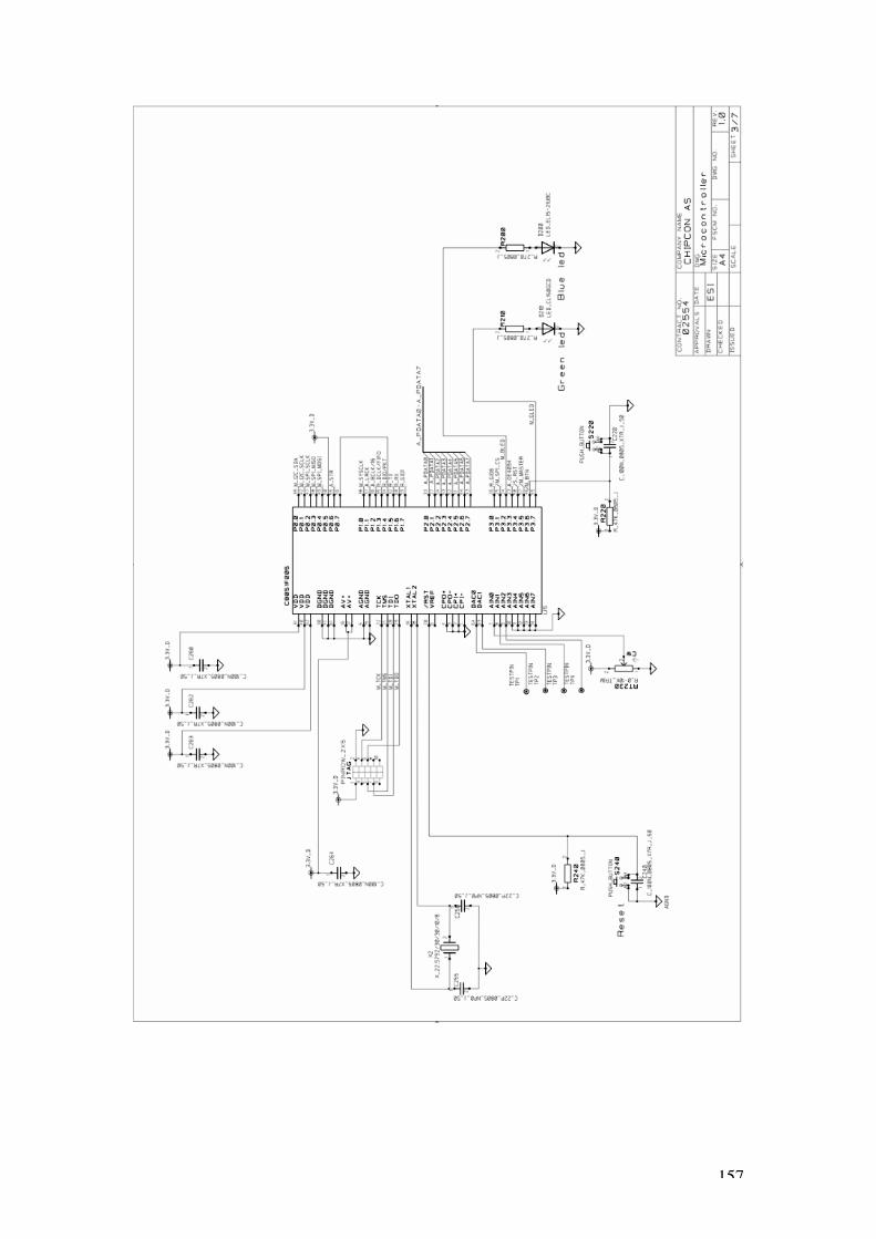
157

158

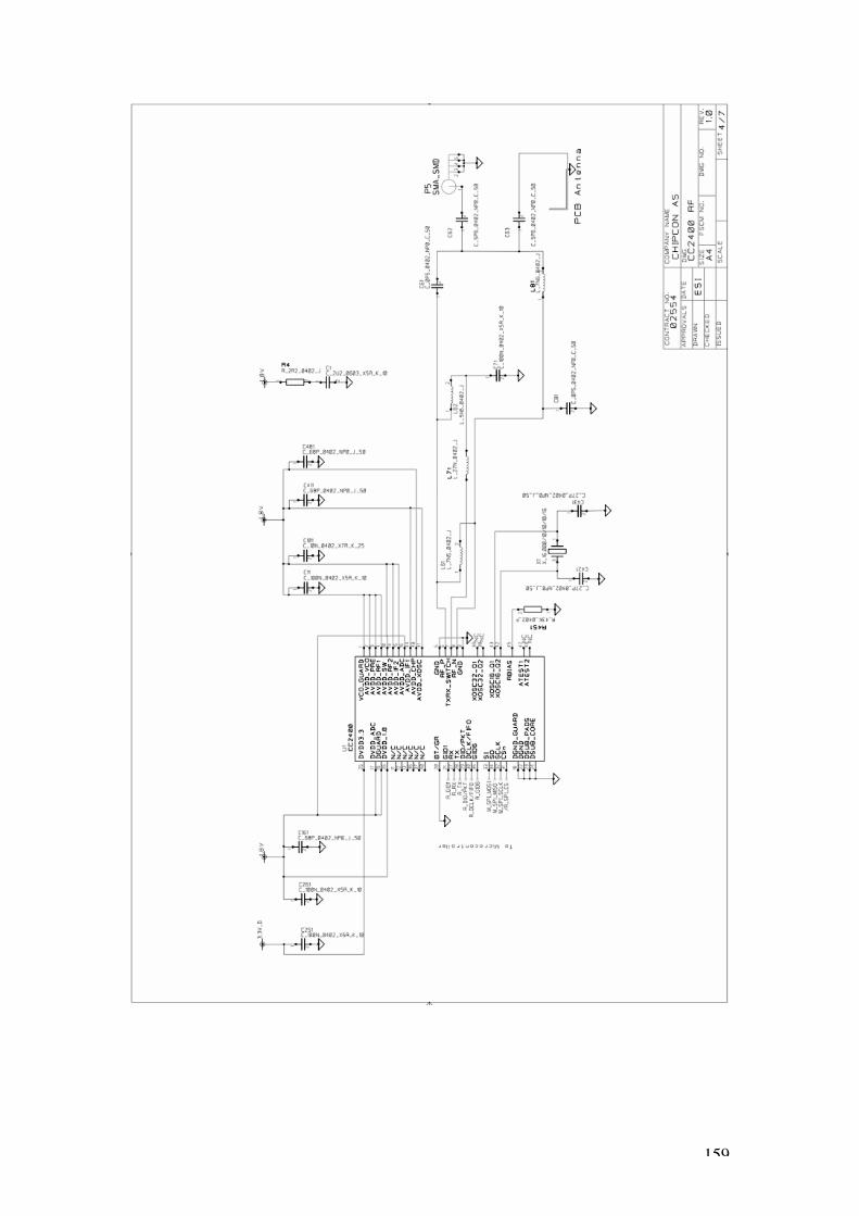
159

160

161

162

Appendix 4. Components List

163

Appendix 5. PCB-Layout

164

165

166

167

168

169

170

171

172

173

174

175

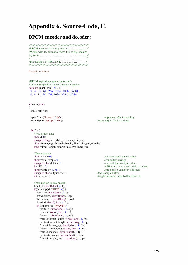
176

Appendix 6. Source-Code, C.DPCM encoder and decoder:////////////////////////////////////////////////////////////////////////////////DPCM encoder, 4:1 compression..............………..////Works with 16-bit mono WAV-file on big-endian////systems....................................…………………….////...........................................………………………..////Ivar Løkken, NTNU, 2004....................………….///////////////////////////////////////////////////////////////////////////////

#include <stdio.h>

//DPCM logarithmic quantization table//One set for positive values, one for negativestatic int quantTable[16] = 0, -4, -16, -64, -256, -1024, -4096, -16384, 0, 4, 16, 64, 256, 1024, 4096, 16384;

int main(void) FILE *fp, *op;

fp = fopen("in.wav", "rb"); //open wav-file for reading op = fopen("out.dp", "wb"); //open output-file for writing

if (fp) //wav header data char id[4]; unsigned long size, data_size, data_size_sw; short format_tag, channels, block_allign, bits_per_sample; long format_length, sample_rate, avg_bytes_sec;

//data variables short value = 0; //current input sample value short value_temp = 0; //for endian change unsigned char delta = 0; //current dpcm output value int diff = 0; //difference, actual and predicted value short valpred = 32767; //predicttion value for feedback unsigned char outputbuffer; //two-sample buffer int bufferstep; //toggle between outputbuffer fill/write

//read and write wav header fread(id, sizeof(char), 4, fp); if(!strncmp(id, "RIFF", 4)) fwrite(id, sizeof(char), 4, op); fread(&size, sizeof(long), 1, fp); fwrite(&size, sizeof(long), 1, op); fread(id, sizeof(char), 4, fp); if(!strncmp(id, "WAVE", 4)) fwrite(id, sizeof(char), 4, op); fread(id, sizeof(char), 4, fp); fwrite(id, sizeof(char), 4, op); fread(&format_length, sizeof(long), 1, fp); fwrite(&format_length, sizeof(long), 1, op); fread(&format_tag, sizeof(short), 1, fp); fwrite(&format_tag, sizeof(short), 1, op); fread(&channels, sizeof(short), 1, fp); fwrite(&channels, sizeof(short), 1, op); fread(&sample_rate, sizeof(long), 1, fp);

177

fwrite(&sample_rate, sizeof(long), 1, op); fread(&avg_bytes_sec, sizeof(long), 1, fp); fwrite(&avg_bytes_sec, sizeof(long), 1, op); fread(&block_allign, sizeof(short), 1, fp); fwrite(&block_allign, sizeof(short), 1, op); fread(&bits_per_sample, sizeof(short), 1, fp); fwrite(&bits_per_sample, sizeof(short), 1, op); fread(id, sizeof(char), 4, fp); fwrite(id, sizeof(char), 4, op); fread(&data_size, sizeof(long), 1, fp); fwrite(&data_size, sizeof(long), 1, op); else printf("Error: RIFF-file, but not a wave-file\n");

else printf("Error: not a RIFF-file\n");

//byteswapping of data_size since it is arranged with msbyte lastdata_size_sw = 0;data_size_sw = ((data_size&0x000000ff)<<24);data_size_sw = (data_size_sw|((data_size&0x0000ff00)<<8));data_size_sw = (data_size_sw|((data_size&0x00ff0000)>>8));data_size_sw = (data_size_sw|((data_size&0xff000000)>>24));printf("Data size: %d \n", data_size_sw);

// RUN COMPRESSIONfor ( ; data_size_sw>0; data_size_sw=data_size_sw-2)

// read input value and change endianfread(&value_temp, sizeof(short), 1, fp);value = 0;value = ((value_temp & 0x00ff)<<8);value = (value | ((value_temp & 0xff00)>>8));

//first order prediction (difference)diff=value-valpred;

//set signbit and work with absolute values. if (diff < 0)

diff = (-diff);delta = 0;

else delta = 8;

//find the four bit output code//(binary tree bit 2-4, first is sign bit)//Sxxx, where S is sign

//check second bitif (diff >= 256) //set second bit => S1xx delta |= 4; //check third bit if (diff >= 4096) //set third bit => S11x delta |= 2; //check fourth bit if (diff >= 16384) //S111 delta |= 1; else //third bit 0 => S10x //check fourth bit if (diff >= 1024) //S101

178

delta |= 1;

//S0xx else if (diff >= 16)

//S01x delta |= 2; if (diff >= 64)

//S011 delta |= 1;

//S00x else if (diff >= 4)

//S001 delta |= 1;

//feedback dequantized delta valpred += quantTable[delta];

//put two samples in the 8-bit output-buffer and write it to file //if bufferstep == 1; buffer = cccc0000 (c=current adpcm sample) //else: buffer = ccccpppp (c=current, p=previous) //then write it to file //bufferstep toggles - two samples in buffer before write

if (bufferstep) outputbuffer = (delta << 4) & 0xf0; else outputbuffer = (delta & 0x0f) | outputbuffer; fwrite(&outputbuffer, sizeof(char), 1, op); bufferstep = !bufferstep; //output last step, if necessary if (!bufferstep) fwrite(&outputbuffer, sizeof(char), 1, op); fclose(fp); fclose(op);

179

////////////////////////////////////////////////////////////////////////////////DPCM decoder, 4:1 compression.............………...////Works with 16-bit mono WAV-file on big-endian////systems....................................……………………..////...........................................………………………...////Ivar Løkken, NTNU, 2004....................…………..///////////////////////////////////////////////////////////////////////////////

#include <stdio.h>

//DPCM logarithmic quantization table//One set for positive values, one for negative

static int quantTable[16] = 0, -4, -16, -64, -256, -1024, -4096, -16384,0, 4, 16, 64, 256, 1024, 4096, 16384

;

int main(void) FILE *fp, *op; fp = fopen("in.dp", "rb"); //open wav-file for reading op = fopen("out.wav", "wb"); //open output-file for writing

if (fp) //wav header variables char id[4]; unsigned long size, data_size, data_size_sw; short format_tag, channels, block_allign, bits_per_sample; long format_length, sample_rate, avg_bytes_sec;

//data variables char delta = 0; //current dpcm input value int valpred = 32767; //predicted output value short valout; //ouput value for writing char inputbuffer = 0; //2-sample input buffer int bufferstep = 0; //toggle between inputbuffer/input

//read and write wavinfo fread(id, sizeof(char), 4, fp); if(!strncmp(id, "RIFF", 4)) //if it is a RIFF, continue fwrite(id, sizeof(char), 4, op); fread(&size, sizeof(long), 1, fp); fwrite(&size, sizeof(long), 1, op); fread(id, sizeof(char), 4, fp); if(!strncmp(id, "WAVE", 4)) //if it is a WAVE, continue fwrite(id, sizeof(char), 4, op); fread(id, sizeof(char), 4, fp); fwrite(id, sizeof(char), 4, op); fread(&format_length, sizeof(long), 1, fp); fwrite(&format_length, sizeof(long), 1, op); fread(&format_tag, sizeof(short), 1, fp); fwrite(&format_tag, sizeof(short), 1, op); fread(&channels, sizeof(short), 1, fp); fwrite(&channels, sizeof(short), 1, op); fread(&sample_rate, sizeof(long), 1, fp); fwrite(&sample_rate, sizeof(long), 1, op); fread(&avg_bytes_sec, sizeof(long), 1, fp); fwrite(&avg_bytes_sec, sizeof(long), 1, op); fread(&block_allign, sizeof(short), 1, fp); fwrite(&block_allign, sizeof(short), 1, op); fread(&bits_per_sample, sizeof(short), 1, fp); fwrite(&bits_per_sample, sizeof(short), 1, op); fread(id, sizeof(char), 4, fp); fwrite(id, sizeof(char), 4, op); fread(&data_size, sizeof(long), 1, fp); fwrite(&data_size, sizeof(long), 1, op);

180

else printf("Error: RIFF-file, but not a wave-file\n"); else printf("Error: not a RIFF-file\n");

//byteswapping of data_size since it is arranged withmsbyte last data_size_sw = 0; data_size_sw = ((data_size&0x000000ff)<<24); data_size_sw = (data_size_sw|((data_size&0x0000ff00)<<8)); data_size_sw = (data_size_sw|((data_size&0x00ff0000)>>8)); data_size_sw = (data_size_sw|((data_size&0xff000000)>>24)); printf("Data size: %d \n", data_size_sw);

//RUN DECOMPRESSION for( ; data_size_sw>0; data_size_sw=data_size_sw-2)

//step 1, read the 8-bit buffer containing two samples and put the right one to the delta variable if (bufferstep) delta = inputbuffer & 0x0f; else fread(&inputbuffer, sizeof(char), 1, fp); delta = (inputbuffer >> 4) & 0x0f; //the above must be done every second run so that the char is split //and read into two deltas, since there are two residuals in each bufferstep = !bufferstep; //update predicted output value (last value + dequantized current difference) valpred += quantTable[delta & 0x0f]; //limit output value to 16-bits if ( valpred > 32767 ) valpred = 32767; else if ( valpred < -32768 ) valpred = -32768; valout = 0; //reverse endian and write to wav-file valout = ((valpred & 0x00ff)<<8); valout = (valout | ((valpred & 0xff00)>>8)); fwrite(&valout, sizeof(short), 1, op); fclose(fp); fclose(op);

181

IMA ADPCM encoder and decoder:///////////////////////////////////////////////////////////////////////////////////IMA ADPCM compatible encoder, 4:1 compression////Works with 16-bit mono WAV-file on big-endian…////systems....................................……………………….////...........................................…………………………...////Ivar Løkken, Mar. 2004.....................……………….//////////////////////////////////////////////////////////////////////////////////

#include <stdio.h>

//adpcm state variable structurestruct adpcm_state short valprev; char index;;

//ADPCM index adjustment table as given by IMA ADPCM standard//one set for positive values and one set for negative

static int indexTable[16] = -1, -1, -1, -1, 2, 4, 6, 8, -1, -1, -1, -1, 2, 4, 6, 8;

//Quantization step table as given by IMA ADPCM standard

static int stepsizeTable[89] = 7, 8, 9, 10, 11, 12, 13, 14, 16, 17, 19, 21, 23, 25, 28, 31, 34, 37, 41, 45, 50, 55, 60, 66, 73, 80, 88, 97, 107, 118, 130, 143, 157, 173, 190, 209, 230, 253, 279, 307, 337, 371, 408, 449, 494, 544, 598, 658, 724, 796, 876, 963, 1060, 1166, 1282, 1411, 1552, 1707, 1878, 2066, 2272, 2499, 2749, 3024, 3327, 3660, 4026, 4428, 4871, 5358, 5894, 6484, 7132, 7845, 8630, 9493, 10442, 11487, 12635, 13899, 15289, 16818, 18500, 20350, 22385, 24623, 27086, 29794, 32767;

int main(void) FILE *fp, *op;

fp = fopen("in.wav", "rb"); //open wav-file for reading op = fopen("out.adp", "wb"); //open output-file for writing

if (fp) //wav info variables char id[4]; unsigned long size, data_size, data_size_sw; short format_tag, channels, block_allign, bits_per_sample; long format_length, sample_rate, avg_bytes_sec;

//data variables struct adpcm_state *state; //encoder status structure short value; //current input sample value short value_temp; //temp value for endian-flip int sign; //current adpcm sign bit int delta; //current adpcm output value int diff; //difference (prediction result) int step; //stepsize int valpred; //predicted output value int vpdiff; //current change to valpred int index; //step change index char outputbuffer; //2 sample buffer int bufferstep = 1; //toggle between outputbuffer/output

182

char out; //output variable

//read and write wav header info fread(id, sizeof(char), 4, fp); if(!strncmp(id, "RIFF", 4)) //if it is a RIFF, continue fwrite(id, sizeof(char), 4, op); fread(&size, sizeof(long), 1, fp); fwrite(&size, sizeof(long), 1, op); fread(id, sizeof(char), 4, fp); if(!strncmp(id, "WAVE", 4)) //if it is a wavefile, continue fwrite(id, sizeof(char), 4, op); fread(id, sizeof(char), 4, fp); fwrite(id, sizeof(char), 4, op); fread(&format_length, sizeof(long), 1, fp); fwrite(&format_length, sizeof(long), 1, op); fread(&format_tag, sizeof(short), 1, fp); fwrite(&format_tag, sizeof(short), 1, op); fread(&channels, sizeof(short), 1, fp); fwrite(&channels, sizeof(short), 1, op); fread(&sample_rate, sizeof(long), 1, fp); fwrite(&sample_rate, sizeof(long), 1, op); fread(&avg_bytes_sec, sizeof(long), 1, fp); fwrite(&avg_bytes_sec, sizeof(long), 1, op); fread(&block_allign, sizeof(short), 1, fp); fwrite(&block_allign, sizeof(short), 1, op); fread(&bits_per_sample, sizeof(short), 1, fp); fwrite(&bits_per_sample, sizeof(short), 1, op); fread(id, sizeof(char), 4, fp); fwrite(id, sizeof(char), 4, op); fread(&data_size, sizeof(long), 1, fp); fwrite(&data_size, sizeof(long), 1, op); else printf("Error: RIFF-file, but not a wave-file\n"); else printf("Error: not a RIFF-file\n");

//byteswapping of data_size since it is arranged with msbyte last data_size_sw = 0; data_size_sw = ((data_size&0x000000ff)<<24); data_size_sw = (data_size_sw|((data_size&0x0000ff00)<<8)); data_size_sw = (data_size_sw|((data_size&0x00ff0000)>>8)); data_size_sw = (data_size_sw|((data_size&0xff000000)>>24)); printf("Data size: %d \n", data_size_sw);

//Initiate encoder state valpred = state->valprev; index = state->index; step = stepsizeTable[0];

//START COMPRESSION for ( ; data_size_sw>0; data_size_sw=data_size_sw-2)

//read input sample and change endian fread(&value_temp, sizeof(short), 1, fp); value = 0; value = ((value_temp & 0x00ff)<<8); value = (value | ((value_temp & 0xff00)>>8));

//calculate difference from previous value diff=value-valpred; //set adpcm sign bit: sign set to 8 (1000) if diff<0, set to 0 (0000) else, change to absolute values //makes algorithm faster since the quantization is symmetric around zero (works on 3bits, instead of 4) sign = (diff<0) ? 8 : 0;

183

if ( sign ) diff = (-diff);

//Quantize delta = 0; //output value initialization vpdiff = (step >> 3); //vpdiff = step/8 if (diff >= step) //if the difference diff is bigger than step

delta = 4; //first value bit is set (4=100) diff -=step; //decrement diff by value step vpdiff += step; //vpdiff = step/8+step = 9step/8*/

step >>=1; //rightshift step 1 bit if (diff >= step) //diff bigger than new step (step/2)?

delta |=2; //if yes, set second bit diff -= step; //decrement diff by value step vpdiff += step; //vpdiff = 9step/8 + step/2 = 13step/8

step >>=1; //rightshift step 1 bit if (diff >= step) //diff bigger than new step?

delta |=1; //set the third and final value bit vpdiff += step; //vpdiff = 13step/8 + step/4 = 15step/8

//(the same as absolute value for step + sign bit)

//Update previous value and (with sign) if (sign) valpred -= vpdiff; else valpred -= -vpdiff; //Limit previous value to 16-bits if (valpred > 32767) valpred = 32767; else if (valpred < -32768) valpred = -32768;

//Assemble value, update index and step values delta |= sign; //Put sign-bit back to output value index += indexTable[delta]; //Update index-table

//Make sure index does not exceed index table length if ( index < 0 ) index = 0; if ( index > 88 ) index = 88; step = stepsizeTable[index];

//step updated to the table entry given by index

//Fill buffer (previous and current sample) and //output value when buffer is full (every second run)

if (bufferstep) outputbuffer = (delta << 4) & 0xf0; else out = (delta & 0x0f) | outputbuffer; fwrite(&out, sizeof(char), 1, op);

//Bufferstep makes sure the above goes right bufferstep = !bufferstep; //Output last value, if necessary if (!bufferstep) fwrite(&outputbuffer, sizeof(char), 1, op); //Update state state->valprev = valpred; state->index = index;

184

fclose(fp); fclose(op);

////////////////////////////////////////////////////////////////////////////////////IMA ADPCM compatible decoder, 1:4 compression////Works with 16-bit mono WAV-file on big-endian…////systems....................................……………………….////...........................................…………………………...////Ivar Løkken, Mar. 2004.....................……………….//////////////////////////////////////////////////////////////////////////////////

#include <stdio.h>

//adpcm state variable structurestruct adpcm_state short valprev; char index;;

//ADPCM index adjustment table as given by IMA ADPCM standard//one set for positive values and one set for negative

static int indexTable[16] = -1, -1, -1, -1, 2, 4, 6, 8,-1, -1, -1, -1, 2, 4, 6, 8

;

//Quantization step table as given by IMA ADPCM standard

static int stepsizeTable[89] = 7, 8, 9, 10, 11, 12, 13, 14, 16, 17,19, 21, 23, 25, 28, 31, 34, 37, 41, 45,50, 55, 60, 66, 73, 80, 88, 97, 107, 118,130, 143, 157, 173, 190, 209, 230, 253, 279, 307,337, 371, 408, 449, 494, 544, 598, 658, 724, 796,876, 963, 1060, 1166, 1282, 1411, 1552, 1707, 1878, 2066,2272, 2499, 2749, 3024, 3327, 3660, 4026, 4428, 4871, 5358,5894, 6484, 7132, 7845, 8630, 9493, 10442, 11487, 12635, 13899,15289, 16818, 18500, 20350, 22385, 24623, 27086, 29794, 32767

;

int main(void) FILE *fp, *op; fp = fopen("in.adp", "rb"); //open wav-file for reading op = fopen("out.wav", "wb"); //open output-file for writing

if (fp) //wav info variables char id[4]; unsigned long size, data_size, data_size_sw; short format_tag, channels, block_allign, bits_per_sample; long format_length, sample_rate, avg_bytes_sec;

//data variables struct adpcm_state *state; //encoder status structure short value_out = 0; //output value int sign; //current adpcm sign bit int delta; //current adpcm output value int diff; //difference, current and previous value int step; //stepsize int valpred; //predicted output value int vpdiff; //current change to valpred

185

int index; //step change index char inputbuffer; //place to keep previous 4-bit value int bufferstep = 0; //toggle between outputbuffer/output

//read and write wav header fread(id, sizeof(char), 4, fp); if(!strncmp(id, "RIFF", 4)) //if it is a RIFF, continue fwrite(id, sizeof(char), 4, op); fread(&size, sizeof(long), 1, fp); fwrite(&size, sizeof(long), 1, op); fread(id, sizeof(char), 4, fp); if(!strncmp(id, "WAVE", 4)) //if it is a wavefile, continue fwrite(id, sizeof(char), 4, op); fread(id, sizeof(char), 4, fp); fwrite(id, sizeof(char), 4, op); fread(&format_length, sizeof(long), 1, fp); fwrite(&format_length, sizeof(long), 1, op); fread(&format_tag, sizeof(short), 1, fp); fwrite(&format_tag, sizeof(short), 1, op); fread(&channels, sizeof(short), 1, fp); fwrite(&channels, sizeof(short), 1, op); fread(&sample_rate, sizeof(long), 1, fp); fwrite(&sample_rate, sizeof(long), 1, op); fread(&avg_bytes_sec, sizeof(long), 1, fp); fwrite(&avg_bytes_sec, sizeof(long), 1, op); fread(&block_allign, sizeof(short), 1, fp); fwrite(&block_allign, sizeof(short), 1, op); fread(&bits_per_sample, sizeof(short), 1, fp); fwrite(&bits_per_sample, sizeof(short), 1, op); fread(id, sizeof(char), 4, fp); fwrite(id, sizeof(char), 4, op); fread(&data_size, sizeof(long), 1, fp); fwrite(&data_size, sizeof(long), 1, op); else printf("Error: RIFF-file, but not a wave-file\n"); else printf("Error: not a RIFF-file\n");

//byteswapping of data_size since it is arranged withmsbyte last data_size_sw = 0; data_size_sw = ((data_size&0x000000ff)<<24); data_size_sw = (data_size_sw|((data_size&0x0000ff00)<<8)); data_size_sw = (data_size_sw|((data_size&0x00ff0000)>>8)); data_size_sw = (data_size_sw|((data_size&0xff000000)>>24)); printf("Data size: %d \n", data_size_sw);

//Initiate decoder state valpred = state->valprev; index = state->index; step = stepsizeTable[0];

//START DECOMPRESSION for( ; data_size_sw>0; data_size_sw=data_size_sw-2)

//Get the delta value //every second value stored in the 4msbs and 4lsbs of a file char

if (bufferstep) delta = inputbuffer & 0x0f;

else fread(&inputbuffer, sizeof(char), 1, fp); delta = (inputbuffer >> 4) & 0x0f;

//Bufferstep controls the read operation

186

bufferstep = !bufferstep;

//Find and limit the new index value //limit it so it stays within the table length

index += indexTable[delta]; if (index < 0) index = 0; if (index > 88) index = 88;

//Seperate sign and magnitude sign = delta & 8; delta = delta & 7;

//Compute difference and new predicted value (de-quantize), bitwise update vpdiff = step >> 3; if (delta & 4) vpdiff += step; if (delta & 2) vpdiff += step>>1; if (delta & 1) vpdiff += step>>2;

//restore sign if ( sign ) valpred -= vpdiff; else valpred += vpdiff;

//Limit output value to 16-bits if ( valpred > 32767 ) valpred = 32767; else if ( valpred < -32768 ) valpred = -32768;

//Update step value step = stepsizeTable[index];

//Change endian and copy the value to output variable value_out = ((valpred & 0x00ff)<<8); value_out = (value_out | ((valpred & 0xff00)>>8)); //write it to file fwrite(&value_out, sizeof(short), 1, op); //update state state->valprev = valpred; state->index = index;

187

µ-law encoder and decoder:////////////////////////////////////////////////////////////////////////////////mu-law encoder, 2:1 compression...........………....////Works with 16-bit mono WAV-file on big-endian////systems..................................……………………...////.......................................………………………......////Ivar Løkken, Mar. 2004.....................……………//////////////////////////////////////////////////////////////////////////////

#include <stdio.h>

// mu-law exponential lookup tablestatic char exp_lut[256] = 0,0,1,1,2,2,2,2,3,3,3,3,3,3,3,3, 4,4,4,4,4,4,4,4,4,4,4,4,4,4,4,4, 5,5,5,5,5,5,5,5,5,5,5,5,5,5,5,5, 5,5,5,5,5,5,5,5,5,5,5,5,5,5,5,5, 6,6,6,6,6,6,6,6,6,6,6,6,6,6,6,6, 6,6,6,6,6,6,6,6,6,6,6,6,6,6,6,6, 6,6,6,6,6,6,6,6,6,6,6,6,6,6,6,6, 6,6,6,6,6,6,6,6,6,6,6,6,6,6,6,6, 7,7,7,7,7,7,7,7,7,7,7,7,7,7,7,7, 7,7,7,7,7,7,7,7,7,7,7,7,7,7,7,7, 7,7,7,7,7,7,7,7,7,7,7,7,7,7,7,7, 7,7,7,7,7,7,7,7,7,7,7,7,7,7,7,7, 7,7,7,7,7,7,7,7,7,7,7,7,7,7,7,7, 7,7,7,7,7,7,7,7,7,7,7,7,7,7,7,7, 7,7,7,7,7,7,7,7,7,7,7,7,7,7,7,7, 7,7,7,7,7,7,7,7,7,7,7,7,7,7,7,7;

//if you do not want to use table, the exponent can be found with the following//equation. Lookup-table requires memory, but is faster// value_temp = (value << 1);// for (exp = 7; exp > 0; exp--) // if (value_temp & 0x8000) break;// value_temp = (value_temp << 1);//

int main(void) FILE *fp, *op;

fp = fopen("in.wav", "rb"); //open wav-file for reading op = fopen("out.mul", "wb"); //open output-file for writing

if (fp) //wav info variables char id[4]; unsigned long size, data_size, data_size_sw; short format_tag, channels, block_allign, bits_per_sample; long format_length, sample_rate, avg_bytes_sec;

//data variables short value = 0; //current input sample value short value_temp = 0; //temp value short sign = 0; //sign-bit char exp = 0; //exponent (position of rightmost 1) short mantis = 0; //mantissa unsigned char outputbuffer = 0; //output buffer

//read and write wav header info fread(id, sizeof(char), 4, fp); if(!strncmp(id, "RIFF", 4)) //if it is a RIFF, continue fwrite(id, sizeof(char), 4, op); fread(&size, sizeof(long), 1, fp);

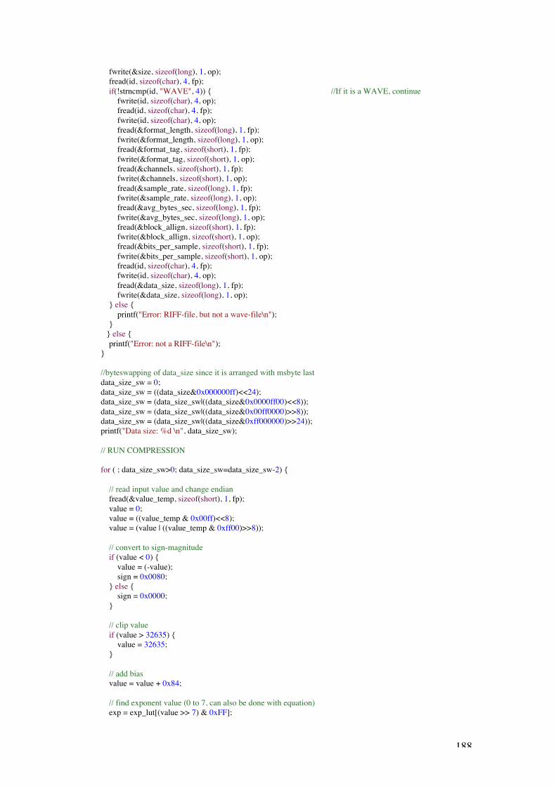
188

fwrite(&size, sizeof(long), 1, op); fread(id, sizeof(char), 4, fp); if(!strncmp(id, "WAVE", 4)) //If it is a WAVE, continue fwrite(id, sizeof(char), 4, op); fread(id, sizeof(char), 4, fp); fwrite(id, sizeof(char), 4, op); fread(&format_length, sizeof(long), 1, fp); fwrite(&format_length, sizeof(long), 1, op); fread(&format_tag, sizeof(short), 1, fp); fwrite(&format_tag, sizeof(short), 1, op); fread(&channels, sizeof(short), 1, fp); fwrite(&channels, sizeof(short), 1, op); fread(&sample_rate, sizeof(long), 1, fp); fwrite(&sample_rate, sizeof(long), 1, op); fread(&avg_bytes_sec, sizeof(long), 1, fp); fwrite(&avg_bytes_sec, sizeof(long), 1, op); fread(&block_allign, sizeof(short), 1, fp); fwrite(&block_allign, sizeof(short), 1, op); fread(&bits_per_sample, sizeof(short), 1, fp); fwrite(&bits_per_sample, sizeof(short), 1, op); fread(id, sizeof(char), 4, fp); fwrite(id, sizeof(char), 4, op); fread(&data_size, sizeof(long), 1, fp); fwrite(&data_size, sizeof(long), 1, op); else printf("Error: RIFF-file, but not a wave-file\n");

else printf("Error: not a RIFF-file\n");

//byteswapping of data_size since it is arranged with msbyte last data_size_sw = 0; data_size_sw = ((data_size&0x000000ff)<<24); data_size_sw = (data_size_sw|((data_size&0x0000ff00)<<8)); data_size_sw = (data_size_sw|((data_size&0x00ff0000)>>8)); data_size_sw = (data_size_sw|((data_size&0xff000000)>>24)); printf("Data size: %d \n", data_size_sw);

// RUN COMPRESSION

for ( ; data_size_sw>0; data_size_sw=data_size_sw-2)

// read input value and change endian fread(&value_temp, sizeof(short), 1, fp); value = 0; value = ((value_temp & 0x00ff)<<8); value = (value | ((value_temp & 0xff00)>>8));

// convert to sign-magnitude if (value < 0) value = (-value); sign = 0x0080; else sign = 0x0000;

// clip value if (value > 32635) value = 32635;

// add bias value = value + 0x84;

// find exponent value (0 to 7, can also be done with equation) exp = exp_lut[(value >> 7) & 0xFF];

189

// get the mantissa mantis = (value >> (exp + 3)) & 0x000f;

// put together output byte outputbuffer = (sign | (exp << 4) | mantis); fwrite(&outputbuffer, sizeof(char), 1, op); fclose(fp); fclose(op);

////////////////////////////////////////////////////////////////////////////////mu-law decoder, 2:1 compression...........………....////Works with 16-bit mono WAV-file on big-endian////systems..............................…………………….......////................................……………………….............////Ivar Løkken, Mar. 2004..............…………….......//////////////////////////////////////////////////////////////////////////////

#include <stdio.h>

// exponent recovery tablestatic int exp_lut[8] = 0,132,396,924,1980,4092,8316,16764;

int main(void) FILE *fp, *op;

fp = fopen("in.mul", "rb"); //open wav-file for reading op = fopen("out.wav", "wb"); //open output-file for writing

if (fp) //wav file info variables char id[4]; unsigned long size, data_size, data_size_sw; short format_tag, channels, block_allign, bits_per_sample; long format_length, sample_rate, avg_bytes_sec;

//data variables short valout = 0; //ouput value for writing unsigned char inputbuffer = 0; //input buffer char sign = 0; //sign char mantis = 0; //mantissa char exp = 0; //exponent short out = 0; //ouput variable

//read and write wav header info fread(id, sizeof(char), 4, fp); if(!strncmp(id, "RIFF", 4)) //if it is a RIFF, continue fwrite(id, sizeof(char), 4, op); fread(&size, sizeof(long), 1, fp); fwrite(&size, sizeof(long), 1, op); fread(id, sizeof(char), 4, fp); if(!strncmp(id, "WAVE", 4)) //if it is a WAVE, continue fwrite(id, sizeof(char), 4, op); fread(id, sizeof(char), 4, fp); fwrite(id, sizeof(char), 4, op); fread(&format_length, sizeof(long), 1, fp); fwrite(&format_length, sizeof(long), 1, op); fread(&format_tag, sizeof(short), 1, fp); fwrite(&format_tag, sizeof(short), 1, op); fread(&channels, sizeof(short), 1, fp); fwrite(&channels, sizeof(short), 1, op); fread(&sample_rate, sizeof(long), 1, fp);

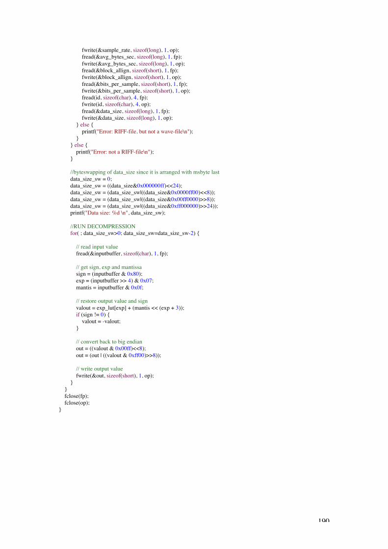
190

fwrite(&sample_rate, sizeof(long), 1, op); fread(&avg_bytes_sec, sizeof(long), 1, fp); fwrite(&avg_bytes_sec, sizeof(long), 1, op); fread(&block_allign, sizeof(short), 1, fp); fwrite(&block_allign, sizeof(short), 1, op); fread(&bits_per_sample, sizeof(short), 1, fp); fwrite(&bits_per_sample, sizeof(short), 1, op); fread(id, sizeof(char), 4, fp); fwrite(id, sizeof(char), 4, op); fread(&data_size, sizeof(long), 1, fp); fwrite(&data_size, sizeof(long), 1, op); else printf("Error: RIFF-file, but not a wave-file\n"); else printf("Error: not a RIFF-file\n");

//byteswapping of data_size since it is arranged with msbyte last data_size_sw = 0; data_size_sw = ((data_size&0x000000ff)<<24); data_size_sw = (data_size_sw|((data_size&0x0000ff00)<<8)); data_size_sw = (data_size_sw|((data_size&0x00ff0000)>>8)); data_size_sw = (data_size_sw|((data_size&0xff000000)>>24)); printf("Data size: %d \n", data_size_sw);

//RUN DECOMPRESSION for( ; data_size_sw>0; data_size_sw=data_size_sw-2)

// read input value fread(&inputbuffer, sizeof(char), 1, fp);

// get sign, exp and mantissa sign = (inputbuffer & 0x80); exp = (inputbuffer >> 4) & 0x07; mantis = inputbuffer & 0x0f;

// restore output value and sign valout = exp_lut[exp] + (mantis << (exp + 3)); if (sign != 0) valout = -valout;

// convert back to big endian out = ((valout & 0x00ff)<<8); out = (out | ((valout & 0xff00)>>8));

// write output value fwrite(&out, sizeof(short), 1, op); fclose(fp); fclose(op);

191

iLaw encoder and decoder:////////////////////////////////////////////////////////////////////////////////Custom mu-law-based encoder..........……….........////Works with 16-bit mono WAV-file on big-endian////systems...................................……………………..////.......................................………………………......////Ivar Løkken, Mar. 2004.............……………........//////////////////////////////////////////////////////////////////////////////

#include <stdio.h>

// mu-law exponential lookup tablestatic char exp_lut[256] = 0,0,1,1,2,2,2,2,3,3,3,3,3,3,3,3, 4,4,4,4,4,4,4,4,4,4,4,4,4,4,4,4, 5,5,5,5,5,5,5,5,5,5,5,5,5,5,5,5, 5,5,5,5,5,5,5,5,5,5,5,5,5,5,5,5, 6,6,6,6,6,6,6,6,6,6,6,6,6,6,6,6, 6,6,6,6,6,6,6,6,6,6,6,6,6,6,6,6, 6,6,6,6,6,6,6,6,6,6,6,6,6,6,6,6, 6,6,6,6,6,6,6,6,6,6,6,6,6,6,6,6, 7,7,7,7,7,7,7,7,7,7,7,7,7,7,7,7, 7,7,7,7,7,7,7,7,7,7,7,7,7,7,7,7, 7,7,7,7,7,7,7,7,7,7,7,7,7,7,7,7, 7,7,7,7,7,7,7,7,7,7,7,7,7,7,7,7, 7,7,7,7,7,7,7,7,7,7,7,7,7,7,7,7, 7,7,7,7,7,7,7,7,7,7,7,7,7,7,7,7, 7,7,7,7,7,7,7,7,7,7,7,7,7,7,7,7, 7,7,7,7,7,7,7,7,7,7,7,7,7,7,7,7;

static int exp_lut2[8] = 0,132,396,924,1980,4092,8316,16764;

int main(void) FILE *fp, *op;

fp = fopen("in.wav", "rb"); //open wav-file for reading op = fopen("out.mul", "wb"); //open output-file for writing

if (fp) //wav file info variables char id[4]; unsigned long size, data_size, data_size_sw, loop; short format_tag, channels, block_allign, bits_per_sample; long format_length, sample_rate, avg_bytes_sec;

//predictor variables short value = 0; //current input sample value short value_temp = 0; //temp value short valprev = 0; //previous value int dif; //first order prediction value int dif2 = 0; //second order prediction value short d2 = 0; //predictor output int difprev = 0; //previous first order prediction value int d2o; //decoded error value for feedback

//encoder variables unsigned short sign = 0; //sign-bit unsigned short exp = 0; //exponent (position of rightmost 1) unsigned short mantis = 0; //mantissa unsigned short outputbuffer[8]; //output buffer unsigned short shortbuffer[5]; //16-bit buffer for writing to file as short int i = 0;

192

//read and write wav info fread(id, sizeof(char), 4, fp); if(!strncmp(id, "RIFF", 4)) //if it is a RIFF, continue fwrite(id, sizeof(char), 4, op);

fread(&size, sizeof(long), 1, fp); fwrite(&size, sizeof(long), 1, op); fread(id, sizeof(char), 4, fp); if(!strncmp(id, "WAVE", 4)) //If it is a WAVE, continue fwrite(id, sizeof(char), 4, op); fread(id, sizeof(char), 4, fp); fwrite(id, sizeof(char), 4, op); fread(&format_length, sizeof(long), 1, fp); fwrite(&format_length, sizeof(long), 1, op); fread(&format_tag, sizeof(short), 1, fp); fwrite(&format_tag, sizeof(short), 1, op); fread(&channels, sizeof(short), 1, fp); fwrite(&channels, sizeof(short), 1, op); fread(&sample_rate, sizeof(long), 1, fp); fwrite(&sample_rate, sizeof(long), 1, op); fread(&avg_bytes_sec, sizeof(long), 1, fp); fwrite(&avg_bytes_sec, sizeof(long), 1, op); fread(&block_allign, sizeof(short), 1, fp); fwrite(&block_allign, sizeof(short), 1, op); fread(&bits_per_sample, sizeof(short), 1, fp); fwrite(&bits_per_sample, sizeof(short), 1, op); fread(id, sizeof(char), 4, fp); fwrite(id, sizeof(char), 4, op); fread(&data_size, sizeof(long), 1, fp); fwrite(&data_size, sizeof(long), 1, op); else printf("Error: RIFF-file, but not a wave-file\n");

else printf("Error: not a RIFF-file\n");

//byteswapping of data_size since it is arranged with msbyte last data_size_sw = 0; data_size_sw = ((data_size&0x000000ff)<<24); data_size_sw = (data_size_sw|((data_size&0x0000ff00)<<8)); data_size_sw = (data_size_sw|((data_size&0x00ff0000)>>8)); data_size_sw = (data_size_sw|((data_size&0xff000000)>>24)); loop = data_size_sw/16; printf("Data size: %d \n", data_size_sw);

// RUN COMPRESSION

for ( ; loop>0; loop=loop-1)

for(i=0; i<=7;i++)

// read input value and change endian fread(&value_temp, sizeof(short), 1, fp); value = 0; value = ((value_temp & 0x00ff)<<8); value = (value | ((value_temp & 0xff00)>>8));

// second order linear prediction dif = value - valprev; dif2 = dif - difprev;

//toss away LSB since the mulaw will do that anyway d2 = dif2>>1;

// convert to sign-magnitude if (d2 < 0) d2 = (-d2);

193

sign = 0x0200; else sign = 0x0000;

// clip value if (d2 > 32635) d2 = 32635;

// add bias d2 = d2 + 0x84;

// find exponent value (0 to 7) exp = exp_lut[(d2 >> 7) & 0xFF];

// get the mantissa mantis = (d2 >> (exp + 1)) & 0x003f;

// put together output byte outputbuffer[i] = (sign | (exp << 6) | mantis) & 0x03ff;

// decode error value d2o = (exp_lut2[exp] + (mantis << (exp + 1)))<<1; if (sign != 0) d2o = -d2o; difprev += d2o; valprev += difprev;

//put together output variable //outputbuffer holds 10 compressed samples or 80 bytes

shortbuffer[0]=outputbuffer[0]|outputbuffer[1]<<10; shortbuffer[1]=(outputbuffer[1]>>6)|(outputbuffer[2]<<4)|(outputbuffer[3]<<14); shortbuffer[2]=(outputbuffer[3]>>2)|(outputbuffer[4]<<8); shortbuffer[3]=(outputbuffer[4]>>8)|(outputbuffer[5]<<2)|(outputbuffer[6]<<12); shortbuffer[4]=(outputbuffer[6]>>4)|outputbuffer[7]<<6;

// write output value for(i=0; i <= 4; i++) fwrite(&shortbuffer[i], sizeof(short), 1, op); fclose(fp); fclose(op);

////////////////////////////////////////////////////////////////////////////////Custom mu-law-based decoder.............………......////Works with 16-bit mono WAV-file on big-endian////systems.............................……………………........////..................................………………………...........////Ivar Løkken, Mar. 2004.........……………............//////////////////////////////////////////////////////////////////////////////

#include <stdio.h>

//exponent recovery table

194

static int exp_lut[8] = 0,132,396,924,1980,4092,8316,16764;//static int exp_lut[8] = 0,

int main(void) FILE *fp, *op;

fp = fopen("in.mul", "rb"); //open wav-file for reading op = fopen("out.wav", "wb"); //open output-file for writing

if (fp)

//wav info variables char id[4]; unsigned long size, data_size, data_size_sw, loop; short format_tag, channels, block_allign, bits_per_sample; long format_length, sample_rate, avg_bytes_sec;

//data variables unsigned short inputbuffer[5]; //input buffer unsigned short tempbuffer[8]; //decoded sample buffer int valout = 0; //ouput value for writing char i; //counting variable

//decoder variables unsigned short sign = 0; unsigned short mantis = 0; unsigned short exp = 0;

//predictor short out = 0; //output variable int difout = 0; //difference int d1out = 0; //difference of differences (2nd order)

//read and write wav info fread(id, sizeof(char), 4, fp); if(!strncmp(id, "RIFF", 4)) //if it is a RIFF, continue fwrite(id, sizeof(char), 4, op); fread(&size, sizeof(long), 1, fp); fwrite(&size, sizeof(long), 1, op); fread(id, sizeof(char), 4, fp); if(!strncmp(id, "WAVE", 4)) //if it is a WAVE, continue fwrite(id, sizeof(char), 4, op); fread(id, sizeof(char), 4, fp); fwrite(id, sizeof(char), 4, op); fread(&format_length, sizeof(long), 1, fp); fwrite(&format_length, sizeof(long), 1, op); fread(&format_tag, sizeof(short), 1, fp); fwrite(&format_tag, sizeof(short), 1, op); fread(&channels, sizeof(short), 1, fp); fwrite(&channels, sizeof(short), 1, op); fread(&sample_rate, sizeof(long), 1, fp); fwrite(&sample_rate, sizeof(long), 1, op); fread(&avg_bytes_sec, sizeof(long), 1, fp); fwrite(&avg_bytes_sec, sizeof(long), 1, op); fread(&block_allign, sizeof(short), 1, fp); fwrite(&block_allign, sizeof(short), 1, op); fread(&bits_per_sample, sizeof(short), 1, fp); fwrite(&bits_per_sample, sizeof(short), 1, op); fread(id, sizeof(char), 4, fp); fwrite(id, sizeof(char), 4, op); fread(&data_size, sizeof(long), 1, fp); fwrite(&data_size, sizeof(long), 1, op); else printf("Error: RIFF-file, but not a wave-file\n"); else

195

printf("Error: not a RIFF-file\n");

//byteswapping of data_size since it is arranged withmsbyte last data_size_sw = 0; data_size_sw = ((data_size&0x000000ff)<<24); data_size_sw = (data_size_sw|((data_size&0x0000ff00)<<8)); data_size_sw = (data_size_sw|((data_size&0x00ff0000)>>8)); data_size_sw = (data_size_sw|((data_size&0xff000000)>>24)); printf("Data size: %d \n", data_size_sw); loop = data_size_sw/16;

//RUN DECOMPRESSION for( ; loop>0; loop=loop-1)

// read input values for(i=0; i <= 4; i++) fread(&inputbuffer[i], sizeof(short), 1, fp);

//put samples in to separate buffer places tempbuffer[0]= inputbuffer[0] & 0x03ff; tempbuffer[1]= 0x03ff & ((0x003f&(inputbuffer[0]>>10))|(0x03c0&(inputbuffer[1]<<6))); tempbuffer[2]= 0x03ff & (inputbuffer[1]>>4); tempbuffer[3]= 0x03ff & ((0x0003&(inputbuffer[1]>>14))|(0x03fc&(inputbuffer[2]<<2))); tempbuffer[4]= 0x03ff & ((0x00ff&(inputbuffer[2]>>8))|(0x0300&(inputbuffer[3]<<8))); tempbuffer[5]= 0x03ff & (inputbuffer[3]>>2); tempbuffer[6]= 0x03ff & ((0x000f&(inputbuffer[3]>>12))|(0x03f0&(inputbuffer[4]<<4))); tempbuffer[7]= 0x03ff & (inputbuffer[4]>>6);

//RUN DECOMPRESSION for(i=0; i<= 7; i++)

//find sign, exponent, mantissa sign = tempbuffer[i] & 0x0200; exp = (tempbuffer[i]>>6) & 0x0007; mantis = (tempbuffer[i] & 0x003f);

// restore output value difout = (exp_lut[exp] + (mantis << (exp+1)))<<1; if (sign != 0) difout = -difout;

//prediction d1out += difout; valout += d1out;

//clip output value if (valout>32767) valout = 32767; if (valout<-32768) valout = -32768;

// convert back to big endian out = ((valout & 0x00ff)<<8); out = (out | ((valout & 0xff00)>>8));

// write output value fwrite(&out, sizeof(short), 1, op); fclose(fp); fclose(op);

196

Entropy coding tester, Rice-, Pod- and iPod encoder anddecoder/////////////////////////////////////////////////////////////////////entropy coding test program................……////pod vs rice vs ipod test encoder...........…...////no prediction, but it......................………...////can easily be included in main if desired...////...........................................………………..////Ivar Løkken, NTNU 2004.....................….////x86 users, remove byteswapping.............…////////////////////////////////////////////////////////////////////

#include <stdio.h>

// table for output bitshiftstatic unsigned short bittab[16] = 0x0001,0x0002,0x0004,0x0008,0x0010,0x0020,0x0040,0x0080, 0x0100,0x0200,0x0400,0x0800,0x1000,0x2000,0x4000,0x8000;

FILE *fp, *op, *tp;

//wav file info variableschar id[4];unsigned long size, data_size, data_size_sw;short format_tag, channels, block_allign, bits_per_sample;long format_length, sample_rate, avg_bytes_sec;

//data variablesshort value = 0; //current input sample valueshort value_temp = 0; //temp valueunsigned short out = 0; //output variableunsigned short maxwordlength = 0; //max wordlength indicatorunsigned char coding = 0; //Pod or Rice selectorunsigned char prefixbits = 0; //number of bits in the prefix

//encoder variablesunsigned short sign = 0; //sign-bitunsigned short overflow = 0; //binary partunsigned char numzeros = 0; //number of zerosunsigned char k = 6;unsigned long A = 0; //accumulated value for calculation of kunsigned char N = 0; //sample countshort i = 0; //counting variableshort j = 15; //counting variableshort x = 0; //how often is new k calculated

//encoder functionsvoid pod_encoder(void);void rice_encoder(void);void ipod_encoder(void);

int main(void)

fp = fopen("in.wav", "rb"); //open wav-file for reading op = fopen("out.comp", "wb"); //open output-file for writing tp = fopen("test.hex", "wb"); //test file for whatever the user wants to store

if (fp) //read and write wav header fread(id, sizeof(char), 4, fp); if(!strncmp(id, "RIFF", 4)) //if it is a RIFF, continue

197

fwrite(id, sizeof(char), 4, op); fread(&size, sizeof(long), 1, fp); fwrite(&size, sizeof(long), 1, op); fread(id, sizeof(char), 4, fp); if(!strncmp(id, "WAVE", 4)) //If it is a WAVE, continue fwrite(id, sizeof(char), 4, op); fread(id, sizeof(char), 4, fp); fwrite(id, sizeof(char), 4, op); fread(&format_length, sizeof(long), 1, fp); fwrite(&format_length, sizeof(long), 1, op); fread(&format_tag, sizeof(short), 1, fp); fwrite(&format_tag, sizeof(short), 1, op); fread(&channels, sizeof(short), 1, fp); fwrite(&channels, sizeof(short), 1, op); fread(&sample_rate, sizeof(long), 1, fp); fwrite(&sample_rate, sizeof(long), 1, op); fread(&avg_bytes_sec, sizeof(long), 1, fp); fwrite(&avg_bytes_sec, sizeof(long), 1, op); fread(&block_allign, sizeof(short), 1, fp); fwrite(&block_allign, sizeof(short), 1, op); fread(&bits_per_sample, sizeof(short), 1, fp); fwrite(&bits_per_sample, sizeof(short), 1, op); fread(id, sizeof(char), 4, fp); fwrite(id, sizeof(char), 4, op); fread(&data_size, sizeof(long), 1, fp); fwrite(&data_size, sizeof(long), 1, op); else printf("Error: RIFF-file, but not a wave-file\n");

else printf("Error: not a RIFF-file\n");

//byteswapping of data_size since it is arranged with msbyte last data_size_sw = 0; data_size_sw = ((data_size&0x000000ff)<<24); data_size_sw = (data_size_sw|((data_size&0x0000ff00)<<8)); data_size_sw = (data_size_sw|((data_size&0x00ff0000)>>8)); data_size_sw = (data_size_sw|((data_size&0xff000000)>>24)); printf("Data size: %d \n", data_size_sw);

// RUN COMPRESSION printf("Please select encoding method (0 = Pod-coding, 1 = Rice-coding, 2 = iPod-coding): "); scanf("%u", &coding); if (coding == 0) pod_encoder(); else if (coding == 1)

rice_encoder; else if (coding == 2)

ipod_encoder(); fclose(op); fclose(fp); fclose(tp);

//pod encodervoid pod_coder(void) for ( ; data_size_sw>0; data_size_sw=data_size_sw-2)

// read input value and change endian fread(&value_temp, sizeof(short), 1, fp); value = 0; value = ((value_temp & 0x00ff)<<8);

198

value = (value | ((value_temp & 0xff00)>>8));

// convert to sign-magnitude if (value < 0) value = (-value); sign = 1; else sign = 0;

// perform Pod-coding

// find overflow overflow = 0; overflow = value >> k; fwrite(&numzeros, sizeof(char), 1, tp);

// find number of zeros numzeros = 0; // overflow can be max (16-k) bits for (i=0;i<(16-k);i++) if (overflow > (bittab[i]-1)) numzeros++; else

break;

// find max wordlength just to see how the coding performs if (((numzeros<<1)+k+1) > maxwordlength) maxwordlength = (numzeros<<1)+k+2;

// put together and write output data bit by bit // data fills the out-variable continuously from // MSB and downwards // using bit-table, bittable[j] is a 1 in position // j counting from LSB to MSB // when out-variable is filled (j<0), it starts // filling out a new one immideately

// sign if (sign != 0) out = out | bittab[j]; j--; if (j<0) fwrite(&out, sizeof(short), 1, op); j=15; out = 0;

// zeros followed by overflow or just a one if the overflow is 0 if (numzeros == 0) out = out | bittab[j]; j--; if (j<0)

fwrite(&out, sizeof(short), 1, op); j=15; out=0;

else //zeros for (i=numzeros; i>0; i--)

j--; if (j<0) fwrite(&out, sizeof(short), 1, op);

199

j=15; out=0;

// overflow for (i=numzeros; i>0; i--) if ((overflow & bittab[i-1]) != 0) out = out | bittab[j]; j--; if (j<0)

fwrite(&out, sizeof(short), 1, op); j=15; out = 0;

// uncoded part (bit 1 to bit k of value) for (i=k; i>0; i--) if ((value & bittab[i-1]) != 0)

out = out | bittab[j]; j--; if (j<0) fwrite(&out, sizeof(short), 1, op);

j = 15; out = 0;

// calculate k for next sample N++; A+=value; x++; // if x=n in IF, k is calculated every n samples. Remove if to // calculate k for every sample //if (x==64 || N == 255) for (k=0; (N<<k)<A; k++); x = 0; // // reset accumulation every 255th sample if (N==255) N=0; A=0; printf("Max wordlength: %d \n", maxwordlength);

//rice encodervoid rice_encoder(void) for ( ; data_size_sw>0; data_size_sw=data_size_sw-2)

// read input value and change endian fread(&value_temp, sizeof(short), 1, fp); value = 0; value = ((value_temp & 0x00ff)<<8); value = (value | ((value_temp & 0xff00)>>8));

// convert to sign-magnitude if (value < 0) value = (-value); sign = 1; else

200

sign = 0; // perform Rice-coding

// find overflow overflow = 0; overflow = value >> k;

// find max wordlength just to see how the coding performs // in worst-case if ((overflow+k+2) > maxwordlength)

maxwordlength = overflow + k + 2; // put together and write output data bit by bit // data fills the out-variable continuously from // MSB and downwards // using bit-table, bittable[j] is a 1 in position // j counting from LSB to MSB // when out-variable is filled (j<0), it starts // filling out a new one immideately

// sign if (sign != 0)

out = out | bittab[j]; j--; if (j<0)

fwrite(&out, sizeof(short), 1, op); j=15; out = 0;

// (overflow) zeros followed by terminating 1 for (i=overflow ; i>0; i--)

j--; if (j<0) fwrite(&out, sizeof(short), 1, op); j=15; out=0;

out = out | bittab[j]; j--; if (j<0)

fwrite(&out, sizeof(short), 1, op); j=15; out=0;

// uncoded part (bit 1 to bit k of value) for (i=k; i>0; i--) if ((value & bittab[i-1]) != 0)

out = out | bittab[j]; j--; if (j<0) fwrite(&out, sizeof(short), 1, op); j = 15; out = 0;

// calculate k for next sample N++; A+=value; x++;

201

//new k is calculated for every n samples, where (x==n) is given in if //comment out if when you want new k calculated for every sample //if (x==4 || N ==255) for (k=0; (N<<k)<A; k++);

x=0; // // reset accumulation every 255th sample if (N==255)

N=0; A=0;

printf("Max wordlength: %d \n", maxwordlength);

//iPod encodervoid ipod_encoder(void) for ( ; data_size_sw>0; data_size_sw=data_size_sw-2)

// read input value and change endian fread(&value_temp, sizeof(short), 1, fp); value = 0; value = ((value_temp & 0x00ff)<<8); value = (value | ((value_temp & 0xff00)>>8));

// convert to sign-magnitude if (value < 0)

value = (-value); sign = 1;

else sign = 0;

// perform iPod-coding

// find overflow overflow = 0; overflow = value >> k; // shift coding up one number overflow = overflow + 1; fwrite(&prefixbits, sizeof(char), 1, tp);

// find number of bits in prefix prefixbits = 0; // overflow can be max (16-k) bits for (i=0;i<(16-k);i++)

if (overflow > (bittab[i]-1)) prefixbits++; else break;

// find max wordlength just to see how the coding performs if (((prefixbits<<1)+k+1) > maxwordlength)

maxwordlength = (prefixbits<<1)+k+2;

// put together and write output data bit by bit // data fills the out-variable continuously from // MSB and downwards // using bit-table, bittable[j] is a 1 in position // j counting from LSB to MSB // when out-variable is filled (j<0), it starts // filling out a new one immideately

202

// if the value is positive if (sign == 0)

// zeros followed by overflow

//zeros for (i=prefixbits; i>0; i--) j--; if (j<0)

fwrite(&out, sizeof(short), 1, op);j=15;out=0;

// overflow for (i=prefixbits; i>0; i--) if ((overflow & bittab[i-1]) != 0)

out = out | bittab[j]; j--; if (j<0)

fwrite(&out, sizeof(short), 1, op);j=15;out = 0;

// if the value is negative, output 1's and inverted overflow else if (sign == 1) //ones

for (i=prefixbits; i>0; i--) out = out | bittab[j]; j--; if (j<0)

fwrite(&out, sizeof(short), 1, op);j=15;out=0;

// inverted overflow for (i=prefixbits; i>0; i--) if ((overflow & bittab[i-1]) == 0)

out = out | bittab[j]; j--; if (j<0)

fwrite(&out, sizeof(short), 1, op);j=15;out = 0;

// uncoded part (bit 1 to bit k of value) for (i=k; i>0; i--)

if ((value & bittab[i-1]) != 0) out = out | bittab[j]; j--; if (j<0) fwrite(&out, sizeof(short), 1, op); j = 15; out = 0;

// calculate k for next sample

203

N++; A+=value; x++; // if x=n in IF, k is calculated every n samples. Remove if to // calculate k for every sample //if (x==64 || N == 255) for (k=0; (N<<k)<A; k++);

x = 0; // // reset accumulation every 255th sample if (N==255)

N=0; A=0;

printf("Max wordlength: %d \n", maxwordlength);

/////////////////////////////////////////////////////////////////////entropy coding test program................……////pod vs rice vs ipod test decoder...........…...////no prediction, but it......................………...////can easily be included in main if desired...////...........................................………………..////Ivar Løkken, NTNU 2004.....................….////x86 users, remove byteswapping.............…////////////////////////////////////////////////////////////////////

#include <stdio.h>

// table for output bitshiftstatic unsigned short bittab[16] = 0x0001,0x0002,0x0004,0x0008,0x0010,0x0020,0x0040,0x0080, 0x0100,0x0200,0x0400,0x0800,0x1000,0x2000,0x4000,0x8000;

FILE *fp, *op, *tp;

//wav file info variableschar id[4];unsigned long size, data_size, data_size_sw;short format_tag, channels, block_allign, bits_per_sample;long format_length, sample_rate, avg_bytes_sec;

//data variablesunsigned short in = 0; //input variable variableshort out = 0;short valout = 0;unsigned short maxwordlength = 0; //max wordlength indicatorunsigned char coding = 0; //Pod or Rice selectorunsigned char prefixbits = 0; //number of bits in the prefix

//decoder variablesunsigned short sign = 0; //sign-bitunsigned short overflow = 0; //binary partunsigned char numzeros = 0; //number of zerosunsigned char k = 6;unsigned long A = 0; //accumulated value for calculation of kunsigned char N = 0; //sample countshort i = 0; //counting variableshort j = 15; //counting variableshort x = 0; //how often is new k calculated

//decoder functionsvoid pod_decoder(void);void rice_decoder(void);void ipod_decoder(void);

204

int main(void)

fp = fopen("out.comp", "rb"); //open wav-file for reading op = fopen("out.wav", "wb"); //open output-file for writing tp = fopen("testd.hex", "wb"); //test file for whatever the user wants to store

if (fp) //read and write wav header fread(id, sizeof(char), 4, fp); if(!strncmp(id, "RIFF", 4)) //if it is a RIFF, continue fwrite(id, sizeof(char), 4, op); fread(&size, sizeof(long), 1, fp); fwrite(&size, sizeof(long), 1, op); fread(id, sizeof(char), 4, fp); if(!strncmp(id, "WAVE", 4)) //If it is a WAVE, continue fwrite(id, sizeof(char), 4, op); fread(id, sizeof(char), 4, fp); fwrite(id, sizeof(char), 4, op); fread(&format_length, sizeof(long), 1, fp); fwrite(&format_length, sizeof(long), 1, op); fread(&format_tag, sizeof(short), 1, fp); fwrite(&format_tag, sizeof(short), 1, op); fread(&channels, sizeof(short), 1, fp); fwrite(&channels, sizeof(short), 1, op); fread(&sample_rate, sizeof(long), 1, fp); fwrite(&sample_rate, sizeof(long), 1, op); fread(&avg_bytes_sec, sizeof(long), 1, fp); fwrite(&avg_bytes_sec, sizeof(long), 1, op); fread(&block_allign, sizeof(short), 1, fp); fwrite(&block_allign, sizeof(short), 1, op); fread(&bits_per_sample, sizeof(short), 1, fp); fwrite(&bits_per_sample, sizeof(short), 1, op); fread(id, sizeof(char), 4, fp); fwrite(id, sizeof(char), 4, op); fread(&data_size, sizeof(long), 1, fp); fwrite(&data_size, sizeof(long), 1, op); else printf("Error: RIFF-file, but not a wave-file\n");

else printf("Error: not a RIFF-file\n");

//byteswapping of data_size since it is arranged with msbyte last data_size_sw = 0; data_size_sw = ((data_size&0x000000ff)<<24); data_size_sw = (data_size_sw|((data_size&0x0000ff00)<<8)); data_size_sw = (data_size_sw|((data_size&0x00ff0000)>>8)); data_size_sw = (data_size_sw|((data_size&0xff000000)>>24)); printf("Data size: %d \n", data_size_sw);

// RUN COMPRESSION printf("Please select decoding method (0 = Pod-coding, 1 = Rice-coding, 2 = iPod-coding): "); scanf("%u", &coding); if (coding == 0)

pod_decoder(); else if (coding == 1)

rice_decoder; else if (coding == 2)

ipod_decoder(); fclose(op);

205

fclose(fp); fclose(tp);

//Pod decoder functionvoid pod_decoder(void) //read the 16 first bits fread(&in, sizeof(short), 1, fp);

for ( ; data_size_sw>0; data_size_sw=data_size_sw-2)

// read sign sign = in & bittab[j]; j--;

if (j<0) fread(&in, sizeof(short), 1, fp); j = 15;

// count zeros numzeros = 0; while ((in & bittab[j]) == 0)

numzeros++; j--;

if (j<0) fread(&in, sizeof(short), 1, fp);

j = 15; fwrite(&numzeros, sizeof(char), 1, tp);

// if numzeros = 0, skip the "1" prefix if (numzeros == 0)

j--; if (j<0) fread(&in, sizeof(short), 1, fp); j = 15;

// read the next part (numzeros and k bits) bit by bit and construct output valout = 0; for (i=(numzeros+k) ; i>0; i--)

if ((in & bittab[j]) != 0) valout = valout | bittab[i-1]; j--; if (j<0) fread(&in, sizeof(short), 1, fp); j = 15;

// calculate k for next sample // if x=n in IF, k is calculated every n samples. Remove if to // calculate k for every sample N++; A += valout; x++; //if (x==3 || N == 255)

for (k=0; (N<<k)<A; k++); x = 0;

//

// reset accumulation every 255th sample if (N==255)

N=0;

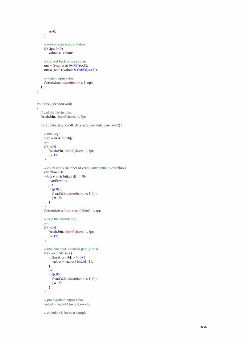
206

A=0;

// restore sign representation if (sign != 0)

valout = -valout;

// convert back to big endian out = ((valout & 0x00ff)<<8); out = (out | ((valout & 0xff00)>>8));

// write output value fwrite(&out, sizeof(short), 1, op);

void rice_decoder(void) //read the 16 first bits fread(&in, sizeof(short), 1, fp);

for ( ; data_size_sw>0; data_size_sw=data_size_sw-2)

// read sign sign = in & bittab[j]; j--; if (j<0)

fread(&in, sizeof(short), 1, fp); j = 15;

// count zeros (number of zeros correspond to overflow) overflow = 0; while ((in & bittab[j]) == 0)

overflow++; j--; if (j<0) fread(&in, sizeof(short), 1, fp); j = 15;

fwrite(&overflow, sizeof(short), 1, tp);

// skip the terminating 1 j--; if (j<0)

fread(&in, sizeof(short), 1, fp); j = 15;

// read the next, uncoded part (k bits) for (i=k ; i>0; i--)

if ((in & bittab[j]) != 0) valout = valout | bittab[i-1]; j--; if (j<0) fread(&in, sizeof(short), 1, fp); j = 15;

// put together output value valout = valout | (overflow<<k);

// calculate k for next sample

207

N++; A += valout; x++; //new k is calculated for every n+1 samples, where (x==n) is given in if //comment out if when you want new k calculated for every sample //if (x==4 || N==65535) for (k=0; (N<<k)<A; k++);

x = 0; // // reset accumulation every 255th sample if (N==255)

N=0; A=0;

// restore sign representation if (sign != 0)

valout = -valout;

// convert back to big endian out = ((valout & 0x00ff)<<8); out = (out | ((valout & 0xff00)>>8));

// write output value fwrite(&out, sizeof(short), 1, op); valout = 0; out = 0;

void ipod_decoder(void) //read the 16 first bits fread(&in, sizeof(short), 1, fp);

for ( ; data_size_sw>0; data_size_sw=data_size_sw-2)

// read first bit to see if value is positive or negative if (in & bittab[j] == 0)

sign = 0; // if first bit zero, non inverted prefix, count zeros prefixbits = 0; while ((in & bittab[j]) == 0) prefixbits++; j--; if (j<0)

fread(&in, sizeof(short), 1, fp);j = 15;

// and put overflow to variable for (i=(prefixbits); i>0; i--) if (in & bittab[j] != 0)

overflow = overflow | bittab[i-1]; j--; if (j<0)

fread(&in, sizeof(short), 1, fp);j = 15;

else // if first bit is one, inverted prefix, count ones sign = 1; prefixbits = 0; while ((in & bittab[j]) != 0)

fwrite((in&bittab[j]), sizeof(short), 1, tp);

208

prefixbits++; j--;

if (j<0) fread(&in, sizeof(short), 1, fp); j = 15;

fclose(tp); // and put "deinverted" overflow to variable for (i=(prefixbits); i>0; i--) if (in & bittab[j] == 0)

overflow = overflow | bittab[i-1];

j--; if (j<0) fread(&in, sizeof(short), 1, fp); j = 15;

// remove upshift overflow = overflow - 1; valout = 0; valout = (overflow << k);

// read the next part (k bits) bit by bit and construct output for (i=k ; i>0; i--)

if ((in & bittab[j]) != 0) valout = valout | bittab[i-1]; j--; if (j<0) fread(&in, sizeof(short), 1, fp); j = 15;

// calculate k for next sample // if x=n in IF, k is calculated every n samples. Remove if to // calculate k for every sample N++; A += valout; x++; //if (x==3 || N == 255) for (k=0; (N<<k)<A; k++);

x = 0; //

// reset accumulation every 255th sample if (N==255)

N=0; A=0;

// restore sign representation if (sign != 0)

valout = -valout;

// convert back to big endian out = ((valout & 0x00ff)<<8); out = (out | ((valout & 0xff00)>>8));

// write output value fwrite(&out, sizeof(short), 1, op);

209

Final lossless codec, encoder and decoder////////////////////////////////////////////////////////////////////////compression test program..........……….........////pod-encoding........................……………......////selectable prediction......................……….…////from no prediction up to fourth order....…...////mono or stereo.............................…………...////...........................................………………….////Written for Macintosh, Intel users remove...////endian conversion....................………….......////........................................…………………....////encoder...............................……………........////.........................................…………………...////Ivar Løkken, NTNU, 2004............……........///////////////////////////////////////////////////////////////////////

#include <stdio.h>

// table for output bitshiftstatic unsigned long bittab[32] = 0x00000001,0x00000002,0x00000004,0x00000008,0x00000010,0x00000020,0x00000040,0x00000080, 0x00000100,0x00000200,0x00000400,0x00000800,0x00001000,0x00002000,0x00004000,0x00008000, 0x00010000,0x00020000,0x00040000,0x00080000,0x00100000,0x00200000,0x00400000,0x00800000, 0x01000000,0x02000000,0x04000000,0x08000000,0x10000000,0x20000000,0x40000000,0x80000000;

//predictor variableslong valprev[2] = 0,0; //previous valuelong diff[2] = 0,0; //differencelong diffprev[2] = 0,0; //previous differencelong diff2[2] = 0,0; //second order differencelong diff2prev[2] = 0,0; //previous second order differencelong diff3[2] = 0,0; //and so forth, [2] because of stereolong diff3prev[2] = 0,0; //one for each channellong diff4[2] = 0,0;long diff4prev[2] = 0,0;long residual = 0; //prediction residual

//encoder variablesunsigned short sign = 0; //sign-bitunsigned short overflow = 0; //binary partunsigned char numzeros = 0; //number of zerosunsigned char k[2] = 6,6; //k-variable, output wordlength estimationunsigned long A[2] = 0,0; //accumulated value for calculation of kunsigned char N[2] = 0,0; //sample countint chandec = 0; //channel decorrelation indicator

//data variablesshort value = 0; //current input sample valueshort value_temp = 0; //temp valueshort left = 0; //left channel valueshort right = 0; //right channel valuelong side = 0; //Side = L-R

//misc. variablesshort i = 0; //counting variableshort j = 15; //counting variableunsigned char m = 0; //left/right indicatorshort x = 0; //how often is new k calculatedunsigned short out = 0; //output variableunsigned short maxwordlength = 0; //max wordlength indicatorint order = 0; //prediction order

//compress function

210

void compress(long invalue);FILE *fp, *op, *tp;

//main routineint main(void) fp = fopen("reference.wav", "rb"); //open wav-file for reading op = fopen("out.comp", "wb"); //open output-file for writing tp = fopen("test.hex", "wb"); //test file for whatever test data

//the user will include if (fp) //wav header variables char id[4]; unsigned long size, data_size, data_size_sw; short format_tag, channels, channels_temp, block_allign, bits_per_sample; long format_length, sample_rate, avg_bytes_sec;

// read wave header and copy it to output file fread(id, sizeof(char), 4, fp); if(!strncmp(id, "RIFF", 4)) //if it is a RIFF, continue fwrite(id, sizeof(char), 4, op); fread(&size, sizeof(long), 1, fp); fwrite(&size, sizeof(long), 1, op); fread(id, sizeof(char), 4, fp); if(!strncmp(id, "WAVE", 4)) //If it is a WAVE, continue fwrite(id, sizeof(char), 4, op); fread(id, sizeof(char), 4, fp); fwrite(id, sizeof(char), 4, op); fread(&format_length, sizeof(long), 1, fp); fwrite(&format_length, sizeof(long), 1, op); fread(&format_tag, sizeof(short), 1, fp); fwrite(&format_tag, sizeof(short), 1, op); fread(&channels_temp, sizeof(short), 1, fp); fwrite(&channels_temp, sizeof(short), 1, op); fread(&sample_rate, sizeof(long), 1, fp); fwrite(&sample_rate, sizeof(long), 1, op); fread(&avg_bytes_sec, sizeof(long), 1, fp); fwrite(&avg_bytes_sec, sizeof(long), 1, op); fread(&block_allign, sizeof(short), 1, fp); fwrite(&block_allign, sizeof(short), 1, op); fread(&bits_per_sample, sizeof(short), 1, fp); fwrite(&bits_per_sample, sizeof(short), 1, op); fread(id, sizeof(char), 4, fp); fwrite(id, sizeof(char), 4, op); fread(&data_size, sizeof(long), 1, fp); fwrite(&data_size, sizeof(long), 1, op); else printf("Error: RIFF-file, but not a wave-file\n"); else printf("Error: not a RIFF-file\n");

//byteswapping of data_size since it is arranged with msbyte last data_size_sw = 0; data_size_sw = ((data_size&0x000000ff)<<24); data_size_sw = (data_size_sw|((data_size&0x0000ff00)<<8)); data_size_sw = (data_size_sw|((data_size&0x00ff0000)>>8)); data_size_sw = (data_size_sw|((data_size&0xff000000)>>24)); printf("Data size: %d \n", data_size_sw);

//select parameters printf("Select prediction order (0, 1, 2, 3 or 4): "); scanf("%u", &order); printf("%u", order); printf("\nDo you want to include channel decorrelation (0=no, 1=yes)? "); scanf("%u", &chandec);

211

printf("%u", chandec);

// RUN COMPRESSION

for ( ; data_size_sw>0; data_size_sw=data_size_sw-2)

// check if order is ok if (order < 0 | order > 4) printf("Error, invalid prediction order \n"); break; // byteswap channels variable channels = ((channels_temp & 0x00ff)<<8);

channels = (channels | ((channels_temp & 0xff00)>>8));

//if the file is mono if (channels == 1) // read input value and change endian fread(&value_temp, sizeof(short), 1, fp); value = 0; value = ((value_temp & 0x00ff)<<8); value = (value | ((value_temp & 0xff00)>>8)); m=0; compress(value); else if (channels == 2) // read left and right value and put in left and right vaiables fread(&value_temp, sizeof(short), 1, fp); left = 0; left = ((value_temp & 0x00ff)<<8); left = (left | ((value_temp & 0xff00)>>8)); fread(&value_temp, sizeof(short), 1, fp); data_size_sw = data_size_sw-2; right = 0; right = ((value_temp & 0x00ff)<<8); right = (right | ((value_temp & 0xff00)>>8)); if (chandec == 0) //no channel decorrelation m=0; compress(left); m=1; compress(right); else // channel decorrelation side = left - right; m=0; compress(left); m=1; compress(side); else printf("Error, not 1 or 2 channels \n"); break;

fclose(op); fclose(fp); fclose(tp);

//compression routinevoid compress(long invalue) //0th, 1st or 2nd order prediction, depending on what's chosen if (order == 0) residual = invalue;

212

else if (order == 1) residual = invalue - valprev[m]; valprev[m] = invalue; else if (order == 2) residual = diff[m] - diffprev[m]; diffprev[m] = diff[m]; diff[m] = invalue - valprev[m]; valprev[m] = invalue; else if (order == 3) residual = diff2[m]-diff2prev[m]; diff2prev[m] = diff2[m]; diff2[m] = diff[m] - diffprev[m]; diffprev[m] = diff[m]; diff[m] = invalue - valprev[m]; valprev[m] = invalue; else if (order == 4) residual = diff3[m]-diff3prev[m]; diff3prev[m] = diff3[m]; diff3[m] = diff2[m]-diff2prev[m]; diff2prev[m] = diff2[m]; diff2[m] = diff[m]-diffprev[m]; diffprev[m] = diff[m]; diff[m] = invalue - valprev[m]; valprev[m] = invalue;

// convert to sign-magnitude if (residual < 0) residual = (-residual); sign = 1; else sign = 0;

// perform Pod-coding

// find overflow overflow = 0; overflow = residual >> k[m]; fwrite(&numzeros, sizeof(char), 1, tp);

// find number of zeros numzeros = 0;

// overflow can be max (18-k) bits for (i=0;i<(18-k[m]);i++) if (overflow > (bittab[i]-1)) numzeros++; else

break;

// find max wordlength just to see how the coding performs if (((numzeros<<1)+k[m]+1) > maxwordlength) maxwordlength = (numzeros<<1)+k[m]+2;

// put together and write output data bit by bit // data fills the out-variable continuously from // MSB and downwards // using bit-table, bittable[j] is a 1 in position // j counting from LSB to MSB // when out-variable is filled (j<0), it starts // filling out a new one immideately

213

// sign if (sign != 0) out = out | bittab[j]; j--; if (j<0) fwrite(&out, sizeof(short), 1, op); j=15; out = 0;

// zeros followed by overflow or just a one if the overflow is 0 if (numzeros == 0) out = out | bittab[j]; j--; if (j<0)

fwrite(&out, sizeof(short), 1, op); j=15; out=0;

else //zeros for (i=numzeros; i>0; i--) j--; if (j<0)

fwrite(&out, sizeof(short), 1, op); j=15; out=0;

// overflow for (i=numzeros; i>0; i--) if ((overflow & bittab[i-1]) != 0)

out = out | bittab[j]; j--; if (j<0)

fwrite(&out, sizeof(short), 1, op); j=15; out = 0;

// uncoded part (bit 1 to bit k of value) for (i=k[m]; i>0; i--) if ((residual & bittab[i-1]) != 0) out = out | bittab[j]; j--; if (j<0)

fwrite(&out, sizeof(short), 1, op); j = 15; out = 0;

// calculate k for next sample N[m]++; A[m]+=residual; x++; // if x=n in IF, k is calculated every n samples. Remove if to // calculate k for every sample //if (x==64 || N == 255) for (k[m]=0; (N[m]<<k[m])<A[m]; k[m]++); x = 0;

214

// // reset accumulation every 255th sample if (N[m]==255) N[m]=0; A[m]=0;

////////////////////////////////////////////////////////////////////////compression test program..........……….........////pod-encoding........................……………......////selectable prediction......................……….…////from no prediction up to fourth order....…...////mono or stereo.............................…………...////...........................................………………….////Written for Macintosh, Intel users remove...////endian conversion....................………….......////........................................…………………....////decoder...............................……………........////.........................................…………………...////Ivar Løkken, NTNU, 2004............……........///////////////////////////////////////////////////////////////////////

#include <stdio.h>

// table for output bitshiftstatic unsigned long bittab[32] = 0x00000001,0x00000002,0x00000004,0x00000008,0x00000010,0x00000020,0x00000040,0x00000080, 0x00000100,0x00000200,0x00000400,0x00000800,0x00001000,0x00002000,0x00004000,0x00008000, 0x00010000,0x00020000,0x00040000,0x00080000,0x00100000,0x00200000,0x00400000,0x00800000, 0x01000000,0x02000000,0x04000000,0x08000000,0x10000000,0x20000000,0x40000000,0x80000000;

//table for 16-bit bit comparisonstatic unsigned short bittabs[16] = 0x0001,0x0002,0x0004,0x0008,0x0010,0x0020,0x0040,0x0080, 0x0100,0x0200,0x0400,0x0800,0x1000,0x2000,0x4000,0x8000;

//data variablesunsigned short in = 0; //input variable variablelong outvar = 0; //output variable from function callshort PCMout_t = 0; //16-bit output datashort PCMout = 0; //16-bit output data right endianlong side = 0; //side band (left-right)long left = 0; //left channellong right = 0; //right channel

//decoder variablesunsigned short sign = 0; //sign-bitunsigned short numzeros=0; //number of zerosunsigned char k[2] = 6,6; //k-variable, estimation of output lengthunsigned long A[2] = 0,0; //accumulated value for calculation of kunsigned char N[2] = 0,0; //sample count

//predictor variableslong residual = 0; //decoded residuallong diff[2] = 0,0; //calculated difference when 2nd o. predlong diff2[2] = 0,0; //3rd orderlong diff3[2] = 0,0; //4th orderlong out[2] = 0,0;

//misc variablesshort i = 0; //counting variableshort j = 15; //counting variableunsigned char m = 0; //channel indicator

215

short x = 0; //how often is new k calculatedunsigned int order = 0; //prediction orderint chandec = 0; //channel decorrelation indicator

//decompression functionlong decompress(void);

FILE *fp, *op, *tp;

//main routineint main(void) fp = fopen("out.comp", "rb"); //open wav-file for reading op = fopen("out.wav", "wb"); //open output-file for writing tp = fopen("test.hex", "wb"); //test-files for whatever the user will store

if (fp) //wav header variables char id[4]; unsigned long size, data_size, data_size_sw; short format_tag, channels, channels_temp, block_allign, bits_per_sample; long format_length, sample_rate, avg_bytes_sec;

//read and write wav header content fread(id, sizeof(char), 4, fp); if(!strncmp(id, "RIFF", 4)) //if it is a RIFF, continue fwrite(id, sizeof(char), 4, op); fread(&size, sizeof(long), 1, fp); fwrite(&size, sizeof(long), 1, op); fread(id, sizeof(char), 4, fp); if(!strncmp(id, "WAVE", 4)) //If it is a WAVE, continue fwrite(id, sizeof(char), 4, op); fread(id, sizeof(char), 4, fp); fwrite(id, sizeof(char), 4, op); fread(&format_length, sizeof(long), 1, fp); fwrite(&format_length, sizeof(long), 1, op); fread(&format_tag, sizeof(short), 1, fp); fwrite(&format_tag, sizeof(short), 1, op); fread(&channels_temp, sizeof(short), 1, fp); fwrite(&channels_temp, sizeof(short), 1, op); fread(&sample_rate, sizeof(long), 1, fp); fwrite(&sample_rate, sizeof(long), 1, op); fread(&avg_bytes_sec, sizeof(long), 1, fp); fwrite(&avg_bytes_sec, sizeof(long), 1, op); fread(&block_allign, sizeof(short), 1, fp); fwrite(&block_allign, sizeof(short), 1, op); fread(&bits_per_sample, sizeof(short), 1, fp); fwrite(&bits_per_sample, sizeof(short), 1, op); fread(id, sizeof(char), 4, fp); fwrite(id, sizeof(char), 4, op); fread(&data_size, sizeof(long), 1, fp); fwrite(&data_size, sizeof(long), 1, op); else printf("Error: RIFF-file, but not a wave-file\n"); else printf("Error: not a RIFF-file\n");

//byteswapping of data_size since it is arranged with msbyte last data_size_sw = 0; data_size_sw = ((data_size&0x000000ff)<<24); data_size_sw = (data_size_sw|((data_size&0x0000ff00)<<8)); data_size_sw = (data_size_sw|((data_size&0x00ff0000)>>8)); data_size_sw = (data_size_sw|((data_size&0xff000000)>>24)); printf("Data size: %d \n", data_size_sw);

216

//enter parameters printf("Select prediction order (same as used in encoder): "); scanf("%u", &order); printf("\nIs channel decorrelation used in compressed file (0=no, 1=yes)? "); scanf("%u", &chandec);

//read the 16 first bits fread(&in, sizeof(short), 1, fp);

//RUN DECOMPRESSION for ( ; data_size_sw>0; data_size_sw=data_size_sw-2)

//check if order is ok if (order < 0 | order > 4) printf("Error, invalid prediction order \n"); break;

//byteswap channels variable channels = ((channels_temp & 0x00ff)<<8);

channels = (channels | ((channels_temp & 0xff00)>>8));

//if the file is mono if (channels == 1) // decompress file and put in output variable m=0; outvar = decompress(); //make sure it is within allowed range if (outvar > 32767) outvar = 32767; if (outvar < -32768) outvar = -32768; PCMout_t = outvar; // convert back to big endian PCMout = ((PCMout_t & 0x00ff)<<8); PCMout = (PCMout | ((PCMout_t & 0xff00)>>8)); // write output value fwrite(&PCMout, sizeof(short), 1, op);

else if (channels == 2) if (chandec == 0) //no channel decorrelation m=0; left = decompress(); m=1; right = decompress(); else //restore channel information m=0; outvar = decompress(); left = outvar; m=1; outvar = decompress(); side = outvar; right = left - side; //left channel write outvar = left; if (outvar > 32767) outvar = 32767; if (outvar < -32768) outvar = -32768; PCMout_t = outvar; //convert back to big endian PCMout = ((PCMout_t & 0x00ff)<<8); PCMout = (PCMout | ((PCMout_t & 0xff00)>>8)); //write output value

217

fwrite(&PCMout, sizeof(short), 1, op); data_size_sw=data_size_sw-2; //right channel write outvar = right; if (outvar > 32767) outvar = 32767; if (outvar < -32768) outvar = -32768; PCMout_t = outvar; //convert back to big endian PCMout = ((PCMout_t & 0x00ff)<<8); PCMout = (PCMout | ((PCMout_t & 0xff00)>>8)); //write output value fwrite(&PCMout, sizeof(short), 1, op);

else printf("Error, not 1 or 2 channels \n"); break;

fclose(fp); fclose(op);

//decompression functionlong decompress(void)

// read sign sign = in & bittabs[j]; j--; if (j<0) fread(&in, sizeof(short), 1, fp); j = 15;

// count zeros numzeros = 0; while ((in & bittabs[j]) == 0) numzeros++; j--; if (j<0)

fread(&in, sizeof(short), 1, fp); j = 15;

fwrite(&numzeros, sizeof(char), 1, tp);

// if numzeros = 0, skip the "1" prefix if (numzeros == 0) j--; if (j<0)

fread(&in, sizeof(short), 1, fp); j = 15;

// read the next part (numzeros and k bits) bit by bit and construct output residual = 0; for (i=(numzeros+k[m]) ; i>0; i--) if ((in & bittabs[j]) != 0)

residual = residual | bittab[i-1]; j--; if (j<0)

fread(&in, sizeof(short), 1, fp); j = 15;

218

// calculate k for next sample // if x=n in IF, k is calculated every n samples. Remove if to // calculate k for every sample N[m]++; A[m] += residual; x++; //if (x==3 || N == 255) for (k[m]=0; (N[m]<<k[m])<A[m]; k[m]++); x = 0; //

// reset accumulation every 255th sample if (N[m]==255) N[m]=0; A[m]=0;

// restore sign representation if (sign != 0) residual = -residual;

// construct output data, depending on prediction order used if (order == 0) out[m] = residual; else if (order == 1) out[m] += residual; else if (order == 2) diff[m] += residual; out[m] += diff[m]; else if (order == 3) diff2[m] += residual; diff[m] += diff2[m]; out[m] += diff[m]; else if (order == 4) diff3[m] +=residual; diff2[m] += diff3[m]; diff[m] += diff2[m]; out[m] += diff[m]; return out[m];

219

Hybrid lossless/lossy encoder and decoder

/////////////////////////////////////////////////////////Hybrid lossless/lossy codec..…….////.........................……………….......////10 bit per sample output rate…….////LSB-removal or mono-samples.....////lossy-mode...................…………...////fixed 2nd order prediction.…….....////and Pod-encoding.............………..////.............................………………...////Written for Macintosh........……....////intel users, remove endian conv....////......................………………..........////encoder...........……………............////...................………………............////Ivar Løkken.............…………......////NTNU, 2004..........………....…...///////////////////////////////////////////////////////

#include <stdio.h>#include <math.h>

// table for output bitshiftstatic unsigned long bittab[32] = 0x00000001,0x00000002,0x00000004,0x00000008,0x00000010,0x00000020,0x00000040,0x00000080, 0x00000100,0x00000200,0x00000400,0x00000800,0x00001000,0x00002000,0x00004000,0x00008000, 0x00010000,0x00020000,0x00040000,0x00080000,0x00100000,0x00200000,0x00400000,0x00800000, 0x01000000,0x02000000,0x04000000,0x08000000,0x10000000,0x20000000,0x40000000,0x80000000;

//buffer that holds one frame, 16x2 samplesshort inputbuffer[128];short outputbuffer[255];

//wav-header datachar id[4];long size, data_size, data_size_sw;short format_tag, channels, channels_temp, block_allign, bits_per_sample;long format_length, sample_rate, avg_bytes_sec;

//variables for data read and writeshort value = 0; //current input sample valueshort value_temp = 0; //temp valueunsigned short out = 0; //output variable

//prediction variableslong valprev[2] = 0,0; //previous valuelong diff[2] = 0,0; //differencelong diffprev[2] = 0,0; //previous differencelong residual = 0; //prediction residual

//encoding variablesunsigned short sign = 0; //sign-bitunsigned short overflow = 0; //binary partunsigned char numzeros = 0; //number of zerosunsigned char k[2] = 6,6; //variable k, wordlength estimationunsigned long A[2] = 0,0; //accumulated value for calculation of kunsigned char N[2] = 0,0; //sample count

//lossy-mode variablesunsigned char lsb_rem = 0; //lsbs to be removed if lossy-mode 1unsigned char mono_samples = 0; //samples in a frame to be sent if mono in lossy-mode 2unsigned char header = 0; //frame headerunsigned char frame_length = 128; //frame length in samplesunsigned int lossy_mode = 0; //selects lossy mode (0 = none, 1 = lsb_removal, 2 = mono, 3 = mono test)

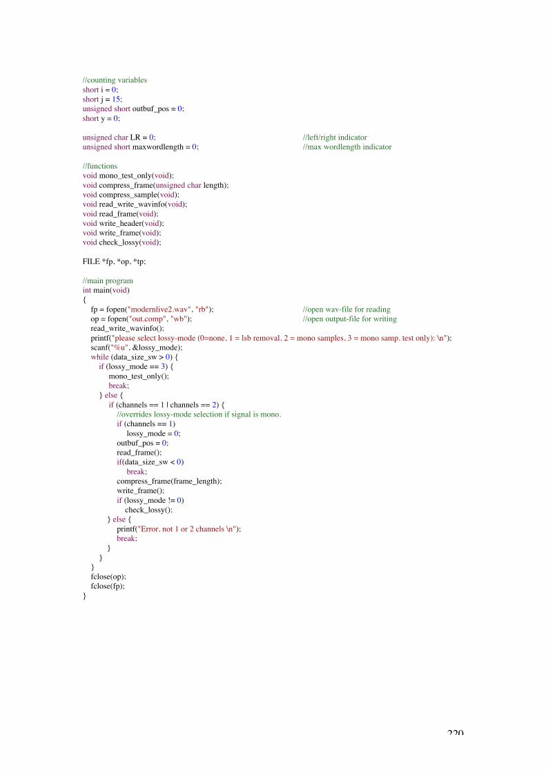
220

//counting variablesshort i = 0;short j = 15;unsigned short outbuf_pos = 0;short y = 0;

unsigned char LR = 0; //left/right indicatorunsigned short maxwordlength = 0; //max wordlength indicator

//functionsvoid mono_test_only(void);void compress_frame(unsigned char length);void compress_sample(void);void read_write_wavinfo(void);void read_frame(void);void write_header(void);void write_frame(void);void check_lossy(void);

FILE *fp, *op, *tp;

//main programint main(void) fp = fopen("modernlive2.wav", "rb"); //open wav-file for reading op = fopen("out.comp", "wb"); //open output-file for writing read_write_wavinfo(); printf("please select lossy-mode (0=none, 1 = lsb removal, 2 = mono samples, 3 = mono samp. test only): \n"); scanf("%u", &lossy_mode); while (data_size_sw > 0) if (lossy_mode == 3)

mono_test_only(); break;

else if (channels == 1 | channels == 2) //overrides lossy-mode selection if signal is mono. if (channels == 1)

lossy_mode = 0; outbuf_pos = 0; read_frame(); if(data_size_sw < 0)

break; compress_frame(frame_length); write_frame(); if (lossy_mode != 0) check_lossy();

else printf("Error, not 1 or 2 channels \n"); break;

fclose(op); fclose(fp);

221

//function that reads wav header and copies it to output filevoid read_write_wavinfo(void) // read wave header fread(id, sizeof(char), 4, fp); if(!strncmp(id, "RIFF", 4)) //if it is a RIFF, continue fwrite(id, sizeof(char), 4, op); fread(&size, sizeof(long), 1, fp); fwrite(&size, sizeof(long), 1, op); fread(id, sizeof(char), 4, fp); if(!strncmp(id, "WAVE", 4)) //If it is a WAVE, continue

fwrite(id, sizeof(char), 4, op); fread(id, sizeof(char), 4, fp); fwrite(id, sizeof(char), 4, op); fread(&format_length, sizeof(long), 1, fp); fwrite(&format_length, sizeof(long), 1, op); fread(&format_tag, sizeof(short), 1, fp); fwrite(&format_tag, sizeof(short), 1, op); fread(&channels_temp, sizeof(short), 1, fp); fwrite(&channels_temp, sizeof(short), 1, op); fread(&sample_rate, sizeof(long), 1, fp); fwrite(&sample_rate, sizeof(long), 1, op); fread(&avg_bytes_sec, sizeof(long), 1, fp); fwrite(&avg_bytes_sec, sizeof(long), 1, op); fread(&block_allign, sizeof(short), 1, fp); fwrite(&block_allign, sizeof(short), 1, op); fread(&bits_per_sample, sizeof(short), 1, fp); fwrite(&bits_per_sample, sizeof(short), 1, op); fread(id, sizeof(char), 4, fp); fwrite(id, sizeof(char), 4, op); fread(&data_size, sizeof(long), 1, fp); fwrite(&data_size, sizeof(long), 1, op);

else printf("Error: RIFF-file, but not a wave-file\n");

else printf("Error: not a RIFF-file\n");

//byteswapping of data_size since it is arranged with msbyte last data_size_sw = 0; data_size_sw = ((data_size&0x000000ff)<<24); data_size_sw = (data_size_sw|((data_size&0x0000ff00)<<8)); data_size_sw = (data_size_sw|((data_size&0x00ff0000)>>8)); data_size_sw = (data_size_sw|((data_size&0xff000000)>>24)); printf("Data size: %d \n", data_size_sw);

// byteswap channels variable channels = ((channels_temp & 0x00ff)<<8); channels = (channels | ((channels_temp & 0xff00)>>8));

//function that reads a frame of data and puts it in the input buffervoid read_frame(void) for(y=0; y<frame_length; y++) if(data_size_sw<0)

break; // read input value and change endian fread(&value_temp, sizeof(short), 1, fp); data_size_sw=data_size_sw-2; inputbuffer[y] = 0;

222

inputbuffer[y] = ((value_temp & 0x00ff)<<8); inputbuffer[y] = (inputbuffer[y] | ((value_temp & 0xff00)>>8)); //remove LSBs if lossy mode 1 if (lossy_mode == 1)

//convert to sign magnitude if (inputbuffer[y] < 0) inputbuffer[y] = (-inputbuffer[y]); i = 1; else i = 0;

//remove LSBs inputbuffer[y] = inputbuffer[y]>>lsb_rem; //back to twos complement if (i == 1)

inputbuffer[y]=(-inputbuffer[y]);

//function that handles compression of an entire framevoid compress_frame(unsigned char length) LR=0; // if lossy-mode is used, header must be included if (lossy_mode != 0) if (lossy_mode == 1)

header = lsb_rem; else if (lossy_mode == 2)

header = mono_samples; //8-bit header is used, //put header in output framebuffer for (i=8; i>0; i--)

if ((header & bittab[i-1]) != 0) out = out | bittab[j]; j--; if (j<0) outputbuffer[outbuf_pos] = out; outbuf_pos++; j=15; out = 0;

//if lossy mode is 0 or 1, compress entire frame if (lossy_mode != 2) for (y=0;y<length;y++)

compress_sample(); if (channels == 2) LR = !LR;

//if not compress some samples in mono (left chn. only)

else for (y=0;y<(length-mono_samples);y++)

compress_sample(); LR = !LR;

LR=0; y=(length-mono_samples); while(y<length)

compress_sample(); y=y+2;

223

//compression routinevoid compress_sample(void) //2nd order prediction residual = diff[LR] - diffprev[LR]; diffprev[LR] = diff[LR]; diff[LR] = inputbuffer[y] - valprev[LR]; valprev[LR] = inputbuffer[y];

// convert to sign-magnitude if (residual < 0) residual = (-residual); sign = 1; else sign = 0;

// perform Pod-coding

// find overflow overflow = 0; overflow = residual >> k[LR];

// find number of zeros numzeros = 0; // overflow can be max (18-k) bits for (i=0;i<(18-k[LR]);i++) if (overflow > (bittab[i]-1))

numzeros++; else

break;

// find max wordlength just to see how the coding performs if (((numzeros<<1)+k[LR]+1) > maxwordlength) maxwordlength = (numzeros<<1)+k[LR]+2;

// put together and write output data bit by bit // data fills the out-variable continuously from // MSB and downwards // using bit-table, bittable[j] is a 1 in position // j counting from LSB to MSB // when out-variable is filled (j<0), it starts // filling out a new one immideately

// sign if (sign != 0) out = out | bittab[j]; j--; if (j<0) outputbuffer[outbuf_pos] = out; outbuf_pos++; j=15; out = 0;

// zeros followed by overflow or just a one if the overflow is 0 if (numzeros == 0) out = out | bittab[j]; j--;

224

if (j<0) outputbuffer[outbuf_pos] = out; outbuf_pos++; j=15; out=0;

else //zeros for (i=numzeros; i>0; i--)

j--; if (j<0) outputbuffer[outbuf_pos] = out; outbuf_pos++; j=15; out=0;

// overflow for (i=numzeros; i>0; i--)

if ((overflow & bittab[i-1]) != 0) out = out | bittab[j]; j--; if (j<0) outputbuffer[outbuf_pos] = out; outbuf_pos++; j=15; out = 0;

// uncoded part (bit 1 to bit k of value) for (i=k[LR]; i>0; i--) if ((residual & bittab[i-1]) != 0) out = out | bittab[j]; j--; if (j<0) outputbuffer[outbuf_pos] = out; outbuf_pos++; j = 15; out = 0;

// calculate k for next sample N[LR]++; A[LR]+=residual; for (k[LR]=0; (N[LR]<<k[LR])<A[LR]; k[LR]++); // reset accumulation every frame if (N[LR]==255) N[LR]=0; A[LR]=0;

//function that writes the frame to filevoid write_frame(void) //write the frame output to file, since j is not reset, the remainder will be send in //the next write, this is for no-lossy or lossy-mode 1 for(y=0; y<outbuf_pos;y++) fwrite(&outputbuffer[y], sizeof(short), 1, op); outputbuffer[0] = outputbuffer[outbuf_pos+1];

225

// lossy mode check and calculationvoid check_lossy(void) //lsb_removal lossy mode if (lossy_mode == 1) // 80 because 128/80 is 10 bits pr. sample, which translates to ca 1Mbps if (outbuf_pos > 80)

// each word > 80 means 16 bits to much, to remove 1LSB from each sample in the //frame saves 128 bits, use shift to compensate //i.e. 128-sample frame => three left shift lsb_rem = (outbuf_pos-80)>>3;

else lsb_rem = 0;

//mono samples lossy mode if (lossy_mode == 2) if (outbuf_pos > 80)

//if n samples over 80, n samples must be sent in mono //since 1 sample is saved for each mono send //also make sure it's an even number to avoid mixing channels mono_samples = ((outbuf_pos-80)>>1)<<1;

else mono_samples = 0;

//mono test only routinevoid mono_test_only(void) tp = fopen("monotest.wav", "wb"); // read wave header fread(id, sizeof(char), 4, fp); //read in first four bytes if(!strncmp(id, "RIFF", 4)) //if it is a RIFF, continue fwrite(id, sizeof(char), 4, tp); fread(&size, sizeof(long), 1, fp); fwrite(&size, sizeof(long), 1, tp); fread(id, sizeof(char), 4, fp); if(!strncmp(id, "WAVE", 4)) //If it is a WAVE, continue

fwrite(id, sizeof(char), 4, tp); fread(id, sizeof(char), 4, fp); fwrite(id, sizeof(char), 4, tp); fread(&format_length, sizeof(long), 1, fp); fwrite(&format_length, sizeof(long), 1, tp); fread(&format_tag, sizeof(short), 1, fp); fwrite(&format_tag, sizeof(short), 1, tp); fread(&channels_temp, sizeof(short), 1, fp); fwrite(&channels_temp, sizeof(short), 1, tp); fread(&sample_rate, sizeof(long), 1, fp); fwrite(&sample_rate, sizeof(long), 1, tp); fread(&avg_bytes_sec, sizeof(long), 1, fp); fwrite(&avg_bytes_sec, sizeof(long), 1, tp); fread(&block_allign, sizeof(short), 1, fp); fwrite(&block_allign, sizeof(short), 1, tp); fread(&bits_per_sample, sizeof(short), 1, fp); fwrite(&bits_per_sample, sizeof(short), 1, tp); fread(id, sizeof(char), 4, fp); fwrite(id, sizeof(char), 4, tp); fread(&data_size, sizeof(long), 1, fp); fwrite(&data_size, sizeof(long), 1, tp);

else

226

printf("Error: RIFF-file, but not a wave-file\n"); else printf("Error: not a RIFF-file\n");

//byteswapping of data_size since it is arranged with msbyte last data_size_sw = 0; data_size_sw = ((data_size&0x000000ff)<<24); data_size_sw = (data_size_sw|((data_size&0x0000ff00)<<8)); data_size_sw = (data_size_sw|((data_size&0x00ff0000)>>8)); data_size_sw = (data_size_sw|((data_size&0xff000000)>>24)); printf("Data size: %d \n", data_size_sw);

// byteswap channels variable channels = ((channels_temp & 0x00ff)<<8); channels = (channels | ((channels_temp & 0xff00)>>8)); if (channels == 2) while(data_size_sw>0)

//write 40 stereo samples for (z=0;z<40;z++) if(data_size_sw <0) break; fread(&value_temp, sizeof(short), 1, fp); fwrite(&value_temp, sizeof(short),1,tp); data_size_sw = data_size_sw-2; if(data_size_sw<0) break; //and 24 mono samples per frame for(z=40;z<64;z++) if(data_size_sw<0)

break; fread(&value_temp, sizeof(short),2,fp); //write left input sample to left output fwrite(&value_temp, sizeof(short),1,tp); //and to right fwrite(&value_temp, sizeof(short),1,tp); data_size_sw = data_size_sw-4; z++;

else printf("Error, mono-mode test can only be done on stereo file"); fclose(tp);

/////////////////////////////////////////////////////////Hybrid lossless/lossy codec..…….////.........................……………….......////10 bit per sample output rate…….////LSB-removal or mono-samples.....////lossy-mode...................…………...////fixed 2nd order prediction.…….....////and Pod-encoding.............………..////.............................………………...////Written for Macintosh........……....////intel users, remove endian conv....////......................………………..........////decoder...........……………............////...................………………............////Ivar Løkken.............…………......////NTNU, 2004..........………....…...///////////////////////////////////////////////////////

227

#include <stdio.h>

// table for output bitshiftstatic unsigned long bittab[32] = 0x00000001,0x00000002,0x00000004,0x00000008,0x00000010,0x00000020,0x00000040,0x00000080, 0x00000100,0x00000200,0x00000400,0x00000800,0x00001000,0x00002000,0x00004000,0x00008000, 0x00010000,0x00020000,0x00040000,0x00080000,0x00100000,0x00200000,0x00400000,0x00800000, 0x01000000,0x02000000,0x04000000,0x08000000,0x10000000,0x20000000,0x40000000,0x80000000;

//table for 16-bit bitcheckstatic unsigned short bittabs[16] = 0x0001,0x0002,0x0004,0x0008,0x0010,0x0020,0x0040,0x0080, 0x0100,0x0200,0x0400,0x0800,0x1000,0x2000,0x4000,0x8000;

//outbut bufferlong outbuffer[128];

//wav header variableschar id[4];long size, data_size, data_size_sw;short format_tag, channels, channels_temp, block_allign, bits_per_sample;long format_length, sample_rate, avg_bytes_sec;

//lossy mode variablesunsigned char frame_length = 128; //frame lengthunsigned short header = 0; //header variableunsigned char lsb_rem = 0; //lsbs to be removed for a given frameunsigned char lsb_rem_last = 0; //same but from last frameunsigned int lossy_mode = 0; //lossy-mode variableunsigned char mono_samples=0; //number of mono samples

//read and write data variablesunsigned short in = 0; //input variablelong outvar = 0; //output variableshort PCMout_t = 0; //16-bit output datashort PCMout = 0; //16-bit output data right endianlong left = 0; //left channel variablelong right = 0; //right channel variable

//predictor variableslong residual = 0; //decoded residuallong diff[2] = 0,0; //calculated difference when 2nd orderlong out[2] = 0,0; //output variable

//decoder variablesunsigned short sign = 0; //sign-bitunsigned short numzeros=0; //number of zerosunsigned char k[2] = 6,6; //k-variable, compressed wordlength estimationunsigned long A[2] = 0,0; //accumulated value for calculation of kunsigned char N[2] = 0,0; //sample countunsigned char LR = 0; //channel indicator

//counting variablesshort i = 0; //counting variableunsigned char y = 0; //counting variableshort j = 15; //counting variablechar x = 0; //counting variable

//functionsvoid decompress_frame(unsigned char length);void decompress_sample(void);void read_write_wavinfo(void);void put_back_lsbs(void);void back_to_stereo(void);void write_frame_tofile(void);

228

FILE *fp, *op;

//main programint main(void) fp = fopen("out.comp", "rb"); //open wav-file for reading op = fopen("out.wav", "wb"); //open output-file for writing read_write_wavinfo();

//read first 16 bits fread(&in, sizeof(short), 1, fp); printf("please select lossy-mode (0=none, 1 = lsb removal, 2 = mono samples): \n"); scanf("%u", &lossy_mode); while(data_size_sw > 0) if (channels == 1 | channels == 2)

//overrides lossy mode selection if mono signal if (channels == 1) lossy_mode = 0; //decompress frame and check lossy modes decompress_frame(frame_length); if (lossy_mode == 1) put_back_lsbs(); else if (lossy_mode == 2) back_to_stereo(); //write output data to file write_frame_tofile();

else printf("Error, not 1 or 2 channels \n"); break;

fclose(fp); fclose(op);

//function that reads and writes data from wav headervoid read_write_wavinfo(void) if (fp) fread(id, sizeof(char), 4, fp); if(!strncmp(id, "RIFF", 4)) //if it is a RIFF, continue fwrite(id, sizeof(char), 4, op); fread(&size, sizeof(long), 1, fp); fwrite(&size, sizeof(long), 1, op); fread(id, sizeof(char), 4, fp); if(!strncmp(id, "WAVE", 4)) //If it is a WAVE, continue fwrite(id, sizeof(char), 4, op); fread(id, sizeof(char), 4, fp); fwrite(id, sizeof(char), 4, op); fread(&format_length, sizeof(long), 1, fp); fwrite(&format_length, sizeof(long), 1, op); fread(&format_tag, sizeof(short), 1, fp); fwrite(&format_tag, sizeof(short), 1, op); fread(&channels_temp, sizeof(short), 1, fp); fwrite(&channels_temp, sizeof(short), 1, op); fread(&sample_rate, sizeof(long), 1, fp); fwrite(&sample_rate, sizeof(long), 1, op); fread(&avg_bytes_sec, sizeof(long), 1, fp); fwrite(&avg_bytes_sec, sizeof(long), 1, op); fread(&block_allign, sizeof(short), 1, fp); fwrite(&block_allign, sizeof(short), 1, op); fread(&bits_per_sample, sizeof(short), 1, fp); fwrite(&bits_per_sample, sizeof(short), 1, op);

229

fread(id, sizeof(char), 4, fp); fwrite(id, sizeof(char), 4, op); fread(&data_size, sizeof(long), 1, fp); fwrite(&data_size, sizeof(long), 1, op); else printf("Error: RIFF-file, but not a wave-file\n"); else printf("Error: not a RIFF-file\n");

//byteswapping of data_size since it is arranged with msbyte last data_size_sw = 0; data_size_sw = ((data_size&0x000000ff)<<24); data_size_sw = (data_size_sw|((data_size&0x0000ff00)<<8)); data_size_sw = (data_size_sw|((data_size&0x00ff0000)>>8)); data_size_sw = (data_size_sw|((data_size&0xff000000)>>24)); printf("Data size: %d \n", data_size_sw); // byteswap channels variable channels = ((channels_temp & 0x00ff)<<8); channels = (channels | ((channels_temp & 0xff00)>>8));

//function that handles decompression of one framevoid decompress_frame(unsigned char length) //if lossy-mode is used, header is included if (lossy_mode != 0) // read frame header header = 0; for(i=8;i>0;i--)

if((in & bittabs[j]) != 0) header = header | bittabs[i-1]; j--; if (j<0) fread(&in, sizeof(short), 1, fp); j = 15;

//header content is put in right variable if (lossy_mode == 1)

lsb_rem_last = lsb_rem; lsb_rem = header;

else if (lossy_mode == 2) mono_samples = header;

LR = 0; // decompress the samples in the frame if (lossy_mode != 2) for (y=0;y<length;y++)

decompress_sample(); if (channels == 2) LR = !LR;

//if mono-mode, decompress stereo samples first, then mono samples else y=0; for (y=0;y<(length-mono_samples);y++)

decompress_sample(); LR = !LR;

230

LR = 0; y=(length-mono_samples); while (y<length)

decompress_sample(); y=y+2;

//decompression routinevoid decompress_sample(void) // read sign sign = in & bittabs[j]; j--; if (j<0) fread(&in, sizeof(short), 1, fp); j = 15;

// count zeros numzeros = 0; while ((in & bittabs[j]) == 0) numzeros++; j--; if (j<0)

fread(&in, sizeof(short), 1, fp); j = 15;

// if numzeros = 0, skip the "1" prefix if (numzeros == 0) j--; if (j<0)

fread(&in, sizeof(short), 1, fp); j = 15;

// read the next part (numzeros and k bits) bit by bit and construct output residual = 0; for (i=(numzeros+k[LR]) ; i>0; i--) if ((in & bittabs[j]) != 0)

residual = residual | bittab[i-1]; j--; if (j<0)

fread(&in, sizeof(short), 1, fp); j = 15;

// calculate k for next sample N[LR]++; A[LR] += residual; for (k[LR]=0; (N[LR]<<k[LR])<A[LR]; k[LR]++);

// reset accumulation every 255th sample if (N[LR]==255) N[LR]=0; A[LR]=0;

// restore sign representation if (sign != 0) residual = -residual;

231

residual = residual; // construct output data, depending on prediction order used diff[LR] += residual; out[LR] += diff[LR]; outbuffer[y] = out[LR];

//routine to correct amplitude if LSBs have been removed//convert to sign-magnitude and put back LSBs//lsb_rem_last for the first two samples, since prediction//gives a two-sample delay (from residual n to sample n)//which must be alligned with the LSB-removalvoid put_back_lsbs(void) for(y=0;y<frame_length;y++) if(outbuffer[y]<0)

outbuffer[y] = (-outbuffer[y]); i = 1;

else i = 0;

if (y == 0 | y == 1)

outbuffer[y] = outbuffer[y]<<lsb_rem_last; else

outbuffer[y] = outbuffer[y]<<lsb_rem; if (i == 1)

outbuffer[y] = -outbuffer[y];

//function to produce stereo output if mono-mode is used//same compensation for delay as in put_back_lsbvoid back_to_stereo(void) outbuffer[1] = outbuffer[0] y = (frame_length-mono_samples)+2;

while(y<frame_length)outbuffer[y+1] = outbuffer[y];y = y+2;

//write output data to filevoid write_frame_tofile(void) for(y=0;y<frame_length;y++) outvar = outbuffer[y]; //limit value if (outvar > 32767)

outvar = 32767; if (outvar < -32768)

outvar = -32768; PCMout_t = outvar; // convert back to big endian PCMout = ((PCMout_t & 0x00ff)<<8); PCMout = (PCMout | ((PCMout_t & 0xff00)>>8)); // write output value fwrite(&PCMout, sizeof(short), 1, op); data_size_sw = data_size_sw - 2;

232

Dropped packet simulator///////////////////////////////////////////////////File that emulates dropped.….////packets and different ways....////of handling to see how it…...////affects audio quality....……...////....................…………............////Ivar L√∏kken, NTNU 2004./////////////////////////////////////////////////

#include <stdio.h>#include <math.h>

void read_write_wavinfo(void); //read and write wav headervoid run_with_drop(void); //run with packet lossvoid run_no_drop(void); //run without packet loss

//wav-header data variableschar id[4];long size, data_size, data_size_sw;short format_tag, channels, channels_temp, block_allign, bits_per_sample;long format_length, sample_rate, avg_bytes_sec;

//audio data variablesshort last_packet[256]; //buffer last packet in case of repeatshort value = 0; //value inshort silence = 0x8000; //silence variable

//parameter variablesunsigned int packet_length = 0; //length of packet in samplesunsigned int drop_interval = 0; //how often packets are droppedunsigned int lost_in_a_row = 0; //how many packets are lost in a rowunsigned int handling_mode = 0; //how to handle lost packetsunsigned int losson = 0; //packet loss on/off indicator

//counting variablesshort i = 0;short j = 0;

FILE *fp, *op;

//main programint main(void) fp = fopen("modernlive.wav", "rb"); //open wav-file for reading op = fopen("out.wav", "wb"); //open output-file for writing read_write_wavinfo(); //read wav-header printf("\nDo you want packets to be lost (0=no, 1=yes): "); scanf("%u", &losson); if (losson)

//select parametersprintf("\nPlease select packet length in samples (max 256): ");scanf("%u", &packet_length);printf("\nPlease select packet drop interval: ");scanf("%u", &drop_interval);printf("\nPlease select how many packets should be dropped each time (default = 1): ");scanf("%u", &lost_in_a_row);printf("\nPlease select handling mode (1 = insert silence, 2 = repeat last OK packet): ");scanf("%u", &handling_mode);//runrun_with_drop();

else //run with no packet loss

233

run_no_drop();

//function that reads wav header and copies it to output filevoid read_write_wavinfo(void) // read wave header fread(id, sizeof(char), 4, fp); if(!strncmp(id, "RIFF", 4)) //if it is a RIFF, continue

fwrite(id, sizeof(char), 4, op);fread(&size, sizeof(long), 1, fp);fwrite(&size, sizeof(long), 1, op);fread(id, sizeof(char), 4, fp);if(!strncmp(id, "WAVE", 4)) //If it is a WAVE, continue fwrite(id, sizeof(char), 4, op); fread(id, sizeof(char), 4, fp); fwrite(id, sizeof(char), 4, op); fread(&format_length, sizeof(long), 1, fp); fwrite(&format_length, sizeof(long), 1, op); fread(&format_tag, sizeof(short), 1, fp); fwrite(&format_tag, sizeof(short), 1, op); fread(&channels_temp, sizeof(short), 1, fp); fwrite(&channels_temp, sizeof(short), 1, op); fread(&sample_rate, sizeof(long), 1, fp); fwrite(&sample_rate, sizeof(long), 1, op); fread(&avg_bytes_sec, sizeof(long), 1, fp); fwrite(&avg_bytes_sec, sizeof(long), 1, op); fread(&block_allign, sizeof(short), 1, fp); fwrite(&block_allign, sizeof(short), 1, op); fread(&bits_per_sample, sizeof(short), 1, fp); fwrite(&bits_per_sample, sizeof(short), 1, op); fread(id, sizeof(char), 4, fp); fwrite(id, sizeof(char), 4, op); fread(&data_size, sizeof(long), 1, fp); fwrite(&data_size, sizeof(long), 1, op); else printf("Error: RIFF-file, but not a wave-file\n");

else printf("Error: not a RIFF-file\n");

//byteswapping of data_size since it is arranged with msbyte last data_size_sw = 0; data_size_sw = ((data_size&0x000000ff)<<24); data_size_sw = (data_size_sw|((data_size&0x0000ff00)<<8)); data_size_sw = (data_size_sw|((data_size&0x00ff0000)>>8)); data_size_sw = (data_size_sw|((data_size&0xff000000)>>24)); printf("Data size: %d \n", data_size_sw);

// byteswap channels variable channels = ((channels_temp & 0x00ff)<<8); channels = (channels | ((channels_temp & 0xff00)>>8));

//function that reads and writes data with packet lossvoid run_with_drop(void) while (data_size_sw > 0)

//read and write the packets that shall not be lostfor (i=0;i<(drop_interval-lost_in_a_row);i++) for (j=0;j<packet_length;j++)

fread(&value, sizeof(short), 1, fp);fwrite(&value, sizeof(short),1,op);

234

//back up last packet in case of repetition mode selectedlast_packet[j] = value;data_size_sw = data_size_sw - 2;if (data_size_sw<0) break;

if (data_size_sw<0) break;//dropped packetsfor (i=(drop_interval-lost_in_a_row);i<drop_interval;i++) for (j=0;j<packet_length;j++)

//if handling mode 1, write silence to output fileif (handling_mode==1) fread(&value, sizeof(short), 1, fp); fwrite(&silence, sizeof(short),1,op);

data_size_sw = data_size_sw - 2; if (data_size_sw<0) break; //if handling mode 2, write last OK packet to output file

else if (handling_mode == 2) fread(&value, sizeof(short), 1, fp); fwrite(&last_packet[j], sizeof(short),1,op); data_size_sw = data_size_sw - 2; if (data_size_sw<0) break;

if (data_size_sw<0) break;

fclose(fp); fclose(op);

//function that reads and writes data with no lossvoid run_no_drop(void) while (data_size_sw > 0)

fread(&value, sizeof(short), 1, fp);fwrite(&value, sizeof(short),1,op);data_size_sw = data_size_sw - 2;

fclose(fp); fclose(op);

235

Appendix 7. MatLab ScriptsPrediction w. selectable filter and resulting entropycalculationfunction [ErLeft, ErRight]=decorr(path, B, A)%Matlab-function for intra-channel decorrelation of wavfile.%The function plots histogram and calculates entropy%%FIR- or IIR-filters of any order may be used%%Designed for two-channel 16-bit wavefile%%[error_left, error_right]=diffdecorr('c:\path\filename.wav', B, A)%%B and A are filter coefficients%a(1)*y(n) = b(1)*x(n) + b(2)*x(n-1) + ... + b(nb+1)*x(n-nb)% - a(2)*y(n-1) - ... - a(na+1)*y(n-na)%%Made by: Ivar Løkken, 19/1-04

signal=wavread(path);samples=signal*(2^15-1);%Removes normalization of wavefile.%The function Wavread normalizes sample values to [-1 1]%actual sample values for 16-bits is [-32767 32767]

vector=samples(:);%Puts the two channels in one vector

LCH=vector(1:length(vector)/2);RCH=vector(length(vector)/2+1:length(vector));%separates left channel from right

ErLCH=filter(B,A,LCH);ErRCH=filter(B,A,RCH);%calculates prediction error

subplot(2,1,1);hist(ErLCH,min(ErLCH):max(ErLCH));title('Histogram, predicted error Left Channel');ylabel('Number of occurances');xlabel('sample value');subplot(2,1,2);hist(ErRCH,min(ErRCH):max(ErRCH));title('Histogram, predicted error Right Channel');ylabel('Number of occurances');xlabel('sample value');%plots normalized histograms

histoL=hist(ErLCH,min(ErLCH):max(ErLCH));probsL=histoL/sum(histoL);histoR=hist(ErRCH,min(ErRCH):max(ErRCH));probsR=histoR/sum(histoR);%generates probability distribution based on histogram

IL=-log2(probsL);IL(IL==-Inf) = 0;IL(IL==Inf) = 0;prodL=probsL.*IL;ErLeft=sum(prodL);

IR=-log2(probsR);

236

IR(IR==-Inf) = 0;IR(IR==Inf) = 0;prodR=probsR.*IR;ErRight=sum(prodR);%Calculates entropy using standard formula

Wavfile entropy calculatorfunction [Left, Right]=entropy(path)%Matlab-function for calculation of entropy.%Designed for two-channel 16-bit wavefile%%%Calculates entropy for left and right channel separatly%[left, right]=entropy('c:\path\filename.wav')%%Made by: Ivar Løkken, 14/1-04

signal=wavread(path);samples=signal*(2^15-1);%Removes normalization of wavefile.%The function Wavread normalizes sample values to [-1 1]%actual sample values for 16-bits is [-32767 32767]

vector=samples(:);%Puts the two channels in one vector

LCH=vector(1:length(vector)/2);RCH=vector(length(vector)/2+1:length(vector));%separates left channel from right

histoL=hist(LCH,min(LCH):max(LCH));probsL=histoL/sum(histoL);histoR=hist(RCH,min(RCH):max(RCH));probsR=histoR/sum(histoR);%generates probability distribution based on histogram

IL=-log2(probsL);IL(IL==-Inf) = 0;IL(IL==Inf) = 0;prodL=probsL.*IL;Left=sum(prodL);

IR=-log2(probsR);IR(IR==-Inf) = 0;IR(IR==Inf) = 0;prodR=probsR.*IR;Right=sum(prodR);%Calculates entropy using standard formula

237

Lossy compression error calculatorfunction [PCMerror, SER] = errorcal(infile, outfile)

%%%%%%%%%%%%%%%%%%%%%%Funtion that calculates SER and............%%error rate for lossy compression...….....%%.......................................……………....%%Ivar Løkken, NTNU 2002.............…....%%%%%%%%%%%%%%%%%%%%%%%[Error, SER] = errorcal(infile, outfile)..%%.......................................……………....%%%%%%%%%%%%%%%%%%%%%%

in_t = wavread(infile);compfile_t = wavread(outfile);

if size(in_t)<size(compfile_t) siz = size(in_t);else siz = size(compfile_t);endin = in_t(1:siz);compfile = compfile_t(1:siz);

%SER and absolute maximum errorerror = in-compfile;errorones = ones(siz);inpower = (1/(2*siz+1))*(errorones)'*(in.*in);errorpower = (1/(2*siz+1))*(errorones)'*(error.*error);SER = 10*log(inpower/errorpower);PCMerror = (max(abs(error))/max(abs(in)));

subplot(3,1,1), plot(in);title('Input (normalised & quantised)');subplot(3,1,2), plot(compfile);title('Output');subplot(3,1,3), plot(error);title('Error');s=sprintf('SNR = %4.1fdB\n', SER);text(0.5,-90,s);s=sprintf('Max absolute error (normalized) = %4.1fdB\n', PCMerror);text(0.5,-110,s);

function centroid=speccent(path)

238

Spectral centroid calculator%function for calculating spectral centroid of wav-file%%Ivar Løkken%%centroid=speccent(path)%where path is wavefile path,%for instance. 'c:\music\file.wav'

%read signal[signal, FS, NBITS] = wavread(path);N=length(signal)+1;

%do FFT and plot it

FT=abs(fft(signal));

%perform antialiasing (energy above FS/2 must be removed)FTfilt=FT(1:N/2);

%plot filtered FFT from 0 to FS/2fftDB=db(FTfilt);freq=[0:FS/N:FS*(1-1/N)/2];plot(freq, fftDB);title('FFT and spectral centroid of wavfile');ylabel('Amplitude, dB');xlabel('Frequency, HZ');grid;

%calculate centroidsumFA=0;sumA=0;for i=1:N/2 sumFA=sumFA+i*FTfilt(i); sumA=sumA+FTfilt(i); i=i+1;endcent=sumFA/sumA;

%convert to correct frequency scalecentroid=cent*(FS/(2*N));s=sprintf('Spectral centroid = %4.1fHZ\n', centroid);text(4000,40,s);

239

Appendix 8. Tools Used During DevelopmentHardwareApple Powerbook G4, 1Ghz/512Mb/40Gb/12”, running Mac OS-X 10.3 ”Panther”and Windows 2000 SP4 through Virtual PC 6.Toshiba Satelite 4070CDS Celeron, 366Mhz/192Mb/4Gb/13”, running Windows2000 SP4.Eizo FlexScan F57 external 17” CRT-monitor.The WLS hardware developed as part of this thesis.

Software

General programming: Xcode Tools v.1.1 for OS-X.Schematics design: DesignWorks Lite 4.5 for OS-X.Calculations, testing: Mathworks MatLab 6.5 for Unix/OS-X.Analog simulations: AimSpice 3.8 for Windows, MacInit Mi-Sugar 0.5.2 for OS-X.Chart and diagram drawings: The Omni Group OmniGraffle for OS-X.MCU-programming: SDCC microcontroller compiler for UNIX/OS-X.CC2400-setup: Chipcon SmartLink RF for Windows.General documentation: Microsoft Office-X for OS-X.