2021 Load Forecast Supplement - PJM

PJM © 2020

2021 Load Forecast Supplement

PJM Resource Adequacy Planning Department

January 2021

For Public Use


PJM © 2020 www.pjm.com | For Public Use i | P a g e

This page is intentionally left blank

https://www.pjm.com/


PJM © 2020 www.pjm.com | For Public Use ii | P a g e

Contents I. Introduction and Overview............................................................................................................................ 1

II. Sector Models and Use Indexes ................................................................................................................... 1

A. Residential............................................................................................................................................ 2

1. Residential – Customers ............................................................................................................................ 2 2. Residential – Average Use per Customer .................................................................................................. 2 3. Residential – Total Use .............................................................................................................................. 6

B. Commercial .......................................................................................................................................... 6

1. Commercial – Pre-process ......................................................................................................................... 7 2. Commercial – Drivers ................................................................................................................................. 8 3. Commercial – Model .................................................................................................................................. 8

C. Industrial ............................................................................................................................................... 9

D. Use Indexes ....................................................................................................................................... 10

III. Non-Weather Sensitive Load ...................................................................................................................... 11

A. Establish History ................................................................................................................................. 11

B. Establish Forecast .............................................................................................................................. 12

IV. Weather Variables ........................................................................................................................................ 12

A. Heating and Cooling ........................................................................................................................... 13

B. Cloud Cover ....................................................................................................................................... 15

V. Final Forecast Model ................................................................................................................................... 16

A. Model Specification ............................................................................................................................ 16

B. Forecast Processing ........................................................................................................................... 18

1. Non-Coincident Peaks .............................................................................................................................. 18 2. Coincident Peaks ..................................................................................................................................... 19 3. Energy ...................................................................................................................................................... 19

VI. Distributed Solar Generation ...................................................................................................................... 20

A. Historical Data - PJM EIS and GATS ................................................................................................. 20

B. Approach to Including in Forecast ...................................................................................................... 20

1. Step One: Incorporating historical estimates of distributed solar ............................................................. 20 2. Step Two: Incorporating historical estimates of distributed solar ............................................................. 21

VII. Plug-in Electric Vehicles ............................................................................................................................. 21

VIII. Forecast Adjustments ................................................................................................................................. 22

A. APS .................................................................................................................................................... 22

B. BGE .................................................................................................................................................... 22



PJM © 2020 www.pjm.com | For Public Use iii | P a g e

C. COMED .............................................................................................................................................. 23

D. Dominion (VEPCO) ............................................................................................................................ 23

IX. Calendar Variables ...................................................................................................................................... 24

X. Economics Zonal Assignment.................................................................................................................... 27

XI. End-Use Inputs ............................................................................................................................................ 28

A. Residential.......................................................................................................................................... 28

1. Efficiency of Residential Cooling Equipment ............................................................................................ 30 B. Commercial ........................................................................................................................................ 30

XII. Additional Materials ..................................................................................................................................... 31


Type Doc Title

PJM © 2020 www.pjm.com | For Public Use 1 | P a g e

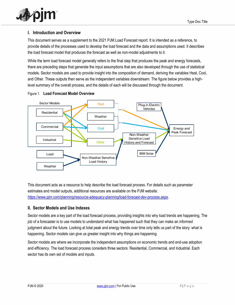
I. Introduction and Overview This document serves as a supplement to the 2021 PJM Load Forecast report. It is intended as a reference, to provide details of the processes used to develop the load forecast and the data and assumptions used. It describes the load forecast model that produces the forecast as well as non-model adjustments to it.

While the term load forecast model generally refers to the final step that produces the peak and energy forecasts, there are preceding steps that generate the input assumptions that are also developed through the use of statistical models. Sector models are used to provide insight into the composition of demand, deriving the variables Heat, Cool, and Other. These outputs then serve as the independent variables downstream. The figure below provides a high-level summary of the overall process, and the details of each will be discussed through the document.

Figure 1. Load Forecast Model Overview

This document acts as a resource to help describe the load forecast process. For details such as parameter estimates and model outputs, additional resources are available on the PJM website: https://www.pjm.com/planning/resource-adequacy-planning/load-forecast-dev-process.aspx.

II. Sector Models and Use Indexes Sector models are a key part of the load forecast process, providing insights into why load trends are happening. The job of a forecaster is to use models to understand what has happened such that they can make an informed judgment about the future. Looking at total peak and energy trends over time only tells us part of the story: what is happening. Sector models can give us greater insight into why things are happening.

Sector models are where we incorporate the independent assumptions on economic trends and end-use adoption and efficiency. The load forecast process considers three sectors: Residential, Commercial, and Industrial. Each sector has its own set of models and inputs.


https://www.pjm.com/planning/resource-adequacy-planning/load-forecast-dev-process.aspx



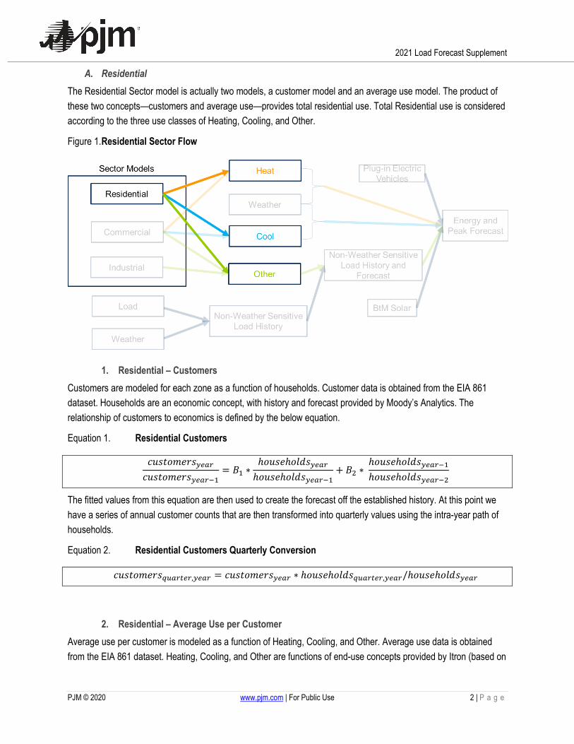
A. Residential The Residential Sector model is actually two models, a customer model and an average use model. The product of these two concepts—customers and average use—provides total residential use. Total Residential use is considered according to the three use classes of Heating, Cooling, and Other.

Figure 1. Residential Sector Flow

1. Residential – Customers Customers are modeled for each zone as a function of households. Customer data is obtained from the EIA 861 dataset. Households are an economic concept, with history and forecast provided by Moody’s Analytics. The relationship of customers to economics is defined by the below equation.

Equation 1. Residential Customers

𝑐𝑐𝑐𝑐𝑐𝑐𝑐𝑐𝑐𝑐𝑐𝑐𝑐𝑐𝑐𝑐𝑐𝑐𝑦𝑦𝑦𝑦𝑦𝑦𝑦𝑦𝑐𝑐𝑐𝑐𝑐𝑐𝑐𝑐𝑐𝑐𝑐𝑐𝑐𝑐𝑐𝑐𝑐𝑐𝑦𝑦𝑦𝑦𝑦𝑦𝑦𝑦−1

= 𝐵𝐵1 ∗ℎ𝑐𝑐𝑐𝑐𝑐𝑐𝑐𝑐ℎ𝑐𝑐𝑜𝑜𝑜𝑜𝑐𝑐𝑦𝑦𝑦𝑦𝑦𝑦𝑦𝑦ℎ𝑐𝑐𝑐𝑐𝑐𝑐𝑐𝑐ℎ𝑐𝑐𝑜𝑜𝑜𝑜𝑐𝑐𝑦𝑦𝑦𝑦𝑦𝑦𝑦𝑦−1

+ 𝐵𝐵2 ∗ ℎ𝑐𝑐𝑐𝑐𝑐𝑐𝑐𝑐ℎ𝑐𝑐𝑜𝑜𝑜𝑜𝑐𝑐𝑦𝑦𝑦𝑦𝑦𝑦𝑦𝑦−1ℎ𝑐𝑐𝑐𝑐𝑐𝑐𝑐𝑐ℎ𝑐𝑐𝑜𝑜𝑜𝑜𝑐𝑐𝑦𝑦𝑦𝑦𝑦𝑦𝑦𝑦−2

The fitted values from this equation are then used to create the forecast off the established history. At this point we have a series of annual customer counts that are then transformed into quarterly values using the intra-year path of households.

Equation 2. Residential Customers Quarterly Conversion

𝑐𝑐𝑐𝑐𝑐𝑐𝑐𝑐𝑐𝑐𝑐𝑐𝑐𝑐𝑐𝑐𝑐𝑐𝑞𝑞𝑞𝑞𝑦𝑦𝑦𝑦𝑞𝑞𝑦𝑦𝑦𝑦,𝑦𝑦𝑦𝑦𝑦𝑦𝑦𝑦 = 𝑐𝑐𝑐𝑐𝑐𝑐𝑐𝑐𝑐𝑐𝑐𝑐𝑐𝑐𝑐𝑐𝑐𝑐𝑦𝑦𝑦𝑦𝑦𝑦𝑦𝑦 ∗ ℎ𝑐𝑐𝑐𝑐𝑐𝑐𝑐𝑐ℎ𝑐𝑐𝑜𝑜𝑜𝑜𝑐𝑐𝑞𝑞𝑞𝑞𝑦𝑦𝑦𝑦𝑞𝑞𝑦𝑦𝑦𝑦,𝑦𝑦𝑦𝑦𝑦𝑦𝑦𝑦/ℎ𝑐𝑐𝑐𝑐𝑐𝑐𝑐𝑐ℎ𝑐𝑐𝑜𝑜𝑜𝑜𝑐𝑐𝑦𝑦𝑦𝑦𝑦𝑦𝑦𝑦

2. Residential – Average Use per Customer Average use per customer is modeled as a function of Heating, Cooling, and Other. Average use data is obtained from the EIA 861 dataset. Heating, Cooling, and Other are functions of end-use concepts provided by Itron (based on




data from the EIA’s Annual Energy Outlook) and economic concepts that are provided by Moody’s Analytics. The relationship of average use to Heating (xheat), Cooling (xcool), and Other (xother) is defined by the below equation.

Equation 3. Residential Average Use

𝑐𝑐𝑐𝑐𝑐𝑐𝑦𝑦𝑦𝑦𝑦𝑦𝑦𝑦 = 𝐵𝐵0 ∗ 𝑥𝑥ℎ𝑐𝑐𝑒𝑒𝑐𝑐𝑦𝑦𝑦𝑦𝑦𝑦𝑦𝑦 + 𝐵𝐵1 ∗ 𝑥𝑥𝑐𝑐𝑐𝑐𝑐𝑐𝑜𝑜𝑦𝑦𝑦𝑦𝑦𝑦𝑦𝑦 + 𝐵𝐵2 ∗ 𝑥𝑥𝑐𝑐𝑐𝑐ℎ𝑐𝑐𝑐𝑐𝑦𝑦𝑦𝑦𝑦𝑦𝑦𝑦 + 𝐴𝐴𝐴𝐴(1)

The table below provides a list of residential end-uses and indicates how they are allocated to Heating, Cooling, and Other. For each end-use, data provided by Itron includes saturation (% of customers with device), efficiency (relative efficiency of device), and intensity (use per device accounting for saturation and efficiency).

Table 1. List of Residential End-Uses and Assignment

Bucket Use Type Definition

Heating EFurn Electric furnace and resistant room space heaters

Heating HPHeat Heat pump space heating

Heating GHPHeat Ground-source heat pump space heating

Heating SecHt Secondary heating

Cooling CAC Central air conditioning

Cooling HPCool Heat pump space cooling

Cooling GHPCool Ground-source heat pump space cooling

Cooling RAC Room air conditioners

Other EWHeat Electric water heating

Other ECook Electric cooking

Other Ref1 Refrigerator

Other Ref2 Second refrigerator

Other Frz Freezer

Other Dish Dishwasher

Other CWash Electric clothes washer

Other EDry Electric clothes dryer

Other TV TV sets

Heating FurnFan Furnace fans

Other Light Lighting

Other Misc Miscellaneous electric appliances




Heating (xheat) is a function of heating end-uses as identified in the above table with adjustments for weather, income per household, population per household, and building shell efficiency.

Equation 4. Residential Heating Variable (xheat)

𝑥𝑥ℎ𝑐𝑐𝑒𝑒𝑐𝑐𝑦𝑦𝑦𝑦𝑦𝑦𝑦𝑦 = 𝑐𝑐𝑒𝑒𝑐𝑐_ℎ𝑐𝑐𝑒𝑒𝑐𝑐𝑦𝑦𝑦𝑦𝑦𝑦𝑦𝑦 ∗ ℎ𝑜𝑜𝑜𝑜_𝑖𝑖𝑛𝑛𝑦𝑦𝑦𝑦𝑦𝑦𝑦𝑦

Where

𝑐𝑐𝑒𝑒𝑐𝑐_ℎ𝑐𝑐𝑒𝑒𝑐𝑐𝑦𝑦𝑦𝑦𝑦𝑦𝑦𝑦 = 𝐸𝐸𝐸𝐸𝑐𝑐𝑐𝑐𝑛𝑛𝑦𝑦𝑦𝑦𝑦𝑦𝑦𝑦 +𝐻𝐻𝐻𝐻𝐻𝐻𝑐𝑐𝑒𝑒𝑐𝑐𝑦𝑦𝑦𝑦𝑦𝑦𝑦𝑦 + 𝐺𝐺𝐻𝐻𝐻𝐻𝐻𝐻𝑐𝑐𝑒𝑒𝑐𝑐𝑦𝑦𝑦𝑦𝑦𝑦𝑦𝑦 + 𝑆𝑆𝑐𝑐𝑐𝑐𝐻𝐻𝑐𝑐𝑦𝑦𝑦𝑦𝑦𝑦𝑦𝑦 + 𝐸𝐸𝑐𝑐𝑐𝑐𝑛𝑛𝐸𝐸𝑒𝑒𝑛𝑛𝑦𝑦𝑦𝑦𝑦𝑦𝑦𝑦

and

ℎ𝑜𝑜𝑜𝑜_𝑖𝑖𝑛𝑛𝑦𝑦𝑦𝑦𝑦𝑦𝑦𝑦 =ℎ𝑜𝑜𝑜𝑜𝑦𝑦𝑦𝑦𝑦𝑦𝑦𝑦ℎ𝑜𝑜𝑜𝑜1998

Each of EFurn, HPHeat, GHPHeat, SecHt, and FurnFan are additionally multiplied by the following:

�𝐻𝐻𝑐𝑐𝑃𝑃𝑐𝑐𝑜𝑜𝑒𝑒𝑐𝑐𝑖𝑖𝑐𝑐𝑛𝑛_𝑃𝑃𝑐𝑐𝑐𝑐_ℎ𝑐𝑐𝑐𝑐𝑐𝑐𝑐𝑐ℎ𝑐𝑐𝑜𝑜𝑜𝑜𝑦𝑦𝑦𝑦𝑦𝑦𝑦𝑦�𝑥𝑥 ∗ �𝐼𝐼𝑛𝑛𝑐𝑐𝑐𝑐𝑐𝑐𝑐𝑐_𝑃𝑃𝑐𝑐𝑐𝑐_ℎ𝑐𝑐𝑐𝑐𝑐𝑐𝑐𝑐ℎ𝑐𝑐𝑜𝑜𝑜𝑜𝑦𝑦𝑦𝑦𝑦𝑦𝑦𝑦�

𝑦𝑦 ∗ 𝑆𝑆𝑐𝑐𝑐𝑐𝑐𝑐𝑐𝑐𝑐𝑐𝑐𝑐𝑐𝑐𝑒𝑒𝑜𝑜_𝐻𝐻𝑐𝑐𝑒𝑒𝑐𝑐𝑖𝑖𝑛𝑛𝑔𝑔𝑦𝑦𝑦𝑦𝑦𝑦𝑦𝑦

Where x and y are elasticities provided by Itron and Structural_Heating is a measure of building size adjusted for relative building shell efficiency.

Cooling (xcool) is a function of cooling end-uses as identified in the above table with adjustments for weather, income per household, population per household, and building shell efficiency.

Equation 5. Residential Cooling Variable (xcool)

𝑥𝑥𝑐𝑐𝑐𝑐𝑐𝑐𝑜𝑜𝑦𝑦𝑦𝑦𝑦𝑦𝑦𝑦 = 𝑐𝑐𝑒𝑒𝑐𝑐_𝑐𝑐𝑐𝑐𝑐𝑐𝑜𝑜𝑦𝑦𝑦𝑦𝑦𝑦𝑦𝑦 ∗ 𝑐𝑐𝑜𝑜𝑜𝑜_𝑖𝑖𝑛𝑛𝑦𝑦𝑦𝑦𝑦𝑦𝑦𝑦

Where

𝑐𝑐𝑒𝑒𝑐𝑐_𝑐𝑐𝑐𝑐𝑐𝑐𝑜𝑜𝑦𝑦𝑦𝑦𝑦𝑦𝑦𝑦 = 𝐶𝐶𝐴𝐴𝐶𝐶𝑌𝑌𝑦𝑦𝑦𝑦𝑦𝑦 + 𝐻𝐻𝐻𝐻𝐶𝐶𝑐𝑐𝑐𝑐𝑜𝑜𝑦𝑦𝑦𝑦𝑦𝑦𝑦𝑦 + 𝐺𝐺𝐻𝐻𝐻𝐻𝐶𝐶𝑐𝑐𝑐𝑐𝑜𝑜𝑦𝑦𝑦𝑦𝑦𝑦𝑦𝑦 + 𝐴𝐴𝐴𝐴𝐶𝐶𝑦𝑦𝑦𝑦𝑦𝑦𝑦𝑦

and

𝑐𝑐𝑜𝑜𝑜𝑜_𝑖𝑖𝑛𝑛𝑦𝑦𝑦𝑦𝑦𝑦𝑦𝑦 =𝑐𝑐𝑜𝑜𝑜𝑜𝑦𝑦𝑦𝑦𝑦𝑦𝑦𝑦𝑐𝑐𝑜𝑜𝑜𝑜1998

Each of CAC, HPCool, GHPCool, and RAC are additionally multiplied by the following:


𝑦𝑦 ∗ 𝑆𝑆𝑐𝑐𝑐𝑐𝑐𝑐𝑐𝑐𝑐𝑐𝑐𝑐𝑐𝑐𝑒𝑒𝑜𝑜_𝐶𝐶𝑐𝑐𝑐𝑐𝑜𝑜𝑖𝑖𝑛𝑛𝑔𝑔𝑦𝑦𝑦𝑦𝑦𝑦𝑦𝑦

Where x and y are elasticities provided by Itron and Structural_Cooling is a measure of building size adjusted for relative building shell efficiency.

Other (xother) is a function of other end-uses as identified in the above table with adjustments for income per household, and population per household.

Equation 6. Residential Other Variable (xother)




𝑥𝑥𝑐𝑐𝑐𝑐ℎ𝑐𝑐𝑐𝑐𝑦𝑦𝑦𝑦𝑦𝑦𝑦𝑦 = 𝑐𝑐𝑒𝑒𝑐𝑐_𝑐𝑐𝑐𝑐ℎ𝑐𝑐𝑐𝑐𝑦𝑦𝑦𝑦𝑦𝑦𝑦𝑦

Where

𝑐𝑐𝑒𝑒𝑐𝑐_𝑐𝑐𝑐𝑐ℎ𝑐𝑐𝑐𝑐𝑦𝑦𝑦𝑦𝑦𝑦𝑦𝑦 = 𝐸𝐸𝐸𝐸𝐻𝐻𝑐𝑐𝑒𝑒𝑐𝑐𝑦𝑦𝑦𝑦𝑦𝑦𝑦𝑦 + 𝐸𝐸𝐶𝐶𝑐𝑐𝑐𝑐𝑘𝑘𝑦𝑦𝑦𝑦𝑦𝑦𝑦𝑦 + 𝐴𝐴𝑐𝑐𝑅𝑅1𝑦𝑦𝑦𝑦𝑦𝑦𝑦𝑦 + 𝐴𝐴𝑐𝑐𝑅𝑅2𝑦𝑦𝑦𝑦𝑦𝑦𝑦𝑦 + 𝐸𝐸𝑐𝑐𝑧𝑧𝑦𝑦𝑦𝑦𝑦𝑦𝑦𝑦 + 𝐷𝐷𝑖𝑖𝑐𝑐ℎ𝑦𝑦𝑦𝑦𝑦𝑦𝑦𝑦+ 𝐶𝐶𝐸𝐸𝑒𝑒𝑐𝑐ℎ𝑦𝑦𝑦𝑦𝑦𝑦𝑦𝑦 + 𝐸𝐸𝐷𝐷𝑐𝑐𝑦𝑦𝑦𝑦𝑦𝑦𝑦𝑦𝑦𝑦 + 𝑇𝑇𝑉𝑉𝑦𝑦𝑦𝑦𝑦𝑦𝑦𝑦 + 𝐿𝐿𝑖𝑖𝑔𝑔ℎ𝑐𝑐𝑦𝑦𝑦𝑦𝑦𝑦𝑦𝑦 + 𝑀𝑀𝑖𝑖𝑐𝑐𝑐𝑐𝑦𝑦𝑦𝑦𝑦𝑦𝑦𝑦

Each of EWHeat, ECook, Ref1, Ref2, Frz, Dish, CWash, EDry, TV, Light, and Misc are additionally multiplied by the following:


𝑦𝑦

Where x and y are elasticities provided by Itron

The results of Equation 3 (Residential Average Use) are fitted values for total use (both history and forecast). This total use figure includes historical weather in the estimation period and average weather in the forecast. Total use is then transformed into CoolUse, HeatUse, and OtherUse according to the following process.

Equation 7. Formulation of HeatUse, CoolUse, and OtherUse

𝑃𝑃𝑦𝑦_𝑃𝑃𝑐𝑐𝑖𝑖𝑐𝑐𝑐𝑐𝑦𝑦𝑦𝑦𝑦𝑦𝑦𝑦 = 𝐵𝐵0 ∗ 𝑥𝑥ℎ𝑐𝑐𝑒𝑒𝑐𝑐𝑦𝑦𝑦𝑦𝑦𝑦𝑦𝑦 + 𝐵𝐵1 ∗ 𝑥𝑥𝑐𝑐𝑐𝑐𝑐𝑐𝑜𝑜𝑦𝑦𝑦𝑦𝑦𝑦𝑦𝑦 + 𝐵𝐵2 ∗ 𝑥𝑥𝑐𝑐𝑐𝑐ℎ𝑐𝑐𝑐𝑐𝑦𝑦𝑦𝑦𝑦𝑦𝑦𝑦

where B0, B1, and B2 are from Equation 3

𝑥𝑥ℎ𝑐𝑐𝑒𝑒𝑐𝑐_𝑃𝑃𝑐𝑐𝑖𝑖𝑐𝑐𝑐𝑐𝑦𝑦𝑦𝑦𝑦𝑦𝑦𝑦 = 𝑐𝑐𝑐𝑐𝑐𝑐𝑒𝑒𝑜𝑜_𝑐𝑐𝑐𝑐𝑐𝑐𝑦𝑦𝑦𝑦𝑦𝑦𝑦𝑦 ∗ [(𝐵𝐵0 ∗ 𝑥𝑥ℎ𝑐𝑐𝑒𝑒𝑐𝑐𝑦𝑦𝑦𝑦𝑦𝑦𝑦𝑦)/𝑃𝑃𝑦𝑦_𝑃𝑃𝑐𝑐𝑖𝑖𝑐𝑐𝑐𝑐𝑦𝑦𝑦𝑦𝑦𝑦𝑦𝑦]

𝑥𝑥𝑐𝑐𝑐𝑐𝑐𝑐𝑜𝑜_𝑃𝑃𝑐𝑐𝑖𝑖𝑐𝑐𝑐𝑐𝑦𝑦𝑦𝑦𝑦𝑦𝑦𝑦 = 𝑐𝑐𝑐𝑐𝑐𝑐𝑒𝑒𝑜𝑜_𝑐𝑐𝑐𝑐𝑐𝑐𝑦𝑦𝑦𝑦𝑦𝑦𝑦𝑦 ∗ [(𝐵𝐵1 ∗ 𝑥𝑥𝑐𝑐𝑐𝑐𝑐𝑐𝑜𝑜𝑦𝑦𝑦𝑦𝑦𝑦𝑦𝑦)/𝑃𝑃𝑦𝑦_𝑃𝑃𝑐𝑐𝑖𝑖𝑐𝑐𝑐𝑐𝑦𝑦𝑦𝑦𝑦𝑦𝑦𝑦]

𝑥𝑥𝑐𝑐𝑐𝑐ℎ𝑐𝑐𝑐𝑐_𝑃𝑃𝑐𝑐𝑖𝑖𝑐𝑐𝑐𝑐𝑦𝑦𝑦𝑦𝑦𝑦𝑦𝑦 = 𝑐𝑐𝑐𝑐𝑐𝑐𝑒𝑒𝑜𝑜_𝑐𝑐𝑐𝑐𝑐𝑐𝑦𝑦𝑦𝑦𝑦𝑦𝑦𝑦 ∗ [(𝐵𝐵2 ∗ 𝑥𝑥𝑐𝑐𝑐𝑐ℎ𝑐𝑐𝑐𝑐𝑦𝑦𝑦𝑦𝑦𝑦𝑦𝑦)/𝑃𝑃𝑦𝑦_𝑃𝑃𝑐𝑐𝑖𝑖𝑐𝑐𝑐𝑐𝑦𝑦𝑦𝑦𝑦𝑦𝑦𝑦]

Recall that at this point xheat_prime and xcool_prime still contain weather trends. These need to be removed to retain underlying usage trend. Heating and Cooling are adjusted to be consistent with average weather for all years.

𝐻𝐻𝑐𝑐𝑒𝑒𝑐𝑐𝐻𝐻𝑐𝑐𝑐𝑐𝑦𝑦𝑦𝑦𝑦𝑦𝑦𝑦 = [𝑥𝑥ℎ𝑐𝑐𝑒𝑒𝑐𝑐_𝑃𝑃𝑐𝑐𝑖𝑖𝑐𝑐𝑐𝑐𝑦𝑦𝑦𝑦𝑦𝑦𝑦𝑦/ℎ𝑜𝑜𝑜𝑜_𝑖𝑖𝑛𝑛𝑦𝑦𝑦𝑦𝑦𝑦𝑦𝑦] ∗ ℎ𝑜𝑜𝑜𝑜_𝑖𝑖𝑛𝑛𝑦𝑦𝑎𝑎𝑦𝑦𝑦𝑦𝑦𝑦𝑎𝑎𝑦𝑦

𝐶𝐶𝑐𝑐𝑐𝑐𝑜𝑜𝐻𝐻𝑐𝑐𝑐𝑐𝑦𝑦𝑦𝑦𝑦𝑦𝑦𝑦 = [𝑥𝑥𝑐𝑐𝑐𝑐𝑐𝑐𝑜𝑜_𝑃𝑃𝑐𝑐𝑖𝑖𝑐𝑐𝑐𝑐𝑦𝑦𝑦𝑦𝑦𝑦𝑦𝑦/𝑐𝑐𝑜𝑜𝑜𝑜_𝑖𝑖𝑛𝑛𝑦𝑦𝑦𝑦𝑦𝑦𝑦𝑦] ∗ 𝑐𝑐𝑜𝑜𝑜𝑜_𝑖𝑖𝑛𝑛𝑦𝑦𝑎𝑎𝑦𝑦𝑦𝑦𝑦𝑦𝑎𝑎𝑦𝑦

𝑂𝑂𝑐𝑐ℎ𝑐𝑐𝑐𝑐𝐻𝐻𝑐𝑐𝑐𝑐𝑦𝑦𝑦𝑦𝑦𝑦𝑦𝑦 = 𝑥𝑥𝑐𝑐𝑐𝑐ℎ𝑐𝑐𝑐𝑐_𝑃𝑃𝑐𝑐𝑖𝑖𝑐𝑐𝑐𝑐𝑦𝑦𝑦𝑦𝑦𝑦𝑦𝑦

Annual series are converted to quarterly using the intra-year path of sae_heat, sae_cool, and sae_other as were defined in Equation 4, Equation 5, and Equation 6 above. In this case the only variables that have any quarterly variation are the included economic variables.

Equation 8. Residential Use Quarterly Conversion

𝐻𝐻𝑐𝑐𝑒𝑒𝑐𝑐𝐻𝐻𝑐𝑐𝑐𝑐𝑞𝑞𝑞𝑞𝑦𝑦𝑦𝑦𝑞𝑞𝑦𝑦𝑦𝑦,𝑦𝑦𝑦𝑦𝑦𝑦𝑦𝑦 = 𝐻𝐻𝑐𝑐𝑒𝑒𝑐𝑐𝐻𝐻𝑐𝑐𝑐𝑐𝑦𝑦𝑦𝑦𝑦𝑦𝑦𝑦 ∗𝑐𝑐𝑒𝑒e_ℎ𝑐𝑐𝑒𝑒𝑐𝑐𝑞𝑞𝑞𝑞𝑦𝑦𝑦𝑦𝑞𝑞𝑦𝑦𝑦𝑦,𝑦𝑦𝑦𝑦𝑦𝑦𝑦𝑦

𝑐𝑐𝑒𝑒e_ℎ𝑐𝑐𝑒𝑒𝑐𝑐𝑦𝑦𝑦𝑦𝑦𝑦𝑦𝑦

𝐶𝐶𝑐𝑐𝑐𝑐𝑜𝑜𝐻𝐻𝑐𝑐𝑐𝑐𝑞𝑞𝑞𝑞𝑦𝑦𝑦𝑦𝑞𝑞𝑦𝑦𝑦𝑦,𝑦𝑦𝑦𝑦𝑦𝑦𝑦𝑦 = 𝐶𝐶𝑐𝑐𝑐𝑐𝑜𝑜𝐻𝐻𝑐𝑐𝑐𝑐𝑦𝑦𝑦𝑦𝑦𝑦𝑦𝑦 ∗𝑐𝑐𝑒𝑒𝑐𝑐_𝑐𝑐𝑐𝑐𝑐𝑐𝑜𝑜𝑞𝑞𝑞𝑞𝑦𝑦𝑦𝑦𝑞𝑞𝑦𝑦𝑦𝑦,𝑦𝑦𝑦𝑦𝑦𝑦𝑦𝑦

𝑐𝑐𝑒𝑒𝑐𝑐_𝑐𝑐𝑐𝑐𝑐𝑐𝑜𝑜𝑦𝑦𝑦𝑦𝑦𝑦𝑦𝑦




𝑂𝑂𝑐𝑐ℎ𝑐𝑐𝑐𝑐𝐻𝐻𝑐𝑐𝑐𝑐𝑞𝑞𝑞𝑞𝑦𝑦𝑦𝑦𝑞𝑞𝑦𝑦𝑦𝑦,𝑦𝑦𝑦𝑦𝑦𝑦𝑦𝑦 = 𝑂𝑂𝑐𝑐ℎ𝑐𝑐𝑐𝑐𝐻𝐻𝑐𝑐𝑐𝑐𝑦𝑦𝑦𝑦𝑦𝑦𝑦𝑦 ∗𝑐𝑐𝑒𝑒𝑐𝑐_𝑐𝑐𝑐𝑐ℎ𝑐𝑐𝑐𝑐𝑞𝑞𝑞𝑞𝑦𝑦𝑦𝑦𝑞𝑞𝑦𝑦𝑦𝑦,𝑦𝑦𝑦𝑦𝑦𝑦𝑦𝑦

𝑐𝑐𝑒𝑒𝑐𝑐_𝑐𝑐𝑐𝑐ℎ𝑐𝑐𝑐𝑐𝑦𝑦𝑦𝑦𝑦𝑦𝑦𝑦

3. Residential – Total Use Prior sections have established customers (Equation 2) and average use per customer (Equation 8). Total use then is the product of these two terms, and is computed for each of Heating, Cooling, and Other.

Equation 9. Total Residential Use

𝐻𝐻𝑐𝑐𝑒𝑒𝑐𝑐𝑞𝑞𝑞𝑞𝑦𝑦𝑦𝑦𝑞𝑞𝑦𝑦𝑦𝑦,𝑦𝑦𝑦𝑦𝑦𝑦𝑦𝑦 = 𝐶𝐶𝑐𝑐𝑐𝑐𝑐𝑐𝑐𝑐𝑐𝑐𝑐𝑐𝑐𝑐𝑐𝑐𝑞𝑞𝑞𝑞𝑦𝑦𝑦𝑦𝑞𝑞𝑦𝑦𝑦𝑦,𝑦𝑦𝑦𝑦𝑦𝑦𝑦𝑦 ∗ 𝐻𝐻𝑐𝑐𝑒𝑒𝑐𝑐𝐻𝐻𝑐𝑐𝑐𝑐𝑞𝑞𝑞𝑞𝑦𝑦𝑦𝑦𝑞𝑞𝑦𝑦𝑦𝑦,𝑦𝑦𝑦𝑦𝑦𝑦𝑦𝑦

𝐶𝐶𝑐𝑐𝑐𝑐𝑜𝑜𝑞𝑞𝑞𝑞𝑦𝑦𝑦𝑦𝑞𝑞𝑦𝑦𝑦𝑦,𝑦𝑦𝑦𝑦𝑦𝑦𝑦𝑦 = 𝐶𝐶𝑐𝑐𝑐𝑐𝑐𝑐𝑐𝑐𝑐𝑐𝑐𝑐𝑐𝑐𝑐𝑐𝑞𝑞𝑞𝑞𝑦𝑦𝑦𝑦𝑞𝑞𝑦𝑦𝑦𝑦,𝑦𝑦𝑦𝑦𝑦𝑦𝑦𝑦 ∗ 𝐶𝐶𝑐𝑐𝑐𝑐𝑜𝑜𝐻𝐻𝑐𝑐𝑐𝑐𝑞𝑞𝑞𝑞𝑦𝑦𝑦𝑦𝑞𝑞𝑦𝑦𝑦𝑦,𝑦𝑦𝑦𝑦𝑦𝑦𝑦𝑦

𝑂𝑂𝑐𝑐ℎ𝑐𝑐𝑐𝑐𝑞𝑞𝑞𝑞𝑦𝑦𝑦𝑦𝑞𝑞𝑦𝑦𝑦𝑦,𝑦𝑦𝑦𝑦𝑦𝑦𝑦𝑦 = 𝐶𝐶𝑐𝑐𝑐𝑐𝑐𝑐𝑐𝑐𝑐𝑐𝑐𝑐𝑐𝑐𝑐𝑐𝑞𝑞𝑞𝑞𝑦𝑦𝑦𝑦𝑞𝑞𝑦𝑦𝑦𝑦,𝑦𝑦𝑦𝑦𝑦𝑦𝑦𝑦 ∗ 𝑂𝑂𝑐𝑐ℎ𝑐𝑐𝑐𝑐𝐻𝐻𝑐𝑐𝑐𝑐𝑞𝑞𝑞𝑞𝑦𝑦𝑦𝑦𝑞𝑞𝑦𝑦𝑦𝑦,𝑦𝑦𝑦𝑦𝑦𝑦𝑦𝑦

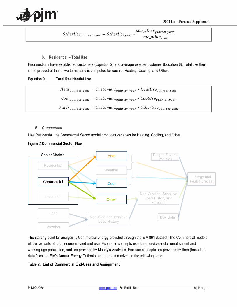
B. Commercial Like Residential, the Commercial Sector model produces variables for Heating, Cooling, and Other.

Figure 2. Commercial Sector Flow

The starting point for analysis is Commercial energy provided through the EIA 861 dataset. The Commercial models utilize two sets of data: economic and end-use. Economic concepts used are service sector employment and working-age population, and are provided by Moody’s Analytics. End-use concepts are provided by Itron (based on data from the EIA’s Annual Energy Outlook), and are summarized in the following table.

Table 2. List of Commercial End-Uses and Assignment




Bucket Use Type Definition

Heating Heating Heating

Cooling Cooling Cooling

Other Ventilation Ventilation

Other WtrHeat Water Heating

Other Cooking Cooking

Other Refrig Refrigeration

Other Lighting Lighting

Other Office Office Equipment (PCs)

Other Misc Miscellaneous

1. Commercial – Pre-process First we remove the year-to-year weather impacts to reveal Commercial demand’s underlying trend. Conceptually load growth can be decomposed into how much of the change is due to weather and how much is due to underlying trends (economics and utilization). Earlier attempts at Commercial did not include this step and the model was a single equation. While simple, this former method had difficulty separating how much of the trend was due to weather patterns versus underlying fundamentals. By pre-processing we seek to isolate the weather effect and identify the underlying fundamentals.

Equation 10. Extracting Weather Effect

𝑜𝑜𝑖𝑖𝑅𝑅𝑅𝑅_𝑐𝑐𝑛𝑛𝑐𝑐𝑐𝑐𝑔𝑔𝑦𝑦𝑦𝑦𝑦𝑦𝑦𝑦𝑦𝑦 =𝑐𝑐𝑛𝑛𝑐𝑐𝑐𝑐𝑔𝑔𝑦𝑦𝑦𝑦𝑦𝑦𝑦𝑦𝑦𝑦𝑐𝑐𝑛𝑛𝑐𝑐𝑐𝑐𝑔𝑔𝑦𝑦𝑦𝑦𝑦𝑦𝑦𝑦𝑦𝑦−1

= 𝐵𝐵0 + 𝐵𝐵1 ∗𝑐𝑐𝑐𝑐𝑐𝑐𝑜𝑜𝑦𝑦𝑦𝑦𝑦𝑦𝑦𝑦 ∗ 𝑐𝑐𝑜𝑜𝑜𝑜_𝑖𝑖𝑛𝑛𝑦𝑦𝑦𝑦𝑦𝑦𝑦𝑦

𝑐𝑐𝑐𝑐𝑐𝑐𝑜𝑜𝑦𝑦𝑦𝑦𝑦𝑦𝑦𝑦−1 ∗ 𝑐𝑐𝑜𝑜𝑜𝑜_𝑖𝑖𝑛𝑛𝑦𝑦𝑦𝑦𝑦𝑦𝑦𝑦−1+ 𝐵𝐵2 ∗

ℎ𝑐𝑐𝑒𝑒𝑐𝑐𝑦𝑦𝑦𝑦𝑦𝑦𝑦𝑦 ∗ ℎ𝑜𝑜𝑜𝑜_𝑖𝑖𝑛𝑛𝑦𝑦𝑦𝑦𝑦𝑦𝑦𝑦ℎ𝑐𝑐𝑒𝑒𝑐𝑐𝑦𝑦𝑦𝑦𝑦𝑦𝑦𝑦−1 ∗ ℎ𝑜𝑜𝑜𝑜_𝑖𝑖𝑛𝑛𝑦𝑦𝑦𝑦𝑦𝑦𝑦𝑦−1

cool and heat are end-use variables. Weather effect is then defined as

𝑃𝑃𝑐𝑐𝑐𝑐𝑜𝑜_𝑜𝑜𝑖𝑖𝑅𝑅𝑅𝑅_𝑤𝑤𝑐𝑐ℎ𝑐𝑐𝑦𝑦𝑦𝑦𝑦𝑦𝑦𝑦 = 𝐵𝐵1 ∗𝑐𝑐𝑐𝑐𝑐𝑐𝑜𝑜𝑦𝑦𝑦𝑦𝑦𝑦𝑦𝑦 ∗ 𝑐𝑐𝑜𝑜𝑜𝑜_𝑖𝑖𝑛𝑛𝑦𝑦𝑦𝑦𝑦𝑦𝑦𝑦

𝑐𝑐𝑐𝑐𝑐𝑐𝑜𝑜𝑦𝑦𝑦𝑦𝑦𝑦𝑦𝑦−1 ∗ 𝑐𝑐𝑜𝑜𝑜𝑜_𝑖𝑖𝑛𝑛𝑦𝑦𝑦𝑦𝑦𝑦𝑦𝑦−1+ 𝐵𝐵2 ∗

ℎ𝑐𝑐𝑒𝑒𝑐𝑐𝑦𝑦𝑦𝑦𝑦𝑦𝑦𝑦 ∗ ℎ𝑜𝑜𝑜𝑜_𝑖𝑖𝑛𝑛𝑦𝑦𝑦𝑦𝑦𝑦𝑦𝑦ℎ𝑐𝑐𝑒𝑒𝑐𝑐𝑦𝑦𝑦𝑦𝑦𝑦𝑦𝑦−1 ∗ ℎ𝑜𝑜𝑜𝑜_𝑖𝑖𝑛𝑛𝑦𝑦𝑦𝑦𝑦𝑦𝑦𝑦−1

The delta between energy growth and growth attributable to weather is growth attributable to underlying fundamentals. This will be referred to as pred_diff_left

𝑃𝑃𝑐𝑐𝑐𝑐𝑜𝑜_𝑜𝑜𝑖𝑖𝑅𝑅𝑅𝑅_𝑜𝑜𝑐𝑐𝑅𝑅𝑐𝑐𝑦𝑦𝑦𝑦𝑦𝑦𝑦𝑦 = 𝑜𝑜𝑖𝑖𝑅𝑅𝑅𝑅_𝑐𝑐𝑛𝑛𝑐𝑐𝑐𝑐𝑔𝑔𝑦𝑦𝑦𝑦𝑦𝑦𝑦𝑦𝑦𝑦 − 𝑃𝑃𝑐𝑐𝑐𝑐𝑜𝑜_𝑜𝑜𝑖𝑖𝑅𝑅𝑅𝑅_𝑤𝑤𝑐𝑐ℎ𝑐𝑐𝑦𝑦𝑦𝑦𝑦𝑦𝑦𝑦

pred_diff_left is a differenced time series, which needs to be converted into a non-differenced time series to be called left to be defined as follows

𝑜𝑜𝑐𝑐𝑅𝑅𝑐𝑐1998 = 1.0




For years after 1998

𝑜𝑜𝑐𝑐𝑅𝑅𝑐𝑐𝑦𝑦𝑦𝑦𝑦𝑦𝑦𝑦 = 𝑜𝑜𝑐𝑐𝑅𝑅𝑐𝑐𝑦𝑦𝑦𝑦𝑦𝑦𝑦𝑦−1 ∗ (1 + 𝑃𝑃𝑐𝑐𝑐𝑐𝑜𝑜_𝑜𝑜𝑖𝑖𝑅𝑅𝑅𝑅_𝑜𝑜𝑐𝑐𝑅𝑅𝑐𝑐𝑦𝑦𝑦𝑦𝑦𝑦𝑦𝑦)

2. Commercial – Drivers Drivers for commercial are working-age population, service sector employment, and end-use characteristics. Two potential drivers are defined d1 and d2.

Equation 11. Commercial Drivers

𝑜𝑜1𝑦𝑦𝑦𝑦𝑦𝑦𝑦𝑦 = 𝑃𝑃𝑐𝑐𝑃𝑃𝑐𝑐𝑜𝑜𝑒𝑒𝑐𝑐𝑖𝑖𝑐𝑐𝑛𝑛𝑦𝑦𝑦𝑦𝑦𝑦𝑦𝑦 ∗ 𝑐𝑐𝑛𝑛𝑜𝑜_𝑐𝑐𝑐𝑐𝑐𝑐𝑦𝑦𝑦𝑦𝑦𝑦𝑦𝑦

𝑜𝑜2𝑦𝑦𝑦𝑦𝑦𝑦𝑦𝑦 = 𝑐𝑐𝑐𝑐𝑐𝑐𝑠𝑠_𝑐𝑐𝑐𝑐𝑃𝑃𝑜𝑜𝑐𝑐𝑦𝑦𝑐𝑐𝑐𝑐𝑛𝑛𝑐𝑐𝑦𝑦𝑦𝑦𝑦𝑦𝑦𝑦 ∗ 𝑐𝑐𝑛𝑛𝑜𝑜_𝑐𝑐𝑐𝑐𝑐𝑐𝑦𝑦𝑦𝑦𝑦𝑦𝑦𝑦

where population is working-age population, serv_employment is service sector employment and end_use is the sum of all end-uses listed in Table 2

Correlation analysis of d1 and d2 with left is then run (defined in Equation 10). Final driver is a weighted combination of d1 and d2 based on this correlation. In the event that correlation calculations do not produce positive results, d1 and d2 are weighted evenly.

3. Commercial – Model Final model takes the driver variable and uses it in a model to forecast left. The fitted values of this formula are predicted values for Commercial energy.

Equation 12. Commercial Forecast Model

𝑜𝑜𝑐𝑐𝑅𝑅𝑐𝑐𝑦𝑦𝑦𝑦𝑦𝑦𝑦𝑦 = 𝐵𝐵0 + 𝐵𝐵1 ∗ 𝑐𝑐𝑐𝑐𝑐𝑐𝑛𝑛𝑜𝑜𝑦𝑦𝑦𝑦𝑦𝑦𝑦𝑦 + 𝐵𝐵2 ∗ 𝑜𝑜𝑐𝑐𝑖𝑖𝑠𝑠𝑐𝑐𝑐𝑐𝑦𝑦𝑦𝑦𝑦𝑦𝑦𝑦 + 𝐴𝐴𝐴𝐴(1)

where trend is a linear time trend

Fitted values from the model are appended to historical values (as defined in Equation 10). At this point, the Commercial demand series is in per-unitized form. Per-unit figures are thus multiplied by the corresponding Commercial energy figure from 1998. Assignments to Heat, Cool, and Other is then performed using the following formulas.

Equation 13. Assigning Commercial Demand to Heat, Cool, and Other

𝐻𝐻𝑐𝑐𝑒𝑒𝑐𝑐𝑦𝑦𝑦𝑦𝑦𝑦𝑦𝑦 = 𝐸𝐸𝑛𝑛𝑐𝑐𝑐𝑐𝑔𝑔𝑦𝑦𝑦𝑦𝑦𝑦𝑦𝑦𝑦𝑦 ∗ 𝐻𝐻𝑐𝑐𝑒𝑒𝑐𝑐𝑖𝑖𝑛𝑛𝑔𝑔_𝐸𝐸𝐻𝐻𝑦𝑦𝑦𝑦𝑦𝑦𝑦𝑦 𝑇𝑇𝑐𝑐𝑐𝑐𝑒𝑒𝑜𝑜_𝐸𝐸𝐻𝐻𝑦𝑦𝑦𝑦𝑦𝑦𝑦𝑦⁄

𝐶𝐶𝑐𝑐𝑐𝑐𝑜𝑜𝑦𝑦𝑦𝑦𝑦𝑦𝑦𝑦 = 𝐸𝐸𝑛𝑛𝑐𝑐𝑐𝑐𝑔𝑔𝑦𝑦𝑦𝑦𝑦𝑦𝑦𝑦𝑦𝑦 ∗ 𝐶𝐶𝑐𝑐𝑐𝑐𝑜𝑜𝑖𝑖𝑛𝑛𝑔𝑔_𝐸𝐸𝐻𝐻𝑦𝑦𝑦𝑦𝑦𝑦𝑦𝑦/𝑇𝑇𝑐𝑐𝑐𝑐𝑒𝑒𝑜𝑜_𝐸𝐸𝐻𝐻𝑦𝑦𝑦𝑦𝑦𝑦𝑦𝑦

𝑂𝑂𝑐𝑐ℎ𝑐𝑐𝑐𝑐𝑦𝑦𝑦𝑦𝑦𝑦𝑦𝑦 = 𝐸𝐸𝑛𝑛𝑐𝑐𝑐𝑐𝑔𝑔𝑦𝑦𝑦𝑦𝑦𝑦𝑦𝑦𝑦𝑦 ∗ 𝑂𝑂𝑐𝑐ℎ𝑐𝑐𝑐𝑐_𝐸𝐸𝐻𝐻𝑦𝑦𝑦𝑦𝑦𝑦𝑦𝑦/𝑇𝑇𝑐𝑐𝑐𝑐𝑒𝑒𝑜𝑜_𝐸𝐸𝐻𝐻𝑦𝑦𝑦𝑦𝑦𝑦𝑦𝑦

where Energy is total Commercial energy, Heating_EU, Cooling_EU, Other_EU, and Total_EU are from the end-use data as laid out in Table 2

Annual Heat, Cool, and Other series are converted to quarterly series using the intra-year path of the driver variable. It is composed of quarterly values relative to that year's annual average.




Equation 14. Quarterly Conversion of Heat, Cool, and Other

𝐻𝐻𝑐𝑐𝑒𝑒𝑐𝑐𝑞𝑞𝑞𝑞𝑦𝑦𝑦𝑦𝑞𝑞𝑦𝑦𝑦𝑦,𝑦𝑦𝑦𝑦𝑦𝑦𝑦𝑦 = 𝐻𝐻𝑐𝑐𝑒𝑒𝑐𝑐𝑦𝑦𝑦𝑦𝑦𝑦𝑦𝑦 ∗ 𝑜𝑜𝑐𝑐𝑖𝑖𝑠𝑠𝑐𝑐𝑐𝑐𝑞𝑞𝑞𝑞𝑦𝑦𝑦𝑦𝑞𝑞𝑦𝑦𝑦𝑦,𝑦𝑦𝑦𝑦𝑦𝑦𝑦𝑦/𝑜𝑜𝑐𝑐𝑖𝑖𝑠𝑠𝑐𝑐𝑐𝑐𝑦𝑦𝑦𝑦𝑦𝑦𝑦𝑦

𝐶𝐶𝑐𝑐𝑐𝑐𝑜𝑜𝑞𝑞𝑞𝑞𝑦𝑦𝑦𝑦𝑞𝑞𝑦𝑦𝑦𝑦,𝑦𝑦𝑦𝑦𝑦𝑦𝑦𝑦 = 𝐶𝐶𝑐𝑐𝑐𝑐𝑜𝑜𝑦𝑦𝑦𝑦𝑦𝑦𝑦𝑦 ∗ 𝑜𝑜𝑐𝑐𝑖𝑖𝑠𝑠𝑐𝑐𝑐𝑐𝑞𝑞𝑞𝑞𝑦𝑦𝑦𝑦𝑞𝑞𝑦𝑦𝑦𝑦,𝑦𝑦𝑦𝑦𝑦𝑦𝑦𝑦/𝑜𝑜𝑐𝑐𝑖𝑖𝑠𝑠𝑐𝑐𝑐𝑐𝑦𝑦𝑦𝑦𝑦𝑦𝑦𝑦

𝑂𝑂𝑐𝑐ℎ𝑐𝑐𝑐𝑐𝑞𝑞𝑞𝑞𝑦𝑦𝑦𝑦𝑞𝑞𝑦𝑦𝑦𝑦,𝑦𝑦𝑦𝑦𝑦𝑦𝑦𝑦 = 𝑂𝑂𝑐𝑐ℎ𝑐𝑐𝑐𝑐𝑦𝑦𝑦𝑦𝑦𝑦𝑦𝑦 ∗ 𝑜𝑜𝑐𝑐𝑖𝑖𝑠𝑠𝑐𝑐𝑐𝑐𝑞𝑞𝑞𝑞𝑦𝑦𝑦𝑦𝑞𝑞𝑦𝑦𝑦𝑦,𝑦𝑦𝑦𝑦𝑦𝑦𝑦𝑦/𝑜𝑜𝑐𝑐𝑖𝑖𝑠𝑠𝑐𝑐𝑐𝑐𝑦𝑦𝑦𝑦𝑦𝑦𝑦𝑦

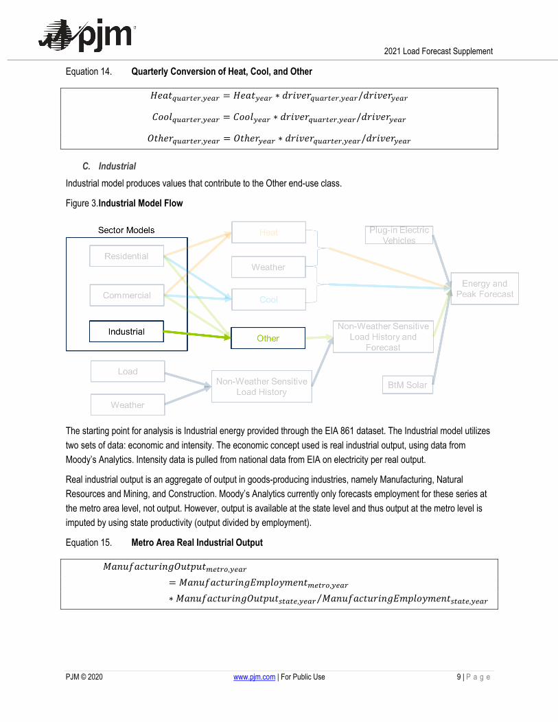
C. Industrial Industrial model produces values that contribute to the Other end-use class.

Figure 3. Industrial Model Flow

The starting point for analysis is Industrial energy provided through the EIA 861 dataset. The Industrial model utilizes two sets of data: economic and intensity. The economic concept used is real industrial output, using data from Moody’s Analytics. Intensity data is pulled from national data from EIA on electricity per real output.

Real industrial output is an aggregate of output in goods-producing industries, namely Manufacturing, Natural Resources and Mining, and Construction. Moody’s Analytics currently only forecasts employment for these series at the metro area level, not output. However, output is available at the state level and thus output at the metro level is imputed by using state productivity (output divided by employment).

Equation 15. Metro Area Real Industrial Output

𝑀𝑀𝑒𝑒𝑛𝑛𝑐𝑐𝑅𝑅𝑒𝑒𝑐𝑐𝑐𝑐𝑐𝑐𝑐𝑐𝑖𝑖𝑛𝑛𝑔𝑔𝑂𝑂𝑐𝑐𝑐𝑐𝑃𝑃𝑐𝑐𝑐𝑐𝑚𝑚𝑦𝑦𝑞𝑞𝑦𝑦𝑚𝑚,𝑦𝑦𝑦𝑦𝑦𝑦𝑦𝑦

= 𝑀𝑀𝑒𝑒𝑛𝑛𝑐𝑐𝑅𝑅𝑒𝑒𝑐𝑐𝑐𝑐𝑐𝑐𝑐𝑐𝑖𝑖𝑛𝑛𝑔𝑔𝐸𝐸𝑐𝑐𝑃𝑃𝑜𝑜𝑐𝑐𝑦𝑦𝑐𝑐𝑐𝑐𝑛𝑛𝑐𝑐𝑚𝑚𝑦𝑦𝑞𝑞𝑦𝑦𝑚𝑚,𝑦𝑦𝑦𝑦𝑦𝑦𝑦𝑦

∗ 𝑀𝑀𝑒𝑒𝑛𝑛𝑐𝑐𝑅𝑅𝑒𝑒𝑐𝑐𝑐𝑐𝑐𝑐𝑐𝑐𝑖𝑖𝑛𝑛𝑔𝑔𝑂𝑂𝑐𝑐𝑐𝑐𝑃𝑃𝑐𝑐𝑐𝑐𝑠𝑠𝑞𝑞𝑦𝑦𝑞𝑞𝑦𝑦,𝑦𝑦𝑦𝑦𝑦𝑦𝑦𝑦 𝑀𝑀𝑒𝑒𝑛𝑛𝑐𝑐𝑅𝑅𝑒𝑒𝑐𝑐𝑐𝑐𝑐𝑐𝑐𝑐𝑖𝑖𝑛𝑛𝑔𝑔𝐸𝐸𝑐𝑐𝑃𝑃𝑜𝑜𝑐𝑐𝑦𝑦𝑐𝑐𝑐𝑐𝑛𝑛𝑐𝑐𝑠𝑠𝑞𝑞𝑦𝑦𝑞𝑞𝑦𝑦,𝑦𝑦𝑦𝑦𝑦𝑦𝑦𝑦⁄




𝑀𝑀𝑖𝑖𝑛𝑛𝑖𝑖𝑛𝑛𝑔𝑔𝑂𝑂𝑐𝑐𝑐𝑐𝑃𝑃𝑐𝑐𝑐𝑐𝑚𝑚𝑦𝑦𝑞𝑞𝑦𝑦𝑚𝑚,𝑦𝑦𝑦𝑦𝑦𝑦𝑦𝑦

= 𝑀𝑀𝑖𝑖𝑛𝑛𝑖𝑖𝑛𝑛𝑔𝑔𝐸𝐸𝑐𝑐𝑃𝑃𝑜𝑜𝑐𝑐𝑦𝑦𝑐𝑐𝑐𝑐𝑛𝑛𝑐𝑐𝑚𝑚𝑦𝑦𝑞𝑞𝑦𝑦𝑚𝑚,𝑦𝑦𝑦𝑦𝑦𝑦𝑦𝑦

∗ 𝑀𝑀𝑖𝑖𝑛𝑛𝑖𝑖𝑛𝑛𝑔𝑔𝑂𝑂𝑐𝑐𝑐𝑐𝑃𝑃𝑐𝑐𝑐𝑐𝑠𝑠𝑞𝑞𝑦𝑦𝑞𝑞𝑦𝑦,𝑦𝑦𝑦𝑦𝑦𝑦𝑦𝑦 𝑀𝑀𝑖𝑖𝑛𝑛𝑖𝑖𝑛𝑛𝑔𝑔𝐸𝐸𝑐𝑐𝑃𝑃𝑜𝑜𝑐𝑐𝑦𝑦𝑐𝑐𝑐𝑐𝑛𝑛𝑐𝑐𝑠𝑠𝑞𝑞𝑦𝑦𝑞𝑞𝑦𝑦,𝑦𝑦𝑦𝑦𝑦𝑦𝑦𝑦⁄

𝐶𝐶𝑐𝑐𝑛𝑛𝑐𝑐𝑐𝑐𝑐𝑐𝑐𝑐𝑐𝑐𝑐𝑐𝑖𝑖𝑐𝑐𝑛𝑛𝑂𝑂𝑐𝑐𝑐𝑐𝑃𝑃𝑐𝑐𝑐𝑐𝑚𝑚𝑦𝑦𝑞𝑞𝑦𝑦𝑚𝑚,𝑦𝑦𝑦𝑦𝑦𝑦𝑦𝑦

= 𝐶𝐶𝑐𝑐𝑛𝑛𝑐𝑐𝑐𝑐𝑐𝑐𝑐𝑐𝑐𝑐𝑐𝑐𝑖𝑖𝑐𝑐𝑛𝑛𝐸𝐸𝑐𝑐𝑃𝑃𝑜𝑜𝑐𝑐𝑦𝑦𝑐𝑐𝑐𝑐𝑛𝑛𝑐𝑐𝑚𝑚𝑦𝑦𝑞𝑞𝑦𝑦𝑚𝑚,𝑦𝑦𝑦𝑦𝑦𝑦𝑦𝑦

∗ 𝐶𝐶𝑐𝑐𝑛𝑛𝑐𝑐𝑐𝑐𝑐𝑐𝑐𝑐𝑐𝑐𝑐𝑐𝑖𝑖𝑐𝑐𝑛𝑛𝑂𝑂𝑐𝑐𝑐𝑐𝑃𝑃𝑐𝑐𝑐𝑐𝑠𝑠𝑞𝑞𝑦𝑦𝑞𝑞𝑦𝑦,𝑦𝑦𝑦𝑦𝑦𝑦𝑦𝑦 𝐶𝐶𝑐𝑐𝑛𝑛𝑐𝑐𝑐𝑐𝑐𝑐𝑐𝑐𝑐𝑐𝑐𝑐𝑖𝑖𝑐𝑐𝑛𝑛𝐸𝐸𝑐𝑐𝑃𝑃𝑜𝑜𝑐𝑐𝑦𝑦𝑐𝑐𝑐𝑐𝑛𝑛𝑐𝑐𝑠𝑠𝑞𝑞𝑦𝑦𝑞𝑞𝑦𝑦,𝑦𝑦𝑦𝑦𝑦𝑦𝑦𝑦⁄

𝑂𝑂𝑐𝑐𝑐𝑐𝑃𝑃𝑐𝑐𝑐𝑐𝑚𝑚𝑦𝑦𝑞𝑞𝑦𝑦𝑚𝑚,𝑦𝑦𝑦𝑦𝑦𝑦𝑦𝑦

= 𝑀𝑀𝑒𝑒𝑛𝑛𝑐𝑐𝑅𝑅𝑒𝑒𝑐𝑐𝑐𝑐𝑐𝑐𝑐𝑐𝑖𝑖𝑛𝑛𝑔𝑔𝑂𝑂𝑐𝑐𝑐𝑐𝑃𝑃𝑐𝑐𝑐𝑐𝑚𝑚𝑦𝑦𝑞𝑞𝑦𝑦𝑚𝑚,𝑦𝑦𝑦𝑦𝑦𝑦𝑦𝑦 + 𝑀𝑀𝑖𝑖𝑛𝑛𝑖𝑖𝑛𝑛𝑔𝑔𝑂𝑂𝑐𝑐𝑐𝑐𝑃𝑃𝑐𝑐𝑐𝑐𝑚𝑚𝑦𝑦𝑞𝑞𝑦𝑦𝑚𝑚,𝑦𝑦𝑦𝑦𝑦𝑦𝑦𝑦

+ 𝐶𝐶𝑐𝑐𝑛𝑛𝑐𝑐𝑐𝑐𝑐𝑐𝑐𝑐𝑐𝑐𝑐𝑐𝑖𝑖𝑐𝑐𝑛𝑛𝑂𝑂𝑐𝑐𝑐𝑐𝑃𝑃𝑐𝑐𝑐𝑐𝑚𝑚𝑦𝑦𝑞𝑞𝑦𝑦𝑚𝑚,𝑦𝑦𝑦𝑦𝑦𝑦𝑦𝑦

where metro areas are assigned to states based on location

Industrial intensity is defined as industrial energy use per real output. The concept is based on national data. History considers Industrial Electricity Sales1 from the EIA divided by Industrial Output from Moody’s Analytics, and the forecast is from the EIA’s Annual Energy Outlook2.

Economics and intensity are multiplied together to provide the industrial driver variable (referred to below as use) that is then used in the Industrial Sector model. Fitted values from this model are then appended to historical values.

Equation 16. Industrial Forecast Model and Quarterly Conversion

𝑐𝑐𝑛𝑛𝑐𝑐𝑐𝑐𝑔𝑔𝑦𝑦𝑦𝑦𝑦𝑦𝑦𝑦𝑦𝑦 = 𝐵𝐵1 ∗ 𝑐𝑐𝑐𝑐𝑐𝑐𝑦𝑦𝑦𝑦𝑦𝑦𝑦𝑦 + 𝐴𝐴𝐴𝐴(1)

Annual values are then converted to quarterly using the intra-year path of the driver variable. It is composed of quarterly values relative to that year's annual average.

𝑐𝑐𝑛𝑛𝑐𝑐𝑐𝑐𝑔𝑔𝑦𝑦𝑞𝑞𝑞𝑞𝑦𝑦𝑦𝑦𝑞𝑞𝑦𝑦𝑦𝑦,𝑦𝑦𝑦𝑦𝑦𝑦𝑦𝑦 = 𝑐𝑐𝑛𝑛𝑐𝑐𝑐𝑐𝑔𝑔𝑦𝑦𝑦𝑦𝑦𝑦𝑦𝑦𝑦𝑦 ∗ 𝑐𝑐𝑐𝑐𝑐𝑐𝑞𝑞𝑞𝑞𝑦𝑦𝑦𝑦𝑞𝑞𝑦𝑦𝑦𝑦,𝑦𝑦𝑦𝑦𝑦𝑦𝑦𝑦/𝑐𝑐𝑐𝑐𝑐𝑐𝑦𝑦𝑦𝑦𝑦𝑦𝑦𝑦

D. Use Indexes At this point, developing the Heat, Cool, and Other Use Indexes is straightforward as each is the sum of the relevant sector variables developed. This is summarized in the below formulas.

Equation 17. Use Indexes

𝐻𝐻𝑐𝑐𝑒𝑒𝑐𝑐𝑞𝑞𝑞𝑞𝑦𝑦𝑦𝑦𝑞𝑞𝑦𝑦𝑦𝑦,𝑦𝑦𝑦𝑦𝑦𝑦𝑦𝑦 = 𝐴𝐴𝑐𝑐𝑐𝑐𝑖𝑖𝑜𝑜𝑐𝑐𝑛𝑛𝑐𝑐𝑖𝑖𝑒𝑒𝑜𝑜_𝐻𝐻𝑐𝑐𝑒𝑒𝑐𝑐𝑖𝑖𝑛𝑛𝑔𝑔𝑞𝑞𝑞𝑞𝑦𝑦𝑦𝑦𝑞𝑞𝑦𝑦𝑦𝑦,𝑦𝑦𝑦𝑦𝑦𝑦𝑦𝑦 + 𝐶𝐶𝑐𝑐𝑐𝑐𝑐𝑐𝑐𝑐𝑐𝑐𝑐𝑐𝑖𝑖𝑒𝑒𝑜𝑜_𝐻𝐻𝑐𝑐𝑒𝑒𝑐𝑐𝑖𝑖𝑛𝑛𝑔𝑔𝑞𝑞𝑞𝑞𝑦𝑦𝑦𝑦𝑞𝑞𝑦𝑦𝑦𝑦,𝑦𝑦𝑦𝑦𝑦𝑦𝑦𝑦

1 History compiled using EIA’s Electric Power Monthly Table 5.1 (https://www.eia.gov/electricity/monthly/) and the EIA table

Retail Sales of Electricity by State by Sector by Provider (https://www.eia.gov/electricity/data/state/). 2 Forecast comes from the EIA’s Annual Energy Outlook, the Industrial Table

(https://www.eia.gov/outlooks/aeo/data/browser/#/?id=6-AEO2020&cases=ref2020&sourcekey=0). Concept is Energy Consumption per dollar of Shipments (thousand Btu per 2009 dollar) - Purchased Electricity


https://www.eia.gov/electricity/monthly/

https://www.eia.gov/electricity/data/state/

https://www.eia.gov/outlooks/aeo/data/browser/#/?id=6-AEO2020&cases=ref2020&sourcekey=0



𝐶𝐶𝑐𝑐𝑐𝑐𝑜𝑜𝑞𝑞𝑞𝑞𝑦𝑦𝑦𝑦𝑞𝑞𝑦𝑦𝑦𝑦,𝑦𝑦𝑦𝑦𝑦𝑦𝑦𝑦 = 𝐴𝐴𝑐𝑐𝑐𝑐𝑖𝑖𝑜𝑜𝑐𝑐𝑛𝑛𝑐𝑐𝑖𝑖𝑒𝑒𝑜𝑜_𝐶𝐶𝑐𝑐𝑐𝑐𝑜𝑜𝑖𝑖𝑛𝑛𝑔𝑔𝑞𝑞𝑞𝑞𝑦𝑦𝑦𝑦𝑞𝑞𝑦𝑦𝑦𝑦,𝑦𝑦𝑦𝑦𝑦𝑦𝑦𝑦 + 𝐶𝐶𝑐𝑐𝑐𝑐𝑐𝑐𝑐𝑐𝑐𝑐𝑐𝑐𝑖𝑖𝑒𝑒𝑜𝑜_𝐶𝐶𝑐𝑐𝑐𝑐𝑜𝑜𝑖𝑖𝑛𝑛𝑔𝑔𝑞𝑞𝑞𝑞𝑦𝑦𝑦𝑦𝑞𝑞𝑦𝑦𝑦𝑦,𝑦𝑦𝑦𝑦𝑦𝑦𝑦𝑦

𝑂𝑂𝑐𝑐ℎ𝑐𝑐𝑐𝑐𝑞𝑞𝑞𝑞𝑦𝑦𝑦𝑦𝑞𝑞𝑦𝑦𝑦𝑦,𝑦𝑦𝑦𝑦𝑦𝑦𝑦𝑦 = 𝐴𝐴𝑐𝑐𝑐𝑐𝑖𝑖𝑜𝑜𝑐𝑐𝑛𝑛𝑐𝑐𝑖𝑖𝑒𝑒𝑜𝑜_𝑂𝑂𝑐𝑐ℎ𝑐𝑐𝑐𝑐𝑞𝑞𝑞𝑞𝑦𝑦𝑦𝑦𝑞𝑞𝑦𝑦𝑦𝑦,𝑦𝑦𝑦𝑦𝑦𝑦𝑦𝑦 + 𝐶𝐶𝑐𝑐𝑐𝑐𝑐𝑐𝑐𝑐𝑐𝑐𝑐𝑐𝑖𝑖𝑒𝑒𝑜𝑜_𝑂𝑂𝑐𝑐ℎ𝑐𝑐𝑐𝑐𝑞𝑞𝑞𝑞𝑦𝑦𝑦𝑦𝑞𝑞𝑦𝑦𝑦𝑦,𝑦𝑦𝑦𝑦𝑦𝑦𝑦𝑦 +𝐼𝐼𝑛𝑛𝑜𝑜𝑐𝑐𝑐𝑐𝑐𝑐𝑐𝑐𝑖𝑖𝑒𝑒𝑜𝑜𝑞𝑞𝑞𝑞𝑦𝑦𝑦𝑦𝑞𝑞𝑦𝑦𝑦𝑦,𝑦𝑦𝑦𝑦𝑦𝑦𝑦𝑦

III. Non-Weather Sensitive Load Non-weather sensitive load is what load would have been absent the impacts of Cooling and Heating equipment. It is not an observed concept, but rather something estimated through the use of models. The idea behind using non-weather sensitive load is that taking this step allows the model to better align the type of load with its appropriate drivers. In other words, this seeks to limit the impact of the Other End-Use index on the model’s weather response, or the impact of the Cooling End-Use index on non-weather sensitive load.

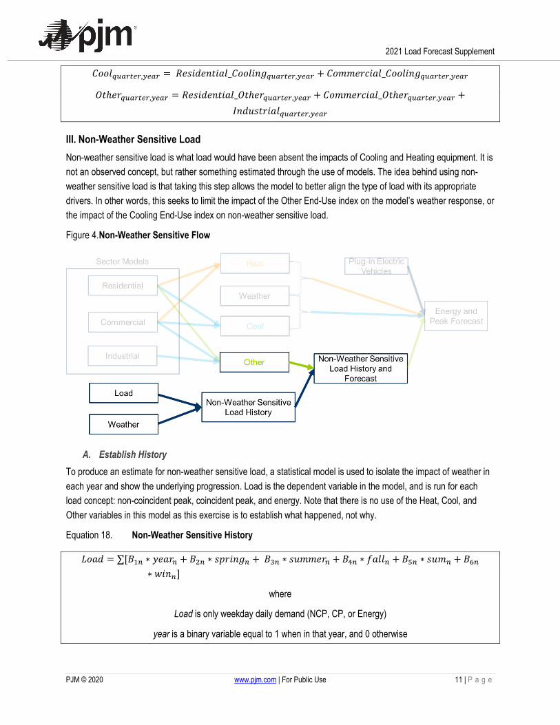
Figure 4. Non-Weather Sensitive Flow

A. Establish History To produce an estimate for non-weather sensitive load, a statistical model is used to isolate the impact of weather in each year and show the underlying progression. Load is the dependent variable in the model, and is run for each load concept: non-coincident peak, coincident peak, and energy. Note that there is no use of the Heat, Cool, and Other variables in this model as this exercise is to establish what happened, not why.

Equation 18. Non-Weather Sensitive History

𝐿𝐿𝑐𝑐𝑒𝑒𝑜𝑜 = ∑[𝐵𝐵1𝑛𝑛 ∗ 𝑦𝑦𝑐𝑐𝑒𝑒𝑐𝑐𝑛𝑛 + 𝐵𝐵2𝑛𝑛 ∗ 𝑐𝑐𝑃𝑃𝑐𝑐𝑖𝑖𝑛𝑛𝑔𝑔𝑛𝑛 + 𝐵𝐵3𝑛𝑛 ∗ 𝑐𝑐𝑐𝑐𝑐𝑐𝑐𝑐𝑐𝑐𝑐𝑐𝑛𝑛 + 𝐵𝐵4𝑛𝑛 ∗ 𝑅𝑅𝑒𝑒𝑜𝑜𝑜𝑜𝑛𝑛 + 𝐵𝐵5𝑛𝑛 ∗ 𝑐𝑐𝑐𝑐𝑐𝑐𝑛𝑛 + 𝐵𝐵6𝑛𝑛∗ 𝑤𝑤𝑖𝑖𝑛𝑛𝑛𝑛]

where

Load is only weekday daily demand (NCP, CP, or Energy)

year is a binary variable equal to 1 when in that year, and 0 otherwise




n is a year from 1998 to 2020

spring, summer, and fall are binary variables equal to 1 when in that season of that year, and 0 otherwise

sum and win are summer and winter weather variables, described in a later section

To determine non-weather sensitive history, the sum and win terms are removed

𝑁𝑁𝑐𝑐𝑛𝑛 −𝐸𝐸𝑐𝑐𝑒𝑒𝑐𝑐ℎ𝑐𝑐𝑐𝑐 𝑆𝑆𝑐𝑐𝑛𝑛𝑐𝑐𝑖𝑖𝑐𝑐𝑖𝑖𝑠𝑠𝑐𝑐 𝐿𝐿𝑐𝑐𝑒𝑒𝑜𝑜𝑠𝑠𝑦𝑦𝑦𝑦𝑠𝑠𝑚𝑚𝑛𝑛,𝑦𝑦𝑦𝑦𝑦𝑦𝑦𝑦

= ∑[𝐵𝐵1𝑛𝑛 ∗ 𝑦𝑦𝑐𝑐𝑒𝑒𝑐𝑐𝑛𝑛 + 𝐵𝐵2𝑛𝑛 ∗ 𝑐𝑐𝑃𝑃𝑐𝑐𝑖𝑖𝑛𝑛𝑔𝑔𝑛𝑛 + 𝐵𝐵3𝑛𝑛 ∗ 𝑐𝑐𝑐𝑐𝑐𝑐𝑐𝑐𝑐𝑐𝑐𝑐𝑛𝑛 + 𝐵𝐵4𝑛𝑛 ∗ 𝑅𝑅𝑒𝑒𝑜𝑜𝑜𝑜𝑛𝑛]

B. Establish Forecast Non-weather sensitive history is then used as a dependent variable in a model to derive a forecast. The Other Use index previously determined is used as the primary driver.

Equation 19. Non-Weather Sensitive Forecast

𝑁𝑁𝑐𝑐𝑛𝑛 −𝐸𝐸𝑐𝑐𝑒𝑒𝑐𝑐ℎ𝑐𝑐𝑐𝑐 𝑆𝑆𝑐𝑐𝑛𝑛𝑐𝑐𝑖𝑖𝑐𝑐𝑖𝑖𝑠𝑠𝑐𝑐 𝐿𝐿𝑐𝑐𝑒𝑒𝑜𝑜𝑠𝑠𝑦𝑦𝑦𝑦𝑠𝑠𝑚𝑚𝑛𝑛,𝑦𝑦𝑦𝑦𝑦𝑦𝑦𝑦

= 𝐵𝐵0 + 𝐵𝐵1 ∗ 𝑐𝑐𝑐𝑐𝑐𝑐𝑛𝑛𝑜𝑜 + 𝐵𝐵2 ∗ 𝑂𝑂𝑐𝑐ℎ𝑐𝑐𝑐𝑐 + 𝐵𝐵3 ∗ 𝑐𝑐𝑐𝑐𝑐𝑐𝑐𝑐𝑐𝑐𝑐𝑐_𝑐𝑐𝑐𝑐ℎ𝑐𝑐𝑐𝑐 + 𝐵𝐵4 ∗ 𝑅𝑅𝑒𝑒𝑜𝑜𝑜𝑜_𝑐𝑐𝑐𝑐ℎ𝑐𝑐𝑐𝑐 + 𝐵𝐵5∗ 𝑐𝑐𝑃𝑃𝑐𝑐𝑖𝑖𝑛𝑛𝑔𝑔_𝑐𝑐𝑐𝑐ℎ𝑐𝑐𝑐𝑐 + 𝐴𝐴𝐴𝐴(1) + 𝐴𝐴𝐴𝐴(4)

Where Non-Weather Sensitive Load is according to the model under study (NCP, CP, Energy)

trend is a linear time trend

Other is the Other Use index

summer_other, fall_other, and spring_other are Other interacted with seasonal binaries

AR(1) and AR(4) are autoregressive error terms for the prior period and the prior season, respectively

The fitted results of the model become the forecast portion of the time series, with the history having previously been established in Equation 1.

IV. Weather Variables Weather variables are defined at the zone level. Zonal weather is a weighted average of weather stations, defined below3.

Table 3. Weather Station Assignment

Zone Weather Station Weight

Zone Weather Station Weight

AE ACY 100.0%

JCPL ACY 25.0%

AEP CAK 15.1%

JCPL EWR 75.0%

AEP CMH 23.4%

METED ABE 50.0%

3 Weather station weights are provided by Electric Distribution Companies (EDCs).




AEP CRW 22.6%

METED PHL 50.0%

AEP FWA 22.7%

PECO PHL 100.0%

AEP ROA 16.2%

PENLC ERI 50.0%

APS IAD 30.0%

PENLC IPT 50.0%

APS PIT 70.0%

PEPCO DCA 100.0%

ATSI CAK 46.5%

PL ABE 25.0%

ATSI CLE 30.0%

PL AVP 25.0%

ATSI PIT 8.5%

PL IPT 25.0%

ATSI TOL 15.0%

PL MDT 25.0%

BGE BWI 100.0%

PS EWR 100.0%

COMED ORD 100.0%

RECO EWR 100.0%

DAYTON DAY 100.0%

UGI AVP 100.0%

DPL ILG 70.0%

VEPCO IAD 33.3%

DPL WAL 30.0%

VEPCO ORF 33.3%

DQE PIT 100.0%

VEPCO RIC 33.3%

DUKE CVG 100.0%

EKPC CVG 25.0%

EKPC LEX 49.0%

EKPC SDF 26.0%

A. Heating and Cooling PJM uses different variables for cooling periods and heating periods to capture the impact of weather on load across seasons. The cooling period uses Cooling Degree Days (CDD), Lagged Cooling Degree Days, and maximum daily Temperature Humidity Index (THI), laid out in Equation 1. The heating period uses a three-hour moving average of the Winter Weather Parameter (WWP) at the time of the peak, average daily WWP, Lagged average daily WWP, and minimum daily WWP, laid out in Equation 2.

Equation 20. Cooling Period Weather Variables

Cooling Degree Days (CDD)

𝐶𝐶𝐷𝐷𝐷𝐷 = max (𝑒𝑒𝑠𝑠𝑔𝑔_𝑐𝑐𝑐𝑐𝑐𝑐𝑃𝑃 − 65 , 0)

where avg_temp is average daily temperature




Temperature Humidity Index (THI)

If temp >= 58 then

𝑇𝑇𝐻𝐻𝐼𝐼 = 𝑐𝑐𝑐𝑐𝑐𝑐𝑃𝑃 − 0.55 ∗ (1 − ℎ𝑐𝑐𝑐𝑐𝑖𝑖𝑜𝑜𝑖𝑖𝑐𝑐𝑦𝑦) ∗ (𝑐𝑐𝑐𝑐𝑐𝑐𝑃𝑃 − 58)

Else

𝑇𝑇𝐻𝐻𝐼𝐼 = 𝑐𝑐𝑐𝑐𝑐𝑐𝑃𝑃

where temp is temperature

humidity is relative humidity (100% = 1.0)

Equation 21. Heating Period Weather Variables

Wind-Adjusted Temperature (WWP)

If wind > 10

𝐸𝐸𝐸𝐸𝐻𝐻 = 𝑐𝑐𝑐𝑐𝑐𝑐𝑃𝑃 − 0.5 ∗ (𝑤𝑤𝑖𝑖𝑛𝑛𝑜𝑜 − 10)

Else

𝐸𝐸𝐸𝐸𝐻𝐻 = 𝑐𝑐𝑐𝑐𝑐𝑐𝑃𝑃

where temp is temperature

wind is wind speed (MPH)

Weather concepts are then normalized such that they can be later combined.

Equation 22. Normalize Weather Variables

For each weather concept

𝐸𝐸𝑐𝑐ℎ𝑐𝑐_𝑁𝑁𝑐𝑐𝑐𝑐𝑐𝑐𝑑𝑑𝑦𝑦𝑑𝑑𝑑𝑑𝑦𝑦 = (𝐸𝐸𝑐𝑐ℎ𝑐𝑐𝑑𝑑𝑦𝑦𝑑𝑑𝑑𝑑𝑦𝑦 − 𝑀𝑀𝑐𝑐𝑒𝑒𝑛𝑛_𝐸𝐸𝑐𝑐ℎ𝑐𝑐)/ (𝑆𝑆𝑐𝑐𝑜𝑜_𝐷𝐷𝑐𝑐𝑠𝑠_𝐸𝐸𝑐𝑐ℎ𝑐𝑐)

where means and standard deviations are computed over history for months May through September for cooling variables and January, February, and December for heating variables

Seasonal regression models are then run on load for each weather variable. The Sum of Squared Errors (SSE) is saved and then the reciprocals are used as weights (i.e., the less the error, the higher the weight). The end result is a single weather variable that is a weighted composite.

Equation 23. Developing Weights for Weather Variables

𝐿𝐿𝑐𝑐𝑒𝑒𝑜𝑜 = ∑[𝐵𝐵1𝑛𝑛 ∗ 𝑦𝑦𝑐𝑐𝑒𝑒𝑐𝑐𝑛𝑛] + 𝑤𝑤𝑐𝑐ℎ𝑐𝑐

Load is according to the model under study (NCP, CP, Energy) with weekends and holidays removed

year is a binary variable equal to 1 when in that year, and 0 otherwise

n is a year from 1998 to 2020




wthr is the weather concept

For each weather concept i, the reciprocal of Sum of Squared Errors (SSE) is stored, (1/SSEi)

First, calculate the total for each season s (heating or cooling)

𝑇𝑇𝑐𝑐𝑐𝑐𝑒𝑒𝑜𝑜𝑠𝑠 = ∑(1/𝑆𝑆𝑆𝑆𝐸𝐸𝑑𝑑)

And then calculate weighti. Weights are calculated for each model type (NCP, CP, Energy)

𝑤𝑤𝑐𝑐𝑖𝑖𝑔𝑔ℎ𝑐𝑐𝑑𝑑,𝑠𝑠 = (1/𝑆𝑆𝑆𝑆𝐸𝐸𝑑𝑑)/𝑇𝑇𝑐𝑐𝑐𝑐𝑒𝑒𝑜𝑜𝑠𝑠

Weather variables are then combined with their respective weights and summed to produce a composite weather variable for each season.

Equation 24. Composite Weather Variables

𝑐𝑐𝑐𝑐𝑐𝑐_𝑠𝑠𝑒𝑒𝑐𝑐 = ∑(𝑤𝑤𝑐𝑐𝑖𝑖𝑔𝑔ℎ𝑐𝑐𝑑𝑑 ∗ 𝑤𝑤𝑐𝑐ℎ𝑐𝑐𝑑𝑑)

where weather concepts included are Cooling Degree Days (CDD), Lagged Cooling Degree Days, and maximum daily Temperature Humidity Index (THI)

𝑤𝑤𝑖𝑖𝑛𝑛_𝑠𝑠𝑒𝑒𝑐𝑐 = ∑(𝑤𝑤𝑐𝑐𝑖𝑖𝑔𝑔ℎ𝑐𝑐𝑑𝑑 ∗ 𝑤𝑤𝑐𝑐ℎ𝑐𝑐𝑑𝑑)

where weather concepts included are three-hour moving average of the Winter Weather Parameter (WWP) at the time of the peak, average daily WWP, Lagged average daily WWP, and minimum daily WWP

Once sum_var and win_var are constructed, each series is shifted such that sum_var has a minimum value of 0 and win_var has a maximum value of 0.

B. Cloud Cover Cloud cover is also included in the model to help capture the weather effects outside temperature and wind speed. Increased cloud cover in cooling periods could potentially reduce load, and conversely increase load in heating periods. Cloud cover is reported on a scale of 0 to 8, with higher values reflecting increased cloud cover.

Equation 25. Cloud Cover Variables

For Cooling Period

Afternoon cloud cover: aftercloud is average of cloud cover over Hour Ending 13 through 18

Evening cloud cover: evencloud is average of cloud cover over Hour Ending 19 through 24

For Heating Period

Morning cloud cover: morncloud is average of cloud cover over Hour Ending 7 through 12

Evening cloud cover: evencloud is average of cloud cover over Hour Ending 19 through 24




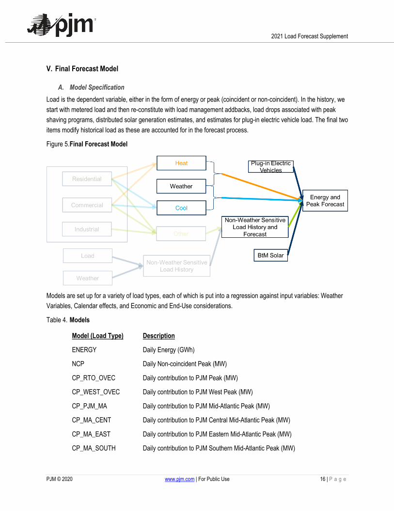
V. Final Forecast Model

A. Model Specification Load is the dependent variable, either in the form of energy or peak (coincident or non-coincident). In the history, we start with metered load and then re-constitute with load management addbacks, load drops associated with peak shaving programs, distributed solar generation estimates, and estimates for plug-in electric vehicle load. The final two items modify historical load as these are accounted for in the forecast process.

Figure 5. Final Forecast Model

Models are set up for a variety of load types, each of which is put into a regression against input variables: Weather Variables, Calendar effects, and Economic and End-Use considerations.

Table 4. Models

Model (Load Type) Description

ENERGY Daily Energy (GWh)

NCP Daily Non-coincident Peak (MW)

CP_RTO_OVEC Daily contribution to PJM Peak (MW)

CP_WEST_OVEC Daily contribution to PJM West Peak (MW)

CP_PJM_MA Daily contribution to PJM Mid-Atlantic Peak (MW)

CP_MA_CENT Daily contribution to PJM Central Mid-Atlantic Peak (MW)

CP_MA_EAST Daily contribution to PJM Eastern Mid-Atlantic Peak (MW)

CP_MA_SOUTH Daily contribution to PJM Southern Mid-Atlantic Peak (MW)




CP_MA_WEST Daily contribution to PJM Western Mid-Atlantic Peak (MW)

CP_GPU Daily contribution to FE-East Peak (MW)

CP_PLGRP Daily contribution to PLGRP Peak (MW)

Each regression model has the same set-up.

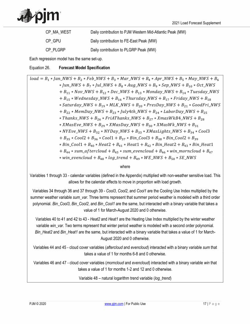
Equation 26. Forecast Model Specification

𝑜𝑜𝑐𝑐𝑒𝑒𝑜𝑜 = 𝐵𝐵1 ∗ 𝐽𝐽𝑒𝑒𝑛𝑛_𝑁𝑁𝐸𝐸𝑆𝑆 + 𝐵𝐵2 ∗ 𝐸𝐸𝑐𝑐𝐹𝐹_𝑁𝑁𝐸𝐸𝑆𝑆 + 𝐵𝐵3 ∗ 𝑀𝑀𝑒𝑒𝑐𝑐_𝑁𝑁𝐸𝐸𝑆𝑆 + 𝐵𝐵4 ∗ 𝐴𝐴𝑃𝑃𝑐𝑐_𝑁𝑁𝐸𝐸𝑆𝑆 + 𝐵𝐵5 ∗ 𝑀𝑀𝑒𝑒𝑦𝑦_𝑁𝑁𝐸𝐸𝑆𝑆 + 𝐵𝐵6∗ 𝐽𝐽𝑐𝑐𝑛𝑛_𝑁𝑁𝐸𝐸𝑆𝑆 + 𝐵𝐵7 ∗ 𝐽𝐽𝑐𝑐𝑜𝑜_𝑁𝑁𝐸𝐸𝑆𝑆 + 𝐵𝐵8 ∗ 𝐴𝐴𝑐𝑐𝑔𝑔_𝑁𝑁𝐸𝐸𝑆𝑆 + 𝐵𝐵9 ∗ 𝑆𝑆𝑐𝑐𝑃𝑃_𝑁𝑁𝐸𝐸𝑆𝑆 + 𝐵𝐵10 ∗ 𝑂𝑂𝑐𝑐𝑐𝑐_𝑁𝑁𝐸𝐸𝑆𝑆+ 𝐵𝐵11 ∗ 𝑁𝑁𝑐𝑐𝑠𝑠_𝑁𝑁𝐸𝐸𝑆𝑆 + 𝐵𝐵12 ∗ 𝐷𝐷𝑐𝑐𝑐𝑐_𝑁𝑁𝐸𝐸𝑆𝑆 + 𝐵𝐵13 ∗ 𝑀𝑀𝑐𝑐𝑛𝑛𝑜𝑜𝑒𝑒𝑦𝑦_𝑁𝑁𝐸𝐸𝑆𝑆 + 𝐵𝐵14 ∗ 𝑇𝑇𝑐𝑐𝑐𝑐𝑐𝑐𝑜𝑜𝑒𝑒𝑦𝑦_𝑁𝑁𝐸𝐸𝑆𝑆+ 𝐵𝐵15 ∗𝐸𝐸𝑐𝑐𝑜𝑜𝑛𝑛𝑐𝑐𝑐𝑐𝑜𝑜𝑒𝑒𝑦𝑦_𝑁𝑁𝐸𝐸𝑆𝑆 + 𝐵𝐵16 ∗ 𝑇𝑇ℎ𝑐𝑐𝑐𝑐𝑐𝑐𝑜𝑜𝑒𝑒𝑦𝑦_𝑁𝑁𝐸𝐸𝑆𝑆 + 𝐵𝐵17 ∗ 𝐸𝐸𝑐𝑐𝑖𝑖𝑜𝑜𝑒𝑒𝑦𝑦_𝑁𝑁𝐸𝐸𝑆𝑆 + 𝐵𝐵18∗ 𝑆𝑆𝑒𝑒𝑐𝑐𝑐𝑐𝑐𝑐𝑜𝑜𝑒𝑒𝑦𝑦_𝑁𝑁𝐸𝐸𝑆𝑆 + 𝐵𝐵19 ∗ 𝑀𝑀𝐿𝐿𝑀𝑀_𝑁𝑁𝐸𝐸𝑆𝑆 + 𝐵𝐵20 ∗ 𝐻𝐻𝑐𝑐𝑐𝑐𝑐𝑐𝐷𝐷𝑒𝑒𝑦𝑦_𝑁𝑁𝐸𝐸𝑆𝑆 + 𝐵𝐵21 ∗ 𝐺𝐺𝑐𝑐𝑐𝑐𝑜𝑜𝐸𝐸𝑐𝑐𝑖𝑖_𝑁𝑁𝐸𝐸𝑆𝑆+ 𝐵𝐵22 ∗ 𝑀𝑀𝑐𝑐𝑐𝑐𝐷𝐷𝑒𝑒𝑦𝑦_𝑁𝑁𝐸𝐸𝑆𝑆 + 𝐵𝐵23 ∗ 𝐽𝐽𝑐𝑐𝑜𝑜𝑦𝑦4𝑐𝑐ℎ_𝑁𝑁𝐸𝐸𝑆𝑆 + 𝐵𝐵24 ∗ 𝐿𝐿𝑒𝑒𝐹𝐹𝑐𝑐𝑐𝑐𝐷𝐷𝑒𝑒𝑦𝑦_𝑁𝑁𝐸𝐸𝑆𝑆 + 𝐵𝐵25∗ 𝑇𝑇ℎ𝑒𝑒𝑛𝑛𝑘𝑘𝑐𝑐_𝑁𝑁𝐸𝐸𝑆𝑆 + 𝐵𝐵26 ∗ 𝐸𝐸𝑐𝑐𝑖𝑖𝐴𝐴𝑇𝑇ℎ𝑒𝑒𝑛𝑛𝑘𝑘𝑐𝑐_𝑁𝑁𝐸𝐸𝑆𝑆 + 𝐵𝐵27 ∗ 𝑋𝑋𝑐𝑐𝑒𝑒𝑐𝑐𝐸𝐸𝑘𝑘𝐵𝐵4_𝑁𝑁𝐸𝐸𝑆𝑆 + 𝐵𝐵28∗ 𝑋𝑋𝑀𝑀𝑒𝑒𝑐𝑐𝐸𝐸𝑠𝑠𝑐𝑐_𝑁𝑁𝐸𝐸𝑆𝑆 + 𝐵𝐵29 ∗ 𝑋𝑋𝑀𝑀𝑒𝑒𝑐𝑐𝐷𝐷𝑒𝑒𝑦𝑦_𝑁𝑁𝐸𝐸𝑆𝑆 + 𝐵𝐵30 ∗ 𝑋𝑋𝑀𝑀𝑒𝑒𝑐𝑐𝐸𝐸𝑘𝑘_𝑁𝑁𝐸𝐸𝑆𝑆 + 𝐵𝐵31∗ 𝑁𝑁𝑁𝑁𝐸𝐸𝑠𝑠𝑐𝑐_𝑁𝑁𝐸𝐸𝑆𝑆 + 𝐵𝐵32 ∗ 𝑁𝑁𝑁𝑁𝐷𝐷𝑒𝑒𝑦𝑦_𝑁𝑁𝐸𝐸𝑆𝑆 + 𝐵𝐵33 ∗ 𝑋𝑋𝑀𝑀𝑒𝑒𝑐𝑐𝐿𝐿𝑖𝑖𝑔𝑔ℎ𝑐𝑐𝑐𝑐_𝑁𝑁𝐸𝐸𝑆𝑆 + 𝐵𝐵34 ∗ 𝐶𝐶𝑐𝑐𝑐𝑐𝑜𝑜3+ 𝐵𝐵35 ∗ 𝐶𝐶𝑐𝑐𝑐𝑐𝑜𝑜2 + 𝐵𝐵36 ∗ 𝐶𝐶𝑐𝑐𝑐𝑐𝑜𝑜1 + 𝐵𝐵37 ∗ 𝐵𝐵𝑖𝑖𝑛𝑛_𝐶𝐶𝑐𝑐𝑐𝑐𝑜𝑜3 + 𝐵𝐵38 ∗ 𝐵𝐵𝑖𝑖𝑛𝑛_𝐶𝐶𝑐𝑐𝑐𝑐𝑜𝑜2 + 𝐵𝐵39∗ 𝐵𝐵𝑖𝑖𝑛𝑛_𝐶𝐶𝑐𝑐𝑐𝑐𝑜𝑜1 + 𝐵𝐵40 ∗ 𝐻𝐻𝑐𝑐𝑒𝑒𝑐𝑐2 + 𝐵𝐵41 ∗ 𝐻𝐻𝑐𝑐𝑒𝑒𝑐𝑐1 + 𝐵𝐵42 ∗ 𝐵𝐵𝑖𝑖𝑛𝑛_𝐻𝐻𝑐𝑐𝑒𝑒𝑐𝑐2 + 𝐵𝐵43 ∗ 𝐵𝐵𝑖𝑖𝑛𝑛_𝐻𝐻𝑐𝑐𝑒𝑒𝑐𝑐1+ 𝐵𝐵44 ∗ 𝑐𝑐𝑐𝑐𝑐𝑐_𝑒𝑒𝑅𝑅𝑐𝑐𝑐𝑐𝑐𝑐𝑐𝑐𝑜𝑜𝑐𝑐𝑐𝑐𝑜𝑜 + 𝐵𝐵45 ∗ 𝑐𝑐𝑐𝑐𝑐𝑐_𝑐𝑐𝑠𝑠𝑐𝑐𝑛𝑛𝑐𝑐𝑜𝑜𝑐𝑐𝑐𝑐𝑜𝑜 + 𝐵𝐵46 ∗ 𝑤𝑤𝑖𝑖𝑛𝑛_𝑐𝑐𝑐𝑐𝑐𝑐𝑛𝑛𝑐𝑐𝑜𝑜𝑐𝑐𝑐𝑐𝑜𝑜 + 𝐵𝐵47∗ 𝑤𝑤𝑖𝑖𝑛𝑛_𝑐𝑐𝑠𝑠𝑐𝑐𝑛𝑛𝑐𝑐𝑜𝑜𝑐𝑐𝑐𝑐𝑜𝑜 + 𝐵𝐵48 ∗ 𝑜𝑜𝑐𝑐𝑔𝑔_𝑐𝑐𝑐𝑐𝑐𝑐𝑛𝑛𝑜𝑜 + 𝐵𝐵49 ∗𝐸𝐸𝐸𝐸_𝑁𝑁𝐸𝐸𝑆𝑆 + 𝐵𝐵50 ∗ 𝑆𝑆𝐸𝐸_𝑁𝑁𝐸𝐸𝑆𝑆

where

Variables 1 through 33 - calendar variables (defined in the Appendix) multiplied with non-weather sensitive load. This allows for the calendar effects to move in proportion with load growth.

Variables 34 through 36 and 37 through 39 - Cool3, Cool2, and Cool1 are the Cooling Use Index multiplied by the summer weather variable sum_var. Three terms represent that summer period weather is modeled with a third order

polynomial. Bin_Cool3, Bin_Cool2, and Bin_Cool1 are the same, but interacted with a binary variable that takes a value of 1 for March-August 2020 and 0 otherwise.

Variables 40 to 41 and 42 to 43 - Heat2 and Heat1 are the Heating Use Index multiplied by the winter weather variable win_var. Two terms represent that winter period weather is modeled with a second order polynomial.

Bin_Heat2 and Bin_Heat1 are the same, but interacted with a binary variable that takes a value of 1 for March-August 2020 and 0 otherwise.

Variables 44 and 45 - cloud cover variables (aftercloud and evencloud) interacted with a binary variable sum that takes a value of 1 for months 6-8 and 0 otherwise.

Variables 46 and 47 - cloud cover variables (morncloud and evencloud) interacted with a binary variable win that takes a value of 1 for months 1-2 and 12 and 0 otherwise.

Variable 48 – natural logarithm trend variable (log_trend)




Variable 49 – binary variable multiplied with non-weather sensitive load for months 6-8. Takes a value of 1 when peak hour was after hour ending 14 and 0 otherwise.

Variable 50 – binary variable multiplied with non-weather sensitive load for months 1-2 and 12. Takes a value of 1 when peak hour was after hour ending 12 and 0 otherwise.

B. Forecast Processing

1. Non-Coincident Peaks Once the load model is estimated, forecasts for each PJM transmission zone are produced by solving the zonal NCP equations, moving through the year day by day and applying historical weather patterns (including conditions for distributed solar generation) for each day.

To model the most likely weather conditions (often referred to as normal or peak-eliciting weather), a weather rotation technique is used to simulate a distribution of daily load scenarios generated by historical weather observations, representing actual weather patterns that occurred across the PJM control region.

To enhance the simulation process, each yearly weather pattern is shifted by each day of the week moving forward six days and backwards six days, providing 13 different weather scenarios for each historical year. For early January and late December dates, data from the same calendar year is applied. The table below illustrates the shift of weather data across the scenarios.

This approach has two key advantages. One, by rotating the data on the calendar, peak-producing weather will be applied to peak producing days. Two, by producing scenarios over a wide range of weather conditions, the weather rotation method is able to identify both the probable and possible levels of future peak load.

The process is repeated for the remaining years of historical weather data. The 2021 Load Forecast uses 27 years of weather history that results in 351 (27 weather years x 13 days) separate forecast simulations for each year in the forecast horizon. These simulations produce a frequency distribution of NCP demands by zone.

For each weather scenario, monthly NCPs are determined by obtaining the maximum NCP for the month. Seasonal NCPs are determined as the maximum over the summer/winter/spring/fall months. At this point, only monthly and seasonal zonal NCP forecasts are retained. For each season, the ratio of each month’s peak to the highest monthly




peak is taken, and then each month’s ratio is multiplied by the seasonal peak. In this way, one of the month’s peaks is the seasonal peak while still preserving the relationship between monthly peaks.

For purposes of system planning, only a couple of the values in the forecast distribution are used. After ranking the scenario forecasts from lowest to highest MW value, the median value is selected as the base (or 50/50) forecast. This is the value used for most system planning studies. The 90th percentile (or 90/10) result is used for studies where the system is assumed to be at system emergency conditions.

2. Coincident Peaks To obtain peak forecasts for the entire PJM RTO and Locational Deliverabity Areas (LDA), the forecast simulation and weather rotation method described above is applied to the results of the coincident peak (CP) model equations. Each zone has an RTO CP model; additionally, zones will have CP models for each LDA of which they are a member (e.g., PJM Western Region, EMAAC LDA, ReliabilityFirst region, etc.). In addition to those listed above for NCP forecasting, rotating the weather data on the calendar provides an additional benefit for identifying coincident peaks - the natural diversity of weather patterns that impact the PJM footprint is simulated. This is a more plausible approach to peak forecasting than traditional methods which tend to have all weather stations having peak producing weather on the same day. Using the latter approach would overstate the PJM or LDA peak forecast by minimizing diversity.

To obtain the RTO/LDA peak forecast, the solution for each of the zonal coincident peak (CP) models are summed by day and weather scenario to obtain the RTO/LDA peak for the day. Monthly RTO/LDA peaks are determined by obtaining the maximum of the summed zonal values for the month. Seasonal RTO/LDA peaks are determined as the maximum over the summer/winter/spring/fall months. At this point, the values of the overall RTO/LDA peaks are set, but not the contribution of each zone.

To determine the final zonal RTO/LDA-coincident peak forecasts, a methodology similar to the process for deriving zonal NCPs is applied. By weather scenario, the maximum daily CP load contribution for each zone over the month/season is identified. For each zone a distribution of zonal CP versus weather scenario is developed. From this distribution the median value is selected. The median zonal CPs are summed and this sum is then used to apportion the forecasted RTO/LDA peak to produce the final zonal CP forecasts.

For the RTO/LDA, a distribution of the seasonal RTO/LDA peak vs. weather scenario is developed. For each season, the ratio of each month’s peak to the highest monthly peak is taken, and then each month’s ratio is multiplied by the seasonal peak. From this distribution, the median result is used as the base (50/50) forecast; the values at the 10th percentile and 90th percentile are assigned to the 90/10 weather bands.

3. Energy To obtain forecasts of net energy for load for zones, LDAs, or the entire RTO, the forecast simulation and weather rotation method described above is applied to the results of the energy model equations. The simulation process produces a distribution of monthly forecast results by summing the daily values per forecast year for each weather scenario.




VI. Distributed Solar Generation For the purposes of the long-term load forecast, PJM defines distributed solar energy resources as any solar resource which is not participating in the PJM markets. These resources do not go through the full interconnection queue process and do not offer as capacity or energy resources. Furthermore, these resources are, for PJM purposes, seen as behind the meter, where the output of the units is netted with the load. PJM does not receive metered production data from any of these resources.

A. Historical Data - PJM EIS and GATS PJM Environmental Information Services (EIS), a wholly owned subsidiary of PJM Technologies, Inc. which is a subsidiary of PJM Interconnection, operates the Generation Attribute Tracking System (GATS). The generation data which GATS collects includes distributed solar generation resources that are behind the meter. The location in terms of latitude and longitude along with installation date is collected through GATS.

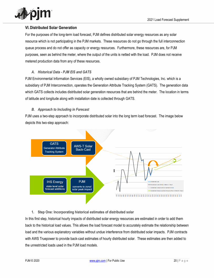
B. Approach to Including in Forecast PJM uses a two-step approach to incorporate distributed solar into the long term load forecast. The image below depicts this two-step approach:

1. Step One: Incorporating historical estimates of distributed solar In this first step, historical hourly impacts of distributed solar energy resources are estimated in order to add them back to the historical load values. This allows the load forecast model to accurately estimate the relationship between load and the various explanatory variables without undue interference from distributed solar impacts. PJM contracts with AWS Truepower to provide back-cast estimates of hourly distributed solar. These estimates are then added to the unrestricted loads used in the PJM load models.




2. Step Two: Incorporating historical estimates of distributed solar In the second step, PJM uses historical hourly estimates from AWS Truepower back to 1993. A daily capacity factor linked to the time of peak by season is used. For the summer season, hour ending 17 will be used. The solar output by weather scenario will vary in the same way the weather related to the historical weather scenario in the weather simulation varies.

VII. Plug-in Electric Vehicles The load forecast explicitly includes impacts from plug-in electric vehicles (PEV). The following is a description of the steps taken to include this adjustment in the forecast.Step 1: Compute the number of PEVs in the PJM Footprint

The number of registered plug-in electric vehicles by state is used as a starting point.

Forecasted PEV sales by U.S. census division are obtained from the Energy Information Administration’s Annual Energy Outlook and shared out to each state based on the state’s average share of census division PEV registrations.

Separately, vehicles are removed from the current stock based on their age; at a negligible rate initially, then growing until all vehicles from a given model year are removed after 20 years.

For a given year, a state’s forecast of PEVs is: Equation 27. State PEV Forecast

Existing PEV Stock + PEV Sales – Vehicle Retirements

Step 2: Compute PEV Peak and Energy Impacts

The peak impact of PEVs is a function of the prevalence of charging over the peak hour and the level of charger used. For a given year, a state’s peak forecast is: Equation 28. State PEV Peak Impact

(# Charging at Level 1 * 1.4 kW) + (# Charging at Level 2 * 7.7 kW)

The model assumes that the prevalence of charging over the peak hour will trend from 15% in 2020 to 5% in 2036, as incentives and technology combine to move charging to off-peak hours. The model also assumes that 80% of vehicles will use Level 1 chargers (which draw 1.4 kW) in 2020, trending to 0% by 2030, as Level 1 charging becomes insufficient to charge vehicles in a timely manner. Level 2 chargers are assumed to draw 7.7 kW.

For the energy forecast, PEVs are assumed to use 4,500 kWh per year, spread evenly across all months.

For both peak and energy, the state-level forecasts are allocated to zones based on the zone’s share of the RTO peak/energy.

This effort to capture PEV impacts only includes light duty vehicles, not large trucks, busses, or rail. PJM will work to add those impacts in future forecasts.




VIII. Forecast Adjustments PJM annually solicits information from its member Electric Distribution Companies (EDC) for large load shifts (either positive or negative) that are known to the EDC but may be unknown to PJM. Once the request has been verified per the guidelines in Attachment B of Manual 19, PJM works towards accounting for it in its load forecast. Each request is considered on a case-by-case basis, with particular caution paid to avoid double-counting anticipated load increases or decreases.

With each forecast adjustment, PJM seeks to incorporate the request into the end-use indices used to drive the load forecas, and then to quantify the MW impact on the forecast that is due to this request. What follows are descriptions of the analysis done. The corresponding data is posted with the supplemental materials.

A. APS FirstEnergy requested that PJM consider load additions for the APS zones related to significant growth in natural gas related facilities, as they have been in some form since PJM’s 2014 Load Forecast.

These facilities lie outside of the metropolitan areas used to define the economic footprint of the APS territory. As a result, this activity is not captured in the economic forecast used for APS, alleviating the risk of potential double-counting. APS provided energy and peak information on historical facilities as well as expectations for new facilities through 2025.

Given the nature of these facilities they are accounted for in the Industrial sector model.

Step 1: Compute status quo end-use indexes

Step 1 involves computing the end-use indexes without any additional treatment for the load request. This provides (1) information to determine the magnitude of the load adjustment and (2) the growth trajectory for the years beyond which there is an adjustment.

Step 2: Compute end-use indexes in the absence of load related to request

Subtract annual energy for these facilities from Industrial energy, and compute end-use indexes. Step 2 provides the underlying trend of the end-use indexes absent the load related to the request.

Step 3: Re-constitute end-use indexes with the load request

Using the results from Step 2, add the load associated with the request to the end-use indexes. This provides values for the end-use indexes through 2024.

Step 4: For years beyond 2025, grow end-use indexes according to what was obtained in Step 1

The load adjustment that is published as Table B-9 in the Load Forecast Report is the delta of the final forecast with and without adjustment (i.e. Step 1 versus Step 4).

B. BGE BGE requested that PJM consider their Conservation Voltage Reduction (CVR) program. This was first requested for consideration in the 2019 Load Forecast, and BGE has indicated that the program and its plan have not changed.




BGE’s program is “always on”, reducing load across its zone. Investment in the program began in 2014 and will be fully rolled out by 2022.

Because the program has been around since 2014, it has already been reducing load and thus would have some impact on the forecast. Thus to avoid double-counting, steps need to be taken to ensure that the CVR program is appropriately valued.

Step 1: Gross up energy data with any historical savings and calculate end-use indexes

Step 2: Reduce end-use indexes according to the percent savings

The load adjustment that is published as Table B-9 in the Load Forecast Report is the delta of the final forecast with an adjustment and a forecast without an adjustment (i.e. no steps taken to explicitly recognize the adjustment.).

C. COMED COMED requested that PJM consider their Voltage Optimization (VO) program. This was first requested for consideration in the 2019 Load Forecast, and COMED has indicated that the program and its plan have not changed. COMED’s program is “always on”, reducing load across its zone. Investment in the program began in 2018 and will be fully rolled out by 2026.

Because the program has been in place since 2018, it has already been reducing load and thus would have some impact on the forecast. Thus to avoid double-counting, steps need to be taken to ensure that the CVR program is appropriately valued.

Step 1: Gross up energy data with any historical savings and calculate end-use indexes

Step 2: Reduce end-use indexes according to the percent savings

The load adjustment that is published as Table B-9 in the Load Forecast Report is the delta of the final forecast with an adjustment and a forecast without an adjustment (i.e. no steps taken to explicitly recognize the adjustment).

D. Dominion (VEPCO) Dominion requested that PJM consider a forecast adjustment to account for the growth of data centers in northern Virginia. This adjustment has been in place in some form since the 2014 Load Forecast Report. The rationale for making an adjustment for data centers is that these centers have a load impact that is disproportionate with their economic impact. Data centers generally require minimum staffing and thus would not have a significant impact on economic variables, but do have a considerable impact on energy demand.

Dominion provides PJM with energy and peak information on historical facilities as well as expectations for new facilities through 2025. Given the nature of these facilities they are accounted for in the Commercial sector model.

Here are the steps taken to include this adjustment in the forecast.

Step 1: Compute status quo end-use indexes

Step 1 involves computing the end-use indexes without any additional treatment for the load request. This provides (1) information to determine the magnitude of the load adjustment and (2) the growth trajectory for the years beyond which there is an adjustment.




Step 2: Compute end-use indexes in the absence of load related to request

Subtract annual energy for these facilities from Commercial energy, and compute end-use indexes. Step 2 provides what the underlying trend would be absent the load request.

Step 3: Re-constitute end-use indexes with the load request

Using the results from Step 2, add the load associated with the request. Commercial contributes to Heat, Cool, and Other end-use indexes. Due to the nature of the load resembling that of what might be typically an industrial customer, all data center load is included in Other. This provides values through 2025.

Step 4: For years beyond 2025, grow end-use indexes according to what was obtained in Step 1

The Other end-use index is now trended using the growth pattern from Step 1.

The load adjustment that is published as Table B-9 in the Load Forecast Report is the delta of the final forecast with an adjustment and a forecast without an adjustment.

IX. Calendar Variables The forecast model includes a number of variables to capture calendar effects, represented primarily as either binary variables or fuzzy binary variables. Binary variables take a value of 1 or 0, whereas fuzzy binary variables have values ranging from 0 to 1. There is also a graduated variable to take into account the effect of Christmas lights.

Day of Week (=1 when that day, 0 otherwise)

Monday Tuesday Wednesday Thursday Friday Saturday

Month (=1 when that month, 0 otherwise)

January February March April May June

July August September October November

Holiday variables are coded such that they have values for more than one day, and for some holidays these values can differ year to year depending on the day of the week the holiday is observed. These variables are included because generally these days would be expected to have lower than normal loads.

MLK (Martin Luther King Day), PresDay (Presidents’ Day), MemDay (Memorial Day), and LaborDay (Labor Day)

Value

Day before Holiday 0.2

On Holiday 1

All other days 0




GoodFri (Good Friday) and Thanks (Thanksgiving Day)

Value

On Holiday 1

All other days 0

July4th (Independence Day)

Value by Day of Week

Monday Tuesday Wednesday Thursday Friday Saturday Sunday

July 2 0.10 0.00 0.00 0.15 0.15 0.10 0.15

July 3 0.70 0.25 0.15 0.20 0.80 0.20 0.20

July 4 1.00 1.00 0.80 1.00 1.00 0.40 0.30

July 5 0.80 0.15 0.15 0.25 0.70 0.30 0.15

July 6 0.00 0.00 0.00 0.00 0.10 0.20 0.00

All other days 0.00 0.00 0.00 0.00 0.00 0.00 0.00

FriAThanks (After Thanksgiving Day)

Value

On Holiday 1

Day After 0.2

All other days 0

XMasWkB4 (Week before Christmas Day)



December 21 0.33 0.33 0.33 0.50 0.50 0.50 0.33

December 22 0.50 0.50 0.67 0.67 0.80 0.50 0.50

December 23 1.00 0.67 0.67 1.00 1.00 0.67 0.67

All other days 0.00 0.00 0.00 0.00 0.00 0.00 0.00




XmasEve (Christmas Eve)



December 24 1.00 1.00 0.80 0.67 1.00 0.50 0.33

All other days 0.00 0.00 0.00 0.00 0.00 0.00 0.00

XMasDay (Christmas Day)



December 25 1.00 1.00 1.00 1.00 1.00 0.50 0.50

All other days 0.00 0.00 0.00 0.00 0.00 0.00 0.00

XMasWk (Time around Christmas and New Year’s)



December 26 1.00 0.67 0.67 0.67 1.00 0.20 0.25

December 27 0.25 0.33 0.33 0.33 0.50 0.20 0.15

December 28 0.25 0.33 0.33 0.33 0.33 0.20 0.15

December 29 0.33 0.33 0.33 0.33 0.33 0.20 0.15

December 30 0.80 0.50 0.33 0.50 0.50 0.25 0.25

January 2 0.80 0.15 0.33 0.33 0.67 0.25 0.15

January 3 0.00 0.15 0.00 0.15 0.15 0.15 0.15

January 4 0.00 0.00 0.00 0.00 0.15 0.00 0.00

All other days 0.00 0.00 0.00 0.00 0.00 0.00 0.00

NYEve (New Year’s Eve)



December 31 0.8 0.8 0.8 0.8 1.0 0.4 0.4




All other days 0.0 0.0 0.0 0.0 0.0 0.0 0.0

NYDay (New Year’s Day)



January 1 1.0 1.0 1.0 1.0 1.0 0.5 0.4

All other days 0.0 0.0 0.0 0.0 0.0 0.0 0.0

XMasLights (Christmas Lights Indicator)

This is a graduated variable that starts at 1 on the Friday after Thanksgiving, and increases by 1 each day until December 23.

X. Economics Zonal Assignment Economic variables come from Moody’s Analytics and geographical areas are assigned to zones per the table below.




XI. End-Use Inputs

A. Residential The Energy Information Administration’s (EIA) 2020 Annual Energy Outlook Reference Case is the starting point for data on residential end-uses. Residential end-uses fall into categories, which are then grouped according to weather and non-weather sensitive use types (i.e. Heating, Cooling, and Other). These categories are expressed as saturation rates (% of customers), efficiency metrics (use per year or efficiency term like Seasonal Energy Efficiency Ratio), and intensities (kWh per customer per year). Categories and groupings are as follows:

Zone Metro Area Name(s) or StateAE Atlantic City-Hammonton NJ, Ocean City NJ, Vineland-Bridgeton NJ

AEP

Elkhart-Goshen IN, Fort Wayne IN, Muncie IN, South Bend-Mishawaka IN-MI, Niles-Benton Harbor MI, Canton-Massillon OH, Columbus OH, Lima OH, Kingsport-Bristol TN, Blacksburg-Christiansburg-Radford, VA, Lynchburg VA, Roanoke VA, Beckley, WV, Charleston WV, Huntington-Ashland WV-KY-OH, Weirton-Steubenville WV-OH

APS Cumberland MD-WV, Hagerstown-Martinsburg MD-WV, Chambersburg-Waynesboro PA, State College PA, Winchester VA-WV, Morgantown WV, Parkersburg-Vienna WV

ATSI Akron OH, Cleveland-Elyria OH, Mansfield OH, Springfield OH, Toledo OH, Youngstown-Warren-Boardman OH-PA, Pittsburgh PA

BGE Baltimore-Columbia-Towson MD

COMED Chicago-Naperville-Arlington Heights IL, Elgin IL, Kankakee IL, Lake County-Kenosha County IL-WI, Rockford IL

DAY Dayton OHDEOK Cincinnati OH-KY-INDLCO Pittsburgh PADOM VirginiaDPL Dover DE, Wilmington DE-MD-NJ, Salisbury MD-DE

EKPC Cincinnati OH-KY-IN, Louisville/Jefferson County KY-IN, Elizabethtown-Fort Knox KY, Bowling Green KY, Lexington-Fayette KY, Huntington-Ashland WV-KY-OH

JCPL Camden NJ, Newark NJ-PA, Trenton NJ

METED Allentown-Bethlehem-Easton PA-NJ, East Stroudsburg PA, Gettysburg PA, Lebanon PA, Reading PA, York-Hanover PA,

PECO Montgomery County-Bucks County-Chester County PA, Philadelphia PAPENLC Altoona PA, Erie PA, Johnstown PAPEPCO Washington D.C., California-Lexington Park MD

PLAllentown-Bethlehem-Easton PA, Bloomsburg-Berwick PA, East Stroudsburg PA, Harrisburg-Carlisle PA, Lancaster PA, Scranton-Wilkes-Barre-Hazleton PA, Williamsport PA

PS Camden NJ, Newark NJ-PA, Trenton NJRECO Newark NJ-PAUGI Scranton-Wilkes-Barre-Hazleton PA




• Heating o Electric furnace and resistant room space heaters o Heat pump space heating o Ground-source heat pump space heating o Secondary heating o Furnace fans

• Cooling o Central air conditioning o Heat pump space cooling o Ground-source heat pump space cooling o Room air conditioners

• Other o Electric water heating o Electric cooking o Refrigerator o Second refrigerator o Freezer o Dishwasher o Electric clothes washer o Electric clothes dryer o TV sets o Lighting o Miscellaneous electric appliances

PJM receives this data at the Census division level through membership in Itron’s Energy Forecasting Group. PJM then supplements this with two pieces of information:

• State saturation estimates from the 2009 Residential Energy Consumption Survey • Zonal saturation estimates from

o American Electric Power – all appliance categories through 2018 o Allegheny Power – all appliance categories through 2016 o American Transmission Systems, Inc – all appliance categories through 2016 o Commonwealth Edison – all appliance categories for 2019 o Duke Energy Ohio and Kentucky – all appliance categories through 2014 o East Kentucky Power Cooperative – Heat Pumps for Heating and Cooling, Electric Furnaces,

Secondary Heating (Room Heating), Central A/C, Room Air Conditioners, and Water Heaters through 2013

o Jersey Central Power & Light – all appliance categories through 2016 o Metropolitan Edison – all appliance categories through 2016 o Pennsylvania Electric – all appliance categories through 2016 o Dominion Virginia Power – Heat Pumps for Cooling, Central A/C and Room Air Conditioners

through 2014

Zones are assigned to states and the forecasts are tied to Census Divisions. This allows the forecast to be influenced by the historical relative mix of appliances. For example, the Mid-Atlantic Census Division comprises Pennsylvania,




New Jersey and New York. However, each of these states has varying concentrations of Central Air Conditioning (New York has less than Pennsylvania or New Jersey). This information on historical appliance mix has an impact on the future mix and thus ultimately the residential end-use forecasts.

1. Efficiency of Residential Cooling Equipment When PJM added end-use measures into its model, stakeholder advice led us to make a modification to the efficiency measures of two segments: Central Air Conditioners and Heat Pumps4. Efficiency measures for these two items were based on the Seasonal Energy Efficiency Ratio (SEER), and the recommendation was that efficiency should be based on the Energy Efficiency Ratio (EER). The reason for the recommended switch was due to the calculation method of SEER not lining up well with conditions that would be expected at peak.

To make this adjustment, PJM annually has been collecting data on the SEER and EER of Central Air Conditioners and Heat Pumps to evaluate the relationship5. This exercise then allows us to convert the SEER provided efficiency figures in the Itron end-use files to EER calculated efficiency figures.

B. Commercial The EIA’s 2020 Annual Energy Outlook Reference Case is the starting point for data on commercial end-uses. Commercial end-uses fall into categories, which are then grouped according to weather and non-weather sensitive use types (i.e., Heating, Cooling, and Other). These categories are expressed as intensities (kWh per square foot per year). These categories and groupings are as follows:

• Heating • Cooling

4 See Navigant presentation from the November 30, 2015 Load Analysis Subcommittee meeting: https://www.pjm.com/-

/media/committees-groups/subcommittees/las/20151130/20151130-item-05-navigant-presentation.ashx 5 PJM obtains this data from the Air-Conditioning, Heating and Refrigeration Institute

Zone State Grouping for Benchmarking Census Division for ForecastAE New Jersey Mid-AtlanticAEP Indiana, Ohio East North CentralAPS Delaware, District of Columbia, Maryland, West Virginia South AtlanticATSI Indiana, Ohio East North CentralBGE Delaware, District of Columbia, Maryland, West Virginia South AtlanticCOMED Illinois East North CentralDAYTON Indiana, Ohio East North CentralDPL Delaware, District of Columbia, Maryland, West Virginia South AtlanticDQE Pennsylvania Mid-AtlanticDUKE Indiana, Ohio East North CentralEKPC Alabama, Kentucky, Mississippi East South CentralJCPL New Jersey Mid-AtlanticMETED Pennsylvania Mid-AtlanticPECO Pennsylvania Mid-AtlanticPENLC Pennsylvania Mid-AtlanticPEPCO Delaware, District of Columbia, Maryland, West Virginia South AtlanticPL Pennsylvania Mid-AtlanticPS New Jersey Mid-AtlanticRECO New Jersey Mid-AtlanticUGI Pennsylvania Mid-AtlanticVEPCO Virginia South Atlantic


https://www.pjm.com/-/media/committees-groups/subcommittees/las/20151130/20151130-item-05-navigant-presentation.ashx

https://www.pjm.com/-/media/committees-groups/subcommittees/las/20151130/20151130-item-05-navigant-presentation.ashx



• Other o Ventilation o Water Heating o Cooking o Refrigeration o Lighting o Office Equipment o Miscellaneous

PJM receives this data at the Census Division level through membership in Itron’s Energy Forecasting Group, and zones are assigned to Census Divisions using the same mapping as used for Residential end-uses.

XII. Additional Materials Additional materials are posted with the load forecast report. These can be found at https://www.pjm.com/planning/resource-adequacy-planning/load-forecast-dev-process. These include:

• Sector and End-Use Model Detail Spreadsheets o Residential Model o Commercial Model o Industrial Model o End-Use Indices

• Non-Weather Sensitive Model Detail Spreadsheets o Non-Weather Sensitive Estimates History o Non-Weather Sensitive Model Fit o Non-Weather Sensitive Forecast Model

• Final Model Detail Spreadsheets o Statistical Appendix

Contains parameter estimates and model statistics o Model Residuals

• Forecast Adjustments Detail Spreadsheet

• Weather Variables

• Input Assumptions o End-Use o Economics

• Model Accuracy


https://www.pjm.com/planning/resource-adequacy-planning/load-forecast-dev-process

Documents

2021 Load Forecast Supplement - PJM