Embed Size (px)
Citation preview

Astronomy & Astrophysics manuscript no. Planck˙Constraints˙on˙primordial˙non-Gaussianity˙2017 c© ESO 2019May 15, 2019
Planck 2018 results. IX. Constraints on primordial non-GaussianityPlanck Collaboration: Y. Akrami12,51,53, F. Arroja55, M. Ashdown60,4, J. Aumont89, C. Baccigalupi73, M. Ballardini19,37, A. J. Banday89,7,
R. B. Barreiro56, N. Bartolo25,57?, S. Basak79, K. Benabed50,88, J.-P. Bernard89,7, M. Bersanelli28,41, P. Bielewicz70,69,73, J. R. Bond6, J. Borrill10,86,F. R. Bouchet50,83, M. Bucher2,5, C. Burigana40,26,43, R. C. Butler37, E. Calabrese76, J.-F. Cardoso50, B. Casaponsa56, A. Challinor52,60,9,
H. C. Chiang22,5, L. P. L. Colombo28, C. Combet63, B. P. Crill58,8, F. Cuttaia37, P. de Bernardis27, A. de Rosa37, G. de Zotti38, J. Delabrouille2,J.-M. Delouis62, E. Di Valentino59, J. M. Diego56, O. Dore58,8, M. Douspis49, A. Ducout61, X. Dupac31, S. Dusini57, G. Efstathiou60,52, F. Elsner66,T. A. Enßlin66, H. K. Eriksen53, Y. Fantaye3,17, J. Fergusson9, R. Fernandez-Cobos56, F. Finelli37,43, M. Frailis39, A. A. Fraisse22, E. Franceschi37,
A. Frolov81, S. Galeotta39, K. Ganga2, R. T. Genova-Santos54,13, M. Gerbino34, J. Gonzalez-Nuevo14, K. M. Gorski58,91, S. Gratton60,52,A. Gruppuso37,43, J. E. Gudmundsson87,22, J. Hamann80, W. Handley60,4, F. K. Hansen53, D. Herranz56, E. Hivon50,88, Z. Huang77, A. H. Jaffe48,
W. C. Jones22, G. Jung25, E. Keihanen21, R. Keskitalo10, K. Kiiveri21,36, J. Kim66, N. Krachmalnicoff73, M. Kunz11,49,3, H. Kurki-Suonio21,36,J.-M. Lamarre82, A. Lasenby4,60, M. Lattanzi26,44, C. R. Lawrence58, M. Le Jeune2, F. Levrier82, A. Lewis20, M. Liguori25,57, P. B. Lilje53,
V. Lindholm21,36, M. Lopez-Caniego31, Y.-Z. Ma72,75,68, J. F. Macıas-Perez63, G. Maggio39, D. Maino28,41,45, N. Mandolesi37,26,A. Marcos-Caballero56, M. Maris39, P. G. Martin6, E. Martınez-Gonzalez56, S. Matarrese25,57,33, N. Mauri43, J. D. McEwen67, P.
D. Meerburg60,9,90, P. R. Meinhold23, A. Melchiorri27,46, A. Mennella28,41, M. Migliaccio30,47, M.-A. Miville-Deschenes1,49, D. Molinari26,37,44,A. Moneti50, L. Montier89,7, G. Morgante37, A. Moss78, M. Munchmeyer50, P. Natoli26,85,44, F. Oppizzi25, L. Pagano49,82, D. Paoletti37,43,
B. Partridge35, G. Patanchon2, F. Perrotta73, V. Pettorino1, F. Piacentini27, G. Polenta85, J.-L. Puget49,50, J. P. Rachen15, B. Racine53,M. Reinecke66, M. Remazeilles59, A. Renzi57, G. Rocha58,8, J. A. Rubino-Martın54,13, B. Ruiz-Granados54,13, L. Salvati49, M. Savelainen21,36,65,
D. Scott18, E. P. S. Shellard9, M. Shiraishi25,57,16, C. Sirignano25,57, G. Sirri43, K. Smith71, L. D. Spencer76, L. Stanco57, R. Sunyaev66,84,A.-S. Suur-Uski21,36, J. A. Tauber32, D. Tavagnacco39,29, M. Tenti42, L. Toffolatti14,37, M. Tomasi28,41, T. Trombetti40,44, J. Valiviita21,36, B. Van
Tent64, P. Vielva56, F. Villa37, N. Vittorio30, B. D. Wandelt50,88,24, I. K. Wehus53, A. Zacchei39, and A. Zonca74
(Affiliations can be found after the references)
Received xxxx, Accepted xxxxx
ABSTRACTWe analyse the Planck full-mission cosmic microwave background (CMB) temperature and E-mode polarization maps to obtain constraintson primordial non-Gaussianity (NG). We compare estimates obtained from separable template-fitting, binned, and optimal modal bispectrumestimators, finding consistent values for the local, equilateral, and orthogonal bispectrum amplitudes. Our combined temperature and polarizationanalysis produces the following final results: f local
NL = −0.9 ± 5.1; f equilNL = −26 ± 47; and f ortho
NL = −38 ± 24 (68 % CL, statistical). These resultsinclude the low-multipole (4 ≤ ` < 40) polarization data, not included in our previous analysis, pass an extensive battery of tests (with additionaltests regarding foreground residuals compared to 2015), and are stable with respect to our 2015 measurements (with small fluctuations, at the levelof a fraction of a standard deviation, consistent with changes in data processing). Polarization-only bispectra display a significant improvementin robustness; they can now be used independently to set primordial NG constraints with a sensitivity comparable to WMAP temperature-basedresults, and giving excellent agreement. In addition to the analysis of the standard local, equilateral, and orthogonal bispectrum shapes, we considera large number of additional cases, such as scale-dependent feature and resonance bispectra, isocurvature primordial NG, and parity-breakingmodels, where we also place tight constraints but do not detect any signal. The non-primordial lensing bispectrum is, however, detected withan improved significance compared to 2015, excluding the null hypothesis at 3.5σ. Beyond estimates of individual shape amplitudes, we alsopresent model-independent reconstructions and analyses of the Planck CMB bispectrum. Our final constraint on the local primordial trispectrumshape is glocal
NL = (−5.8 ± 6.5) × 104 (68 % CL, statistical), while constraints for other trispectrum shapes are also determined. Exploiting thetight limits on various bispectrum and trispectrum shapes, we constrain the parameter space of different early-Universe scenarios that generateprimordial NG, including general single-field models of inflation, multi-field models (e.g., curvaton models), models of inflation with axionfields producing parity-violation bispectra in the tensor sector, and inflationary models involving vector-like fields with directionally-dependentbispectra. Our results provide a high-precision test for structure-formation scenarios, showing complete agreement with the basic picture of theΛCDM cosmology regarding the statistics of the initial conditions, with cosmic structures arising from adiabatic, passive, Gaussian, and primordialseed perturbations.
Key words. Cosmology: observations – Cosmology: theory – cosmic background radiation – early Universe – inflation – Methods: data analysis
Contents
1 Introduction 2
2 Models 32.1 General single-field models of inflation . . . . . 32.2 Multi-field models . . . . . . . . . . . . . . . . 32.3 Isocurvature non-Gaussianity . . . . . . . . . . . 42.4 Running non-Gaussianity . . . . . . . . . . . . . 4
? Corresponding author: Nicola Bartolo [email protected]
2.4.1 Local-type scale-dependent bispectrum . 52.4.2 Equilateral type scale-dependent bispec-
trum . . . . . . . . . . . . . . . . . . . 52.5 Oscillatory bispectrum models . . . . . . . . . . 5
2.5.1 Resonance and axion monodromy . . . . 62.5.2 Scale-dependent oscillatory features . . . 6
2.6 Non-Gaussianity from excited initial states . . . . 62.7 Directional-dependent NG . . . . . . . . . . . . 72.8 Parity-violating tensor non-Gaussianity moti-
vated by pseudo-scalars . . . . . . . . . . . . . . 7
3 Estimators and data analysis procedures 8
1
arX
iv:1
905.
0569
7v1
[as
tro-
ph.C
O]
14
May
201
9

Planck Collaboration: Constraints on primordial non-Gaussianity
3.1 Bispectrum estimators . . . . . . . . . . . . . . 83.1.1 KSW and skew-C` estimators . . . . . . 83.1.2 Running of primordial non-Gaussianity . 93.1.3 Modal estimators . . . . . . . . . . . . . 103.1.4 Binned bispectrum estimator . . . . . . . 10
3.2 Data set and analysis procedures . . . . . . . . . 103.2.1 Data set and simulations . . . . . . . . . 103.2.2 Data analysis details . . . . . . . . . . . 10
4 Non-primordial contributions to the CMB bispec-trum 114.1 Non-Gaussianity from the lensing bispectrum . . 114.2 Non-Gaussianity from extragalactic point sources 13
5 Results 145.1 Constraints on local, equilateral, and orthogonal
fNL . . . . . . . . . . . . . . . . . . . . . . . . . 145.2 Further bispectrum shapes . . . . . . . . . . . . 16
5.2.1 Isocurvature non-Gaussianity . . . . . . 165.2.2 Running non-Gaussianity . . . . . . . . 185.2.3 Resonance and axion monodromy . . . . 195.2.4 Scale-dependent oscillatory features . . . 205.2.5 High-frequency feature and resonant-
model estimator . . . . . . . . . . . . . . 205.2.6 Equilateral-type models and the effec-
tive field theory of inflation . . . . . . . . 205.2.7 Models with excited initial states (non-
Bunch-Davies vacua) . . . . . . . . . . . 235.2.8 Direction-dependent primordial non-
Gaussianity . . . . . . . . . . . . . . . . 235.2.9 Parity-violating tensor non-Gaussianity
motivated by pseudo-scalars . . . . . . . 235.3 Bispectrum reconstruction . . . . . . . . . . . . 25
5.3.1 Modal bispectrum reconstruction . . . . 255.3.2 Binned bispectrum reconstruction . . . . 25
6 Validation of Planck results 266.1 Dependence on foreground-cleaning method . . . 27
6.1.1 Comparison between fNL measurements . 276.1.2 Comparison between reconstructed bis-
pectra . . . . . . . . . . . . . . . . . . . 296.2 Testing noise mismatch . . . . . . . . . . . . . . 326.3 Effects of foregrounds . . . . . . . . . . . . . . . 34
6.3.1 Non-Gaussianity of the thermal dustemission . . . . . . . . . . . . . . . . . 34
6.3.2 Impact of the tSZ effect . . . . . . . . . . 356.4 Dependence on sky coverage . . . . . . . . . . . 356.5 Dependence on multipole number . . . . . . . . 376.6 Summary of validation tests . . . . . . . . . . . 37
7 Limits on the primordial trispectrum 39
8 Implications for early-Universe physics 408.1 General single-field models of inflation . . . . . 408.2 Multi-field models . . . . . . . . . . . . . . . . 418.3 Non-standard inflation models . . . . . . . . . . 428.4 Alternatives to inflation . . . . . . . . . . . . . . 438.5 Inflationary interpretation of CMB trispectrum
results . . . . . . . . . . . . . . . . . . . . . . . 43
9 Conclusions 44
1. Introduction
This paper, one of a set associated with the 2018 release(also known as “PR3”) of data from the Planck1 mission(Planck Collaboration I 2018), presents the data analysis andconstraints on primordial non-Gaussianity (NG) obtained us-ing the Legacy Planck cosmic microwave background (CMB)maps. It also includes some implications for inflationary mod-els driven by the 2018 NG constraints. This paper updates theearlier study based on the temperature data from the nom-inal Planck operations period, including the first 14 monthsof observations (Planck Collaboration XXIV 2014, hereafterPCNG13), and a later study that used temperature data and afirst set of polarization maps from the full Planck mission—29and 52 months of observations for the HFI (High FrequencyInstrument) and LFI (Low Frequency Instrument), respec-tively (Planck Collaboration XVII 2016, hereafter PCNG15).The analysis described in this paper sets the most stringent con-straints on primordial NG to date, which are near what is ul-timately possible from using only CMB temperature data. Theresults of this paper are mainly based on the measurementsof the CMB angular bispectrum, complemented with the nexthigher-order NG correlation function, i.e., the trispectrum. Fornotations and conventions relating to (primordial) bispectra andtrispectra we refer the reader to the two previous Planck pa-pers on primordial NG (PCNG13; PCNG15). This paper alsocomplements the precise characterization of inflationary mod-els (Planck Collaboration X 2018) and cosmological parameters(Planck Collaboration VI 2018), with specific statistical estima-tors that go beyond the constraints on primordial power spectra.It also complements the statistical and isotropy tests on CMBanisotropies of Planck Collaboration VII (2018), focusing on theinterpretation of specific, well motivated, non-Gaussian mod-els of inflation. These models span from the irreducible min-imal amount of primordial NG predicted by standard single-field models of slow-roll inflation, to various classes of infla-tionary models that constitute the prototypes of extensions of thestandard inflationary picture and of physically motivated mech-anisms able to generate a higher level of primordial NG mea-surable in the CMB anisotropies. This work establishes the mostrobust constraints on some of the most well-known and studiedtypes of primordial NG, namely the local, equilateral, and or-thogonal shapes. Moreover, this 2018 analysis includes a bettercharacterization of the constraints coming from CMB polariza-tion data. Besides focusing on these major goals, we re-analyse avariety of other NG signals, investigating also some new aspectsof primordial NG. For example, we perform for the first timean analysis of the running of NG using Planck data in the con-text of some well defined inflationary models. Additionally, weconstrain primordial NG predicted by theoretical scenarios onwhich much attention has been focused recently, such as, bispec-trum NG generated in the tensor (gravitational wave) sector. Fora detailed analysis of oscillatory features that combines powerspectrum and bispectrum constraints see Planck Collaboration X(2018). As in the last data release (“PR2”), as well as extractingthe constraints on NG amplitudes for specific shapes, we alsoprovide a model-independent reconstruction of the CMB angular
1 Planck (http://www.esa.int/Planck) is a project of theEuropean Space Agency (ESA) with instruments provided by two sci-entific consortia funded by ESA member states and led by PrincipalInvestigators from France and Italy, telescope reflectors providedthrough a collaboration between ESA and a scientific consortium ledand funded by Denmark, and additional contributions from NASA(USA).
2
Planck Collaboration: Constraints on primordial non-Gaussianity
bispectrum by using various methods. Such a reconstruction canhelp in pinning down interesting features in the CMB bispectrumsignal beyond those captured by existing parameterizations.
The paper is organized as follows. In Sect. 2 we recall themain primordial NG models tested in this paper. Section 3 brieflydescribes the bispectrum estimators that we use, as well as de-tails of the data set and our analysis procedures. In Sect. 4 wediscuss detectable non-primordial contributions to the CMB bis-pectrum, namely those arising from lensing and point sources. InSect. 5 we constrain fNL for the local, equilateral, and orthogo-nal bispectra. We also report the results for scale-dependent NGmodels and other selected bispectrum shapes, including NG inthe tensor (primordial gravitational wave) sector; in this sectionreconstructions and model-independent analyses of the CMBbispectrum are also provided. In Sect. 6 these results are vali-dated through a series of null tests on the data, with the goal ofassessing the robustness of the results. This includes in particulara first analysis of Galactic dust and thermal SZ residuals. PlanckCMB trispectrum limits are obtained and discussed in Sect. 7. InSect. 8 we derive the main implications of Planck’s constraintson primordial NG for some specific early Universe models. Weconclude in Sect. 9.
2. Models
Primordial NG comes in with a variety of shapes, correspondingto well motivated classes of inflationary model. For each class,a common physical mechanism is responsible for the generationof the corresponding type of primordial NG. Below we brieflysummarize the main types of primordial NG that are constrainedin this paper, providing the precise shapes that are used for dataanalysis. For more details about specific realizations of inflation-ary models within each class, see the previous two Planck pa-pers on primordial NG (PCNG13; PCNG15) and reviews (e.g.,Bartolo et al. 2004a; Liguori et al. 2010; Chen 2010b; Komatsu2010; Yadav & Wandelt 2010). We give a more expanded de-scription only of those shapes of primordial NG analysed herefor the first time with Planck data (e.g., running of primordialNG).
2.1. General single-field models of inflation
The parameter space of single-field models is well de-scribed by the so called equilateral and orthogonal templates(Creminelli et al. 2006; Chen et al. 2007b; Senatore et al. 2010).The equilateral shape is
BequilΦ
(k1, k2, k3) = 6A2 f equilNL
×
− 1
k4−ns1 k4−ns
2
−1
k4−ns2 k4−ns
3
−1
k4−ns3 k4−ns
1
−2
(k1k2k3)2(4−ns)/3
+
1
k(4−ns)/31 k2(4−ns)/3
2 k4−ns3
+ 5 perms.
, (1)
while the orthogonal NG is described by
BorthoΦ (k1, k2, k3) = 6A2 f ortho
NL
×
− 3
k4−ns1 k4−ns
2
−3
k4−ns2 k4−ns
3
−3
k4−ns3 k4−ns
1
−8
(k1k2k3)2(4−ns)/3
+
3
k(4−ns)/31 k2(4−ns)/3
2 k4−ns3
+ 5 perms.
. (2)
Here the potential Φ is defined in relation to the comoving curva-ture perturbation ζ by Φ ≡ (3/5)ζ on superhorizon scales (thuscorresponding to Bardeen’s gauge-invariant gravitational poten-tial (Bardeen 1980) during matter domination on superhorizonscales). PΦ(k) = A/k4−ns is the Bardeen gravitational poten-tial power spectrum, with normalization A and scalar spectralindex ns. A typical example of this class is provided by mod-els of inflation where there is a single scalar field driving in-flation and generating the primordial perturbations, character-ized by a non-standard kinetic term or more general higher-derivative interactions. In the first case the inflaton Lagrangianis L = P(X, φ), where X = gµν∂µφ ∂νφ, with at most onederivative on φ (Chen et al. 2007b). Different higher-derivativeinteractions of the inflaton field characterize, ghost inflation(Arkani-Hamed et al. 2004) or models of inflation based onGalileon symmetry (e.g., Burrage et al. 2011). The two am-plitudes f equil
NL and f orthoNL usually depend on the sound speed
cs at which the inflaton field fluctuations propagate and ona second independent amplitude measuring the inflaton self-interactions. The Dirac-Born-Infeld (DBI) models of inflation(Silverstein & Tong 2004; Alishahiha et al. 2004) are a string-theory-motivated example of the P(X, φ) models, predicting analmost equilateral type NG with f equil
NL ∝ c−2s for cs 1. More
generally, the effective field theory (EFT) approach to infla-tionary perturbations (Cheung et al. 2008; Senatore et al. 2010;Bartolo et al. 2010a) yields NG shapes that can be mapped intothe equilateral and orthogonal template basis. The EFT approachallows us to draw generic conclusions about single-field in-flation. We will discuss them using one example in Sect. 8.Nevertheless, we shall also explicitly search for such EFTshapes, analysing their exact non-separable predicted shapes,BEFT1 and BEFT2, along with those of DBI, BDBI, and ghost infla-tion, Bghost (Arkani-Hamed et al. 2004).
2.2. Multi-field models
The bispectrum for multi-field models is typically of the localtype2
BlocalΦ (k1, k2, k3) = 2 f local
NL
[PΦ(k1)PΦ(k2)
+ PΦ(k1)PΦ(k3) + PΦ(k2)PΦ(k3)]
= 2A2 f localNL
1
k4−ns1 k4−ns
2
+ cycl.
. (3)
This usually arises when more scalar fields drive inflation andgive rise to the primordial curvature perturbation (“multiple-field inflation”), or when extra light scalar fields, different fromthe inflaton field driving inflation, determine (or contributeto) the final curvature perturbation. In these models initialisocurvature perturbations are transferred on super-horizonscales to the curvature perturbations. Non-Gaussianities ifpresent are transferred too. This, along with nonlineari-ties in the transfer mechanism itself, is a potential sourceof significant NG (Bartolo et al. 2002; Bernardeau & Uzan2002; Vernizzi & Wands 2006; Rigopoulos et al. 2006,2007; Lyth & Rodriguez 2005; Tzavara & van Tent 2011;Jung & van Tent 2017). The bispectrum of Eq. (3) mainly
2 See, e.g., Byrnes & Choi (2010) for a review on this type ofmodel in the context of primordial NG. Early papers discussing pri-mordial local bispectra given by Eq. (3) include Falk et al. (1993),Gangui et al. (1994), Gangui & Martin (2000), Verde et al. (2000),Wang & Kamionkowski (2000), and Komatsu & Spergel (2001).
3

Planck Collaboration: Constraints on primordial non-Gaussianity
correlates large- with small-scale modes, peaking in the“squeezed” configurations k1 k2 ≈ k3. This is a conse-quence of the transfer mechanism taking place on superhorizonscales and thus generating a localized point-by-point primor-dial NG in real space. The curvaton model (Mollerach 1990;Linde & Mukhanov 1997; Enqvist & Sloth 2002; Lyth & Wands2002; Moroi & Takahashi 2001) is a clear example where lo-cal NG is generated in this way (e.g., Lyth & Wands 2002;Lyth et al. 2003; Bartolo et al. 2004d). In the minimal adi-abatic curvaton scenario f local
NL = (5/4rD) − 5rD/6 − 5/3(Bartolo et al. 2004d,c), in the case when the curvaton fieldpotential is purely quadratic (Lyth & Wands 2002; Lyth et al.2003; Lyth & Rodriguez 2005; Malik & Lyth 2006; Sasaki et al.2006). Here rD = [3ρcurv/(3ρcurv + 4ρrad)]D represents the“curvaton decay fraction” at the epoch of the curvaton decay,employing the sudden decay approximation. Significant NGcan be produced (Bartolo et al. 2004d,c) for low values of rD; adifferent modelling of the curvaton scenario has been discussedby Linde & Mukhanov (2006) and Sasaki et al. (2006). Weupdate the limits on both models in Sect. 8, using the local NGconstraints. More general models with a curvaton-like spectatorfield have also been intensively investigated recently (see, e.g.,Torrado et al. 2018). Notice that through a similar mechanismto the curvaton mechanism, local bispectra can be generatedfrom nonlinear dynamics during the preheating and reheat-ing phases (Enqvist et al. 2005; Chambers & Rajantie 2008;Barnaby & Cline 2006; Bond et al. 2009) or due to fluctuationsin the decay rate or interactions of the inflaton field, as realizedin modulated (p)reheating and modulated hybrid inflationarymodels (Kofman 2003; Dvali et al. 2004a,b; Bernardeau et al.2004; Zaldarriaga 2004; Lyth 2005; Salem 2005; Lyth & Riotto2006; Kolb et al. 2006; Cicoli et al. 2012). We will also explorewhether there is any evidence for dissipative effects during warminflation, with a signal which changes sign in the squeezed limit(see e.g., Bastero-Gil et al. 2014).
2.3. Isocurvature non-Gaussianity
In most of the models mentioned in this section the fo-cus is on primordial NG in the adiabatic curvature perturba-tion ζ. However, in inflationary scenarios with multiple scalarfields, isocurvature perturbation modes can be produced aswell. If they survive until recombination, these will then con-tribute not only to the power spectrum, but also to the bis-pectrum, producing in general both a pure isocurvature bis-pectrum and mixed bispectra because of the cross-correlationbetween isocurvature and adiabatic perturbations (Komatsu2002; Bartolo et al. 2002; Komatsu et al. 2005; Kawasaki et al.2008; Langlois et al. 2008; Kawasaki et al. 2009; Hikage et al.2009; Langlois & Lepidi 2011; Langlois & van Tent 2011;Kawakami et al. 2012; Langlois & van Tent 2012; Hikage et al.2013a,b).
In the context of the ΛCDM cosmology, there are at the timeof recombination four possible distinct isocurvature modes (inaddition to the adiabatic mode), namely the cold-dark-matter(CDM) density, baryon-density, neutrino-density, and neutrino-velocity isocurvature modes (Bucher et al. 2000). However, thebaryon isocurvature mode behaves identically to the CDMisocurvature mode, once rescaled by factors of Ωb/Ωc, so wewill only consider the other three isocurvature modes in this pa-per. Moreover, we will only investigate isocurvature NG of thelocal type, since this is the most relevant case in multi-field infla-tion models, which we require in order to produce isocurvaturemodes. We will also limit ourselves to studying just one type
of isocurvature mode (considering each of the three types sepa-rately) together with the adiabatic mode, to avoid the number offree parameters becoming so large that no meaningful limits canbe derived. Finally, for simplicity we assume the same spectralindex for the primordial isocurvature power spectrum and theadiabatic-isocurvature cross-power spectrum as for the adiabaticpower spectrum, again to reduce the number of free parameters.As shown by Langlois & van Tent (2011), under these assump-tions we have in general six independent fNL parameters: theusual purely adiabatic one; a purely isocurvature one; and fourcorrelated ones.
The primordial isocurvature bispectrum templates are a gen-eralization of the local shape in Eq. (3):
BIJK(k1, k2, k3) = 2 f I,JKNL PΦ(k2)PΦ(k3) + 2 f J,KI
NL PΦ(k1)PΦ(k3)
+ 2 f K,IJNL PΦ(k1)PΦ(k2), (4)
where I, J,K label the different adiabatic and isocurvaturemodes. The invariance under the simultaneous exchange of twoof these indices and the corresponding momenta means thatf I,JKNL = f I,KJ
NL , which reduces the number of independent pa-rameters from eight to six in the case of two modes (and ex-plains the notation with the comma). The different CMB bis-pectrum templates derived from these primordial shapes varymost importantly in the different types of radiation transferfunctions that they contain. For more details, see in particularLanglois & van Tent (2012).
An important final remark is that, unlike the case of thepurely adiabatic mode, polarization improves the constraints onthe isocurvature NG significantly, up to a factor of about 6 as pre-dicted by Langlois & van Tent (2011, 2012) and confirmed bythe 2015 Planck analysis (PCNG15). The reason for this is thatwhile the isocurvature temperature power spectrum (to which thelocal bispectrum is proportional) becomes very quickly negligi-ble compared to the adiabatic one as ` increases (already around`≈ 50 for CDM), the isocurvature polarization power spectrumremains comparable to the adiabatic one to much smaller scales(up to `≈ 200 for CDM). Hence there are many more polar-ization modes than temperature modes that are relevant for de-termining these isocurvature fNL parameters. For more details,again see Langlois & van Tent (2012).
2.4. Running non-Gaussianity
We briefly describe inflationary models that predict a mildlyscale-dependent bispectrum, which is also known in the liter-ature as the running of the bispectrum (see e.g., Chen 2005;Liguori et al. 2006; Kumar et al. 2010; Byrnes et al. 2010b,a;Shandera et al. 2011). In inflationary models this running is asnatural as the running of the power spectrum, i.e., the spectralindex ns. Other models with strong scale dependence, e.g., oscil-latory models, will be discussed in Sect. 2.5. Further possibili-ties for strong scale dependence exist (see e.g., Khoury & Piazza2009; Riotto & Sloth 2011), but we will not consider these in ourstudy. The simplest model (single-field slow-roll, with canoni-cal action and initial conditions) predicts that both the ampli-tude and scale dependence are of the order of the slow-roll pa-rameters (this is true except in some very particular models,see, e.g., Chen et al. (2013)), i.e., they are small and currentlynot observable. However, other elaborate but theoretically well-motivated models make different predictions and these can beused to confirm or exclude such models. Measuring the run-ning of the non-Gaussianity parameters with scale is impor-tant because this running carries information about, for instance,
4

Planck Collaboration: Constraints on primordial non-Gaussianity
the number of inflationary fields and their interactions. Thisinformation may not be accessible with the power spectrumalone. The first constraints on the running of a local modelwere obtained with WMAP7 data in Becker & Huterer (2012).Forecasts of what would be feasible with future data were per-formed by for instance LoVerde et al. (2008), Sefusatti et al.(2009), Becker et al. (2011), Giannantonio et al. (2012), andBecker et al. (2012).
2.4.1. Local-type scale-dependent bispectrum
We start by describing models with a local-type mildly scale-dependent bispectrum. Assuming that there are multiple scalarfields during inflation with canonical kinetic terms, that theircorrelators are Gaussian at horizon crossing, and using the slow-roll approximation and the δN formalism, Byrnes et al. (2010a)found a quite general expression for the power spectrum of theprimordial potential perturbation:
PΦ(k) =2π2
k3 PΦ(k) =2π2
k3
∑ab
Pab(k), (5)
where the indexes a, b run over the different scalar fields.The nonlinearity parameter then reads (Byrnes et al. 2010a)
fNL(k1, k2, k3) =BΦ(k1, k2, k3)
2[PΦ(k1)PΦ(k2) + 2 perms.
]=
∑abcd(k1k2)−3Pac(k1)Pbd(k2) fcd(k3) + 2 perms.
(k1k2)−3P(k1)P(k2) + 2 perms.,
(6)
where the last line is the general result valid for any number ofslow-roll fields. The functions fcd (as well as the functions Pab)can be parameterized as power laws. In the general case, fNL canalso be written as
fNL(k1, k2, k3) =∑ab
f abNL
(k1k2)nmulti,a k3+n f ,ab
3 + 2 perms.
k31 + k3
2 + k33
, (7)
where nmulti,a and n f ,ab are parameters of the models that areproportional to the slow-roll parameters. It is clear that in thegeneral case there are too many parameters to be constrained.Instead we will consider two simpler cases, which will be amongthe three models of running non-Gaussianity that will be anal-ysed in Sect. 5.2.2.
Firstly, when the curvature perturbation originates from onlyone of the scalar fields (e.g., as in the simplest curvaton scenario)the bispectrum simplifies to (Byrnes et al. 2010a)
BΦ(k1, k2, k3) ∝ (k1k2)ns−4knNG3 + 2 perms. (8)
In this case
fNL(k1, k2, k3) = f pNL
k3+nNG1 + k3+nNG
2 + k3+nNG3
k31 + k3
2 + k33
, (9)
where nNG is the running parameter which is sensitive to thethird derivative of the potential. If the field producing the pertur-bations is not the inflaton field but an isocurvature field subdom-inant during inflation, then neither the spectral index measure-ment nor the running of the spectral index are sensitive to thethird derivative. Therefore, those self-interactions can uniquelybe probed by the running of fNL.
The second class of models are two-field models whereboth fields contribute to the generation of the perturbations butthe running of the bispectrum is still given by one parame-ter only (by choosing some other parameters appropriately) as(Byrnes et al. 2010a)
BΦ(k1, k2, k3) ∝ (k1k2)ns−4+(nNG/2) + 2 perms. (10)
Comparing the two templates (8) and (10) one sees that thereare multiple ways to generalize (with one extra parameter) theconstant local fNL model, even with the same values for fNL andnNG. If one is able to distinguish observationally between thesetwo shapes then one could find out whether the running origi-nated from single or multiple field effects for example.
Byrnes et al. (2010a) further assumed that|n fNL ln (kmax/kmin) | 1. In our case, ln (kmax/kmin) <∼ 8and nNG can be at most of order 0.1. If the observationalconstraints on nNG using the previous theoretical templates turnout to be weaker, then one cannot use those constraints to limitthe fundamental parameters of the models because the templatesare being used in a region where they are not applicable.However, from a phenomenological point of view, we wishto argue that the previous templates are still interesting casesof scale-dependent bispectra, even in that parameter region.Byrnes et al. (2010a) also computed the running of the trispectraamplitudes τNL and gNL. For general single-source modelsthey showed that nτNL = 2nNG, analogous to the well-known
consistency relation τNL(k) =(
65 fNL(k)
)2, providing a useful
consistency check.
2.4.2. Equilateral type scale-dependent bispectrum
General single-field models that can produce large bispectra hav-ing a significant correlation with the equilateral template alsopredict a mild running non-Gaussianity. A typical example isDBI-inflation, as studied, e.g., by Chen (2005) and Chen et al.(2007b), with a generalization within the effective field theoryof inflation in Bartolo et al. (2010c). Typically in these models arunning NG arises of the form
fNL → f ∗NL
(k1 + k2 + k3
3kpiv
)nNG
, (11)
where nNG is the running parameter and kpiv is a pivot scaleneeded to constrain the amplitude. For example, in the casewhere the main contribution comes from a small sound speed ofthe inflaton field, nNG = −2s, where s = cs/(Hcs), and there-fore running NG allows us to constrain the time dependenceof the sound speed.3 The equilateral NG with a running of thetype given in Eq. (11) is a third type of running NG analysed inSect. 5.2.2 (together with the local single-source model of Eq. 8and the local two-field model of Eq. 10). We refer the reader toSect. 3.1.2 for the details on the methodology adopted to analysethese models.
2.5. Oscillatory bispectrum models
Oscillatory power spectrum and bispectrum signals are possi-ble in a variety of well-motivated inflationary models, including
3 This would help in further breaking (via primordial NG) somedegeneracies among the parameters determining the curvature powerspectrum in these modes. For a discussion and an analysis of this type,see Planck Collaboration XXII (2014) and Planck Collaboration XX(2016).
5

Planck Collaboration: Constraints on primordial non-Gaussianity
those with an imposed shift symmetry or if there are sharp fea-tures in the inflationary potential. Our first Planck temperature-only non-Gaussian analysis (PCNG13) included a search for thesimplest resonance and feature models, while the second Plancktemperature with polarization analysis (PCNG15) substantiallyexpanded the frequency range investigated, while also encom-passing a much wider class of oscillatory models. These phe-nomenological bispectrum shapes had free parameters designedto capture the main properties of the key extant oscillatory mod-els, thus surveying for any oscillatory signals present in the dataat high significance. Our primary purpose here is to use the re-vised Planck 2018 data set to determine the robustness of oursecond analysis, so we only briefly introduce the models studied,referring the reader to our previous work (PCNG15) for moredetailed information.
2.5.1. Resonance and axion monodromy
Motivated by the UV completion problem facing large-field in-flation, effective shift symmetries can be used to preserve theflat potentials required by inflation, with a prime example be-ing the periodically modulated potential of axion monodromymodels. This periodic symmetry can cause resonances duringinflation, imprinting logarithmically-spaced oscillations in thepower spectrum, bispectrum and beyond (Flauger et al. 2010;Hannestad et al. 2010; Flauger & Pajer 2011). For the bispec-trum, to a good approximation, these models yield the simpleoscillatory shape (see e.g., Chen 2010b)
BresΦ (k1, k2, k3) =
6A2 f resNL
(k1k2k3)2 sin[ω ln(k1 + k2 + k3) + φ
], (12)
where the constant ω is an effective frequency associated withthe underlying periodicity of the model and φ is a phase. Theunits for the wavenumbers, ki, are arbitrary as any specific choicecan be absorbed into the phase which is marginalised over in ourresults. There are more general resonance models that naturallycombine properties of inflation inspired by fundamental theory,notably a varying sound speed cs or an excited initial state. Thesetend to modulate the oscillatory signal on K = k1 + k2 + k3 con-stant slices, with either equilateral or flattened shapes, respec-tively (see e.g., Chen 2010a), which we take to have the form
S eq(k1, k2, k3) =k1k2k3
k1k2k3, S flat = 1 − S eq , (13)
where k1 ≡ k2 + k3 − k1. Note that S eq correlates closely withthe equilateral shape in (1) and S flat with the orthogonal shape in(2), since the correction from the spectral index ns is small. Theresulting generalized resonance shapes for which we search arethen
Bres−eq(k1, k2, k3) ≡ S eq(k1, k2, k3) × Bres(k1, k2, k3) ,
Bres−flat(k1, k2, k3) ≡ S flat(k1, k2, k3) × Bres(k1, k2, k3) . (14)
This analysis does not exhaust resonant models associated witha non-Bunch-Davies initial state, which can have a more sharplyflattened shape (“enfolded” models), but it should help iden-tify this tendency if present in the data. In addition, the dis-cussion in Flauger et al. (2017) showed that the resonant fre-quency can “drift” slowly over time with a correction term tothe frequency being proposed, but again we leave that for fu-ture analysis. Finally, we note that there are multifield modelsin which sharp corner-turning can result in residual oscillationswith logarithmic spacing, thus mimicking resonance models
(Achucarro et al. 2011; Battefeld et al. 2013). However, theseoscillations are more strongly damped and can be searched forby modulating the resonant shape (Eq. 12) with a suitable enve-lope, as discussed for feature models below.
2.5.2. Scale-dependent oscillatory features
Sharp features in the inflationary potential can generate oscilla-tory signatures (Chen et al. 2007a), as can rapid variations in thesound speed cs or fast turns in a multifield potential. Narrowfeatures in the potential induce a corresponding signal in thepower spectrum, bispectrum, and trispectrum; to a first approx-imation, the oscillatory bispectrum has a simple sinusoidal be-haviour given by (Chen et al. 2007a)
Bfeat(k1, k2, k3) =6A2 f feat
NL
(k1k2k3)2 sin[ω(k1 + k2 + k3) + φ
], (15)
where ω is a frequency determined by the specific featureproperties and φ is a phase. The wavenumbers ki are in unitsof Mpc−1. A more accurate analytic bispectrum solution hasbeen found that includes a damping envelope taking the form(Adshead et al. 2012)
BK2 cos(k1, k2, k3) =6A2 f K2 cos
NL
(k1k2k3)2 K2D(αωK) cos(ωK) , (16)
where K = k1 + k2 + k3 and the envelope function is given byD(αωK) = αω/
(K sinh(αωK)
). Here, the model-dependent pa-
rameter α determines the large wavenumber cutoff, with α = 0for no envelope in the limit of an extremely narrow feature.Oscillatory signals generated instead by a rapidly varying soundspeed cs take the form
BK sin(k1, k2, k3) =6A2 f K sin
NL
(k1k2k3)2 K D(αωK) sin(ωK) . (17)
In order to encompass the widest range of physically-motivated feature models, we will also modulate the predictedsignal (Eq. 15) with equilateral and flattened shapes, as definedin Eq. (13), i.e.,
Bfeat−eq(k1, k2, k3) ≡ S eq(k1, k2, k3) × Bfeat(k1, k2, k3) , (18)
Bfeat−flat(k1, k2, k3) ≡ S flat(k1, k2, k3) × Bfeat(k1, k2, k3) . (19)
Like our survey of resonance models, this allows the feature sig-nal to have arisen in inflationary models with (slowly) varyingsound speeds or with excited initial states. In the latter case, it isknown that very narrow features can mimic non-Bunch Daviesbispectra with a flattened or enfolded shape (Chen et al. 2007a).
2.6. Non-Gaussianity from excited initial states
Inflationary perturbations generated by “excited” initial states(non-Bunch-Davies vacuum states) generically create non-Gaussianities with a distinct enfolded shape (see e.g., Chen et al.2007b; Holman & Tolley 2008; Meerburg et al. 2009), that is,where the bispectrum signal is dominated by flattened con-figurations with k1 + k2 ≈ k3 (and cyclic permutations). Inthe present analysis, we investigate all the non-Bunch-Davies(NBD) models discussed in the previous Planck non-Gaussianpapers, where explicit equations can be found for the bis-pectrum shape functions. In the original analysis (PCNG13),we described: the vanilla flattened shape model Bflat ∝ S flat al-ready given in Eq. (13); a more realistic flattened model BNBD
6

Planck Collaboration: Constraints on primordial non-Gaussianity
(Chen et al. 2007b) from power-law k-inflation, with excitationsgenerated at time τc, yielding an oscillation period (and cut-off) kc ≈ (τccs)−1; the two leading-order shapes for excitedcanonical single-field inflation labelled BNBD1-cos and BNBD2-cos
(Agullo & Parker 2011); and a non-oscillatory sharply flattenedmodel BNBD3, with large enhancements from a small soundspeed cs (Chen 2010b). In the second (temperature plus polar-ization) analysis (PCNG15), we also studied additional NBDshapes including a sinusoidal version of the original NBD bis-pectrum BNBD-sin (Chen 2010a), and similar extensions for thesingle-field excited models (Agullo & Parker 2011), labelledBNBD1−sin and BNBD2−sin, with the former dominated by oscil-latory squeezed configurations.
2.7. Directional-dependent NG
The standard local bispectrum in the squeezed limit (k1 k2 ≈
k3) has an amplitude that is the same for all different angles be-tween the large-scale mode with wavevector k1 and the small-scale modes parameterized by wavevector ks = (k2 − k3)/2.More generally, we can consider “anisotropic” bispectra, inthe sense of an angular dependence on the orientation of thelarge-scale and small-scale modes, where in the squeezed limitthe bispectrum depends on all even powers of µ = k1 · ks
(where k = k/k, and all odd powers vanish by symmetryeven out of the squeezed limit). Expanding the squeezed bis-pectrum into Legendre polynomials with even multipoles L, theL > 0 shapes then be used to cleanly isolate new physical ef-fects. In the literature it is more common to expand in the angleµ12 = k1 · k2, which makes some aspects of the analysis sim-pler while introducing non-zero odd L moments (since they nolonger vanish when defined using the non-symmetrized small-scale wavevector). We then parameterize variations of local NGusing (Shiraishi et al. 2013a):
BΦ(k1, k2, k3) =∑
L
cL[PL(µ12)PΦ(k1)PΦ(k2) + 2 perms.] , (20)
where PL(µ) is the Legendre polynomial with P0 = 1, P1 = µ,and P2 = 1
2 (3µ2 − 1). For instance, in the L = 1 case the shape isgiven by
BL=1Φ (k1, k2, k3) =
2A2 f L=1NL
(k1k2k3)2
k23
k21k2
2
(k21 + k2
2 − k23) + 2 perms.
.(21)
Bispectra of the directionally dependent class in general peak inthe squeezed limit (k1 k2 ≈ k3), but they feature a non-trivialdependence on the parameter µ12 = k1 · k2. The local NG tem-plate corresponds to ci = 2 fNLδi0. The nonlinearity parametersf LNL are related to the cL coefficients by c0 = 2 f L=0
NL , c1 = −4 f L=1NL ,
and c2 = −16 f L=2NL . The L = 1 and 2 shapes are characterized by
sharp variations in the flattened limit, e.g., for k1 +k2 ≈ k3, whilein the squeezed limit, L = 1 is suppressed, unlike L = 2, whichgrows like the local bispectrum shape (i.e., the L = 0 case).
Bispectra of the type in Eq. (20) can arise in different in-flationary models, e.g., models where anisotropic sources con-tribute to the curvature perturbation. Bispectra of this type areindeed a general and unavoidable outcome of models that sus-tain long-lived superhorizon gauge vector fields during infla-tion (Bartolo et al. 2013a). A typical example is the case ofthe inflaton field ϕ coupled to the kinetic term F2 of a U(1)gauge field Aµ, via the interaction term I2(ϕ)F2, where Fµν =
∂µAν − ∂νAµ and the coupling I2(ϕ)F2 can allow for scale invari-ant vector fluctuations to be generated on superhorizon scales
(Barnaby et al. 2012; Bartolo et al. 2013a).4 Primordial mag-netic fields sourcing curvature perturbations can also generatea dependence on both µ and µ2 (Shiraishi 2012). The I2(ϕ)F2
models predict c2 = c0/2, while models where the primor-dial curvature perturbations are sourced by large-scale mag-netic fields produce c0, c1, and c2. The so-called “solid infla-tion” models (Endlich et al. 2013; see also Bartolo et al. 2013b;Endlich et al. 2014; Sitwell & Sigurdson 2014; Bartolo et al.2014) also predict bispectra of the form Eq. (20). In this casec2 c0 (Endlich et al. 2013, 2014). Inflationary models thatbreak rotational invariance and parity also generate this kind ofNG with the specific prediction c0 : c1 : c2 = 2 : −3 : 1(Bartolo et al. 2015). Therefore, measurements of the ci coef-ficients can test for the existence of primordial vector fields dur-ing inflation, fundamental symmetries, or non-trivial structureunderlying the inflationary model (as in solid inflation).
Recently much attention has been focused on the possibil-ity of testing the presence of higher-spin particles via their im-prints on higher-order inflationary correlators. Measuring pri-mordial NG can allow us to pin down masses and spins ofthe particle content present during inflation, making inflationa powerful cosmological collider (Chen 2010b; Chen & Wang2010; Noumi et al. 2013; Arkani-Hamed & Maldacena 2015;Baumann et al. 2018; Arkani-Hamed et al. 2018). In the case oflong-lived superhorizon higher-spin (effectively massless or par-tially massless higher spin fields) bispectra like in Eq. (20) aregenerated, where even coefficients up to cn=2s are excited, s be-ing the spin of the field (Franciolini et al. 2018). A structuresimilar to Eq. (20) arises in the case of massive spin particles,where the coefficients ci has a specific non-trivial dependence onthe mass and spin of the particles (Arkani-Hamed & Maldacena2015; Baumann et al. 2018; Moradinezhad Dizgah et al. 2018).
2.8. Parity-violating tensor non-Gaussianity motivated bypseudo-scalars
In some inflationary scenarios involving the axion field, thereare chances to realize the characteristic NG signal in the tensor-mode sector. In these cases a non-vanishing bispectrum of pri-mordial gravitational waves, Bs1 s2 s3
h , arises via the nonlinear in-teraction between the axion and the gauge field. Its magnitudevaries depending on the shape of the axion-gauge coupling, and,in the best-case scenario, the tensor mode can be comparablein size to or dominate the scalar mode (Cook & Sorbo 2013;Namba et al. 2016; Agrawal et al. 2018).
The induced tensor bispectrum is polarized as B+++h
B++−h , B+−−
h , B−−−h (because the source gauge field is maximallychiral), and peaked at around the equilateral limit (because thetensor-mode production is a subhorizon event). Its size is there-fore quantified by the so-called tensor nonlinearity parameter,
f tensNL ≡ lim
ki→k
B+++h (k1, k2, k3)
Fequilζ (k1, k2, k3)
, (22)
with Fequilζ ≡ (5/3)3Bequil
Φ/ f equil
NL .In this paper we constrain f tens
NL by measuring the CMB tem-perature and E-mode bispectra computed from B+++
h (for theexact shape of B+++
h see PCNG15). By virtue of their parity-violating nature, the induced CMB bispectra have non-vanishingsignal for not only the even but also the odd `1 + `2 + `3 triplets
4 Notice that indeed these models generate bispectra (and powerspectra) that break statistical isotropy and, after an angle average, thebispectrum takes the above expression (Eq. 20).
7

Planck Collaboration: Constraints on primordial non-Gaussianity
(Shiraishi et al. 2013b). Both are investigated in our analysis,yielding more unbiased and accurate results. The Planck 2015paper (PCNG15) found a best limit of f tens
NL = (0 ± 13) × 102
(68% CL), from the foreground-cleaned temperature and high-pass filtered E-mode data, where the E-mode information for` < 40 was entirely discarded in order to avoid foreground con-tamination. This paper updates those limits with additional data,including large-scale E-mode information.
3. Estimators and data analysis procedures
3.1. Bispectrum estimators
We give here a short description of the data-analysis proceduresused in this paper. For additional details, we refer the reader tothe primordial NG analysis associated with previous Planck re-leases (PCNG13; PCNG15) and to references provided below.
For a rotationally invariant CMB sky and even parity bis-pectra (as is the case for combinations of T and E), the angularbispectrum can be written as
〈aX1`1m1
aX2`2m2
aX3`3m3〉 = G`1`2`3
m1m2m3bX1X2X3`1`2`3
, (23)
where bX1X2X3`1`2`3
defines the “reduced bispectrum,” and G`1`2`3m1m2m3 is
the Gaunt integral, i.e., the integral over solid angle of the prod-uct of three spherical harmonics,
G`1`2`3m1m2m3
≡
∫Y`1m1 (n) Y`2m2 (n) Y`3m3 (n) d2 n . (24)
The Gaunt integral (which can be expressed as a product ofWigner 3 j-symbols) enforces rotational symmetry. It satisfiesboth a triangle inequality and a limit given by some maximumexperimental resolution `max. This defines a tetrahedral domainof allowed bispectrum triplets, `1, `2, `3.
In order to estimate the fNL value for a given primordialshape, we need to compute a theoretical prediction of the corre-sponding CMB bispectrum ansatz bth
`1`2`3and fit it to the observed
3-point function (see e.g., Komatsu & Spergel 2001).Optimal cubic bispectrum estimators were first discussed
in Heavens (1998). It was then shown that, in the limit ofsmall NG, the optimal polarized fNL estimator is described by(Creminelli et al. 2006)
fNL =1N
∑Xi,X′i
∑`i,mi
∑`′i ,m
′i
G `1 `2 `3m1m2m3
bX1X2X3, th`1`2`3
[(C−1`1m1,`
′1m′1
)X1X′1 aX′1`′1m′1
×(C−1`2m2,`
′2m′2
)X2X′2 aX′2`′2m′2
(C−1`3m3,`
′3m′3
)X3X′3 aX′3`′3m′3
]−
[ (C−1`1m1,`2m2
)X1X2(C−1`3m3,`
′3m′3
)X3X′3 aX′3`′3m′3
+ cyclic], (25)
where the normalization N is fixed by requiring unit response tobth`1`2`3
when fNL = 1. C−1 is the inverse of the block matrix:
C =
(CTT CT E
CET CEE
). (26)
The blocks represent the full TT, TE, and EE covariance matri-ces, with CET being the transpose of CT E . CMB a`m coefficients,bispectrum templates, and covariance matrices in the previousrelation are assumed to include instrumental beam and noise.
As shown in the formula above, these estimators are alwayscharacterized by the presence of two distinct contributions. One
is cubic in the observed multipoles, and computes the correlationbetween the observed bispectrum and the theoretical templatebth`1`2`3
. This is generally called the “cubic term” of the estimator.The other is instead linear in the observed multipoles. Its role isthat of correcting for mean-field contributions to the uncertain-ties, generated by the breaking of rotational invariance, due tothe presence of a mask or to anisotropic/correlated instrumentalnoise (Creminelli et al. 2006; Yadav et al. 2008).
Performing the inverse-covariance filtering operation im-plied by Eq. (25) is numerically very demanding (Smith et al.2009; Elsner & Wandelt 2012). An alternative, simplified ap-proach, is that of working in the “diagonal covariance approx-imation,” yielding (Yadav et al. 2007)
fNL =1N
∑Xi,X′i
∑`i,mi
G `1 `2 `3m1m2m3
(C−1)X1X′1`1
(C−1)X2X′2`2
(C−1)X3X′3`3
bX1X2X3, th`1`2`3
×
[aX′1`1m1
aX′2`2m2
aX′3`3m3− C
X′1X′2`1m1,`2m2
aX′3`3m3− C
X′1X′3`1m1,`3m3
aX′2`2m2
−CX′2X′3`2m2,`3m3
aX′1`1m1
]. (27)
Here, C−1` represents the inverse of the following 2 × 2 matrix:
C` =
(CTT` CT E
`
CET` CEE
`
). (28)
As already described in PCNG13, we find that this simpli-fication, while avoiding the covariance-inversion operation, stillleads to uncertainties that are very close to optimal, provided thatthe multipoles are pre-filtered using a simple diffusive inpaintingmethod. As in previous analyses, we stick to this approach here.
A brute-force implementation of Eq. (27) would require theevaluation of all the possible bispectrum configurations in ourdata set. This is completely unfeasible, as it would scale as ` 5
max.The three different bispectrum estimation pipelines employed inthis analysis are characterized by the different approaches usedto address this issue.
Before describing these methods in more detail in the fol-lowing sections, we would like to stress here, the importanceof having these multiple approaches. The obvious advantage isthat this redundancy enables a stringent cross-validation of ourresults. There is, however, much more than that, as differentmethods allow a broad range of applications, beyond fNL esti-mation, such as, for example, model-independent reconstructionof the bispectrum in different decomposition domains, precisecharacterization of spurious bispectrum components, monitoringdirection-dependent NG signals, and so on.
3.1.1. KSW and skew-C` estimators
Komatsu-Spergel-Wandelt (KSW) and skew-C` estimators(Komatsu et al. 2005; Munshi & Heavens 2010) can be appliedto bispectrum templates that can be factorized, i.e., they can bewritten or well approximated as a linear combination of sepa-rate products of functions. This is the case for the standard local,equilateral, and orthogonal shapes, which cover a large range oftheoretically motivated scenarios. The idea is that factorizationleads to a massive reduction in computational time, via reductionof the three-dimensional summation over `1, `2, `3 into a productof three separate one-dimensional sums over each multipole.
The skew-C` pipeline differs from KSW essentially in that,before collapsing the estimate into the fNL parameter, it initiallydetermines the so called “bispectrum-related power spectrum”
8

Planck Collaboration: Constraints on primordial non-Gaussianity
(in short, “skew-C`”) function (see Munshi & Heavens 2010) fordetails). The slope of this function is shape-dependent, whichmakes the skew-C` extension very useful to separate and monitormultiple and spurious NG components in the map.
3.1.2. Running of primordial non-Gaussianity
In the previous 2015 analysis, the KSW pipeline was used onlyto constrain the separable local, equilateral, orthogonal, andlensing templates. In the current analysis we extend its scope byadding the capability to constrain running of non-Gaussianity,encoded in the spectral index of the nonlinear amplitude fNL,denoted nNG.
In our analysis we consider both the two local running tem-plates, described by Eqs. (8) and (10) in Sect. 2.4.1, and the gen-eral parametrizazion for equilateral running of Sect. 2.4.2, whichreads:
fNL → f ∗NL
(k1 + k2 + k3
3kpiv
)nNG
, (29)
where nNG is the running parameter and kpiv is a pivot scaleneeded to constrain the amplitude. Contrary to the two local run-ning shapes this expression is not explicitly separable. To makeit suitable for the KSW estimator (e.g., to preserve the factor-izability over ki), we can use a Schwinger parametrization andrearrange it as
fNL →f ∗NL
3knNGpiv
ksum
Γ(1 − nNG)
∫ ∞
0dt t−nNG e−tksum , (30)
where ksum = k1 + k2 + k3.Alternatively, but not equivalently, factorizability can be pre-
served by replacing the arithmetic mean of the three wavenum-bers with the geometric mean (Sefusatti et al. 2009):
fNL → f ∗NL
k1k2k3
k3piv
nNG
3
. (31)
Making one of these substitutions immediately yields thescale-dependent version of any bispectrum shape. Analysis inOppizzi et al. (2018) has shown strong correlation between thetwo templates, where the former behaves better numerically andis the template of choice for the running in this analysis.
A generalization of the local model, taking into account thescale dependence of fNL, can be found in Byrnes et al. (2010a),as summarized in Sect. 2.4.1.
Unlike fNL, the running parameter nNG cannot be estimatedvia direct template fitting. The optimal estimation procedure,developed in Becker & Huterer (2012) and extended to all thescale-dependent shapes treated here in Oppizzi et al. (2018), isbased instead on the reconstruction of the likelihood function,with respect nNG. The method exploits the KSW estimator toobtain estimates of f ∗NL for different values of the running, usingexplicitly separable bispectrum templates. With these values inhand, the running parameter probability density function (PDF)is computed from its analytical expression.
The computation of the marginalized likelihood depends onthe choice of the prior distributions; in Becker & Huterer (2012)and Oppizzi et al. (2018) a flat prior on f ∗NL was assumed. Thisprior depends on the choice of the arbitrary pivotal scale kpiv,since a flat prior on f ∗NL defined at a certain scale, correspondsto a non-flat prior for another scale. The common solution isto select the pivot scale that minimizes the correlation betweenthe parameters. This is in general a good choice, and would
work properly in the case of a significant detection of a bis-pectrum signal. In the absence of a clear detection, however, itis worth noting some caveats. Since the range of scales avail-able is obviously finite, a fit performed at a certain pivot scalewill tend to favour particular values of nNG. Therefore, there isnot a perfectly “fair” scale for the fit. As a consequence, sta-tistical artefacts can affect the estimated constraints in the caseof low significance of the measured f ∗NL central value. To pre-vent this issue, we resort to two additional approaches that makethe final nNG PDF pivot independent: the implementation of aparametrization invariant Jeffreys prior; and frequentist likeli-hood profiling. Assuming that the bispectrum configurations fol-low a Gaussian distribution, the likelihood can be written as (seeBecker & Huterer 2012, for a derivation)
L(nNG, f ∗NL) ∝ exp
−N( f ∗NL − fNL)2
2
exp
f 2NLN2
, (32)
where fNL is the value of the NG amplitude recovered from theKSW estimator for a fixed nNG value of the running, and N isthe KSW normalization factor. Integrating this expression withrespect to f ∗NL we obtain the marginalized likelihood. Assuminga constant prior we obtain
L(nNG) ∝1√
Nexp
f 2NLN2
. (33)
The Jeffreys prior is defined as the square root of the determi-nant of the Fisher information matrix I( fNL, nNG). In the case ofseparable scale-dependent bispectra, the Fisher matrix is
Iα,β ≡∑
`1≤`2≤`3
(2`1 + 1)(2`2 + 1)(2`3 + 1)4π
(`1 `2 `30 0 0
)2
×1
σ2`1`2`3
∂b`1`2`3
∂θα
∂b`1`2`3
∂θβ, (34)
where θα and θβ correspond to f ∗NL or nNG (depending on thevalue of the index), b`1`2`3 is the reduced bispectrum, and thematrix is a Wigner-3j symbol.
We search an expression for the posterior distributionmarginalized over f ∗NL. Assuming the Jeffreys prior for both pa-rameters and integrating over fNL, we obtain the marginalizedposterior
P(nNG) ∝
fNL
√2πN
exp
f 2NLN2
erf
fNL
√N2
+2N
×
√det(I( f ∗NL = 1, nNG)). (35)
The implementation of this expression in the estimator isstraightforward; the only additional step is the numerical com-putation of the Fisher matrix determinant for each value of nNGconsidered. The derived expression is independent of the pivotscale.
Alternatively, in the frequentist approach, instead ofmarginalizing over f ∗NG, the likelihood is sampled along its max-imum for every nNG value. For fixed nNG, the maximum like-lihood f ∗NG is given exactly by the KSW estimator fNL. FromEq. (32), we see that for this condition the first exponential is setto 1 (since f ∗NG = fNL at the maximum), and the profile likeli-hood reduces to
L(nNG) ∝ exp
f 2NLN2
. (36)
9

Planck Collaboration: Constraints on primordial non-Gaussianity
Notice that this expression also does not depend on the pivotscale. We will additionally use this expression to perform a like-lihood ratio test between our scale-dependent models and thestandard local and equilateral shapes.
3.1.3. Modal estimators
Modal estimators (Fergusson et al. 2010, 2012) are based onconstructing complete, orthogonal bases of separable bispectrumtemplates (“bispectrum modes”) and finding their amplitudes byfitting them to the data. This procedure can be made fast, due tothe separability of the modes, via a KSW type of approach. Thevector of estimated mode amplitudes is referred to as the “modespectrum.” This mode spectrum is theory independent and it con-tains all the information that needs to be extracted from the data.It is also possible to obtain theoretical mode spectra, by expand-ing primordial shapes in the same modal basis used to analysethe data. This allows us to measure fNL for any given primordialbispectrum template, by correlating the theoretical mode vec-tors, which can be quickly computed for any shape, with the datamode spectrum. This feature makes modal techniques ideal foranalyses of a large number of competing models. Also importantis that non-separable bispectra are expanded with arbitrary preci-sion into separable basis modes. Therefore the treatment of non-separable shapes is always numerically efficient in the modal ap-proach. Finally, the data mode spectrum can be used, in combi-nation with measured mode amplitudes, to build linear combi-nations of basis templates, which provide a model-independentreconstruction of the full data bispectrum. This reconstruction isof course smoothed in practice, since we use a finite number ofmodes. The modal bispectrum presented here follows the sameapproach as in 2015. In particular we use two modal pipelines,“Modal 1” and “Modal 2,” characterized both by a different ap-proach to the decomposition of polarized bispectra and by a dif-ferent choice of basis, as detailed in PCNG13, PCNG15, and atthe end of Sect. 3.2.2.
3.1.4. Binned bispectrum estimator
The “Binned” bispectrum estimator (Bucher et al. 2010, 2016)is based on the exact optimal fNL estimator, in combinationwith the observation that many bispectra of interest are relativelysmooth functions in ` space. This means that data and templatescan be binned in ` space with minimal loss of information, butwith large computational gains. As a consequence, no KSW-likeapproach is required, and the theoretical templates and obser-vational bispectra are computed and stored completely indepen-dently, and only combined at the very last stage in a sum overthe bins to obtain fNL. This has several advantages: the methodis fast; it is easy to test additional shapes without having to re-run the maps; the bispectrum of a map can be studied on itsown in a non-parametric approach (a binned reconstruction ofthe full data bispectrum is provided, which can additionally besmoothed); and the dependence of fNL on ` can be investigatedfor free, simply by leaving out bins from the final sum. All ofthese advantages are used to good effect in this paper.
The Binned bispectrum estimator was described in more de-tail in the papers associated with the 2013 and 2015 Planck re-leases, and full details can be found in Bucher et al. (2016). Theone major change made to the Binned estimator code comparedto the 2015 release concerns the computation of the linear cor-rection term, required to make the estimator optimal in the casethat rotational invariance is broken, as it is in the Planck anal-
ysis because of the mask and anisotropic noise. The version ofthe code used in 2015, while fast to compute the linear correc-tion for a single map, scaled poorly with the number of maps, asthe product of the data map with all the Gaussian maps squaredhad to be recomputed for each data map. Hence computing realerrors, which requires analysing a large set of realistic simula-tions, was slow. The new code can precompute the average ofthe Gaussian maps squared, and then quickly apply it to all thedata maps. For the full Planck analysis, with errors based on 300simulations, one gains an order of magnitude in computing time(see Bucher et al. 2016, for more details).
3.2. Data set and analysis procedures
3.2.1. Data set and simulations
For our temperature and polarization data analyses we usethe Planck 2018 CMB maps, as constructed with the fourcomponent-separation methods, SMICA, SEVEM, NILC, andCommander (Planck Collaboration IV 2018). We also makemuch use of simulated maps, for several different purposes,from computing errors to evaluating the linear mean-fieldcorrection terms for our estimators, as well as for per-forming data-validation checks. Where not otherwise speci-fied we will use the FFP10 simulation data set described inPlanck Collaboration II (2018), Planck Collaboration III (2018),and Planck Collaboration IV (2018), which are the most realis-tic Planck simulations currently available. The maps we con-sider have been processed through the same four component-separation pipelines. The same weights used by the differentpipelines on actual data have been adopted to combine differentsimulated frequency channels.
Simulations and data are masked using the common masksof the Planck 2018 release in temperature and polarization; seePlanck Collaboration IV (2018) for a description of how thesemasks have been produced. The sky coverage fractions are,fsky = 0.779 in temperature and fsky = 0.781 in polarization.
3.2.2. Data analysis details
Now we describe the setup adopted for the analysis of Planck2018 data by the four different fNL estimators described earlierin this section.
In order to smooth mask edges and retain optimality, as ex-plained earlier, we inpaint the mask via a simple diffusive in-painting method (Bucher et al. 2016). First, we fill the maskedregions with the average value of the non-masked part of themap. Then we replace each masked pixel with the average valueof its neighbours and iterate this 2000 times. This is exactly thesame procedure as adopted in 2013 and 2015.
Linear correction terms and fNL errors are obtained fromthe FFP10 simulations, processed through the four component-separation pipelines. To this end, all pipelines use all the avail-able 300 FFP10 noise realizations, except both modal estima-tors, which use only 160 maps (in order to speed up the com-putation). The good convergence of the modal pipelines with160 maps was thoroughly tested in previous releases. There, weshowed with a large number of tests on realistic simulations thatthe level of agreement between all our bispectrum estimatorswas perfectly consistent with theoretical expectations. Accuratetests have found some mismatch between the noise levels in thedata and that of the FFP10 simulations (Planck Collaboration III2018; Planck Collaboration IV 2018). This is roughly at the 3 %level in the noise power spectrum at ` ≈ 2000, in temperature,
10
Planck Collaboration: Constraints on primordial non-Gaussianity
and at the percent level, in polarization. We find (see Sect. 6.2for details) that this mismatch does not play a significant role inour analysis, and can safely be ignored.
All theoretical quantities (e.g., bispectrum templates andlensing bias) are computed assuming the Planck 2018 best-fit cosmology and making use of the CAMB computer code5
(Lewis et al. 2000) to compute radiation transfer functionsand theoretical power spectra. The HEALPix computer code6
(Gorski et al. 2005) is used to perform spherical harmonic trans-forms.
As far as temperature is concerned, we maintain the samemultipole ranges as in the 2013 and 2015 analyses, which is2 ≤ ` ≤ 2000 for the KSW and modal estimators and 2 ≤` ≤ 2500 for the Binned estimator. The different choice of `maxdoes not produce any significant effect on the results, since the2000 < ` ≤ 2500 range is noise dominated and the measuredvalue of fNL remains very stable in that range, as confirmedby validation tests discussed in Sect. 6. The angular resolution(beam FWHM) of both the cleaned temperature and polarizationmaps is 5 arcminutes.
The main novelty of the current analysis is the use of the low-` polarization multipoles that were not exploited in 2015 (` <40 polarization multipoles were removed by means of a high-pass filter). More precisely, KSW and modal estimators workin the polarization multipole range 4 ≤ ` ≤ 1500, while theBinned estimator considers 4 ≤ ` ≤ 2000. For the same reasonsas above, this different choice of `max does not have any impacton the results.
The choice of using `min = 4 for polarization, thus remov-ing the first two polarization multipoles, is instead dictated bythe presence of some anomalous results in tests on simulations.When ` = 2 and ` = 3 are included, we observe some smallbias arising in the local fNL measurement extracted from FFP10maps, together with a spurious increase of the uncertainties. Wealso notice larger discrepancies between the different estimationpipelines than expected from either theoretical arguments or pre-vious validation tests on simulations. This can be ascribed to thepresence of some small level of non-Gaussianity in the polariza-tion noise at very low `. We stress that the choice of cutting thefirst two polarization multipoles does not present any particularissue, since it is performed a priori, before looking at the data (asopposed to the simulations), and generates an essentially negli-gible loss of information.
In addition, the Binned bispectrum estimator removes fromthe analysis all bispectrum T EE configurations (i.e., those in-volving one temperature mode and two polarization modes) withthe temperature mode in the bin [2, 3]. This is again motivated byoptimality considerations: with these modes included the com-puted errors are much larger than the optimal Fisher errors, whileafter removing them the errors are effectively optimal. As errorsare computed from simulations, this is again an a priori choice,made before looking at the data. It is not clear why only theBinned bispectrum estimator requires this additional removal,but of course the estimators are all quite different, with differ-ent sensitivities, which is exactly one of the strengths of havingmultiple estimators for our analyses.
The Binned bispectrum estimator uses a binning that is iden-tical to the one in 2015, with 57 bins. The boundary values ofthe bins are 2, 4, 10, 18, 30, 40, 53, 71, 99, 126, 154, 211,243, 281, 309, 343, 378, 420, 445, 476, 518, 549, 591, 619, 659,700, 742, 771, 800, 849, 899, 931, 966, 1001, 1035, 1092, 1150,
5 http://camb.info/6 http://healpix.sourceforge.net/
1184, 1230, 1257, 1291, 1346, 1400, 1460, 1501, 1520, 1540,1575, 1610, 1665, 1725, 1795, 1846, 1897, 2001, 2091, 2240,and 2500 (i.e., the first bin is [2, 3], the second [4, 9], etc., whilethe last one is [2240, 2500]). This binning was determined in2015 by minimizing the increase in the theoretical variance forthe primordial shapes due to the binning.
As in our 2015 analysis, we use two different polarizedmodal estimators. The “Modal 1” pipeline expands separatelythe TTT, EEE, TTE, and EET bispectra (Shiraishi et al. 2019).It then writes the estimator normalization in separable expandedform and estimates fNL via a direct implementation of Eq. (27).The “Modal 2” pipeline uses a different approach (see Fergusson2014, for details). It first orthogonalizes T and E multipolesto produce new, uncorrelated, aT
`m and aE`m coefficients. It then
builds uncorrelated bispectra out of these coefficients, which areconstrained independently, simplifying the form and reducingthe number of terms in the estimator. However, the rotation pro-cedure does not allow a direct estimation of the EEE bispectrum.Direct EEE reconstruction is generally useful for validation pur-poses and can be performed with the Modal 1 estimator.
As in 2015, Modal 1 is used to study in detail the local, equi-lateral, and orthogonal shapes, as well as to perform a large num-ber of validation and robustness tests. Modal 2 is mostly dedi-cated to a thorough study of non-standard shapes having a largeparameter space (like oscillatory bispectra). The two pipelinesare equipped with modal bases optimized for their respectivepurposes. Modal 1 uses 600 polynomial modes, augmented withradial modes extracted from the KSW expansion of the local,equilateral, and orthogonal templates, in order to speed up con-vergence for these shapes. The Modal 2 expansion uses a higher-resolution basis, including 2000 polynomial modes and a Sachs-Wolfe local template, to improve efficiency in the squeezed limit.
For oscillating non-Gaussianities we also use two special-ized estimators (Munchmeyer et al. 2014, 2015) that specificallytarget the high-frequency range of shapes, which cannot be cov-ered by the modal pipelines or the Binned estimator. Both ofthese estimators are equivalent to those used in PCNG15.
4. Non-primordial contributions to the CMBbispectrum
In this section we investigate those non-primordial contributionsto the CMB bispectrum that we can detect in the cleaned maps,namely lensing and extragalactic point sources. These then po-tentially have to be taken into account when determining the con-straints on the various primordial NG shapes in Sect. 5. On theother hand, the study of other non-primordial contaminants (thatwe do not detect in the cleaned maps) is part of the validationwork in Sect. 6.
4.1. Non-Gaussianity from the lensing bispectrum
CMB lensing generates a significant CMB bispectrum(Hanson & Lewis 2009; Mangilli & Verde 2009; Lewis et al.2011; Mangilli et al. 2013). In temperature, this is due to corre-lations between the lensing potential and the integrated Sachs-Wolfe (ISW; Sachs & Wolfe 1967) contribution to the CMBanisotropies. In polarization, the dominant contribution insteadcomes from correlations between the lensing potential and Emodes generated by scattering at reionization. Both the ISWand reionization contributions affect large scales, while lens-ing is a small-scale effect, so that the resulting bispectrapeak on squeezed configurations. Therefore, they can signif-
11

Planck Collaboration: Constraints on primordial non-Gaussianity
icantly contaminate primordial NG measurements, especiallyfor the local shape. It has been known for a while that fora high-precision experiment like Planck the effect is largeenough that it must be taken into account. The temperature-only 2013 Planck results (PCNG13, Planck Collaboration XIX2014, Planck Collaboration XVII 2014) showed the first detec-tion of the lensing CMB temperature bispectrum and the asso-ciated bias. This was later confirmed in the 2015 Planck results(PCNG15, Planck Collaboration XXI 2016) both for T -only andfor the full T+E results. The template of the lensing bispectrum7
is given by (Hu 2000; Lewis et al. 2011),
bX1X2X3, lens`1`2`3
= f lensNL
(CX2φ`2
CX1X3`3
f X1`1`2`3
+ CX3φ`3
CX1X2`2
f X1`1`3`2
+ CX1φ`1
CX2X3`3
f X2`2`1`3
+ CX3φ`3
CX1X2`1
f X2`2`3`1
+ CX1φ`1
CX2X3`2
f X3`3`1`2
+ CX2φ`2
CX1X3`1
f X3`3`2`1
)(37)
where the Xi are either T or E. The tilde on CXiX j
`indicates
that it is the lensed power spectrum, while CTφ`
and CEφ`
are thetemperature/polarization-lensing potential cross-power spectra.The functions f T,E
`1`2`3are defined by
f T`1`2`3
=12[`2(`2 + 1) + `3(`3 + 1) − `1(`1 + 1)
],
f E`1`2`3
=12
[`2(`2 + 1) + `3(`3 + 1) − `1(`1 + 1)]
×
(`1 `2 `32 0 −2
) (`1 `2 `30 0 0
)−1
, (38)
if the sum `1 + `2 + `3 is even and `1, `2, `3 satisfies the triangleinequality, and zero otherwise. Unlike for all other templates, theamplitude parameter f lens
NL is not unknown, but should be exactlyequal to 1 in the context of the assumed ΛCDM cosmology.
Table 1. Results for the amplitude of the lensing bispec-trum f lens
NL from the SMICA, SEVEM, NILC, and Commanderforeground-cleaned CMB maps, for different bispectrum estima-tors. Uncertainties are 68 % CL.
Lensing amplitude
Estimator SMICA SEVEM NILC Commander
TBinned . . . 0.64 ± 0.33 0.42 ± 0.33 0.65 ± 0.33 0.45 ± 0.33Modal 1 . . 0.74 ± 0.33 0.59 ± 0.32 0.72 ± 0.32 0.54 ± 0.33Modal 2 . . 0.73 ± 0.27 0.61 ± 0.27 0.73 ± 0.27 0.62 ± 0.27
T+EBinned . . . 0.81 ± 0.27 0.62 ± 0.27 0.77 ± 0.27 0.67 ± 0.27Modal 1 . . 0.90 ± 0.26 0.82 ± 0.25 0.83 ± 0.25 0.73 ± 0.26
The results for f lensNL can be found in Table 1. Error bars have
been determined based on FFP10 simulations. As we have seenin the previous releases, the results for T -only are on the lowside. SMICA and NILC have remained stable compared to 2015
7 As a reminder, let us stress that the expression “lensing bispectrum”in this paper always refers to the 3-point function generated by corre-lations between the lensing potential and ISW or reionization contribu-tions, as explained in the main text. We are therefore not referring hereto NG lensing signatures arising from the deflection potential alone,such as those considered in the context of CMB lensing reconstruction(and producing a leading trispectrum contribution).
Table 2. Results for the amplitude f lensNL of the lensing bispectrum
from the SMICA “no-SZ” temperature map, combined with thestandard SMICA polarization map, for the Binned and Modal 1bispectrum estimators. Uncertainties are 68 % CL.
Estimator Lensing amplitude
TBinned . . . . . . 0.83 ± 0.35Modal 1 . . . . . 0.90 ± 0.34
T+EBinned . . . . . . 0.90 ± 0.28Modal 1 . . . . . 1.03 ± 0.27
and are marginally consistent with the expected value at the 1σlevel. SEVEM and Commander, on the other hand, have both de-creased compared to 2015 and are now further than 1σ awayfrom unity. However, when polarization is added all results in-crease and become mostly consistent with unity at the 1σ level.Using the SMICAmap (which we often focus on in the rest of thepaper, see Sect. 6 for discussion) and the Modal 1 estimator (be-cause it is one of the two estimators for which the lensing tem-plate has been implemented in both T and E and the Binned es-timator is slightly less well-suited for this particular shape, sinceit is a difficult template to bin), we conclude that we have a sig-nificant detection of the lensing bispectrum; the hypothesis ofhaving no lensing bispectrum is excluded at 3.5σ using the fulltemperature and polarization data.
It was pointed out in Hill (2018) that the coupling betweenthe ISW effect and the thermal Sunyaev-Zeldovich (tSZ) effectcan produce a significant ISW-tSZ-tSZ temperature bispectrum,which peaks for squeezed modes, and can therefore contami-nate especially our local and lensing results. The semi-analyticapproach in Hill (2018) makes predictions for single frequencychannels, and cannot be directly applied to the multi-frequencycomponent-separated data we are using. However, it is interest-ing that such an approach shows an anti-correlation at all fre-quencies between the ISW-tSZ-tSZ contamination and the lens-ing bispectrum shape. This could be a possible explanation forthe slightly low T-only value of f lens
NL observed in the final data,across all component-separated maps. We therefore investigatethis issue further, by measuring the amplitude of the lensing bis-pectrum using SMICA maps in which the tSZ signal has beensubtracted in addition to the usual components. The results forthis “no-SZ” map are given in Table 2. It is clear that the resultshave increased and are now closer to unity. Using these values,the hypothesis of having no lensing bispectrum is excluded at3.8σ using the full temperature and polarization data, and theModal 1 estimator.
The hypothesis that ISW-tSZ-tSZ residuals are contributingto the temperature-only lensing bispectrum amplitude result isreinforced by the fact that our f lens
NL measurements from T+E aresystematically closer to 1 (polarization does not correlate withISW and helps in debiasing the result). The SZ-removed (here-after “no-SZ”) SMICA measurements of local fNL, however, donot support this hypothesis, since they do not display any largeshift, whereas a residual ISW-tSZ-tSZ bispectrum should corre-late with all shapes that peak in the squeezed limit. Still, onecannot exclude the possibility that multi-frequency component-separation affects the two cases differently. Both our local no-SZresults and a further discussion of this effect are presented inSect. 6.3.2, where the impact on other primordial shapes is alsoevaluated and comparisons with simulations are carried out. The
12

Planck Collaboration: Constraints on primordial non-Gaussianity
final conclusion is that the evidence for ISW-tSZ-tSZ contamina-tion on the temperature-only lensing bispectrum measurementsis not very strong, but the possibility cannot be ruled out.
We also note here that another potentially important sourceof contamination for the local and lensing shapes is given by thecoupling between lensing and the CIB. However, the frequency-by-frequency analysis in Hill (2018) shows that in this case theexpected bias is positive at all frequencies. The systematicallylow values of f lens
NL observed in temperature seem therefore to in-dicate that the CIB bispectrum contamination does not leak intothe final component-separated maps, at least not at a level thatis significant for our analysis. This is further reinforced by thefact that we do not detect any CIB signal directly in the cleanedmaps (see Sect. 4.2).
Table 3. Bias in the three primordial fNL parameters due to thelensing signal for the four component-separation methods.
Lensing fNL bias
Shape SMICA SEVEM NILC Commander
T Local . . . . . . . . . 7.3 7.2 7.3 7.3T Equilateral . . . . . −0.7 −0.6 −0.7 −0.7T Orthogonal . . . . . −23 −23 −23 −23
E Local . . . . . . . . . 0.5 0.5 0.5 0.5E Equilateral . . . . . 0.5 0.5 0.5 0.5E Orthogonal . . . . . −0.7 −0.7 −0.7 −0.7
T+E Local . . . . . . . 5.0 5.0 5.0 5.0T+E Equilateral . . . 1.0 1.1 1.1 1.0T+E Orthogonal . . . −9.1 −9.4 −9.2 −9.4
In this paper our main concern with the lensing bispectrum isits influence on the primordial shapes. The bias due to the lens-ing bispectrum on the estimation of the fNL parameter of anothershape S is given by the inner product of the lensing bispectrum(Eq. 37) with the bispectrum of that shape S , divided by the innerproduct of the bispectrum S with itself (see PCNG15, for moredetails, or e.g., Bucher et al. 2016 for a derivation). The valuesfor the bias, as computed from theory, are given in Table 3. Notethat the bias values that can be read off from e.g., Table 5 inSect. 5 can differ slightly from these, because each estimatoruses values computed using the approximations appropriate tothe estimator. However, those differences are insignificant com-pared to the uncertainties. As seen already in the previous re-leases, for T-only data and for T+E the bias is very significantfor local and to a lesser extent for orthogonal NG. For T-only lo-cal NG the bias is even larger than the error bars on fNL. Henceit is quite important to take this bias into account. On the otherhand, for E-only the effect is completely negligible.
Lastly, we would like to point out that lensing can alsocontribute to the covariance (Babich & Zaldarriaga 2004). Tolowest order, as was done in this analysis, the spectra inEq. (27) are replaced with the lensed spectra. However, it wasshown by Babich & Zaldarriaga (2004), and later confirmed byLewis et al. (2011), that the contribution from the connectedfour-point function induced by lensing can become an impor-tant contribution to the covariance. Although the analysis herehas not shown the effect of lensing to be large (since tests wereperformed and analysis was done on lensed simulations with noobvious degradation over the Gaussian Fisher errors), it is ex-pected that this will become an important challenge in CMB
non-Gaussianity constraints beyond Planck. Furthermore, un-like the signal contamination discussed above, this will likelybe equally important for polarization. Because of the shape ofthe lensing-induced covariance, which tends to be largest forsqueezed configurations, the local shape will be most affected.The estimates performed by Babich & Zaldarriaga (2004) weredone in the flat-sky limit and did not include polarization; inaddition, computations were truncated at linear order in the po-tential. Although the latter seems justified, it was later shownthat for the lensing power spectrum covariance the linear con-tribution is actually subdominant to the quadratic contribution(Peloton et al. 2017). For future CMB analysis it will be impor-tant to address these open questions. One obvious solution tothe extra covariance would be to delens the maps (Green et al.2017) before applying the estimators. Interestingly, this wouldautomatically remove some of the signal-induced lensing contri-butions discussed above.
4.2. Non-Gaussianity from extragalactic point sources
As seen in the previous releases, extragalactic point sources area contaminant present in the bispectrum as measured by Planck.They are divided into populations of unclustered and clusteredsources. The former are radio and late-type infrared galaxies (seee.g., Toffolatti et al. 1998; Gonzalez-Nuevo et al. 2005), whilethe latter are primarily dusty star-forming galaxies constitutingthe cosmic infrared background (CIB; Lagache et al. 2005). Forboth types of point sources analytic (heuristic) bispectrum tem-plates have been determined, which can be fitted jointly with theprimordial NG templates to deal with the contamination.
The templates used here are the same as those used inPCNG15 (see that paper for more information and references).The reduced angular bispectrum template of the unclusteredsources is (Komatsu & Spergel 2001)
bunclust`1`2`3
= bPS = constant. (39)
This template is valid in polarization as well as temperature.However, we do not detect all the same point sources in polar-ization as we detected in temperature, so that a full T+E analysisdoes not make sense for this template. In fact, there is no detec-tion of unclustered point sources in the cleaned Planck polariza-tion map, so that we do not include the E-only values in the tableeither. The reduced angular bispectrum template for the clus-tered sources, i.e., the CIB, is (Lacasa et al. 2014; Penin et al.2014)
bCIB`1`2`3
= ACIB
[(1 + `1/`break)(1 + `2/`break)(1 + `3/`break)
(1 + `0/`break)3
]q
,
(40)where the index is q = 0.85, the break is located at `break =
70, and `0 = 320 is the pivot scale for normalization. This tem-plate is valid only for temperature; the CIB is negligibly polar-ized.
The results for both extragalactic point source templates,as determined by the Binned bispectrum estimator applied tothe Planck temperature map cleaned with the four component-separation methods, can be found in Table 4. Because the twotemplates are highly correlated (93 %), the results have been de-termined through a joint analysis. Contamination from unclus-tered sources is detected in all component-separated maps, al-though at different levels, with SEVEM having the largest contam-ination. The CIB bispectrum, on the other hand, is not detectedin a joint analysis. Both point-source templates are negligibly
13

Planck Collaboration: Constraints on primordial non-Gaussianity
Table 4. Joint estimates of the bispectrum amplitudes of unclus-tered and clustered point sources in the cleaned Planck temper-ature maps, determined with the Binned bispectrum estimator.Uncertainties are 68 % CL.
Map bPS/(10−29) ACIB/(10−27)
SMICA . . . . . . . . 4.7 ± 2.6 0.8 ± 1.3SEVEM . . . . . . . . 7.0 ± 2.8 1.4 ± 1.4NILC . . . . . . . . . 5.2 ± 2.7 0.3 ± 1.3Commander . . . . 3.4 ± 2.6 1.1 ± 1.3
correlated with the primordial NG templates and the lensingtemplate (all well below 1% for the unclustered point sources).For this reason, and despite the detection of unclustered pointsources in the cleaned maps, it makes no difference for the pri-mordial results in the next sections if point sources are includedin a joint analysis or completely neglected.
5. Results
5.1. Constraints on local, equilateral, and orthogonal fNL
We now describe our analysis of the standard local, equilateral,and orthogonal shapes. We employ the four bispectrum estima-tors described in Sects. 3.1.1, 3.1.3, and 3.1.4 on the temperatureand polarization maps generated by the SMICA, SEVEM, NILC,and Commander component-separation pipelines. Further detailsabout our data analysis setup were provided in Sect. 3.2.2. Asexplained there, the main novelty, compared to the 2015 release,is the use of polarization multipoles in the range 4 ≤ ` < 40,which were previously excluded.
Our final results are summarized in Table 5, while data val-idation tests will be presented in Sect. 6. As in 2015, we showfinal fNL estimates for T-only, E-only, and for the full T+E dataset, with and without subtraction of the lensing bias. When wesubtract the lensing bias, we assume a theoretical prediction forthe lensing bispectrum amplitude based on the Planck best-fitΛCDM cosmological parameters (see Sect. 4.1). We note thatpropagating uncertainties in the parameters has a negligible ef-fect on the predicted lensing bispectrum, and the validity of theΛCDM assumption is of course consistent with all Planck mea-surements. An alternative to the direct subtraction of the pre-dicted lensing bias of the primordial shapes would be perform-ing a full joint bispectrum analysis (accounting for the measuredlensing bispectrum amplitude and propagating the uncertaintyinto the final primordial NG error budget). While the latter ap-proach is in principle more conservative, we opt for the formerboth for simplicity and for consistency with previous analyses,as it turns out that the difference between the two methods hasno significant impact on our results. If, as an example, we per-form a T -only joint bispectrum analysis using the SMICA mapand the Binned estimator, we obtain f local
NL = 2.7 ± 5.7 andf lensNL = 0.60 ± 0.34. The joint T+E analysis produces instead
f localNL = −1.7 ± 5.2 and f lens
NL = 0.82 ± 0.27. Hence the uncer-tainties obtained from the joint analysis are practically stablewith respect to those shown in Table 5, while the small shiftin the local central value (due to the low value of the measuredf lensNL ) would not change our conclusions in any way. More details
about the lensing contribution are provided in Sect. 4, where wealso discuss the negligible impact of point source contaminationon primordial bispectra.
Table 5 constitutes the most important result of this section.As done in 2013 and 2015, we select the KSW estimator and the
SMICAmap to provide the final Planck results for the local, equi-lateral, and orthogonal bispectra; these results are summarized inTable 6. The motivations for this choice are as in the past: SMICAperforms well in all validation tests and shows excellent stabil-ity across different data releases; the KSW estimator, while notable to deal with non-separable shapes or reconstruct the full bis-pectrum, can treat exactly the local, equilateral, and orthogonaltemplates that are analysed here.
As for the two previous data releases, we note that the agree-ment between the different estimators—for all the maps and allthe shapes considered, both in temperature and polarization, aswell as in the full T+E results—is well in line with both our the-oretical expectations and Monte Carlo studies, where we foundan average measured fNL scatter at the level of <∼ σ fNL/3 betweendifferent pipelines (this was discussed at length in PCNG13 andPCNG15). Note that the observed scatter between two estima-tors (for a given realization) can be larger than what the verysmall reported differences in their variance might suggest. In anideal, noiseless, full-sky experiment, the observed scatter is onlydue to differences in the estimator weights, coming from the useof different bispectrum expansions or binning schemes. In suchan ideal case, if two different bispectrum templates have a cor-relation coefficient r, we showed in appendix B of PCNG13 thatthe standard deviation of the expected scatter δ fNL is given byσδ fNL = σ fNL
√(1 − r2)/r. This leads to differences between fNL
results that are a sizeable fraction of the estimator standard devi-ation, even for highly correlated weights. To be more explicit, a95 % correlation between different input templates leads, usingthe formula above, to a σ fNL/3 average scatter in fNL estimates;on the other hand, it would produce only a 5 % difference in thefinal uncertainties.
Considering a more concrete example, let us focus on thecurrent SMICA KSW T+E results, which we quote as our final,recommended bounds. Let us consider, e.g., the difference be-tween the KSW and Binned estimator for the local shape. Thisis relatively large, at approximately 0.3σ fNL after lensing-biassubtraction, compared to an error bar difference of 2 %. Let usnow assume a correlation r ≈ 0.98 between the weights, consis-tent both with what we see in simulations and with such a smalldifference in the errors. If we substitute this into our formula,we obtain an expected scatter of σδ fNL = 0.2σ fNL . The observedscatter is then 1.5σ away from this average and therefore fairlyconsistent with it. Note that the chosen example displays a rel-atively large difference, compared to all the other combinationsthat can be built in Table 5; note also that the formula we are us-ing represents an ideal case, and our validation tests on simula-tions in realistic conditions (e.g., masking and anisotropic noise)show, as expected, that the actual scatter between two pipelinesis generally a bit larger than this ideal expectation (PCNG13;PCNG15).
If, instead of comparing central values, we look at uncertain-ties, we see as expected that all pipelines produce nearly opti-mal constraints. For the local shape, we see that the Modal 1pipeline produces 6 % smaller errors than e.g., KSW; however,this is within the expected Monte Carlo error and it seems to bejust an effect of the selected simulation sample used to computeσ fNL . One should also consider that Modal 1 uses 160 FFP10maps to extract the standard deviation, versus 300 maps for theother pipelines. This explanation is confirmed by our many vali-dation tests on different sets of simulations.
A high level of internal consistency is also displayedbetween fNL estimates obtained from different component-separated maps, as well as in the comparison of current results
14
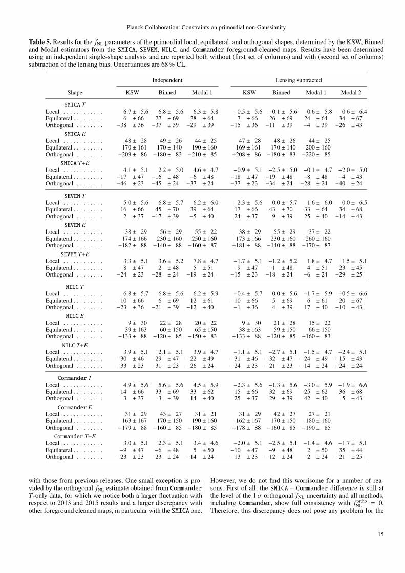
Planck Collaboration: Constraints on primordial non-Gaussianity
Table 5. Results for the fNL parameters of the primordial local, equilateral, and orthogonal shapes, determined by the KSW, Binnedand Modal estimators from the SMICA, SEVEM, NILC, and Commander foreground-cleaned maps. Results have been determinedusing an independent single-shape analysis and are reported both without (first set of columns) and with (second set of columns)subtraction of the lensing bias. Uncertainties are 68 % CL.
Independent Lensing subtracted
Shape KSW Binned Modal 1 KSW Binned Modal 1 Modal 2
SMICA TLocal . . . . . . . . . . . . 6.7 ± 5.6 6.8 ± 5.6 6.3 ± 5.8 −0.5 ± 5.6 −0.1 ± 5.6 −0.6 ± 5.8 −0.6 ± 6.4Equilateral . . . . . . . . . 6 ± 66 27 ± 69 28 ± 64 7 ± 66 26 ± 69 24 ± 64 34 ± 67Orthogonal . . . . . . . . −38 ± 36 −37 ± 39 −29 ± 39 −15 ± 36 −11 ± 39 −4 ± 39 −26 ± 43
SMICA ELocal . . . . . . . . . . . . 48 ± 28 49 ± 26 44 ± 25 47 ± 28 48 ± 26 44 ± 25Equilateral . . . . . . . . . 170 ± 161 170 ± 140 190 ± 160 169 ± 161 170 ± 140 200 ± 160Orthogonal . . . . . . . . −209 ± 86 −180 ± 83 −210 ± 85 −208 ± 86 −180 ± 83 −220 ± 85
SMICA T+ELocal . . . . . . . . . . . . 4.1 ± 5.1 2.2 ± 5.0 4.6 ± 4.7 −0.9 ± 5.1 −2.5 ± 5.0 −0.1 ± 4.7 −2.0 ± 5.0Equilateral . . . . . . . . . −17 ± 47 −16 ± 48 −6 ± 48 −18 ± 47 −19 ± 48 −8 ± 48 −4 ± 43Orthogonal . . . . . . . . −46 ± 23 −45 ± 24 −37 ± 24 −37 ± 23 −34 ± 24 −28 ± 24 −40 ± 24
SEVEM TLocal . . . . . . . . . . . . 5.0 ± 5.6 6.8 ± 5.7 6.2 ± 6.0 −2.3 ± 5.6 0.0 ± 5.7 −1.6 ± 6.0 0.0 ± 6.5Equilateral . . . . . . . . . 16 ± 66 45 ± 70 39 ± 64 17 ± 66 43 ± 70 33 ± 64 34 ± 68Orthogonal . . . . . . . . 2 ± 37 −17 ± 39 −5 ± 40 24 ± 37 9 ± 39 25 ± 40 −14 ± 43
SEVEM ELocal . . . . . . . . . . . . 38 ± 29 56 ± 29 55 ± 22 38 ± 29 55 ± 29 37 ± 22Equilateral . . . . . . . . . 174 ± 166 230 ± 160 250 ± 160 173 ± 166 230 ± 160 260 ± 160Orthogonal . . . . . . . . −182 ± 88 −140 ± 88 −160 ± 87 −181 ± 88 −140 ± 88 −170 ± 87
SEVEM T+ELocal . . . . . . . . . . . . 3.3 ± 5.1 3.6 ± 5.2 7.8 ± 4.7 −1.7 ± 5.1 −1.2 ± 5.2 1.8 ± 4.7 1.5 ± 5.1Equilateral . . . . . . . . . −8 ± 47 2 ± 48 5 ± 51 −9 ± 47 −1 ± 48 4 ± 51 23 ± 45Orthogonal . . . . . . . . −24 ± 23 −28 ± 24 −19 ± 24 −15 ± 23 −18 ± 24 −6 ± 24 −29 ± 25
NILC TLocal . . . . . . . . . . . . 6.8 ± 5.7 6.8 ± 5.6 6.2 ± 5.9 −0.4 ± 5.7 0.0 ± 5.6 −1.7 ± 5.9 −0.5 ± 6.6Equilateral . . . . . . . . . −10 ± 66 6 ± 69 12 ± 61 −10 ± 66 5 ± 69 6 ± 61 20 ± 67Orthogonal . . . . . . . . −23 ± 36 −21 ± 39 −12 ± 40 −1 ± 36 4 ± 39 17 ± 40 −10 ± 43
NILC ELocal . . . . . . . . . . . . 9 ± 30 22 ± 28 20 ± 22 9 ± 30 21 ± 28 15 ± 22Equilateral . . . . . . . . . 39 ± 163 60 ± 150 65 ± 150 38 ± 163 59 ± 150 66 ± 150Orthogonal . . . . . . . . −133 ± 88 −120 ± 85 −150 ± 83 −133 ± 88 −120 ± 85 −160 ± 83
NILC T+ELocal . . . . . . . . . . . . 3.9 ± 5.1 2.1 ± 5.1 3.9 ± 4.7 −1.1 ± 5.1 −2.7 ± 5.1 −1.5 ± 4.7 −2.4 ± 5.1Equilateral . . . . . . . . . −30 ± 46 −29 ± 47 −22 ± 49 −31 ± 46 −32 ± 47 −24 ± 49 −15 ± 43Orthogonal . . . . . . . . −33 ± 23 −31 ± 23 −26 ± 24 −24 ± 23 −21 ± 23 −14 ± 24 −24 ± 24
Commander TLocal . . . . . . . . . . . . 4.9 ± 5.6 5.6 ± 5.6 4.5 ± 5.9 −2.3 ± 5.6 −1.3 ± 5.6 −3.0 ± 5.9 −1.9 ± 6.6Equilateral . . . . . . . . . 14 ± 66 33 ± 69 33 ± 62 15 ± 66 32 ± 69 25 ± 62 36 ± 68Orthogonal . . . . . . . . 3 ± 37 3 ± 39 14 ± 40 25 ± 37 29 ± 39 42 ± 40 5 ± 43
Commander ELocal . . . . . . . . . . . . 31 ± 29 43 ± 27 31 ± 21 31 ± 29 42 ± 27 27 ± 21Equilateral . . . . . . . . . 163 ± 167 170 ± 150 190 ± 160 162 ± 167 170 ± 150 180 ± 160Orthogonal . . . . . . . . −179 ± 88 −160 ± 85 −180 ± 85 −178 ± 88 −160 ± 85 −190 ± 85Commander T+E
Local . . . . . . . . . . . . 3.0 ± 5.1 2.3 ± 5.1 3.4 ± 4.6 −2.0 ± 5.1 −2.5 ± 5.1 −1.4 ± 4.6 −1.7 ± 5.1Equilateral . . . . . . . . . −9 ± 47 −6 ± 48 5 ± 50 −10 ± 47 −9 ± 48 2 ± 50 35 ± 44Orthogonal . . . . . . . . −23 ± 23 −23 ± 24 −14 ± 24 −13 ± 23 −12 ± 24 −2 ± 24 −21 ± 25
with those from previous releases. One small exception is pro-vided by the orthogonal fNL estimate obtained from CommanderT-only data, for which we notice both a larger fluctuation withrespect to 2013 and 2015 results and a larger discrepancy withother foreground cleaned maps, in particular with the SMICA one.
However, we do not find this worrisome for a number of rea-sons. First of all, the SMICA – Commander difference is still atthe level of the 1σ orthogonal fNL uncertainty and all methods,including Commander, show full consistency with f ortho
NL = 0.Therefore, this discrepancy does not pose any problem for the
15

Planck Collaboration: Constraints on primordial non-Gaussianity
TTT
71.6%TTE
1.2%TET 1.9%TEE 4.6%
ETT
17.3%
ETE
0.6%
EET
1.0%
EEE
1.8%
Local
TTT
38.1%
TTE
10.5%
TET
9.1%
TEE
8.4%
ETT 15.7%
ETE
4.3%
EET
7.2%
EEE
6.8%
Equilateral
TTT
32.6%
TTE
8.2%
TET
13.9%
TEE
3.8%
ETT 28.9%
ETE
2.5%
EET
4.9%
EEE
5.3%
Orthogonal
Fig. 1. Weights of each polarization configuration going into the total value of fNL for, from left to right, local, equilateral, andorthogonal shapes. Note that since we impose `1 ≤ `2 ≤ `3, there is a difference between, e.g., TEE (smallest ` is temperature) andEET (largest ` is temperature).
Table 6. Results for the fNL parameters of the primordial local,equilateral, and orthogonal shapes, determined by the KSW es-timator from the SMICA foreground-cleaned map. Both indepen-dent single-shape results and results with the lensing bias sub-tracted are reported; uncertainties are 68 % CL. The differencebetween this table and the corresponding values in the previoustable is that here the equilateral and orthogonal shapes have beenanalysed jointly.
Shape Independent Lensing subtracted
SMICA TLocal . . . . . . . . . 6.7 ± 5.6 −0.5 ± 5.6Equilateral . . . . . . 4 ± 67 5 ± 67Orthogonal . . . . . −38 ± 37 −15 ± 37
SMICA T+ELocal . . . . . . . . . 4.1 ± 5.1 −0.9 ± 5.1Equilateral . . . . . . −25 ± 47 −26 ± 47Orthogonal . . . . . −47 ± 24 −38 ± 24
theoretical interpretation of the result. Moreover, this fluctuationcompletely goes away when accounting for polarization data, thereliability of which has become significantly higher with respectto our previous analysis (see Sect. 6 for details). Finally, the dis-crepancy is for a very specific shape and it is entirely driven bythe already-noted fluctuation in the Commander orthogonal re-sult with respect to 2013 and 2015. The other methods remainstable, in particular SMICA, which we take as the map of choicefor our final results. The observed fluctuation in orthogonal fNLfrom Commander can likely be explained by the unavailabilityof “detset” (i.e., detector-subset) maps for this release, whichconstituted in the past a useful input for improving the accuracyof the Commander map. It is, however, important to stress thatCommander itself shows excellent agreement with other meth-ods, when measuring fNL for all other shapes and also when cor-relating the bispectrum modes and bins in a model-independentfashion, both in temperature and polarization (again see Sect. 6for a complete discussion of these tests).
Comparing the uncertainties in Table 5 to those in the cor-responding table in the 2015 analysis paper (PCNG15), and fo-cussing on the ones for the local shape, since those are mostsensitive to low-` modes, we see the following: for T-only data
the errors are approximately equal on average, slightly better forKSW, and slightly worse for the other three estimators. A pos-sible explanation for the slightly larger errors could be the factthat the realism of the simulations has improved from FFP8 usedin 2015 to FFP10 used here. So the errors in 2015 might actu-ally have been slightly underestimated. However, the differencesare small enough that they could just be random fluctuations, es-pecially given that not all estimators show the same effect. ForE-only data we see a clear improvement of the errors for all es-timators. That is as expected, since we are now including all theadditional polarization modes with 4 ≤ ` < 40 in the analy-sis, and the local shape is quite sensitive to these low-` modes.Finally, for the full T+E analysis, we see that all errors haveremained the same, to within fluctuations of around a few per-cent, at most. So one might wonder why the improvement inthe E-only analysis has not translated into a corresponding im-provement in the T+E analysis. The answer is relatively simple:the EEE-bispectra only have a very small contribution to the fi-nal T+E analysis, as shown in Fig. 1. This figure also explainswhy the errors for the equilateral and orthogonal shapes improvemore when going from T-only to the full T+E analysis than theerrors for the local shape.
In conclusion, our current results show no evidence for non-Gaussianity of the local, equilateral, or orthogonal type and arein very good agreement with the previous 2013 and 2015 anal-yses. We also show in Sect. 6 that the overall robustness andinternal consistency of the polarization data set has significantlyimproved, as far as primordial non-Gaussian measurements areconcerned.
5.2. Further bispectrum shapes
5.2.1. Isocurvature non-Gaussianity
In this section we present a study of the isocurvature NG in thePlanck 2018 SMICAmap using the Binned bispectrum estimator.This analysis is complementary to the one based on the powerspectrum presented in Planck Collaboration X (2018). The un-derlying modelling approach was discussed in Sect. 2.3, and asexplained there, we only investigate isocurvature NG of the lo-cal type, and in addition always consider the adiabatic modetogether with only one isocurvature mode, i.e., we considerseparately CDM-density, neutrino-density, and neutrino-velocity
16

Planck Collaboration: Constraints on primordial non-Gaussianity
Table 7. Results for fNL for local isocurvature NG determined from the SMICA Planck 2018 map with the Binned bispectrumestimator. In each case the adiabatic mode is considered together with one isocurvature mode (either cold-dark-matter, neutrino-density, or neutrino-velocity isocurvature). As explained in the text this gives six different fNL parameters, indicated by the differentcombinations of the adiabatic (a) and isocurvature (i) modes. Results are shown for both an independent and a fully joint analysis,for T-only, E-only, and full T+E data. In all cases the lensing bias has been subtracted.
Independent Joint
Shape Cold dark matter Neutrino density Neutrino velocity Cold dark matter Neutrino density Neutrino velocity
T a,aa . . . . . . −0.1 ± 5.6 −0.1 ± 5.6 −0.1 ± 5.6 15 ± 16 −15 ± 54 −29 ± 49T a,ai . . . . . . −3 ± 11 −6 ± 16 27 ± 29 −30 ± 31 87 ± 220 310 ± 360T a,ii . . . . . . . 440 ± 950 −150 ± 290 480 ± 360 11000 ± 8500 −1800 ± 4500 −1100 ± 3800T i,aa . . . . . . 33 ± 53 0.3 ± 9.2 −0.1 ± 4.9 95 ± 120 46 ± 110 −27 ± 49T i,ai . . . . . . . 28 ± 67 −9 ± 23 14 ± 21 −1300 ± 1000 −32 ± 670 98 ± 170T i,ii . . . . . . . 110 ± 280 −130 ± 250 270 ± 230 2500 ± 2000 −140 ± 2600 −1000 ± 1400
E a,aa . . . . . . 48 ± 26 48 ± 26 48 ± 26 25 ± 42 −60 ± 120 43 ± 130E a,ai . . . . . . 140 ± 91 170 ± 98 72 ± 51 28 ± 150 330 ± 590 280 ± 370E a,ii . . . . . . . 100 ± 2500 2000 ± 1500 310 ± 460 −8100 ± 4400 −9400 ± 5500 −6100 ± 2800E i,aa . . . . . . 110 ± 77 75 ± 34 31 ± 21 43 ± 140 90 ± 170 −94 ± 120E i,ai . . . . . . . 330 ± 180 210 ± 100 43 ± 35 830 ± 580 500 ± 890 460 ± 360E i,ii . . . . . . . 1800 ± 1200 1900 ± 1100 170 ± 230 −1400 ± 2300 −1300 ± 4800 −380 ± 1000
T+E a,aa . . . . −2.5 ± 5.0 −2.5 ± 5.0 −2.5 ± 5.0 4 ± 10 −53 ± 28 2 ± 26T+E a,ai . . . . −10 ± 10 −14 ± 14 −1 ± 21 −14 ± 21 160 ± 110 250 ± 110T+E a,ii . . . . . −450 ± 520 −350 ± 260 −56 ± 210 −3100 ± 1500 −4100 ± 1600 −2100 ± 920T+E i,aa . . . . 20 ± 28 −0.5 ± 8.0 −3.5 ± 4.2 96 ± 52 44 ± 49 −37 ± 26T+E i,ai . . . . . −32 ± 46 −18 ± 20 −7 ± 14 190 ± 180 350 ± 240 23 ± 77T+E i,ii . . . . . −290 ± 210 −340 ± 210 −51 ± 110 −640 ± 400 −2000 ± 990 38 ± 300
TTT
26.9%
TTE
22.7%
TET
23.2%
TEE
20.8%
ETT
1.2%
ETE
1.4%
EET
1.8%
EEE
2.1%
CDM a,ii
TTT
78.7%
TTE1.4%
TET1.9%
TEE
7.2%
ETT
7.5%
ETE
0.9%
EET
1.3%
EEE
1.2%
Neutrino density a,ii
TTT
16.9% TTE
1.3% TET
2.0% TEE3.0%
ETT
63.8%
ETE
1.4%
EET
2.3%
EEE
9.3%
Neutrino velocity a,ii
Fig. 2. Weights of each polarization configuration going into the total value of the a,ii mixed fNL parameter for, from left to right,CDM, neutrino-density, and neutrino-velocity isocurvature, in addition to the adiabatic mode. Note that since we impose `1 ≤ `2 ≤
`3, there is a difference between, e.g., TEE (where the smallest ` is temperature) and EET (where the largest ` is temperature).
Table 8. Similar to Table 7, except that we now assume that the adiabatic and isocurvature modes are completely uncorrelated.Hence there are only two fNL parameters in this case, a purely adiabatic one and a purely isocurvature one.
Independent Joint
Shape Cold dark matter Neutrino density Neutrino velocity Cold dark matter Neutrino density Neutrino velocity
T a,aa . . . . . . −0.1 ± 5.6 −0.1 ± 5.6 −0.1 ± 5.6 −0.6 ± 5.7 15 ± 13 −1.3 ± 5.8T i,ii . . . . . . . 110 ± 280 −130 ± 250 270 ± 230 120 ± 290 −710 ± 590 280 ± 240
E a,aa . . . . . . 48 ± 26 48 ± 26 48 ± 26 41 ± 27 33 ± 35 62 ± 35E i,ii . . . . . . . 1800 ± 1200 1900 ± 1100 170 ± 230 1400 ± 1200 1000 ± 1400 −200 ± 300
T+E a,aa . . . . −2.5 ± 5.0 −2.5 ± 5.0 −2.5 ± 5.0 −1.3 ± 5.1 11.4 ± 8.4 −1.9 ± 5.2T+E i,ii . . . . . −290 ± 210 −340 ± 210 −51 ± 110 −280 ± 210 −710 ± 360 −41 ± 120
17

Planck Collaboration: Constraints on primordial non-Gaussianity
isocurvature. In that case there are in general six different fNL pa-rameters: the purely adiabatic one (a,aa) from Sect. 5.1; a purelyisocurvature one (i,ii); and four mixed ones.
The results can be found in Table 7, both for an independentanalysis of the six parameters (i.e., assuming that only one ofthe six parameters is present) and for a fully joint analysis (i.e.,assuming that all six parameters are present, which is clearly thecorrect thing to do in the correlated framework described above).Note that the reason for the very differently sized errors is acombination of two effects. The first is a simple normalizationissue, due to switching from the more natural ζ and S variables(commonly used in the inflation literature) to Φadi = 3ζ/5 andΦiso = S/5, which are more commonly used in the CMB lit-erature.8 The second is that certain parameters depend more onthe high-` adiabatic modes (which are well-determined), whileothers are dominated by the much suppressed, and hence uncon-strained, high-` isocurvature modes. For example, for the jointCDM T+E case, when compensating for the normalization fac-tor, one would find the error for a,aa and a,ai to be around 10, andthe other four errors to be around 200 (see Langlois & van Tent2012, for further discussion of these effects).
As in our analysis of the 2015 Planck data (PCNG15), wesee no clear sign of any isocurvature NG. There are a few val-ues that deviate from zero by up to about 2.5σ, but such a smalldeviation cannot be considered a detection, given the large num-ber of tests and the fact that the deviations are not consistentbetween T-only and T+E data. For example, looking at the 300Gaussian simulations that were used to determine the linear cor-rection and the uncertainties, we find that 84 of them have atleast one > 2.5σ result in the two CDM columns of Table 7,while for neutrino density and neutrino velocity the numbers are62 and 80, respectively.
We see that many constraints are tightened considerablywhen including polarization, by up to the predicted factor ofabout 5–6 for the CDM a,ii, i,ai, and i,ii modes in the joint anal-ysis (e.g., −1300 ± 1000 for T only, decreasing to 190 ± 180for T+E in the CDM i,ai case). Focussing now on the indepen-dent results, where it is easier to understand their behaviour (asthings are not mixed together), we see that the uncertainties ofsome of the CDM and neutrino-velocity modes improve by afactor of about 2 when going from the T-only to the full T+Eanalysis (e.g., neutrino velocity i,ii changes from 270 ± 230 to−51 ± 110), while the improvements for the neutrino-densitymodes are much smaller, of the order of what we see for thepure adiabatic mode. This can be explained if we look at thecontribution of the various polarization modes to the total fNLparameters, as indicated in Fig. 2 for the a,ii modes (to givean example). While the diagram for the neutrino-density modevery much resembles the one for the pure adiabatic local casein Fig. 1, those for CDM and neutrino velocity are quite differ-ent and have a much larger contribution from polarization modes(but quite different between the two cases). Hence isocurvatureNG also provides a good test of the quality of the polarizationmaps, and a clear motivation for extending our analyses to in-clude polarization in addition to temperature.
Comparing the results in Table 7 to those of the correspond-ing table in our 2015 analysis (PCNG15) we see in the first placethat the T-only results are mostly very stable, generally shift-ing by much less than 1σ (e.g., joint neutrino velocity i,ii is−970 ± 1400 in 2015 versus −1000 ± 1400 now). Secondly, forthe E-only results we see that all the errors have significantly
8 Conversion factors to obtain results based on ζ and S are 6/5, 2/5,2/15, 18/5, 6/5, and 2/5, for the six modes, respectively.
decreased (e.g., taking again joint neutrino velocity i,ii, we had2200 ± 1600 in 2015 versus −380 ± 1000 now), in line with thefact that we are now using the additional 4 ≤ ` < 40 E modes.We also generally see larger changes in the central values, withseveral shifts of 1σ or larger; nevertheless, the results are con-sistent with zero. Because we have added new polarization datato the analysis compared to 2015, and the quality of the polariza-tion data has improved overall, these larger shifts are not unex-pected. Finally, looking at the full T+E analysis, we see that thecentral values shift a bit more than for T only, but remain con-sistent with zero. For CDM and neutrino density the errors aremarginally larger than in 2015, similarly to what we see with theBinned estimator for the local adiabatic shape (see Sect. 5.1).As shown in Fig. 2, both of these depend very little on low-`polarization, and so are likely mostly driven by the marginal in-crease in the T-only errors. For the neutrino-velocity mode, onthe other hand, some of the errors do decrease (e.g., 480 ± 430in 2015 versus 38 ± 300 now for joint neutrino velocity i,ii).As seen in Fig. 2, this mode depends more strongly on the ETTcombination, which does involve low-` polarization.
In the results so far we looked at the most general case, hav-ing a possible correlation between the isocurvature and adiabaticmodes. However, if we assume that the adiabatic and the isocur-vature modes have a cross-power spectrum of zero and are com-pletely uncorrelated, then there are only two free fNL parameters,the a,aa and the i,ii ones. In Table 8 we present the results for thisuncorrelated case. The independent results are the same as in theprevious table and have been repeated for convenience. The sig-nificant increase in the T-only and T+E errors for the neutrinodensity case when going from the independent to the joint anal-ysis clearly illustrates the fact that its bispectrum template hasa large overlap with the adiabatic one, something that also ex-plains the similarity of Figs. 1 and 2 for that case. The CDM andneutrino-velocity modes, on the other hand, have templates thatare very different from the adiabatic one and their errors hardlyincrease (except for neutrino velocity for E-only data). Againthere is no evidence for any isocurvature NG: we do not con-sider the almost 2σ result for the neutrino-density isocurvaturemode in the T+E joint analysis to be significant, although it willbe interesting to keep an eye on this in future CMB experimentswith even better polarization measurements.
5.2.2. Running non-Gaussianity
In this section we present our analysis of the scale-dependentbispectrum shapes described in Sect. 2.4; we obtain these re-sults following the pipeline described in Sect. 3.1.2. In Figs. 3,4, and 5 we show the results, respectively, for the one-field lo-cal model (Eq. 8), the two-field local model (Eq. 10), and thegeometric-mean equilateral model, where f ∗NL is parametrizedas in Eq. (31). Here we present results for both the SMICA andCommander temperature maps. Since the E-mode polarizationmaps are not expected to significantly improve the constraints onnNG, while requiring a significant growth in the computationalcost of the estimation pipeline, we do not include polarizationin this particular analysis. We show the PDF inferred from allthree of the methodologies described. Each point is derived froma KSW estimate of the amplitude for the corresponding scale-dependent template with the given running. The KSW pipelineand the map processing steps are the same as applied to the es-timation of the local, equilateral, and orthogonal shapes. We in-clude in this analysis the multipole range from 2 to 2000 and theresults are corrected for the lensing bias. All curves in Figs. 3–5are normalized to integrate to one. We consider possible values
18

Planck Collaboration: Constraints on primordial non-Gaussianity
10 5 0 5 10nNG
PD
F
P(nNG), π= c
P(nNG), π=√
det(I)L(nNG)
10 5 0 5 10nNG
PD
F
P(nNG), π= c
P(nNG), π=√
det(I)L(nNG)
Fig. 3. PDF of the running parameter nNG for the one-field localmodel. Top: SMICAmap. Bottom: Commandermap. Blue squaresgive the marginalized posterior assuming a constant prior, greencircles are the posterior assuming a Jeffreys prior, and red trian-gles are the profiled Likelihood.
of the running in the interval nNG = [−10, 10]. This interval istwo orders of magnitude wider than the theoretical expectationof the models, which are valid in the regime of mild scale depen-dence, i.e., nNG ≈ 0.1.
The effects of the choice of prior are very obvious: if weadopt a constant prior (blue squares) we can always identify apeak in the distribution and define proper constraints; however,this is not the case for the other priors. If we implement an un-informative prior (green circles), the shape of the distributionbecomes complex, showing multiple peaks or even divergingon the boundaries, making it impossible to define constraints.A similar behaviour appears in the profiled likelihood approach(red triangles; see Eq. 36). We used the likelihood to also per-form a likelihood ratio test between its maximum value and thevalue for nNG = 0. Notice that in the case of zero running, thesemodels reduce to the usual local or equilateral shapes. We as-sume an acceptance threshold of α = 0.01 As expected, we donot find any evidence in favour of scale dependent models.
10 5 0 5 10nNG
PD
F
P(nNG), π= c
P(nNG), π=√
det(I)L(nNG)
10 5 0 5 10nNG
PD
F
P(nNG), π= c
P(nNG), π=√
det(I)L(nNG)
Fig. 4. PDF of the running parameter nNG for the two-field localmodel. Top: SMICAmap. Bottom: Commandermap. Blue squaresgive the marginalized posterior assuming a constant prior, greencircles are the posterior assuming a Jeffreys prior, and red trian-gles are the profiled Likelihood.
5.2.3. Resonance and axion monodromy
Now we present results from the Modal 2 and from an adaptedKSW-type estimator for the broad class of resonance-type mod-els. These models can be characterized by a bispectrum tem-plate having logarithmic oscillations with a scale, as introducedin Sect. 2.5.1. For the Modal 2 analysis we examine templateswith frequency in the range 0 < ω ≤ 50 and with a range of pos-sible cross-sectional behaviour covering constant, flat, local, andequilateral type templates to span a broader range of possiblemodels. The raw results have been maximized over phase andare presented in Fig. 6 for the four component-separation meth-ods. Since the errors grow with frequency due to increasing sup-pression by the both transfer functions and projection effects, weonly plot the raw significance. The results are consistent acrosscomponent-separation methods and are comparable with thosepreviously presented in PCNG15, but with slight reductions insignificance. Since we are surveying a large range of frequen-cies, we must correct our results for the “look-elsewhere” effect
19

Planck Collaboration: Constraints on primordial non-Gaussianity
10 5 0 5 10nNG
PD
F
P(nNG), π= c
P(nNG), π=√
det(I)L(nNG)
10 5 0 5 10nNG
PD
F
P(nNG), π= c
P(nNG), π=√
det(I)L(nNG)
Fig. 5. PDF of the running parameter nNG for the geometricmean equilateral parametrization. Top: SMICA map. Bottom:Commander map. Blue squares give the marginalized posteriorassuming a constant prior, green circles are the posterior assum-ing a Jeffreys prior, and red triangles are the profiled Likelihood.
to asses their true significance. This is done using the optimalmethods first proposed in Fergusson et al. (2015), which assessthe true significance of both single peaks and also clusters ofmultiple peaks (which may indicate a model in this class butwith a waveform that only partially correlates with the templatesused). The results are presented in Table 9, with the largest look-elsewhere-corrected result being for the equilateral cross-sectionwith around 2σ for a single peak. This is not on its own signif-icant, but may warrant further investigation with more realisticexact templates near this frequency.
5.2.4. Scale-dependent oscillatory features
In this section we show the broad range of oscillatory modelssourced through features in the inflationary potential or soundspeed, described in Sect. 2.5.2, which can be described by a sinu-soid multiplied by either a cross-sectional template or a scalingfunction. The results are plotted after maximization over phasein Figs. 7 and 8 with look-elsewhere-adjusted results presented
in Table 10. Here all results are consistent with Gaussianity forall models in this class.
5.2.5. High-frequency feature and resonant-model estimator
As in PCNG15, we have extended the frequency range of theconstant feature model and the constant resonance model witha second set of estimators. The constant feature bispectrum inEq. (15) is separable and thus allows for the construction of aKSW estimator (Munchmeyer et al. 2014) for direct bispectrumestimation at any given frequency. We use this method to probefrequencies up to ω = 3000. In the overlapping frequency rangewe also confirmed that the results are compatible with those ofthe Modal pipeline. The results are shown in the upper two pan-els of Fig. 9. Due to the computational demands of this estimatorwe have only analysed SMICA maps, since it was already shownin PCNG15 that all component-separations methods agree wellfor this estimator. No statistically significant peak is found, andthe distribution of peaks is consistent with the 2015 analysis. Thehighest peak is 2.9σ in T only and 3.5σ in T + E, compared tothe Gaussian expectation of 3.1(±0.3)σ.9
For the constant resonance model, we use the method ofMunchmeyer et al. (2015), which expands the logarithmic os-cillations in terms of separable linear oscillations. Here we use800 sine and cosine modes, to cover the frequency range 0 <ω < 1000. The results are shown in Fig. 7 (lower two panels) forSMICA data. The highest peak is 3.1σ for T only and 3.0σ forT + E, compared to the Gaussian expectation of 3.4σ ± 0.4σ.The Gaussian expectation was obtained from the covariance ma-trix of the estimators using the method of Meerburg et al. (2016).In summary we do not find evidence for non-Gaussianity in thehigh-frequency feature and resonance-model analysis.
We used the results obtained here to perform a joint powerand bispectrum analysis, which was presented in the accompa-nying paper Planck Collaboration X (2018) in a search for cor-related features. No evidence was found for such correlated fea-tures in either the power spectrum or the bispectrum.
5.2.6. Equilateral-type models and the effective field theoryof inflation
Many physically well-motivated inflationary models producenon-Gaussianity of the equilateral type. While the equilateraltemplate accurately approximates models in this class, it is nev-ertheless interesting to constrain the exact templates for two rea-sons. Firstly, while the equilateral template correlates well withthe true models, they are are only normalized in the equilaterallimit, which neglects the rest of configuration space and so isonly approximate. This is demonstrated by the fact that the un-certainties for the true templates differ by up to a factor of 2compared with the equilateral limit. Secondly, even small de-viations in correlation can result in much larger shifts in mea-surements, for example models that are 95 % correlated shouldproduce measurements that are on average 1/3σ apart. Here weconstrain the exact templates for all inflationary bispectra that fitinto the broad equilateral class; for details on these exact tem-plates we refer the reader to the paper PCNG15. The results forall models in this class are presented in Table 11 and are all be-
9 The Gaussian expectation is not zero because it is the average valueof the most significant fluctuation, maximized over the frequency andphase parameters of the shape. The expectation value of a single ampli-tude with a fixed frequency and phase is of course zero for a Gaussianmap.
20
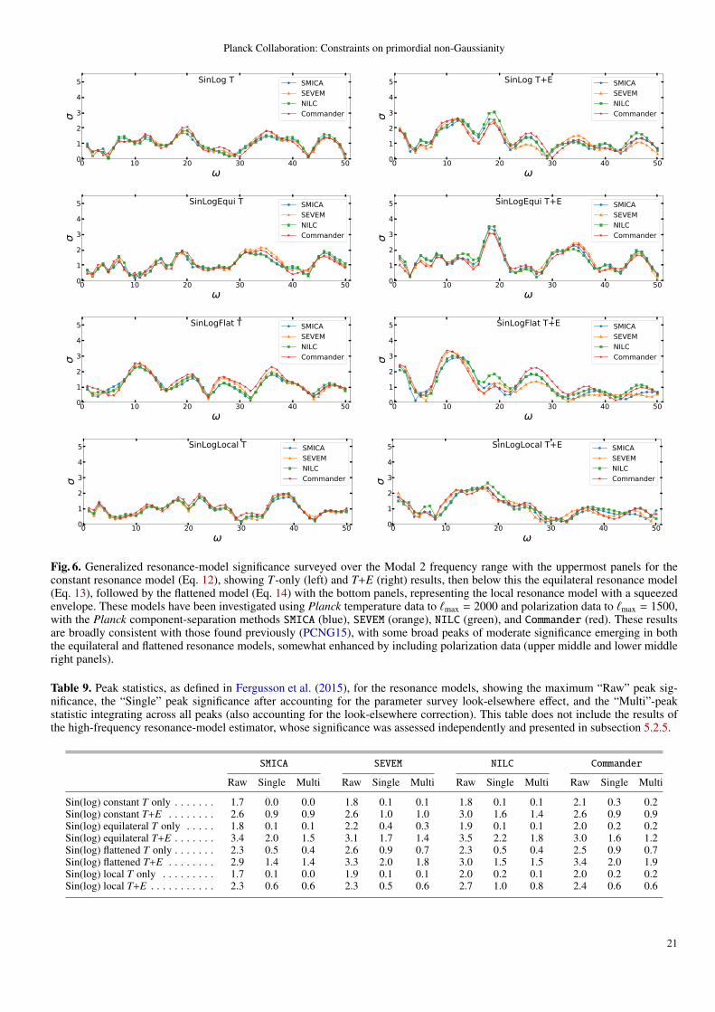
Planck Collaboration: Constraints on primordial non-Gaussianity
0 10 20 30 40 500
1
2
3
4
5 SinLog T SMICASEVEMNILCCommander
0 10 20 30 40 500
1
2
3
4
5 SinLog T+E SMICASEVEMNILCCommander
0 10 20 30 40 500
1
2
3
4
5 SinLogEqui T SMICASEVEMNILCCommander
0 10 20 30 40 500
1
2
3
4
5 SinLogEqui T+E SMICASEVEMNILCCommander
0 10 20 30 40 500
1
2
3
4
5 SinLogFlat T SMICASEVEMNILCCommander
0 10 20 30 40 500
1
2
3
4
5 SinLogFlat T+E SMICASEVEMNILCCommander
0 10 20 30 40 500
1
2
3
4
5 SinLogLocal T SMICASEVEMNILCCommander
0 10 20 30 40 500
1
2
3
4
5 SinLogLocal T+E SMICASEVEMNILCCommander
Fig. 6. Generalized resonance-model significance surveyed over the Modal 2 frequency range with the uppermost panels for theconstant resonance model (Eq. 12), showing T-only (left) and T+E (right) results, then below this the equilateral resonance model(Eq. 13), followed by the flattened model (Eq. 14) with the bottom panels, representing the local resonance model with a squeezedenvelope. These models have been investigated using Planck temperature data to `max = 2000 and polarization data to `max = 1500,with the Planck component-separation methods SMICA (blue), SEVEM (orange), NILC (green), and Commander (red). These resultsare broadly consistent with those found previously (PCNG15), with some broad peaks of moderate significance emerging in boththe equilateral and flattened resonance models, somewhat enhanced by including polarization data (upper middle and lower middleright panels).
Table 9. Peak statistics, as defined in Fergusson et al. (2015), for the resonance models, showing the maximum “Raw” peak sig-nificance, the “Single” peak significance after accounting for the parameter survey look-elsewhere effect, and the “Multi”-peakstatistic integrating across all peaks (also accounting for the look-elsewhere correction). This table does not include the results ofthe high-frequency resonance-model estimator, whose significance was assessed independently and presented in subsection 5.2.5.
SMICA SEVEM NILC Commander
Raw Single Multi Raw Single Multi Raw Single Multi Raw Single Multi
Sin(log) constant T only . . . . . . . 1.7 0.0 0.0 1.8 0.1 0.1 1.8 0.1 0.1 2.1 0.3 0.2Sin(log) constant T+E . . . . . . . . 2.6 0.9 0.9 2.6 1.0 1.0 3.0 1.6 1.4 2.6 0.9 0.9Sin(log) equilateral T only . . . . . 1.8 0.1 0.1 2.2 0.4 0.3 1.9 0.1 0.1 2.0 0.2 0.2Sin(log) equilateral T+E . . . . . . . 3.4 2.0 1.5 3.1 1.7 1.4 3.5 2.2 1.8 3.0 1.6 1.2Sin(log) flattened T only . . . . . . . 2.3 0.5 0.4 2.6 0.9 0.7 2.3 0.5 0.4 2.5 0.9 0.7Sin(log) flattened T+E . . . . . . . . 2.9 1.4 1.4 3.3 2.0 1.8 3.0 1.5 1.5 3.4 2.0 1.9Sin(log) local T only . . . . . . . . . 1.7 0.1 0.0 1.9 0.1 0.1 2.0 0.2 0.1 2.0 0.2 0.2Sin(log) local T+E . . . . . . . . . . . 2.3 0.6 0.6 2.3 0.5 0.6 2.7 1.0 0.8 2.4 0.6 0.6
21

Planck Collaboration: Constraints on primordial non-Gaussianity
0 50 100 150 200 250 300 3500
1
2
3
4
5 Feature T SMICASEVEMNILCCommander
0 50 100 150 200 250 300 3500
1
2
3
4
5 Feature T+E SMICASEVEMNILCCommander
0 50 100 150 200 250 300 3500
1
2
3
4
5 FeatEqui T SMICASEVEMNILCCommander
0 50 100 150 200 250 300 3500
1
2
3
4
5 FeatEqui T+E SMICASEVEMNILCCommander
0 50 100 150 200 250 300 3500
1
2
3
4
5 FeatFlat T SMICASEVEMNILCCommander
0 50 100 150 200 250 300 3500
1
2
3
4
5 FeatFlat T+E SMICASEVEMNILCCommander
Fig. 7. Generalized feature model significance surveyed over the Modal 2 frequency range 0 < ω < 350, after marginalizing over thephase φ. The top panels show results for the constant feature model (Eq. 15) with T only (left) and T+E (right), the middle panels forthe equilateral feature model (Eq. 18), and the bottom panels for the flattened feature model (Eq. 19). The same conventions applyas in Fig. 6. These feature model results generally have lower significance than obtained previously (PCNG15), with polarizationdata not tending to reinforce apparent peaks found using temperature data only.
0 50 100 150 200 250 300 3500
1
2
3
4
5 K2Cos T SMICASEVEMNILCCommander
0 50 100 150 200 250 300 3500
1
2
3
4
5 K2Cos T+E SMICASEVEMNILCCommander
0 50 100 150 200 250 300 3500
1
2
3
4
5 KSin T SMICASEVEMNILCCommander
0 50 100 150 200 250 300 3500
1
2
3
4
5 KSin T+E SMICASEVEMNILCCommander
Fig. 8. Top: Significance of single-field models for the potential feature case with a K2 cosωK scaling dependence (Eq. 16). Bottom:significance for rapidly varying sound speed with a K sinωK scaling (Eq. 17). Left panels are for T only and left panels are forT + E. These results have been marginalized over the envelope parameter α (determined by feature width and height) from α = 0to αω = 90. There appears to be no evidence for these very specific signatures in this frequency range when polarization data areincluded.
low 1σ, as expected due to their correlation with the equilateraltemplate, but with significant spread due to the small differencesin correlation between templates.
22

Planck Collaboration: Constraints on primordial non-Gaussianity
Table 10. Peak statistics, as defined in Fergusson et al. (2015), for the different feature models, showing the “Raw” peak maximumsignificance (for the given Modal 2 survey domain), the corrected significance of this “Single” maximum peak after accounting forthe parameter survey size (the look-elsewhere effect) and the “Multi”-peak statistic which integrates across the adjusted significanceof all peaks to determine consistency with Gaussianity. This table does not include the results of the high-frequency resonance-modelestimator, whose significance was assessed independently and presented in subsection 5.2.5.
SMICA SEVEM NILC Commander
Raw Single Multi Raw Single Multi Raw Single Multi Raw Single Multi
Features constant T only . . . . . . . 2.4 0.2 0.2 2.6 0.5 0.5 2.4 0.2 0.3 2.6 0.4 0.5Features constant T+E . . . . . . . . 2.5 0.3 0.3 2.7 0.6 0.7 2.8 0.8 1.2 2.6 0.4 0.5Features equilateral T only . . . . . 2.5 0.3 0.4 2.5 0.3 0.5 2.6 0.4 0.6 2.6 0.4 0.6Features equilateral T+E . . . . . . 2.5 0.3 0.3 2.5 0.3 0.3 3.0 1.1 1.1 2.4 0.2 0.2Features flattened T only . . . . . . . 2.7 0.6 0.8 2.8 0.7 1.0 2.6 0.5 0.6 2.9 0.9 0.9Features flattened T+E . . . . . . . . 2.4 0.2 0.4 2.7 0.6 0.9 2.7 0.6 0.7 2.5 0.3 0.5K2 cos features T only . . . . . . . . 2.0 0.0 0.0 2.0 0.0 0.0 2.0 0.0 0.0 2.1 0.0 0.0K2 cos features T+E . . . . . . . . . 1.7 0.0 0.0 2.1 0.0 0.0 1.6 0.0 0.0 1.5 0.0 0.0K sin features T only . . . . . . . . . 2.8 0.7 0.7 3.0 1.0 1.0 2.9 0.8 0.8 2.8 0.8 0.8K sin features T+E . . . . . . . . . . 2.3 0.1 0.1 2.6 0.4 0.4 2.7 0.5 0.6 2.3 0.1 0.1
Table 11. Constraints on models with equilateral-type NG covering the shapes predicted by the effective field theory of inflation,together with constraints on specific non-canonical inflation models, such as DBI inflation; see section 2 of PCNG13 for detailedexplanation of these specific models, with further implications discussed in Sect. 8.
SMICA SEVEM NILC Commander
Equilateral-type model A ± σA S/N A ± σA S/N A ± σA S/N A ± σA S/N
Constant T only . . . . . . . . . 31 ± 38 0.8 24 ± 38 0.6 15 ± 38 0.4 15 ± 38 0.4Constant T+E . . . . . . . . . . 21 ± 24 0.9 18 ± 25 0.7 7 ± 24 0.3 14 ± 25 0.6Equilateral T only . . . . . . . 34 ± 67 0.5 34 ± 68 0.5 20 ± 67 0.3 36 ± 68 0.5Equilateral T+E . . . . . . . . . −5 ± 43 −0.1 2 ± 45 0.1 −16 ± 43 −0.4 4 ± 44 0.1EFT shape 1 T only . . . . . . 43 ± 61 0.7 41 ± 63 0.6 26 ± 61 0.4 39 ± 62 0.6EFT shape 1 T+E . . . . . . . 8 ± 40 0.2 10 ± 41 0.2 −7 ± 40 −0.2 10 ± 41 0.3EFT shape 2 T only . . . . . . 51 ± 47 1.1 45 ± 48 1.0 33 ± 46 0.7 37 ± 47 0.8EFT shape 2 T+E . . . . . . . 28 ± 30 0.9 23 ± 31 0.8 11 ± 30 0.4 21 ± 31 0.7DBI inflation T only . . . . . . 46 ± 58 0.8 43 ± 60 0.7 29 ± 58 0.5 39 ± 59 0.7DBI inflation T+E . . . . . . . 14 ± 38 0.4 14 ± 39 0.4 −2 ± 38 −0.1 14 ± 39 0.4Ghost inflation T only . . . . . 6 ± 81 0.1 13 ± 83 0.2 −0 ± 81 −0.0 25 ± 82 0.3Ghost inflation T+E . . . . . . −48 ± 52 −0.9 −30 ± 54 −0.6 −50 ± 52 −1.0 −25 ± 53 −0.5Inverse decay T only . . . . . 38 ± 41 0.9 32 ± 42 0.8 21 ± 41 0.5 23 ± 42 0.5Inverse decay T+E . . . . . . 24 ± 27 0.9 19 ± 27 0.7 8 ± 26 0.3 17 ± 27 0.6
5.2.7. Models with excited initial states (non-Bunch-Daviesvacua)
Inflationary models that modify the initial vacuum for the in-flaton generally produce shapes in the flattened class, meaningthat they peak in triangle configurations with zero area. Thereis a wide variety of models of this type proposed in the litera-ture, which are described in detail in Sect. 2.6. For simplicitywe also include here the results for the warm inflation template,described in Sect. 2.2, since it exhibits similar behaviour onceprojected, despite the mechanism behind it being quite different.The results for this class are presented in Table 12. The mostsignificant measurement is for the NBD sin template, which pro-duces results around 2σ. However, it is important to note thatthis result involves a marginalization over a frequency type pa-rameter so there is a look-elsewhere effect that has not yet beentaken into account. Because of this we expect the true signifi-cance will be lower, so we can safely claim that our results areconsistent with Gaussianity, while noting that it may be inter-esting to revisit oscillatory NBD templates, like the NBD sinmodel, using future data sets.
5.2.8. Direction-dependent primordial non-Gaussianity
Here we present results for inflationary models where gaugefields induce a direction dependance to a “local” bispectrum, asdescribed in Sect. 2.7. Results for the L = 1 and L = 2 templatesare presented in Table 13 from the Modal 2 pipeline. Due to thecomplicated behaviour in the squeezed limit, the convergence forthese models is lower than for some others, but the Modal corre-lation remains above 93 % so a perfect estimator may see shiftsof order 0.5σ. The largest result is 1.9σ for L = 1 and SMICA,but this is not seen consistently across all component-separationmethods so cannot be considered robust. We can then concludethat our results are consistent with Gaussianity.
5.2.9. Parity-violating tensor non-Gaussianity motivated bypseudo-scalars
In this section, we report constraints on the tensor nonlinear-ity parameter f tens
NL (Eq. 22) obtained from temperature and E-mode polarization maps. As in our 2015 analysis, we exam-ine even and odd `1 + `2 + `3 multipole domains, employingthe original parity-even Modal estimator, f even
NL (Fergusson et al.
23
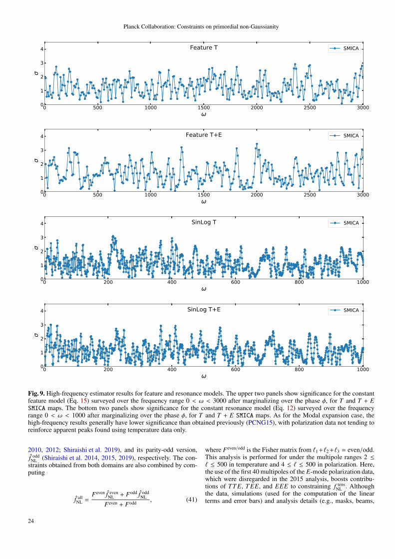
Planck Collaboration: Constraints on primordial non-Gaussianity
0 500 1000 1500 2000 2500 30000
1
2
3
4 Feature T SMICA
0 500 1000 1500 2000 2500 30000
1
2
3
4 Feature T+E SMICA
0 200 400 600 800 10000
1
2
3
4 SinLog T SMICA
0 200 400 600 800 10000
1
2
3
4 SinLog T+E SMICA
Fig. 9. High-frequency estimator results for feature and resonance models. The upper two panels show significance for the constantfeature model (Eq. 15) surveyed over the frequency range 0 < ω < 3000 after marginalizing over the phase φ, for T and T + ESMICA maps. The bottom two panels show significance for the constant resonance model (Eq. 12) surveyed over the frequencyrange 0 < ω < 1000 after marginalizing over the phase φ, for T and T + E SMICA maps. As for the Modal expansion case, thehigh-frequency results generally have lower significance than obtained previously (PCNG15), with polarization data not tending toreinforce apparent peaks found using temperature data only.
2010, 2012; Shiraishi et al. 2019), and its parity-odd version,f oddNL (Shiraishi et al. 2014, 2015, 2019), respectively. The con-
straints obtained from both domains are also combined by com-puting
f allNL =
Feven f evenNL + Fodd f odd
NL
Feven + Fodd , (41)
where Feven/odd is the Fisher matrix from `1 +`2 +`3 = even/odd.This analysis is performed for under the multipole ranges 2 ≤` ≤ 500 in temperature and 4 ≤ ` ≤ 500 in polarization. Here,the use of the first 40 multipoles of the E-mode polarization data,which were disregarded in the 2015 analysis, boosts contribu-tions of TT E, T EE, and EEE to constraining f tens
NL . Althoughthe data, simulations (used for the computation of the linearterms and error bars) and analysis details (e.g., masks, beams,
24

Planck Collaboration: Constraints on primordial non-Gaussianity
Table 12. Constraints on models with excited initial states (non-Bunch-Davies models), as well as warm inflation; see Sect. 2for further explanation and the labelling of these classes of NBD models. Note that the NBD, NBD1, and NBD2 models containfree parameters, so here we quote the maximum significance found over the entire parameter range. Note that the location of themaximum for T and T+E can occur for different parameter values for the model, and so the results with and without polarizationcannot be directly compared; however, the model parameters are held fixed across different component-separation methods.
SMICA SEVEM NILC Commander
Flattened-type model A ± σA S/N A ± σA S/N A ± σA S/N A ± σA S/N
Flat model T only . . . . . . . . . . . . . . . . . 56 ± 72 0.8 37 ± 72 0.5 23 ± 71 0.3 7 ± 72 0.1Flat model T+E . . . . . . . . . . . . . . . . . . 60 ± 43 1.4 44 ± 44 1.0 29 ± 43 0.7 33 ± 44 0.8Non-Bunch-Davies T only . . . . . . . . . . 13 ± 89 0.1 6 ± 90 0.1 −25 ± 88 −0.3 −17 ± 90 −0.2Non-Bunch-Davies T+E . . . . . . . . . . . 60 ± 54 1.1 38 ± 56 0.7 32 ± 53 0.6 44 ± 55 0.8NBD sin T only . . . . . . . . . . . . . . . . . . −630 ± 445 −1.4 −673 ± 450 −1.5 −629 ± 444 −1.4 −747 ± 445 −1.7NBD sin T+E . . . . . . . . . . . . . . . . . . . −496 ± 247 −2.0 −483 ± 255 −1.9 −547 ± 249 −2.2 −505 ± 253 −2.0NBD1 cos flattened T only . . . . . . . . . . 6 ± 21 0.3 8 ± 21 0.4 3 ± 21 0.1 5 ± 22 0.2NBD1 cos flattened T+E . . . . . . . . . . . 2 ± 15 0.1 6 ± 16 0.4 −7 ± 15 −0.5 1 ± 16 0.0NBD2 cos squeezed T only . . . . . . . . . . 48 ± 167 0.3 41 ± 170 0.2 −14 ± 166 −0.1 11 ± 170 0.1NBD2 cos squeezed T+E . . . . . . . . . . . −5.0 ± 6.0 −0.8 −6.5 ± 6.2 −1.1 −6.7 ± 6.0 −1.1 −5.6 ± 6.0 −0.9NBD1 sin flattened T only . . . . . . . . . . −22 ± 26 −0.8 −33 ± 26 −1.3 −27 ± 27 −1.0 −38 ± 27 −1.4NBD1 sin flattened T+E . . . . . . . . . . . −14 ± 20 −0.7 −22 ± 20 −1.1 −19 ± 20 −1.0 −24 ± 20 −1.2NBD2 sin squeezed T only . . . . . . . . . . −0.5 ± 0.6 −0.7 −0.3 ± 0.5 −0.6 −2.9 ± 2.6 −1.1 −0.8 ± 0.7 −1.1NBD2 sin squeezed T+E . . . . . . . . . . . −0.3 ± 0.4 −0.7 −0.2 ± 0.4 −0.5 −0.4 ± 0.4 −0.9 −0.4 ± 0.4 −1.0NBD3 non-canonical (×1000) T only . . . −4.4 ± 7.8 −0.6 −5.6 ± 7.9 −0.7 −4.6 ± 8.0 −0.6 −5.5 ± 7.9 −0.7NBD3 non-canonical (×1000) T+E . . . . −6.4 ± 5.8 −1.1 −7.5 ± 5.9 −1.3 −5.8 ± 5.9 −1.0 −6.2 ± 5.9 −1.0WarmS inflation T only . . . . . . . . . . . . −39 ± 44 −0.9 −35 ± 44 −0.8 −34 ± 44 −0.8 −18 ± 44 −0.4WarmS inflation T+E . . . . . . . . . . . . . . −48 ± 27 −1.8 −37 ± 28 −1.3 −41 ± 28 −1.5 −27 ± 28 −1.0
Table 13. Direction-dependent NG results for both the L = 1 and L = 2 models from the Modal 2 pipeline.
SMICA SEVEM NILC Commander
Equilateral-type model A ± σA S/N A ± σA S/N A ± σA S/N A ± σA S/N
L = 1Modal 2 T only . . . . . . . . . −51 ± 51 −1.0 −40 ± 51 −0.8 −41 ± 52 −0.8 −18 ± 52 −0.3Modal 2 T+E . . . . . . . . . . −57 ± 30 −1.9 −42 ± 31 −1.4 −42 ± 30 −1.4 −31 ± 31 −1.0
L = 2Modal 2 T only . . . . . . . . . 1.2 ± 3.0 0.4 1.7 ± 3.1 0.5 1.3 ± 3.1 0.4 0.5 ± 3.1 0.1Modal 2 T+E . . . . . . . . . . 0.9 ± 2.4 0.4 1.8 ± 2.4 0.7 −0.2 ± 2.4 −0.1 −0.2 ± 2.4 −0.1
and noise distributions) are somewhat different, other settingsfor the f tens
NL estimation are basically the same as in the 2015analysis (PCNG15).
The results from four different component-separated mapsare summarized in Table 14. We confirm there that the sizesof errors in the parity-odd T+E analysis reduce to almost thesame level as the parity-even counterparts. This is because thelow-` signal of TT E, which dominates the signal-to-noise ratiofrom `1 + `2 + `3 = odd (Shiraishi et al. 2013b), is now takeninto account. Although the errors for the parity-even case are aslarge as the 2015 ones, owing to the sensitivity improvement ofthe parity-odd part, the whole-domain constraints become morestringent.
Regardless of some updates, we find no > 2σ signal, whichis consistent with the conclusion of the 2015 analysis. This indi-cates no parity violation in the primordial Universe and accord-ingly gives constraints on some axion inflationary models (seeSect. 8.3).
5.3. Bispectrum reconstruction
5.3.1. Modal bispectrum reconstruction
The Modal bispectrum estimator filters the Planck foreground-removed CMB maps, i.e., SMICA, SEVEM, NILC, and Commander,using nmax = 2001 polynomial modes to obtain model coef-ficients βn. This procedure is undertaken to obtain all auto-and cross-correlations between the temperature and polarizationcomponents TTT, TTE, TEE, and EEE. We can then use the βncoefficients with the polynomial modes to obtain a full 3D recon-struction of the Planck temperature and polarization bispectraand this is shown in Fig. 10. These bispectra are in close agree-ment with those published in the paper analysing the Planck2015 results (PCNG15) when comparison is made in the signal-dominated regime.
5.3.2. Binned bispectrum reconstruction
The Binned bispectrum estimator can also be used to study thebispectrum itself, in addition to determining the fNL amplitudesof specific templates, as in the previous sections. In particular wecan investigate if any non-Gaussianity beyond that of the explicitmodels tested can be found in the cleaned CMB maps. Since we
25

Planck Collaboration: Constraints on primordial non-Gaussianity
Table 14. Results for the tensor nonlinearity parameter f tensNL /102
obtained from the SMICA, SEVEM, NILC, and Commander tem-perature and polarization maps. The central values and the er-rors (68 % CL) extracted from `1 + `2 + `3 = even (“Even”),`1 + `2 + `3 = odd (“Odd”), and their whole domain (“All”) areseparately described. One can see that all T-only results are ingood agreement with both the Planck 2015 ones (PCNG15) andWMAP ones (Shiraishi et al. 2015).
Even Odd All
SMICAT . . . . . . . . . . . . 4 ± 17 100 ± 100 6 ± 16E . . . . . . . . . . . . 33 ± 67 −570 ± 720 29 ± 67T+E . . . . . . . . . . 11 ± 14 1 ± 18 8 ± 11
SEVEMT . . . . . . . . . . . . 4 ± 17 90 ± 100 6 ± 16E . . . . . . . . . . . . 75 ± 75 −790 ± 830 70 ± 75T+E . . . . . . . . . . 16 ± 14 2 ± 20 13 ± 12
NILCT . . . . . . . . . . . . 4 ± 17 90 ± 100 6 ± 16E . . . . . . . . . . . . −16 ± 81 −540 ± 820 −19 ± 80T+E . . . . . . . . . . 6 ± 14 3 ± 21 5 ± 11
CommanderT . . . . . . . . . . . . 5 ± 17 90 ± 100 6 ± 16E . . . . . . . . . . . . 21 ± 69 −1200 ± 700 13 ± 69T+E . . . . . . . . . . 10 ± 14 −2 ± 19 7 ± 11
want to detect specific bin-triplets standing out from the noise,we work with the linear-term-corrected signal-to-noise-ratio bis-pectrum. Except for the high-` bins, where a point-source signalis present, the bin-triplets are noise dominated. Instead of rebin-ning, we can use a Gaussian kernel to smooth the bispectrum,so that structure localized in harmonic space stands out from thenoise. In this process, we mask out a few bin-triplets that havenon-Gaussian noise (due to the fact that they contain very fewvalid `-triplets). We also have to take into account edge effectsfrom the non-trivial domain of definition of the bispectrum. Themethod has been described in PCNG15 and more extensively inBucher et al. (2016).
Slices of the smoothed binned signal-to-noise bispectrumBi1i2i3 , with a Gaussian smoothing of σbin = 2, are shown inFigs. 11 and 12. These are slices for the 20th and 40th `3-bin as a function of `1 and `2. For the cross-bispectra mixingT and E modes, we defined BT2E
i1i2i3≡ BTT E
i1i2i3+ BT ET
i1i2i3+ BETT
i1i2i3;
and BT E2i1i2i3
≡ BT EEi1i2i3
+ BET Ei1i2i3
+ BEETi1i2i3
, with corresponding vari-ances Var(BT2E) = Var(TT E) + Var(T ET ) + Var(ETT ) + 2Cov(TT E,T ET ) + 2 Cov(TT E, ETT ) + 2 Cov(T ET, ETT ),and similarly for Var(BT E2), where we have omitted the bin in-dices for clarity. The red and blue regions correspond to a sig-nificant NG, whereas grey areas in Figs. 11 and 12 show regionswhere the bispectrum is not defined. Results are shown for thefour component-separation methods SMICA, SEVEM, NILC, andCommander, and for TTT, T2E, TE2, and EEE. We also showthe TTT bispectra after we remove the best joint-fit unclusteredand clustered point-source contribution (see Table 4). In the toprow of Fig. 12, we can clearly see this significant point-sourcesignal at high `. The T2E and TE2 bispectra do not have any ob-vious signals standing out, but we see some stronger NG in theEEE combination. Removing the best joint-fit contribution fromall shapes (Tables 4 and 5) does not reduce this region (a casewe do not show). The main difference with the previous release
is the better qualitative agreement between the four component-separation methods in polarization, as was already the case fortemperature. Commander and SEVEM now show similar struc-tures as the NILC and SMICA bispectra, which have remainedquite stable.
In order to quantify the possible residual non-Gaussianity inthese smoothed bispectra, we focus on the minimum and maxi-mum of our bin-triplets. In the case of statistically independentGaussian numbers, we can calculate the probability distributionof the extreme value statistics. However, once we introduce cor-relations due to the smoothing with non-trivial boundary con-ditions, we do not have an analytical formula. We can insteadgenerate Monte Carlo simulations of Gaussian random numberswith the same boundary conditions, apply the smoothing as forthe data signal-to-noise bispectrum, and compute the p-valuesof the observed extremum statistics as the fraction of simula-tions having a more extreme extremum than our data. This re-quires many simulations to study the very unlikely events. In thecurrent analysis, 106 Monte Carlo simulations turn out to be suf-ficient and so we do not need to use the semi-analytical Ansatzintroduced in Bucher et al. (2016).
In Table 15, we report for the smoothing lengths σbin = 1, 2,and 3, the two-tailed p-value10 of the maximum and of the min-imum, defined as p = 2 min
[Prob(XMC ≤ Xdata),Prob(XMC ≥
Xdata)], where X is either the minimum or the maximum of the
distribution. As expected, we detect a highly significant depar-ture from Gaussian statistics in the maxima for TTT when we donot correct for the contribution from point sources, and the sig-nal stands out more when increasing the smoothing kernel size.When looking at the SEVEM data for σbin = 2 and 3, we find nosimulation with a higher maximum, but for all the other casesour analysis should be robust. Most bispectra seem to be com-patible with a simple Gaussian distribution, except for the EEEbispectrum in the region shown in Fig. 12, for multipole tripletsaround [900, 1300, 1800]. We also see some significantly highmaxima for the TTT bispectrum of SEVEM and Commander (evenafter correcting for point sources), located around [800, 1100,2000] (shown in Fig. 13). The origin of these signals clusteredin multipole space is not understood.
6. Validation of Planck results
Two important potential sources of systematic effects in fNL es-timation are foreground residuals (which can also be related tothe choice of mask) and an imperfect modelling of instrumen-tal noise, either of which can lead to miscalibration of the linearcorrection term in the estimator. In this section, we perform abattery of tests aimed at testing the impact of these systematics.We will typically choose only one of the the KSW, Binned, orModal pipelines for each of the tests described below. This ispossible because of their excellent and well-verified agreementon both data and simulations.
10 While a one-tailed p-value quantifies how likely it is for the max-ima (a similar description holds for the minima) of the Monte Carlosimulations to be higher than the maximum of the data, the two-tailedp-value also considers how likely it is for it to be lower than that ofthe data. This means that a maximum that is too low will yield a lowp-value too.
26
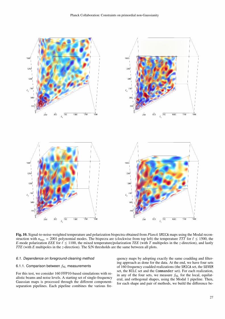
Planck Collaboration: Constraints on primordial non-Gaussianity
Fig. 10. Signal-to-noise-weighted temperature and polarization bispectra obtained from Planck SMICAmaps using the Modal recon-struction with nmax = 2001 polynomial modes. The bispecra are (clockwise from top left) the temperature TTT for ` ≤ 1500, theE-mode polarization EEE for ` ≤ 1100, the mixed temperature/polarization TEE (with T multipoles in the z-direction), and lastlyTTE (with E multipoles in the z-direction). The S/N thresholds are the same between all plots.
6.1. Dependence on foreground-cleaning method
6.1.1. Comparison between fNL measurements
For this test, we consider 160 FFP10-based simulations with re-alistic beams and noise levels. A starting set of single-frequencyGaussian maps is processed through the different component-separation pipelines. Each pipeline combines the various fre-
quency maps by adopting exactly the same coadding and filter-ing approach as done for the data. At the end, we have four setsof 160 frequency coadded realizations (the SMICA set, the SEVEMset, the NILC set and the Commander set). For each realization,in any of the four sets, we measure fNL for the local, equilat-eral, and orthogonal shapes, using the Modal 1 pipeline. Then,for each shape and pair of methods, we build the difference be-
27
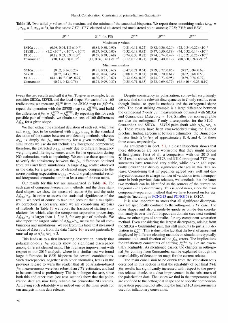
Planck Collaboration: Constraints on primordial non-Gaussianity
Table 15. Two-tailed p-values of the maxima and the minima of the smoothed bispectra. We report three smoothing scales (σbin =1, σbin = 2, σbin = 3), for five cases: TTT ; TTT cleaned of clustered and unclustered point sources; T2E; T E2; and EEE.
BTTT BTTT (no PS) BT2E BTE2 BEEE
Maximum p-valuesSMICA . . . . . (0.08, 0.04, 1.8 ×10⁻³) (0.84, 0.80, 0.95) (0.21, 0.11, 0.72) (0.82, 0.36, 0.20) (72, 0.34, 0.22) ×10−2
SEVEM . . . . . (1.2 ×10⁻⁴ , < 10−6, < 10−6) (0.27, 0.03, 0.03) (0.32, 0.18, 0.82) (0.37, 0.50, 0.89) (44, 0.32, 0.14) ×10−2
NILC . . . . . . (0.18, 0.03, 3.9 ×10⁻³) (0.59, 0.38, 0.68) (0.74, 0.33, 0.82) (0.94, 0.74, 0.49) (31, 0.21, 0.25) ×10−2
Commander . (70, 1.4, 0.3) ×10−3 (12, 0.66, 0.61) ×10−2 (0.12, 0.19, 0.71) (0.70, 0.40, 0.19) (88, 2.0, 0.92) ×10−2
Minimum p-valuesSMICA . . . . . (0.02, 0.14, 0.20) (0.25, 0.23, 0.62) (0.47, 0.21, 0.54) (0.59, 0.72, 0.86) (0.27, 0.94, 0.68)SEVEM . . . . . (0.32, 0.43, 0.98) (0.96, 0.84, 0.45) (0.08, 0.75, 0.81) (0.18, 0.70, 0.64) (0.62, 0.68, 0.53)NILC . . . . . . (8.1 ×10⁻³, 0.05, 0.27) (0.30, 0.21, 0.67) (0.32, 0.54, 0.93) (0.73, 0.73, 0.95) (0.89, 0.74, 0.72)Commander . (0.21, 0.42, 0.76) (0.74, 0.99, 0.37) (0.25, 0.71, 0.63) (0.73, 0.69, 0.77) (4.6 ×10⁻³, 0.25, 0.19)
tween the two results and call it ∆ fNL. To give an example, let usconsider SMICA, SEVEM, and the local shape. For each of the 160realizations, we measure f local
NL from the SMICA map (≡ f SMICANL ),repeat the operation with the SEVEM map (≡ f SEVEMNL ), and buildthe difference ∆ fNL ≡ f SMICANL − f SEVEMNL . By repeating this for eachpossible pair of methods, we obtain six sets of 160 differences∆ fNL for a given shape.
We then extract the standard deviation of each set, which wecall σ∆ fNL (not to be confused with σ fNL ; σ∆ fNL is the standarddeviation of the scatter between two cleaning methods, whereasσ fNL is simply the fNL uncertainty for a given method). Thesimulations we use do not include any foreground component;therefore, the extracted σ∆ fNL is only due to different frequencyweighting and filtering schemes, and to further operations duringNG estimation, such as inpainting. We can use these quantitiesto verify the consistency between the fNL differences obtainedfrom data and from simulations. A large ∆ fNL scatter observedin the data, for a given pair of cleaned maps, compared to thecorresponding expectation σ∆ fNL , would signal potential resid-ual foreground contamination in at least one of the two maps.
Our results for this test are summarized in Table 16. Foreach pair of component-separation methods, and the three stan-dard shapes, we show the measured scatter ∆ fNL and the ratio∆ fNL/σ∆. In order to assess the statistical significance of theresult, we need of course to take into account that a multiplic-ity correction is necessary, since we are considering six pairsof methods. In Table 17 we report the fraction of starting sim-ulations for which, after the component-separation processing,∆ fNL/σ∆ is larger than 1, 2 or 3, for any pair of methods. Wealso report the largest value of ∆ fNL/σ∆, measured for all com-binations and simulations. We see from this table that measuredvalues of ∆ fNL/σ∆ from the data (Table 16) are not particularlyunusual up to ∆ fNL/σ∆ ≈ 3.
This leads us to a first interesting observation, namely thatpolarization-only fNL results show no significant discrepancyamong different cleaned maps. This is a large improvement withrespect to our 2015 analysis, where in a similar test we foundlarge differences in EEE bispectra for several combinations.Such discrepancies, together with other anomalies, led us in theprevious release to warn the reader that all polarization-basedfNL measurements were less robust than TTT estimates, and hadto be considered as preliminary. This is no longer the case, sinceboth this and other tests (see next section) show that the polar-ization data are now fully reliable for primordial NG studies.Achieving such reliability was indeed one of the main goals forour analysis in this data release.
Despite consistency in polarization, somewhat surprisinglywe now find some relevant discrepancies in T-only results, eventhough limited to specific methods and the orthogonal shapeonly. The most striking example is a large difference betweenthe orthogonal T-only fNL measurements obtained with SMICAand Commander (∆ fNL/σ∆ ≈ 10). Smaller but non-negligibleare also the orthogonal T-only discrepancies for the NILC –Commander and SMICA – SEVEM pairs (both with ∆ fNL/σ∆ ≈
4). These results have been cross-checked using the Binnedpipeline, finding agreement between estimators: the Binned es-timator finds ∆ fNL/σ∆ of approximately 8, 4, and 4, for thesethree cases, respectively.
As anticipated in Sect. 5.1, a closer inspection shows thatthese differences are less worrisome that they might appearat first glance. First of all, a comparison with our 2013 and2015 results shows that SMICA and NILC orthogonal TTT mea-surements have remained very stable, while SEVEM and espe-cially Commander display significant changes in this data re-lease. Considering that all pipelines agreed very well and dis-played robustness to a large number of validation tests in temper-ature in both previous data releases, we conclude that the lattertwo methods can be identified as the sources of the current or-thogonal T-only discrepancy. This is good news, since the maincomponent-separation method that we have focused on for fNLanalysis (including in PCNG13 and PCNG15) is SMICA.
It is also important to stress that all significant discrepan-cies are specifically confined to the orthogonal TTT case. Theother shapes and also a mode-by-mode or bin-by-bin correla-tion analysis over the full bispectrum domain (see next section)show no other signs of anomalies for any component-separationmethod. Even considering the largest discrepancy, arising fromthe SMICA – Commander pair, this still amounts to just a 1σ de-viation in f ortho
NL . This is due to the fact that the level of agreementdisplayed by different cleaning methods on simulations typicallyamounts to a small fraction of the fNL errors. The implicationsfor inflationary constraints of shifting f ortho
NL by 1σ are essen-tially negligible. As mentioned earlier, the changes in orthogo-nal fNL coming from Commander can be explained through theunavailability of detector-set maps for the current release.
The main conclusion to be drawn from the validation testsdescribed in this section is that the reliability of our final T+EfNL results has significantly increased with respect to the previ-ous release, thanks to a clear improvement in the robustness ofthe polarization data. The issues we find in the temperature dataare confined to the orthogonal shape and to specific component-separation pipelines, not affecting the final SMICAmeasurementsused for inflationary constraints.
28

Planck Collaboration: Constraints on primordial non-Gaussianity
SMICA SEVEM NILC Commander
BTTT
BTTT
noPS
BT2E
BT E2
BEEE
Fig. 11. Smoothed binned signal-to-noise bispectra B for the Planck 2018 cleaned sky maps. We show slices as a function of `1and `2 for a fixed `3-bin [518, 548]. From left to right results are shown for the four component-separation methods SMICA, SEVEM,NILC, and Commander. From top to bottom we show: TTT; TTT cleaned of clustered and unclustered point sources; T2E; TE2; andEEE. The colour range shows signal-to-noise from −4 to +4. The light grey regions are where the bispectrum is not defined, eitherbecause it lies outside the triangle inequality or because of the cut `E
max = 2000.
Of course, any considerations in this section that might leadus to a preference for specific component-separation methods,apply only to primordial NG analysis, and not to other cosmo-logical or astrophysical analyses. There is no generally preferredcleaning method for all applications, and separate assessmentsshould be conducted case by case.
6.1.2. Comparison between reconstructed bispectra
The local, equilateral, and orthogonal directions already covera significant part of the entire bispectrum domain, and deservespecial attention, since they are crucial for inflationary con-straints. It is nevertheless useful to also check the agreement be-tween component-separation pipelines in a more general, model-independent fashion. For this purpose we calculate the coeffi-cient of determination (see Allen 1997), denoted by R2, from
29

Planck Collaboration: Constraints on primordial non-Gaussianity
SMICA SEVEM NILC Commander
BTTT
BTTT
noPS
BT2E
BT E2
BEEE
Fig. 12. Similar to Fig. 11 but for the `3-bin [1291, 1345].
SMICA SEVEM NILC Commander
BTTT
noPS
Fig. 13. Similar to Fig. 11 but for the `3-bin [771,799], and only for TTT cleaned of clustered and unclustered point sources.
30

Planck Collaboration: Constraints on primordial non-Gaussianity
Table 16. Comparison between local, equilateral, and orthogonal fNL results, obtained using the four different component-separationpipelines and the Modal 1 bispectrum estimator. We calculate the difference ∆ in the sense fNL(method 1)− fNL(method 2). For eachpair of cleaned maps, we start by considering actual data and we compute the scatter ∆ in our estimates of local, equilateral, andorthogonal fNL. We then compute the ratio of ∆ over its standard deviation, obtained using 160 FFP10 simulations. These ratioshave to be compared with the benchmarks provided in Table 17.
Local Equilateral Orthogonal
Methods ∆ ∆/σ ∆ ∆/σ ∆ ∆/σ
SMICA – SEVEMT . . . . . . . . . . . . . . . . −0.1 0.0 −11 −1.2 −24 −4.1E . . . . . . . . . . . . . . . . −5.4 −0.4 −59 −1.1 −5.0 −1.8T+E . . . . . . . . . . . . . . −1.1 −0.6 −10 −1.0 −19 −3.8
SMICA – NILCT . . . . . . . . . . . . . . . . 0.1 0.1 16 2.4 −17 −3.0E . . . . . . . . . . . . . . . . 25 1.8 123 2.1 −66 −2.4T+E . . . . . . . . . . . . . . 0.3 0.2 17 1.8 −12 −2.4
SMICA – CommanderT . . . . . . . . . . . . . . . . 1.7 2.1 −4.5 −0.5 −43 −10.0E . . . . . . . . . . . . . . . . −0.2 0.0 4.9 0.1 −32 −1.4T+E . . . . . . . . . . . . . . 0.9 0.9 −10 −1.1 −23 −5.2
SEVEM – NILCT . . . . . . . . . . . . . . . . 0.2 0.2 27 2.6 7.6 1.2E . . . . . . . . . . . . . . . . 30 2.2 183 2.7 −6.9 −0.2T+E . . . . . . . . . . . . . . 1.4 1.2 27 2.1 7.7 1.3
SEVEM – CommanderT . . . . . . . . . . . . . . . . 1.8 0.8 6.5 0.6 −19 −2.6E . . . . . . . . . . . . . . . . 5.2 0.4 64 1.1 26 0.8T+E . . . . . . . . . . . . . . 1.9 0.9 −0.4 0.0 −4.4 −0.7
NILC – CommanderT . . . . . . . . . . . . . . . . 1.6 0.7 −20 −2.0 −26 −3.8E . . . . . . . . . . . . . . . . −25 −1.8 −119 −1.6 33 1.0T+E . . . . . . . . . . . . . . 0.6 0.3 −27 −2.1 −12 −2.0
Table 17. Fraction of simulations for which the differences between pairs of component-separation methods are above variouslevels of σ. We use 160 FFP10 simulations (without foreground residuals) to compute the standard deviation σ∆ fNL of the measuredfNL scatter, obtained by processing a given realization through the different component-separation pipelines. We report the largestmeasured significance ∆ fNL/σ∆ fNL , across all method pairs and simulations. We then report the fraction of the total number ofsimulations for which at least one method pair returns a value ∆ fNL larger than 1σ∆ fNL , 2σ∆ fNL , or 3σ∆ fNL . These numbers provide abenchmark against which to assess the significance of the scatter measured on the data (Table 16), taking into account the multiplecomparisons.
Local Equilateral Orthogonal
Data set ∆ fNL/σ∆max N>1σ
sims N>2σsims N>3σ
sims ∆ fNL/σ∆max N>1σ
sims N>2σsims N>3σ
sims ∆ fNL/σ∆max N>1σ
sims N>2σsims N>3σ
sims
T . . . . . . . . 3.7 0.66 0.18 0.006 3.3 0.74 0.18 0.006 3.5 0.72 0.16 0.019E . . . . . . . . 3.6 0.72 0.16 0.025 3.2 0.71 0.16 0.013 3.3 0.76 0.19 0.019T+E . . . . . . 2.9 0.66 0.13 0 3.3 0.64 0.15 0.013 3.7 0.65 0.16 0.019
the mode or bin amplitudes extracted from different foreground-cleaned maps. The coefficient of determination is a standard sta-tistical measure of what proportion of the variance of one vari-able can be predicted from another. For example in our case ascore of 0.9 for SMICA – SEVEM would mean that 90% of themode or bin amplitudes measured in SMICA could be explainedby the mode or bin amplitudes measured in SEVEM and 10% ofthe amplitudes would be unexplained.
Scatter plots of modes are shown in Fig. 14, while those forbins are shown in Fig. 15. For TTT the lowest Modal coeffi-cient of determination is 0.91 (for SEVEM – NILC), while for theBinned bispectrum values all TTT coefficients of determinationare larger than 0.99. For EEE the lowest Modal value is 0.71,
again for SEVEM – NILC, while the corresponding Binned valueis 0.78. The lowest Binned value overall is 0.71, for SMICA –SEVEM ETT (not shown in the figure). Note that it is also possi-ble to see the impact of excluding the lowest [2, 3] bin from theanalysis for E; if it were included that value would drop from0.71 to 0.59.
These results show a very good level of agreement betweenall methods. Again, we see a large improvement in the polar-ization maps, by comparing with a similar test performed inPCNG15. Also interesting is the fact that no anomalies showup in temperature data for any specific mode or bin. The issuesdiscussed in the previous section, which affected only specificcomponent-separation pipelines, seem also completely confined
31

Planck Collaboration: Constraints on primordial non-Gaussianity
5 0 5
SEVEM
5
0
5R2=0.92
5 0 5
NILC
5
0
5R2=0.98
5 0 5
Commander
5
0
5
SMICA
R2=0.94
5 0 5
5
0
5R2=0.91
5 0 5
5
0
5
SEVE
M
R2=0.91
5 0 5
5
0
5
NILC
R2=0.93
5 0 5
SEVEM
5
0
5R2=0.83
5 0 5
NILC
5
0
5R2=0.87
5 0 5
Commander
5
0
5
SMICA
R2=0.89
5 0 5
5
0
5R2=0.72
5 0 5
5
0
5
SEVE
M
R2=0.80
5 0 5
5
0
5
NILC
R2=0.83
Fig. 14. Scatter plots of the 2001 Modal 2 coefficients for each combination of component-separation methods, labelled with the R2
coefficient of determination. The figures on the left are for the temperature modes and those on the right for pure polarization modes(the Modal 2 pipeline reconstructs the component of the EEE bispectrum that is orthogonal to TTT, so this is not exactly the sameas the EEE bispectrum of the other estimators).
Fig. 15. Scatter plots of the bispectrum values in each bin-triplet (13020 for TTT, all of which have been multiplied by 1016, and11221 for EEE, all of which have been multiplied by 1020) for all combinations of component-separation methods, with the R2
coefficient of determination. The figures on the left are for TTT and those on the right for EEE.
to the combination of modes/bins that selects the orthogonalshape region of the bispectrum domain, in such a way as to beinvisible in this more general analysis.
6.2. Testing noise mismatch
Accurate tests of the FFP10 maps have found some level of mis-match between the noise model adopted in the simulations andthe actual noise levels in the data (Planck Collaboration III 2018;Planck Collaboration IV 2018). In temperature this is roughly atthe 3 % level in the noise power spectrum at ` ≈ 2000. Percentlevel differences are also seen in polarization. This issue raisessome concern for our estimators, since we use simulations to cal-ibrate them. We thus decided to perform some simulation-based
tests to check to what extent this noise mismatch may affect ourMonte Carlo errors (note that, as long as the noise is Gaussian,noise mismatches of this kind cannot bias the estimators). For allthe work in this section we consider SMICA maps only.
Uncertainties in non-Gaussianity parameters might be af-fected by two effects. One is the suboptimality of the estimatorweights in the cubic term, if the power spectra extracted fromsimulations do not match the data. The other is an imperfectMonte Carlo calibration of the linear correction term, leading tothe inability to fully correct for anisotropic and correlated noisefeatures. Given that we are considering percent-level corrections,we do not expect the former of the two effects to be of particularsignificance; this is also confirmed by past analyses, in whichthe cosmological parameters have been updated several times,
32

Planck Collaboration: Constraints on primordial non-Gaussianity
leading to percent changes in the fiducial power spectrum, with-out any appreciable difference in the fNL results. The effect onthe linear term is harder to assess, and to some extent it dependson the specific noise correlation properties in the data, which arepossibly not fully captured in the simulations. In general, it isreasonable to expect a power spectrum mismatch of a few per-cent to have only a small impact, unless significant spatial cor-relations between large and small scales are present in the dataand not captured by the simulation noise model. Note also thatthe linear term correction is generally dominated by the mask, inthe mostly signal-dominated regime we consider for our analy-sis.
As a first test, we generate “extra-noise” multipoles, drawingthem from a zero-mean Gaussian distribution having as powerspectrum the difference between the simulation and data noisepower spectra. We then add these realizations to the originalnoise simulations and apply our estimators to this extra-noisemock data set. However, we calibrate our linear term, estima-tor normalization, and weights using the original noise maps.We check the effect of the mis-calibration through a comparisonbetween the fNL measurements obtained in this way and thoseextracted from the original realizations, without extra noise in-cluded. As a figure of merit, we consider the local fNL results,since they are generally most sensitive to noise features. At theend of this analysis, we verify that the impact of the noise mis-match is very small: the uncertainties change by a negligibleamount with respect to the exactly calibrated case, while thescatter between fNL measured with and without extra noise inthe maps is zero on average, as expected, and has a standard de-viation σ∆ fNL ≈ σ fNL/10.
Our results are shown in detail in the first row of Table 18 andin Fig. 16. The former reports the fNL error bars and the standarddeviation of map-by-map fNL differences, while the latter showsthe map-by-map fNL scatter for 50 realizations. These very smalldeviations were largely expected, given the small change in theamplitude of the noise power spectrum we are considering.
In the test we have just described we generate uncorrelatedextra-noise multipoles (with a non-white spectrum). On the otherhand, we know that the estimator is most sensitive to couplingsbetween large and small scales, which require a properly cali-brated linear term correction. Therefore, we decided to also testthe impact of a possible linear term miscalibration of this type,by generating and studying an extra-noise component directlyin pixel space. In this case, `-space correlations between largeand small scales arise due the spatially anisotropic distributionof the noise. We proceed as follows. After extracting the noiserms of the SMICA FFP10 polarization simulations, we rescale itby a fixed factor A, and we use this rescaled rms map to generatenew Gaussian “extra-noise” realizations in pixel space, whichwe add to the original noise maps. We consider different cases.Firstly, we take a rescaling factor AT QU = 0.2 for both tem-perature and polarization noise maps. We then perform a moredetailed study of the effect on polarization maps only. For thispurpose, we leave the temperature noise unchanged and rescalethe polarization rms noise by factors ranging from A = 0.1 up toA = 0.3.
We see again from the summary of results reported inTable 18 that the fNL error change is always very small. Thesame can be said of the standard deviation of the fNL scatter be-tween realizations with and without extra noise, which reachesat most a value σ∆ fNL ≈ σ fNL/3, for a large A = 0.3. These resultsprovide a good indication that a noise mismatch between simu-lations and data is not a concern for primordial NG estimation,unless the mismatch itself is well above the estimated percent
10 20 30 40 50
nsim
1.5
1.0
0.5
0.0
0.5
1.0
(fsi
m1
NL−f
sim
2N
L)/σf N
L
Resc.=0.1
Resc.=0.2
Resc.=0.3
TQU, Resc = 0.2
Harm Space
10 20 30 40 50
nsim
0.4
0.2
0.0
0.2
0.4
0.6
(fsi
m1
NL−f
sim
2N
L)/σf N
L
Resc.=0.1
Resc.=0.2
Resc.=0.3
TQU, Resc = 0.2
Harm Space
Fig. 16. Effects on fNL scatter, simulation-by-simulation, of dif-ferent levels of noise mismatch, as described in Sect. 6.2. Top:EEE-only results. Bottom: combined T+E results. The magentaline represents the case in which we generate an extra-noisecomponent in harmonic space, both in temperature and polar-ization, with variance equal to the difference between the noisespectra in the data and the simulations. All other lines representcases in which we generate extra-noise maps in pixel space, withthe rms per pixel extracted from simulations and rescaled by dif-ferent factors, as specified in the legend; the label “TQU” fur-ther specifies the pixel-space test in which extra noise is addedto both temperature and polarization data, unlike in the otherthree pixel-space cases, in which we include only a polarizationextra-noise component.
level in the noise power spectrum and produces large correla-tions between small and large scales. It is also worth mention-ing that, in the very early stages of our primordial NG analysisof Planck data, when accurate simulations were not yet avail-able, we calibrated our estimators using very simple noise mod-els (e.g., we initially generated noise in harmonic space, with anon-flat power spectrum consistent with the data, but neglect-ing any correlations between different scales; we then went topixel space and modulated the noise map with the hit-count mapto anisotropize it). Despite the simplicity of this approach, wewere able to verify later, using FFP simulations, that such sim-ple models already produced an accurate linear-term correction.
33

Planck Collaboration: Constraints on primordial non-Gaussianity
This further reinforces our confidence in the robustness of fNLestimators to imperfect modelling of the noise.
Table 18. Results of the noise mismatch test described inSect. 6.2. We consider FFP10 simulations and add extra noiseto them. We then measure f local
NL using the Modal 1 pipeline, nor-malized and calibrated without the extra-noise component. Weverify how this affects the local fNL errors (σ fNL columns) andmeasure the standard deviation of the scatter f 1,i
NL− f 2,iNL, where f 2,i
NLand f 1,i
NL are the measurements extracted with and without noisemismatch, respectively, for the ith simulation (σ∆ fNL columns).Results in the first row are obtained by generating extra noisein harmonic space, while in the second row we generate extranoise in pixel space, both in temperature and polarization. In thefollowing rows, we still generate noise in pixel space, but leavetemperature noise maps unchanged, while scaling the polariza-tion rms by the given factors.
T only E only T+E
Method σ fNL σ∆ fNL σ fNL σ∆ fNL σ fNL σ∆ fNL
` space . . . . . . . 5.8 0.1 26 3.5 4.7 0.2Aall = 0.2 . . . . . . 5.8 0.6 26 5.1 4.8 0.6A = 0.1 . . . . . . . 26 3.3 4.7 0.2A = 0.2 . . . . . . . 28 5.8 4.7 0.3A = 0.3 . . . . . . . 29 11.0 4.7 0.6
6.3. Effects of foregrounds
Here we look at two non-primordial contributions to the Planckbispectrum, namely Galactic dust and the Sunyaev-Zeldovich ef-fect, which could potentially be present in the cleaned maps, butwhich we do not detect in the end.11 Non-primordial contribu-tions that we do detect (lensing and extragalactic point sources)were discussed in Sect. 4.
6.3.1. Non-Gaussianity of the thermal dust emission
In principle, the foreground-cleaned maps should not containany noticeable NG of Galactic origin. However, in raw obser-vations the strongest contamination to the primordial NG is dueto the thermal dust emission, which induces a large negative biasin the measurements of f local
NL . Therefore, it is important to verifythat this contamination has been removed entirely through thedifferent component-separation methods.
There is no analytical template for the dust bispectrum, un-like the extragalactic templates discussed in Sect. 4.2. A sim-
11 Another potential contaminant for both primordial and lensing bis-pectrum results is the “intrinsic bispectrum,” induced in the CMB byweak (second-order) non-linearities from gravity in general relativ-ity and by non-linearities in the recombination physics. This wouldset the minimal level of CMB NG present even for Gaussian initialconditions of the primordial curvature perturbation. However, this isof no particular concern to us, since for the Planck data set its ex-pected impact is very small both in temperature (Bartolo et al. 2004b;Creminelli & Zaldarriaga 2004; Bartolo et al. 2005; Boubekeur et al.2009; Nitta et al. 2009; Senatore et al. 2009; Khatri & Wandelt 2009;Bartolo & Riotto 2009; Khatri & Wandelt 2010; Bartolo et al. 2010d;Creminelli et al. 2011; Bartolo et al. 2012; Huang & Vernizzi 2013;Su et al. 2012; Pettinari et al. 2014) and polarization (Lewis 2012;Pettinari et al. 2014).
ple method using instead numerical templates for the differentGalactic foregrounds has been described in Jung et al. (2018)(see also Coulton & Spergel 2019). First, using the Binned bis-pectrum estimator, the dust bispectral shape is computed fromthe thermal dust emission map at 143 GHz (the dominant fre-quency channel in the cleaned CMB maps) produced by theCommander technique. Note that this is actually a map deter-mined at higher frequencies, where the dust dominates, and thenrescaled to 143 GHz. Since there was no improvement for thetemperature map of this foreground in the latest release, we usethe Planck 2015 temperature map here. Then, this numericaldust bispectrum can be used as a theoretical template in the anal-ysis of any other data map with the Binned bispectrum estimator.The only condition is that the same mask, beam, and binning areused for both the determination of the dust bispectrum and theanalysis itself.
An illustration of the large bias induced by the presence ofdust in the map is given in Table 19. It shows the fNL parametersof the primordial local shape and the thermal dust bispectrumfor both an independent and a joint analysis of the raw 2018143-GHz Planck temperature map. As a reminder, in an inde-pendent analysis we assume that only one of the templates ispresent in the data (and we repeat the analysis for each individ-ual template), while in a fully joint analysis we assume that alltemplates are present, so that we have to take their correlationsinto account. In the independent case, there is a strong detectionof local NG (at about the 5σ level), while the dust is observedat the expected level (within the 1σ interval centred on the ex-pected value: f dust
NL = 1). The joint analysis shows that indeed thelarge negative f local
NL of the independent case is entirely due to thepresence of dust in the map, while the dust is still detected at theexpected amount.
Table 19. Independent and joint estimates (see the main text fora definition) of the fNL parameters of the primordial local shapeand the thermal dust bispectrum in the raw Planck 143-GHz tem-perature map, determined using the Binned bispectrum estima-tor. Uncertainties are 68 % CL.a
Shape Independent Joint
Local . . . . . . . . −64 ± 13 8 ± 20Dust . . . . . . . . . 1.21 ± 0.35 1.32 ± 0.52
a Uncertainties in this table only are Fisher forecasts multiplied by afactor larger than 1, which depends on the shape, due to the smallbreaking of the weak non-Gaussianity approximation in this map.Here, we use the same factors as in Jung et al. (2018), which weredetermined by comparing the observed errors and Fisher forecasts inthe analysis of 100 Gaussian CMB maps to which the dust map wasadded.
The analysis of the T-only maps produced by the fourcomponent-separation methods is the main result of this sub-section. Table 20 gives the values of fNL for several primordialNG shapes (local, equilateral, and orthogonal), the amplitudesof some extragalactic foreground bispectra (unclustered pointsources and the CIB, as defined in Sect. 4.2) and the fNL of thethermal dust emission bispectrum, after subtracting the lensingbias, in both an independent and a fully joint analysis. There isno significant detection of dust in any of the four maps (the worstcase being SMICA with slightly more than a 1σ deviation).12
12 While no dust is detected in the cleaned maps using the templatedetermined from the dust map, it should be pointed out that there is no
34

Planck Collaboration: Constraints on primordial non-Gaussianity
Table 20. Independent and joint estimates of the fNL parameters of the indicated shapes, including in particular the dust template,for the cleaned maps produced by the four component-separation methods, as determined with the Binned bispectrum estimator.
SMICA SEVEM NILC Commander
Shape Independent Joint Independent Joint Independent Joint Independent Joint
f localNL . . . . . . . . . . −0.1 ± 5.6 5.0 ± 8.4 0.0 ± 5.7 1.7 ± 8.7 0.0 ± 5.6 5.2 ± 8.5 −1.3 ± 5.6 3.1 ± 8.3
f equilNL . . . . . . . . . . 26 ± 69 5 ± 73 43 ± 70 30 ± 74 5 ± 69 −12 ± 73 32 ± 69 20 ± 73
f orthoNL . . . . . . . . . . −11 ± 39 −5 ± 44 8 ± 39 13 ± 45 4 ± 39 13 ± 45 29 ± 39 35 ± 44
bPS/(10−29) . . . . . 6.3 ± 1.0 5.0 ± 2.7 9.7 ± 1.1 7.1 ± 2.9 5.7 ± 1.1 5.4 ± 2.7 5.4 ± 1.0 3.6 ± 2.6ACIB/(10−27) . . . . 3.0 ± 0.5 0.6 ± 1.3 4.6 ± 0.5 1.3 ± 1.4 2.6 ± 0.5 0.1 ± 1.3 2.6 ± 0.5 0.9 ± 1.3f dustNL /(10−2) . . . . . 6.6 ± 4.4 6.7 ± 5.9 4.8 ± 4.6 1.9 ± 6.1 4.8 ± 4.4 5.1 ± 5.9 4.4 ± 4.3 3.1 ± 5.7
Given the small size of the f dustNL errors, this non-detection means
that there is at most a few percent of dust contamination in thecleaned maps (outside the mask). However, the errors of the lo-cal shape increase significantly in the joint analysis because thedust and the local shapes are quite correlated (more than 60 %).
6.3.2. Impact of the tSZ effect
The SMICA component-separation method also produces aforeground-cleaned temperature map, “SMICA no-SZ,” where, inaddition to the usual foregrounds, contamination by the thermalSunyaev-Zeldovich (tSZ) effect has been subtracted as well (seePlanck Collaboration IV 2018). This allows us to test if the tSZcontamination has any significant impact on our primordial re-sults (we already saw in Sect. 4.1 that it does seem to have animpact on the determination of the lensing NG). This is an im-portant test, since there have been recent claims in the literature(Hill 2018) that it might have an effect.
The results of the analysis can be found in Table 21. Becausethis effect is only important in temperature, we restrict ourselvesto a T-only analysis. Results have been determined with theKSW estimator, with the Binned estimator (this time using only150 maps for the linear correction and the error bars instead of300, which is enough for the purposes of this test), and with theModal 1 estimator. The mask used is the same as for the mainanalysis. The table also contains the difference with the resultdetermined from the normal SMICA temperature map (withouttSZ removal) and the uncertainties on this difference.
We see a shift of about 1σ∆ fNL (hence insignificant) in the lo-cal shape result, which together with orthogonal is the shape pre-dicted to be most contaminated by the tSZ effect (see Hill 2018).We actually see a larger shift in the equilateral result, which issupposed to be almost unaffected by this effect, while the orthog-onal shift is the largest, at more than 2σ∆ fNL for all estimators.However, such a marginal effect in the orthogonal shape withouta corresponding effect in the local shape leads us to concludethat we do not detect any significant impact of contaminationof the usual foreground-corrected maps by the tSZ effect on ourprimordial NG results. In other words, while some tSZ contam-ination, peaking in the squeezed limit, is expected to be presentin the standard temperature maps, this is too small to be clearlydisentangled from the statistical fluctuations in the fNL results; in
guarantee that the dust residuals (or negative dust residuals in the caseof an oversubtraction), after passing through the component-separationpipelines, have exactly the same form as the original dust bispectrum.However, it seems reasonable to assume that the resulting shape wouldstill be highly correlated with the original dust template, so that thisremains a meaningful test.
other words the tSZ contamination is not bigger than effects dueto the different processing of the data when tSZ is included in theforeground components for the SMICA analysis. Furthermore, allshifts discussed here are much smaller than the uncertainties onthe fNL values themselves, due to the fact that the fNL scatter be-tween different cleaned maps (σ∆ fNL ) is much smaller than thefNL error (σ fNL ).
Finally, it should also be pointed out that, using the samecriteria, we cannot strictly call the shift in f lens
NL discussed inSect. 4.1 significant either. The observation that all TTT mea-surements are below the expected value f lens
NL = 1 and that addingpolarization systematically shifts them up, does point to sometSZ contamination in T-only results for the lensing bispectrum.However, the analysis discussed in this section finds again onlya 2σ∆ fNL effect in this case; this is slightly larger or smaller thanthe significance of the orthogonal fNL shift, depending on the es-timator. Again, intrinsic statistical uncertainties make it hard todetect this systematic effect.
6.4. Dependence on sky coverage
The temperature and polarization mask we are using have beendetermined to be the optimal masks for use on the maps pro-duced by the component-separation pipelines, according to cri-teria explained in Planck Collaboration IV (2018), and hence areused for all Planck analyses on those maps. However, the choiceof mask can have an impact on the results for fNL. In the firstplace the sky fraction of the mask will have a direct effect on thesize of the uncertainties. Potentially more important, however,is the effect the mask might have on the amount of foregroundresiduals. Hence we judge it important to investigate the impactof the choice of mask on our results by comparing results forseveral different masks. All tests are performed on the SMICAmaps (with one exception, detailed below) using the Binned bis-pectrum estimator, using 150 maps for the linear correction andthe errors.
As a first test, performed on the temperature map only, wetake the union of the mask used in this paper ( fsky = 0.78) withthe mask we used in our 2015 analysis ( fsky = 0.76), leadingto a mask that leaves a fraction fsky = 0.72 of the sky uncov-ered. The results for the standard primordial shapes are givenin Table 22, as well as their differences with the results usingthe standard mask (see Table 5). The errors on the differenceshave been determined from the scatter among 150 simulationswhen analysed with the two different masks. This particular testis performed both on the SMICA and the Commandermaps, sinceits initial purpose was a further check on the discrepancy be-tween those two component-separation methods regarding the
35
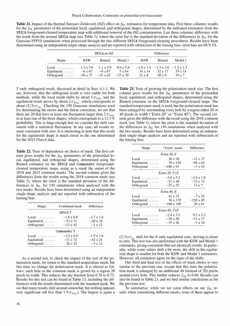
Planck Collaboration: Constraints on primordial non-Gaussianity
Table 21. Impact of the thermal Sunyaev-Zeldovich (tSZ) effect on fNL estimators for temperature data. First three columns: resultsfor the fNL parameters of the primordial local, equilateral, and orthogonal shapes, determined by the indicated estimators from theSMICA foreground-cleaned temperature map with additional removal of the tSZ contamination. Last three columns: difference withthe result from the normal SMICA map (see Table 5), where the error bar is the standard deviation of the differences in fNL for theGaussian FFP10 simulations when processed through the two different SMICA foreground-cleaning procedures. Results have beendetermined using an independent single-shape analysis and are reported with subtraction of the lensing bias; error bars are 68 % CL.
SMICA no-SZ Difference
Shape KSW Binned Modal 1 KSW Binned Modal 1
Local . . . . . . . . . 1.3 ± 5.6 1.1 ± 5.9 0.9 ± 5.8 −1.8 ± 1.4 −1.3 ± 1.6 −1.5 ± 1.3Equilateral . . . . . . −6 ± 67 −6 ± 67 5 ± 64 14 ± 14 32 ± 17 19 ± 14Orthogonal . . . . . −36 ± 37 −31 ± 42 −23 ± 39 21 ± 8 20 ± 9 19 ± 7
T-only orthogonal result, discussed in detail in Sect. 6.1.1. Wesee, however, that the orthogonal result is very stable for bothmethods, while the local result shifts by about 1σ∆ fNL and theequilateral result moves by about 2σ∆ fNL , which corresponds toabout (2/3)σ fNL . Checking the 150 Gaussian simulations usedfor determining the errors and the linear correction, we see thatthere are 20 that have at least one fluctuation larger than 2σ∆ fNL
in at least one of the three shapes, which corresponds to a 13.3 %probability. This is large enough that we consider the shift con-sistent with a statistical fluctuation. In any case, all results re-main consistent with zero. It is interesting to note that this resultfor the equilateral shape is much closer to the one determinedfor the 2015 Planck data.
Table 22. Tests of dependence on choice of mask. The first col-umn gives results for the fNL parameters of the primordial lo-cal, equilateral, and orthogonal shapes, determined using theBinned estimator on the SMICA and Commander foreground-cleaned temperature maps, using as a mask the union of the2018 and 2015 common masks. The second column gives thedifferences from the results using the 2018 common mask (seeTable 5), where the error is the standard deviation of the dif-ferences in fNL for 150 simulations when analysed with thetwo masks. Results have been determined using an independentsingle-shape analysis and are reported with subtraction of thelensing bias.
Shape Combined mask Difference
SMICA TLocal . . . . . . . . . −1.8 ± 6.0 −1.7 ± 1.6Equilateral . . . . . . −23 ± 71 −49 ± 24Orthogonal . . . . . −13 ± 42 −1 ± 12
Commander TLocal . . . . . . . . . −3.2 ± 6.0 −1.9 ± 1.6Equilateral . . . . . . −11 ± 72 −42 ± 24Orthogonal . . . . . 26 ± 43 −3 ± 12
As a second test, to check the impact of the size of the po-larization mask, we return to the standard temperature mask, butthis time we change the polarization mask. It is altered as fol-lows: each hole in the common mask is grown by a region 20pixels in width. This reduces the sky fraction from 0.78 to 0.73.Results for this test can be found in Table 23, including the dif-ferences with the results determined with the standard mask. Wesee that many results shift around somewhat, but nothing appearsvery significant (all less than 1.5σ∆ fNL ). The largest is again a
Table 23. Tests of growing the polarization mask size. The firstcolumn gives results for the fNL parameters of the primordiallocal, equilateral, and orthogonal shapes, determined using theBinned estimator on the SMICA foreground-cleaned maps. Thestandard temperature mask is used, but the polarization mask hasbeen enlarged by surrounding every hole by a region either 20 or40 pixels in width (“Extra 20” or “Extra 40”). The second col-umn gives the difference with the result using the 2018 commonmask (see Table 5), where the error is the standard deviation ofthe differences in fNL for 150 simulations when analysed withthe two masks. Results have been determined using an indepen-dent single-shape analysis and are reported with subtraction ofthe lensing bias.
Shape “Extra” mask Difference
Extra 20, ELocal . . . . . . . . . 36 ± 28 −12 ± 17Equilateral . . . . . . 70 ± 150 −96 ± 65Orthogonal . . . . . −180 ± 91 −3 ± 43
Extra 20, T+ELocal . . . . . . . . . −5.0 ± 5.2 −2.4 ± 1.8Equilateral . . . . . . −31 ± 48 −12 ± 13Orthogonal . . . . . −23 ± 25 11 ± 7
Extra 40, ELocal . . . . . . . . . 41 ± 33 −7 ± 22Equilateral . . . . . . 16 ± 170 −150 ± 85Orthogonal . . . . . −160 ± 100 20 ± 61
Extra 40, T+ELocal . . . . . . . . . −2.4 ± 5.2 0.2 ± 2.2Equilateral . . . . . . −30 ± 50 −11 ± 17Orthogonal . . . . . −35 ± 26 −1 ± 10
(2/3)σ fNL shift for the E-only equilateral case, moving it closerto zero. This test was also performed with the KSW and Modal 1estimators, giving consistent (but not identical) results. In partic-ular, while some values shift a bit more, the shift in the equilat-eral shape is smaller for both the KSW and Modal 1 estimators.However, all estimators agree on the signs of the shifts.
Our third and final test of the effects of mask choice is verysimilar to the previous one, except that this time the polariza-tion mask is enlarged by an additional 40 (instead of 20) pixelsaround every hole. This further reduces fsky to 0.66. Results canalso be found in Table 23, and we find similar conclusions as forthe previous test.
To summarize, while we see some effects on our fNL re-sults when considering different masks, none of these appear to
36

Planck Collaboration: Constraints on primordial non-Gaussianity
Fig. 17. Evolution of the fNL parameters (solid blue line with data points) and their uncertainties (dotted blue lines) for the threeprimordial bispectrum templates as a function of the minimum multipole number `min used in the analysis. From left to right thepanels show local, equilateral, and orthogonal shape results, while the different rows from top to bottom show results for T only, Eonly, and full T+E data. To indicate more clearly the evolution of the uncertainties, they are also plotted around the final value offNL (solid green lines without data points, around the horizontal dashed green line). The results here have been determined with theBinned bispectrum estimator for the SMICA map, assume all shapes to be independent, and the lensing bias has been subtracted.
be significant (further reinforced by the fact that the shifts varysomewhat between estimators), nor do they change the conclu-sions of our paper.
6.5. Dependence on multipole number
As in previous releases we also test the dependence of the resultsfor fNL on the choice of `min and `max used in the analysis. Thistest is most easily performed using the Binned estimator. Resultsare shown in Fig. 17 for the dependence on `min and in Fig. 18for the dependence on `max.
Considering first Fig. 17, for `min, the plots look very sim-ilar to the ones in the paper investigating the 2015 Planck data(PCNG15), with increased stability for the E-only local results.As explained in Sect. 3.2.2, it was decided to use `min = 4 forthe polarization maps, since there was an issue with bias andincreased variance when the two lowest multipoles for E wereincluded. However, this still allows us to use many more low-`polarization modes than for the 2015 data, when it was necessaryto adopt `min = 40 for polarization.
Turning to Fig. 18, for `max, we also notice good agreementwith the analysis of the 2015 data, and slightly more stable re-sults (e.g., for T -only equilateral). We see that the T-only resultshave stabilized by ` = 2000 and the E-only results by ` = 1500,so that there is no problem with the KSW and Modal estimatorsusing these lower values for `max. As before we also confirm the“WMAP excess” for the local shape at ` ≈ 500 (Bennett et al.2013), even more clearly than in PCNG15. However, this doesnot appear to be a major outlier when considering all values of`max and all possible shapes.
6.6. Summary of validation tests
Throughout this section we have discussed a set of tests aimedat evaluating the robustness of our results. For convenience, wesummarize here our main findings.
– We find good consistency for fNL local, equilateral, and or-thogonal measurements, between all component-separationmethods and with all bispectrum estimators, separately con-sidering T-only, E-only, and T+E results. The agreement for
37

Planck Collaboration: Constraints on primordial non-Gaussianity
Fig. 18. Same as Fig. 17, but this time as a function of the maximum multipole number `max used in the analysis.
E-only results has significantly improved with respect to theprevious release.
– The possible exception is provided by the orthogonal T-only estimates. In this case, a comparison with simula-tions shows significant differences in specific cases, namelySMICA – Commander and, to a lesser extent, SMICA – SEVEM.However, these differences are coming from fluctuations infNL for Commander and SEVEM with respect to the two previ-ous Planck releases, when all temperature maps were alwaysin excellent agreement. Our main SMICA results are, on theother hand, completely stable. Moreover, the discrepancy be-comes much less significant when adding polarization, it islimited to one specific shape, and it is in any case at a levelthat does not alter the interpretation of the results. Therefore,in the end, we do not consider this issue to be problematic.
– Nevertheless, in light of this test, we are led to a slight pref-erence for SMICA and NILC as methods of choice for primor-dial NG analysis. Given that SMICA also gave a slightly bet-ter performance for NG analysis in the two previous releases,and that results extracted from SMICA maps have been quitestable over time, we maintain SMICA as our final choice, asalready justified in detail in the papers analysing the 2013and 2015 Planck data (PCNG13; PCNG15).
– We find very good consistency between fully reconstructedbispectra, for different component-separation methods, us-ing both the Modal and the Binned approaches. Polarization-
only bispectra again show a large improvement compared tothe previous analysis of Planck data.
– The observed noise mismatch between the data and theFFP10 simulations does not seem to impact our results. Ourcubic statistics cannot be biased by this mismatch, and testson simulations show that the effect on fNL errors is negligi-ble.
– Results are stable to changes in sky coverage and differentcuts in the multipole domain. Restricting the analysis to themultipole range probed by WMAP shows good agreementbetween WMAP and Planck.
– We find no sign of any residual Galactic thermal dust con-tamination in the Planck component-separated CMB maps.
– Contamination from the thermal SZ effect on the standardprimordial and lensing T-only results is not at a significantlevel, compared to statistical errors.
Overall, the results display a high level of internal consistency,and are notably characterized by a large improvement in thequality of polarization-only bispectra with respect to the previ-ous release. Whereas in 2015 we cautioned the reader to takepolarization-based fNL estimates as preliminary, we can nowstate that our T+E-based constraints are fully robust. This is oneof the main conclusions of this paper.
38

Planck Collaboration: Constraints on primordial non-Gaussianity
7. Limits on the primordial trispectrum
We will now present constraints on three shapes for the primor-dial four-point function or trispectrum, denoted glocal
NL , gσ4
NL, and
g(∂σ)4
NL , and described below.The details of the analysis are mostly unchanged from the pa-
per analysing the 2015 Planck data (see section 9 of PCNG15).Nevertheless, we briefly review the four-point analysis here; formore details, see PCNG15, or Smith et al. (2015), which con-tains technical details of the pipeline.
First, we describe the three different signals of interest. Thelocal-type trispectrum glocal
NL arises if the initial adiabatic curva-ture ζ is given by the following non-Gaussian model:
ζ(x) = ζG(x) +9
25glocal
NL ζG(x)3 (42)
where ζG is a Gaussian field. The trispectrum in the local modelis given by
〈ζk1ζk2ζk3ζk4〉′ =
5425
glocalNL
[Pζ(k1)Pζ(k2)Pζ(k3) + 3 perms.
].
(43)In this equation and throughout this section, a “primed” four-point function denotes the four-point function without itsmomentum-conserving delta function, i.e.,
〈ζk1ζk2ζk3ζk4〉 = 〈ζk1ζk2ζk3ζk4〉′(2π)3δ(3)
(∑ki
)+ disc., (44)
where “+ disc.” denotes disconnected contributions to the 4-point function. It can be shown that the local-type trispectrumin Eq. (43) is always negligibly small in single-field inflation(Senatore & Zaldarriaga 2012a); however, it can be large in mul-tifield models of inflation in which a large bispectrum is forbid-den by symmetry (Senatore & Zaldarriaga 2012b).
The next two shapes gσ4
NL, g(∂σ)4
NL are generated by the opera-tors σ4 and (∂iσ)2(∂ jσ)2 in the effective field theory (EFT) ofinflation (Bartolo et al. 2010b; Senatore & Zaldarriaga 2012b;Smith et al. 2015). For data analysis purposes, they can be de-fined by the following trispectra:
〈ζk1ζk2ζk3ζk4〉′ =
921625
gσ4
NLA3ζ
∫ 0
−∞
dτE τ4E
4∏i=1
ekiτE
ki
=
22118425
gσ4
NL A3ζ
1k1k2k3k4K5 ; (45)
〈ζk1ζk2ζk3ζk4〉′ =
829442575
g(∂σ)4
NL A3ζ
∫ 0
−∞
dτE
4∏i=1
(1 − kiτE)ekiτE
k3i
×
[(k1 · k2)(k3 · k4) + 2 perms.
]=
1658882575
g(∂σ)4
NL A3ζ
×
2K4 − 2K2 ∑k2
i + K∑
k3i + 12k1k2k3k4
k31k3
2k33k3
4K5
×
[(k1 · k2)(k3 · k4) + 2 perms.
]. (46)
Here K =∑
i ki, and numerical prefactors have been chosen sothat the trispectra have the same normalization as the local shapein Eq. (43) when restricted to tetrahedral wavenumber configura-tions with |ki| = k and (ki · k j) = −k2/3. We mention in advancethat there is another shape gσ
2(∂σ)2
NL that arises at the same orderin the EFT expansion, to be discussed at the end of this section.
In Eqs. (45) and (46), we have written each trispectrum intwo algebraically equivalent ways, an integral representation andan “integrated” form. The integral representation arises naturallywhen evaluating the Feynman diagram for the EFT operator. Italso turns out to be useful for data analysis, since the resulting“factorizable” representation for the trispectrum leads to an ef-ficient algorithm for evaluating the CMB trispectrum estimator(Planck Collaboration XVII 2016; Smith et al. 2015).
For simplicity in Eqs. (45) and (46), we have assumed ascale-invariant power spectrum Pζ(k) = Aζ/k3. For the Planckanalysis, we slightly modify these trispectra to a power-law spec-trum Pζ(k) ∝ kns−4, as described in appendix C of Smith et al.(2015).
To estimate each gNL parameter from Planck data, we use the“pure-MC” trispectrum estimation pipeline from section IX.B ofSmith et al. (2015). In this pipeline, the data are specified as afiltered harmonic space map d`m, and its covariance is character-ized via a set of 1000 filtered signal + noise simulations.
The “filter” is an experiment-specific linear operation whoseinput consists of one or more pixel-space maps, and whose out-put is a single harmonic-space map, d`m. In the Planck trispec-trum analysis, we define the filter as follows. First, we take thesingle-frequency pixel-space maps, and combine them to ob-tain a single component-separated pixel-space map, using oneof the component-separation algorithms, SMICA, SEVEM, NILC,Commander, or SMICA no-SZ (a variant of the SMICA algorithmthat guarantees zero response to Compton-y sources, at the ex-pense of slightly higher noise; see Sect. 6.3.2). Second, we sub-tract the best-fit monopole and dipole, inpaint masked pointsources, and apodize the Galactic plane boundary. The details ofthese steps are unchanged from the 2015 Planck data analysis,and are described in section 9.1 of PCNG15. Third, we take thespherical transform of the pixel-space map out to lmax = 1600,obtaining a harmonic-space map d`m. Finally, we define the fil-tered map d`m by applying the multiplicative factor:
d`m =d`m
b`C` + b−1`
N`
. (47)
This sequence of steps defines a linear operation, whose inputis a set of single-frequency pixel-space maps, and whose outputis a filtered harmonic-space map d`m. This filtering operation isused as a building block in the trispectrum pipeline described inSmith et al. (2015), and is the only part of the pipeline that isPlanck-specific.
The results of the analysis, for all three trispectrum shapesand five different component-separation algorithms, are pre-sented in Table 24. We do not find evidence for a nonzero pri-mordial trispectrum.
Each entry in Table 24 is a constraint on a single gNL-parameter with the others held fixed. We next consider joint con-straints involving multiple gNL-parameters. In this case, we needto know the covariance matrix between gNL-parameters. We findthat
Corr(gσ4
NL, g(∂σ)4
NL ) = 0.61, (48)
and the correlation between glocalNL and the other two gNL-
parameters is negligible.Multifield models of inflation will generally predict a linear
combination of the quartic operators σ4 and (∂iσ)2(∂ jσ)2. In ad-dition, there is a third operator σ2(∂iσ)2 that arises at the sameorder in the EFT expansion. For completeness, its trispectrum is
39

Planck Collaboration: Constraints on primordial non-Gaussianity
Table 24. Planck 2018 constraints on the trispectrum parameters glocalNL , gσ
4
NL, and g(∂σ)4
NL from different component-separated maps.
glocalNL gσ
4
NL g(∂σ)4
NL
SMICA . . . . . . . . . . . . . (−5.8 ± 6.5) × 104 (−0.8 ± 1.9) × 106 (−3.9 ± 3.9) × 105
SMICA no-SZ . . . . . . . . (−12.3 ± 6.6) × 104 (−0.6 ± 1.9) × 106 (−3.5 ± 3.9) × 105
SEVEM . . . . . . . . . . . . . (−5.5 ± 6.5) × 104 (−0.8 ± 1.9) × 106 (−3.2 ± 3.9) × 105
NILC . . . . . . . . . . . . . . (−3.6 ± 6.3) × 104 (−0.8 ± 1.9) × 106 (−4.0 ± 3.9) × 105
Commander . . . . . . . . . (−8.1 ± 6.5) × 104 (−0.8 ± 1.9) × 106 (−3.5 ± 3.9) × 105
given by
〈ζk1ζk2ζk3ζk4〉′ = −
13824325
gσ2(∂σ)2
NL A3ζ
∫ 0
−∞
dτE τ2E
×
[(1 − k3τE)(1 − k4τE)
k1k2k33k3
4(k3 · k4) e
∑kiτE + 5 perms.
]= −
27648325
gσ2(∂σ)2
NL A3ζ
×
[K2 + 3(k3 + k4)K + 12k3k4
k1k2k33k3
4K5 (k3 · k4)+5 perms.].
(49)
However, a Fisher matrix analysis shows that this trispectrum isnearly 100 % correlated with the σ4 and (∂iσ)2(∂ jσ)2 trispectra.If the parameter gσ
2(∂σ)2
NL is non-zero, then we can absorb it into
the “effective” values of the parameters gσ4
NL and g(∂σ)4
NL as
(gσ4
NL)eff = 0.59 gσ2(∂σ)2
NL ,
(g(∂σ)4
NL )eff = 0.091 gσ2(∂σ)2
NL . (50)
Therefore, to study joint constraints involving multiple gNL pa-rameters, it suffices to consider the two parameters, gσ
4
NL and
g(∂σ)4
NL , with correlation coefficient given in Eq. (48).We define the two-component parameter vector
gi =
gσ4
NL
g(∂σ)4
NL
. (51)
and let gi denote the two-component vector of single-gNL esti-mates from the SMICA maps (Table 24):
gi =
(−8.0−3.9
)× 10−5. (52)
We also define a two-by-two Fisher matrix Fi j, whose diagonalis given by Fii = 1/σ2
i , whereσi is the single-gNL statistical errorin Table 24, and whose off-diagonal is F12 = rF1/2
11 F1/222 , where r
is the correlation in Eq. (48). This gives:
Fi j =
(2.8 8.38.3 66.5
)× 10−13. (53)
Now, given a set of “theory” gNL values, represented by a two-vector gi, we compare to the Planck data by computing the fol-lowing quantity for the trispectrum:
χ2(gi) =[Fiigi − (Fg)i
]F−1
i j[F j jg j − (Fg) j
]. (54)
In a model-building context where the gNL quantities gi de-pend on model parameters, confidence regions on model param-eters can be obtained by appropriately thresholding χ2. We givesome examples in Sect. 8.
8. Implications for early-Universe physics
We now want to convert constraints on primordial NG into con-straints on parameters of various models of inflation. This allowsus to highlight the constraining power of NG measurements,as an additional complementary observable beyond the CMBpower spectra. In particular NG constraints can severely limitthe parameter space of models that are alternatives to the stan-dard single-field models of slow-roll inflation, since they typi-cally feature a higher level of NG.
Unless stated otherwise, we follow the same proceduresadopted in PCNG13 and PCNG15. A posterior of the model pa-rameters is built based on the following steps: we start from theassumption that the sampling distribution is Gaussian (which issupported by Gaussian simulations); the likelihood is approxi-mated by the sampling distribution, but centred on the NG esti-mate (see Elsner & Wandelt 2009); we use uniform or Jeffreys’priors, over intervals of the model parameter space that are phys-ically meaningful (or as otherwise stated); and in some caseswhere two or more parameters are involved, we marginalize theposterior to provide one-dimensional limits on the parameter un-der consideration.
8.1. General single-field models of inflation
DBI models Dirac-Born-Infeld (DBI) models of inflation(Silverstein & Tong 2004; Alishahiha et al. 2004) arise fromhigh-energy string-theory constructions and generate a nonlin-earity parameter f DBI
NL = −(35/108)(c−2s − 1), where cs is the
sound speed of the inflaton perturbations (Silverstein & Tong2004; Alishahiha et al. 2004; Chen et al. 2007b). The enhance-ment of the NG amplitude due to a possible sound speed cs < 1arises from a non-standard kinetic term of the inflaton field.Notice that we have constrained the exact theoretical (non-separable) shape (see equation 7 of PCNG13), even though it isvery similar to the equilateral type. Our constraint f DBI
NL = 46±58from temperature data ( f DBI
NL = 14 ± 38 from temperature andpolarization) at 68 % CL (with lensing and point sources sub-tracted, see Table 11) implies
cDBIs ≥ 0.079 (95 %, T only) , (55)
andcDBI
s ≥ 0.086 (95 %, T+E) . (56)
Implications for the effective field theory of inflation Now wecan update CMB limits on the speed of sound cs at which inflatonfluctuations propagated in the very early Universe. A very gen-eral constraint on this inflationary parameter can be obtained byemploying the EFT approach to inflation (Cheung et al. 2008;Weinberg 2008, and see Sect. 7). This approach allows us toobtain predictions for the parameter space of primordial NGthrough a general characterization of the inflaton field inter-actions. The Lagrangian of the system is expanded into the
40

Planck Collaboration: Constraints on primordial non-Gaussianity
dominant operators that respect some underlying symmetries.The procedure thus determines a unifying scheme for classesof models featuring deviations from single-field slow-roll infla-tion. Typically the equilateral and orthogonal templates repre-sent an accurate basis to describe the full parameter space ofEFT single-field models of inflation, and therefore we will usethe constraints on f equil
NL and f orthoNL .
As a concrete example, let us consider the Lagrangian ofgeneral single-field models of inflation (of the form P(X, ϕ) mod-els, where X = gµν∂µφ ∂νφ) written with the EFT approach:
S =
∫d4x√−g
− M2PlH
c2s
(π2 − c2
s(∂iπ)2
a2
)−M2
PlH(1 − c−2s )π
(∂iπ)2
a2 +
(M2
PlH(1 − c−2s ) −
43
M43
)π3
].
(57)
The scalar perturbation π generates the curvature perturbationζ = −Hπ. In this case there are two relevant inflaton interactions,π(∂iπ)2 and (π)3, producing two specific bispectra with ampli-tudes f EFT1
NL = −(85/324)(c−2s − 1) and f EFT2
NL = −(10/243)(c−2s −
1)[c3 + (3/2)c2
s
], respectively. Here M3 is the amplitude of
the operator π3 (see Senatore et al. 2010; Chen et al. 2007b;Chen 2010b), with the dimensionless parameter c3(c−2
s − 1) =2M4
3c2s/(HM2
Pl) (Senatore et al. 2010). The two EFT shapes canbe projected onto the equilateral and orthogonal shapes, with themean values of the estimators for f equil
NL and f orthoNL expressed in
terms of cs and c3 as
f equilNL =
1 − c2s
c2s
[−0.275 − 0.0780c2
s − (2/3) × 0.780c3
],
f orthoNL =
1 − c2s
c2s
[0.0159 − 0.0167c2
s − (2/3) × 0.0167c3
], (58)
where the coefficients come from the Fisher matrix between thetheoretical bispectra predicted by the two operators π(∇π)2 andπ3 and the equilateral and orthogonal templates. Notice that DBImodels reduce to the condition c3 = 3(1 − c2
s )/2, while the non-interacting (vanishing NG) case corresponds to cs = 1 and M3 =0 (or c3(c−2
s − 1) = 0).We then proceed as in the two previous analyses
(PCNG13; PCNG15). We employ a χ2 statistic computed asχ2(c3, cs) = uT(c3, cs)C−1u(c3, cs), with vi(c3, cs) = f i(c3, cs) − f i
P(i=equilateral, orthogonal), where f i
P are the joint estimatesof equilateral and orthogonal fNL values (see Table 6), whilef i(c3, cs) are provided by Eq. (58) and C is the covariance ma-trix of the joint estimators. Figure 19 shows the 68 %, 95 %, and99.7 % confidence regions for f equil
NL and f orthoNL , as derived from
from the T +E constraints, with the requirement χ2 ≤ 2.28, 5.99,and 11.62, respectively (corresponding to a χ2 variable with twodegrees of freedom). In Fig. 20 we show the corresponding con-fidence regions in the (c3, cs) parameter space. Marginalizingover c3 we find
cs ≥ 0.021 (95 %, T only) , (59)and
cs ≥ 0.021 (95 %, T+E) . (60)
There is a slight improvement in comparison with the constraintsobtained in PCNG15 coming from the T + E data.
-400 -200 0 200 400-20
0-
100
010
020
0
fNLequil
fN
Lorth
o
Fig. 19. 68 %, 95 %, and 99.7 % confidence regions in the param-eter space ( f equil
NL , f orthoNL ), defined by thresholding χ2, as described
in the text.
0.01 0.02 0.05 0.1 0.2 0.5 1
-15
000-
1000
0-
5000
050
00
0.01 0.02 0.05 0.1 0.2 0.5 1
cs
c3
Ics-
2-
1M
Fig. 20. 68 %, 95 %, and 99.7 % confidence regions in the single-field inflation parameter space (cs, c3), obtained from Fig. 19 viathe change of variables in Eq. (58).
8.2. Multi-field models
Constraints on primordial NG of the local type lead to strongimplications for models of inflation where scalar fields (differentfrom the inflaton) are dynamically important for the generationof the primordial curvature perturbation. In the following we testtwo scenarios for curvaton models.
Basic curvaton models The simplest adiabatic curvaton mod-els predict primordial NG of the local shape with a nonlinearity
41
Planck Collaboration: Constraints on primordial non-Gaussianity
parameter (Bartolo et al. 2004d,c)
f localNL =
54rD−
5rD
6−
53, (61)
in the case where the curvaton field has a quadratic poten-tial (Lyth & Wands 2002; Lyth et al. 2003; Lyth & Rodriguez2005; Malik & Lyth 2006; Sasaki et al. 2006). Here the param-eter rD = [3ρcurvaton/(3ρcurvaton + 4ρradiation)]D is the “curvatondecay fraction” at the time of the curvaton decay in the suddendecay approximation. We assume a uniform prior, 0 < rD < 1.It is worth recalling that these models predict a lower bound forthe level of NG, of the order of unity (corresponding preciselyto f local
NL = −5/4), which is considered as a typical threshold todistinguish between standard single-field and multi-field scenar-ios. Our constraint f local
NL = −0.5 ± 5.6 at 68 % CL (see Table 6)implies
rD ≥ 0.19 (95 %, T only) . (62)
The constraint f localNL = −0.9 ± 5.1 at 68 % CL obtained from
temperature and polarization data yields the constraint
rD ≥ 0.21 (95 %, T +E) . (63)
These limits indicate that in such scenarios the curvaton fieldhas a non-negligible energy density when it decays. Meaningfulimprovements are achieved with respect to previous bounds inPCNG15, namely an almost 20 % improvement from T -onlydata and a 10 % improvement when including E-mode polariza-tion.
Decay into curvaton particles We reach similar improvementson the parameters of the second scenario of the curvaton mod-els we consider. In this case one accounts for the possibil-ity that the inflaton field can decay into curvaton particles(Linde & Mukhanov 2006), a possibility that is neglected in theabove expression (Eq. 61) for f local
NL . It might be the case that theclassical curvaton field survives and begins to dominate. In thiscase also the curvaton particles produced during reheating areexpected to survive and dominate over other species at the epochof their decay (since thay have the same equation of state asthe classical curvaton field). Primordial adiabatic perturbationsare generated given that the classical curvaton field and the cur-vaton particles decay at the same time (see Linde & Mukhanov2006 for a detailed discussion). To interpret fNL in this scenariowe employ the general formula for f local
NL derived in Sasaki et al.(2006), which takes into account the possibility that the inflatonfield decays into curvaton particles:
f localNL = (1 + ∆2
s )5
4rD−
5rD
6−
53. (64)
Here the parameter ∆2s is the ratio of the energy density of curva-
ton particles to the energy density of the classical curvaton field(Linde & Mukhanov 2006; Sasaki et al. 2006), while now ρcurvin the expression for rD must be replaced by the sum of the den-sities of the curvaton particles and curvaton field. As in PCNG15we use uniform priors 0 < rD < 1 and 0 < ∆2
s < 102. Our limitson f local
NL constrain
∆2s ≤ 6.9 (95 %, T only) , (65)
and∆2
s ≤ 6.2 (95 %, T +E) , (66)
which does not exclude a contribution of curvaton particles com-parable to the one from the classical curvaton field.
8.3. Non-standard inflation models
Directional-dependent NG Table 13 shows the constraints ondirectionally-dependent bispectra (Eq. 20). This kind of NG ispredicted by several different inflationary models. For example,it is a robust and (almost unavoidable) outcome of models ofinflation where scale-invariant gauge fields are present duringinflation. As summarized in Sect. 2 they are also produced frompartially massless higher-spin particles (Franciolini et al. 2018)or from models of solid inflation (Endlich et al. 2013, 2014;Shiraishi et al. 2013a), as well as in models of inflation thatbreak both rotational and parity invariance (Bartolo et al. 2015).To compare with the constraints obtained in the analysis of the2015 Planck data (PCNG15), we reconsider the specific modelwhere the inflaton is coupled to the kinetic term F2 of a gaugefield via a term L= − I2(φ)F2/4, where I(φ) is a function thatdepends on the inflaton field, having an appropriate time evolu-tion during inflation (see, e.g., Ratra 1992). Specifically in thesemodels the production of super-horizon vector field perturba-tions switches on the L = 0 and L = 2 modes in the bispectrum,with nonlinearity parameters f L
NL = XL(|g∗|/0.1) (Nk3/60), withXL=0 = (80/3) and XL=2 = −(10/6), respectively (Barnaby et al.2012; Bartolo et al. 2013a; Shiraishi et al. 2013a). In these ex-pressions g∗ is a parameter that measures the amplitude ofa quadrupolar anisotropy in the power spectrum (see, e.g.,Ackerman et al. 2007), while N is the number of e-folds (fromthe the end of inflation) at which the relevant scales cross outsidethe Hubble scale. It is therefore interesting to set some limits onthe parameter g∗ exploiting the constraints from primordial NGof this type. Using the SMICA constraints from T (or T+E) inTable 13, marginalizing over a uniform prior 50 ≤ N ≤ 70,and assuming uniform priors on −1 ≤ g∗ ≤ 1, we obtain the95 % bounds −0.041 < g∗ < 0.041 (−0.036 < g∗ < 0.036), and−0.35 < g∗ < 0.35 (−0.30 < g∗ < 0.30), from the L = 0 andL = 2 modes, respectively (considering g∗ to be scale indepen-dent).
Tensor NG and pseudoscalars Using the SMICA T+E resultf tensNL = (8 ± 11) × 102 (68 % CL), we here place constraints
on two specific inflation models, including either a U(1)-axioncoupling or an SU(2)-axion one. The former U(1) model resultsin f tens
NL ≈ 6.4 × 10¹¹P3ε3e6πξ/ξ9, where P is the vacuum-modecurvature power spectrum, ε is a slow-roll parameter of the in-flaton field, and ξ expresses the strength of the U(1)-axion cou-pling (Cook & Sorbo 2013; Shiraishi et al. 2013b). We then fixε to be 0.01 and marginalize P with the prior, 1.5 × 10⁻⁹ < P <3.0×10⁻⁹; assuming a prior, 0.1 < ξ < 7.0, the upper bound on ξis derived as ξ < 3.3 (95 % CL). In the latter SU(2) model, underone specific condition, the tensor nonlinear parameter is relatedto the tensor-to-scalar ratio r and the energy density fraction ofthe gauge field ΩA as f tens
NL ≈ 2.5r2/ΩA (Agrawal et al. 2018).The lower bound on ΩA is estimated under a prior, 0 < ΩA < 1.We find ΩA > 2.3 × 10⁻⁷ and 2.7 × 10⁻⁹ (95 % CL) for r = 10−2
and 10−3, respectively.
Warm inflation As in previous analyses (PCNG13; PCNG15),we adopt the expression f warm
NL = −15 ln (1 + rd/14) − 5/2(Moss & Xiong 2007). This is valid when dissipative effects arestrong, i.e., for values rd & 2.5 of the dissipation parameterrd = Γ/(3H) (measuring the effectiveness of the energy trans-fer from the inflaton field to radiation).13 Assuming a constant
13 The intermediate and weak dissipative regimes (rd ≤ 1) predict anNG amplitude with a strong dependence on the microscopic parameters
42
Planck Collaboration: Constraints on primordial non-Gaussianity
prior 0 ≤ log10 rd ≤ 4, the SMICA constraints f warmSNL = −39 ± 44
(at 68 % CL) from T and f warmSNL = −48 ± 27 from T+E (see
Table 12), yield log10 rd ≤ 3.6 and log10 rd ≤ 3.5, respectively,at 95 % CL. The results show that strong-dissipative effects inwarm inflation models remain allowed. This is a regime wheregravitino overproduction problems can be evaded (for a discus-sion see Hall & Peiris 2008).
8.4. Alternatives to inflation
As an example we update the constraints on some ekpy-rotic/cyclic models (e.g., see Lehners 2010 for a review).Typically local NG is produced through a conversion of “intrin-sic” non-Gaussianity in the entropy fluctuations into the curva-ture perturbation. This conversion can proceed in different ways.The “ekpyrotic conversion” models, for which the conversionacts during the ekpyrotic phase, have already been ruled out(Koyama et al. 2007, PCNG13). On the other hand, in the “ki-netic conversion” models the conversion takes place after theekpyrotic phase and a local bispectrum is generated with anamplitude f local
NL = (3/2) κ3√ε ± 5.14 The sign depends on the
details of the conversion process (Lehners & Steinhardt 2008;Lehners 2010; Lehners & Steinhardt 2013), and typical valuesof the parameter ε are ε ≈ 50 or greater. Assuming ε ≈ 100and using a uniform prior on −5 < κ3 < 5 the constraints onf localNL from T only (see Table 6), implies −1.1 < κ3 < 0.36 and−0.43 < κ3 < 1.0 at 95 % CL, for the plus and minus sign inf localNL , respectively. The T+E constraints on f local
NL (Table 6) yield−1.05 < κ3 < 0.27 and −0.38 < κ3 < 0.94 at 95 % CL, forthe plus and minus sign, respectively. If we take ε ≈ 50 as anexample, we obtain the following limits: −1.6 < κ3 < 0.51 and−0.62 < κ3 < 1.5 at 95 % CL from T only; and −1.5 < κ3 < 0.39and −0.54 < κ3 < 1.3 at 95 % CL from T+E constraints.
8.5. Inflationary interpretation of CMB trispectrum results
We briefly analyze inflationary implications of the Plancktrispectrum constraints, using the SMICA limits on gNL param-eters from Table 24.
First, we consider single-field inflationary models, using theeffective action for the Goldstone boson π (see, e.g., Smith et al.2015):
S π =
∫d4x√−g
− M2
PlH(∂µπ
)2
+ 2M42
[π2 + π3 − π
(∂iπ)2
a2 + (∂µπ)2(∂νπ)2]
−M4
3
3!
[8 π3 + 12π2(∂µπ)2 + · · ·
]+
M44
4!
[16 π4 + 32π3(∂µπ)2 + · · ·
]+ · · ·
, (67)
The mass scale M4 is related to our previously-defined gNL pa-rameters by:
gσ4
NL =25
288M4
4
H4 Aζ c3s . (68)
(T/H and rd), giving rise to a different additional bispectrum shape (seeBastero-Gil et al. 2014).
14 There might also be the case where the intrinsic NG is vanishingand primordial NG is generated only by nonlinearities in the conversionprocess, reaching an amplitude f local
NL ≈ ±5 (Qiu et al. 2013; Li 2013;Fertig et al. 2014).
Therefore, using the gσ4
NL limit from Table 24, we get the follow-ing constraint on single-field models:
− 12.8 × 10¹⁴ <M4
4
H4c3s< 8.2 × 10¹⁴ (95 % CL). (69)
Next consider the case of multifield inflation. Here, we consideran action of the more general form:
S σ =
∫d4x√−g
[12
(∂µσ)2 +1
Λ41
σ4
+1
Λ42
σ2(∂iσ)2 +1
Λ43
(∂iσ)2(∂ jσ)2], (70)
where σ is a light field that acquires quantum fluctuations withpower spectrum Pσ(k) = H2/(2k3). We assume that σ convertsto adiabatic curvature ζ, i.e. ζ = (2Aζ)1/2H−1σ. The model pa-rameters Λi are related to our previously-defined gNL parametersby:
gσ4
NLAζ =25
768H4
Λ41
,
gσ2(∂σ)2
NL Aζ = −325
6912H4
Λ42
, (71)
g(∂σ)4
NL Aζ =2575
20736H4
Λ43
,
and can be constrained by thresholding the χ2-statistic definedin Eq. (54). For example, to constrain the parameter Λ in theLorentz invariant model
S =
∫d4x√−g
[12
(∂µσ)2 +1
Λ4 (∂µσ)2(∂νσ)2], (72)
we set Λ41 = −2Λ4
2 = Λ43 = Λ4, obtain gNL-values using Eq. (71),
and use Eq. (54) to obtain χ2 as a function of Λ. We then thresh-old at ∆χ2 = 4 (as appropriate for one degree of freedom), toobtain the following constraint:
− 0.33 <H4
Λ4 < 0.11 (95 %). (73)
DBI Trispectrum We use the trispectrum constraints on theshape σ4 in Table 24 to determine a lower bound on the soundspeed of the inflaton field in DBI models. In fact in these mod-els the dominant contribution in the small-sound-speed limit(Chen et al. 2009; Arroja et al. 2009) to the contact interactiontrispectrum (Huang & Shiu 2006) produces such a shape, withan amplitude gσ
4
NL = −25/(768 c4s ). We employ the same proce-
dure described at the beginning of this section and, assuming auniform prior in the range 0 ≤ cs ≤ 1/5, we derive the followingconstraint on cs:
cDBIs ≥ 0.015 (95 %) . (74)
This constraint is independent from and consistent with thebounds of Eqs. (55) and (56) obtained from the bispectrum mea-surements. Notice that in the trispectrum case we are ignoringthe scalar exchange contribution, which turns out to be of thesame order in cs.
43

Planck Collaboration: Constraints on primordial non-Gaussianity
Curvaton trispectrum A generic prediction of the simplest adi-abatic curvaton scenario is also a local-type trispectrum with anamplitude glocal
NL given by (Sasaki et al. 2006)
glocalNL =
2554
(−
9rD
+12
+ 10rD + 3r2D
). (75)
Following the procedure described at the beginning of this sec-tion, we use the observational constraint obtained in Sect. 7 (seeTable 24), and the same uniform prior (0 < rD < 1) as inSect. 8.2, to obtain a lower bound on the curvaton decay frac-tion
rD ≥ 0.05 (95 %) . (76)
This limit is consistent with the previous ones derived using thebispectrum measurements and it is about a factor of 4 weaker.
9. Conclusions
In this paper, we have presented constraints on primordial NG,using the Planck full-mission CMB temperature and E-mode po-larization maps. Compared to the Planck 2015 release we nowinclude the low-` (4 ≤ ` < 40) polarization multipole range.
Our analysis produces the following final results (68 % CL,statistical): f local
NL = −0.9 ± 5.1; f equilNL = −26 ± 47; and f ortho
NL =−38 ± 24. These results are overall stable with respect to ourconstraints from the 2015 Planck data. They show no real im-provement in errors, despite the additional polarization modes.This is due to a combination of two factors. Firstly, the localshape, which is most sensitive to low-` modes and where onewould naively expect an improvement, is actually less sensitiveto polarization than the equilateral and orthogonal shapes. Thismeans that in the end none of the three shapes are very sensi-tive to low-` polarization modes. Secondly, the polarization sim-ulations used to determine the errors have a more realistic butslightly higher noise level than in the previous release.
On the other hand, the quality of polarization data shows aclear improvement with respect to our previous analysis. Thisis confirmed by a large battery of tests on our data set, in-cluding comparisons between different estimator implementa-tions (KSW, Binned, and two Modal estimators) and foreground-cleaning methods (SMICA, SEVEM, NILC, and Commander), stud-ies of robustness under changes in sky coverage and multipolerange, and an analysis of the impact of noise-related systemat-ics. While in our previous release we cautioned the reader to takepolarization bispectra and related constraints as preliminary, inlight of these tests we now consider our results based on the com-bined temperature and polarization data set to be fully reliable.This also implies that polarization-only, EEE bispectra can nowbe used for independent tests, leading to primordial NG con-straints at a sensitivity level comparable to that of WMAP fromtemperature bispectra, and yielding statistical agreement.
As in the previous analyses, we go beyond the local, equilat-eral, and orthogonal fNL constraints by considering a large num-ber of additional cases, such as scale-dependent feature and res-onance bispectra, running fNL models, isocurvature primordialNG, and parity-breaking models. We set tight constraints on allthese scenarios, but do not detect any significant signals.
On the other hand, the non-primordial lensing bispectrumis now detected with an improved significance compared to2015, excluding the null hypothesis at 3.5σ. The amplitude ofthe signal is consistent with the expectation from the Planckbest-fit cosmological parameters, further indicating the absenceof significant foreground contamination or spurious systematic
effects. We also explicitly checked for the presence of vari-ous non-primordial contaminants, like unclustered extragalacticpoint sources, CIB, Galactic thermal dust, and the thermal SZeffect, but apart from the first, none of these were detected. Thesmall amount of remaining point-source signal in the cleanedmaps has no impact on our other constraints because of its neg-ligible correlations.
We update our trispectrum constraints, now finding glocalNL =
(−5.8± 6.5)× 104 (68 % CL, statistical), while also constrainingadditional shapes, generated by different operators in an effectivefield-theory approach to inflation.
In addition to estimates of bispectrum and trispectrum ampli-tudes, we produce model-independent reconstructions and anal-yses of the Planck CMB bispectrum. Finally, we use our mea-surements to obtain constraints on early-Universe scenarios thatcan generate primordial NG. We consider, for example, generalsingle-field models of inflation, curvaton models, models withaxion fields producing parity-violating tensor bispectra, and in-flationary scenarios generating directionally-dependent bispec-tra (such as those involving vector fields).
In our data analysis efforts, which started with the 2013 re-lease, we achieved a number of crucial scientific goals. In par-ticular we reached an unprecedented level of sensitivity in thedetermination of the bispectrum and trispectrum amplitude pa-rameters ( fNL, gNL) and significantly extended the standard lo-cal, equilateral, and orthogonal analysis, encompassing a largenumber of additional shapes motivated by a variety of inflation-ary models. Moreover, we produced the first polarization-basedCMB bispectrum constraints and the first detection of the (non-primordial) bispectrum induced by correlations between CMBlensing and secondary anisotropies. Our stringent tests of manytypes of non-Gaussianity are fully consistent with expectationsfrom the standard single-field slow-roll paradigm and providestrong constraints on alternative scenarios. Nevertheless, the cur-rent level of sensitivity does not allow us to rule out or confirmmost alternative scenarios. It is natural at this stage to ask our-selves what should be the fNL sensitivity goal for future cosmo-logical experiments. A number of studies has identified fNL ∼ 1as a target. Achieving such sensitivity for local-type NG wouldenable us to either confirm or rule out a large class of multi-fieldmodels. A similar target for equilateral, orthogonal, and scale-dependent shapes would allow us to distinguish standard slow-roll from more complex single-field scenarios, such as thosecharacterized by higher-derivative kinetic terms or slow-roll-breaking features in the inflaton potential (see e.g., Alvarez et al.2014; Finelli et al. 2018, and references therein). With this aimin mind, the challenge for future cosmological observations willbe therefore that of reducing the fNL errors from this paper by atleast one order of magnitude.
Acknowledgements. The Planck Collaboration acknowledges the support of:ESA; CNES and CNRS/INSU-IN2P3-INP (France); ASI, CNR, and INAF(Italy); NASA and DoE (USA); STFC and UKSA (UK); CSIC, MINECO,JA, and RES (Spain); Tekes, AoF, and CSC (Finland); DLR and MPG(Germany); CSA (Canada); DTU Space (Denmark); SER/SSO (Switzerland);RCN (Norway); SFI (Ireland); FCT/MCTES (Portugal); and ERC and PRACE(EU). A description of the Planck Collaboration and a list of its members,indicating which technical or scientific activities they have been involved in,can be found at http://www.cosmos.esa.int/web/planck. Some of the re-sults in this paper have been derived using the HEALPix package. We also ac-knowledge the use of CAMB. Part of this work was undertaken on the STFCCOSMOS@DiRAC HPC Facility at the University of Cambridge, funded byUK BIS NEI grants. We gratefully acknowledge the IN2P3 Computer Center(http://cc.in2p3.fr) for providing a significant amount of the computingresources and services needed for the analysis. This research used resources ofthe National Energy Research Scientific Computing Center, a DOE Office ofScience User Facility supported by the Office of Science of the U.S. Department
44

Planck Collaboration: Constraints on primordial non-Gaussianity
of Energy under Contract No. DE-AC02-05CH11231. Some computations wereperformed on the GPC and Niagara cluster at the SciNet HPC Consortium;SciNet is funded by the Canada Foundation for Innovation under the auspicesof Compute Canada, the Government of Ontario, and the University of Toronto.
ReferencesAchucarro, A., Gong, J.-O., Hardeman, S., Palma, G. A., & Patil, S. P., Features
of heavy physics in the CMB power spectrum. 2011, J. Cosmology Astropart.Phys., 1, 30
Ackerman, L., Carroll, S. M., & Wise, M. B., Imprints of a primordial preferreddirection on the microwave background. 2007, Phys. Rev. D, 75, 083502
Adshead, P., Dvorkin, C., Hu, W., & Lim, E. A., Non-Gaussianity from stepfeatures in the inflationary potential. 2012, Phys. Rev. D, 85, 023531
Agrawal, A., Fujita, T., & Komatsu, E., Large tensor non-Gaussianityfrom axion-gauge field dynamics. 2018, Phys. Rev. D, 97, 103526,arXiv:1707.03023
Agullo, I. & Parker, L., Stimulated creation of quanta during inflation and theobservable universe. 2011, General Relativity and Gravitation, 43, 2541
Akrami, Y. et al., Planck 2018 results. X. Constraints on inflation. 2018,arXiv:1807.06211
Alishahiha, M., Silverstein, E., & Tong, D., DBI in the sky: Non-Gaussianityfrom inflation with a speed limit. 2004, Phys. Rev. D, 70, 123505
Allen, M. 1997, The coefficient of determination in multiple regression (Boston,MA: Springer US), 91–95
Alvarez, M., Baldauf, T., Bond, J. R., et al., Testing Inflation with LargeScale Structure: Connecting Hopes with Reality. 2014, arXiv e-prints,arXiv:1412.4671
Arkani-Hamed, N., Baumann, D., Lee, H., & Pimentel, G. L., The CosmologicalBootstrap: Inflationary Correlators from Symmetries and Singularities. 2018,arXiv e-prints, arXiv:1811.00024
Arkani-Hamed, N., Creminelli, P., Mukohyama, S., & Zaldarriaga, M., Ghostinflation. 2004, J. Cosmology Astropart. Phys., 4, 1
Arkani-Hamed, N. & Maldacena, J., Cosmological Collider Physics. 2015,ArXiv e-prints, arXiv:1503.08043
Arroja, F., Mizuno, S., Koyama, K., & Tanaka, T., Full trispectrum in single fieldDBI inflation. 2009, Phys. Rev. D, 80, 043527
Babich, D. & Zaldarriaga, M., Primordial bispectrum information from CMBpolarization. 2004, Phys. Rev., D70, 083005, arXiv:astro-ph/0408455
Bardeen, J. M., Gauge-invariant cosmological perturbations. 1980, Phys. Rev. D,22, 1882
Barnaby, N. & Cline, J. M., Non-Gaussian and nonscale-invariant perturbationsfrom tachyonic preheating in hybrid inflation. 2006, Phys. Rev. D, 73, 106012
Barnaby, N., Namba, R., & Peloso, M., Observable non-Gaussianity from gaugefield production in slow roll inflation, and a challenging connection with mag-netogenesis. 2012, Phys. Rev. D, 85, 123523
Bartolo, N., Fasiello, M., Matarrese, S., & Riotto, A., Large non-Gaussianitiesin the effective field theory approach to single-field inflation: the bispectrum.2010a, J. Cosmology Astropart. Phys., 8, 8
Bartolo, N., Fasiello, M., Matarrese, S., & Riotto, A., Large non-Gaussianitiesin the effective field theory approach to single-field inflation: the trispectrum.2010b, J. Cosmology Astropart. Phys., 9, 35
Bartolo, N., Fasiello, M., Matarrese, S., & Riotto, A., Tilt and running of cosmo-logical observables in generalized single-field inflation. 2010c, J. CosmologyAstropart. Phys., 12, 026, arXiv:1010.3993
Bartolo, N., Komatsu, E., Matarrese, S., & Riotto, A., Non-Gaussianity frominflation: theory and observations. 2004a, Phys. Rep., 402, 103
Bartolo, N., Matarrese, S., Peloso, M., & Ricciardone, A., Anisotropic powerspectrum and bispectrum in the f(φ)F2 mechanism. 2013a, Phys. Rev. D, 87,023504
Bartolo, N., Matarrese, S., Peloso, M., & Ricciardone, A., Anisotropy in solidinflation. 2013b, J. Cosmology Astropart. Phys., 8, 22, arXiv:1306.4160
Bartolo, N., Matarrese, S., Peloso, M., & Shiraishi, M., Parity-violating CMBcorrelators with non-decaying statistical anisotropy. 2015, J. CosmologyAstropart. Phys., 7, 039, arXiv:1505.02193
Bartolo, N., Matarrese, S., & Riotto, A., Non-Gaussianity from inflation. 2002,Phys. Rev. D, 65, 103505
Bartolo, N., Matarrese, S., & Riotto, A., Evolution of second-order cosmologicalperturbations and non-Gaussianity. 2004b, J. Cosmology Astropart. Phys., 1,3
Bartolo, N., Matarrese, S., & Riotto, A., Gauge-Invariant TemperatureAnisotropies and Primordial Non-Gaussianity. 2004c, Physical ReviewLetters, 93, 231301
Bartolo, N., Matarrese, S., & Riotto, A., Non-Gaussianity in the curvaton sce-nario. 2004d, Phys. Rev. D, 69, 043503
Bartolo, N., Matarrese, S., & Riotto, A., Non-Gaussianity of large-scale cos-mic microwave background anisotropies beyond perturbation theory. 2005, J.
Cosmology Astropart. Phys., 8, 10Bartolo, N., Matarrese, S., & Riotto, A., Non-Gaussianity and the Cosmic
Microwave Background Anisotropies. 2010d, Advances in Astronomy, 2010Bartolo, N., Matarrese, S., & Riotto, A., Non-Gaussianity in the cosmic mi-
crowave background anisotropies at recombination in the squeezed limit.2012, J. Cosmology Astropart. Phys., 2, 17
Bartolo, N., Peloso, M., Ricciardone, A., & Unal, C., The expected anisotropy insolid inflation. 2014, J. Cosmology Astropart. Phys., 11, 9, arXiv:1407.8053
Bartolo, N. & Riotto, A., On the non-Gaussianity from recombination. 2009, J.Cosmology Astropart. Phys., 3, 17
Bastero-Gil, M., Berera, A., Moss, I. G., & Ramos, R. O., Theory of non-Gaussianity in warm inflation. 2014, J. Cosmology Astropart. Phys., 12, 8,arXiv:1408.4391
Battefeld, T., Niemeyer, J. C., & Vlaykov, D., Probing two-field open inflationby resonant signals in correlation functions. 2013, J. Cosmology Astropart.Phys., 5, 6, arXiv:1302.3877
Baumann, D., Goon, G., Lee, H., & Pimentel, G. L., Partially masslessfields during inflation. 2018, Journal of High Energy Physics, 4, 140,arXiv:1712.06624
Becker, A. & Huterer, D., First Constraints on the Running of Non-Gaussianity.2012, Physical Review Letters, 109, 121302, arXiv:1207.5788
Becker, A., Huterer, D., & Kadota, K., Scale-dependent non-Gaussianity as ageneralization of the local model. 2011, J. Cosmology Astropart. Phys., 1,006, arXiv:1009.4189
Becker, A., Huterer, D., & Kadota, K., Constraining scale-dependent non-Gaussianity with future large-scale structure and the CMB. 2012, J.Cosmology Astropart. Phys., 12, 034, arXiv:1206.6165
Bennett, C. L., Larson, D., Weiland, J. L., et al., Nine-year Wilkinson MicrowaveAnisotropy Probe (WMAP) Observations: Final Maps and Results. 2013,ApJS, 208, 20
Bernardeau, F., Kofman, L., & Uzan, J.-P., Modulated fluctuations from hybridinflation. 2004, Phys. Rev. D, 70, 083004
Bernardeau, F. & Uzan, J.-P., Non-Gaussianity in multifield inflation. 2002,Phys. Rev. D, 66, 103506
Bond, J. R., Frolov, A. V., Huang, Z., & Kofman, L., Non-Gaussian CurvatureSpikes from Chaotic Billiards in Inflation Preheating. 2009, Physical ReviewLetters, 103, 071301
Boubekeur, L., Creminelli, P., D’Amico, G., Norena, J., & Vernizzi, F., Sachs-Wolfe at second order: the CMB bispectrum on large angular scales. 2009, J.Cosmology Astropart. Phys., 8, 29
Bucher, M., Moodley, K., & Turok, N., General primordial cosmic perturbation.2000, Phys. Rev. D, 62, 083508, arXiv:astro-ph/9904231
Bucher, M., Racine, B., & van Tent, B., The binned bispectrum estimator:template-based and non-parametric CMB non-Gaussianity searches. 2016, J.Cosmology Astropart. Phys., 5, 055, arXiv:1509.08107
Bucher, M., van Tent, B., & Carvalho, C. S., Detecting bispectral acoustic os-cillations from inflation using a new flexible estimator. 2010, MNRAS, 407,2193
Burrage, C., de Rham, C., Seery, D., & Tolley, A. J., Galileon inflation. 2011, J.Cosmology Astropart. Phys., 1, 14, arXiv:1009.2497
Byrnes, C. T. & Choi, K.-Y., Review of Local Non-Gaussianity from MultifieldInflation. 2010, Advances in Astronomy, 2010
Byrnes, C. T., Gerstenlauer, M., Nurmi, S., Tasinato, G., & Wands, D., Scale-dependent non-Gaussianity probes inflationary physics. 2010a, J. CosmologyAstropart. Phys., 10, 004, arXiv:1007.4277
Byrnes, C. T., Nurmi, S., Tasinato, G., & Wands, D., Scale dependence of localfNL. 2010b, J. Cosmology Astropart. Phys., 2, 034, arXiv:0911.2780
Chambers, A. & Rajantie, A., Lattice Calculation of Non-Gaussian DensityPerturbations from the Massless Preheating Inflationary Model. 2008,Physical Review Letters, 100, 041302
Chen, X., Running non-Gaussianities in Dirac-Born-Infeld inflation. 2005,Phys. Rev. D, 72, 123518, arXiv:astro-ph/0507053
Chen, X., Folded resonant non-Gaussianity in general single field inflation.2010a, J. Cosmology Astropart. Phys., 12, 3
Chen, X., Primordial Non-Gaussianities from Inflation Models. 2010b,Advances in Astronomy, 2010
Chen, X., Easther, R., & Lim, E. A., Large non-Gaussianities in single-field in-flation. 2007a, J. Cosmology Astropart. Phys., 6, 23
Chen, X., Firouzjahi, H., Namjoo, M. H., & Sasaki, M., A single field inflationmodel with large local non-Gaussianity. 2013, EPL (Europhysics Letters),102, 59001, arXiv:1301.5699
Chen, X., Hu, B., Huang, M.-x., Shiu, G., & Wang, Y., Large primordial trispec-tra in general single field inflation. 2009, J. Cosmology Astropart. Phys., 8,8
Chen, X., Huang, M.-x., Kachru, S., & Shiu, G., Observational signaturesand non-Gaussianities of general single-field inflation. 2007b, J. CosmologyAstropart. Phys., 1, 002, arXiv:hep-th/0605045
45

Planck Collaboration: Constraints on primordial non-Gaussianity
Chen, X. & Wang, Y., Quasi-single field inflation and non-Gaussianities. 2010,J. Cosmology Astropart. Phys., 4, 27
Cheung, C., Fitzpatrick, A. L., Kaplan, J., Senatore, L., & Creminelli, P., Theeffective field theory of inflation. 2008, Journal of High Energy Physics, 3,14
Cicoli, M., Tasinato, G., Zavala, I., Burgess, C. P., & Quevedo, F., Modulatedreheating and large non-gaussianity in string cosmology. 2012, J. CosmologyAstropart. Phys., 5, 39
Cook, J. L. & Sorbo, L., An inflationary model with small scalar and largetensor nongaussianities. 2013, J. Cosmology Astropart. Phys., 11, 47,arXiv:1307.7077
Coulton, W. R. & Spergel, D. N., The bispectrum of polarized galactic fore-grounds. 2019, arXiv e-prints, arXiv:1901.04515
Creminelli, P., Nicolis, A., Senatore, L., Tegmark, M., & Zaldarriaga, M., Limitson non-Gaussianities from WMAP data. 2006, J. Cosmology Astropart.Phys., 5, 4
Creminelli, P., Pitrou, C., & Vernizzi, F., The CMB bispectrum in the squeezedlimit. 2011, J. Cosmology Astropart. Phys., 11, 25
Creminelli, P. & Zaldarriaga, M., CMB 3-point functions generated by nonlin-earities at recombination. 2004, Phys. Rev. D, 70, 083532
Dvali, G., Gruzinov, A., & Zaldarriaga, M., Cosmological perturbationsfrom inhomogeneous reheating, freeze-out, and mass domination. 2004a,Phys. Rev. D, 69, 083505
Dvali, G., Gruzinov, A., & Zaldarriaga, M., New mechanism for generating den-sity perturbations from inflation. 2004b, Phys. Rev. D, 69, 023505
Elsner, F. & Wandelt, B. D., Improved Simulation of Non-Gaussian Temperatureand Polarization Cosmic Microwave Background Maps. 2009, ApJS, 184,264
Elsner, F. & Wandelt, B. D., Fast Wiener filtering of CMB maps. 2012, ArXive-prints, arXiv:1211.0585
Endlich, S., Horn, B., Nicolis, A., & Wang, J., Squeezed limit of the solid infla-tion three-point function. 2014, Phys. Rev. D, 90, 063506, arXiv:1307.8114
Endlich, S., Nicolis, A., & Wang, J., Solid inflation. 2013, J. CosmologyAstropart. Phys., 10, 11
Enqvist, K., Jokinen, A., Mazumdar, A., Multamaki, T., & Vaihkonen, A., Non-Gaussianity from preheating. 2005, Physical Review Letters, 94, 161301
Enqvist, K. & Sloth, M. S., Adiabatic CMB perturbations in pre-Big-Bang stringcosmology. 2002, Nuclear Physics B, 626, 395
Falk, T., Rangarajan, R., & Srednicki, M., The angular dependence of the three-point correlation function of the cosmic microwave background radiation aspredicted by inflationary cosmologies. 1993, ApJ, 403, L1
Fergusson, J., Efficient optimal non-Gaussian CMB estimators with polarisation.2014, Phys.Rev., D90, 043533, arXiv:1403.7949
Fergusson, J., Gruetjen, H., Shellard, E., & Liguori, M., Combining powerspectrum and bispectrum measurements to detect oscillatory features. 2015,Phys.Rev., D91, 023502, arXiv:1410.5114
Fergusson, J. R., Liguori, M., & Shellard, E. P. S., General CMB and primordialbispectrum estimation: Mode expansion, map making, and measures of FNL.2010, Phys. Rev. D, 82, 023502
Fergusson, J. R., Liguori, M., & Shellard, E. P. S., The CMB bispectrum. 2012,J. Cosmology Astropart. Phys., 12, 32, arXiv:1006.1642
Fertig, A., Lehners, J.-L., & Mallwitz, E., Ekpyrotic Perturbations With SmallNon-Gaussian Corrections. 2014, Phys.Rev., D89, 103537, arXiv:1310.8133
Finelli, F., Bucher, M., Achucarro, A., et al., Exploring cosmic origins withCORE: Inflation. 2018, Journal of Cosmology and Astro-Particle Physics,2018, 016, arXiv:1612.08270
Flauger, R., McAllister, L., Pajer, E., Westphal, A., & Xu, G., Oscillations in theCMB from axion monodromy inflation. 2010, J. Cosmology Astropart. Phys.,6, 9
Flauger, R., McAllister, L., Silverstein, E., & Westphal, A., Drifting Oscillationsin Axion Monodromy. 2017, JCAP, 1710, 055, arXiv:1412.1814
Flauger, R. & Pajer, E., Resonant non-gaussianity. 2011, J. CosmologyAstropart. Phys., 1, 17
Franciolini, G., Kehagias, A., Riotto, A., & Shiraishi, M., Detecting higherspin fields through statistical anisotropy in the CMB bispectrum. 2018,Phys. Rev. D, 98, 043533, arXiv:1803.03814
Gangui, A., Lucchin, F., Matarrese, S., & Mollerach, S., The three-point corre-lation function of the cosmic microwave background in inflationary models.1994, ApJ, 430, 447
Gangui, A. & Martin, J., Cosmic microwave background bispectrum and slow-roll inflation. 2000, MNRAS, 313, 323
Giannantonio, T., Porciani, C., Carron, J., Amara, A., & Pillepich, A.,Constraining primordial non-Gaussianity with future galaxy surveys. 2012,MNRAS, 422, 2854, arXiv:1109.0958
Gonzalez-Nuevo, J., Toffolatti, L., & Argueso, F., Predictions of the AngularPower Spectrum of Clustered Extragalactic Point Sources at CosmicMicrowave Background Frequencies from Flat and All-Sky Two-dimensionalSimulations. 2005, ApJ, 621, 1
Gorski, K. M., Hivon, E., Banday, A. J., et al., HEALPix: A Framework forHigh-Resolution Discretization and Fast Analysis of Data Distributed on theSphere. 2005, ApJ, 622, 759, arXiv:astro-ph/0409513
Green, D., Meyers, J., & van Engelen, A., CMB Delensing Beyond the B Modes.2017, JCAP, 1712, 005, arXiv:1609.08143
Hall, L. M. H. & Peiris, H. V., Cosmological constraints on dissipative modelsof inflation. 2008, J. Cosmology Astropart. Phys., 1, 27
Hannestad, S., Haugbolle, T., Jarnhus, P. R., & Sloth, M. S., Non-Gaussianityfrom Axion Monodromy Inflation. 2010, JCAP, 1006, 001, arXiv:0912.3527
Hanson, D. & Lewis, A., Estimators for CMB statistical anisotropy. 2009,Phys. Rev. D, 80, 063004
Heavens, A. F., Estimating non-Gaussianity in the microwave background. 1998,MNRAS, 299, 805
Hikage, C., Kawasaki, M., Sekiguchi, T., & Takahashi, T., CMB constrainton non-Gaussianity in isocurvature perturbations. 2013a, J. CosmologyAstropart. Phys., 7, 7, arXiv:1211.1095
Hikage, C., Kawasaki, M., Sekiguchi, T., & Takahashi, T., Extended analysis ofCMB constraints on non-gaussianity in isocurvature perturbations. 2013b, J.Cosmology Astropart. Phys., 3, 20, arXiv:1212.6001
Hikage, C., Koyama, K., Matsubara, T., Takahashi, T., & Yamaguchi, M., Limitson isocurvature perturbations from non-Gaussianity in WMAP temperatureanisotropy. 2009, MNRAS, 398, 2188, arXiv:0812.3500
Hill, J. C., Foreground Biases on Primordial Non-Gaussianity Measurementsfrom the CMB Temperature Bispectrum: Implications for Planck and Beyond.2018, Phys. Rev., D98, 083542, arXiv:1807.07324
Holman, R. & Tolley, A. J., Enhanced Non-Gaussianity from Excited InitialStates. 2008, JCAP, 0805, 001, arXiv:0710.1302
Hu, W., Weak lensing of the CMB: A harmonic approach. 2000, Phys. Rev. D,62, 043007, arXiv:astro-ph/0001303
Huang, M.-X. & Shiu, G., Inflationary trispectrum for models with large non-Gaussianities. 2006, Phys. Rev. D, 74, 121301, arXiv:hep-th/0610235
Huang, Z. & Vernizzi, F., Cosmic Microwave Background Bispectrum fromRecombination. 2013, Physical Review Letters, 110, 101303
Jung, G., Racine, B., & van Tent, B., The bispectra of galactic CMB fore-grounds and their impact on primordial non-Gaussianity estimation. 2018,JCAP, 1811, 047, arXiv:1810.01727
Jung, G. & van Tent, B., Non-Gaussianity in two-field inflation beyond the slow-roll approximation. 2017, JCAP, 1705, 019, arXiv:1611.09233
Kawakami, E., Kawasaki, M., Miyamoto, K., Nakayama, K., & Sekiguchi,T., Non-Gaussian isocurvature perturbations in dark radiation. 2012, J.Cosmology Astropart. Phys., 7, 37, arXiv:1202.4890
Kawasaki, M., Nakayama, K., Sekiguchi, T., Suyama, T., & Takahashi, F., Non-Gaussianity from isocurvature perturbations. 2008, J. Cosmology Astropart.Phys., 11, 19, arXiv:0808.0009
Kawasaki, M., Nakayama, K., Sekiguchi, T., Suyama, T., & Takahashi, F., Ageneral analysis of non-gaussianity from isocurvature perturbations. 2009, J.Cosmology Astropart. Phys., 1, 42, arXiv:0810.0208
Khatri, R. & Wandelt, B. D., Crinkles in the last scattering surface: Non-Gaussianity from inhomogeneous recombination. 2009, Phys. Rev. D, 79,023501
Khatri, R. & Wandelt, B. D., More on crinkles in the last scattering surface. 2010,Phys. Rev. D, 81, 103518
Khoury, J. & Piazza, F., Rapidly-varying speed of sound, scale invarianceand non-Gaussian signatures. 2009, J. Cosmology Astropart. Phys., 7, 026,arXiv:0811.3633
Kofman, L., Probing String Theory with Modulated Cosmological Fluctuations.2003, ArXiv Astrophysics e-prints, arXiv:astro-ph/0303614
Kolb, E. W., Riotto, A., & Vallinotto, A., Non-Gaussianity from broken symme-tries. 2006, Phys. Rev. D, 73, 023522
Komatsu, E., The Pursuit of Non-Gaussian Fluctuations in the CosmicMicrowave Background. 2002, ArXiv Astrophysics e-prints, arXiv:astro-ph/0206039
Komatsu, E., Hunting for primordial non-Gaussianity in the cosmic microwavebackground. 2010, Classical and Quantum Gravity, 27, 124010
Komatsu, E. & Spergel, D. N., Acoustic signatures in the primary microwavebackground bispectrum. 2001, Phys. Rev. D, 63, 063002
Komatsu, E., Spergel, D. N., & Wandelt, B. D., Measuring Primordial Non-Gaussianity in the Cosmic Microwave Background. 2005, ApJ, 634, 14
Koyama, K., Mizuno, S., Vernizzi, F., & Wands, D., Non-Gaussianitiesfrom ekpyrotic collapse with multiple fields. 2007, JCAP, 0711, 024,arXiv:0708.4321
Kumar, J., Leblond, L., & Rajaraman, A., Scale dependent local non-gaussianityfrom loops. 2010, J. Cosmology Astropart. Phys., 4, 024, arXiv:0909.2040
Lacasa, F., Penin, A., & Aghanim, N., Non-Gaussianity of the cosmic infraredbackground anisotropies - I. Diagrammatic formalism and application to theangular bispectrum. 2014, MNRAS, 439, 123, arXiv:1312.1251
Lagache, G., Puget, J.-L., & Dole, H., Dusty Infrared Galaxies: Sources ofthe Cosmic Infrared Background. 2005, ARA&A, 43, 727, arXiv:astro-
46
Planck Collaboration: Constraints on primordial non-Gaussianity
ph/0507298Langlois, D. & Lepidi, A., General treatment of isocurvature perturba-
tions and non-Gaussianities. 2011, J. Cosmology Astropart. Phys., 1, 8,arXiv:1007.5498
Langlois, D. & van Tent, B., Hunting for isocurvature modes in the cos-mic microwave background non-Gaussianities. 2011, Classical and QuantumGravity, 28, 222001, arXiv:1104.2567
Langlois, D. & van Tent, B., Isocurvature modes in the CMB bispectrum. 2012,J. Cosmology Astropart. Phys., 7, 40, arXiv:1204.5042
Langlois, D., Vernizzi, F., & Wands, D., Non-linear isocurvature perturba-tions and non-Gaussianities. 2008, J. Cosmology Astropart. Phys., 12, 4,arXiv:0809.4646
Lehners, J.-L., Ekpyrotic Nongaussianity: A Review. 2010, Advances inAstronomy, 2010
Lehners, J.-L. & Steinhardt, P. J., Non-Gaussian density fluctuations fromentropically generated curvature perturbations in Ekpyrotic models. 2008,Phys.Rev., D77, 063533, arXiv:0712.3779
Lehners, J.-L. & Steinhardt, P. J., Planck 2013 results support the cyclic universe.2013, Phys.Rev., D87, 123533, arXiv:1304.3122
Lewis, A., The full squeezed CMB bispectrum from inflation. 2012, J.Cosmology Astropart. Phys., 6, 023, arXiv:1204.5018
Lewis, A., Challinor, A., & Hanson, D., The shape of the CMB lensing bispec-trum. 2011, J. Cosmology Astropart. Phys., 3, 18
Lewis, A., Challinor, A., & Lasenby, A., Efficient computation of CMBanisotropies in closed FRW models. 2000, Astrophys. J., 538, 473,arXiv:astro-ph/9911177
Li, M., Note on the production of scale-invariant entropy perturbation in theEkpyrotic universe. 2013, Phys.Lett., B724, 192, arXiv:1306.0191
Liguori, M., Hansen, F. K., Komatsu, E., Matarrese, S., & Riotto, A., Testingprimordial non-Gaussianity in CMB anisotropies. 2006, Phys. Rev. D, 73,043505, arXiv:astro-ph/0509098
Liguori, M., Sefusatti, E., Fergusson, J. R., & Shellard, E. P. S., PrimordialNon-Gaussianity and Bispectrum Measurements in the Cosmic MicrowaveBackground and Large-Scale Structure. 2010, Advances in Astronomy, 2010
Linde, A. & Mukhanov, V., Non-Gaussian isocurvature perturbations from infla-tion. 1997, Phys. Rev. D, 56, 535
Linde, A. & Mukhanov, V., The curvaton web. 2006, J. Cosmology Astropart.Phys., 4, 9, arXiv:astro-ph/0511736
LoVerde, M., Miller, A., Shandera, S., & Verde, L., Effects of scale-dependentnon-Gaussianity on cosmological structures. 2008, J. Cosmology Astropart.Phys., 4, 014, arXiv:0711.4126
Lyth, D. H., Generating the curvature perturbation at the end of inflation. 2005,J. Cosmology Astropart. Phys., 11, 6
Lyth, D. H. & Riotto, A., Generating the Curvature Perturbation at the End ofInflation in String Theory. 2006, Physical Review Letters, 97, 121301
Lyth, D. H. & Rodriguez, Y., Inflationary Prediction for Primordial Non-Gaussianity. 2005, Physical Review Letters, 95, 121302
Lyth, D. H., Ungarelli, C., & Wands, D., Primordial density perturbation in thecurvaton scenario. 2003, Phys. Rev. D, 67, 023503
Lyth, D. H. & Wands, D., Generating the curvature perturbation without an in-flaton. 2002, Physics Letters B, 524, 5
Malik, K. A. & Lyth, D. H., A numerical study of non-Gaussianity in the curva-ton scenario. 2006, J. Cosmology Astropart. Phys., 9, 8
Mangilli, A. & Verde, L., Non-Gaussianity and the CMB bispectrum:Confusion between primordial and lensing-Rees-Sciama contribution? 2009,Phys. Rev. D, 80, 123007, arXiv:0906.2317
Mangilli, A., Wandelt, B., Elsner, F., & Liguori, M., Optimal bispectrum estima-tor and simulations of the CMB lensing-integrated Sachs Wolfe non-Gaussiansignal. 2013, A&A, 555, A82
Meerburg, P. D., Munchmeyer, M., & Wandelt, B., Joint resonant CMB powerspectrum and bispectrum estimation. 2016, Phys. Rev. D, 93, 043536,arXiv:1510.01756
Meerburg, P. D., van der Schaar, J. P., & Stefano Corasaniti, P., Signaturesof initial state modifications on bispectrum statistics. 2009, J. CosmologyAstropart. Phys., 5, 18
Mollerach, S., Isocurvature baryon perturbations and inflation. 1990,Phys. Rev. D, 42, 313
Moradinezhad Dizgah, A., Lee, H., Munoz, J. B., & Dvorkin, C., Galaxy bis-pectrum from massive spinning pARTICLEs. 2018, J. Cosmology Astropart.Phys., 5, 013, arXiv:1801.07265
Moroi, T. & Takahashi, T., Effects of cosmological moduli fields on cosmic mi-crowave background. 2001, Physics Letters B, 522, 215
Moss, I. G. & Xiong, C., Non-Gaussianity in fluctuations from warm inflation.2007, J. Cosmology Astropart. Phys., 4, 7
Munchmeyer, M., Bouchet, F., Jackson, M., & Wandelt, B., The KomatsuSpergel Wandelt estimator for oscillations in the cosmic microwave back-ground bispectrum. 2014, Astron.Astrophys., 570, A94, arXiv:1405.2550
Munchmeyer, M., Meerburg, P. D., & Wandelt, B. D., Optimal estimator for reso-nance bispectra in the CMB. 2015, Phys.Rev., D91, 043534, arXiv:1412.3461
Munshi, D. & Heavens, A., A new approach to probing primordial non-Gaussianity. 2010, MNRAS, 401, 2406
Namba, R., Peloso, M., Shiraishi, M., Sorbo, L., & Unal, C., Scale-dependentgravitational waves from a rolling axion. 2016, J. Cosmology Astropart.Phys., 1, 041, arXiv:1509.07521
Nitta, D., Komatsu, E., Bartolo, N., Matarrese, S., & Riotto, A., CMBanisotropies at second order III: bispectrum from products of the first-orderperturbations. 2009, J. Cosmology Astropart. Phys., 5, 14
Noumi, T., Yamaguchi, M., & Yokoyama, D., Effective field theory approach toquasi-single field inflation and effects of heavy fields. 2013, Journal of HighEnergy Physics, 6, 51, arXiv:1211.1624
Oppizzi, F., Liguori, M., Renzi, A., Arroja, F., & Bartolo, N., CMB constraintson running non-Gaussianity. 2018, J. Cosmology Astropart. Phys., 5, 045,arXiv:1711.08286
Peloton, J., Schmittfull, M., Lewis, A., Carron, J., & Zahn, O., Full covarianceof CMB and lensing reconstruction power spectra. 2017, Phys. Rev., D95,043508, arXiv:1611.01446
Penin, A., Lacasa, F., & Aghanim, N., Non-Gaussianity of the cosmic infraredbackground anisotropies - II. Predictions of the bispectrum and constraintsforecast. 2014, MNRAS, 439, 143, arXiv:1312.1252
Pettinari, G. W., Fidler, C., Crittenden, R., et al., Impact of polarization on theintrinsic cosmic microwave background bispectrum. 2014, Phys. Rev. D, 90,103010, arXiv:1406.2981
Planck Collaboration I, Planck 2013 results. I. Overview of products and scien-tific results. 2014, A&A, 571, A1, arXiv:1303.5062
Planck Collaboration II, Planck 2013 results. II. Low Frequency Instrument dataprocessing. 2014, A&A, 571, A2, arXiv:1303.5063
Planck Collaboration III, Planck 2013 results. III. LFI systematic uncertainties.2014, A&A, 571, A3, arXiv:1303.5064
Planck Collaboration IV, Planck 2013 results. IV. LFI Beams and window func-tions. 2014, A&A, 571, A4, arXiv:1303.5065
Planck Collaboration V, Planck 2013 results. V. LFI Calibration. 2014, A&A,571, A5, arXiv:1303.5066
Planck Collaboration VI, Planck 2013 results. VI. High Frequency Instrumentdata processing. 2014, A&A, 571, A6, arXiv:1303.5067
Planck Collaboration VII, Planck 2013 results. VII. HFI time response andbeams. 2014, A&A, 571, A7, arXiv:1303.5068
Planck Collaboration VIII, Planck 2013 results. VIII. HFI photometric calibra-tion and mapmaking. 2014, A&A, 571, A8, arXiv:1303.5069
Planck Collaboration IX, Planck 2013 results. IX. HFI spectral response. 2014,A&A, 571, A9, arXiv:1303.5070
Planck Collaboration X, Planck 2013 results. X. HFI energetic particle ef-fects: characterization, removal, and simulation. 2014, A&A, 571, A10,arXiv:1303.5071
Planck Collaboration XI, Planck 2013 results. XI. All-sky model of thermal dustemission. 2014, A&A, 571, A11, arXiv:1312.1300
Planck Collaboration XII, Planck 2013 results. XII. Diffuse component separa-tion. 2014, A&A, 571, A12, arXiv:1303.5072
Planck Collaboration XIII, Planck 2013 results. XIII. Galactic CO emission.2014, A&A, 571, A13, arXiv:1303.5073
Planck Collaboration XIV, Planck 2013 results. XIV. Zodiacal emission. 2014,A&A, 571, A14, arXiv:1303.5074
Planck Collaboration XV, Planck 2013 results. XV. CMB power spectra andlikelihood. 2014, A&A, 571, A15, arXiv:1303.5075
Planck Collaboration XVI, Planck 2013 results. XVI. Cosmological parameters.2014, A&A, 571, A16, arXiv:1303.5076
Planck Collaboration XVII, Planck 2013 results. XVII. Gravitational lensing bylarge-scale structure. 2014, A&A, 571, A17, arXiv:1303.5077
Planck Collaboration XVIII, Planck 2013 results. XVIII. The gravita-tional lensing-infrared background correlation. 2014, A&A, 571, A18,arXiv:1303.5078
Planck Collaboration XIX, Planck 2013 results. XIX. The integrated Sachs-Wolfe effect. 2014, A&A, 571, A19, arXiv:1303.5079
Planck Collaboration XX, Planck 2013 results. XX. Cosmology from Sunyaev-Zeldovich cluster counts. 2014, A&A, 571, A20, arXiv:1303.5080
Planck Collaboration XXI, Planck 2013 results. XXI. Power spectrum and high-order statistics of the Planck all-sky Compton parameter map. 2014, A&A,571, A21, arXiv:1303.5081
Planck Collaboration XXII, Planck 2013 results. XXII. Constraints on inflation.2014, A&A, 571, A22, arXiv:1303.5082
Planck Collaboration XXIII, Planck 2013 results. XXIII. Isotropy and statisticsof the CMB. 2014, A&A, 571, A23, arXiv:1303.5083
Planck Collaboration XXIV, Planck 2013 results. XXIV. Constraints on primor-dial non-Gaussianity. 2014, A&A, 571, A24, arXiv:1303.5084
Planck Collaboration XXV, Planck 2013 results. XXV. Searches for cosmicstrings and other topological defects. 2014, A&A, 571, A25, arXiv:1303.5085
47

Planck Collaboration: Constraints on primordial non-Gaussianity
Planck Collaboration XXVI, Planck 2013 results. XXVI. Background geometryand topology of the Universe. 2014, A&A, 571, A26, arXiv:1303.5086
Planck Collaboration XXVII, Planck 2013 results. XXVII. Doppler boosting ofthe CMB: Eppur si muove. 2014, A&A, 571, A27, arXiv:1303.5087
Planck Collaboration XXVIII, Planck 2013 results. XXVIII. The PlanckCatalogue of Compact Sources. 2014, A&A, 571, A28, arXiv:1303.5088
Planck Collaboration XXIX, Planck 2013 results. XXIX. The Planck catalogueof Sunyaev-Zeldovich sources. 2014, A&A, 571, A29, arXiv:1303.5089
Planck Collaboration XXX, Planck 2013 results. XXX. Cosmic infrared back-ground measurements and implications for star formation. 2014, A&A, 571,A30, arXiv:1309.0382
Planck Collaboration XXXI, Planck 2013 results. XXXI. Consistency of thePlanck data. 2014, A&A, 571, A31, arXiv:1508.03375
Planck Collaboration XVII, Planck 2015 results. XVII. Constraints on primor-dial non-Gaussianity. 2016, A&A, 594, A17, arXiv:1502.01592
Planck Collaboration XX, Planck 2015 results. XX. Constraints on inflation.2016, A&A, 594, A20, arXiv:1502.02114
Planck Collaboration XXI, Planck 2015 results. XXI. The integrated Sachs-Wolfe effect. 2016, A&A, 594, A21, arXiv:1502.01595
Planck Collaboration I, Planck 2018 results. I. Overview, and the cosmologicallegacy of Planck. 2018, A&A, submitted, arXiv:1807.06205
Planck Collaboration II, Planck 2018 results. II. Low Frequency Instrument dataprocessing. 2018, A&A, submitted, arXiv:1807.06206
Planck Collaboration III, Planck 2018 results. III. High Frequency Instrumentdata processing. 2018, A&A, accepted, arXiv:1807.06207
Planck Collaboration IV, Planck 2018 results. IV. Diffuse component separation.2018, A&A, submitted, arXiv:1807.06208
Planck Collaboration VI, Planck 2018 results. VI. Cosmological parameters.2018, A&A, submitted, arXiv:1807.06209
Planck Collaboration VII, Planck 2018 results. VII. Isotropy and statistics. 2018,A&A, in preparation
Planck Collaboration X, Planck 2018 results. X. Constraints on inflation. 2018,A&A, submitted, arXiv:1807.06211
Qiu, T., Gao, X., & Saridakis, E. N., Towards anisotropy-free and nonsingularbounce cosmology with scale-invariant perturbations. 2013, Phys.Rev., D88,043525, arXiv:1303.2372
Ratra, B., Cosmological ’seed’ magnetic field from inflation. 1992, ApJ, 391, L1Rigopoulos, G. I., Shellard, E. P. S., & van Tent, B. J. W., Large non-Gaussianity
in multiple-field inflation. 2006, Phys. Rev. D, 73, 083522Rigopoulos, G. I., Shellard, E. P. S., & van Tent, B. J. W., Quantitative bispectra
from multifield inflation. 2007, Phys. Rev. D, 76, 083512Riotto, A. & Sloth, M. S., Strongly scale-dependent non-Gaussianity. 2011,
Phys. Rev. D, 83, 041301, arXiv:1009.3020Sachs, R. K. & Wolfe, A. M., Perturbations of a Cosmological Model and
Angular Variations of the Microwave Background. 1967, ApJ, 147, 73Salem, M. P., Generation of density perturbations at the end of inflation. 2005,
Phys. Rev. D, 72, 123516Sasaki, M., Valiviita, J., & Wands, D., Non-Gaussianity of the primordial per-
turbation in the curvaton model. 2006, Phys.Rev., D74, 103003, arXiv:astro-ph/0607627
Sefusatti, E., Liguori, M., Yadav, A. P. S., Jackson, M. G., & Pajer, E.,Constraining running non-gaussianity. 2009, J. Cosmology Astropart. Phys.,12, 022, arXiv:0906.0232
Senatore, L., Smith, K. M., & Zaldarriaga, M., Non-Gaussianities in singlefield inflation and their optimal limits from the WMAP 5-year data. 2010,J. Cosmology Astropart. Phys., 1, 28
Senatore, L., Tassev, S., & Zaldarriaga, M., Non-gaussianities from perturbingrecombination. 2009, J. Cosmology Astropart. Phys., 9, 38
Senatore, L. & Zaldarriaga, M., A Note on the Consistency Condition ofPrimordial Fluctuations. 2012a, JCAP, 1208, 001, arXiv:1203.6884
Senatore, L. & Zaldarriaga, M., The Effective Field Theory of MultifieldInflation. 2012b, JHEP, 1204, 024, arXiv:1009.2093
Shandera, S., Dalal, N., & Huterer, D., A generalized local ansatz and its effecton halo bias. 2011, J. Cosmology Astropart. Phys., 3, 017, arXiv:1010.3722
Shiraishi, M., Parity violation of primordial magnetic fields in the CMB bispec-trum. 2012, J. Cosmology Astropart. Phys., 6, 15, arXiv:1202.2847
Shiraishi, M., Komatsu, E., Peloso, M., & Barnaby, N., Signatures of anisotropicsources in the squeezed-limit bispectrum of the cosmic microwave back-ground. 2013a, J. Cosmology Astropart. Phys., 5, 2
Shiraishi, M., Liguori, M., & Fergusson, J. R., General parity-odd CMB bispec-trum estimation. 2014, J. Cosmology Astropart. Phys., 5, 8, arXiv:1403.4222
Shiraishi, M., Liguori, M., & Fergusson, J. R., Observed parity-odd CMBtemperature bispectrum. 2015, J. Cosmology Astropart. Phys., 1, 7,arXiv:1409.0265
Shiraishi, M., Liguori, M., Fergusson, J. R., & Shellard, E. P. S., General modalestimation for cross-bispectra. 2019, arXiv e-prints, arXiv:1904.02599
Shiraishi, M., Ricciardone, A., & Saga, S., Parity violation in the CMB bispec-trum by a rolling pseudoscalar. 2013b, J. Cosmology Astropart. Phys., 11, 51,
arXiv:1308.6769Silverstein, E. & Tong, D., Scalar speed limits and cosmology: Acceleration from
D-cceleration. 2004, Phys. Rev. D, 70, 103505Sitwell, M. & Sigurdson, K., Quantization of perturbations in an inflating elastic
solid. 2014, Phys. Rev. D, 89, 123509, arXiv:1306.5762Smith, K. M., Senatore, L., & Zaldarriaga, M., Optimal limits on fNL
local fromWMAP 5-year data. 2009, J. Cosmology Astropart. Phys., 9, 6
Smith, K. M., Senatore, L., & Zaldarriaga, M., Optimal analysis of the CMBtrispectrum. 2015, arXiv e-prints, arXiv:1502.00635
Su, S.-C., Lim, E. A., & Shellard, E. P. S., CMB Bispectrum from Non-linearEffects during Recombination. 2012, ArXiv e-prints, arXiv:1212.6968
Toffolatti, L., Argueso Gomez, F., de Zotti, G., et al., Extragalactic source countsand contributions to the anisotropies of the cosmic microwave background:predictions for the Planck Surveyor mission. 1998, MNRAS, 297, 117
Torrado, J., Byrnes, C. T., Hardwick, R. J., Vennin, V., & Wands, D., Measuringthe duration of inflation with the curvaton. 2018, Phys. Rev. D, 98, 063525,arXiv:1712.05364
Tzavara, E. & van Tent, B., Bispectra from two-field inflation using the long-wavelength formalism. 2011, J. Cosmology Astropart. Phys., 6, 26
Verde, L., Wang, L., Heavens, A. F., & Kamionkowski, M., Large-scale structure,the cosmic microwave background and primordial non-Gaussianity. 2000,MNRAS, 313, 141
Vernizzi, F. & Wands, D., Non-Gaussianities in two-field inflation. 2006, J.Cosmology Astropart. Phys., 5, 19
Wang, L. & Kamionkowski, M., Cosmic microwave background bispectrum andinflation. 2000, Phys. Rev. D, 61, 063504
Weinberg, S., Effective field theory for inflation. 2008, Phys. Rev. D, 77, 123541Yadav, A. P. S., Komatsu, E., & Wandelt, B. D., Fast Estimator of Primordial
Non-Gaussianity from Temperature and Polarization Anisotropies in theCosmic Microwave Background. 2007, ApJ, 664, 680
Yadav, A. P. S., Komatsu, E., Wandelt, B. D., et al., Fast Estimator ofPrimordial Non-Gaussianity from Temperature and Polarization Anisotropiesin the Cosmic Microwave Background. II. Partial Sky Coverage andInhomogeneous Noise. 2008, ApJ, 678, 578
Yadav, A. P. S. & Wandelt, B. D., Primordial Non-Gaussianity in the CosmicMicrowave Background. 2010, Advances in Astronomy, 2010
Zaldarriaga, M., Non-Gaussianities in models with a varying inflaton decay rate.2004, Phys. Rev. D, 69, 043508
1 AIM, CEA, CNRS, Universite Paris-Saclay, UniversiteParis-Diderot, Sorbonne Paris Cite, F-91191 Gif-sur-Yvette, France
2 APC, AstroParticule et Cosmologie, Universite Paris Diderot,CNRS/IN2P3, CEA/lrfu, Observatoire de Paris, Sorbonne ParisCite, 10, rue Alice Domon et Leonie Duquet, 75205 Paris Cedex13, France
3 African Institute for Mathematical Sciences, 6-8 Melrose Road,Muizenberg, Cape Town, South Africa
4 Astrophysics Group, Cavendish Laboratory, University ofCambridge, J J Thomson Avenue, Cambridge CB3 0HE, U.K.
5 Astrophysics & Cosmology Research Unit, School of Mathematics,Statistics & Computer Science, University of KwaZulu-Natal,Westville Campus, Private Bag X54001, Durban 4000, SouthAfrica
6 CITA, University of Toronto, 60 St. George St., Toronto, ON M5S3H8, Canada
7 CNRS, IRAP, 9 Av. colonel Roche, BP 44346, F-31028 Toulousecedex 4, France
8 California Institute of Technology, Pasadena, California, U.S.A.9 Centre for Theoretical Cosmology, DAMTP, University of
Cambridge, Wilberforce Road, Cambridge CB3 0WA, U.K.10 Computational Cosmology Center, Lawrence Berkeley National
Laboratory, Berkeley, California, U.S.A.11 Departement de Physique Theorique, Universite de Geneve, 24,
Quai E. Ansermet,1211 Geneve 4, Switzerland12 Departement de Physique, Ecole normale superieure, PSL
Research University, CNRS, 24 rue Lhomond, 75005 Paris, France13 Departamento de Astrofısica, Universidad de La Laguna (ULL),
E-38206 La Laguna, Tenerife, Spain14 Departamento de Fısica, Universidad de Oviedo, C/ Federico
Garcıa Lorca, 18 , Oviedo, Spain15 Department of Astrophysics/IMAPP, Radboud University, P.O. Box
9010, 6500 GL Nijmegen, The Netherlands
48

Planck Collaboration: Constraints on primordial non-Gaussianity
16 Department of General Education, National Institute ofTechnology, Kagawa College, 355 Chokushi-cho, Takamatsu,Kagawa 761-8058, Japan
17 Department of Mathematics, University of Stellenbosch,Stellenbosch 7602, South Africa
18 Department of Physics & Astronomy, University of BritishColumbia, 6224 Agricultural Road, Vancouver, British Columbia,Canada
19 Department of Physics & Astronomy, University of the WesternCape, Cape Town 7535, South Africa
20 Department of Physics and Astronomy, University of Sussex,Brighton BN1 9QH, U.K.
21 Department of Physics, Gustaf Hallstromin katu 2a, University ofHelsinki, Helsinki, Finland
22 Department of Physics, Princeton University, Princeton, NewJersey, U.S.A.
23 Department of Physics, University of California, Santa Barbara,California, U.S.A.
24 Department of Physics, University of Illinois atUrbana-Champaign, 1110 West Green Street, Urbana, Illinois,U.S.A.
25 Dipartimento di Fisica e Astronomia G. Galilei, Universita degliStudi di Padova, via Marzolo 8, 35131 Padova, Italy
26 Dipartimento di Fisica e Scienze della Terra, Universita di Ferrara,Via Saragat 1, 44122 Ferrara, Italy
27 Dipartimento di Fisica, Universita La Sapienza, P. le A. Moro 2,Roma, Italy
28 Dipartimento di Fisica, Universita degli Studi di Milano, ViaCeloria, 16, Milano, Italy
29 Dipartimento di Fisica, Universita degli Studi di Trieste, via A.Valerio 2, Trieste, Italy
30 Dipartimento di Fisica, Universita di Roma Tor Vergata, Via dellaRicerca Scientifica, 1, Roma, Italy
31 European Space Agency, ESAC, Planck Science Office, Caminobajo del Castillo, s/n, Urbanizacion Villafranca del Castillo,Villanueva de la Canada, Madrid, Spain
32 European Space Agency, ESTEC, Keplerlaan 1, 2201 AZNoordwijk, The Netherlands
33 Gran Sasso Science Institute, INFN, viale F. Crispi 7, 67100L’Aquila, Italy
34 HEP Division, Argonne National Laboratory, Lemont, IL 60439,USA
35 Haverford College Astronomy Department, 370 Lancaster Avenue,Haverford, Pennsylvania, U.S.A.
36 Helsinki Institute of Physics, Gustaf Hallstromin katu 2, Universityof Helsinki, Helsinki, Finland
37 INAF - OAS Bologna, Istituto Nazionale di Astrofisica -Osservatorio di Astrofisica e Scienza dello Spazio di Bologna, Areadella Ricerca del CNR, Via Gobetti 101, 40129, Bologna, Italy
38 INAF - Osservatorio Astronomico di Padova, Vicolodell’Osservatorio 5, Padova, Italy
39 INAF - Osservatorio Astronomico di Trieste, Via G.B. Tiepolo 11,Trieste, Italy
40 INAF, Istituto di Radioastronomia, Via Piero Gobetti 101, I-40129Bologna, Italy
41 INAF/IASF Milano, Via E. Bassini 15, Milano, Italy42 INFN - CNAF, viale Berti Pichat 6/2, 40127 Bologna, Italy43 INFN, Sezione di Bologna, viale Berti Pichat 6/2, 40127 Bologna,
Italy44 INFN, Sezione di Ferrara, Via Saragat 1, 44122 Ferrara, Italy45 INFN, Sezione di Milano, Via Celoria 16, Milano, Italy46 INFN, Sezione di Roma 1, Universita di Roma Sapienza, Piazzale
Aldo Moro 2, 00185, Roma, Italy47 INFN, Sezione di Roma 2, Universita di Roma Tor Vergata, Via
della Ricerca Scientifica, 1, Roma, Italy48 Imperial College London, Astrophysics group, Blackett
Laboratory, Prince Consort Road, London, SW7 2AZ, U.K.49 Institut d’Astrophysique Spatiale, CNRS, Univ. Paris-Sud,
Universite Paris-Saclay, Bat. 121, 91405 Orsay cedex, France
50 Institut d’Astrophysique de Paris, CNRS (UMR7095), 98 bisBoulevard Arago, F-75014, Paris, France
51 Institute Lorentz, Leiden University, PO Box 9506, Leiden 2300RA, The Netherlands
52 Institute of Astronomy, University of Cambridge, Madingley Road,Cambridge CB3 0HA, U.K.
53 Institute of Theoretical Astrophysics, University of Oslo, Blindern,Oslo, Norway
54 Instituto de Astrofısica de Canarias, C/Vıa Lactea s/n, La Laguna,Tenerife, Spain
55 Instituto de Astrofısica e Ciencias do Espaco, Faculdade deCiencias da Universidade de Lisboa, Campo Grande, PT1749-016Lisboa, Portugal
56 Instituto de Fısica de Cantabria (CSIC-Universidad de Cantabria),Avda. de los Castros s/n, Santander, Spain
57 Istituto Nazionale di Fisica Nucleare, Sezione di Padova, viaMarzolo 8, I-35131 Padova, Italy
58 Jet Propulsion Laboratory, California Institute of Technology, 4800Oak Grove Drive, Pasadena, California, U.S.A.
59 Jodrell Bank Centre for Astrophysics, Alan Turing Building,School of Physics and Astronomy, The University of Manchester,Oxford Road, Manchester, M13 9PL, U.K.
60 Kavli Institute for Cosmology Cambridge, Madingley Road,Cambridge, CB3 0HA, U.K.
61 Kavli Institute for the Physics and Mathematics of the Universe(Kavli IPMU, WPI), UTIAS, The University of Tokyo, Chiba, 277-8583, Japan
62 Laboratoire d’Oceanographie Physique et Spatiale (LOPS), Univ.Brest, CNRS, Ifremer, IRD, Brest, France
63 Laboratoire de Physique Subatomique et Cosmologie, UniversiteGrenoble-Alpes, CNRS/IN2P3, 53, rue des Martyrs, 38026Grenoble Cedex, France
64 Laboratoire de Physique Theorique, Universite Paris-Sud 11 &CNRS, Batiment 210, 91405 Orsay, France
65 Low Temperature Laboratory, Department of Applied Physics,Aalto University, Espoo, FI-00076 AALTO, Finland
66 Max-Planck-Institut fur Astrophysik, Karl-Schwarzschild-Str. 1,85741 Garching, Germany
67 Mullard Space Science Laboratory, University College London,Surrey RH5 6NT, U.K.
68 NAOC-UKZN Computational Astrophysics Centre (NUCAC),University of KwaZulu-Natal, Durban 4000, South Africa
69 National Centre for Nuclear Research, ul. A. Soltana 7, 05-400Otwock, Poland
70 Nicolaus Copernicus Astronomical Center, Polish Academy ofSciences, Bartycka 18, 00-716 Warsaw, Poland
71 Perimeter Institute for Theoretical Physics, Waterloo ON N2L 2Y5,Canada
72 Purple Mountain Observatory, No. 8 Yuan Hua Road, 210034Nanjing, China
73 SISSA, Astrophysics Sector, via Bonomea 265, 34136, Trieste,Italy
74 San Diego Supercomputer Center, University of California, SanDiego, 9500 Gilman Drive, La Jolla, CA 92093, USA
75 School of Chemistry and Physics, University of KwaZulu-Natal,Westville Campus, Private Bag X54001, Durban, 4000, SouthAfrica
76 School of Physics and Astronomy, Cardiff University, QueensBuildings, The Parade, Cardiff, CF24 3AA, U.K.
77 School of Physics and Astronomy, Sun Yat-sen University, 2 DaxueRd, Tangjia, Zhuhai, China
78 School of Physics and Astronomy, University of Nottingham,Nottingham NG7 2RD, U.K.
79 School of Physics, Indian Institute of Science Education andResearch Thiruvananthapuram, Maruthamala PO, Vithura,Thiruvananthapuram 695551, Kerala, India
80 School of Physics, The University of New South Wales, SydneyNSW 2052, Australia
81 Simon Fraser University, Department of Physics, 8888 UniversityDrive, Burnaby BC, Canada
49

Planck Collaboration: Constraints on primordial non-Gaussianity
82 Sorbonne Universite, Observatoire de Paris, Universite PSL, Ecolenormale superieure, CNRS, LERMA, F-75005, Paris, France
83 Sorbonne Universite-UPMC, UMR7095, Institut d’Astrophysiquede Paris, 98 bis Boulevard Arago, F-75014, Paris, France
84 Space Research Institute (IKI), Russian Academy of Sciences,Profsoyuznaya Str, 84/32, Moscow, 117997, Russia
85 Space Science Data Center - Agenzia Spaziale Italiana, Via delPolitecnico snc, 00133, Roma, Italy
86 Space Sciences Laboratory, University of California, Berkeley,California, U.S.A.
87 The Oskar Klein Centre for Cosmoparticle Physics, Department ofPhysics, Stockholm University, AlbaNova, SE-106 91 Stockholm,Sweden
88 UPMC Univ Paris 06, UMR7095, 98 bis Boulevard Arago,F-75014, Paris, France
89 Universite de Toulouse, UPS-OMP, IRAP, F-31028 Toulouse cedex4, France
90 Van Swinderen Institute for Particle Physics and Gravity,University of Groningen, Nijenborgh 4, 9747 AG Groningen, TheNetherlands
91 Warsaw University Observatory, Aleje Ujazdowskie 4, 00-478Warszawa, Poland
50


![Astro2020 Science White Paper Primordial Non-Gaussianity · arXiv:1903.04409v2 [astro-ph.CO] 14 Mar 2019 Astro2020 Science White Paper Primordial Non-Gaussianity Thematic Areas: Cosmology](https://img.dokumen.tips/doc/110x75/604a63797f0146658967e782/astro2020-science-white-paper-primordial-non-gaussianity-arxiv190304409v2-astro-phco.jpg)


![Primordial Perturbations i h E l Uiin the Early UniverseSummary of Annual Works 1. Non‐linearity & non‐Gaussianity in multi‐field inflation [1] Primordial Non‐Gaussianities](https://img.dokumen.tips/doc/110x75/5f472999db279b4c94562290/primordial-perturbations-i-h-e-l-uiin-the-early-summary-of-annual-works-1-nonalinearity.jpg)