1

CHANGING THE BRAIN-MACHINE INTERFACE PARADIGM: CO-ADAPTATION BASED ON REINFORCEMENT LEARNING

By

JOHN F. DIGIOVANNA

A DISSERTATION PRESENTED TO THE GRADUATE SCHOOL OF THE UNIVERSITY OF FLORIDA IN PARTIAL FULFILLMENT

OF THE REQUIREMENTS FOR THE DEGREE OF DOCTOR OF PHILOSOPHY

UNIVERSITY OF FLORIDA

2008

2

© 2008 John F. DiGiovanna

3

To my parents who sparked my interests in both engineering and physiology. None of this would have been possible without their love, support, and the work ethic they instilled in me.

4

ACKNOWLEDGMENTS

Earning a Ph.D. involves a world of help, especially in interdisciplinary research.

Sometimes you need to give it and sometimes you need to take it. I hope that I have been able to

help others personally and professionally through these four years. But I know that many people

have helped me and I sincerely thank them all.

Guiding this adventure was my advisor Dr. José Príncipe – throughout it all he has been an

invaluable Oracle and has developed my abilities as an engineer and researcher. Somehow he got

me to understand how a machine could learn – even to think like an adaptive filter. Dr. Justin

Sanchez served as the co-chair and has been both a professional mentor and a strong supporter

even when my research looked most bleak. Many discussions and long hours in the NRG lab

with Dr. Sanchez served to elevate this research to a higher level. While working with this chair

and co-chair team was very demanding, they were both fair and understanding when problems

arose. All of our hard work enabled a major contribution to the BMI field; I don’t know if it

would have been possible any other way. Dr. BJ Fregly’s guidance in musculoskeletal modeling

and mechanics opened my mind to new ideas for BMI and Dr. Jeff Kleim expertise about the

motor cortex organization was also helpful in BMI design.

I owe much of my success to Babak Mahmoudi. He is both a friend and collaborator who

has been in the trenches with me for endless hours of rat training and surgeries. He helped refine

the BMI learning and was there every single day when we were running the RLBMI closed-loop

experiments seven days a week; a few days he even ran alone. We kept each other sane.

Jeremiah Mitzelfelt helped me apply behaviorist concepts and was a lifesaver on surgery

days. His feedback on experimental design helped me to think like a rat and his humor and

sensibility helped keep us all going in the NRG lab. Dr. Wendy Norman was also crucial for our

success because of her expertise and instruction for neuro-surgical techniques and rat care.

5

I thank Dr. Ming Zhao for developing the foundation for BMI control in C++ and creating

the robot control mechanisms with me. Both Ming and Prapaporn Rattanatamrong implemented

the Cyber-Workstation and helped tremendously by answering my endless questions about how

to translate my Matlab-based RLBMI architecture into a closed-loop C++ application. Prapaporn

taught me a great deal about C++ and her knowledge and patience was priceless.

Over the years, I have turned many times to Andrew Hoyord at TDT for his expertise in

the RPvds language. He helped develop or validate solutions for the unique challenges of this

application. Additionally, Mark Luo and Lance Lei at Dynaservo provided the help and feedback

I needed to implement reliable and safe robot arm control.

CNEL is an amazing collection of extremely smart but also extremely nice people. I

specifically acknowledge Dr. Aysegul Gunduz, Dr. Yiwen Wang, Dr. Antonio Paiva, and

Shalom Darmanjian who were there with me and supported me from the beginning of this

journey. I would like to thank all the other CNELers who have helped throughout my research.

Erin Patrick has also been a great friend whom I was fortunate to meet through our overlapping

research. Traveling to both Vancouver and New York City for conferences was a great

experience that broadened my perspectives and deepened friendships with my fellow travelers.

Dr. José Fortes was the PI on the Cyber-Workstation grant that supported my research;

additionally, we expanded the grant to support my international research. I also thank the

Biomedical Engineering department for the Alumni Fellowship that also supported my research.

I thank Dr. Daniel Wolpert and Dr. Zoubin Ghahramani for allowing me to work in CBL

where I learned a lot about experimental design. I thank Dr. Aldo Faisal and James Ingram for

personally working with me on motion primitives. My friends in CBL helped enrich my research

and experience, especially Marc Deisenroth, Dr. Luc Selen, Jurgen Van Gael, and Hugo Vincent.

6

I sincerely thank Dr. Silvestro Micera for inviting me to work in the ARTS lab and Dr.

Jacopo Carpaneto and Luca Citi for also helping me understand BCI in the peripheral nervous

system. Friends in the ARTS lab helped enrich my research and experience, especially Maria

Laura Blefari, Vito Monaco, Jacopo Rigosa and Azzurra Chiri.

I thank Julie Veal, Erlinda Lane, Catherine Sembajwe-Reeves, and Janet Holman who kept

everything running smoothly from journal papers to international finances. I am indebted to

April-Lane Derfinyak who made sure I met the requirements and took the proper steps to make it

as a Ph.D. in biomedical engineering. I thank Tifiny McDonald for also helping me to graduate.

Ayse’s help was crucial in getting this dissertation submitted while my brain was scrambled. I

thank Il Park for filming my defense for my friends and family who could not be there.

Beyond research help, my family and friends were invaluable. They gave me phenomenal

love and support even when they didn’t understand why I was stressed or what I was doing. I

thank God for blessing me with a wonderful family and strong friendships over the years – too

many to properly list. I especially thank Joe DiGiovanna and Marc Cutillo for helping keep my

head on straight and making me laugh throughout the entire journey. I thank my grandmother

Helen DiGiovanna for believing in me more than I ever did.

All the friendships I have developed in the past few years have provided the highlights.

Particularly, I thank Jen Jackson for being an amazing friend and getting me through some

incredibly difficult times. She was always there to give support or make me smile. I thank Felix

Kluxen for sharing pizza with me in Gainesville and Christmas dinner with his family in Köln.

In all of my research, the greatest discovery came through serendipity in a foreign land. I

sincerely thank Maria Laura Blefari for being a wonderful person who helped change the way I

look at the world and made me a better person. I look forward to writing new chapters with her.

7

TABLE OF CONTENTS page

ACKNOWLEDGMENTS ...............................................................................................................4

LIST OF TABLES .........................................................................................................................11

LIST OF FIGURES .......................................................................................................................12

ABSTRACT ...................................................................................................................................15

CHAPTER

1 INTRODUCTION ..................................................................................................................17

Problem Significance ..............................................................................................................17 Brain-Machine Interface Overview ........................................................................................17

Neural Information ..........................................................................................................18 Neural Signal Recording Techniques ..............................................................................20 A Short History of Rate Coding BMI ..............................................................................20

Common Rate Coding BMI Themes and Remaining Limitations .........................................24 Finding an Appropriate Training Signal in a Clinical Population of BMI Users ............25 Maintaining User Motivation over Lengthy BMI Training to Master Control ...............26 The Need to Re-Learn BMI Control ...............................................................................27

Learning the input-output BMI mapping .................................................................28 Retraining the BMI mapping ....................................................................................28

Other Reports Confirming these Problems in BMI .........................................................29 Contributions ..........................................................................................................................29 Overview .................................................................................................................................31

2 CHANGING THE LEARNING PARADIGM ......................................................................32

The Path to Developing a Better BMI ....................................................................................32 Hacking away at the Problem ..........................................................................................32 Principled Solutions in the Input Space ...........................................................................34 Principled Models for the BMI Mapping ........................................................................35 Motion Primitives in the Desired Trajectory ...................................................................37

Reinforcement Learning Theory .............................................................................................39 Modeling the BMI User with RL ............................................................................................42 BMI Control as an RL Task ....................................................................................................43 Proof of Concept via Simulations ...........................................................................................45

Do the rat’s neural modulations form states which the CA can exploit? ........................46 What RLBMI control complexity (e.g. 1, 2, or 3 dimensions) is feasible? .....................48 Can we ensure that the CA is using information in the neural modulations only? .........49 Finding a RL parameter set for robust control ................................................................50 What challenges are likely to arise in closed-loop implementation? ..............................52

8

Possible Implications of this Paradigm ...................................................................................53 Alternative RLBMI States ...............................................................................................53 Alternative RLBMI Actions ............................................................................................54

3 CHANGING THE BEHAVIORAL PARADIGM .................................................................55

Learning the Importance of a Behavioral Paradigm ...............................................................55 Initial Rat BMI Model .....................................................................................................55 Training the Rats in the Behavioral Task ........................................................................56 Improving Rat Training ...................................................................................................58 Lessons Learned ..............................................................................................................60

Designing the Rat’s Environment ...........................................................................................61 Animal Training through Behaviorist Concepts .....................................................................63 Microelectrode Array Implantation ........................................................................................65 Neural Signal Acquisition .......................................................................................................67 Brain-Controlled Robot Reaching Task .................................................................................68 The Computer Agent’s Action Set .........................................................................................69 The Computer Agent’s Rewards ............................................................................................70 Advantages of this Behavioral Paradigm ...............................................................................72

4 IMPLEMENTING A REAL-TIME BRAIN MACHINE INTERFACE ...............................73

Introduction .............................................................................................................................73 Real-Time Performance Deadlines .........................................................................................74 RLBMI Algorithm Implementation ........................................................................................74 Recording Hardware Architecture Parallelization ..................................................................78 Robot Control via Inverse Kinematics Optimizations ............................................................78 Development of a Cyber Workstation ....................................................................................82

5 CLOSED-LOOP RLBMI PERFORMANCE .........................................................................90

Introduction .............................................................................................................................90 Approximating the RLBMI State-Action Value .....................................................................91

Value Function Estimation Network Architecture ..........................................................92 Value Function Estimation Network Learning Mechanisms ..........................................93

Temporal difference learning ...................................................................................94 Temporal difference learning is not proximity detection .........................................96

Value Function Estimator Training ........................................................................................98 Stopping Criterion ...........................................................................................................99 Monte Carlo Cost Function ...........................................................................................101

Parameter Selection in the RLBMI .......................................................................................101 Balancing Positive and Negative Reinforcement ..........................................................102 VFE Network Learning Rates .......................................................................................103 Reinforcement Learning Parameters .............................................................................103

Session to Session RLBMI Adaptation ................................................................................104 Performance of RLBMI Users ..............................................................................................105

Defining Chance ............................................................................................................106

9

Accuracy: The Percentage of Trials Earning Reward (PR) ...........................................106 Speed: The Time to Reach a Target (TT) ......................................................................108 Action Selection Across Sessions .................................................................................109

Relationship of action selection to performance ....................................................110 Rationale for action set reduction over time ..........................................................110

Conclusions ...........................................................................................................................111

6 CO-EVOLUTION OF RLBMI CONTROL .........................................................................115

Introduction ...........................................................................................................................115 Action Representation in Neural Modulations .....................................................................116

Conditional Tuning to Actions ......................................................................................117 Illustrating Conditional Tuning for an Action Subset in a Single Session ....................117 Significance of Action Representation ..........................................................................118 Evolution of Action Representation ..............................................................................121

Mechanism of Computer Agent RLBMI Control .................................................................123 Estimated Winning Value vs. Actual Return .................................................................124 Observed Differences between VFE Outputs and Return .............................................127

Bias in the VFE network ........................................................................................127 Variance in the VFE network .................................................................................127

Mechanisms of Neural RLBMI Control ...............................................................................128 Action Selection Process ...............................................................................................128 Increasing Action Selection Probability in the RLBMI ................................................130 Changing the Win Margin through the VFE .................................................................131 Neural Contributions to Change the Win Margin .........................................................134

Co-evolution of RLBMI Control ..........................................................................................135 Action Selection Correlation with RLBMI Performance ..............................................136 Potential Causes of Changing Action Selection ............................................................138

Evolution of sensitivity to win margin ...................................................................138 Co-evolution towards action extinction .................................................................140

Conclusions ...........................................................................................................................142

7 CONCLUSIONS ..................................................................................................................144

Overview ...............................................................................................................................144 Novel Contributions ..............................................................................................................145 Implications of Contributions ...............................................................................................146

Reward-Based Learning in BMI ...................................................................................146 Reduced User and BMI Training Requirements ...........................................................148 Co-Evolution of BMI Control .......................................................................................148

Future RLBMI Developments and Integration .....................................................................150 Translating Rewards Directly from the User .................................................................150 Incorporating Different Brain State Signals ..................................................................150 Expanding the Action Set ..............................................................................................151 Developing a New Training Mechanism for Unselected Actions .................................151 Refining the RLBMI Parameter Set to Balance Control ...............................................152 Advancing the Animal Model .......................................................................................153

10

Quantifying the Relationship between Neuronal Modulations and RLBMI Performance ...............................................................................................................153

Implementing Advanced RL Algorithms ......................................................................154

APPENDIX

A DESIGN OF ARTIFICIAL REWARDS BASED ON PHYSIOLOGY ..............................155

Introduction ...........................................................................................................................155 Reference Frames and Target Lever Positions .....................................................................155 Approximating User Reward ................................................................................................155

Gaussian Variances .......................................................................................................156 Gaussian Thresholds ......................................................................................................157

B BACK-PROPOGATION OF TD(LAMBDA) ERROR THROUGH THE VFE NETWORK ..........................................................................................................................159

C INTERNATIONAL RESEARCH IN ENGINEERING AND EDUCATION REPORT: CAMBRIDGE UNIVERSITY .............................................................................................163

Introduction ...........................................................................................................................163 Research Activities and Accomplishments of the International Cooperation ......................165 Broader Impacts of the International Cooperation ...............................................................169 Discussion and Summary .....................................................................................................173

D INTERNATIONAL RESEARCH IN ENGINEERING AND EDUCATION REPORT: SCUOLA SUPERIORE SANT’ANNA ...............................................................................176

Introduction ...........................................................................................................................176 Research Activities and Accomplishments of the International Cooperation ......................178 Broader Impacts of the International Cooperation ...............................................................182 Discussion and Summary .....................................................................................................185

LIST OF REFERENCES .............................................................................................................188

BIOGRAPHICAL SKETCH .......................................................................................................201

11

LIST OF TABLES

Table page 2-1 Population averaging performance comparison ................................................................35

2-2 Binning induced variance vs BMI accuracy .....................................................................35

2-3 Reinforcement learning task from the user’s and CA’s perspectives ...............................45

2-4 RLBMI test set performance (PR) for different workspace dimensionality ......................49

2-5 Test set performance (PR) using states consisting of neural vs surrogate data ................50

4-1 Neural data acquisition time for serial vs parallel TDT control logic ..............................78

4-2 RMS errors in inverse kinematics estimation (test set) .....................................................81

5-1 Average parameters for the RLBMI ................................................................................102

6-1 Action representation in neural modulations ..................................................................118

6-2 Post-hoc significance tests between actions ....................................................................120

A-1 RLBMI robot workspace landmarks ................................................................................155

C-1 Performance of the hand PC predictor (LS) vs a position + current velocity model .....172

12

LIST OF FIGURES

Figure page 1-1 Block diagram of a BMI using supervised learning .........................................................18

1-2 Performance decrease due to change in control complexity (from [59]) ...........................27

2-1 Early architecture designed to avoid a desired signal .......................................................33

2-2 Musculoskeletal model of the human arm (developed from [107]) ..................................36

2-3 Motion features and cluster centers in joint angle space ...................................................38

2-4 Traditional RL learning paradigm (adapted from [111]) ...................................................40

2-5 Architecture of the RLBMI ...............................................................................................44

2-6 RLBMI performance over a range of α and λ ..................................................................51

3-1 Initial rat model of a BMI at UF .......................................................................................56

3-2 Initial controls for training rats in the BMI paradigm .......................................................57

3-3 Revised controls for training rats in the BMI paradigm ...................................................59

3-4 Workspace for the animal model ......................................................................................62

3-5 Rat training timeline .........................................................................................................63

3-6 Electrode location in the rat brain (from [137]) .................................................................66

3-7 Timeline for brain controlled robot reaching task .............................................................69

3-8 Action set for the RLBMI .................................................................................................69

3-9 Sequence of action selections to reach a reward threshold ...............................................71

4-1 RLBMI algorithm phases 1 and 2 .....................................................................................76

4-2 Phase 3 of the RLBMI algorithm .......................................................................................77

4-3 Dynaservo miniCRANE robot ..........................................................................................79

4-4 Possible IKO starting positions .........................................................................................80

4-5 Surrogate modeling of inverse kinematics optimization ...................................................81

4-6 Inverse kinematics estimation error accumulation ............................................................82

13

4-7 Accumulating position error vs trial length ......................................................................82

4-8 BMI adaptation of the multiple paired forward-inverse models for motor control ..........85

4-9 Basic comparison of the C-W and local computing ..........................................................87

4-10 Complexity and expandability of the C-W ........................................................................88

4-11 Overview of the Cyber-Workstation for BMI control (from [137]) ..................................89

5-1 Value Function Estimation (VFE) network ......................................................................93

5-2 Learning in a VFE network and TD error .......................................................................100

5-3 Offline batch VFE training weight tracks ........................................................................100

5-4 Descriptors of VFE training .............................................................................................101

5-5 Percentage of successful trials .........................................................................................107

5-6 Robot time-to-target vs task difficulty ............................................................................109

5-7 RLBMI Action Selection for rat02 .................................................................................110

6-1 Neural tuning to RLBMI actions .....................................................................................120

6-2 Evolution of neural tuning significance ...........................................................................122

6-3 Evolution of neural tuning significance between each action-pair ..................................123

6-4 Actual return for successful and failed trials ...................................................................124

6-5 Estimated winning action value vs actual return ............................................................125

6-7 Effects of mean and variance on detection ......................................................................130

6-8 Win margin in the RLBMI ...............................................................................................131

6-9 Maximum normalized neural contribution to win margin & tuning depths ....................135

6-10 RLBMI task performance ................................................................................................137

6-11 Probability of action selection over sessions ...................................................................137

6-12 Evolution of neural tuning and S∆wm ...............................................................................139

6-13 Correlation of mean FR to average action value .............................................................141

7-1 Co-Evolution of BMI control in the RLBMI ...................................................................149

14

A-1 Reward distributions in the robot workspace ...................................................................157

C-1 Average error metrics for hand position vs prediction horizon ......................................167

C-2 State transition graphs for the first 4 PC of velocity ........................................................169

C-3 Sensitivity analysis for prediction of pinkie metacarpal-phalanges (p-mp) flexion from the entire hand position ..........................................................................................172

D-1 Leave-one-out testing for one LIFE .................................................................................181

D-2 SLP R2 performance ........................................................................................................181

15

Abstract of Dissertation Presented to the Graduate School of the University of Florida in Partial Fulfillment of the Requirements for the Degree of Doctor of Philosophy

CHANGING THE BRAIN-MACHINE INTERFACE PARADIGM: CO-ADAPTATION

BASED ON REINFORCEMENT LEARNING

By

John F. DiGiovanna

December 2008 Chair: Jose Principe Cochair: Justin Sanchez Major: Biomedical Engineering

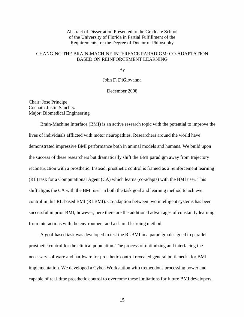
Brain-Machine Interface (BMI) is an active research topic with the potential to improve the

lives of individuals afflicted with motor neuropathies. Researchers around the world have

demonstrated impressive BMI performance both in animal models and humans. We build upon

the success of these researchers but dramatically shift the BMI paradigm away from trajectory

reconstruction with a prosthetic. Instead, prosthetic control is framed as a reinforcement learning

(RL) task for a Computational Agent (CA) which learns (co-adapts) with the BMI user. This

shift aligns the CA with the BMI user in both the task goal and learning method to achieve

control in this RL-based BMI (RLBMI). Co-adaption between two intelligent systems has been

successful in prior BMI; however, here there are the additional advantages of constantly learning

from interactions with the environment and a shared learning method.

A goal-based task was developed to test the RLBMI in a paradigm designed to parallel

prosthetic control for the clinical population. The process of optimizing and interfacing the

necessary software and hardware for prosthetic control revealed general bottlenecks for BMI

implementation. We developed a Cyber-Workstation with tremendous processing power and

capable of real-time prosthetic control to overcome these limitations for future BMI developers.

16

The RL-based BMI (RLBMI) was demonstrated in three rats for a total of 25 brain-control

sessions. Performance was quantified with task completion accuracy and speed in an

environment where difficulty increased over time. All subjects achieved control significantly

above chance over 6-10 sessions without the disjoint re-training required in other BMI.

Traditional analysis methods illustrated a representation of prosthetic actions in the rat’s

neuronal modulations. Additionally the CA’s contributions to control and the cooperation of the

rat and CA were extracted from the RLBMI network. The co-evolution of control is an impetus

to future development.

The RLBMI was motivated by overcoming the need for BMI user movements. This goal

was achieved with the additional benefits of facilitating more rapid mastery of prosthetic control

and avoiding disjoint retraining in chronic BMI use. Finally, this architecture is not restricted to a

particular application or prosthetic but creates an intriguing general control framework.

17

CHAPTER 1 INTRODUCTION

Problem Significance

The number of patients suffering from motor neuropathies is tremendous and growing.

Traumatic spinal cord injury is suffered by approximately 11,000 Americans per year [1].

Approximately 550,000 Americans survive a stroke each year, with a significant portion

suffering motor control deficits [2, 3]. Tragically, the current wars in Iraq and Afghanistan are

increasing the number of amputees – Iraq’s wounded soldiers requiring major amputation(s)

numbered 500 as of January 2007 [4]. Neuro-degenerative diseases such as amyotrophic lateral

sclerosis (ALS) and muscular dystrophy (MD) also affect approximately 5,000 and 500 new

patients respectively each year [5, 6]. This large population could all benefit from prosthetic

technologies to replace missing limbs or restore muscle control and function. In fact, in some

cases (e.g. ALS) these technologies are necessary to sustain life.

Brain-Machine Interface Overview

Brain-Machine Interface (BMI) is an active research topic1 with the potential to improve

the lives of individuals afflicted with motor neuropathies. Additionally, BMI has potential for

augmenting natural human motor function and advancing military technology. Conceptually, a

BMI creates a connection between an user’s neural activity and an external device (e.g. cursor,

robot, wheelchair, and function electrical stimulators (FES) [7]) to facilitate device control. The

most common approach for BMI is to find functional relationships between neuronal activity and

goal directed movements in an input-output modeling framework. Figure 1-1 shows a supervised

learning (SL) based BMI system for controlling a robotic arm which represents this common

approach. The three main components of the BMI are neural signal processing and the control

1BMI is also known as brain-computer interface (BCI), human-machine interface (HMI), and neural prosthetics.

18

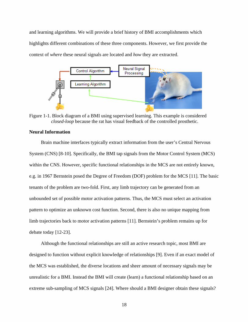
and learning algorithms. We will provide a brief history of BMI accomplishments which

highlights different combinations of these three components. However, we first provide the

context of where these neural signals are located and how they are extracted.

Figure 1-1. Block diagram of a BMI using supervised learning. This example is considered

closed-loop because the rat has visual feedback of the controlled prosthetic.

Neural Information

Brain machine interfaces typically extract information from the user’s Central Nervous

System (CNS) [8-10]. Specifically, the BMI tap signals from the Motor Control System (MCS)

within the CNS. However, specific functional relationships in the MCS are not entirely known,

e.g. in 1967 Bernstein posed the Degree of Freedom (DOF) problem for the MCS [11]. The basic

tenants of the problem are two-fold. First, any limb trajectory can be generated from an

unbounded set of possible motor activation patterns. Thus, the MCS must select an activation

pattern to optimize an unknown cost function. Second, there is also no unique mapping from

limb trajectories back to motor activation patterns [11]. Bernstein’s problem remains up for

debate today [12-23].

Although the functional relationships are still an active research topic, most BMI are

designed to function without explicit knowledge of relationships [9]. Even if an exact model of

the MCS was established, the diverse locations and sheer amount of necessary signals may be

unrealistic for a BMI. Instead the BMI will create (learn) a functional relationship based on an

extreme sub-sampling of MCS signals [24]. Where should a BMI designer obtain these signals?

19

The physiological connections of the MCS are established. There are interconnections

between three major MCS areas: the cerebral cortex, cerebellum, and basal ganglia [25, 26]. The

cerebral cortex has descending connections to the cerebellum, basal ganglia, and thalamus. The

cerebellum and basal ganglia both reciprocally connect to cerebral cortex via the thalamus.

Based on anatomical evidence, it was postulated that the cortex functions as a statistically

efficient representation of system state (e.g. controlled limb), the basal ganglia evaluate rewards

for each state, and the cerebellum contains internal models to predict state transitions [26].

Exiting the brain, there are two major projections to the motor neurons: the ventromedial

and lateral systems. Both systems contain at least one projection from the cortex and brainstem

[25]. The ventromedial system contains multiple tracts: vestibulospinal (vestibular system →

posture & balance), reticulospinal (reticular formation → coordinated movements), and

tectospinal (superior collicus → originating movements to visual stimuli). The lateral system

contains two major tracts: rubrospinal (red nucleus → distal musculature movement) and

corticospinal (cortex → voluntary movements).

Since most BMI are designed to mimic voluntary movements, it is logical to focus on the

corticospinal tract. Primary motor cortex (MI) neurons account for 30% of the information2

passed through the corticospinal tract [27], to anterior (α and γ) motor neurons in the spinal cord

[25]. Anterior motor neurons control muscle spindle activations. Coordinated motor neuron

activity will ultimately actuate the limb. However, the MI-to-motor mapping is not static [28,

29]. Motor map reorganization could represent skill learning and provide a mechanism for skill

memory [28, 30]. Alternatively, the reorganization could represent changes in other MCS

components which effectively changed the relationship of MI to the motor output.

2 Other sources of information for corticospinal tract: 30% from a combination of dorsal premotor (PMd), ventral premotor (PMv), and supplementary motor (SMA); 40% from somatosensory cortex.

20

Neural Signal Recording Techniques

Neural signals can be acquired from the MCS through a variety of techniques depending

on the control application. Groups are beginning to investigate near infrared spectroscopy

(NIRS), magneto encephalography (MEG) [31], and functional magnetic resonance imaging

(fMRI) [32, 33] for BMI; however, the low temporal resolution and current recording equipment

limits clinical applicability of these technologies. Neural signals are commonly recorded with

electrocorticographic (EEG), electroencephalographic (ECoG), or microelectrode arrays (capable

of recording local field potentials (LFP) or single-unit activity). These technologies have

advantages and disadvantages in spatio-temporal resolution and patient invasiveness [8, 34, 35].

There is active and successful BMI research utilizing other neural signals including: EEG

[36, 37], ECoG [38-40], and LFP [35, 41, 42]. However, prior literature suggests that single units

(recorded with microelectrodes) are necessary for complex motor control [34, 43-47].

Additionally, there is experimental and neurophysiological support for the theory that the brain

utilizes rate coding [8, 48-50]; firing rate (FR) can be estimated from single-unit activity. The

next section reviews historical BMI achievements using single-unit rate coding.

A Short History of Rate Coding BMI

BMI technology was pioneered in the 1980s by Schmidt [51], when he showed first that

cortical electrodes could maintain recordings in monkeys for over three years and the animals

could modulate neural firing to control a prosthetic with less than a 45% reduction in information

transfer. Specifically, the bit transfer rate from modulations to prosthetics was only 45% less

than the bit transfer rate from joystick (which the monkey physical moved) to prosthetic.

Significant BMI contributions were then made by Georgopoulos’ group [52-55], most notably

the population vector algorithm (PVA) [53]. In a standard center-out reaching task, they found a

preferred direction of maximal FR for each neuron and a tuning function specifying FR in the

21

non-preferred directions. The PVA used vector summation of the tuning functions of all recorded

neurons to map FR to hand trajectory [54]. PVA removes some neural FR variability which can

be problematic for BMIs.

Chapin’s group advanced the BMI paradigm design by incorporating a robotic arm that the

animal not only controlled, but also directly interacted with [56]. The paradigm used principal

components analysis (PCA) of the neural signal and recurrent artificial neural networks (rANN)

to control a robotic arm. This arm delivered water rewards to the animal; after repeated trials the

animal ceased limb movements.

Kennedy published the first results on invasive BMI for a human in 2000. This BMI

utilized rate coding for 2D cursor control in patients with ALS. Control was based on FR

modulation of two recorded neurons. After five months the patient claimed to be thinking of

‘moving the cursor’ [57]. However, due to ALS complications, this experiment did not

demonstrate the expected speed increase over noninvasive BMI.

Nicolelis’s multi-university collaboration demonstrated real-time robotic arm control in

primates in 2000 [49]. They showed that multiple cortical areas and hemispheres (rather than

only contra lateral MI) are useful for BMI control [58]. However, they found that MI neurons,

compared to other brain areas independently, were the ‘best predictors for all motor variables.’

[59] Introducing a robotic arm illustrated an interesting result: animals incorporated the robot’s

dynamics into their own internal MCS models [59]. The group also investigated ‘mixture-of-

experts’ BMI techniques. The nonlinear mixture of competitive linear models (NMCLM)

technique was more accurate than either a moving average (MA) or tap-delay neural network

(TDNN); however, due to data limitations inherent in multiple model BMI, it could not

outperform a recursive multilayer perceptron (RMLP) [60].

22

Taylor, Schwartz and Tillery collaboration illustrated two important BMI issues [61-64].

First, biofeedback to the patient approximately doubled brain control accuracy in a 3D center-out

task [64]. Taylor also include a robotic arm in the loop [65] with similar results to [59]. Second,

this group continued to train the BMI during brain control, allowing the algorithms learned from

their own outputs. This ‘co-adaptive’ system adjusts the neural tuning function [54] in the PVA

as the animal adjusted its own neural modulation patterns.

Serruya et al. showed ‘instant’ 2D cursor control from 7-30 neurons in monkeys using

linear filters that are updated throughout the brain control phase after a brief training

initialization [66]. One of the monkeys in this study was able to achieve brain-controlled cursor

movement at similar speeds to joystick controlled movement.

Shenoy et al. trained maximum likelihood decoders for reconstructing monkey’s arms

movements with offline data from parietal reach region (PRR) [67]. Although there was arm

movement in the original recordings, only neural data from the movement planning stage was

used. They reported 90% task performance with only 40 neurons [67]. It is unclear how this

performance may change with biofeedback to the animal or if the neural planning was not for a

well-practiced motion. However, they illustrate significant planning in PRR.

Musallam et al. also investigated novel BMI control strategies outside of MI. The firing

rates of neurons from PRR and PMd were used to control goal-based rather than trajectory-

based BMIs [68]. Neural response databases were constructed during training (updated in brain-

control) and used during brain control to decode the monkey’s intent. This architecture was

interesting because it assigns a specialized, subordinate controller to handle details of achieving

tasks – the BMI only discriminates between tasks. Reinforcement learning researchers have

proposed a similar hierarchical models, although not in a BMI framework [69]. The control

23

model selects a goal; the lower model uses a set of trajectory primitives to reach the goal [69,

70]. Todorov et al. have also suggested this hierarchical strategy is utilized in the human MCS

for optimal feedback control [71].

Si, Hu, He, and Olson did not focus on a particular MI area (e.g. forelimb), instead they

sample the neck, forepaw, and shoulder in a two lever choice task [72]. Support Vector Machines

(SVM) classify different rat actions using Neural Activity Vectors (NAV), which are arrays of

firing rates defined relative to the start of behavioral trials. Unlike many BMI, there were no

restrictions on the rat’s behavior and no trajectory data was used [72]. The group is investigating

PCA of NAV as a feature extraction preprocessing for SVM and Bayesian classifiers [73]. Their

goal is to directly interfacing the prosthetic into the rat’s world – the BMI will classify actions

which will move the rat (on a mechanical cart) towards a reward location [74].

Kipke’s group advances Taylor’s and Serruya’s research by creating naïve BMI systems

which do not require patient motion or prior motor training. Kalman filters[75] are used to map

neural ensemble FR to cursor position; the filters are trained with block estimation in 10 prior

(brain-controlled) trials. Within 3 days, rats were able to perform a 1D cursor control task above

chance levels with no prior training and no desired signal [76].

In 2006, SP Kim et al. comprehensively investigated linear and non-linear BMI models for

optimal performance and generalization [77]. Non-linear models, while useful for rest periods of

motion, were not significantly superior to simple linear models for continuous motion tasks. The

NMCLM had higher performance because each expert specialized on one motion segment [77].

This work illustrated a weakness of mixture-of-experts models, determining switching times and

extra parameters to train.

24

HK Kim et al. developed an BMI control technique where some of the system’s

intelligence is transferred from the control algorithm to the robotic arm [78]. Weighting the

contribution of the neural decoding algorithm (70%) and robotic sensor collision detection

(30%), the group achieved a performance improvement of ‘seven-fold’ above neural decoding

alone [78]. This novel approach enhances the BMI via direct feedback.

Cyberkinetics reported human clinical trials of the BrainGate BMI system [50]. The

system facilitated 3D (two Cartesian and one click dimension) cursor control. The patient was

able to use email or operate remote controls while engaged in other activities [50]. The BMI uses

supervised learning; however, the desired signal was a technician’s cursor movement. Rapid

learning was demonstrated in videos at various conferences. Additionally the subject (without

prior training) could control a prosthetic hand to grip and release within a few trials [50].

Several groups are adding more biological inspiration to BMI research, e.g. incorporating

biomechanical models of the user’s arm [79, 80]. These models allow the BMI to map neural

activity to muscle activation without the recording uncertainties and noise of EMG. There are SL

generalization advantages gained using these models. It is feasible to train a BMI over the

complete range of muscle activations (0:1); training over the range of possible endpoint or joint

positions is much more difficult (if possible) in an unconstrained motion paradigm [80].

Additionally, the models reveal that the previously reported ‘high correlation’ of neural signals

to both kinematic and dynamic arm variables [81, 82] may not be an intrinsic feature of MI

coding , rather the correlation is a function of paradigm design that can be avoided [79].

Common Rate Coding BMI Themes and Remaining Limitations

The prior three decades of BMI research created some incredible technological advances

and gave hope to many who suffer from motor neuropathies. Each research group created a

particular BMI control application (e.g. cursor control, robot self feeding, task selection) with

25

different learning algorithms; hence, their contributions were different. However, there are some

shared themes that appear across the different historical approaches in the prior section.

• Primary motor cortex provides useful information for BMI trajectory reconstruction • Both trajectory-based and goal-based BMI have been achieved through rate-coding • Biofeedback can dramatically improve BMI performance in brain-control • Co-adaptation can also improve BMI performance in brain-control • Biologically inspired architectures can reduce training and improve control

The next generation of BMI should exploit this existing knowledge base and incorporate

these features to maximize control performance. However, there are also common problems that

appear (or would appear in implementation) across the different approaches in the prior section:

1. Finding an appropriate training signal in a clinical population of BMI users 2. Maintaining user motivation over length BMI training to master control 3. Relearning control whenever the neural signal or environment is non-stationary Designers must address these implementation issues to advance the state of the art. The last

section focused on the positive aspects of prior BMI, these implantation issues are described in

the next subsections.

Finding an Appropriate Training Signal in a Clinical Population of BMI Users

An aspect that is dismissed by many designers has been the clinical feasibility of their

training signal. Trajectory-based BMI find functional relationships between neuronal activity

and goal directed movements in an input-output modeling framework. A tremendous amount of

information can be concentrated in the error between the user’s movements and the BMI output;

hence, algorithmic design is greatly simplified. These BMI are very effective for users without

motor neuropathies in a laboratory setting. However, the population with motor neuropathies

typically does not have the ability to move; hence they could not train these BMI.

A few groups have created an engineering solution for this problem which replaces the

user’s movements with a technician’s movement [50]. The user is simply asked to attend to the

26

technician’s movements. While this represents a positive step for introducing BMI into the

clinic, it creates another set of problems. In laboratory experiments, the healthy user modulations

neuronal activity, the information passes through the nervous system (with some conduction

delays), and then the limb moves. The SL BMI makes a variety of assumptions (e.g. a linear

filter can represent all dynamics of the MCS) to map between neural activation and limb

movement. Adding a technician fundamentally changes the paradigm. The user must now

observe the movements (with sensory delays) and then imagine a similar movement and/ or

predict future movements. This user-to-technician sensory interpretation introduces another

source of error which can degrade the BMI approximation; hence degrade possible performance.

Ideally, sophisticated and well-trained BMI algorithms can overcome these additional

layers of uncertainty in the neural- to-movement mapping. However, this solution still raises the

issue of clinical feasibility – Should a BMI be dependant on availability of a highly-skilled

technician? It is unrealistic to require a technician to train a BMI to achieve all Activities of

Daily Life (ADL) [83-85]. Even allowing both strong assumptions that the BMI can create an

accurate mapping and a constantly available technician, the user still lacks independence and the

ability to learn from interactions with the environment.

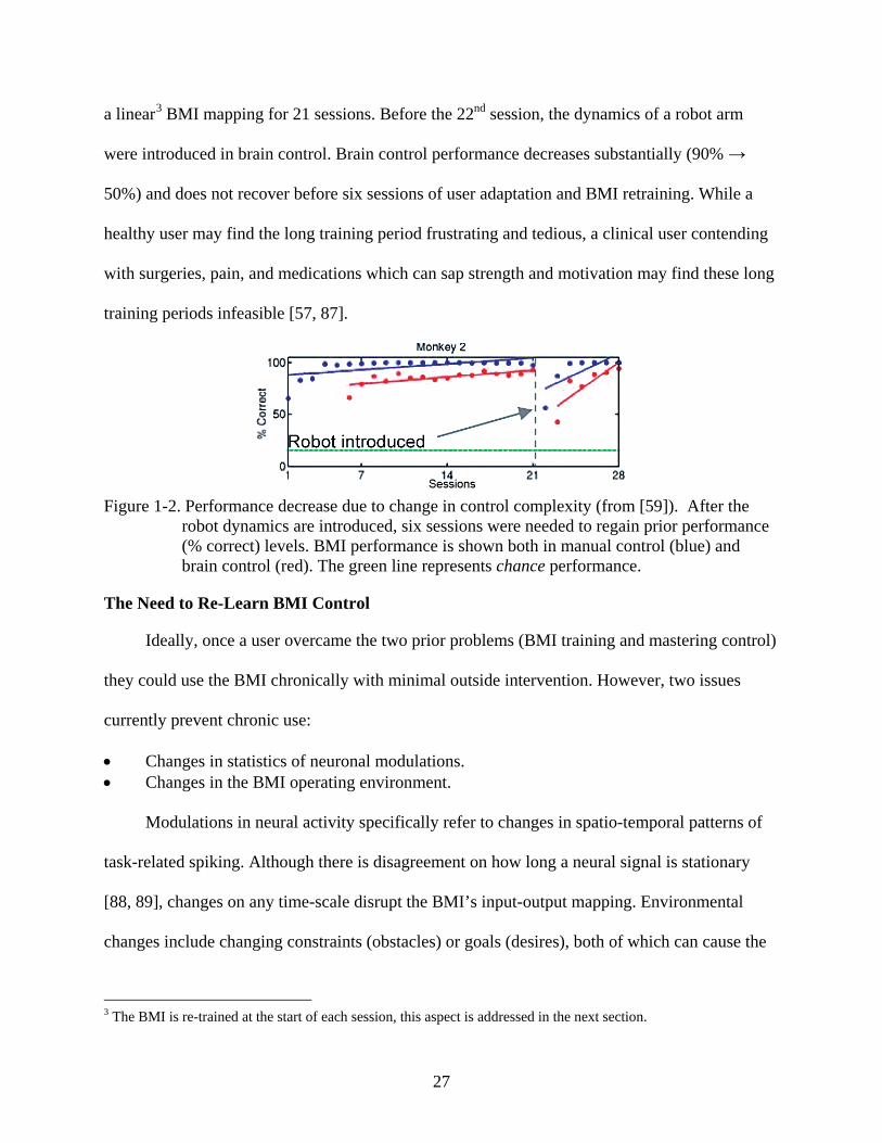
Maintaining User Motivation over Lengthy BMI Training to Master Control

The time needed to master BMI control increases as the control tasks become more

complicated. For example, when the dynamics of an external device are introduced or task

difficulty increases, the user must learn this more a more complex control scheme and

performance metrics initially decrease [50, 59, 65, 86]. It may require multiple sessions (hours to

days) of user training to return to the prior level of mastery in control. An example from

Carmena et al. is shown in Figure 1-2 where a monkey was engaged in 2D cursor control through

27

a linear3 BMI mapping for 21 sessions. Before the 22nd session, the dynamics of a robot arm

were introduced in brain control. Brain control performance decreases substantially (90% →

50%) and does not recover before six sessions of user adaptation and BMI retraining. While a

healthy user may find the long training period frustrating and tedious, a clinical user contending

with surgeries, pain, and medications which can sap strength and motivation may find these long

training periods infeasible [57, 87].

Figure 1-2. Performance decrease due to change in control complexity (from [59]). After the

robot dynamics are introduced, six sessions were needed to regain prior performance (% correct) levels. BMI performance is shown both in manual control (blue) and brain control (red). The green line represents chance performance.

The Need to Re-Learn BMI Control

Ideally, once a user overcame the two prior problems (BMI training and mastering control)

they could use the BMI chronically with minimal outside intervention. However, two issues

currently prevent chronic use:

• Changes in statistics of neuronal modulations. • Changes in the BMI operating environment.

Modulations in neural activity specifically refer to changes in spatio-temporal patterns of

task-related spiking. Although there is disagreement on how long a neural signal is stationary

[88, 89], changes on any time-scale disrupt the BMI’s input-output mapping. Environmental

changes include changing constraints (obstacles) or goals (desires), both of which can cause the

3 The BMI is re-trained at the start of each session, this aspect is addressed in the next section.

28

user to modify known or develop new control schemes (tasks). The reason these two changes can

be so disruptive is due to the way a BMI typically learns.

Learning the input-output BMI mapping

Often described as “decoding,” [90] the process of discovering the functional mapping

between neuronal activity and behavior has generally been implemented through two classes of

learning: supervised [91] and unsupervised [92]. An unsupervised learning (UL) approach finds

structural relationships in the data [93] without requiring an external teaching signal. A

supervised learning (SL) approach uses kinematic variables as desired signals to train a

(functional) regression model [77] or more sophisticated methods [94]. Both approaches seek

spatio-temporal correlation and structure in the neuronal activity relative to control in the

environment and fix model parameters after training. Fixing parameters provides a memory of

the past experiences for future use, but suffers from the problem of generalization to new

situations. Multiple groups have shown the negative consequences of disrupting this mapping in

both monkey [58] and human [50, 95] BMI users. In order to overcome either neuronal or

environmental changes, the BMI must re-learn this mapping as described next.

Retraining the BMI mapping

BMI developers typically use a retraining period before each use to overcome these issues.

Similar to technician training, this is an engineering solution to a problem which creates two

new problems. First, every new control session (day) has to be preempted (delayed) by the

collection of training data and the time required for BMI training. This retraining may or may not

require a technician (Problem 1) but definitely will induce delay before control. Depending on

the BMI, this delay may range from inconvenient (the user must wait while the algorithm trains)

to exhausting (the user must provide many examples of training data; the user must remain both

motivated and physically active).

29

Second, BMI are trained to map many neural inputs to few outputs in order to minimize a

cost function. If the networks are reinitialized, it is possible that the BMI will learn a mapping

that achieves similar cost (similar local minima in the cost manifold as the prior day) via a

different combination of inputs. This reorganization of the map can effectively erase prior

knowledge that the user (and BMI) had accumulated about using the device. The repeated loss of

knowledge that may happen prior to every control session may explain why users are slow to

master BMI control (Problem 2).

Other Reports Confirming these Problems in BMI

These significant problems from the BMI literature have also been identified by other

panels of experts. In the ‘Future Challenges for the Science and Engineering of Learning’, a

panel of 20 international researchers concludes that the most pressing 'open problem in both

biological and machine learning' as the requirement of a human designer and supervised learning

[96]. Additionally, a World Technology Evaluation Center (WTEC) report reviewing the

international state of the art in Brain-Computer interfaces identified the specific need to develop

adaptive devices which are modulated by feedback [97]. The WTEC report also criticized current

neural interface for requiring subjective human intervention. Therefore, any attempt to advance

the state-of-the-art in neuroprosthetic design must overcome the above mentioned issues.

Contributions

We incorporate the positive insights of prior BMI research, but do not attempt to compete

with existing SL techniques, i.e. we have no intention to more accurately reconstruct center-out

trajectories. Such improvements would be technologically interesting but are not the focus of

this research. Instead, we will substantially advance the state of the art by shifting the BMI

design philosophy. Rather than engineering ‘work-arounds’ for SL limitations, we shift to a

Reinforcement Learning (RL) based BMI architecture (RLBMI). This novel design creates a

30

BMI architecture which both facilitates user control and directly addresses the clinical

implementation problems identified in the prior sections.

The RLBMI learns from interactions with the environment rather than a supervisor’s

training signal. The learning philosophy eliminates (or reduces) the need for a technician to use

the BMI. Learning from the environment also creates the opportunity for the BMI to learn

continuously, even in brain-control. Specifically, both the user and the BMI are learning together

to complete tasks. This idea is called co-adaptation; it has been suggested to be a critical design

principle for the next generation BMIs by BMI researchers like Kipke [98] and Taylor [65, 99]

(reviewed in the History of Rate Coding section) and BCI researchers like Millan and Wolpaw

who both work with EEG. In Milan’s research the user is interacting with a virtual keyboard; as

the user tried to select a letter the BCI continues to split the keyboard so that the user has fewer

letters available until there is only one left (the selected letter) [100]. Effectively this makes the

task easier for the user over time. Wolpaw’s research group at the Wadsworth center is interested

in automated feature and channel selection and also automated gain selection for cursor control

from those channels [101]. While all these researchers understand the potential of co-adaptation,

it has not been fully realized in the constraints of supervised learning architectures.

Synergistic co-adaptation in the RLBMI can reduce the amount of time necessary for a

user to master BMI control. This reduced training time would be enabling to the user – they

avoid wasting valuable time and limited energy. Potentially this creates a positive feedback

where the user actively controls the BMI for longer periods; then the BMI has more opportunity

to adapt to the user over these periods to improve performance. Improved performance

encourages even longer periods of user control, which gives the BMI more time to learn, etc.

31

Finally, the ability of the RLBMI to co-adapt allows it to retain past experience while still

adapting to changes in the user’s neural modulations. This crucial feature allows the RLBMI to

be used day-after-day without retraining – introducing continuity in BMI control. Furthermore,

the RLBMI can co-evolve to learn new tasks based on interactions with the environment instead

of disjoint retraining sessions. Again, co-adaption may facilitate more rapid mastery of the new

control tasks.

Overview

This dissertation is organized into seven chapters – each highlighting a major theme of

developing (chapters 2-4) and validating (chapters 5-6) this novel BMI architecture. The second

chapter discusses the necessary structural changes in BMI design to exploit the advantages of

RL. The third chapter discusses the behaviorist concepts that are necessary to develop an

appropriate animal model to validate the RLBMI. The fourth chapter focuses on the engineering

challenges in implementing closed-loop RLBMI control in the animal model.

Chapter five includes the training and overall performance of the closed-loop and co-

adaptive RLBMI. It focuses on RLBMI performance from an engineering perspective. The sixth

chapter analyzes RLBMI performance at a lower level of abstraction – providing both algorithm

and neurophysiological quantifications of the co-evolution of the system. The final chapter

summarizes the significant and novel contributions to the field of BMI, implications of the

RLBMI architecture, and future developments and integration.

32

CHAPTER 2 CHANGING THE LEARNING PARADIGM

The Path to Developing a Better BMI

Since the first Terminator movie, I have been intrigued by learning computers even if they

seemed a distant sci-fi fantasy. Surprisingly, after a series of classes in adaptive filters design and

neural networks, this power was now at my fingertips. Once I had finally grasped the

mathematics, I could code my own algorithms which learned to solve problems. Furthermore, I

could build on established BMI solutions. Initially I ignored the broad spectrum of potential

implementation issues due to the stationarity assumption in BMI (contributions 2 and 3). Instead,

I focused on the clear BMI design flaw of requiring a desired signal (movements) to train the

controller from a clinical population without this capability. Now all I had to do was code a

solution… blindly optimistic that I could advance decades of BMI design in a Matlab m-file.

Hacking away at the Problem

The combination of optimism and decent programming ability generated many different

BMI algorithms rooted in the supervised learning and trajectory reconstruction concepts

reviewed in the prior chapter. Typically they applied some clever hack such as delaying a desired

signal to make it available at prescribed times or synthesizing a desired signal based on the

current prosthetic trajectory. These algorithms were effective in a narrow sense overcame the

requirement for a desired signal. Ultimately these hacks would introduce problems in other areas

(e.g. causality) and were failures because they did not critically consider the entire BMI.

Initially, I met these failures by redoubling my efforts without changing my mindset. Each new

algorithm advanced my programming ability and I had gained access to a computing cluster –

this led to increasingly complex algorithms. These typically took longer to code, train, and

33

analyze but this increased investment did not create the expected returns because they still didn’t

properly consider the problem.

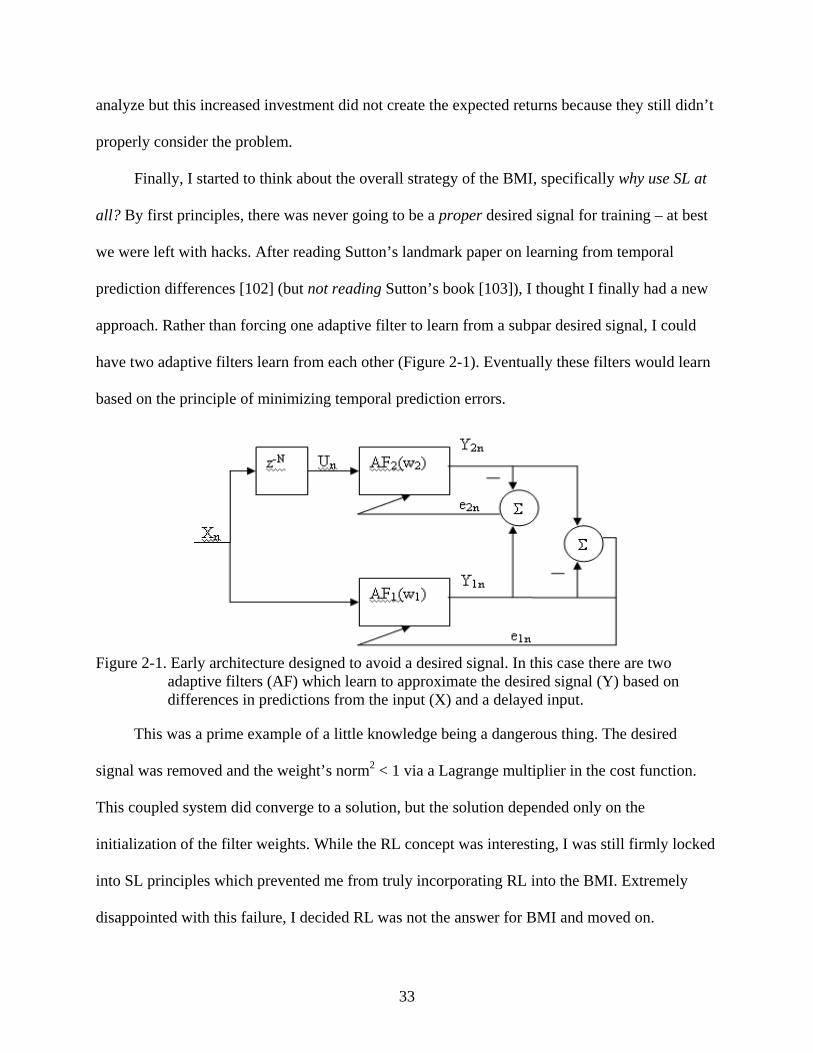
Finally, I started to think about the overall strategy of the BMI, specifically why use SL at

all? By first principles, there was never going to be a proper desired signal for training – at best

we were left with hacks. After reading Sutton’s landmark paper on learning from temporal

prediction differences [102] (but not reading Sutton’s book [103]), I thought I finally had a new

approach. Rather than forcing one adaptive filter to learn from a subpar desired signal, I could

have two adaptive filters learn from each other (Figure 2-1). Eventually these filters would learn

based on the principle of minimizing temporal prediction errors.

Figure 2-1. Early architecture designed to avoid a desired signal. In this case there are two

adaptive filters (AF) which learn to approximate the desired signal (Y) based on differences in predictions from the input (X) and a delayed input.

This was a prime example of a little knowledge being a dangerous thing. The desired

signal was removed and the weight’s norm2 < 1 via a Lagrange multiplier in the cost function.

This coupled system did converge to a solution, but the solution depended only on the

initialization of the filter weights. While the RL concept was interesting, I was still firmly locked

into SL principles which prevented me from truly incorporating RL into the BMI. Extremely

disappointed with this failure, I decided RL was not the answer for BMI and moved on.

34

Principled Solutions in the Input Space

Dissatisfied with the hacks and associated failures, I began to lean more heavily on the

biomedical side of my engineering education. Through physiology and clinical anatomy I was

able to gain a more intimate understanding of the human MCS. Even though it does not address

the desired signal issue, I investigated whether the recorded neural signals could be preprocessed

in a biologically sensible way that would also improve BMI performance [104]. Specifically we

used population averaging – a biologically-inspired technique based on spatial constraints and

neuronal correlation. Theoretically, all neurons have firing variability (one could label this noise

but should be cautious) but those neurons within the same cortical column are all sending the

same message1. Therefore variability (loosely noise) can be reduced by averaging across all

members of a cortical column.

The neural data was organized into three different preprocessing configurations that will

modify the functional mapping between neural activity and behavior (number of filter inputs

listed in parenthesis):

• AN – All sorted neurons (42) • PA – Population averaging (23) • MV – Minimum binning variance (23)

The AN configuration uses standard BMI assumptions and is considered the benchmark.

The PA configuration averages individual neurons which meet spatial and temporal correlation

requirements of being in a cortical column [104-106]. The MV configuration is organized to

create maximal reduction in FR variance for each quasi-column and serves a control against PA.

In a test dataset, an estimated lever position is reconstructed using the optimal MSE

weights. A range of thresholds (applied after the Wiener Filter (WF)) is tested to find the 1 There is conflicting research that the cortical column [104] is a ‘structure without a function’ [105]. We only use the structure and do not make assumptions about what the sent message may be.

35

maximum model accuracy [104]. A two-sample Kolmogorov-Smirnov [K-S] test (95%

significance) is used to compare all filter outputs with the AN WF.

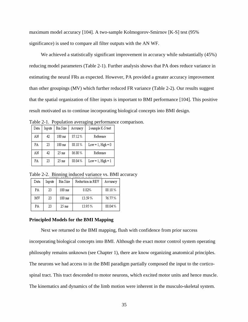
We achieved a statistically significant improvement in accuracy while substantially (45%)

reducing model parameters (Table 2-1). Further analysis shows that PA does reduce variance in

estimating the neural FRs as expected. However, PA provided a greater accuracy improvement

than other groupings (MV) which further reduced FR variance (Table 2-2). Our results suggest

that the spatial organization of filter inputs is important to BMI performance [104]. This positive

result motivated us to continue incorporating biological concepts into BMI design.

Table 2-1. Population averaging performance comparison.

Table 2-2. Binning induced variance vs. BMI accuracy

Principled Models for the BMI Mapping

Next we returned to the BMI mapping, flush with confidence from prior success

incorporating biological concepts into BMI. Although the exact motor control system operating

philosophy remains unknown (see Chapter 1), there are know organizing anatomical principles.

The neurons we had access to in the BMI paradigm partially composed the input to the cortico-

spinal tract. This tract descended to motor neurons, which excited motor units and hence muscle.

The kinematics and dynamics of the limb motion were inherent in the musculo-skeletal system.

36

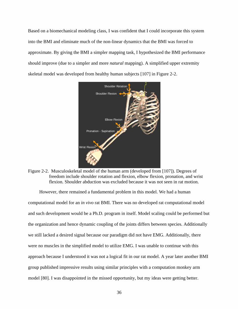
Based on a biomechanical modeling class, I was confident that I could incorporate this system

into the BMI and eliminate much of the non-linear dynamics that the BMI was forced to

approximate. By giving the BMI a simpler mapping task, I hypothesized the BMI performance

should improve (due to a simpler and more natural mapping). A simplified upper extremity

skeletal model was developed from healthy human subjects [107] in Figure 2-2.

Shoulder Rotation

Shoulder Flexion

Elbow Flexion

Pronation - Supination

Wrist Flexion

Figure 2-2. Musculoskeletal model of the human arm (developed from [107]). Degrees of

freedom include shoulder rotation and flexion, elbow flexion, pronation, and wrist flexion. Shoulder abduction was excluded because it was not seen in rat motion.

However, there remained a fundamental problem in this model. We had a human

computational model for an in vivo rat BMI. There was no developed rat computational model

and such development would be a Ph.D. program in itself. Model scaling could be performed but

the organization and hence dynamic coupling of the joints differs between species. Additionally

we still lacked a desired signal because our paradigm did not have EMG. Additionally, there

were no muscles in the simplified model to utilize EMG. I was unable to continue with this

approach because I understood it was not a logical fit in our rat model. A year later another BMI

group published impressive results using similar principles with a computation monkey arm

model [80]. I was disappointed in the missed opportunity, but my ideas were getting better.

37

Motion Primitives in the Desired Trajectory

Although we could not incorporate the skeletal model in Figure 2-2 into the BMI mapping,

this model was very useful for another idea which had been percolating. We hypothesized that a

set of movemes (aka motion primitives) could be extracted from biological motion [108] and

wanted to build on the work of prior movemes researchers (see Chapter 1). In the absence of real

motion, we created bio-mechanically realistic motions. Trajectories were based on a rat

behavioral experiment [109]. The motion is generated via inverse dynamics optimization [110,

111] of a minimum commanded torque change cost function found in biomechanical modeling

[112, 113] via a general-purpose musculoskeletal modeling system [114] (more details in [108]).

As proof-of-concept we tested movemes ability to reconstruct these trajectories.

There are physiological relationships between muscle force generation and both muscle

length and muscle velocity [25, 82, 111, 115]. Identical muscle activations will create different

muscle forces depending on these two relationships. Muscle lengths and velocities are

determined based on the angular positions and velocities of the joints that the muscle spans. The

muscle’s moment arm across a joint is determined by the ratio of change in muscle length to

change in joint angle. The torque produced at a joint is the sum of muscle forces multiplied by

their moment arms across that joint. These three physiological relationships show that joint

angle2 relationships are important and may serve as a descriptor of different arm states. Hence

we extract features from the joint angle space which correspond to our definition of movemes.

We defined these features by the relationship between the current and next sets of joint

angles – the features are shown over the course of a motion in Figure 2-3. The features provide

joint angular velocity and also position can be inferred based on initial conditions. Machine

2 All joints angles are shown in Figure 2-2. The joint-angle space comprises five dimensions.

38

learning techniques were employed to partition the feature space. Without a priori knowledge of

the correct number (or existence) of movemes, only use clustering error is a guide to how to

group the features. Two approaches were used to find an optimal number of 42 clusters [108].

Figure 2-3. Motion features and cluster centers in joint angle space. Most proximal axes of joint

angle space are shoulder flexion (vsf), elbow flexion (vef) and wrist flexion (vwf). Small circles are features; larger X-filled circles are cluster centers (potential movemes)

The optimal cluster centers (see Figure 2-3) are tested for their utility in reconstruction of

the synthetic motion. Each center is added to the initial joint angle vector to create estimates of

the next joint angle vector. The estimate with least error relative to the next true joint angle

vector is selected. Reconstruction then proceeded recursively, but there was no rigid time

structure in cluster selection [108]. The optimal cluster set that best parameterized the joint angle

space for synthetic trajectory reconstruction was less than 10% of the feature set size. We

hypothesized the clusters were potentially movemes but cautioned that neural correlation was

necessary to validate this idea. In subsequent (unpublished) analysis, three issues prevented

investigating this correlation. The computational model species mismatch and rat motion timing

variability would both introduce errors in the synthetic trajectories. Finally, the 1 ms time

resolution of these movemes is problematic (processing, generalization, and storage) in an ANN.

Despite these problems which ultimately prevented this type of movemes investigation,

there was a very beneficial by-product from the research. Our paper was accepted to the World

39

Congress on Computer Intelligence in Vancouver. I presented the research [108] and received

positive but non-specific feedback. Between other BMI talks, I had free time and saw talks on

Artificial Intelligence (AI) in video games. I was impressed what the AI could do both as an

algorithm designer and a gamer. All of the designers had used some variant of RL to train their

AI. At the time, I was delving further into operant conditioning principles to more effectively

train the rats in the BMI model (see Chapter 3). Somewhere in my mind there was a perfect

storm of positive results from both rats and AI – suddenly RL made a lot more sense for BMI.

Reinforcement Learning Theory

The conventional RL paradigm involves two entities: the agent and the environment [103].

The agent represents an intelligent being attempting to achieve a goal. The environment

represents anything the agent cannot directly modify but can interact with. The interaction is

defined by the agent’s actions which influence the environment and the states and rewards

observed from the environment (see Figure 2-4). The agent’s actions at are defined by the

existing interface with the environment. The environment’s state st is defined as a Markov

descriptor vector [103]. After the agent completes an action, the environment provides a reward

rt+1. The agent attempts to maximize these rewards for the entire task – which is expressed as

return Rt (given in Equation 2-1) where rn is the reward earned at time n and γ is a discounting

factor (≤ 1) that controls the horizon of future rn that will be considered for the task.

The agent has no information about whether selected actions were optimal at the time they

were executed. Instead the agent follows a policy which should maximize reward. This policy is

based on the agent’s ability to estimate a value Q for the state-action pairs based on observed

rewards. The optimal Q* (given in Equation 2-2) is the expected return (Equation 2-1) In the RL

literature, one of two values (V or Q) is used depending on the paradigm. The state value (V) is

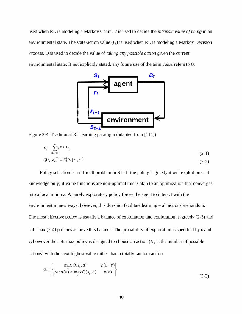
40

used when RL is modeling a Markov Chain. V is used to decide the intrinsic value of being in an

environmental state. The state-action value (Q) is used when RL is modeling a Markov Decision

Process. Q is used to decide the value of taking any possible action given the current

environmental state. If not explicitly stated, any future use of the term value refers to Q.

agent

environment

at

rt

st+1

rt+1

st

Figure 2-4. Traditional RL learning paradigm (adapted from [111])

∑∞

+=

+−=1

1

tnn

tnt rR γ

(2-1)

( ) { }ttttt asREasQ ,|, * = (2-2)

Policy selection is a difficult problem in RL. If the policy is greedy it will exploit present

knowledge only; if value functions are non-optimal this is akin to an optimization that converges

into a local minima. A purely exploratory policy forces the agent to interact with the

environment in new ways; however, this does not facilitate learning – all actions are random.

The most effective policy is usually a balance of exploitation and exploration; ε-greedy (2-3) and

soft-max (2-4) policies achieve this balance. The probability of exploration is specified by ε and

τ; however the soft-max policy is designed to choose an action (Na is the number of possible

actions) with the next highest value rather than a totally random action.

≠−

= )(),(max)()1(),(max

εε

pasQarandpasQ

ata

tat

(2-3)

41

∑

=

a

t

t

N

bsQ

asQ

t

e

eapτ

τ

),(

),(

)(

(2-4)

Equations 2-1 and 2-2 can be rewritten as Equation 2-5 which is an unbiased estimator of

the Bellman optimality equation [103] (Equation 2-6) if the policy is optimal (denoted *).

)},({),( *11 asQrEasQ tttt ++ += ππ γ (2-5)

[ ])','(max),( *

'''

'* asQRPasQ

a

ass

s

ass γ+= ∑

(2-6)

),|'( 1' aasssspP ttta

ss ==== + (2-7)

},',|{ 11' aassssrER ttttass ==== ++ (2-8)

If a perfect environmental model is known a priori, the optimal value function (Equation

2-6) can be found via Dynamic Programming (DP) [103]. However, the computational cost of

DP algorithms is exponential. A simple grid-world with 6 states and 8 actions takes less than

minutes to compute (C++, 3.4 GHz P4, 2 Gb RAM). If the only number of actions is increased

to 12, the computational time increases to ~22 hours.

Rather than assuming a complete model of the environment, Monte Carlo (MC) methods

learn optimal value functions from experience [103]. This technique relies on averaging total

rewards earned from a given state-action pair to learn the value function; assuming each state-

action pair is visited an infinite number of times, the value function converges to (Equation 2-2).

However, this method has two major limitations. First, the assumption that all state-action pairs

will continue to be visited may be difficult to satisfy due to environmental dynamics. Second,

averaging total rewards prevents value function improvement prior to the trials end.

RL provides an efficient approximation to either DP or MC technique because of its on-

line learning [103]. Additionally, RL can be used without a model of the environment where DP

cannot [103].A RL technique that utilizes ideas from both DP and MC method is Temporal-

42

Difference (TD) learning [102, 103, 116, 117]. TD learning is a boot-strapping method that uses

future value estimates to improve current value estimates. MC (Equation 2-9) and TD (Equation

2-10) learning of value functions is provided for comparison:

)],([),(),( ttttttt asQRasQasQ −+← α (2-9)

)],(),([),(),( 111 ttttttttt asQasQrasQasQ −++← +++ γα (2-10)

Using MC methods, Q is updated (Equation 2-9, α is the learning rate) using the total

return (Equation 2-1). TD methods instead update Q at the next time step (Equation 2-10). This

can greatly increase learning speed, e.g. if a low valued state-action pair is observed, Q for this

pair can be immediately updated to reduce the action’s probability in future state occurrences.

Obviously, TD learning is sensitive to the accuracy of the value function (it assumes Q(st+1,at+1)

is a good approximation of Rt+1) and may become unstable [118]. However with appropriate

parameters this TD method asymptotically converges to the optimal value function [102].

Modeling the BMI User with RL

Understanding these RL concepts is a necessary, but not sufficient condition to develop a

RL-based BMI. The problem is a common trap in analyzing the rat BMI model. The rat is

intelligent, can make movements (actions) through its motor system, and can observe the

environment (states) through its sensory system. Hence it is intuitive to model the rat with the

agent in Figure 2-4. Furthermore, considering that the rat was trained via operant conditioning it

follows that rat learning should logically be modeled with RL. This model will predict how the

rat would adapt to different schedules of reward (e.g. variable schedules, extinction) or changes

in the environment. This model would allow experiments to simulated the effects of different

operant conditioning strategies to maximize rat performance [119].

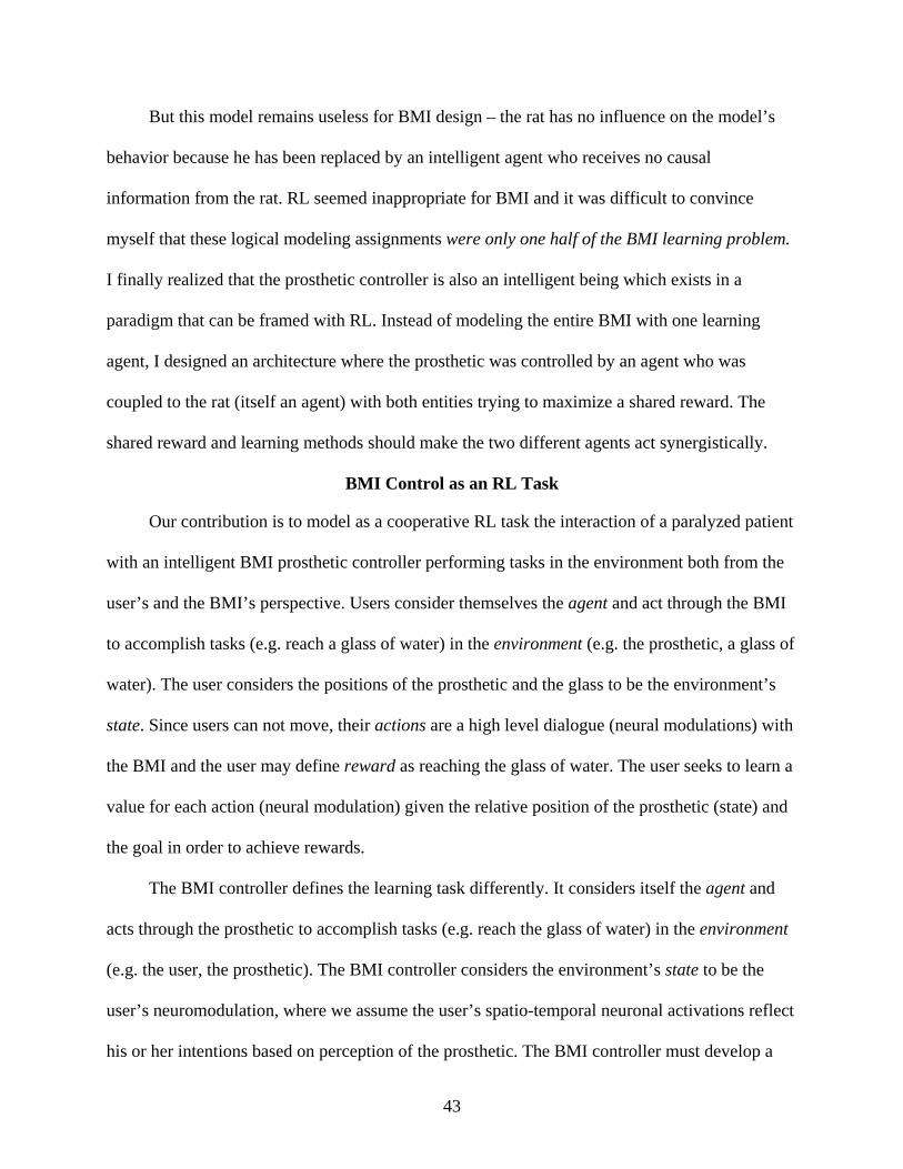
43

But this model remains useless for BMI design – the rat has no influence on the model’s

behavior because he has been replaced by an intelligent agent who receives no causal

information from the rat. RL seemed inappropriate for BMI and it was difficult to convince

myself that these logical modeling assignments were only one half of the BMI learning problem.

I finally realized that the prosthetic controller is also an intelligent being which exists in a

paradigm that can be framed with RL. Instead of modeling the entire BMI with one learning

agent, I designed an architecture where the prosthetic was controlled by an agent who was

coupled to the rat (itself an agent) with both entities trying to maximize a shared reward. The

shared reward and learning methods should make the two different agents act synergistically.

BMI Control as an RL Task

Our contribution is to model as a cooperative RL task the interaction of a paralyzed patient

with an intelligent BMI prosthetic controller performing tasks in the environment both from the

user’s and the BMI’s perspective. Users consider themselves the agent and act through the BMI

to accomplish tasks (e.g. reach a glass of water) in the environment (e.g. the prosthetic, a glass of

water). The user considers the positions of the prosthetic and the glass to be the environment’s

state. Since users can not move, their actions are a high level dialogue (neural modulations) with

the BMI and the user may define reward as reaching the glass of water. The user seeks to learn a

value for each action (neural modulation) given the relative position of the prosthetic (state) and

the goal in order to achieve rewards.

The BMI controller defines the learning task differently. It considers itself the agent and

acts through the prosthetic to accomplish tasks (e.g. reach the glass of water) in the environment

(e.g. the user, the prosthetic). The BMI controller considers the environment’s state to be the

user’s neuromodulation, where we assume the user’s spatio-temporal neuronal activations reflect

his or her intentions based on perception of the prosthetic. The BMI controller must develop a

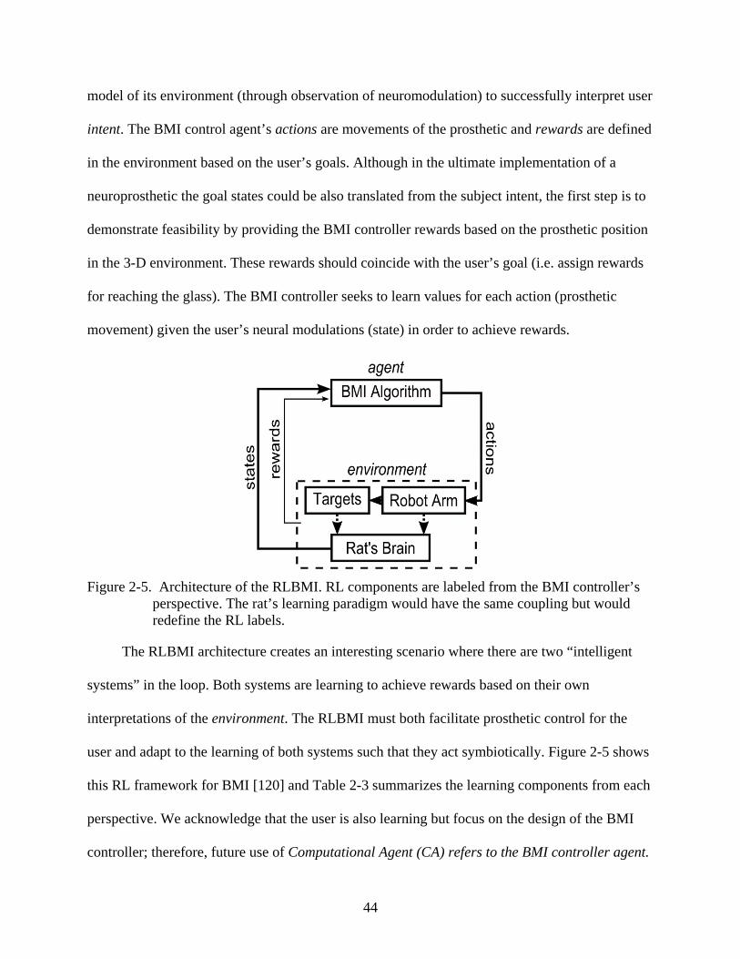
44

model of its environment (through observation of neuromodulation) to successfully interpret user

intent. The BMI control agent’s actions are movements of the prosthetic and rewards are defined

in the environment based on the user’s goals. Although in the ultimate implementation of a

neuroprosthetic the goal states could be also translated from the subject intent, the first step is to

demonstrate feasibility by providing the BMI controller rewards based on the prosthetic position

in the 3-D environment. These rewards should coincide with the user’s goal (i.e. assign rewards

for reaching the glass). The BMI controller seeks to learn values for each action (prosthetic

movement) given the user’s neural modulations (state) in order to achieve rewards.

Figure 2-5. Architecture of the RLBMI. RL components are labeled from the BMI controller’s

perspective. The rat’s learning paradigm would have the same coupling but would redefine the RL labels.

The RLBMI architecture creates an interesting scenario where there are two “intelligent

systems” in the loop. Both systems are learning to achieve rewards based on their own

interpretations of the environment. The RLBMI must both facilitate prosthetic control for the

user and adapt to the learning of both systems such that they act symbiotically. Figure 2-5 shows

this RL framework for BMI [120] and Table 2-3 summarizes the learning components from each

perspective. We acknowledge that the user is also learning but focus on the design of the BMI

controller; therefore, future use of Computational Agent (CA) refers to the BMI controller agent.

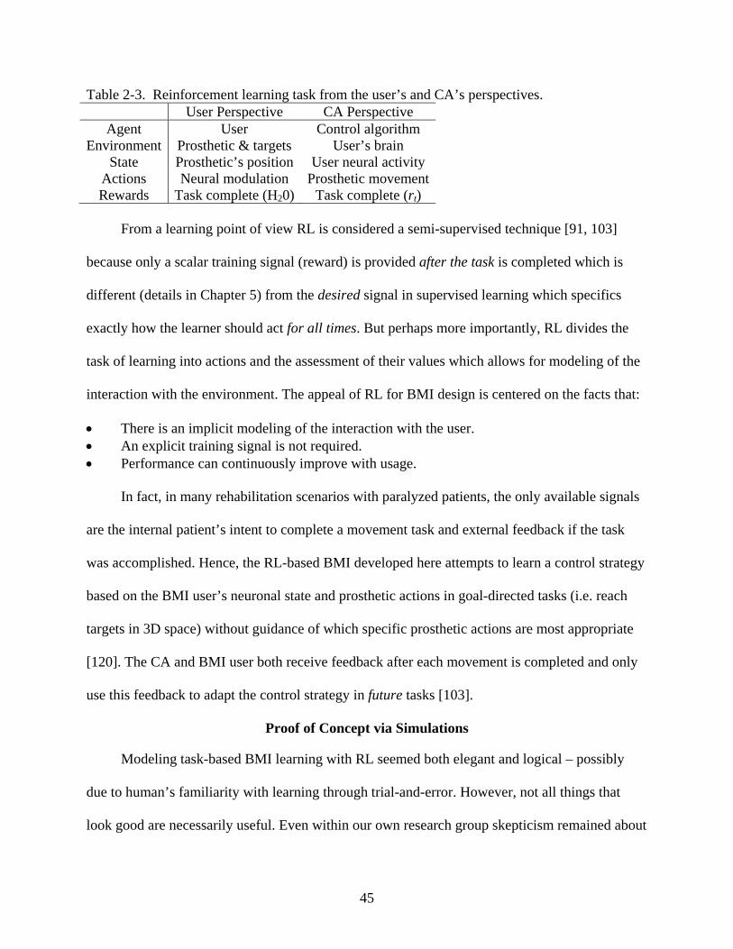
45

Table 2-3. Reinforcement learning task from the user’s and CA’s perspectives. User Perspective CA Perspective

Agent User Control algorithm Environment Prosthetic & targets User’s brain

State Prosthetic’s position User neural activity Actions Neural modulation Prosthetic movement Rewards Task complete (H20) Task complete (rt)

From a learning point of view RL is considered a semi-supervised technique [91, 103]

because only a scalar training signal (reward) is provided after the task is completed which is

different (details in Chapter 5) from the desired signal in supervised learning which specifics

exactly how the learner should act for all times. But perhaps more importantly, RL divides the

task of learning into actions and the assessment of their values which allows for modeling of the

interaction with the environment. The appeal of RL for BMI design is centered on the facts that:

• There is an implicit modeling of the interaction with the user. • An explicit training signal is not required. • Performance can continuously improve with usage.

In fact, in many rehabilitation scenarios with paralyzed patients, the only available signals

are the internal patient’s intent to complete a movement task and external feedback if the task

was accomplished. Hence, the RL-based BMI developed here attempts to learn a control strategy

based on the BMI user’s neuronal state and prosthetic actions in goal-directed tasks (i.e. reach

targets in 3D space) without guidance of which specific prosthetic actions are most appropriate

[120]. The CA and BMI user both receive feedback after each movement is completed and only

use this feedback to adapt the control strategy in future tasks [103].

Proof of Concept via Simulations

Modeling task-based BMI learning with RL seemed both elegant and logical – possibly

due to human’s familiarity with learning through trial-and-error. However, not all things that

look good are necessarily useful. Even within our own research group skepticism remained about

46

this RL modeling of the BMI task with two intelligent systems. Before investing time and

resources to develop a closed-loop BMI paradigm, we first decided to address a series of issues

that would be crucial to the future success of this architecture.

• Do the rat’s neural modulations form states which the CA can exploit? • What RLBMI control complexity (e.g. 1, 2, or 3 dimensions) is feasible? • Can we ensure that the CA is using information in the neural modulations only? • Which set of RL parameters facilitates BMI control; is control robust over parameters? • What challenges are likely to arise in closed-loop implementation?

These questions were addressed in a conference publication [120] using off-line

multielectrode recordings from a behaving rat [104]. This answered the skeptics and motivated

further RLBMI development. A brief summary of the findings for each issue will be presented

in the next subsections. Explicit details of the behavioral paradigm and BMI architecture/

training will be given in chapters 3 & 5 respectively for the closed-loop paradigm. The

simulations used a similar, but less complex paradigm and BMI architecture and training. Future

chapters provide more details but these summaries should be sufficient to prove the concept.

Do the rat’s neural modulations form states which the CA can exploit?

Prior literature has clearly shown control tasks can be robustly modeled with RL and if the

state is repeatable with respect to the actions that should be taken [103]. However, in this

literature, any lack of repeatability in the state is likely due to sensor noise and the state-actions

pairs still have a deterministic relationship with future states. This RLBMI architecture de-

couples the relationship between current and future states and works in a much higher

dimensional state space. Knowing that repeatable states were a prerequisite for control, we

attempted to find repeatability in a state based on neural data (see Figure 2-5).

Estimated neural FR from the forelimb regions of each hemisphere were recorded from a

rat during a two-lever choice behavioral task as described in [104]. The task was modified such

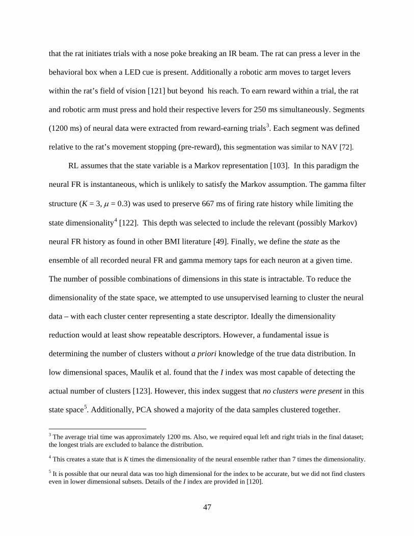
47

that the rat initiates trials with a nose poke breaking an IR beam. The rat can press a lever in the

behavioral box when a LED cue is present. Additionally a robotic arm moves to target levers

within the rat’s field of vision [121] but beyond his reach. To earn reward within a trial, the rat

and robotic arm must press and hold their respective levers for 250 ms simultaneously. Segments

(1200 ms) of neural data were extracted from reward-earning trials3. Each segment was defined

relative to the rat’s movement stopping (pre-reward), this segmentation was similar to NAV [72].

RL assumes that the state variable is a Markov representation [103]. In this paradigm the

neural FR is instantaneous, which is unlikely to satisfy the Markov assumption. The gamma filter

structure (K = 3, µ = 0.3) was used to preserve 667 ms of firing rate history while limiting the

state dimensionality4 [122]. This depth was selected to include the relevant (possibly Markov)

neural FR history as found in other BMI literature [49]. Finally, we define the state as the

ensemble of all recorded neural FR and gamma memory taps for each neuron at a given time.

The number of possible combinations of dimensions in this state is intractable. To reduce the

dimensionality of the state space, we attempted to use unsupervised learning to cluster the neural

data – with each cluster center representing a state descriptor. Ideally the dimensionality

reduction would at least show repeatable descriptors. However, a fundamental issue is

determining the number of clusters without a priori knowledge of the true data distribution. In

low dimensional spaces, Maulik et al. found that the I index was most capable of detecting the

actual number of clusters [123]. However, this index suggest that no clusters were present in this

state space5. Additionally, PCA showed a majority of the data samples clustered together.

3 The average trial time was approximately 1200 ms. Also, we required equal left and right trials in the final dataset; the longest trials are excluded to balance the distribution.

4 This creates a state that is K times the dimensionality of the neural ensemble rather than 7 times the dimensionality.

5 It is possible that our neural data was too high dimensional for the index to be accurate, but we did not find clusters even in lower dimensional subsets. Details of the I index are provided in [120].

48

Due to the above limitations in the clustering approach, we decided to use more of the

temporal-spatial relationships in the neural signal to define the state. We use artificial multi layer

perceptrons (MLP) with three hyperbolic tangent nonlinearities to segment the state (input to the

MLP) and one linear output processing elements (PE) for each action to estimate the value for

that action given the state. Hence, the MLP is a Value Function Estimation (VFE) network, The

MLP are trained on-line using Q(λ) learning, which is an off-policy RL method that learns from

sequences of state-action pairs [103]. This algorithm is a proven technique that is appropriate for

lower dimensional ‘noisy’ states [103]. An ε-greedy policy was used because the soft-max policy

was unstable for this application. There are 46 trials (12 states per trial) to train the neural

networks and 16 trials are reserved for testing.

After training the networks, the RLBMI could achieve goal directed movements of

prosthetic limbs over 80% of the time (see Table 2-4). This performance was calculated on the

novel test-set of neural states. While we could not visualize repeatability in the high dimensional

state, if the state was segmented through a MLP there was some repeatable state feature that

could be used for action selection to solve two different tasks. This performance provided

confidence that the ensemble of neural FR and histories could be used as the RLBMI state. The

next, related question is what control complexity can be achieved with these states.

What RLBMI control complexity (e.g. 1, 2, or 3 dimensions) is feasible?

To determine the complexity of possible RLBMI control, we simulated robot control in

one, two, and three dimensions. In any case, there are two targets equidistant from the robot’s

starting position. Depending on the dimension of the control space, there are up to 26 possible

actions: moving 1 unit in any single direction, moving 0.7 units6 in any direction pairs, and

6 The different scales for multi-dimension moves restrict all action vectors to the same length.

49

moving 0.6 units in any direction triples. If the robot reaches a target within 10 steps (10

consecutive neural states), a positive reward is generated, the trial ends, and the robot is reset to

the initial position. Otherwise the trial is failed and ends. To benchmark performance, the

probabilities of randomly7 reaching the target for the two and three dimension tasks are 4.7e-7

and 8.4e-8 respectively. Further surrogate tests will be provided in the next subsection.

We use the Percentage of trials earning Rewards (PR) to quantify performance in this task-

based control. Table 2-4 shows that performance is above 80% in the test set for all dimensions

tested. These results provided confidence that the RLBMI would be useful to control a robot in

three dimensions. However, it does not prove that the CA used information in the neural state.

Table 2-4. RLBMI test set performance (PR) for different workspace dimensionality Dimension Maximum Mean Standard Deviation

1 92.3 % 92.3 % n/a 2 81.3 % 61.9 % 10 % 3 81.3 % 68.1 % 10.8%

Results are the average of 10 trained networks, except 1D data which was only processed once Can we ensure that the CA is using information in the neural modulations only?

The robot position was not included in the state because that information would reduce the

learning problem to a basic ‘grid-world’ [103] where neural components of the state vector

would be ignored. However, since this RLBMI is a new architecture it was important to satisfy

concerns that the system could be tracking (a phenomenon that affects SL when it follows only

the prior desired signal) or learning from some other unspecified and unobservable state. To

counter these preconceptions, we created a surrogate data set. The spatial and temporal

relationships in the neural data were randomized to create a surrogate data set; this set was used

to test the null hypothesis that the RLBMI could learn independently of the neural state.

7 The benchmark probability is calculated by approximating the action selection as a Bernoulli random variable.

50

RLBMI trained with neural data had at least 30% better performance than RLBMI trained

with surrogate data. Table 2-5 compares neural vs. surrogate performance for 2D and 3D control.

This result provided confidence that there is information in the neural state and the RLBMI could

successfully extract this information. It also shows PR is affected by parameter selection

(RLBMI using exploration are marked with *). The next section addresses the robustness of

RLBMI control.

Table 2-5. Test set performance (PR) using states consisting of neural vs. surrogate data States Dimension Maximum Mean Standard Deviation

Neural 2 81.3 % 61.9 % 10 % Neural 3 81.3 % 68.1 % 10.8% Neural 3* 75 % 50 % 15.6 %

Surrogate 2 43.8 % 23.1 % 11 % Surrogate 3 43.8 % 34.3 % 7.3 % Surrogate 3* 43.8 % 31.8 % 8.56 % ∗ ∼5% of trials were exploratory (ε = 0.005). λ = 0.8 with 3 hidden PEs for 3D tests. λ = 0.8571 with 2 hidden PEs for 2D tests

The surrogate data was able to control the robot at levels higher than predicted by the

random walk model in the prior section. This increase in performance is logical because the CA

learns to change the randomness in the walk despite the lack of information in the surrogate data.

When training with surrogate data, the RLBMI can randomly reach a target. The CA then

reinforces the action to reach that target. Effectively the CA guesses a target direction which

changes the chance performance in a two-target task to 50% (100% for one target and 0% for the

other target). RLBMI with surrogate data still outperforming the random walks is a recurring

problem that will be revisited in Chapter 5.

Finding a RL parameter set for robust control

The final issue is whether we could find a set of RL parameters which would both facilitate

stable control but also be robust to small changes in the parameters. We searched the RLBMI

parameter space based on related literature and observations of learning performance. If

51

α, Η, and λ were selected appropriately, the RLBMI converges. α are the learning rates for the

MLP, H is the number of hidden layer PEs in the MLP and λ is a term which weights inclusion

future estimates of return. (Full details of the all system parameters are given in chapter 5.)

Training set performance was robust to parameter selection as expected; however, test set

generalization was only possible with certain parameter combinations. We were able to simplify

the search, because the task is episodic it was logical to set γ to one. A range of λ centered

around (1-1/(trial length)) were tested to find the test set generalization. H was selected based on

the principal components of the trajectory as has been shown in other BMI literature [124].

Figure 2-6 shows the average and best performance PR over a range of possible λ in two

different sets of MLP learning rates which differ by 5x. Obviously we cannot claim to have

exhausted all of the possible RL BMI parameter set combinations; however, Figure 2-6 shows

that PR is fairly robust over a range of α and λ. We have found parameter sets that illustrate the

potential of RL BMI, even if they are not optimal parameters.

40

60

80

0.680.70.720.740.760.780.80.820.840.86

40

60

80

Lambda

% o

f Tria

ls E

arni

ng R

ewar

d (P

R)

alphaIL = 0.01, alphaHL 0.001

alphaIL = 0.05, alphaHL 0.005

Figure 2-6. RLBMI performance over a range of α and λ. The average (solid) and best (dashed)

performance of 10 runs is presented for two different α sets.

52

What challenges are likely to arise in closed-loop implementation?

Table 2-4 illustrated that the RLBMI could achieve goal directed movements of prosthetic

limbs in three dimensions over 80% of the time. Furthermore we disproved the null hypothesis

that RL could solve tasks using information from the model of the robot environment or some

other unknown information source. While RLBMI could learn (memorize) the surrogate training

data, it does not generalize to novel data. These results support our assertion that there is

movement-related information present in the neural data which RLBMI can exploit. Finally, we

showed that the RLBMI was robust over a limited range of parameter selection.

However, there are research challenges which may arise in the closed-loop RLBMI and

could not be simulated in the offline analysis. It is not possible to generate biofeedback in these

experiments such that the rat could adjust his neural modulations. We anticipate that biofeedback

will encourage the rat to modulate neural activity (create states) based on the rat’s view of the

environment. This strengthening of the state-action relationship should improve control.

The second problem is the data segmentation used to extract specific sequences of states.

While it increased the likelihood of extracting behaviorally related modulations, it is infeasible in

closed-loop experiments. It is not a causal technique and moreover there would be no rat

movements in closed loop control as landmarks for segmentation. Future experiments can not

use segmentation based on movement cues.

There is randomness inherent in both Q(λ) action selection and the initialization of MLP

weights; this creates another potential issue where the RLBMI performance is partially a

function of both initialization and action selection. Multiple networks will be trained in closed

loop control in order to find the highest performance (PR) and overcome this issue. A related

issue is learning speed, the offline experiments required up to 250 epochs of training [120] in

53

order to generalize to novel neural data. It is necessary to devise a way to provide the necessary

computational power to achieve this training in closed loop control.

Possible Implications of this Paradigm

This new paradigm creates a situation where there are two tightly coupled learning

systems: the rat and the CA. These learners should co-adapt to achieve control of the robot.

While the rat is learning which neuronal modulations result in water rewards, the CA must adapt

to more effectively respond to the rat’s brain to earn external rewards8. Obviously this creates a

principled method for learning BMI control without a desired signal. This not only avoids the

necessity of patient movements, but also creates the possibility of constant co-adaptation even in

brain-control. Additionally, since both learners have a shared reward and both use the same

learning mechanism, this co-adaptation may be synergistic and allow increased control

complexity or speed of acquiring control. A feature notably absent from the RLBMI so far was

restrictions on the neural signals of robot actions used. This architecture not only shifted the

paradigm, but also seemed viable for many different BMI control applications.

Alternative RLBMI States

The state must to be representative of the environment and relatively (more is better)

repeatable with respect to selecting actions. Even in our simulations we show that the state can

be preprocessed and transformed to meet this requirement. We used binned estimates of MI

single unit activity because that is known to relate to the rat actions (which is the CA’s

environment). BCI research in a rabbit model at Advanced Robotics Technologies & Systems

Lab (Scuola Superiore Sant’Anna), revealed electroneurographic (ENG) signals could be

extracted from the gastrocnemius nerve in a rabbit [125]. This ENG signal was repeatable with

8 Rewards for the CA and their relationship to the rat’s rewards are described in Chapter 3 and Appendix A.

54

respect to ankle flexion. Furthermore, the signal required minimal preprocessing of wavelet de-

noising and uni-directional thresholding as opposed to traditional power and time-intensive spike

sorting. This type of state could be ideally coupled with the low power (see Chapter 4) RLBMI

while respecting the computational power limitations of an implantable prosthetic controller.

More details of my research in the ARTS lab are provided in Appendix D.

Alternative RLBMI Actions

In the offline simulations, we assigned a Cartesian action set to give the RLBMI maximal

control degrees of freedom. However, we could have easily given an order of magnitude more or

less action in the set. While the dimensionality of the action set will affect Q learning speed

[103], the RLBMI should still co-adapt to a solution. The actions only are required to affect the

environment to be useful. Theoretically actions could include the movemes from earlier work

[108]. It was two years after proposing the RLBMI that was able I revisited the topic of

movemes at Daniel Wolpert’s Sensory Motor Control Group at Cambridge University. There I

was not constrained by species mismatches and experimental constraints. Instead, I investigated

hours of unconstrained hand movements to find any natural primitives or correlations.

Wolpert and Kawato originally designed the MPFIM of motor control in 1998 which used

motion primitives (these primitives naturally parallel RLBMI actions) [16]. However, he has

moved away from this idea of movemes because there is no evidence of human subjects actually

being able to switch between multiple motor control models and motion segmentation is much

too subjective. Undeterred, I investigated the neuroethology of hand movement and was able to

find correlations in the principle components of hand control for different human subjects. This

multiple models principle, whether biologically meaningful or not, remains a viable engineering

solution with potential to improve prosthetic control. This principle could easily be incorporated

into the RLBMI. More details of my research in Dr. Wolpert’s lab are provided in Appendix C.

55

CHAPTER 3 CHANGING THE BEHAVIORAL PARADIGM

Learning the Importance of a Behavioral Paradigm

Animal training is fundamentally different than algorithm design; therefore it merits a

separate chapter. However, there was significant chronological overlap between the RLBMI

development in Chapter 2 and development of the rat model for BMI. In fact, some of the

insights gained from the rats were critical for designing the architecture. Once again, the

contributions would evolve from an established supervised learning foundation.

Initial Rat BMI Model

In 2004 Sanchez developed a rat BMI model to facilitate rapid testing of both BMI

algorithms and hardware developed at the University of Florida [109, 126-128]. The paradigm

was modeled from a standard two-lever choice task [119] and it provided access to the rat’s

neuronal modulations, the LED cues, and lever positions (pressed vs. not pressed) which were all

recorded on a shared time clock1. It was reasonable to use the quasi-binary lever positions as

desired signals because the rat’s movements are ballistic [121, 129], i.e. all of the information in

the motion should be contained in the start and end points.

The operating environment is shown in Figure 3-1 from a rat’s eye view. The rat’s task

was relatively straightforward – both levers were periodically extended and an LED would cue

the rat which side to press. The rat received a 0.04 mL water reward (and heard a 1 kHz tone) if

he pressed the cued lever with 23.5 g/cm2 force and held it for 500 ms [109]. The rat was not

explicitly penalized for pressing the un-cued lever, but also was not rewarded. The amount of

time the levers were retracted and extended was preset by the experimenter and the cued side

was randomly selected while the experiment was running. The lever extension-retraction cycle

1 The neural modulations are sampled at 244141.1 Hz and the other signals are sampled at 384.1 Hz.

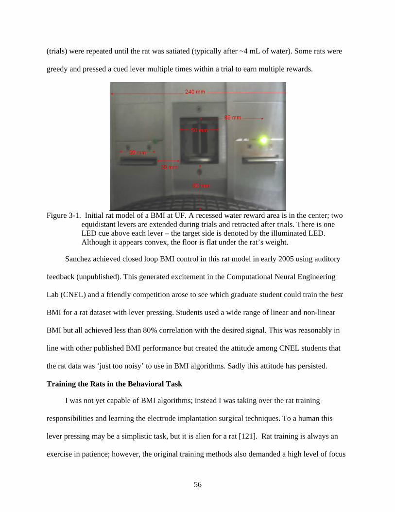
56

(trials) were repeated until the rat was satiated (typically after ~4 mL of water). Some rats were

greedy and pressed a cued lever multiple times within a trial to earn multiple rewards.

Figure 3-1. Initial rat model of a BMI at UF. A recessed water reward area is in the center; two

equidistant levers are extended during trials and retracted after trials. There is one LED cue above each lever – the target side is denoted by the illuminated LED. Although it appears convex, the floor is flat under the rat’s weight.

Sanchez achieved closed loop BMI control in this rat model in early 2005 using auditory

feedback (unpublished). This generated excitement in the Computational Neural Engineering

Lab (CNEL) and a friendly competition arose to see which graduate student could train the best

BMI for a rat dataset with lever pressing. Students used a wide range of linear and non-linear

BMI but all achieved less than 80% correlation with the desired signal. This was reasonably in

line with other published BMI performance but created the attitude among CNEL students that

the rat data was ‘just too noisy’ to use in BMI algorithms. Sadly this attitude has persisted.

Training the Rats in the Behavioral Task

I was not yet capable of BMI algorithms; instead I was taking over the rat training

responsibilities and learning the electrode implantation surgical techniques. To a human this

lever pressing may be a simplistic task, but it is alien for a rat [121]. Rat training is always an

exercise in patience; however, the original training methods also demanded a high level of focus

57

and precise reaction times from the trainer especially when the rat was first learning the

associations. The challenge arose because the rat was not learning what the trainer envisioned –

considering the cues, making the correct decision, stereotypically pressing the lever, and then

going to the reward center after hearing the tone. The rat behavior suggested interest only in

maximizing rewards. For example, rats were prone to immediately press one lever at trial start

(seemingly oblivious to the cues) and if no reward was observed, then press the other lever. This

type of behavior was not cue-related and the corrective behavior was less likely to be

stereotypical; hence more difficult for a BMI to reproduce. This created a battle of wills with the

trainer only able to turn off cues, adjust the press threshold to make earning rewards more

difficult, or manually reward the rat (see Figure 3-2) by pressing buttons within a trial. If the

trainer was not fast enough or made a mistake, the rat was rewarded for bad behavior.

Figure 3-2. Initial controls for training rats in the BMI paradigm. A digital plot of the lever

positions was also available but is not shown.

Sanchez had previously trained the rats and I was beginning to slowly succeed also.

However, after much frustration and multiple unsuccessful conversations with the rats, I

critically evaluated this training and decided I needed four things:

• More clear task definition for the rat. • More precise control of all paradigm aspects. • Maintaining the ability to automate advanced training. • Enforce the stereotypical behavior assumption.

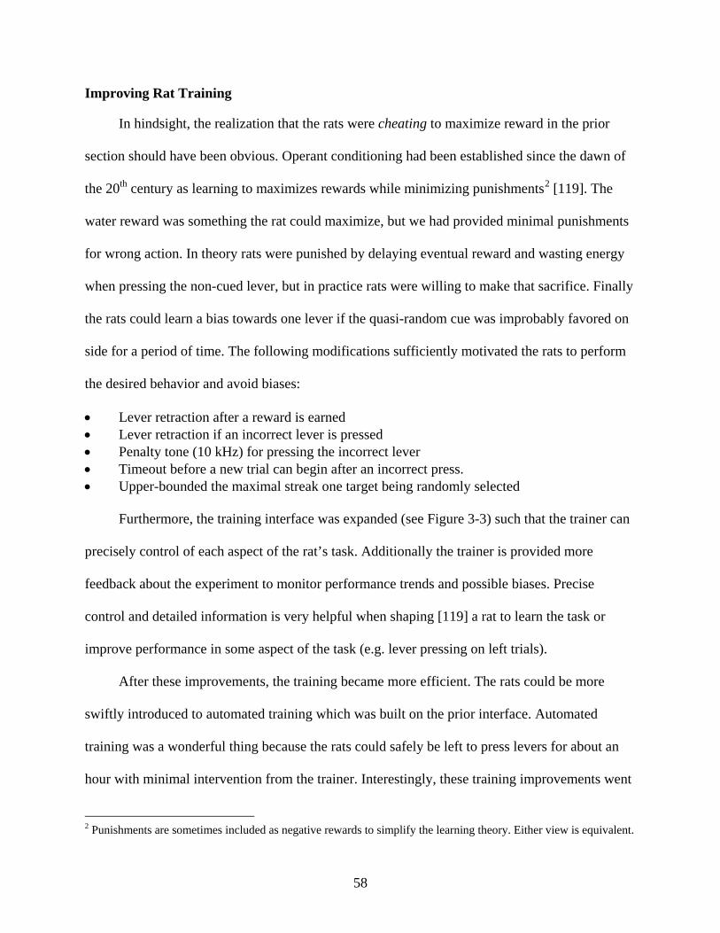
58

Improving Rat Training

In hindsight, the realization that the rats were cheating to maximize reward in the prior

section should have been obvious. Operant conditioning had been established since the dawn of

the 20th century as learning to maximizes rewards while minimizing punishments2 [119]. The

water reward was something the rat could maximize, but we had provided minimal punishments

for wrong action. In theory rats were punished by delaying eventual reward and wasting energy

when pressing the non-cued lever, but in practice rats were willing to make that sacrifice. Finally

the rats could learn a bias towards one lever if the quasi-random cue was improbably favored on

side for a period of time. The following modifications sufficiently motivated the rats to perform

the desired behavior and avoid biases:

• Lever retraction after a reward is earned • Lever retraction if an incorrect lever is pressed • Penalty tone (10 kHz) for pressing the incorrect lever • Timeout before a new trial can begin after an incorrect press. • Upper-bounded the maximal streak one target being randomly selected

Furthermore, the training interface was expanded (see Figure 3-3) such that the trainer can

precisely control of each aspect of the rat’s task. Additionally the trainer is provided more

feedback about the experiment to monitor performance trends and possible biases. Precise

control and detailed information is very helpful when shaping [119] a rat to learn the task or

improve performance in some aspect of the task (e.g. lever pressing on left trials).

After these improvements, the training became more efficient. The rats could be more

swiftly introduced to automated training which was built on the prior interface. Automated

training was a wonderful thing because the rats could safely be left to press levers for about an

hour with minimal intervention from the trainer. Interestingly, these training improvements went

2 Punishments are sometimes included as negative rewards to simplify the learning theory. Either view is equivalent.

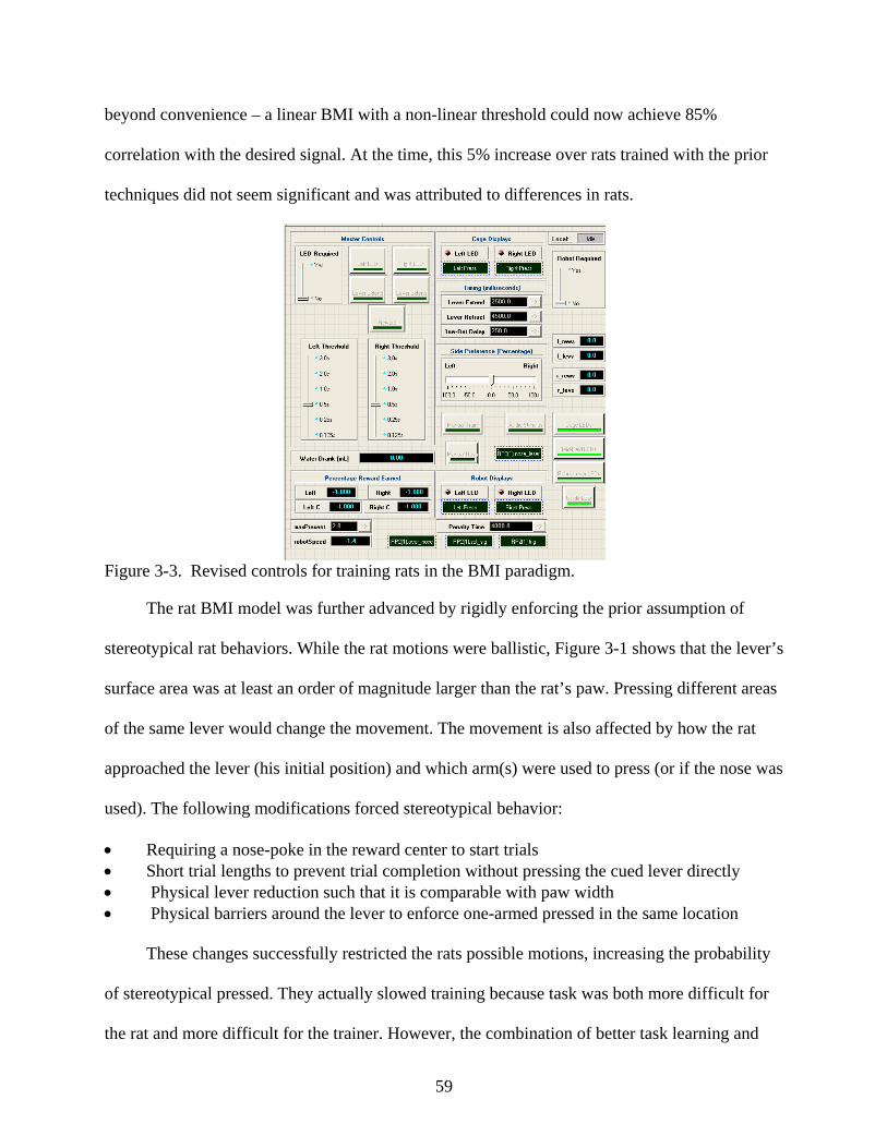
59

beyond convenience – a linear BMI with a non-linear threshold could now achieve 85%

correlation with the desired signal. At the time, this 5% increase over rats trained with the prior

techniques did not seem significant and was attributed to differences in rats.

Figure 3-3. Revised controls for training rats in the BMI paradigm.

The rat BMI model was further advanced by rigidly enforcing the prior assumption of

stereotypical rat behaviors. While the rat motions were ballistic, Figure 3-1 shows that the lever’s

surface area was at least an order of magnitude larger than the rat’s paw. Pressing different areas

of the same lever would change the movement. The movement is also affected by how the rat

approached the lever (his initial position) and which arm(s) were used to press (or if the nose was

used). The following modifications forced stereotypical behavior:

• Requiring a nose-poke in the reward center to start trials • Short trial lengths to prevent trial completion without pressing the cued lever directly • Physical lever reduction such that it is comparable with paw width • Physical barriers around the lever to enforce one-armed pressed in the same location

These changes successfully restricted the rats possible motions, increasing the probability

of stereotypical pressed. They actually slowed training because task was both more difficult for

the rat and more difficult for the trainer. However, the combination of better task learning and

60

more stereotypical reaching behavior further improved linear BMI reconstruction. Now the

output was more than 91% correlated with the desired signals.

Lessons Learned

Although my initial motivation was to make the training process easier on myself, the end

result was that the rats became a superior BMI model. This was an early lesson in the critical

importance in personal involvement in quality paradigm design before addressing a research

question. This lesson was reaffirmed years later when I had the privilege to work with some of

the worlds leading experts in human motor control theory at the Sensory Motor Control Group.

There they typically did not have access to any physiological signals at a lower level of

abstraction than electromyographic (EMG) activations. Instead they typically focused on simple

descriptors like endpoint position, timing, or arm configuration. Through careful experimental

design with appropriate constraints, these descriptors were sufficient to advance understanding of

the motor control system. Without good design, results were much less valuable.

By this point I was training up to four rats every day. Even with the training improvements

the sheer amount of time involved was too much for one person. Fortunately my friend and

colleague Babak had joined the lab and took on half of the training responsibility. In a similar bid

to save himself time, he switched to the automated training much earlier in the training process

than I normally would for his rats. Surprisingly, his rats began to outperform my rats – learning

faster and achieving higher success (% of trials earning reward). We realized that the unbiased

precision of the computer training was superior to any assistance I thought only a human could

provide. This immediately reduced overall rat training time by 2 weeks.

Carefully designed rewards and penalties allowed the use of operant conditioning (RL) to

train the rats to achieve a complex and alien task. Physical constraints in the environment also

could control rat behavior to support an initially strong experimental assumption. Finally, the

61

repeatable relationships between paradigm states, rat actions, and rewards helped the rats learn

faster and perform better. All these concepts began strongly influence the RLBMI architecture

that I was proposing around the same time. The experimental paradigm for the rat RLBMI model

was meticulously developed to incorporate these concepts and lessons learned.

Designing the Rat’s Environment

Male Sprague-Dawley rats were trained3 in a two-lever choice task via operant

conditioning to associate robot control with lever pressing [119]. The experimental paradigm

will be used to support the operant conditioning of the rat and closed-loop brain control of a

robot arm using RLBMI. Naturally this paradigm is a departure from prior SL BMI paradigms

which operated with different assumptions and goals. We designed a two-target choice task in a

rat model of a paralyzed patient that is seeking to control a prosthetic. The rat must maneuver a

five DOF robotic arm (Dynaservo, Markham ON) based on visual feedback to reach a set of

targets and earn a water reward. The paradigm fits the RLBMI framework because both the rat

and CA can earn rewards through interaction with their environments. Both intelligent systems

are initially naïve in the closed-loop control task and must co-adapt over multiple4 trials to learn

the tasks over multiple days (sessions) of training.

As shown in Figure 3-4, the rat is enclosed in a behavioral cage with plexiglass walls.

There are two sets of retractable levers (Med Associates, St. Albans VT): the set within the

behavioral cage is referred to as cage levers; the set in the robotic workspace is referred to as

target levers. A solenoid controller (Med Associates) dispenses 0.04 mL of water into the reward

center on successful trials. An IR beam (Med Associates) passes through the most distal portion

3 Rats were motivated using a 21 hour water withholding protocol approved by the University of Florida IACUC.

4 The number of trials depended on rat motivation and performance in each session; the range of trials per session was 86-236.

62

of the reward center. There are three sets of green LEDs: the set immediately behind the cage

levers are cage LEDs, the set in the robot workspace are midfield LEDs, and the set on the target

levers are target LEDs. The positioning of the three sets of LEDs and levers offers a technique to

guide attention from inside the cage to the robot environment outside. There is one additional

blue LED mounted to the robot endpoint; it is referred to as the guide LED and it is used to assist

the rat in tracking the position of the robot. Because the behavioral cage walls are constructed

from plexiglass, the robotic workspace is within the rat’s field of vision [121].

The rat operates in low-light conditions to activate the more sensitive rods in the rat visual

system [121]. The LED cues in this system emit green (~510 nm) light and the LED guide light

attached to the robot emits blue (~475 nm) light. Rat’s retinas contain only 1% cones; however,

the peak sensitivity for the majority of these cones is at 510 nm [121]. Rat’s visual acuity is also

lower than humans (especially albino rats as were used in this study); however, we designed the

robot workspace and targets to maximize the angle subtended by the robotic targets to the rat’s

eye. Additionally, we used target and guide LED to maximize contrast for the rat.

Figure 3-4. Workspace for the animal model. Detailed landmarks are provided in Appendix A.

63

Animal Training through Behaviorist Concepts

Initially, the robotic arm tip (guide LED) is positioned directly in front of the water reward

center. The rat initiates a trial (see Figure 3-5) with a nose-poke through the IR beam in the

reward center. The target side and robot speed are randomly selected. All levers are extended

synchronously and LEDs on the target side are illuminated to cue the rat. The robot follows a

pre-determined trajectory to reach the target lever within 0.8-1.8 s and the robot will only press

the target levers while the rat is pressing the correct cage lever. If the correct cage and target

levers are pressed concurrently for 500 ms then the task is successfully completed; a water

reward positively reinforces the rat’s association of the robot lever pressing with reward and the

trial is ended. If the rat presses the incorrect cage lever at any time, the trial is aborted, a brief

tone indicates the choice was wrong, and there is a timeout (4-8 s) before the next trial can begin.

Additionally, if the task is not completed within 2.5 s the trial is ended. Whenever a trial ends: all

levers are retracted, the LEDs are turned off, and the robot is reset to the initial position. A 4 s

refractory period prevents a new trial while the rat may be drinking.

Figure 3-5. Rat training timeline.

Training a rat to complete this multi-part task involving synergistic activity with a robot

(roughly 10x larger than the rat) using primarily visual feedback from an external workspace is a

non-trivial challenge. However, through the operant conditioning techniques of chaining and

shaping the rats learn to achieve this difficult task [119]. Initially, the first necessary behavior

(i.e. nose-poke to break the IR beam) is positively reinforced (water reward). This reinforcement

conditions the rat to perform the nose-poke behavior. After the rat becomes proficient at the

64

initial behavior, that behavior (i.e. nose-poke) is no longer positively reinforced. Instead the rat

must complete the initial behavior and then a subsequent behavior (i.e. move towards the target

lever). The subsequent behavior is then positively reinforced. This chaining continues throughout

all behavioral segments of the paradigm until the rat finally is capable of completing the entire

task and only the final behavior is positively reinforced. Variable time constraints are used to

shape each segment of the chain – initially the animal is rewarded for completing the task (e.g.

press levers for 125 ms) within 6 s, but through shaping the rat becomes able to complete the

task (e.g. press levers for 500 ms) within 2.5 s.

The rat initially seems aware only of the cage levers, and learns to press the correct lever to

produce the water reward when all LEDs for a given side light up. The rat is then further shaped

to attend to the robot workspace by gradually moving the center of attention from within the cage

to the robot workspace outside. This is achieved through turning off cage and midfield LED cues

(see Figure 3-1) in sequence during training. The variable robot speed also encourages attention

to the robot - the rat can minimize task energy by synchronizing pressing with the robot.

Eventually, the rat cues are reduced to the proximity of the guide LED to the target LED for

completing the task and obtaining water. The rats learn to perform stereotypical motions for the

environmental cues [121]. Barriers restrict access to cage levers such that rat only presses with

the contra-lateral arm in a stereotypical fashion. The timeout and time-limit both encourage

correct behavior - rats can maximize water rewards earned by avoiding timeouts and

unsuccessful trials. These measures to enforce attention to the robot workspace and stereotypical

behavior are crucial to the rat RLBMI model - they couple the relative positions of the robot and

targets to the rat’s neuronal modulations. This coupling respects the assumptions proposed in the

state definition of the CA.

65

The percentage of trials earning a reward is used to judge the rat’s ability to discriminate

between targets using visual cues and complete the task. The rat’s accuracy must exceed an

inclusion criterion of 80%. Rats incapable of this inclusion criterion within 25 days were

excluded. The inclusion criteria was designed such that the experiment only uses rats which are

actively deciding between targets based on visual cues and successfully completing the task. The

criteria also considered prior rat accuracy in this and similar paradigms [120] – rat performance

typically plateaus above 80%.

Microelectrode Array Implantation

Rats that reach the operant conditioning inclusion criterion were chronically implanted

bilaterally with two microelectrode arrays in layer V of the caudal forelimb area in the primary

motor cortex (MI) [29, 130]. Neuronal signals are recorded from the caudal forelimb area of MI

because this area has been shown to be predictive of limb motion in a rat; additionally, similar

modulations occur when operating a BMI without physical movements [56]. The rats are not

implanted before reaching the inclusion criteria to avoid two potential issues. The known cortical

motor map reorganization during skilled task learning [28-30] could distort the state signal. Also,

the immune response and electrode structural degradation limit recording time [127].

The rats were anesthetized with inhaled isoflourane (1.5% in O2 flowing at 0.6 L/min) and

also injected with Xylazine (10mg/kg dose) to maintain a stable anesthesia plane. The rat’s vital

signs are closely monitored by the surgeon throughout the entire procedure to ensure stability of

the anesthesia plane and the rat’s general health. A heating pad is used preserve the rat’s body

temperature and eye lube is applied for protection over the long procedure.

The rat’s head is shaved; then the surgical site is sterilized to prevent infection. A midline

incision is made, and the periosteum is scraped away to expose the skull between the temporal

ridges. Bilateral craniotomies are drilled 1.0 mm anterior and 2.5 mm lateral to bregma using a

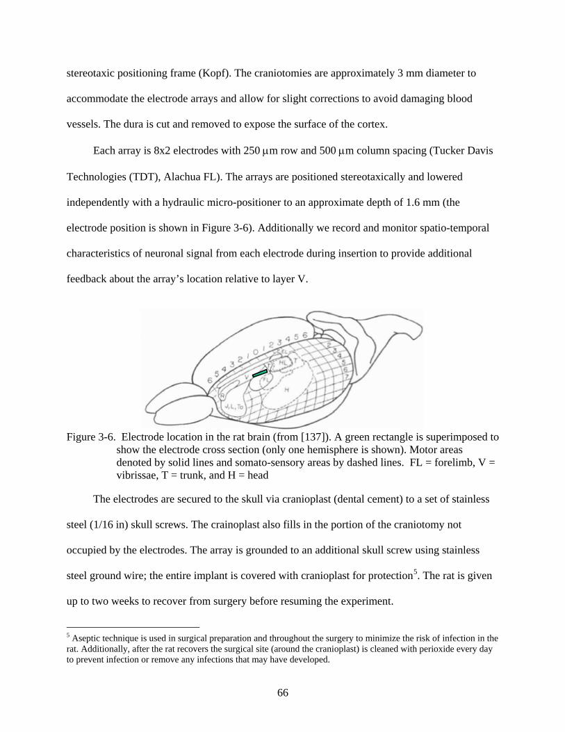
66

stereotaxic positioning frame (Kopf). The craniotomies are approximately 3 mm diameter to

accommodate the electrode arrays and allow for slight corrections to avoid damaging blood

vessels. The dura is cut and removed to expose the surface of the cortex.

Each array is 8x2 electrodes with 250 µm row and 500 µm column spacing (Tucker Davis

Technologies (TDT), Alachua FL). The arrays are positioned stereotaxically and lowered

independently with a hydraulic micro-positioner to an approximate depth of 1.6 mm (the

electrode position is shown in Figure 3-6). Additionally we record and monitor spatio-temporal

characteristics of neuronal signal from each electrode during insertion to provide additional

feedback about the array’s location relative to layer V.

Figure 3-6. Electrode location in the rat brain (from [137]). A green rectangle is superimposed to

show the electrode cross section (only one hemisphere is shown). Motor areas denoted by solid lines and somato-sensory areas by dashed lines. FL = forelimb, V = vibrissae, T = trunk, and H = head

The electrodes are secured to the skull via cranioplast (dental cement) to a set of stainless

steel (1/16 in) skull screws. The crainoplast also fills in the portion of the craniotomy not

occupied by the electrodes. The array is grounded to an additional skull screw using stainless

steel ground wire; the entire implant is covered with cranioplast for protection5. The rat is given

up to two weeks to recover from surgery before resuming the experiment.

5 Aseptic technique is used in surgical preparation and throughout the surgery to minimize the risk of infection in the rat. Additionally, after the rat recovers the surgical site (around the cranioplast) is cleaned with perioxide every day to prevent infection or remove any infections that may have developed.

67

Neural Signal Acquisition

Electrophysiological recordings are performed with commercial neural recording hardware

(TDT, Alachua FL). A TDT system (one RX5 and two RP2 modules) operates synchronously at

24414.06 Hz to record neuronal potentials from both microelectrode arrays. The neuronal

potentials are band-pass filtered (0.5-6 kHz). Next, online spike sorting [131] is performed to

isolate single neurons in the vicinity of each electrode.

Specifically, spike sorting was performed with the SpikeSort2 component available in the

TDT Real-time Processing visual design studio (RPvds) language. This component allows the

experimenter to use two thresholds for identifying neurons on each electrode. First a voltage

threshold is applied to the band-pass filtered signal from each electrode. Any time the signal

exceeds the threshold, a segment (~1 ms) of the signal is added to a pile-plot. Within this pile-

plot, a second threshold in voltage and time is set for each neuron that is identified for the

electrode (maximum of three neurons per electrode). Any signals which pass the first (voltage)

threshold but do not pass through the second (voltage and time) threshold are disregarded.

The two thresholds are manually set by the experimenter based on the known spatio-

temporal characteristics of pyramidal neurons in MI [131, 132]. Prior to the first closed-loop

experiment, the experimenter reviews each sorted unit over multiple days to refine the spike

sorting thresholds and templates. During this time the rat is performing the training task (Figure

3-5) where he still presses levers. After setting the sorting thresholds, a segment of neural data is

mapped to the lever position with a Wiener Filter (WF) as in [104]. This shows that a subset of

sorted neurons correlates with limb movement (as expected from MI). Additionally, if lever

position reconstruction is “good” (CC > 0.75) a sensitivity analysis is performed as in [58] to

find a relative importance of each neuron. The sensitivity information helps refine the templates

in the next day, e.g. a less important neuron’s threshold will be made smaller to exclude noise

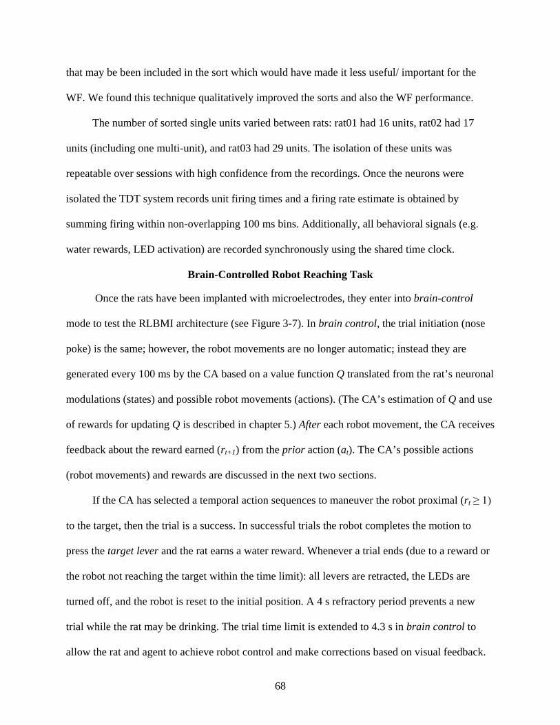
68

that may be been included in the sort which would have made it less useful/ important for the

WF. We found this technique qualitatively improved the sorts and also the WF performance.

The number of sorted single units varied between rats: rat01 had 16 units, rat02 had 17

units (including one multi-unit), and rat03 had 29 units. The isolation of these units was

repeatable over sessions with high confidence from the recordings. Once the neurons were

isolated the TDT system records unit firing times and a firing rate estimate is obtained by

summing firing within non-overlapping 100 ms bins. Additionally, all behavioral signals (e.g.

water rewards, LED activation) are recorded synchronously using the shared time clock.

Brain-Controlled Robot Reaching Task

Once the rats have been implanted with microelectrodes, they enter into brain-control

mode to test the RLBMI architecture (see Figure 3-7). In brain control, the trial initiation (nose

poke) is the same; however, the robot movements are no longer automatic; instead they are

generated every 100 ms by the CA based on a value function Q translated from the rat’s neuronal

modulations (states) and possible robot movements (actions). (The CA’s estimation of Q and use

of rewards for updating Q is described in chapter 5.) After each robot movement, the CA receives

feedback about the reward earned (rt+1) from the prior action (at). The CA’s possible actions

(robot movements) and rewards are discussed in the next two sections.

If the CA has selected a temporal action sequences to maneuver the robot proximal (rt ≥ 1)

to the target, then the trial is a success. In successful trials the robot completes the motion to

press the target lever and the rat earns a water reward. Whenever a trial ends (due to a reward or

the robot not reaching the target within the time limit): all levers are retracted, the LEDs are

turned off, and the robot is reset to the initial position. A 4 s refractory period prevents a new

trial while the rat may be drinking. The trial time limit is extended to 4.3 s in brain control to

allow the rat and agent to achieve robot control and make corrections based on visual feedback.

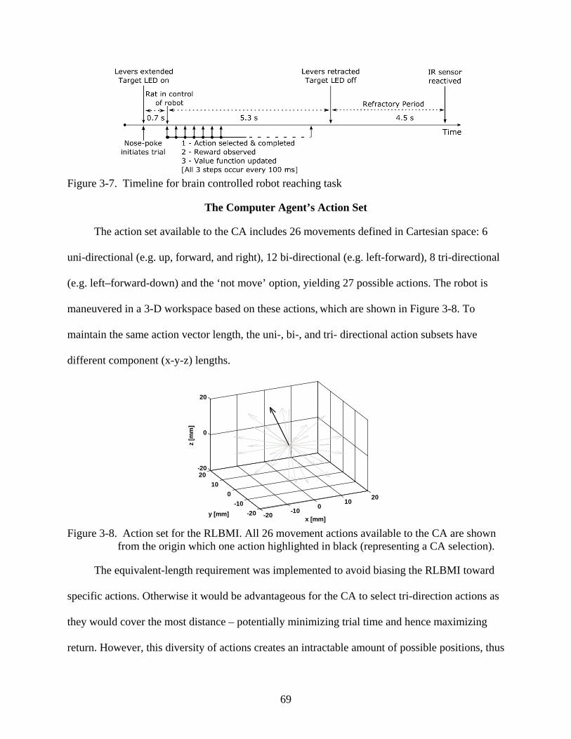
69

Figure 3-7. Timeline for brain controlled robot reaching task

The Computer Agent’s Action Set

The action set available to the CA includes 26 movements defined in Cartesian space: 6

uni-directional (e.g. up, forward, and right), 12 bi-directional (e.g. left-forward), 8 tri-directional

(e.g. left–forward-down) and the ‘not move’ option, yielding 27 possible actions. The robot is

maneuvered in a 3-D workspace based on these actions, which are shown in Figure 3-8. To

maintain the same action vector length, the uni-, bi-, and tri- directional action subsets have

different component (x-y-z) lengths.

-20 -10 0 10 20

-20-10

010

20-20

0

20

x [mm]y [mm]

z [m

m]

Figure 3-8. Action set for the RLBMI. All 26 movement actions available to the CA are shown

from the origin which one action highlighted in black (representing a CA selection).

The equivalent-length requirement was implemented to avoid biasing the RLBMI toward

specific actions. Otherwise it would be advantageous for the CA to select tri-direction actions as

they would cover the most distance – potentially minimizing trial time and hence maximizing

return. However, this diversity of actions creates an intractable amount of possible positions, thus

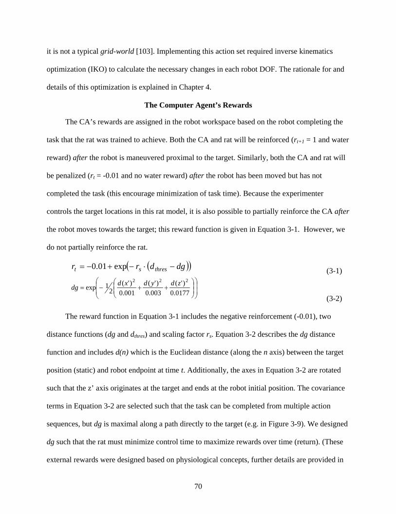
70

it is not a typical grid-world [103]. Implementing this action set required inverse kinematics

optimization (IKO) to calculate the necessary changes in each robot DOF. The rationale for and

details of this optimization is explained in Chapter 4.

The Computer Agent’s Rewards

The CA’s rewards are assigned in the robot workspace based on the robot completing the

task that the rat was trained to achieve. Both the CA and rat will be reinforced (rt+1 = 1 and water

reward) after the robot is maneuvered proximal to the target. Similarly, both the CA and rat will

be penalized (rt = -0.01 and no water reward) after the robot has been moved but has not

completed the task (this encourage minimization of task time). Because the experimenter

controls the target locations in this rat model, it is also possible to partially reinforce the CA after

the robot moves towards the target; this reward function is given in Equation 3-1. However, we

do not partially reinforce the rat.

( )( )dgdrr thresst −⋅−+−= exp01.0 (3-1)

++−=

0177.0)'(

003.0)'(

001.0)'(

21exp

222 zdydxddg (3-2)

The reward function in Equation 3-1 includes the negative reinforcement (-0.01), two

distance functions (dg and dthres) and scaling factor rs. Equation 3-2 describes the dg distance

function and includes d(n) which is the Euclidean distance (along the n axis) between the target

position (static) and robot endpoint at time t. Additionally, the axes in Equation 3-2 are rotated

such that the z’ axis originates at the target and ends at the robot initial position. The covariance

terms in Equation 3-2 are selected such that the task can be completed from multiple action

sequences, but dg is maximal along a path directly to the target (e.g. in Figure 3-9). We designed

dg such that the rat must minimize control time to maximize rewards over time (return). (These

external rewards were designed based on physiological concepts, further details are provided in

71

Appendix A.) The target proximity threshold dthres sets the necessary value of dg to complete a

task (rt ≥ 1) and can be adjusted from close to the robot starting position to far away as a

mechanism to shape complex behaviors. Finally, rs controls the distribution of partial

reinforcements that can be given to further develop the rat’s control. This set of parameters for

rewards formalizes the goals of the task.

Figure 3-9. Sequence of action selections to reach a reward threshold. The robot position at each

time step is unknown to the BMI agent but visible to the rat (target lever is marked by the diamond). Both the possible actions at each step (light gray) and the selected action (black) are shown. Once the robot position crosses the dg threshold (the gray Gaussian), the trial is considered a success (more details in Figure 3-7).

Equation 3-1 naturally invites objections from experienced BMI designers because rt is a

scalar proximity metric. All necessary information to evaluate rt is available from the robot and

target positions at time t. This fuels suspicion that the CA is being trained as a proximity detector

which reduces it to supervised learning (in 1D). However, Equations 3-1 and 3-2 describes the

reward for the CA and not the training method of the CA. Earlier in the section, we clearly stated

that this reward is provided to the CA after an action/ task is completed.

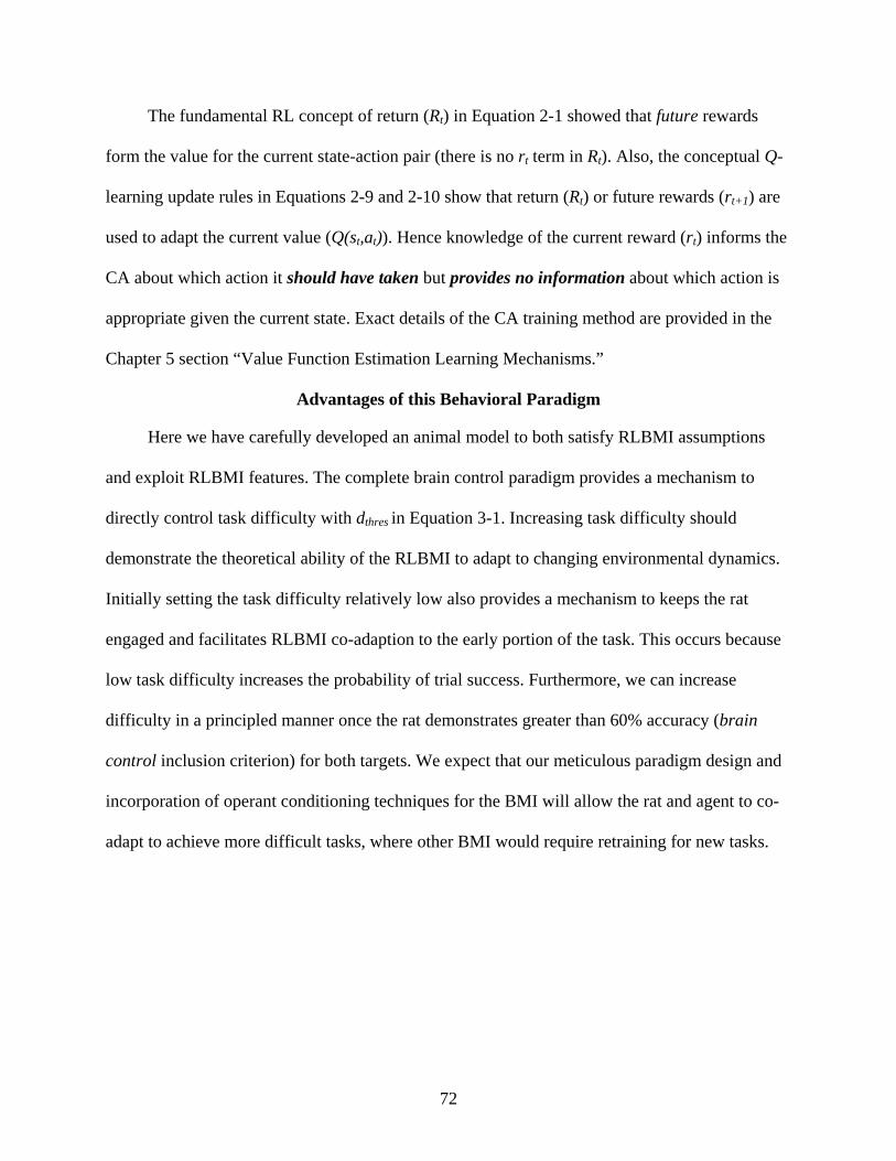
72

The fundamental RL concept of return (Rt) in Equation 2-1 showed that future rewards

form the value for the current state-action pair (there is no rt term in Rt). Also, the conceptual Q-

learning update rules in Equations 2-9 and 2-10 show that return (Rt) or future rewards (rt+1) are

used to adapt the current value (Q(st,at)). Hence knowledge of the current reward (rt) informs the

CA about which action it should have taken but provides no information about which action is

appropriate given the current state. Exact details of the CA training method are provided in the

Chapter 5 section “Value Function Estimation Learning Mechanisms.”

Advantages of this Behavioral Paradigm

Here we have carefully developed an animal model to both satisfy RLBMI assumptions

and exploit RLBMI features. The complete brain control paradigm provides a mechanism to

directly control task difficulty with dthres in Equation 3-1. Increasing task difficulty should

demonstrate the theoretical ability of the RLBMI to adapt to changing environmental dynamics.

Initially setting the task difficulty relatively low also provides a mechanism to keeps the rat

engaged and facilitates RLBMI co-adaption to the early portion of the task. This occurs because

low task difficulty increases the probability of trial success. Furthermore, we can increase

difficulty in a principled manner once the rat demonstrates greater than 60% accuracy (brain

control inclusion criterion) for both targets. We expect that our meticulous paradigm design and

incorporation of operant conditioning techniques for the BMI will allow the rat and agent to co-

adapt to achieve more difficult tasks, where other BMI would require retraining for new tasks.

73

CHAPTER 4 IMPLEMENTING A REAL-TIME BRAIN MACHINE INTERFACE

Introduction

The behavioral paradigm was carefully designed to provide an animal model of the

complete RLBMI architecture [86]. Specifically, the paradigm respects all of the RLBMI

assumptions but also showcases novel features of the RLBMI. The computational portion (CA)

of the RLBMI had already shown promising ability to generalize and complete different tasks in

offline simulations [120]. According to our design and prior BMI literature [64], completing the

feedback loop and testing the system online should only improve performance. All of the pieces

had come together and there was great excitement to demonstrate this system to the world!

But as the old saying goes, the devil was in the details. The most critical issue for this

closed-loop was meeting the real-time execution deadlines. Unlike the simulations, it was

important to generate BMI output within a set time to provide user feedback. Furthermore, only

limited computing power and memory was available (at that time) for acquiring neural data

through the TDT recording hardware, evaluating/ training the RLBMI networks, controlling the

behavioral paradigm, visualizing RLBMI performance, and controlling the robot. Finally, all

processing had to be done in a Windows operating system because TDT is not compatible with

any other (e.g. real-time) operating systems. Unforgiving time constraints were excellent

motivators to distill what is necessary in a BMI control from what seems elegant or ideal.

To demonstrate this BMI, each computational component was optimized for efficiency.

This systematic optimization also helped create a Cyber Workstation (C-W) as a by-product. The

C-W provides tremendous remote computing power yet can still return BMI outputs locally to

satisfy real-time deadlines. This not only alleviates the need for RLBMI optimization, it

redefines the future of BMI design because developers will only be limited by their imagination.

74

Real-Time Performance Deadlines

The RLBMI architecture assumes the rat receives feedback for each of his neuro-

modulations in the form of robot actions (see Figure 2-5). Behaviorist theory states that the rat’s

ability to associate feedback with behavior is a function of repeatability and delays [119, 121].

As we observed with the automated rat training (Chapter 3), the highest probability of

association results from consistent and prompt feedback. This motivates the real-time

performance deadlines of the RLBMI – provide consistent feedback as soon as possible.

The lower-bound on these performance deadlines was estimation of the neuronal FR.

Online spike-sorting for all 32 electrodes is performed via the TDT recording hardware. When

an action potential was detected for an identified neuron, the counter for that neuron was

incremented. Every 100 ms these counter values were saved, multiplying them by ten yields the

estimated1 FR in Hz. Hence, a new state is only available to the CA every 100 ms. The RLBMI

real-time processing is defined as requiring the following processes to be completed between

consecutive states: (items in boldface are either computationally or physically time-intensive)

• Neural signal acquired and pre-processed • All state-action values estimated • Policy evaluated (select an action) • Inverse kinematics to convert Cartesian actions to robot joint commands • Safety tests to protect the rat, hardware, and experimenter • Robot must physically move to complete action • Observation of the CA reward • Value iteration based on the reward

RLBMI Algorithm Implementation

The first step toward meeting these deadlines was to reorganize the CA algorithm for

closed-loop control. The offline simulations had worked brilliantly; however, there were

1 Estimated FR is averaged over 100 ms to be consistent with prior work and peers in BMI. Using different averaging has been suggested but Carmena [59] and Kim [60] found no significant effects on in BMI performance.

75

advantages of being offline which were previously unrealized. In the absence of time constraints,

the value function estimation (VFE) networks could be trained over night, analyzed, and then

tested in novel data. Everything was integrated in Matlab with unique functions for training,

analyzing, and testing the RLBMI. Due to familiarity, I initially developed a closed-loop RLMBI

in Matlab. However, early testing showed Matlab was at least an order of magnitude slower than

Visual C++ for communicating with TDT hardware and the robot controller. Additionally, the

variance in communication times was an order of magnitude higher. Finally, Matlab was not as

capable of providing large, stable memory allocations for variables as C++.

To meet the computational deadlines and have sufficient memory for variables, it was

necessary to translate the Matlab code to C++. Furthermore, it would be beneficial to quickly

transition between RLBMI training (if necessary) and co-adaptive control with analysis

constantly available. This was achieved by combining the separate Matlab functions into

methods which were available to the single RLBMI controller class. Using a switch statement

and a few flags, the RLBMI could progress between three phases of closed-loop control as

necessary without redundant processing or memory allocation. The three phases are:

1. Training data acquisition and processing (if necessary) 2. VFE network pre-training (if necessary) 3. Closed-loop robot control

Typically only the 3rd phase is necessary as the network parameters are saved from prior

session or the rat is given a random set of VFE weights and learns on the fly. However, this

segmentation allows the experimenter to complete the entire training procedure within a single

session without removing the rat (ideally also with minimal delays). Additionally, limited

RLBMI analysis is provided throughout all phases as feedback for the experimenters. Detailed

flowcharts of phases 1 & 2 are shown in Figure 4-1 and phase 3 is shown in Figure 4-2

76

Figure 4-1. RLBMI algorithm phases 1 and 2. Phase 1 (left) includes all preprocessing steps to acquire neural data, detect when trials have occurred, and save this data for further processing. Phase 2 (right) partitions the data from Phase 1 into training and test segments, trains N VFE networks serially, and then saves the optimal VFE network.

77

Figure 4-2. Phase 3 of the RLBMI algorithm. This phase provides closed loop control and is typically used exclusively. The main branches account for the different robot behaviors at the end of a trial, i.e. the robot automatically resetting to the initial position. Additionally, performance information is updated at the end of each trial.

78

Recording Hardware Architecture Parallelization

Once the RLBMI algorithms were translated to and optimized in C++ only two major

obstacles remained – data acquisition and robot control. Prior closed loop SL BMI had been

demonstrated with similar TDT hardware and the same computer in 2005 via Matlab (Sanchez,

unpublished). However, the added complexity of the RLBMI paradigm in the TDT hardware and

overall computational burden created a problem. The time required to acquire neural data from

the TDT storage buffers consumed up to 80% of the computing budget (Matlab or C++). Also,

the RLBMI could not always detect that new neural data (states) were available2.

The problem’s root cause was not the delay in polling any particular buffer but the additive

delays and variances in polling 32 buffers sequentially. To overcome this problem, the TDT

recording hardware’s control logic was redesigned such that it could process and store the neural

data in parallel. Also, a new index buffer structure was created which could be polled less

frequently but reliably updated the RLBMI that new neural data was available. Table 4-1 details

the improved performance of the redesigned control logic. The average data acquisition time

decreases by an order of magnitude. On average only 3% of the computing budget is used for

data acquisition. The RLBMI has more free time for other processes and no longer misses states.

Table 4-1. Neural data acquisition time for serial vs. parallel TDT control logic Recording

Architecture Mean Standard

Deviation Maximum

Serial 20.60 ms 14.89 ms 81.39 ms Parallel 2.70 ms 5.59 ms 46.41 ms

Robot Control via Inverse Kinematics Optimizations

The final remaining obstacle was to advance from simulating robot arm endpoint positions

(offline) to actually applying the necessary differential commands to each robot joint (see Figure

2 This is necessary for synchronization because the RLBMI code and TDT hardware operate on different clocks.

79

4-3) to achieve those movements (online). Determining the appropriate differential commands

requires inverse kinematics/ dynamics [133]. The inverse kinematics calculation for a redundant

four degree-of-freedom (DOF) robot3 does not have a unique closed form solution because there

is not a unique mapping from endpoint to joint angles [133]. Initially I thought to use an

optimization but dismissed it as a ‘non-principled’ solution. Instead I tried deriving the equations

to find the non-unique set of solutions which could satisfy the inverse kinematics requirement. I

reasoned that the equations would be evaluated quickly and provide a manifold of solutions but

failed to consider that this solution would still need an optimization on the back-end. After many

pages of trigonometry and equation substitutions, I still could not find a solution set. I asked an

expert in mechanics (BJ Fregly) for advice and he immediately suggested using an optimization.

Figure 4-3. Dynaservo miniCRANE robot.

Inverse Kinematics Optimization (IKO) will find a set of joint angles which will achieve

the movement. A sequential quadratic programming algorithm (Matlab’s fmincon) was used in

the IKO due to the robotic constraints (e.g. max operating speed, safe joint positions). This IKO

3 The miniCRANE robot has 5 possible DOF, however only 4 DOF are used in the RLBMI. The 5th DOF (U-axis) rotates the endpoint but does not affect the endpoint position.

80

yields an appropriate set of DOF commands for each action given the current joint angles

(computation time ~25 ms). The 26 different actions4 from any robot position create thousands

of unique possible robot locations (example in Figure 4-4). Any look-up table mapping the

necessary commands for each DOF would be unfeasibly large. Computing the IKO in real-time

is also undesirable because it consumes more than a quarter of the RLBMI computing budget.

Furthermore, the IKO is not guaranteed to generate an optimal solution – error checking and

additional IKO further consume the computing budget.

Figure 4-4. Possible IKO starting positions. Each random walk selected an action approximately

10,000 times and here are the initial positions for action L. The empty space (y > 0.22 & z < 0.2) is the area where the robot physically can not reach. Axes are in meters.

Creating surrogate models of IKO can overcome the issues discussed above. The surrogate

models perform system identification where the plant is the IKO (see Figure 4-5). A set of 26

MLPs (one for each action) are used to model the IKO. The MLP inputs are 4 robot joint angles,

which are normalized based on the training set statistics using the NeuroSolutions’ technique

(bounded between +/-0.9) because it is less dependant on the data statistics relative to the zero-

mean, unit-variance normalization. Each MLP has bias terms, 50 hyperbolic tangent PEs in the

hidden layer (based on generalization results), and 4 linear output PE. 4 As described in Ch 3, the uni-, bi-, and tri- directional action subsets have different component (x-y-z) lengths.

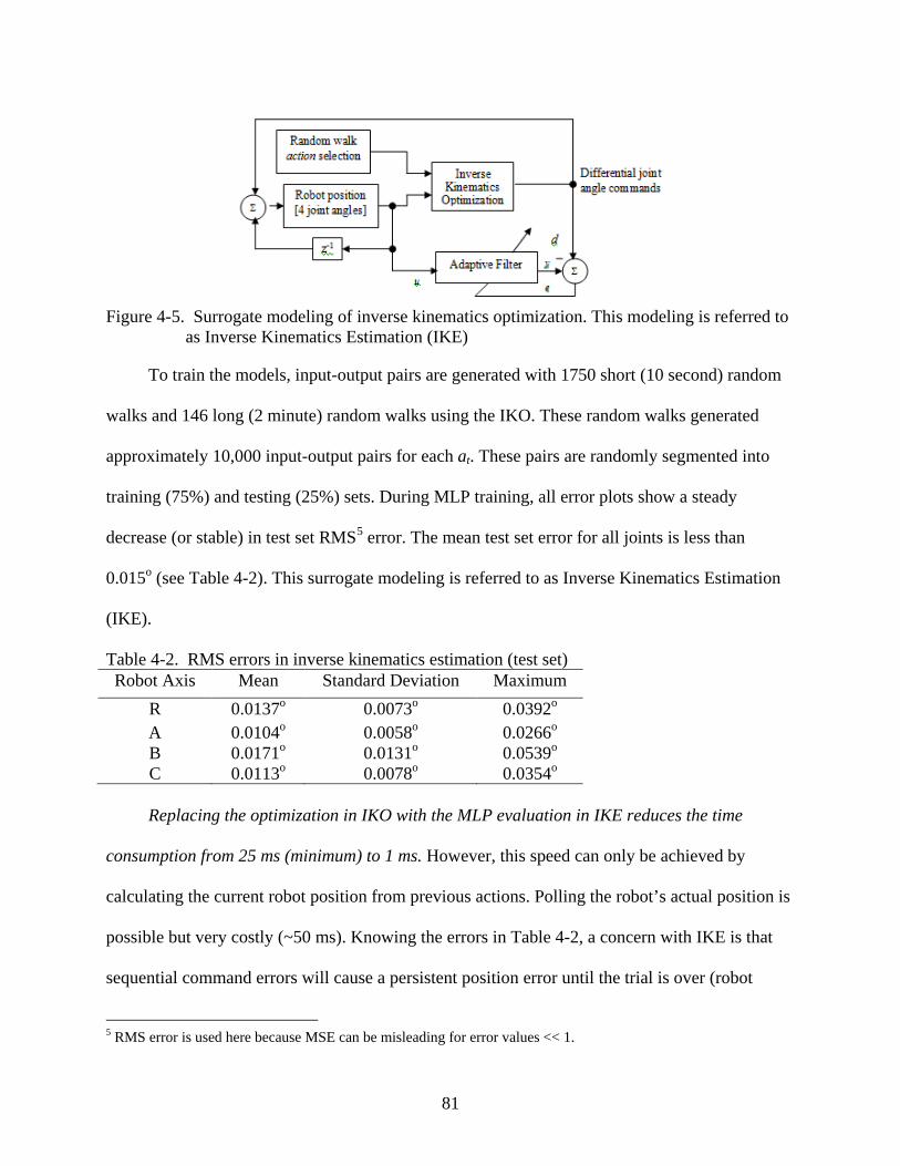
81

Figure 4-5. Surrogate modeling of inverse kinematics optimization. This modeling is referred to

as Inverse Kinematics Estimation (IKE)

To train the models, input-output pairs are generated with 1750 short (10 second) random

walks and 146 long (2 minute) random walks using the IKO. These random walks generated

approximately 10,000 input-output pairs for each at. These pairs are randomly segmented into

training (75%) and testing (25%) sets. During MLP training, all error plots show a steady

decrease (or stable) in test set RMS5 error. The mean test set error for all joints is less than

0.015o (see Table 4-2). This surrogate modeling is referred to as Inverse Kinematics Estimation

(IKE).

Table 4-2. RMS errors in inverse kinematics estimation (test set) Robot Axis Mean Standard Deviation Maximum

R 0.0137o 0.0073o 0.0392o A 0.0104o 0.0058o 0.0266o B 0.0171o 0.0131o 0.0539o C 0.0113o 0.0078o 0.0354o

Replacing the optimization in IKO with the MLP evaluation in IKE reduces the time

consumption from 25 ms (minimum) to 1 ms. However, this speed can only be achieved by

calculating the current robot position from previous actions. Polling the robot’s actual position is

possible but very costly (~50 ms). Knowing the errors in Table 4-2, a concern with IKE is that

sequential command errors will cause a persistent position error until the trial is over (robot

5 RMS error is used here because MSE can be misleading for error values << 1.

82

resets to a known position). Figure 4-6 shows a single trial from step 800 to step 900. Three large

(> 10 mm) command errors at steps 868, 881, and 887 cause the position error to be > 50 mm

from step 868 on. As expected, command error propagates through the trial. Hence, trial length

affects position error (see Figure 4-7) and should be upper-bounded if IKE is used.

800 810 820 830 840 850 860 870 880 890 900

-200

-150

-100

-50

0P

ositi

on E

rror [

mm

]

800 810 820 830 840 850 860 870 880 890 900-80

-60

-40

-20

0

Time [100ms]

Com

man

d E

rror [

mm

]

xyz

Figure 4-6. Inverse kinematics estimation error accumulation. IKE command errors at each

time-step (bottom) propagate to robot endpoint position errors (top)

5 10 15 20 25 30

-0.2

-0.1

0

Mea

n co

mm

and

erro

r [m

m] Command error vs. Trial length [action #1]

5 10 15 20 25 30

2

4

6

8

10

Max

com

man

d er

ror [

mm

]

Trial length [s]

xyz

5 10 15 20 25 30

-4-3-2-101

Mea

n co

mm

and

erro

r [m

m] Co a d e o s a e gt [act o # ]

5 10 15 20 25 30

5

10

15

20

25

30

Max

com

man

d er

ror [

mm

]

Trial length [s]

xyz

Figure 4-7. Accumulating position error vs. trial length. Mean (top) and maximum (bottom) IKE

errors are shown for the best (left) and worst (right) modeled actions.

Development of a Cyber Workstation

Although the BMI implementation challenges were overcome, it required extensive

optimizations (algorithms and recording hardware) and approximations (IKE). These steps took

months to complete and limited the complexity of possible robot actions, maximum trial lengths,

83

and position accuracy. It was clear that these present challenges are a bottleneck to BMI design

and implementation. Through collaboration with the Advanced Computing and Information

Systems (ACIS) lab, we have developed a grid computing architecture as a test-bed for BMI

research [134, 135]. Specifically, the Dynamic, Data Driven Adaptive Systems (DDDAS) BMI

project (DDDBMI) at UF has developed a Cyber-Workstation (C-W). This C-W can provide

tremendous resources due to the speed of individual computers within the grid and parallel grid

computing.

Guiding the design of the C-W was an interesting process because it went against all the

design experience of implementing the RLBMI. Instead of working within known computational

power and storage constraints, the PI on the DDDBMI project told me to just dream of whatever

resources the neuroscience and BMI communities would ever want in a BMI. This request was

staggering in scope, but the C-W was designed with the unlimited resources philosophy in mind.

The obvious design requirement is for the C-W to meet the real-time processing

requirements. Each BMI developer will have unique needs due to their user, algorithms, and

prosthetics. However the necessity of real-time feedback in a closed-loop BMI is universal.

Before developing any BMI-specific resources, we developed the communication infrastructure

of the C-W. Neuro-physiological data is acquired from the rat via TDT hardware at the

Neuroprosthetics Research Group (NRG) lab. Local software (which interfaces with the C-W),

extracts the neuro-physiological data and sends it (~500 m) to the ACIS lab for processing. At

the ACIS lab there is a grid of computers to process the data and then send the necessary BMI

feedback (robot control commands) back to NRG within the 100 ms.

The next design requirement addressed neuroscience. Although not classically trained, I

was familiar with a subset of neuroscience literature. The neuroscientists I knew were not

84

terribly interested in writing algorithms. However, my general impression was that a subset of

the community had to contend with mountains of neuro-physiological data, needed to preprocess

this data, and then perform potentially complex statistical tests to make sense of it. To serve

neuroscience, we decided that the C-W should have a library (toolbox) of established data

processing/ evaluation techniques that could be used without developing them from scratch.

Additionally, a visualization feature would provide real-time feedback to the neuroscientists as

their experiments ran. Finally, the C-W would provide data warehousing.

The BMI community has the same appetite for processing power, visualization ability, and

data warehousing as the neuroscientists. BMI developers typically code their own algorithms, but

would probably also appreciate a toolbox of established components to construct their BMI. The

problem with developers is that each has their own style. We needed to establish a C-W platform

that was flexible enough to incorporate custom algorithms but had a known structure. Providing

structure preserved the communication backbone of the C-W and allowed for automation in

requesting more computing power.

Still inspired by Wolpert and Kawato’s MPFIM theory of motor control [16], we decided

that this was a reasonable C-W structure for BMI development. Figure 4-8 shows our

interpretation of the MPFIM architecture. Beyond its merits as a motor control theory, the

architecture seemed a good fit for the C-W because it can exploit grid-computing to process the

multiple model-pairs in parallel and has access to all of these model-pairs to aggregate the

results. Furthermore, it provides vast expandability to BMI designers. For example, the RLBMI

can be interpreted as a MPFIM architecture where the IKE is an inverse model, the current robot

position is calculated by a forward model, and the Q is calculated by a responsibility predictor

model. There are 27 groups of these models, one group for each possible action. The CA acts as

85

the responsibility estimator and decides which group of models to use (selects an action). In the

current RLBMI, the forward models are look-up tables and the inverse models are MLP

evaluations. But there is nothing that limits future designers from expanding any of these models

– all they need to do is develop algorithms within the appropriate block in Figure 4-10. On the

other end of the spectrum, BMI designers who do not want this structure can still develop a

single input – single output type of BMI by just developing a single model and leaving the rest of

the model pairs empty.

Figure 4-8. BMI adaptation of the multiple paired forward-inverse models for motor control.

A prototype C-W achieved limited closed-loop BMI control in 2007 (DiGiovanna et al.

unpublished). The rat exercised mechanical control over the cage levers, while the Cyber-

Workstation decoded the rat neural signals to control the robot arm via linear models trained

with the RLS algorithm [134]. This demonstrated the novel ability to adapt a BMI in real-time

using computation resources at a different location. Other researchers have since performed a

similar remote adaption but across the globe [136].

Currently, the C-W is capable of running the entire RLBMI algorithms online (Zhao et. al,

unpublished) and also performing off-line analysis and training. Current C-W developers are

86

constantly working to add features, e.g. the ability to incorporate Matlab code (Matlab is a very

popular development platform). A modest example of the computational power is shown in

Figure 4-9 for a real world problem of initializing a RLBMI. It dramatically outperforms local

resources using three Virtual Machines (VMs), at least ten VMs are currently available and this

number is expandable. Although still in the simulation stages, the initialization time is reduced

by a factor of 11 if VMs are fully exploited. This is important because we are now approaching

the ability to fully initialize the CW between normal trials! For the first session of Rat 3, the

minimum and average inter-trial times were 1:06 and 2:12 respectively. Using 18 simulated

VMs, the entire network initialization time was 1:26. We could theoretically train the RLBMI

network without the rat even noticing the delay. However, there remains the issue of collecting

the necessary number of trials (the lower bound here is unknown) to provide training data.

2 4 6 8 10 12 14 16 18

200

400

600

800

1000

1200

1400

1600

1800

2000

2200RLBMI Initialization Time for Rat #3

Com

puta

tion

Tim

e [s

]

Number of Virtual Machines Used

CyberWorkstation ResultCyberWorkstation SimulationLaptop (Local)

Figure 4-9. Basic comparison of the C-W and local computing. This is the time require to

initialize the RLBMI using the real data from rat 3. Already with 3 modules (VMs) the C-W is faster. Additionally, the local computer is free for other processing tasks.

87

Finally, the Cyber-Workstation provides an integrated research platform for multiple

remote users to design and implement BMI paradigms and then facilitate repeatable analysis of

these BMIs. The current incarnation of the C-W is shown in Figure 4-11.

88

Figure 4-10. Complexity and expandability of the C-W. BMI developers can ‘plug-in’ their own code to any of the boxes

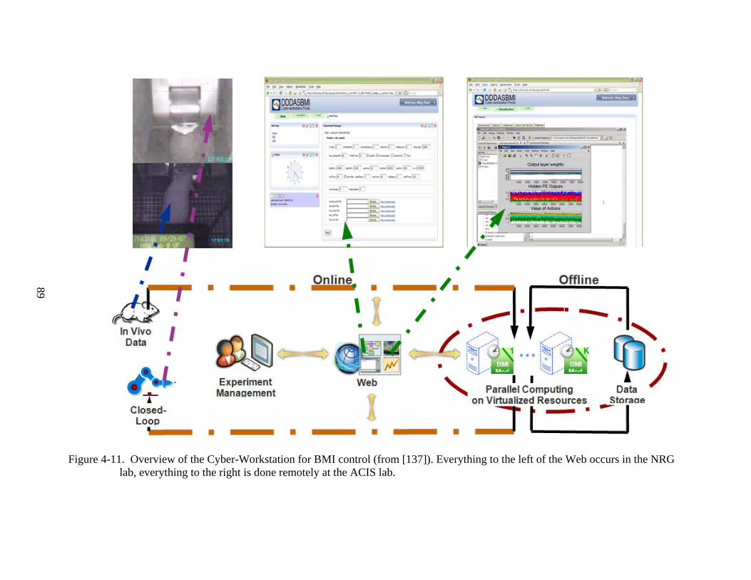
89

Figure 4-11. Overview of the Cyber-Workstation for BMI control (from [137]). Everything to the left of the Web occurs in the NRG lab, everything to the right is done remotely at the ACIS lab.

90

CHAPTER 5 CLOSED-LOOP RLBMI PERFORMANCE

Introduction

In the prior chapters, we have developed both a computational architecture and in vivo

BMI experimental paradigm to show the performance of a RLBMI in goal directed reaching

tasks that parallel a paralyzed patient’s goal of controlling a prosthetic. Through offline

simulations, we proved that the RLBMI conceptually could control a BMI. Finally, after

systematic optimization of each processing component it became feasible to implement the

RLBMI in closed-loop control. Even with insight from simulations, a few challenges remained:

• Which mechanisms should be employed to approximate value? • How to overcome the known slow training of RL? • How to manage the large RLBMI parameter set? • How to effectively demonstrate the utility of co-adaptation? • How to quantify the RLBMI performance?

As in many things, there was no free lunch [138] – each challenge involved trade-offs. For

example, the designer must set a balance between maintaining stable control and encouraging

‘minimum cost’ action selection strategies. Also, it was difficult not to project onto the rats, e.g.

the experimenter knew the ‘optimal’ strategy and how the rat should be thinking. Avoiding this

anthropomorphism was critical; otherwise the experimenters would spend a lifetime waiting for

the rats to behave like humans.

We also could not extract many closed-loop and co-adaptive BMI implementation

techniques from the literature. To our knowledge, Gage et al. had the only similar closed-loop,

brain-control study however, it was a SL framework [98]. Perhaps the most difficult challenge

was requests to quantify RLBMI performance in SL concepts. Though obviously ill-posed, the

prevalent idea is SL and it is difficult to convince and relate to others only familiar with that SL

framework. Here we focus on BMI performance metrics; RL metrics are addressed in Chapter 6.

91

Approximating the RLBMI State-Action Value

Assigning a value to each possible action given the current state is fundamental to RL

[103]. It enables the agent to perform value and/ or policy iteration to learn action selection

strategies which maximize reward. In Chapter 2, we applied dimensionality reduction to the

neural state with the goal of finding a limited state set to facilitate storing the state-action value

function Q (see Equation 2-2) in a look-up table [103]. This could simplify value estimation –

requiring only one addition and multiplication to update each state-action pair using the most

basic RL techniques. This simplicity can be critical for BMI implementation. The Advanced

Robotics Technology & Systems lab (Scuola Superiore Sant’Anna) has developed a

sophisticated cyber-hand [139, 140] for amputees. Mechanically, this prosthetic is amazingly

realistic with control based on human physiology (i.e. tendons). However, colleagues at the

ARTS lab lament that there is no BMI control algorithm for it. Part of the reason is that the

control must be robust and simple such that it can be achieved in implanted, low-power DSPs.

Paradoxically, this simplicity also expands the possible techniques for learning to estimate

Q. Colleagues at the Machine Learning Group (Cambridge University) are advancing the state of

the art in RL with techniques such as Gaussian process models for policy iteration [141] and

active learning through Bayesian RL [142]. They were very interested in the potential of RLBMI

and BMI in general as an application. Their more advanced techniques potentially can enhance

learning speed and accuracy in the RLBMI. However, like other techniques (e.g. decision-tree

methods, linear regressors) they scale poorly to high dimensional state-spaces and require (or

benefit from) segmentation, such as tiling, clustering, or hashing [103]. The RLBMI states were

48D, 51D, and 77D for rats 1, 2, and 3 respectively. High dimensional is subjective but typically

implies ≥ 10D; however, in some applications even 3D is considered high dimensional.

92

However, we found (in Chapter 2) that we could not use unsupervised preprocessing

segmentation to create a set of states. Furthermore, enumerating a state set based on possible

combinations of each RLBMI state vector component is intractable. Hence value function

estimation is a non-trivial task because it cannot be addressed with the well known basic set of

RL tools described in [103]. Instead of disjoint preprocessing, the RLBMI uses a neural network

to project the state to a space where segmentation is better performed – the hidden layer of a

neural network [120]. Through this complete neural network, established value estimation

techniques will be implemented.

Value Function Estimation Network Architecture

In [120] both single layer perceptrons (SLP) and multi-layer perceptrons (MLP) were

investigated for this architecture but MLPs exhibited both superior performance and required less

training data because they had fewer parameters. Adaptive-Critic architectures [143] were also

investigated but dismissed due to the number of parameters and similar performance of Actor-

Critic to the MLP. The RLBMI uses a gamma delay line [122] (K = 3, µ = 0.3333) to embed 600

ms of neuronal modulation history into the state. This further reduces parameters but respect the

Markov assumptions of RL. Then a MLP both segments the state (in the hidden layer) and

estimates Q (in the output layer) as:

( )∑∑ ∑ ⋅=

=

jjktj

jjkij

ititk wsnetwwssQ ,tanh)(

(5-1)

Each output processing element (PE) represents the value of the kth action given the state

vector. Each state vector component1 is normalized based on observed FRs using the

NeuroSolutions’ technique [144] (bounded between +/-0.9) because we found it more robust to

1 The recorded neural FRs were normalized. It follows that their gamma histories were also bounded by +/- 0.9

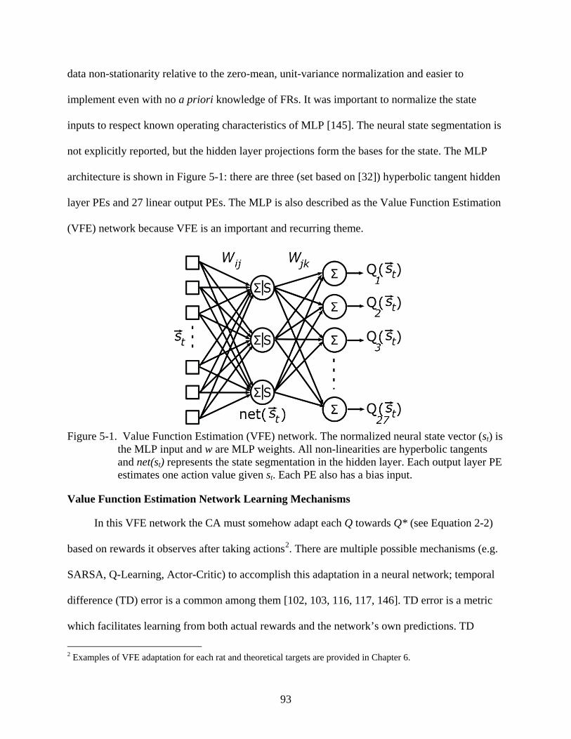
93

data non-stationarity relative to the zero-mean, unit-variance normalization and easier to

implement even with no a priori knowledge of FRs. It was important to normalize the state

inputs to respect known operating characteristics of MLP [145]. The neural state segmentation is

not explicitly reported, but the hidden layer projections form the bases for the state. The MLP

architecture is shown in Figure 5-1: there are three (set based on [32]) hyperbolic tangent hidden

layer PEs and 27 linear output PEs. The MLP is also described as the Value Function Estimation

(VFE) network because VFE is an important and recurring theme.

Figure 5-1. Value Function Estimation (VFE) network. The normalized neural state vector (st) is

the MLP input and w are MLP weights. All non-linearities are hyperbolic tangents and net(st) represents the state segmentation in the hidden layer. Each output layer PE estimates one action value given st. Each PE also has a bias input.

Value Function Estimation Network Learning Mechanisms

In this VFE network the CA must somehow adapt each Q towards Q* (see Equation 2-2)

based on rewards it observes after taking actions2. There are multiple possible mechanisms (e.g.

SARSA, Q-Learning, Actor-Critic) to accomplish this adaptation in a neural network; temporal

difference (TD) error is a common among them [102, 103, 116, 117, 146]. TD error is a metric

which facilitates learning from both actual rewards and the network’s own predictions. TD

2 Examples of VFE adaptation for each rat and theoretical targets are provided in Chapter 6.

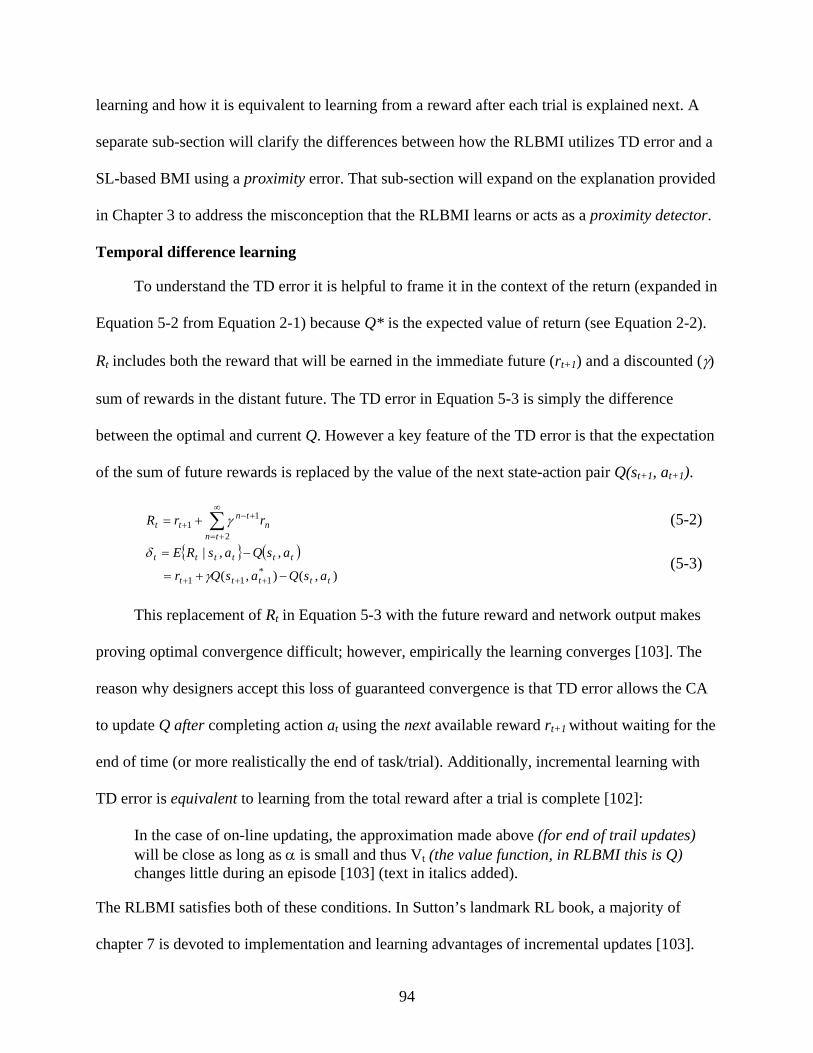
94

learning and how it is equivalent to learning from a reward after each trial is explained next. A

separate sub-section will clarify the differences between how the RLBMI utilizes TD error and a

SL-based BMI using a proximity error. That sub-section will expand on the explanation provided

in Chapter 3 to address the misconception that the RLBMI learns or acts as a proximity detector.

Temporal difference learning

To understand the TD error it is helpful to frame it in the context of the return (expanded in

Equation 5-2 from Equation 2-1) because Q* is the expected value of return (see Equation 2-2).

Rt includes both the reward that will be earned in the immediate future (rt+1) and a discounted (γ)

sum of rewards in the distant future. The TD error in Equation 5-3 is simply the difference

between the optimal and current Q. However a key feature of the TD error is that the expectation

of the sum of future rewards is replaced by the value of the next state-action pair Q(st+1, at+1).

∑∞

+=

+−+ +=

2

11

tnn

tntt rrR γ (5-2)

{ } ( )

),(),(

,,|*

111 ttttt

tttttt

asQasQr

asQasRE

−+=

−=

+++ γ

δ (5-3)

This replacement of Rt in Equation 5-3 with the future reward and network output makes

proving optimal convergence difficult; however, empirically the learning converges [103]. The

reason why designers accept this loss of guaranteed convergence is that TD error allows the CA

to update Q after completing action at using the next available reward rt+1 without waiting for the

end of time (or more realistically the end of task/trial). Additionally, incremental learning with

TD error is equivalent to learning from the total reward after a trial is complete [102]:

In the case of on-line updating, the approximation made above (for end of trail updates) will be close as long as α is small and thus Vt (the value function, in RLBMI this is Q) changes little during an episode [103] (text in italics added).

The RLBMI satisfies both of these conditions. In Sutton’s landmark RL book, a majority of

chapter 7 is devoted to implementation and learning advantages of incremental updates [103].

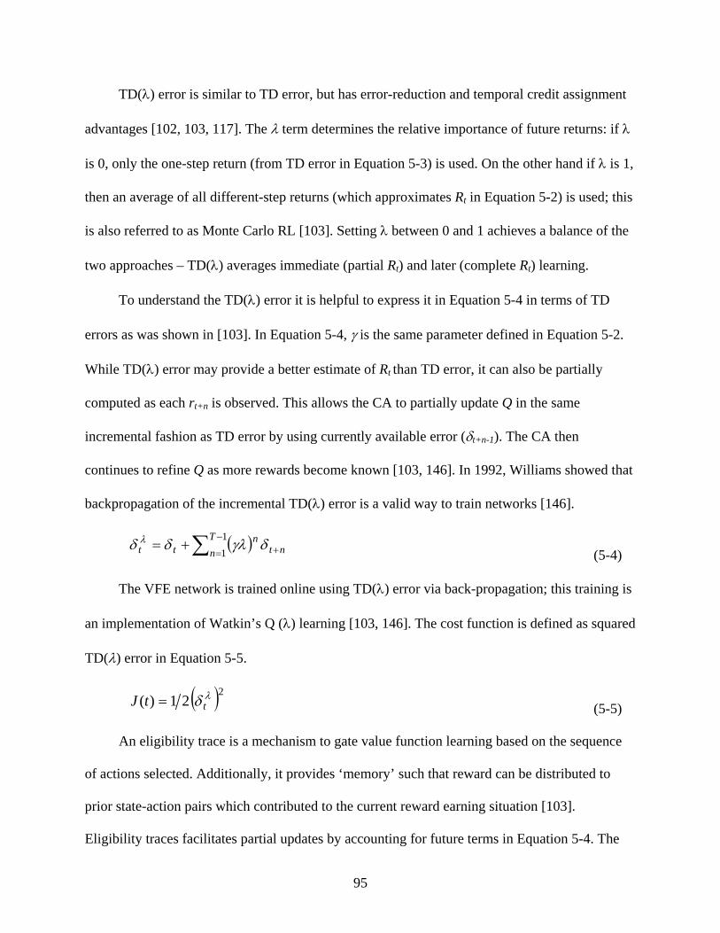
95

TD(λ) error is similar to TD error, but has error-reduction and temporal credit assignment

advantages [102, 103, 117]. The λ term determines the relative importance of future returns: if λ

is 0, only the one-step return (from TD error in Equation 5-3) is used. On the other hand if λ is 1,

then an average of all different-step returns (which approximates Rt in Equation 5-2) is used; this

is also referred to as Monte Carlo RL [103]. Setting λ between 0 and 1 achieves a balance of the

two approaches – TD(λ) averages immediate (partial Rt) and later (complete Rt) learning.

To understand the TD(λ) error it is helpful to express it in Equation 5-4 in terms of TD

errors as was shown in [103]. In Equation 5-4, γ is the same parameter defined in Equation 5-2.

While TD(λ) error may provide a better estimate of Rt than TD error, it can also be partially

computed as each rt+n is observed. This allows the CA to partially update Q in the same

incremental fashion as TD error by using currently available error (δt+n-1). The CA then

continues to refine Q as more rewards become known [103, 146]. In 1992, Williams showed that

backpropagation of the incremental TD(λ) error is a valid way to train networks [146].

( )∑ −

= ++=11

Tn nt

ntt δγλδδ λ

(5-4)

The VFE network is trained online using TD(λ) error via back-propagation; this training is

an implementation of Watkin’s Q (λ) learning [103, 146]. The cost function is defined as squared

TD(λ) error in Equation 5-5.

( )221)( λδ ttJ = (5-5)

An eligibility trace is a mechanism to gate value function learning based on the sequence

of actions selected. Additionally, it provides ‘memory’ such that reward can be distributed to

prior state-action pairs which contributed to the current reward earning situation [103].

Eligibility traces facilitates partial updates by accounting for future terms in Equation 5-4. The

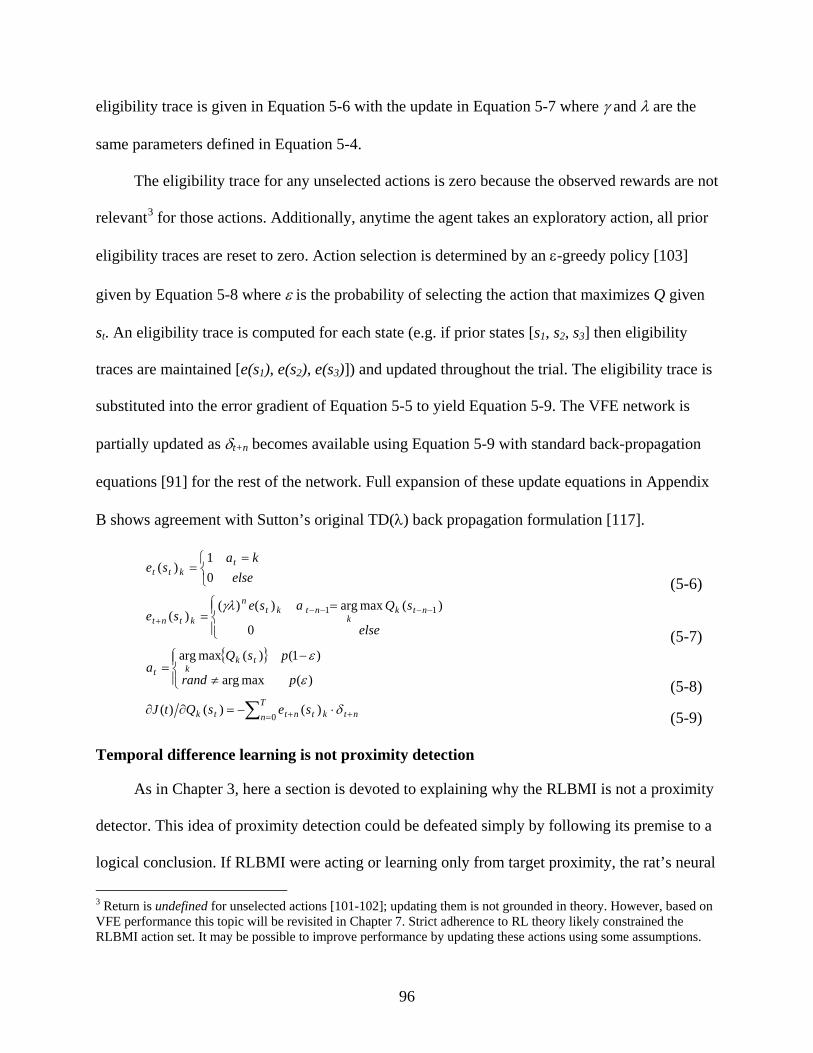
96

eligibility trace is given in Equation 5-6 with the update in Equation 5-7 where γ and λ are the

same parameters defined in Equation 5-4.

The eligibility trace for any unselected actions is zero because the observed rewards are not

relevant3 for those actions. Additionally, anytime the agent takes an exploratory action, all prior

eligibility traces are reset to zero. Action selection is determined by an ε-greedy policy [103]

given by Equation 5-8 where ε is the probability of selecting the action that maximizes Q given

st. An eligibility trace is computed for each state (e.g. if prior states [s1, s2, s3] then eligibility

traces are maintained [e(s1), e(s2), e(s3)]) and updated throughout the trial. The eligibility trace is

substituted into the error gradient of Equation 5-5 to yield Equation 5-9. The VFE network is

partially updated as δt+n becomes available using Equation 5-9 with standard back-propagation

equations [91] for the rest of the network. Full expansion of these update equations in Appendix

B shows agreement with Sutton’s original TD(λ) back propagation formulation [117].

=

=else

kase t

ktt 01

)( (5-6)

=

= −−−−+

else

sQasese ntk

kntkt

n

ktnt0

)(maxarg)()()( 11γλ

(5-7)

{ }

≠

−=

)(maxarg

)1()(maxarg

ε

ε

prand

psQa tk

kt

(5-8)

∑ = ++ ⋅−=∂∂Tn ntktnttk sesQtJ

0)()()( δ (5-9)

Temporal difference learning is not proximity detection

As in Chapter 3, here a section is devoted to explaining why the RLBMI is not a proximity

detector. This idea of proximity detection could be defeated simply by following its premise to a

logical conclusion. If RLBMI were acting or learning only from target proximity, the rat’s neural

3 Return is undefined for unselected actions [101-102]; updating them is not grounded in theory. However, based on VFE performance this topic will be revisited in Chapter 7. Strict adherence to RL theory likely constrained the RLBMI action set. It may be possible to improve performance by updating these actions using some assumptions.

97

modulations would be inconsequential and the robot would complete the task in every trial. None

of the simulations in Chapter 2 (e.g. Table 2-5 & Figure 2-6) showed perfect performance and

neither will any of the closed-loop results later in this chapter. However, the idea of proximity

detection is also unraveled by order of RLBMI operations or the mathematics of VFE updates.

The RLBMI follows a straightforward operating procedure, e.g. at time t:

1. Observe the neuronal state (st) 2. Estimate a value for each state-action pair (Q(st, at)) 3. Select the current action (at) based on Q(st, at) 4. Move the robot endpoint based on the selected action (at) The robot will be in a new position after completing this sequence; hence it is possible to

calculate the reward earned (rt+1). Also a new state will be available (because time = t+1) and the

prior Q function is updated at time t+1:

5. Calculate reward for the prior actions based on current proximity (rt+1) 6. Observe the current neuronal state (st+1) 7. Estimate a value for each current state-action pair (Q(st+1, at+1)) 8. Update4 the prior value Q(st, at) using TD error in Equation 5-3 The current reward signal (rt) is absent both from the operating procedure and any equations

contained therein. Instead, this reward (rt) only informs the CA about the utility of past actions

(at-1) but provides no information about which action (at) to take given the current state (st).

In order to create a proximity detector, these operating procedures would need to be

drastically revised, e.g. estimate future reward for all possible actions then select the action with

the highest estimated reward. Such revisions create a controller that does not learn (rt is not

adapted) and more importantly is not a BMI because the user (st) is not involved. We

confidently conclude that the RLBMI is not a proximity detector based on performance,

operating procedure, and VFE update equations.

4 The VFE network is actually trained with Equation 5-9 which follows the same TD error concept but is a more advanced learning method. However, neither Equation 5-9 nor Equation 5-3 use the current reward signal (rt)

98

Value Function Estimator Training

Although there were multiple other examples of adapting a MLP with TD(λ) error,

typically it requires either online training with a sufficiently large dataset or offline, batch-

training (repeatedly processing a smaller dataset) [103]. This feeds the common perception that

‘RL is too slow.’ Since one of the primary objectives was to facilitate user control of a BMI,

requiring extremely long training (or waiting) periods was not acceptable. Instead, the rat was

given immediate control of the robot before any training. This required starting online control

with random VFE network weights so that the rat controlled the robot immediately.

The robot trajectories were jerky due to the random Q but over multiple trials the rat and

CA co-adapted to reach at least one of the targets. Typically there was target selection bias due to

incomplete VFE adaptation5 (low α) or tracking (high α). However, offline batch-training

between the 1st and 2nd sessions6 resolved these issues. The VFE network was trained using the

initial session’s data with some crucial differences from the offline RLBMI simulations in

Chapter 2. The neural data is no longer segmented based on the rat’s behavior (this is not

possible in a causal and real-time system) – instead it includes all modulations within a trial.

Also, the CA rewards are defined as a function (see Equation 3-1) and all data was collected in

brain control. All trials (successes and failures) were used for training. A training set was created

from approximately 70% of the trials (30% reserved for a test set).

From the training data, the normalization coefficients were recorded for each neuronal unit

[144]; these coefficients remained static for all future sessions. Up to 20 different VFE network

were created, each with initial weights generated by a different random seed. Multiple networks

5 Setting VFE network learning rates and the other RLBMI parameters is discussed in the next section.

6 The 1st session had a random VFE and is not included in further analysis. The 2nd session is labeled session #1.

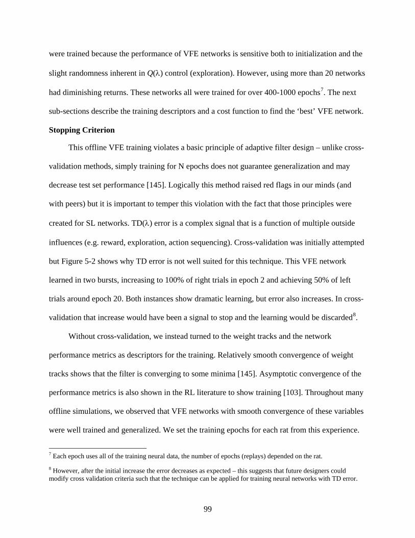
99

were trained because the performance of VFE networks is sensitive both to initialization and the

slight randomness inherent in Q(λ) control (exploration). However, using more than 20 networks

had diminishing returns. These networks all were trained for over 400-1000 epochs7. The next

sub-sections describe the training descriptors and a cost function to find the ‘best’ VFE network.

Stopping Criterion

This offline VFE training violates a basic principle of adaptive filter design – unlike cross-

validation methods, simply training for N epochs does not guarantee generalization and may

decrease test set performance [145]. Logically this method raised red flags in our minds (and

with peers) but it is important to temper this violation with the fact that those principles were

created for SL networks. TD(λ) error is a complex signal that is a function of multiple outside

influences (e.g. reward, exploration, action sequencing). Cross-validation was initially attempted

but Figure 5-2 shows why TD error is not well suited for this technique. This VFE network

learned in two bursts, increasing to 100% of right trials in epoch 2 and achieving 50% of left

trials around epoch 20. Both instances show dramatic learning, but error also increases. In cross-

validation that increase would have been a signal to stop and the learning would be discarded8.

Without cross-validation, we instead turned to the weight tracks and the network

performance metrics as descriptors for the training. Relatively smooth convergence of weight

tracks shows that the filter is converging to some minima [145]. Asymptotic convergence of the

performance metrics is also shown in the RL literature to show training [103]. Throughout many

offline simulations, we observed that VFE networks with smooth convergence of these variables

were well trained and generalized. We set the training epochs for each rat from this experience.

7 Each epoch uses all of the training neural data, the number of epochs (replays) depended on the rat.

8 However, after the initial increase the error decreases as expected – this suggests that future designers could modify cross validation criteria such that the technique can be applied for training neural networks with TD error.

100

Figure 5-2. Learning in a VFE network and TD error. The top plot shows task completion as the

network learns over multiple epoch. The bottom plots shows mean square TD error in the same network. The error initially increases when performance improves.

The weight tracks and training PR, TT, and δ show (noisy) convergence. Figure 5-3 shows

VFE weight adaptations for rat 3. The VFE network was trained using 105 trials for 1000

epochs. Figure 5-4 shows the corresponding Percentage of trials earning Reward (PR), Time to

reach Target (TT), and average TD error (δ) for each learning epoch. The average δ and TT

decreased and then stabilized, Additionally PR rapidly increased then stabilized; these training

results are representative all three rats. The VFE networks generalized for each rat.

Figure 5-3. Offline batch VFE training weight tracks. The top three plots each contain the

weights to one of the three hidden PEs. The bottom plot shows adaptation of the weights from the hidden PE outputs to the actions values at each output PE. This training was done for rat 3; it is representative of the other two rats.

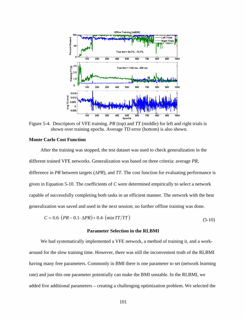
101

Figure 5-4. Descriptors of VFE training. PR (top) and TT (middle) for left and right trials is

shown over training epochs. Average TD error (bottom) is also shown.

Monte Carlo Cost Function

After the training was stopped, the test dataset was used to check generalization in the

different trained VFE networks. Generalization was based on three criteria: average PR,

difference in PR between targets (∆PR), and TT. The cost function for evaluating performance is

given in Equation 5-10. The coefficients of C were determined empirically to select a network

capable of successfully completing both tasks in an efficient manner. The network with the best

generalization was saved and used in the next session; no further offline training was done.

( ) ( )TTTTPRPRC min4.01.06.0 ⋅+∆⋅−⋅= (5-10)

Parameter Selection in the RLBMI

We had systematically implemented a VFE network, a method of training it, and a work-

around for the slow training time. However, there was still the inconvenient truth of the RLBMI

having many free parameters. Commonly in BMI there is one parameter to set (network learning

rate) and just this one parameter potentially can make the BMI unstable. In the RLBMI, we

added five additional parameters – creating a challenging optimization problem. We selected the

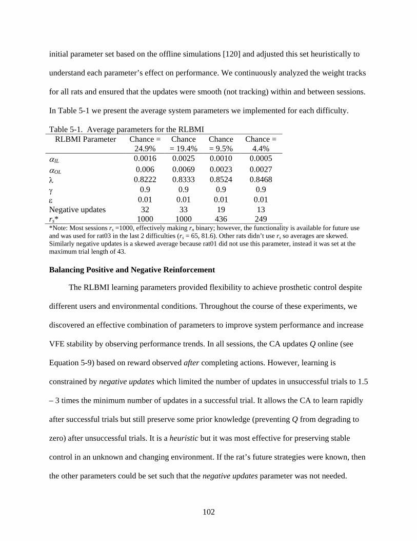
102

initial parameter set based on the offline simulations [120] and adjusted this set heuristically to

understand each parameter’s effect on performance. We continuously analyzed the weight tracks

for all rats and ensured that the updates were smooth (not tracking) within and between sessions.

In Table 5-1 we present the average system parameters we implemented for each difficulty.

Table 5-1. Average parameters for the RLBMI RLBMI Parameter Chance =

24.9% Chance = 19.4%

Chance = 9.5%

Chance = 4.4%

αIL 0.0016 0.0025 0.0010 0.0005 αOL 0.006 0.0069 0.0023 0.0027 λ 0.8222 0.8333 0.8524 0.8468 γ 0.9 0.9 0.9 0.9 ε 0.01 0.01 0.01 0.01 Negative updates 32 33 19 13 rs* 1000 1000 436 249 *Note: Most sessions rs =1000, effectively making rn binary; however, the functionality is available for future use and was used for rat03 in the last 2 difficulties (rs = 65, 81.6). Other rats didn’t use rs so averages are skewed. Similarly negative updates is a skewed average because rat01 did not use this parameter, instead it was set at the maximum trial length of 43. Balancing Positive and Negative Reinforcement

The RLBMI learning parameters provided flexibility to achieve prosthetic control despite

different users and environmental conditions. Throughout the course of these experiments, we

discovered an effective combination of parameters to improve system performance and increase

VFE stability by observing performance trends. In all sessions, the CA updates Q online (see

Equation 5-9) based on reward observed after completing actions. However, learning is

constrained by negative updates which limited the number of updates in unsuccessful trials to 1.5

– 3 times the minimum number of updates in a successful trial. It allows the CA to learn rapidly

after successful trials but still preserve some prior knowledge (preventing Q from degrading to

zero) after unsuccessful trials. It is a heuristic but it was most effective for preserving stable

control in an unknown and changing environment. If the rat’s future strategies were known, then

the other parameters could be set such that the negative updates parameter was not needed.

103

VFE Network Learning Rates

The VFE network learning rates were also very effective parameters for controlling

adaptation of the CA. The input layer learning rate aIL controlled changes in the neuronal data

projection and state segmentation. It was important to preserve the state; increasing aIL could

entirely destabilized the RLBMI. However, aIL did allow the state to adapt to changing neuronal

signal (e.g. neuron loss) over multiple sessions. The output layer learning rate aOL had more

effect on the actual value Qk of each possible action. It was most effective for the output layer to

learn at least five times faster than the input layer and to reduce both learning rates by 20%

between each session. This suggests that the RLBMI system is more capable of adjusting values

for existing state-action pairs, than rapidly re-segmenting the state space and evaluating new

state-action pairs; this agrees with intuition.

Reinforcement Learning Parameters

The RL specific parameters had more influence on CA learning within a session than

between sessions. The λ parameter (see Equation 5-4) partially controls the balance in the weight

update; it was initially set based on the minimum trial length and adjusted based on performance.

The discount factor γ controls the reward horizon but was kept constant throughout sessions to

preserve prior VFE mappings as task difficulty increased. It is probable that γ should have been

adjusted to help the RLBMI transition to more difficult task. The optimal VFE output will

change as task difficulty increases (if γ is constant) because it approximates return (see Equation

2-1). It is likely that we should have attempted to change γ in the fashion we changed λ and kept

λ constant as λ relates to averaging different return estimates. Exploration ε was useful for a

naïve CA and rat to earn reward. However, ε slows value function adaptation (see Equation 5-7);

hence, ε is kept under 1% in developed VFE networks. The rs term (see Equation 3-1) was

104

helpful in one rat; however, it is a sensitive parameter that needs future investigation. Like

negative updates, rs is a sensible hack that is grounded in RL concepts but would not be needed

if we knew the rat’s strategies a priori and could set the other RL parameters more appropriately.

Session to Session RLBMI Adaptation

After giving the rats a random VFE in the initial control session, we were able to rapidly

train a useful VFE given their neural modulations. The rats then performed 80-200 brain control

trials using this RLBMI each day (each session). The rat is not told explicitly that it is in brain

control since all four levers are extended for each trial. The rats tended to remain stationary in

the center of the cage directly in front of the water center, eyes facing the robot workspace.

However, the rat continued to generate different neuronal modulations during control; this is

thoroughly examined in Chapter 6. Essential to the success of this brain-control task is the

coupling of the motivation and actions (neuronal modulations) of the rat with the CA’s action

selection (robot movements). While the rat is learning which neuronal modulations result in

water rewards, the CA must adapt to more effectively respond to the rat’s brain.

Multiple sessions were used to show the ability to use past experience and adapt to novel

situations in a dynamically changing environment. The complete brain control paradigm

provides a mechanism to directly control task difficulty with dthres in Equation 3-1. Increasing

task difficulty between sessions demonstrates the RLBMI’s ability to adapt to changing

environmental dynamics. In brain control dthres is initially set low to increase the probability of

trial success; this keeps the rat engaged and facilitates RLBMI co-adaption to the early portion of

the task. After a rat demonstrates greater than 60% accuracy (brain control inclusion criterion)

for both targets in a session, task complexity was increased in the next session.

The weights were preserved between successful sessions, i.e. the final VFE weights were

used as initial weights for the next session. If the rat exceeded the brain control inclusion

105

criterion and/or the VFE network was stable, the session was considered a success. However

some sessions were failures (e.g. VFE destabilization, hardware failures) and their final VFE

weights were discarded with the next session being initialized using the last successful session.

Some rats had a significant decrease (sometime absence of) in specific neuronal unit’s

firing in later sessions. The unit remained in the neural state although the firing rate may be zero.

In other cases a new unit was detected in later session and replaced a missing unit in the state.

Rat and VFE network co-adaption faciliated the RLBMI to accommodate these state changes.

Performance of RLBMI Users

The performance and usefulness of the RLBMI was evaluated only during brain control

tasks9. During brain control, all rats typically remained motionless near the reward center,

faced the robot workspace, and relied on using neural activation to interact with the CA. For

goal-based BMI applications, the speed and accuracy of completing the task are two primary

metrics that demonstrate the functionality of the interface. In this experimental paradigm, we

quantify the percentage of trials in which the rat successfully navigated the 3-D workspace with

the robotic arm to achieve a reward (PR) and compare with random walks of the robot. In

addition to quantifying the successful trials, we measure the time that it takes to reach a target

(TT). We expect that coordinated control will yield PR several times greater than chance level

and use more direct paths; hence faster TT.

For each of the three10 rats involved in the study, co-adaptation of a single RLBMI model

occurred over multiple sessions (1 session per day, 2.1 +/- 1.2 sessions per dthres, and 141.6 +/-

41.3 trials per session). After each rat met the performance inclusion criterion (PR = 60%), the 9 All results are from continuous co-adaptation over multiple sessions with no offline VFE retraining or adjustment.

10 Four rats were prepared for this study; however, one rat dislodged his electrodes before starting the brain control experiments and had to be sacrificed. We felt three rats were sufficient because of the number of total sessions (25) and total number of neurons (62). Those numbers are in line with prior rat BMI publications.

106

reaching task complexity was increased (i.e. the number of successive actions necessary to earn

reward) between sessions to shape the rat toward the most complex task. The PR and TT metrics

were calculated in brain control for each dthres and compared to chance performance as estimated

in the next subsection. The chance PR provides a metric of task difficulty in all analysis.

Defining Chance

Chance PR is calculated using five sets of 10,000 simulated brain control trials using

random action selection (random walks in the robot workspace). The PR from each set of trials is

then used to calculate the average and standard deviation. Chance TT is calculated from the

concatenation of the 5 sets of random trials. Although, learning algorithms such as RLBMI can

learn to outperform random walks (see Chapter 2), prominent prior BMI literature has used

similar random walk models to define chance [59, 62, 68, 72, 98, 147]. The data used to

calculate chance PR and TT is also used in 2-sample Kolmogorov-Smirnov (K-S) (95%

significance) tests for statistical comparisons with each rat’s performance.

Additionally, we repeated the surrogate neural data tests from our prior work [120] to

determine if the CA could learn a solution regardless of information in the state, e.g. leaning

from the rewards alone. Rat neuronal firing rates were randomized temporally and spatially and

then processed through the γ structure to create a surrogate state. A surrogate VFE network was

created using the average RLBMI parameters reported in Table 5-1 and offline batch training.

The network is trained for the same average number of trials and sessions at each difficulty. The

performance of both the chance (random walk) and surrogates are reported with the rat’s results.

Accuracy: The Percentage of Trials Earning Reward (PR)

Accuracy of each RLBMI is presented in Figure 5-5: a-c which shows each rat’s left and

right target PR averaged over trials for each difficulty. While co-adapting with the CA, each rat

achieved control that was significantly better (2 sample K-S test, α = 0.05) than chance for all

107

task complexities. RLBMI average (over difficulties and targets) PR was 68%, 74%, and 73%

for rats 1, 2, and 3 respectively (average chance PR is 14.5%). Additionally, the individual PR

curves indicate that the co-adaptation is enabling the RLBMI to retain or improve performance in

increasingly complex environments. This may reflect the role of co-adaptation in the RLBMI.

In Figure 5-5d, both the surrogate and chance PR are shown. The surrogate network did

learn to guess one target (right side) for all trials with an average PR of 47%. Without causal

neuromodulation (without information in the state) from the rat only one action selection strategy

(independent of the state) was being used by the CA instead of generalizing to the overall task.

This is analogous to always guessing heads in a series of coin flips after seeing that one flip was

heads, the guesser should be correct in approximately 50% of the trials. This is the extent that the

CA can learn from rewards without an informative state – the CA will guess whichever target

has randomly earned a reward and ignore the other targets yielding overall success of 1/targets.

Figure 5-5. Percentage of successful trials. (a-c) The left and right PR (top) and the number of

sessions performed at each difficulty (bottom) for rat01, rat02, and rat03 respectively. (d) PR for the surrogate neural data. Error-bars are the 95% confidence intervals.

108

We also present the 95% confidence intervals as error bars (also shown on chance curves

but are difficult to see given the y-axis scale). The confidence intervals changed between the 2nd

step to the final step by -16%, +26%, and -1% for each rat as task difficulty increased. However,

the number of trials in later sessions masks increases in standard deviation of 124%, 389%, and

364%. The PR variance with increasing task difficulty is partially due to lower PR in sessions

where the rat and CA to co-adapt to a novel environment. At the 2nd difficulty level, rats were

within 9% of the inclusion criteria for all sessions. However, all rats had at least one session 20-

35% below the inclusion criteria as the rat and CA learned to solve the final difficulty level.

Speed: The Time to Reach a Target (TT)

Figure 5-6 shows each rat’s left and right TT averaged over trials of the same difficulty vs.

task difficulty (the number of sessions is identical to Figure 5-5). The chance TT is also plotted

for reference (the surrogate TT was not used because that network was unable to complete both

tasks). All three rats achieved significantly faster (2 sample K-S test, α = 0.05) trial completion

than chance for all task difficulties. RLBMI average (over difficulties and targets) TT was 1.3 s,

1.1 s, and 1.1 s for rats 1, 2, and 3 respectively (average chance TT is 2.7 s). The optimal TT was

computed by the time needed to move directly to each target along the shortest path. Each

increase in task difficulty increased the theoretical minimum TT because the targets are farther

away. Instances where the TT curve has a less negative slope than the optimal TT suggest that co-

adaptation of the RLBMI can improve prosthetic control.

The actions used by the RLBMI also affect both PR and TT for each target. The rats

exhibited different left and right trial PR despite the trial difficulty being the same by design (all

actions are the same vector length and targets are equidistant from the initial robot position).

However, each CA co-adapted over time with the user to only use a subset of the possible actions

109

and users may have different strategies to reach each target. This has the net effect of

unbalancing the task difficulty for left and right targets. The set of actions most commonly used

by the RLBMI also affect TT for each target. For example, rat02 and rat03’s left TT were longer

than the right TT indicating they used less direct paths to the left target.

Figure 5-6. Robot time-to-target vs. task difficulty. Error-bars are the 95% confidence intervals

Action Selection Across Sessions

The distribution of actions selected for each session illustrates the RLBMI action selection

strategy. The agent seeks to maximize Rt and could accomplish this by minimizing TT using only

2 tri-directional direct actions to move the robot directly to the target. Figure 5-7a shows the

distribution of the most used actions in rat02’s successful left trials (representative of all rats).

The RLBMI selected robot actions directly towards (R-FWD-UP) the right target 50% of the

time. The RLBMI selected corrective actions towards the left (correct) target for 40% of the

time. However, Figure 5-7b shows that a single, direct action is selected in 90% of successful

right trials. Additionally, the RLBMI initially used a larger subset of five actions but over time

the subset is reduced to three. This shows that training may still be improved – the rat strategy

may be sub-optimal due to experimental conditions (e.g. visual feedback).

110

Figure 5-7. RLBMI Action Selection for rat02. (a) Left trials (b) Right trials. Action selection is

representative of all rats: one action for a target and mixed actions for the other target.

Relationship of action selection to performance

The differences in action selection illustrated in Figure 5-7 explain the TT difference in

Figure 5-6b: right trials are almost three times faster because the robot moves directly to the

target in successful right trials. Also the change in the left TT in Figure 5-6b after the 3rd session

can be explained by the changing strategy observed in Figure 5-7a. After the 3rd session the

RLBMI becomes less likely to use a combination of actions that maneuver the robot towards the

left target; instead the combination of actions includes actions away from the target and

corrective actions. This creates less direct paths; it follows that TT increases.

Rationale for action set reduction over time

An optimistic explanation is that all RLBMI systems adapted to an action subset which

facilitated visual feedback to correct robot trajectories. If the action set only included two direct

actions, the rat could minimize TT moving directly to both targets. In the event the RLBMI

initially used the incorrect direct action, the rat would receive visual feedback of a control error;

however, even if the rat modulated neuronal firing to select the other direct action, it would be

unable to successfully maneuver the robot to the correct target. Instead the robot would move

111

towards the lever but reach a workspace boundary (wall) condition and stop short of reaching the

correct target – failing to earn a reward. Changing the safety constraints of the robot workspace

may allow both optimal action sets and the use of visual feedback.

Alternatively, it is possible that the rat and CA was forced to co-adapt to a smaller action

set because of the VFE network training methods employed. Since there was no mechanism to

predict the future neural states, the CA could only learn from experience (actions selected) and

not prediction. But this creates a catch-22: the CA cannot update new actions until trying them

but the CA will not try new actions until they are updated. The exception to this rule is the

exploration aspect of Q(λ) learning, but ε is set to 1% which means that any particular action had

a (1/26)% chance of being used and then updated.

We initially thought the soft max policy would partially solve this problem because it

explores to the next-best action – increasing the chance of updating other potentially important

actions but ignoring actions with likely low importance [103]. This can speed learning and

increase accuracy even though there is no guarantee that the next-best actions are in the general

direction of the target. Soft-max was a component of the offline simulations because of its

potential advantages. However, soft-max could not be implemented because the cost of

theoretical superiority was experimental instability. Stability vs. performance was a common

tradeoff in the RLBMI and will be addressed in Chapter 7.

Conclusions

This chapter started with a set of unanswered questions that was preventing RLBMI

implementation. These challenges were overcome by combining insight from offline simulations,

RL literature, and actual experience with the online BMI. The VFE was achieved with a MLP

with a non-linear hidden layer but linear output PEs. The VFE network was trained using an

112

implementation of Watkin’s Q(λ) Learning because of potential learning advantages over similar

techniques, e.g. SARSA or Q-Learning [103]. Rather than reinvent RL, we took advantage of

available computing resources, efficient scheduling, and batch training to over come the known

slow RL learning. With the experience gained here and the computational power of the Cyber-

Workstation, the next generation of RLBMI designers could tap the potential of more advanced

VFE networks and RL training methods. Performance improvements in this coupled RLBMI

architecture potentially will create positive feedback, CA improvement encourages rat

improvement and rat improvement encourages further CA improvement.

The large parameter set was problematic and we obviously cannot claim to have explored

all possible combination. However, through experience, RL, and ANN concepts we found an

effective set to facilitate user control, co-adaptation over time, and robot control stability. These

parameters provide rich opportunities to distribute the adaptation and control burden and this

aspect will be further explored in future research tracks dedicated solely to that concept.

To demonstrate the utility of co-adaptation we ran the RLBMI experiments for multiple

sessions where the task difficulty changes. This is both a way to show adaptation to

environmental change and shaping through a BMI to facilitate complex tasks/ movements.

Previously, Schwartz et al. conditioned monkeys to control a prosthetic arm with a form of

shaping in a reach and grasp task [10]. The paradigm required the monkeys complete the reach to

the food target; then the robot automatically completed the grasp portion [148]. Years later (new

research) they showed this shaping was finally able to help the monkeys further developed their

control abilities and could complete the grasps/ releases with brain control [149].

Shaping is potentially beneficial to both the rat and CA. Both parties learn portions of the

task and may build on prior learning to master the complete task. The rats were all able to use the

113

RLBMI over multiple days without retraining or a desired signal in a changing environment.

Additionally the rat’s neuro-modulations were changing over this time (see Chapter 6). However,

it is not possible to conclude whether shaping was helpful (or occurred) for the rats without

control subjects. It is unknown if the rats would generally perform at the brain control inclusion

criteria (60% PR) in the most complex task unless they were shaped towards it. Refining the

experimental design and providing more controls should reveal any advantages of shaping.

Finally we needed to quantify the performance of the closed loop RLBMI. The RLBMI

exploited spatiotemporal structure in the firing of 16-29 MI neurons; this formed the state which

reflected the rat’s goals and perception of the workspace. The CA learned to select sequences of

prosthetic actions to complete the tasks (earn reward) which suggests sequences of states were

distinct for different tasks. In the next chapter we investigate the neurophysiology and VFE

network descriptors at a low level of abstraction. In this chapter we focused on overall robot

control at a high level of abstraction from an engineering perspective. Specifically, we quantified

the ability of the RLBMI (both rat and CA) to acquire each target over multiple trials with PR.

Additionally, we quantified the speed which the RLBMI would complete successful trials with

TT. Although classic psychometric curves [119] predict a steady performance decrease with

increased difficulty, each rat exhibits at least one instance of increased PR (or decreased TT

relative to the optimal TT) with task difficulty (see Figure 5-5: a-c top). This may reflect the role

of co-adaptation in the RLBMI. Action selection strategies can also affect both the PR and TT;

Chapter 6 also expands on this. The composition of the limited action set suggests that the rats

did not fully use all the actions that were available in the brain control task. This likely indicates

a combination of: rats ignoring inefficient actions, rats selecting an action set to enable visual

114

feedback, the VFE training was sub-optimal, or insufficient neuro-modulations to trigger all

actions (see Chapter 6). Chapter 7 will propose a new method to overcome this issue.

Although theoretically closing the loop should dramatically improve RLBMI performance,

it is difficult to contrast the online results with the offline simulations. The main reason for this is

the vastly increased complexity of the online tests and current inability to batch train the

networks quickly enough to replicate the offline test conditions (rat remains in cage). However,

the differences in action subsets may be revealing. The offline RLBMI simulations used the two

direct-to-target actions exclusively. The online RLBMI used one direct-to-target action and one

to three other indirect-to-other-target actions. This again supports our hypothesis (based on

training) that the rats were using visual feedback in the online experiments.

115

CHAPTER 6 CO-EVOLUTION OF RLBMI CONTROL

Introduction

Validation of the new BMI control architecture developed in this dissertation was first

achieved by quantifying task performance metrics: target acquisition and task speed. The

previous chapter provided the necessary evidence that three rats could complete reaching tasks

through the RLBMI despite a changing environment over multiple days. The task metrics

demonstrate the feasibility of the architecture but are performance-based and not appropriate for

understanding the mechanisms of prosthetic control.

The rat and Computer Agent (CA) are both intelligent systems in the RLBMI and it was

unclear how the adaptive properties and activity of these systems contributed to control. For

example, the rat can adjust the fine timing relationships between neuronal activations and the CA

can adapt the value of each prosthetic action. Here, we investigate four specific areas to

understand the co-evolution of control:

• Prosthetic action representation in rat neural modulations • Mechanisms of CA RLBMI control • Mechanisms of rat RLBMI control • Co-evolution of control

The first two areas consider each intelligent system independently. This separation is not

imposed to ignore the rat-CA coupling but rather to provide the necessary concepts to understand

how both can act synergistically. Statistical analysis reveals significantly different representation

for robot actions within the rat’s neural modulations. This representation is quantified through

the established method of directional tuning [52, 54]. Directional tuning has been applied to both

open and closed-loop BMI [52, 54, 59, 61, 99, 150] to specify what neurons are most correlated

with (tuning direction) and how strong that correlation is (tuning depth). This analysis is shows

116

that a set of prosthetic movements could be encoded in the rat’s motor cortex. However, it uses

correlation to show that the representation exists and does not show how the neural modulations

drive the RLBMI networks.

Understanding network operation requires understanding how the CA exploits the different

neural modulations to assign action values. The CA adapts the value function estimator (VFE)

network [86] based on the fundamental concept of return (see Equation 2-1). The VFE output

correlates with the return after adaptation. However, there are some areas where it is clear that

the training mechanisms and/ or state signal could be improved.

Evidence of synergistic activity can then be extracted from the functional connections that

couple the rat and CA. This analysis reveals a subset of efficient neurons and network

descriptors. After distilling the contributions and interactions of the rat and CA, we illustrate how

RLBMI control evolves over time. Implications of these results for the general BMI community

(users and designers) are provided in the conclusion.

Action Representation in Neural Modulations

All rats in this study exhibited behavior which suggested they were engaged in the

prosthetic control task [86]. Specifically, they typically remained motionless near the reward

center, faced the robot workspace, and maneuvered the robot based on visual cues. However, this

does not reveal which workspace variable (e.g. robot position, LED cues, rewards, robot

movement) the rat is attentive to.

Since the rat training (see Chapter 3) shapes the rat to attend to the robot movements,

directional tuning is calculated relative to these movements (RLBMI actions) [150]. This tuning

reveals an action representation in the neural modulations for all rats. This action representation

contrasts with tuning relative to other variables (i.e. robot position) which did not reveal

117

obviously tuning [150]. The approach of tuning to robot actions is similar, albeit in an artificial

prosthetic, to other groups which have shown tuning relative to the user’s arm velocity [52, 54].

Conditional Tuning to Actions

Specifically, we define a conditional tuning θ in Equation 6-1 where n is the neuron index,

k is the index of the robot action, and FRn is the firing rate of the nth neuron. Traditional tuning is

different than conditional tuning because traditional tuning assumes a single preferred direction

for each neuron based on the most excitatory response [59, 61, 99, 150]. That restriction is

logical when interfacing with the user’s motor system (e.g. able-bodied BMI users). However,

we are not constrained by the rat’s musculoskeletal system and allow for either inhibitory or

excitatory neural representation of each action. Thus, there is a conditional tuning for each action

instead of restricting each neuron to a single preferred direction. Additionally, to show illustrate

differences, the conditional tuning is normalized by the mean FR to create a depth for each

action in Equation 6-2. This is another departure from traditional tuning which assigns one

tuning depth based on FR in the preferred direction.

( )kactionFRmean nkn == |,θ (6-1)

( )actionsFRmeandepth nknkn ∀−= ,, θ (6-2) Illustrating Conditional Tuning for an Action Subset in a Single Session

While it is possible to compute conditional tuning to any selected action, the rats all used a

subset of three actions over all sessions. The rationale for this action selection was discussed in

Chapter 5. Briefly, we hypothesized that the action set results from a combination of the rat

selecting actions which enable corrections via visual feedback, the low penalties not forcing

optimal control paths, and the VFE training mechanism only updating small action sets.

Conditional tuning for the three most used actions was calculated in the session when the

rat reached the inclusion criteria for the 2nd difficulty level. At this session, each rat had

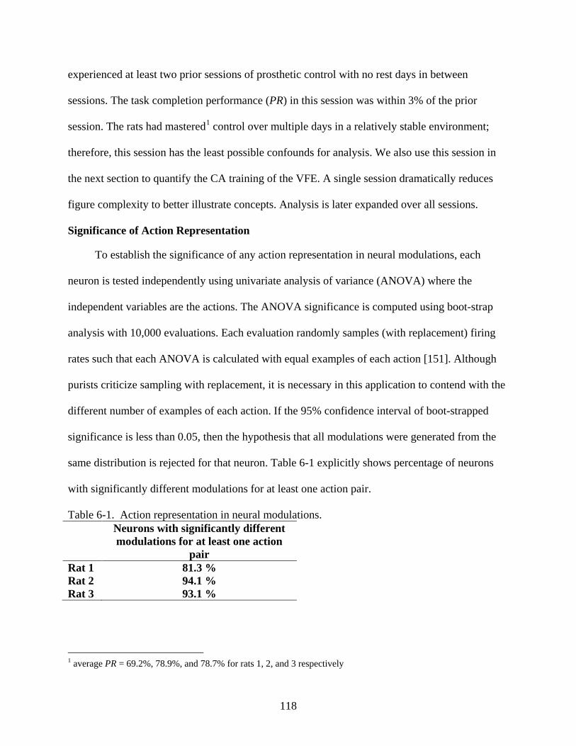
118

experienced at least two prior sessions of prosthetic control with no rest days in between

sessions. The task completion performance (PR) in this session was within 3% of the prior

session. The rats had mastered1 control over multiple days in a relatively stable environment;

therefore, this session has the least possible confounds for analysis. We also use this session in

the next section to quantify the CA training of the VFE. A single session dramatically reduces

figure complexity to better illustrate concepts. Analysis is later expanded over all sessions.

Significance of Action Representation

To establish the significance of any action representation in neural modulations, each

neuron is tested independently using univariate analysis of variance (ANOVA) where the

independent variables are the actions. The ANOVA significance is computed using boot-strap

analysis with 10,000 evaluations. Each evaluation randomly samples (with replacement) firing

rates such that each ANOVA is calculated with equal examples of each action [151]. Although

purists criticize sampling with replacement, it is necessary in this application to contend with the

different number of examples of each action. If the 95% confidence interval of boot-strapped

significance is less than 0.05, then the hypothesis that all modulations were generated from the

same distribution is rejected for that neuron. Table 6-1 explicitly shows percentage of neurons

with significantly different modulations for at least one action pair.

Table 6-1. Action representation in neural modulations. Neurons with significantly different

modulations for at least one action pair

Rat 1 81.3 % Rat 2 94.1 % Rat 3 93.1 %

1 average PR = 69.2%, 78.9%, and 78.7% for rats 1, 2, and 3 respectively

119

This analysis is bottom-up by design – it considers at correlations between robot actions

and neuronal modulations and does not incorporate the causality between neural modulations and

action selections. (That top-down analysis is reserved for the third section of the chapter.)

Instead, this analysis is performed because physiology suggests that the rat’s neurons should

modulate with some relationship to muscle activation [28, 152]. However, as in [153] we found

that the rats could also modulate with respect to an external prosthetic.

Averaging across all three rats, 90% of recorded neurons had significantly different

modulations relative to robot actions. This is result is higher, albeit not directly comparable, with

another group which found 66% (averaged of three monkeys) of recorded neurons had

significantly (via ANOVA) different modulations for at least one pair of tuning directions [154].

It is important to note that we have fewer actions which may inflate the number of significantly

tuned neurons. (This inflation occurs in the rat data because there are more samples for each

action; hence, lower variance in the distributions.) For reference, I also performed a surrogate

analysis where the neural data was preserved but the corresponding action labels were

randomized and found an average of 1.6% of neurons with significantly different modulations.

Again, this is a correlation analysis so shuffling the outputs is equivalent to shuffling the inputs.

For the 90% of neurons where the ANOVA hypothesis was rejected, post-hoc tests were

conducted to determine which action-pairs were significantly different (ANOVA alone does not

provide this information). All post-hoc tests were tested at 0.05/3 using the Bonferroni correction

to control for errors due to the number (three) of comparisons [155, 156]. The results of all pair-

wise significance tests are given in Table 6-2. For two of the rats significance still cannot be

calculated for all action pairs due to one action being selected less than 5% of the time. Although

bootstrapping is can overcome some sample differences, the number of samples was affecting

120

the tests. For example, if these actions were not excluded then the ANOVA analysis would show

that 75% of the neurons were tuned, a reduction of 15% from the values reported in Table 6-1.

Table 6-2. Post-hoc significance tests between actions Rat 1 Neurons* Rat 2 Neurons* Rat 3 Neurons*

state BR ≠ state FRU

** state BL ≠ state F

98.5 % state L ≠ state FRU

99.2 %

state BR ≠ state FLU

95.7 % state BL ≠ state FRU

65.1% state L ≠ state FLU

***

state FRU ≠ state FLU

** state F ≠ state FRU

86.3 % state FRU ≠ state FLU

***

* Post-hoc tests of significant differences are shown only for neurons with significant (p < 0.05) ANOVA (see Table 6-1). Confirmed post-hoc tests represent the percentage of 10,000 tests which showed significant differences (p < 0.05/number_of_comparisons) between the pair of actions. ** Action FRU was selected < 4% of the time. This difference in sample size could not be overcome with replacement. Therefore it was excluded from the analysis for this session *** Action FLU was selected < 1% of the time. This difference in sample size could not be overcome with replacement. Therefore it was excluded from the analysis for this session

BR FRU FLU-505

10

Rat

1D

epth

[Hz]

Left Motor Cortex

BR FRU FLU-505

10Right Motor Cortex

BL F FRU-20-10

010

Rat

2D

epth

[H

z]

BL F FRU-20-10

010

L FRU FLU

0

1020

Rat

3D

epth

[H

z]

ActionL FRU FLU

0

1020

Action Figure 6-1. Neural tuning to RLBMI actions. The recorded neurons with the maximal depth (for

any action) from each motor cortex (columns) are presented for each rat (rows). The action pairs connected with a line and * contain significantly different neural modulations. Tuning is calculated for the session where the rats reached the inclusion criteria for the 2nd difficulty level.

Figure 6-1 shows the neurons with the maximal depth (Equation 6-2) for any action from

each hemisphere of motor cortex. Actions pairs found significantly different in at least 95% of

the boot-sampling post-hoc tests (i.e. at least 9,500 of the 10,000 boot-strap tests were significant

121

at p = 0.05/3) are also labeled with a *. Within the ensemble of recorded neurons for each rat,

significantly tuned neurons appeared to use a similar modulation strategy for each action. If

neurons A and B were both significantly tuned to action C then both neurons would increase

(decrease) FR for action C, i.e. both neurons have positive (negative) tuning depth for action C.

There were no counter-examples in the three rats.

This representation regardless of hemisphere is surprising because our prior neural analysis

show different neural modulation patterns (through peri-event histograms) in rats making

stereotypical presses in task similar to the animal training (see Figure 3-5, more details available

in [104]). There were different modulation patterns in the left and right cortex depending on

which arm the rat was using to press the lever. Equivalently, there were different patterns for

each target/cue because the rat could not complete the task without a stereotypical press. Here we

do not find target/cue-related modulations; instead they are related to actions. Additionally, the

analysis supports our claim that the rats are not making limb movements to control the

prosthetic. If rats were making these movements, we would expect different modulation patterns

between hemispheres. Again, we do not see these differences in the rats.

Figure 6-1 also shows that the recorded neurons showed excitation for certain actions (e.g.

action F, rat 2) and inhibition for other actions (e.g. action FRU, rat 3). Other groups have also

shown that neurons can use inhibitory and excitatory modulation to achieve prosthetic control

[153]. The analysis in this sub-section established that the rats actively modulated neurons based

on RLBMI actions for one session. The next sub-section expands the analysis over all sessions.

Evolution of Action Representation

The ANOVA significance tests from the prior section are repeated over all sessions for the

same actions. Figure 6-2 shows the percentage of the neural ensemble that significantly

modulates for at least one action pair (as in Table 6-1). Figure 6-3 shows the post-hoc tests to

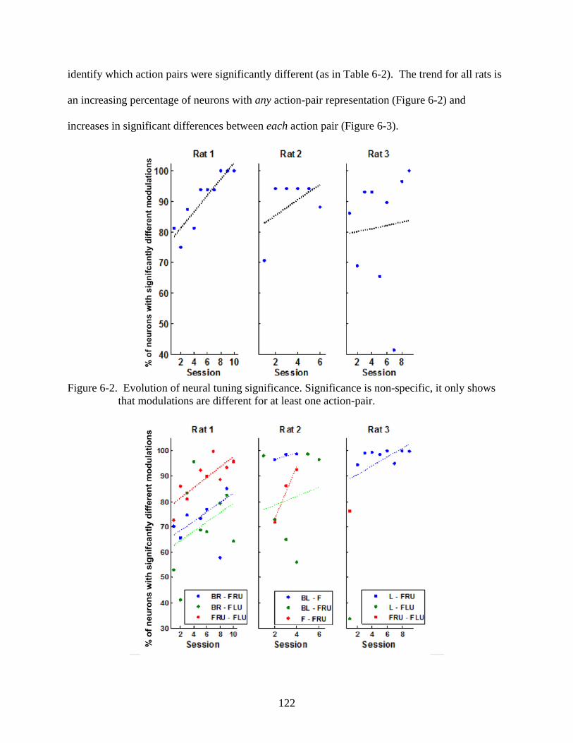
122

identify which action pairs were significantly different (as in Table 6-2). The trend for all rats is

an increasing percentage of neurons with any action-pair representation (Figure 6-2) and

increases in significant differences between each action pair (Figure 6-3).

Figure 6-2. Evolution of neural tuning significance. Significance is non-specific, it only shows

that modulations are different for at least one action-pair.

123

Figure 6-3. Evolution of neural tuning significance between each action-pair. Significance is determined with post-hoc tests on neurons identified in Figure 6-2. To be significant at least 9,500 of the 10,000 boot-strap tests were significant at p = 0.05/3.

It is important to also note that Figure 6-3 that the averages are only among those neurons

identified as having significant differences in FR for at least one action pair. Figure 6-2

illustrated that all rats had relatively less neurons with significant differences in the initial

sessions. If all neurons (significant or not) were included in Figure 6-3, then the early sessions

would be further decreased and the slopes over sessions would increase. If an action was selected

less than 10% of the time (see Figure 6-11), then there are no data-points for comparisons with

that action. For all rats, the action pair that is most often used2 has data-points for all sessions.

Figure 6-1 showed (along with Tables 6-1 and 6-2) that there was a statistically significant

representation of the robot actions in the rat’s neuronal modulations. Additionally, Figures 6-2

and 6-3 showed that this representation became present in a greater percentage of neurons over

time as the rats continued to control the robot. However, we still cannot address how these neural

modulations contribute to action selection. To reach that level of analysis, we need to first

understand and quantify the CA control mechanisms.

Mechanism of Computer Agent RLBMI Control

Prior chapters (2 & 5) have established the procedure for the CA to control the prosthetic

arm. Briefly, the VFE network estimates the value of all 27 possible actions given the current

neural state. The CA follows a policy (ε-greedy) which typically exploits prior learning, i.e. it

selects the action with the maximum value. The robot arm completes this action and then the CA

observes a reward from the environment. The CA uses the observed reward to train the VFE to

approximate the expected return [103] for taking a specific action given the neural state [103].

2Most commonly used actions over all sessions: Rat 1: BR vs. FLU. Rat 2: BL vs. FRU. Rat 3: L vs. FRU

124

For convenience the return (R) at time t is reprinted in Equation 6-3 where γ is a discounting

factor, T is the remaining trial length, and rn is the reward at time n. The reward is 1 after a trial

is successful and -0.01 all other times. Figure 6-4 shows Rt for both successful and failed trials.

Even in successful trials, it is possible to have a negative R if the trial will not be completed

within 25 steps. This time is a function of γ, higher γ will prevent negative R in successful trials.

∑

+=

+−=T

tnn

tnt rR

1

1γ (6-3)

0510152025303540

0

0.2

0.4

0.6

0.8

1

Steps to Trial Completion

Ret

urn

Successful TrialsFailed Trials

Figure 6-4. Actual return for successful and failed trials. Return decreases exponentially as more

steps are required to complete the trial. Return is calculated based on γ =0.8333, the same value used for all rats in this session.

Estimated Winning Value vs. Actual Return

The CA is selecting the action which should maximize R through selecting the maximum

value. However, the CA updates the VFE based on the R which actions have earned. Thus the

CA adapts the VFE toward appropriate values through interaction with the environment and can

adapt to maintain control if the environment changes. This adaptive capability should cause the

VFE output to correspond with actual R [86, 103]. The average state-action value function

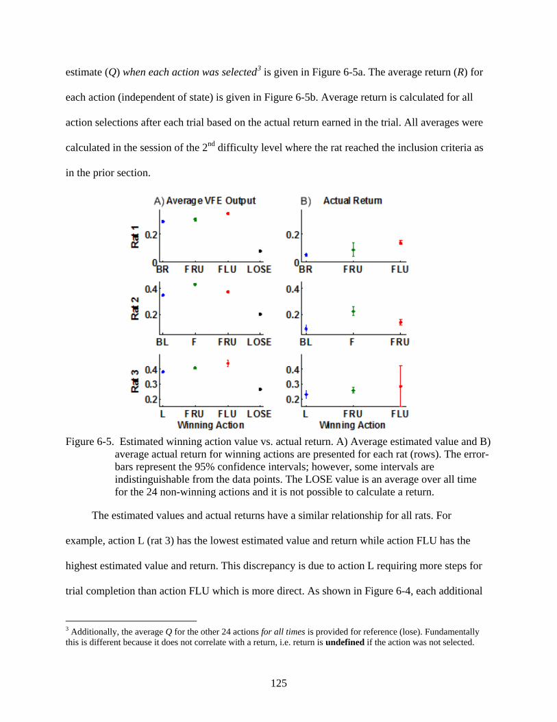
125

estimate (Q) when each action was selected3 is given in Figure 6-5a. The average return (R) for

each action (independent of state) is given in Figure 6-5b. Average return is calculated for all

action selections after each trial based on the actual return earned in the trial. All averages were

calculated in the session of the 2nd difficulty level where the rat reached the inclusion criteria as

in the prior section.

Figure 6-5. Estimated winning action value vs. actual return. A) Average estimated value and B)

average actual return for winning actions are presented for each rat (rows). The error-bars represent the 95% confidence intervals; however, some intervals are indistinguishable from the data points. The LOSE value is an average over all time for the 24 non-winning actions and it is not possible to calculate a return.

The estimated values and actual returns have a similar relationship for all rats. For

example, action L (rat 3) has the lowest estimated value and return while action FLU has the

highest estimated value and return. This discrepancy is due to action L requiring more steps for

trial completion than action FLU which is more direct. As shown in Figure 6-4, each additional

3 Additionally, the average Q for the other 24 actions for all times is provided for reference (lose). Fundamentally this is different because it does not correlate with a return, i.e. return is undefined if the action was not selected.

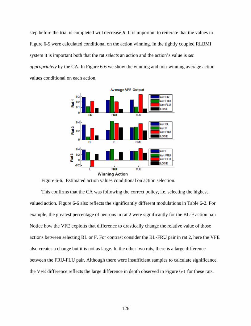
126

step before the trial is completed will decrease R. It is important to reiterate that the values in

Figure 6-5 were calculated conditional on the action winning. In the tightly coupled RLBMI

system it is important both that the rat selects an action and the action’s value is set

appropriately by the CA. In Figure 6-6 we show the winning and non-winning average action

values conditional on each action.

Figure 6-6. Estimated action values conditional on action selection.

This confirms that the CA was following the correct policy, i.e. selecting the highest

valued action. Figure 6-6 also reflects the significantly different modulations in Table 6-2. For

example, the greatest percentage of neurons in rat 2 were significantly for the BL-F action pair

Notice how the VFE exploits that difference to drastically change the relative value of those

actions between selecting BL or F. For contrast consider the BL-FRU pair in rat 2, here the VFE

also creates a change but it is not as large. In the other two rats, there is a large difference

between the FRU-FLU pair. Although there were insufficient samples to calculate significance,

the VFE difference reflects the large difference in depth observed in Figure 6-1 for these rats.

127

Observed Differences between VFE Outputs and Return

The CA trained the VFE based on the principles [103] of return. However, Figure 6-5

showed that the VFE performance does not exactly approximate return, instead Q is only

correlated with R. There are bias and variance errors in VFE performance so it is reasonable to

question the efficiency of the CA training. Here we provide explanation of each error and

potential methods to overcome them in the future.

Bias in the VFE network

The returns for winning actions are similar to the estimated values of losing actions. The

VFE should have adapted to accurately predict the winning action returns, lowering those

action’s values. The CA would then begin selecting one of the higher-valued actions which had

previously lost. That behavior follows RL principles exactly, but could be catastrophic from a

control perspective. Since losing actions have not (or rarely) generated a return; their estimated

value (and relationship to neural states) is undefined. The VFE network training and/ or action

selection policy should be refined to prevent this problematic situation of undefined values. In

the absence of this improvement, the bias in the VFE output may be beneficial ‘error’ for

maintaining stable control. This bias may also have been preserved externally via the VFE

learning rate; the learning rates are addressed in the last session.

Variance in the VFE network

The VFE output does not accurately reflect the return variance which is an order of

magnitude larger than the VFE variance (see Figure 6-5). The first section established that neural

modulations are different based on actions, but it did not address if rats significantly modulated

firing based on the return (within actions). The ANOVA tests for each neuron are repeated with

128

actual return4 as the independent variable. Averaging over all rats, only 5% of neurons were

significantly different based on return. In simple terms, the rat provided similar neural

modulations any time an action was selected regardless of return. Given that the state is recorded

from MI - it is intuitive that a motor area would correlate with action rather than reward

prediction. Without significant modulation in the neural state based on return, the VFE outputs

cannot modulate with the return. Instead, the VFE estimates the average return for each action.

The VFE would be better equipped to estimate R if the state included signal from other brain

areas which modulate based on the animals rewards over time (return).

Mechanisms of Neural RLBMI Control

We have established that a majority (90%) of the neural ensemble significantly changes

firing rate when different actions are selected. However, those results show that the neural

modulation is changing (dependant variable) based on action selection (independent variable).

Although we do not know the causality in this coupled network, we hypothesize that this

relationship also flows in the opposite direction, i.e. action selection is dependant on neural

modulation. The neural ensemble is the input of the VFE network; hence mechanisms of neural

RLBMI control can be extracted from the VFE network structure (see Figure 5-1). Specifically,

we estimate independent contributions of neurons and focus on an influential subset as in [58].

This focus allows us to understand mechanisms of control in this section and to track the co-

evolution of control in the next section.

Action Selection Process

The action selection process in the RLBMI is straightforward – the CA is given an estimate

of each state-action value (Qk) and will select the maximum. If we assume the VFE exactly

4 The possible R is clustered into four groups to reduce the number of comparisons and inequality of sample sizes (R < 0.09, 0.09 < R < 0.35, 0.35 < R < 0.75, and R > 0.75).

129

approximates return, then RLBMI always selects the optimal action. However, that assumption

requires an exactly repeatable hidden PE projection (net) for each state-action pair. However, we

know from the prior section that this is not true, i.e. Q ≠ R because of the properties of the

neurons. Instead, variability and bias propagates through the VFE to Q [86].

The variability and bias in Q values provide parallels between the VFE problem and

Decision Theory [157], Detection Theory [158], and Robust Control Theory [159]. Both decision

theory and detection theory involve making decisions using uncertain evidence. Robust control

requires that control can be maintained despite imperfect models or disturbances. We focus on

detection theory but these fields are all addressing the same RLBMI problem.

Detection theory optimizes the ability to detect signals in the presence of noise [158, 160].

In the RLBMI context, detection theory would maximize the CA’s ability to select the optimal

action in the presence of suboptimal actions. A threshold is often used to classify observations as

either signal (above threshold) or noise (below). This threshold must balance sensitivity (signal is

labeled signal) with specificity (noise is labeled noise) unless there is no overlap between the

signals [160]. The ability to maximize both sensitivity and specificity is controlled by the means

and variances of each signal. Figure 6-7 illustrates these signal characteristics and how simple

changes in the probability distributions will affect classification.

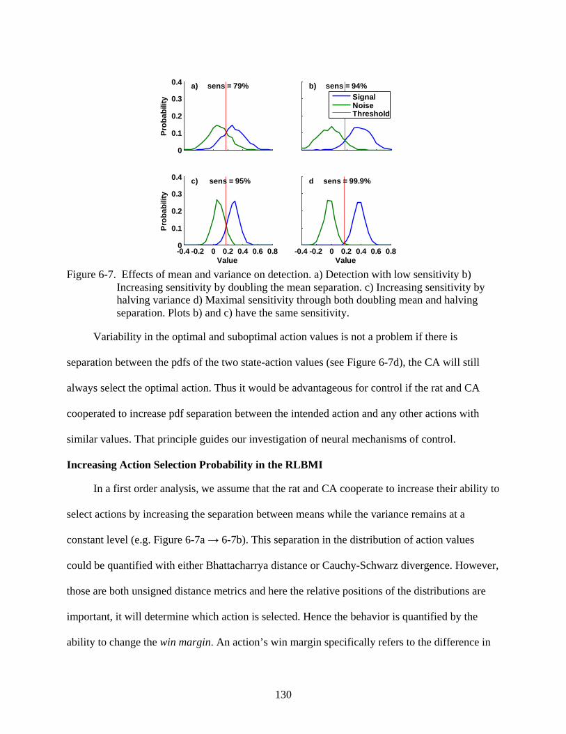
130

0

0.1

0.2

0.3

0.4 a) sens = 79%

Prob

abili

ty

b) sens = 94%SignalNoiseThreshold

-0.4 -0.2 0 0.2 0.4 0.6 0.80

0.1

0.2

0.3

0.4 c) sens = 95%

Prob

abili

ty

Value-0.4 -0.2 0 0.2 0.4 0.6 0.8

d sens = 99.9%

Value Figure 6-7. Effects of mean and variance on detection. a) Detection with low sensitivity b)

Increasing sensitivity by doubling the mean separation. c) Increasing sensitivity by halving variance d) Maximal sensitivity through both doubling mean and halving separation. Plots b) and c) have the same sensitivity.

Variability in the optimal and suboptimal action values is not a problem if there is

separation between the pdfs of the two state-action values (see Figure 6-7d), the CA will still

always select the optimal action. Thus it would be advantageous for control if the rat and CA

cooperated to increase pdf separation between the intended action and any other actions with

similar values. That principle guides our investigation of neural mechanisms of control.

Increasing Action Selection Probability in the RLBMI

In a first order analysis, we assume that the rat and CA cooperate to increase their ability to

select actions by increasing the separation between means while the variance remains at a

constant level (e.g. Figure 6-7a → 6-7b). This separation in the distribution of action values

could be quantified with either Bhattacharrya distance or Cauchy-Schwarz divergence. However,

those are both unsigned distance metrics and here the relative positions of the distributions are

important, it will determine which action is selected. Hence the behavior is quantified by the

ability to change the win margin. An action’s win margin specifically refers to the difference in

131

distribution means where the signal (win value) includes the action’s values when it was selected

and the noise (win boundary) includes values of whichever other actions were second highest

valued during the selections (see Figure 6-8).

500 1000 1500 2000 2500

0.05

0.1

0.15

0.2

0.25

0.3

0.35

0.4

Time [ms]

Valu

eBRFRUFLU

Figure 6-8. Win margin in the RLBMI. This segment of state-action values from Rat 1 shows

the components of the win margin calculation. The win margin is the average of win values are marked with ⊽ and the win boundaries are marked with △. The win margin for action BR includes examples of both actions FRU and FLU as the win boundary. The black traces are for the other 24 values.

The rat and CA can improve the win margin by increasing the win value and/or decreasing

the win boundary. Since the win-margin is only a first order statistic, it is unclear if variance is

causing the CA to select an unintended action when the win margin is low (e.g. Figure 6-8: times

800-1100). Larger win margins should make the action selection more robust if the variance is

constant (e.g. Figure 6-8: time 1600). The win margin should be correlated with the task

performance metrics assuming the rats have learned to select the necessary sequence of actions.

Changing the Win Margin through the VFE

The ability to change the win margin can be extracted from the VFE network because the

network adjusts its weights such that it is more sensitive to certain (e.g. task related) neurons and

less sensitive to less informative (e.g. non-task related) neurons. Sensitivity uses the network

132

weights and to quantify the magnitude of output changes given independent changes in the input

[58]. Prior researchers have used this concept to prune an ensemble of neurons from 185 to 41,

yet controlled a BMI to reconstruct trajectories with the same accuracy [58].

VFE sensitivity is calculated by taking the Jacobian of the output with respect to the input.

The VFE output is given in Equation 6-4 where t is the time index, Qk is the value (output) of the

kth action, si is the state (input) of the ith input tap5, and j is the index of the hidden processing

elements (see Figure 5-1). This sensitivity is given in Equation 6-5; however, there is a time

varying term si,t which was not present in [58]. This term arises from the difference in networks,

the VFE sensitivity includes the gradient of the nonlinearity. Additionally, the weights in the

VFE adapt over all time; therefore, each w term in Equation 6-5 can also include a time index as

in Equation 6-6. Both sensitivities have T values, where T is the number of samples in the BMI

experiment; additionally, both are truncated estimates of the gradient because the current state

can affect future weight changes.

( )∑∑ ∑ ⋅=

=

jjktj

jjkij

ititk wsnetwwssQ ,tanh)(

(6-4)

∑ ∑

⋅⋅=

∂∂

⋅∂

∂=

∂∂

jij

itiijjk

i

k

i

k wswwsh

hQ

sQ

,2sech (6-5)

∑ ∑

⋅⋅=

∂∂

jtij

ititijtjk

i

k wswwsQ

,,2

,, sech (6-6)

To create a concise descriptor, Si

∆wm was reduced to a single scalar for each neuron-action

pair which accurately reflects the change in VFE outputs. After testing multiple combinations of

the taps and of the time varying quantities in Equation 6-5 or 6-6, the combination that most

5 The RLBMI uses a gamma delay line (GDL) [120] (K = 3, µ = 0.3333) to embed 600 ms of neuronal modulation history into the state. Hence there are three taps per neuron.

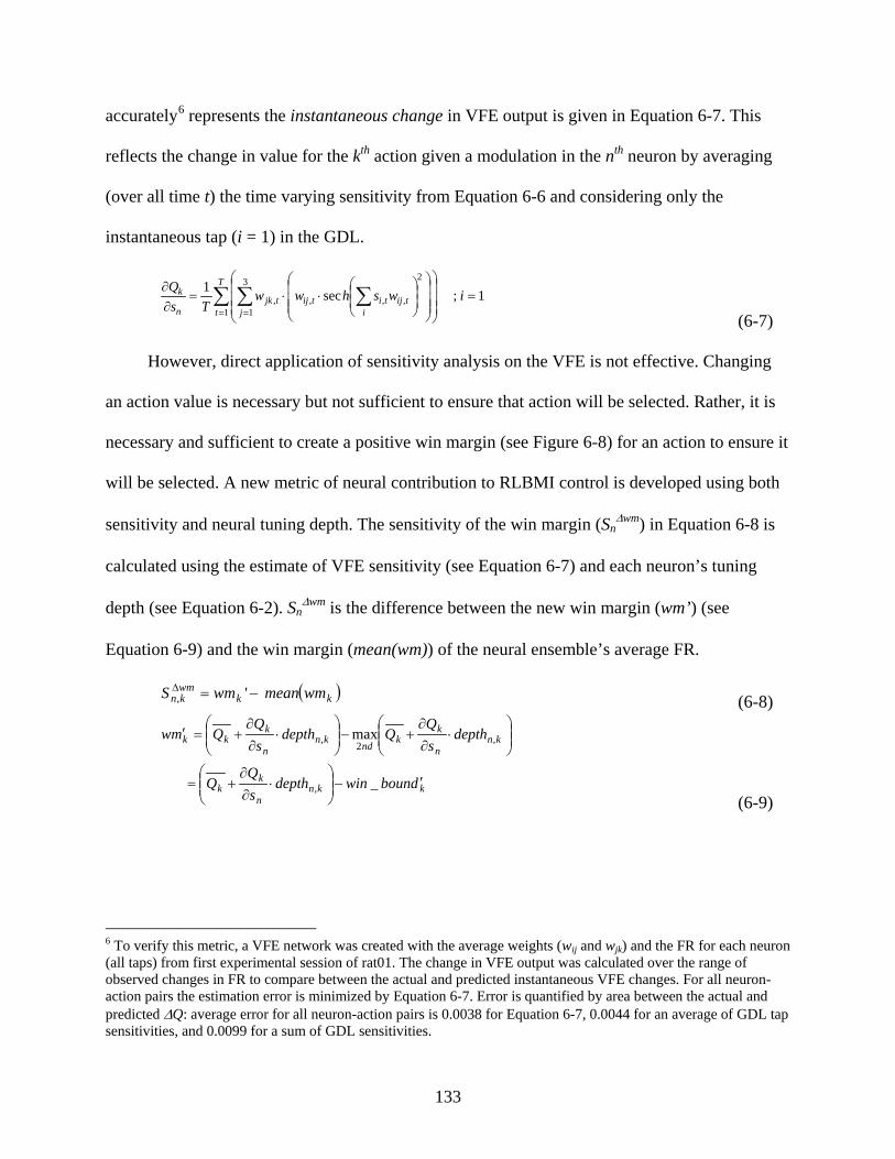
133

accurately6 represents the instantaneous change in VFE output is given in Equation 6-7. This

reflects the change in value for the kth action given a modulation in the nth neuron by averaging

(over all time t) the time varying sensitivity from Equation 6-6 and considering only the

instantaneous tap (i = 1) in the GDL.

1;sec1

1

3

1

2

,,,, =

⋅⋅=

∂∂ ∑ ∑ ∑

= =

iwshwwTs

Q T

t jtij

ititijtjk

n

k

(6-7)

However, direct application of sensitivity analysis on the VFE is not effective. Changing

an action value is necessary but not sufficient to ensure that action will be selected. Rather, it is

necessary and sufficient to create a positive win margin (see Figure 6-8) for an action to ensure it

will be selected. A new metric of neural contribution to RLBMI control is developed using both

sensitivity and neural tuning depth. The sensitivity of the win margin (Sn∆wm) in Equation 6-8 is

calculated using the estimate of VFE sensitivity (see Equation 6-7) and each neuron’s tuning

depth (see Equation 6-2). Sn∆wm is the difference between the new win margin (wm’) (see

Equation 6-9) and the win margin (mean(wm)) of the neural ensemble’s average FR.

( )kkwmkn wmmeanwmS −=∆ ', (6-8)

kkn

n

kk

knn

kk

ndkn

n

kkk

dbounwindepthsQ

Q

depthsQ

QdepthsQ

Qmw

′−

⋅

∂∂

+=

⋅

∂∂

+−

⋅

∂∂

+=′

_

max

,

,2

,

(6-9)

6 To verify this metric, a VFE network was created with the average weights (wij and wjk) and the FR for each neuron (all taps) from first experimental session of rat01. The change in VFE output was calculated over the range of observed changes in FR to compare between the actual and predicted instantaneous VFE changes. For all neuron-action pairs the estimation error is minimized by Equation 6-7. Error is quantified by area between the actual and predicted ∆Q: average error for all neuron-action pairs is 0.0038 for Equation 6-7, 0.0044 for an average of GDL tap sensitivities, and 0.0099 for a sum of GDL sensitivities.

134

Neural Contributions to Change the Win Margin

The contribution of each neuron to changing action win margins is estimated with

Equation 6-8. However, not all neurons are equally effective in selecting actions, i.e. normalizing

each S∆wm by the maximal S∆wm reveals the efficiency of each neuron. As in other BMI sensitivity

metrics, few neurons (19% – 24%) are most useful for the network in selecting actions. A caveat

is that individual contributions can not be superimposed to show the ensemble contribution. Only

33%, 40%, and 47% of the ensemble change in win margin for each rat is created by summing

individual changes. This problem arises because Equation 6-9 requires all other neurons remain

at their mean value which is unrealistic because that value is a mixture of neural states. However,

the metric still highlights a subset of neurons which are exploited by the VFE network.

Figure 6-9 focuses on the neurons identified as maximally efficient for each action. For all

rats, one neuron was most efficient for selecting two actions; another neuron was most efficient

for selecting the remaining action. The tuning depth confirms that the VFE can learn to exploit

both excitation and inhibition of neural firing (e.g. rat 1 n10) to control different actions.

Alternatively, the VFE can follow the more classic concept of tuning direction [54], using

excitation of neural firing (e.g. rat 1 n8) to select an action if the rat does not modulate that

neuron for other actions. Interestingly, in this session the rats were mostly likely to select one of

the two actions which were correlated with excitation and inhibition of the one set of neurons.

135

n10 n80

0.5

1

Rat

1

Max Normalized SdWM

n10 n8-5

0

5

10

Tuning Depth [Hz]

Act BRAct FRUAct FLU

n17 n11-1

0

1

Rat

2

n17 n11-10

0

10 Act BLAct FAct FRU

n21 n7-0.5

00.5

1R

at 3

Neuronn21 n7

0

10

20

Neuron

Act LAct FRUAct FLU

Figure 6-9. Maximum normalized neural contribution to win margin & tuning depths. The

neurons were indentified with Equation 6-8 in the final session of the 2nd difficulty.

This sensitivity to win margin metric provides further evidence that the rat and CA engage

in synergistic behavior because the most sensitive neurons also have significant differences in

neuronal modulations and typically the largest depth (Equation 6-2). It uses first-order statistics

of the separation between the selected action-value and the remaining values. As stated earlier,

this separation can be described more completely with the Cauchy-Schwarz (CS) Divergence

[161], which accounts for both mean and variance. Sensitivity of the CS divergence can also be

extracted from the VFE network, but it is much more abstract to interpret. Preliminary results

suggest that it highlights the same subset of neurons.

Co-evolution of RLBMI Control

A novel aspect of the RLBMI experiments was operation over multiple days in a changing

environment without disjoint network retraining. Therefore, the smoothly adapting VFE weights

contained partial information of the prior control strategy over days while also adapting towards

new strategies. This is a paradigm shift compared to other BMI architectures which require

retraining and may lose prior strategies before each use [8, 10, 50]. The rats all maintained

136

performance significantly above chance (details in [86]); however, the task completion

performance metrics (PR) decreased over most sessions as shown in Figure 6-10. However, as

noted in Chapter 5, this decrease parallels classic psychometric curves which show decreasing

performance as a task becomes more difficult in a variety of paradigms [119]. We highlight the

co-evolution of control with the features identified in this chapter such that learning is not

obscured by the decreasing PR.

Action Selection Correlation with RLBMI Performance

The average PR decreased in 89% of the sessions after a difficulty increase (vertical red

lines in Figure 6-8), e.g. rat 1, session 6. However, 71% of the time the rat and CA were able to

increase average PR within the same difficulty7, e.g. rat 2, session 2-3. This improvement shows

that RLBMI learning requires practice and benefits from a relatively stable environment. Other

BMI have also shown the same improvement with practice [59, 153] in a stable environment.

However, the RLBMI is learning in a novel environment without disjoint retraining; BMI prior

to this experiment had not demonstrated this ability.

At a high level of abstraction, each rat’s control strategy is partially reflected by the action

selection probabilities given in Figure 6-11. The rats need to select the proper sequence of

control actions for each task: PR will not improve if the CA helps the rat to efficiently select

incorrect actions. Comparison of Figures 6-10 and 6-11 reveals that large changes in the

distribution of p(action) correlated with large changes in PR. For example, in rat 3 (sessions 7-8)

there is a dramatic reorganization of the p(action L) and p(action FRU) in Figure 6-11. This

correlates with a sharp drop in performance in Figure 6-10. When the probabilities reorganize

again for rat 3 in session 9, there is a sharp increase in performance.

7 When only one session was present, the difficulty level was excluded from analysis (e.g. rat 1, 3rd difficulty).

137

5 10

40

50

60

70

80

90

100

Ave

rage

Per

cent

Rew

ards

Rat 01

Session2 4 6

Rat 02

Session2 4 6 8

Rat 03

Session

L trialsR trialsmeanDifficulty

Figure 6-10. RLBMI task performance. Percentage of tasks completed for left and right trials

over all sessions of use. This expands on Figure 5-5 which averaged performance over task difficulties. The red vertical lines represent a change in the environment.

5 100

0.1

0.2

0.3

0.4

0.5

0.6

0.7

0.8

0.9

1

p(A

ctio

n Se

lect

ion)

Session

Rat 1

Act BRAct FRUAct FLU

2 4 60

0.1

0.2

0.3

0.4

0.5

0.6

0.7

0.8

0.9

1

Session

Rat 2

Act BLAct FAct FRU

2 4 6 80

0.1

0.2

0.3

0.4

0.5

0.6

0.7

0.8

0.9

1

Session

Rat 3

Act LAct FRUAct FLU

Figure 6-11. Probability of action selection over sessions. There are no data-points for Rat 3

FLU for sessions 8-9 because that action was never selected. The red vertical lines represent a change in the environment.

Across all rats there is a general trend that more balanced action selection probability

correlates with higher performances. Examples are rat 1 session 5, rat 1 session 3, and rat 3

sessions 9. This is intuitive because Figure 6-11 is the probability over all trials, half of which

should be to the left and the other half to the right. In instances when one actions is nearly always

138

selected (e.g. rat 1 session 7), performance on that side (in this case L) increases but performance

on the other side crashes.

Potential Causes of Changing Action Selection

The evolving p(action) in Figure 6-11 is interesting but does not reveal the cause of these

actions selections. Due to the coupling of control, multiple issues may have caused the changes:

• The rat (having learned the task) attempts to select these actions by more frequently using neural modulations which have selected the action in the past.

• The rat may change neural firing rates for the actions it wants to select.

• The CA may adjust the weights of the VFE to make the efficient neurons more efficient (increase S∆wm) for selecting actions.

• The VFE may evolve to a state where certain actions become unavailable.

The first two concepts both involve the rat’s strategy. In the first section of this chapter, we

showed that the percentage of neurons which encoded some representation of robot actions (see

Figures 6-1 to 6-3). This change in the neuronal representation likely affected the action

selection. Here, we investigate how the rats adapted firing rate and how that (along with the CA

adapting weights) affected S∆wm. Additionally, we show how the VFE can reach a state where

actions are no longer accessible for the rat.

Evolution of sensitivity to win margin

Figure 6-12 focuses on the two neurons (for each rat) which were previously identified as

most efficient for selecting actions (see Figure 6-9). The top rows contains the neurons which

were efficient in selecting one action and the bottom rows contains the neurons which were

efficient in selecting the two different other actions. Unlike prior plots, the tuning depth is not

presented because it is unclear whether tuning depth (Equation 6- 2) changes due to a change in

mean FR, a change in conditional tuning (see Equation 6- 1), or a combination of the two factors.

139

5 10

10

20Rat 1, Neuron 10

FR [H

z]

5 100

0.51

SdWM

Session

5 105

1015

Rat 1, Neuron 8

FR [H

z]

5 100

0.51

SdWM

2 4 65

1015

Rat 2, Neuron 17

2 4 60

0.51

Session

2 4 6102030

Rat 2, Neuron 11

2 4 6

00.5

1

2 4 6 8102030

Rat 3, Neuron 21

2 4 6 8-0.5

00.5

Session

2 4 6 8

2040

Rat 3, Neuron 7

2 4 6 80

0.51

Act L

Act FRUAct FLU

Act BL

Act F

Act FRU

Act BR

Act FRU

Act FLU

Figure 6-12. Evolution of neural tuning and S∆wm. Tuning of the six neurons from Figure 6-9 are

presented in rows one and three over all sessions. Below each neuron is that neuron’s ability (normalized over all sessions) to change the win margin. Thicker traces are neuron action pairs identified as maximally efficient in Figure 6-9, thinner traces are the remaining pairs.

The tuning in Figure 6-12 suggests a changing neural modulation strategy for all three rats.

This change in strategy is also reflected in the S∆wm for these neurons (the 2nd and 4th rows of

Figure 6-12) which also changes over sessions. For the neuron-action pairs identified as efficient

(thicker traces) the mean absolute correlation between the tuning and S∆wm is 0.76. The absolute

correlation is used to include high negative correlations8. For the neuron action pairs not

identified as efficient (thinner traces) the mean absolute correlation is 0.51.

These results show that the rat and CA both adapted (either tuning or weights) over

sessions. For neurons only sensitive to one action, the sensitivity increased over sessions (1st

8 E.g. Rat 3, neuron 21, action FRU: CC = -0.97. This was the only negatively correlated efficient neuron-action pair

140

row). For neurons sensitive to two actions (3rd row), the sensitivity decreased. However, other

neurons became more efficient to overcome this problem. Sensitivity is also adversely affected

when the tuning depth sign changes (e.g. Rat 3, session 7-9) relative to earlier sessions.

Co-evolution towards action extinction

The final unexplained RLBMI phenomena are the changing control strategies of rats 2 and

3. The p(act F) and p(act FLU) trends to zero in later sessions for rats 2 and 3 respectively (see

Figure 6-11). The prior subsection showed (Figure 6-12) that both rats had neurons which where

increasing tuning, tuning depth, and S∆wm for those actions over sessions until the actions were

not selected. While it is possible the rats stopped trying to select those actions, it seems more

likely that a combination of VFE network training and changing conditional tuning of specific

neurons prevented selection of these actions.

As described in chapter 5, the VFE is trained over two orders of magnitude more on the

initial data (session 0) than it is trained on any other session. Additionally, the learning rates

were attenuated as difficulty increased to help maintain stable control [86]. Table 5-1 showed

that the input and output layer learning rates were attenuated to 45% and 31% of their initial

values by the final session. These two factors create a VFE with state projections that were set

for the initial data and adapt more slowly each session.

Figure 6-13 (top row) shows the mean value and winning value of the action that was

selected less often over time for each rat along with the other possible actions. In both rats 2 and

3, there was at least one neuron with a mean FR that was highly correlated to the mean action

value. These neurons were also efficient in selecting the actions and increased their tuning depth

over sessions. However, the mean FR for these neurons both dropped over sessions (see Figure

6-13, 2nd row) and eventually the average action values were below the ‘noise floor’ of the other

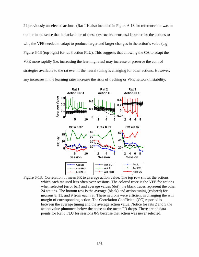
141

24 previously unselected actions. (Rat 1 is also included in Figure 6-13 for reference but was an

outlier in the sense that he lacked one of these destructive neurons.) In order for the actions to

win, the VFE needed to adapt to produce larger and larger changes in the action’s value (e.g

Figure 6-13 (top-right) for rat 3 action FLU). This suggests that allowing the CA to adapt the

VFE more rapidly (i.e. increasing the learning rates) may increase or preserve the control

strategies available to the rat even if the neural tuning is changing for other actions. However,

any increases in the learning rates increase the risks of tracking or VFE network instability.

Act BRAct FRUAct FLU

Act BLAct FAct FRU

Act LAct FRUAct FLU

5 100

0.1

0.2

0.3

Ave

rage

Val

ue

Rat 1Action FRU

5 105

10

15

FR [H

z]

Session

CC = 0.37

2 4 60

0.2

0.4

Rat 2Action F

2 4 6

10203040

Session

CC = 0.91

2 4 6 8-0.2

00.20.4

Rat 3Action FLU

2 4 6 8

20

40

60

Session

CC = 0.87

Figure 6-13. Correlation of mean FR to average action value. The top row shows the actions

which each rat used less often over sessions. The colored trace is the VFE for actions when selected (error bar) and average values (dot), the black traces represent the other 24 actions. The bottom row is the average (black) and action tuning (colored) for neurons 8, 11, and 9 from each rat. These neurons were efficient in changing the win margin of corresponding action. The Correlation Coefficient (CC) reported is between the average tuning and the average action value. Notice for rats 2 and 3 the action value plummets below the noise as the mean FR drops. There are no data-points for Rat 3 FLU for sessions 8-9 because that action was never selected.

142

Conclusions

This chapter began with four interesting aspects of RLBMI control. Each aspect was

revealed by analyzing both the rat and CA (through the VFE network) at a lower level of

abstraction. There were significant differences in neural tuning for almost 90% of the recorded

neurons which shows that there is a representation of robot actions in each rat’s neural

modulation. Analyzing the control mechanisms of the CA revealed that the VFE output was

consistent with principles of reinforcement learning but not optimally efficient for all rats. The

insight gained in analyzing the CA will be important for future RLBMI design. The performance

deficiencies reveal areas that need improvement in order to approximate return: VFE training,

CA policy, and the neural state.

The concept of win margin sensitivity to individual neurons revealed a small subset of

neurons which were more efficient for control. This subset of neurons also had significantly

different firing rates for different actions. It is possible that the CA adapted VFE weights such

that the win margin was most sensitive to this subset of neurons. Alternatively, rat may have

increased the neural tuning for those neurons which (through the VFE) were most efficient in

selecting actions. In either case, the rat and CA acted synergistically to select actions.

Finally we quantified the co-evolution of the rat and CA existed in these experiments. It

was addressed using the concise set of descriptors and neurons that were identified in the prior

sections. We found that both the tuning and sensitivity evolved over the course of control. VFE

network conditions which partially explained abnormal aspects of control were also indentified.

The insight into these mechanisms and conditions will enhance future user’s abilities to evolve

with and maintain stable control of the RLBMI.

This chapter also has thought provoking implications for understanding neural control

through a BMI. Here we used or modified existing analysis techniques to show co-evolution

143

mostly at the level of individual neurons. This work is important for two reasons: it was

unknown a priori how control was achieved and any new analysis metric must be benchmarked

against the existing standards anyway. Given that there is co-evolution of control, it is very

interesting to consider more advanced analysis techniques and what insight they may provide.

For example, the entire neural vector could be used to understand how rotations affect control or

how the VFE network segments the state.

The general implications for BMI designers are also interesting. We have shown that the

action representation increased over time. This may represent recruiting more neurons as the rat

practices prosthetic control to improve performance. Additionally, we found a common (relative

to each neuron’s unique mean firing rate) change in firing across both hemispheres for the

selected control actions. The rats learned to selection actions both with inhibition and excitation.

Similar control via excitation and inhibition has recently been reported in a different paradigm in

[153]. Finally, the RLBMI were able to co-evolve in changing environments without disjoint

retraining; BMI prior to this experiment had not demonstrated this ability.

144

CHAPTER 7 CONCLUSIONS

Overview

To this day, I remain impressed with my peers’ work in the fields of BMI/ BCI. Regardless

of any clinical implementation limitations, from my perspective it is amazing to develop

machines which learn to translate neural signals to prosthetic control. These machines are

provided a neural input which is at the scale of milliseconds, uses a code that is still not fully

understood, changes statistically over time, and is distributed across a space that is too large for

most humans to even consider. This input represents a gross sub-sampling of contributing

neurons. The machines then approximate a dynamic and nonlinear motor control system(s) to

control a prosthetic; sometimes accounting for radical translations1. The engineering behind

these accomplishments shows the ingenuity, determination, and skill of BMI developers.

This incredible BMI technology unfortunately remained in the lab and was difficult to

deliver to the clinical population. One company (Cyberkinetics) tried to commercialize and

deliver BMI (SL-based) to the clinic to much fanfare [50], but now is on the brink of bankruptcy.

We developed a novel BMI to achieve what I judged the most important issue for the clinic –

overcoming the need for a desired signal. We built on prior BMI contributions and also

incorporated concepts from both animal [119] and machine [103] RL theory. In the process, the

BMI paradigm was fundamental shifted and multiple implementation issues were addressed. The

RLBMI is still emerging and evolving, but it has capability to overcome these problems:

1. Finding an appropriate training signal in a clinical population of BMI users 2. Maintaining user motivation over length BMI training to master control 3. Relearning control whenever the neural signal or environment is non-stationary

1 In the RLBMI the robot would be at least five stories tall if the rat and robot were both scaled up to human size. The robot in the multi university DARPA grant led by Nicolelis was also larger than the monkeys using it.

145

Novel Contributions

In shifting the BMI paradigm away from SL ideologies, we have definitely made two

novel and substantial contributions to the state of the art. The first is a BMI that does not require

a desired signal (user movements) to learn. The second is a co-adaptive system that does not

require retraining before each new control session despite changing environments. Theoretically

we have also made a third contribution of decreasing the amount of time necessary for a BMI

user to master control but this must be validated in control studies. However, the RLBMI

architecture inherently facilitates this contribution.

The ability of the RLBMI to learn in a semi-supervised fashion without a desired signal

was clearly shown throughout this research (simulations and in vivo). The RLBMI completed

reaching tasks with only neural signals and a scalar reward modeled on the rat’s perception of

task completion. There was never a desired signal or proximity detector to teach the CA which

actions to use, instead only a post hoc reward to inform the CA of a good or bad job.

Reward is a powerful concept that represents a shared goal and exists simultaneously for

the BMI user and CA; both use a similar learning mechanism (RL). Hence, conceptually both

intelligent entities will co-adapt synergistically based on interaction with their respective

environments to master prosthetic control more rapidly. Additionally, this research advanced the

concept of shaping to achieve BMI control. Both synergistic co-adaption and shaping logically

enables development of complex tasks while possibly also reducing the “learning curve” for

BMI use. Control studies should validate the existence and significance of this contribution.

Finally, the rat model clearly demonstrated that this RLBMI can be used without separate

retraining periods. Retraining may create learning confounds because it generates a different

control mapping (network weights) for the user each day. Retrain will also create some delays

before the BMI can be used. RLBMI instead used continuous co-adaption over 6-10 days with all

146

training using a purely brain controlled prosthetic. Continuous co-adaptation can adjust to

changes in the environment(s) while also preserving prior prosthetic control experience.

The computation complexity for online RLBMI updates is on the order of a MLP. Coupled

with optimized signal acquisition and IKE for robot control, it met real-time implementation

deadlines: keeping the RLBMI on par with other BMI. This relatively low computational burden

is advantageous for low-power BMI applications. However, RLBMI has the distinct benefit of a

co-adaptive, reward-based learning which spawns the three contributions to the BMI field.

Additionally, the RLBMI was analyzed in terms of user (rat) and CA contributions and

cooperation. A conditionally tuning metric showed that each rat significantly changed neural FR

between at least two of the control actions. Detailed VFE network analysis showed that it was

exploiting information in the reward signal but the training could be optimized to overcome

some errors. A new metric was developed to specifically show the effect of neural modulations

on action selection based on the VFE network weights. This metric and the other analysis

provided opportunities to quantify to co-evolution of RLBMI control. In summary, there are four

contributions from this work:

1. A RLBMI which does not need an explicit desired signal.

2. A RLBMI which improves performance with usage which may allow for more difficult tasks (or faster task mastery) due to the feedback and co-adaptation between the user and the CA.

3. A RLBMI which does not require separate re-training before each prosthetic control session.

4. A set of analysis techniques which reveals detailed individual and collaborative performance of the user and CA in this RLBMI.

Implications of Contributions

Reward-Based Learning in BMI

This contribution alone motivated my entire research path. The RLBMI facilitates

restoration of functional limb ability through prostheses without requiring paralyzed or amputee

147

BMI users to make physical movements to train the BMI controller. This ability is critical

because those users cannot make the movements. Though the RLBMI is still an emerging and

evolving architecture, its inherent qualities are a major step to moving BMI technology from the

laboratory to clinical implementation. The RLBMI learns from interactions with the

environment; this learning philosophy eliminates (or reduces) the need for a technician. Learning

from the environment also allows the BMI to learn continuously, even in brain-control.

Learning to achieve a goal by taking actions which have previously been beneficial for us

may seem familiar and logical. This familiarity is likely due to the prevalence of RL in the way

that we learn as humans. Additionally, even if the explicit details of achieving a goal is quite

complex, RL presents a sensible framework with the clear and simple objective of maximizing

return (see Equation 2-1). The complexity of the achieving a goal does not change this objective;

rather it is incorporated into the rewards that compose the return.

Although shifting the BMI paradigm from SL to RL drastically reduces the information

content in the error signal, it actually can become easier to add complexity to control strategies.

Consider a BMI user who had already learned prosthetic control decides he or she wanted to

adjust their strategy. For example, the BMI user desires to minimize commanded torque change

[112] because they know this will preserve the prosthetic’s batteries. The SL learn-via-

technician method would require inverse dynamics optimization [110] of a computational

prosthetic model to find one training trajectory that will minimize this cost [113]. This will have

to be repeated for as many trajectories as the user wants and any errors in the computational

model will propagate to control. The RLBMI designer can instead calculate torque change during

control and penalize the reward at each step by this quantity. The CA will adapt its control

strategy to minimize the penalties without any other user or technician intervention.

148

Reduced User and BMI Training Requirements

The ability of the RLBMI to co-adapt allows it to retain past experience while still

adapting to changes in the user’s neural modulations. Additionally, the RLBMI can adapt learn

new tasks based on interactions with the environment. This crucial feature allows the RLBMI to

be used day-after-day without retraining: introducing continuity in BMI control. Removing the

necessity of BMI retraining is another step toward increasing the appeal of BMI technologies to

the clinical population of users.

The synergistic co-adaptation in the RLBMI can reduce the amount of time necessary for a

user to master BMI control. This reduced training time would be enabling to the user – they

avoid wasting valuable time and limited energy. Potentially this creates a positive feedback

where the user actively controls the BMI for longer periods and has more opportunity to adapt

his or her control; then the CA has more opportunity to adapt to the user’s control strategy and

improves performance. Improved performance encourages even longer periods of user control,

which gives the user and CA more time to learn.

Co-Evolution of BMI Control

The general architecture of the RLBMI has amazing implications for control. Generally

control systems with two intelligent systems can have the problem of conflicting goals and

oscillating instability as the two systems adapt around each other. However, since both the

RLBMI user and CA have a shared goal and both use the same learning mechanism (RL) they

will act synergistically. This is a unique situation where the CA functions as an intelligent

assistant to help the user complete tasks.

Specifically, the three contributions to BMI design all facilitate the co-evolution of BMI

control shown in Figure 7-1. This idea is related to the shaping described earlier where the user

only would have to complete a part of the task and the CA would handle the rest. Eventually the

149

user could learn the entirety of the task. Again this synergistic behavior naturally arises because

it is in the best interest of both parties. The fourth contribution of quantifying user and CA

participation in RLBMI control allows visualization of this co-evolution. Furthermore, it may

facilitate adjustment of the rates of CA assistance (e.g. through VFE network learning rates)

based on the current contributions and cooperation of the user and CA.

Figure 7-1. Co-Evolution of BMI control in the RLBMI. In this case the user and intelligent

assistant (the CA) are attempting to reach the same goal (water).

The co-evolution has broad implications in clinical applications. One intriguing example is

a patient rehabilitation scenario. At first the patient may only have the strength to move a light

resistance over a trajectory with the CA providing the necessary extra strength. However, over

time the patient will learn more autonomous control and need less and less assistance from the

CA. Alternatively, the CA can provide tailored resistance/ assistance to the patient based on

whether the patient is following the limb motion strategies prescribed by the physical therapist.

In that case, CA does not even need access to brain signals, the limb will suffice.

150

Future RLBMI Developments and Integration

After achieving a fundamental shift in the BMI paradigm, one might expect a feeling of

satisfaction and closure. While I am very proud of our accomplishments there is no feeling of an

ending or even a pause. Instead there is a sense of excitement of all of the intriguing possibilities

that may arise through this co-adaptive architecture. This section previews some major themes

for future development.

Translating Rewards Directly from the User

In this work the rewards were programmed by the BMI designer, but in the future they will

be translated from activity in the user’s brain (such as striatum which is responsible for reward/

error prediction [162]). It is encouraging to see that the functional response of neurons in the

Nucleus Accumbens (NAcc is part of the ventral striatum) is similar to the externally

programmed Gaussian reward function around each target [163]. Hopefully this similarity will

facilitate seamless integration of the NAcc reward information into the RLBMI. When this is

achieved, the brain control of prosthetics could be made more general with the production of new

goals and reduction of old goals.

Incorporating Different Brain State Signals

BMI researchers and rehabilitation therapists currently extract neural information at a

variety of different levels of abstraction from different areas of the nervous system. To validate

the RLBMI, we used single unit activity in the primary motor cortex. However, there were no

constraining assumptions in the RLBMI that require neuron from MI or even single unit activity.

The RLBMI only requires a relatively repeatable state signals that corresponds to different

actions. Already this learning method has been adopted for a major European-based

collaboration in developing neuro-prosthesis for the vestibular system which is about to begin.

Hopefully the research community will continue to embrace this architecture and enhance it.

151

Expanding the Action Set

This work used a relatively simple action set to move a prosthetic end-point in Cartesian

coordinates. However, the RLBMI also does not make assumptions which constrain the action

set to a certain style or coordinate system. The only requirement is that the action provides

feedback and utility for the user. Hence, expansion is possible depending on the complexity of

the prosthetic (e.g. cursor vs. FES system). Additionally, the action set may include complex

movements or motion basis as explored in Chapter 2.

Developing a New Training Mechanism for Unselected Actions

One common problem that we have seen in all users of the RLBMI and in simulations is

the attenuation of the 27 member action set to 2-4 actions after training. Although we have

provided multiple explanations for why the rat may benefit from this reduced set (e.g. visual

feedback, reduced number of neural states to generate, using the simplest solution in a two target

choice task) we also need to consider if this set attenuation is imposed by the experimenter.

Chapter 5 discussed the concept that unselected actions do not generate a return (Rt) and

thus they are not updated because Rt is undefined (the eligibility trace acts partially to set the

learning of unselected actions to zero). Chapter 6 showed that maintaining a group of undefined

actions is not optimal and can lead to instability in the VFE network and robot control. This

limited action set arises because the CA trains the VFE to set the value of a few actions much

higher than the rest of the actions (e.g. Figure 6-8). The low valued actions will likely never be

selected unless the high valued actions repeatedly fail. However, the first low valued action to be

selected will not necessarily be the next best because it is undefined.

The current state of the VFE also prevents solving this problem with a soft-max policy

which updates the next best actions through directed exploration (Chapter 2). Since only few

152

actions are highly valued, the next best will likely be in the wrong direction (assuming one high

value action per target). This explains why soft-max policies were unstable in this application.

The principled solution would be to use a model-based RL with an estimator for future

neural states. Then, the RLBMI operating procedure in Chapter 5 would be followed for one

action to move the robot; additionally, it would be simulated for the 26 unselected actions.

Through simulations both rt+1 and st+1 are available; hence the action values are no longer

undefined and can be updated. The difficulty is creating accurate predictors of future neural

modulations in the 16-29D neural ensemble. However, it may be possible instead to predict the

3D hidden layer output in the VFE network. Then at least the output layer of the VFE network

could be trained via simulations. This all hinges on the quality of the hidden layer predictor.

Another solution is to distribute the current VFE learning mechanisms to other unselected

actions. First we need to assume that the neural state transitions (see Equation 2-7) will be

similar after taking similar actions; then future states will be similar. After calculating the actual

error (Equation 5-3), the eligibility trace (Equation 5-6) should be adjusted such that similar

action are also partially updated. A direct way to do this is to use the distance between possible

action endpoints, similar to the neighborhood update in a Kohonen Self Organizing Map (SOM)

[145]. This provides the RLBMI user the opportunity to select from a larger population of

actions and like the SOM the neighborhood could be annealed over time to refine the updates.

Refining the RLBMI Parameter Set to Balance Control

A challenge of the RLBMI was to manage both a high dimensional parameter set and two

coupled, intelligent systems learning together. We found a set of parameters that facilitated

control for all three rats and more detailed analysis in Chapter 6 found descriptors which

revealed the contributions of both the rat and CA to control. With this added insight, the

153

experimental designer can make more informed decision to help him or her optimize the RLBMI

parameter set for a given application, user, and amount of requested CA assistance.

Advancing the Animal Model

Using the RLBMI in a rat model has attracted some criticism for being too difficult for the

rat or rats not providing a good foundation for translational research. We are confident that the

task is not too difficult because multiple rats have demonstrated prosthetic control. The only

change to the paradigm that should help is to also incorporate more auditory feedback for the rat

to localize the robot and targets. However, there was a major problem with the rat model of

extinction – rather than seeing failure as bad, the rat learned a new task or forgot the old task.

After multiple unsuccessful (rat was only successful for one target) sessions with one rat,

there were significant changes in the peri-event histograms of neural firings. The neuronal

modulation pattern was very different than earlier sessions. Since the rat earned a reward in half

of the trials regardless of its involvement, it was hypothesized that there had been some

extinction of the rat’s knowledge of the task. To combat this, each session (for rats 2 and 3)

begins with 12-25 physical control trials. None of the neural data in these trails was used to

update the RLBMI, physical trials were only designed to engage the rat and prevent extinction.

These trials did improve overall performance and seemed to prevent extinction. This rat model

involves at least six weeks of preparation before a single experiment can be run, it is crucial that

BMI control does not cause extinction. We hypothesize human users would not require such

techniques to maintain engagement because humans would be more cognizant of the task.

Quantifying the Relationship between Neuronal Modulations and RLBMI Performance

Although the random walk model is used very often in prominent BMI publications, in

Chapters 2 and 5 the CA was clearly able to learn to perform better than the random walk

predicted even in the absence of state information. In adapting the VFE, the CA adjusts the

154

randomness of action selection, typically learning to follow whichever actions randomly led it to

a first reward. Performance will be nearly perfect for one target and nearly zero for the other

(Figure 5-5); this is the lower bound for the RLBMI (a random walk sets the lower bound in a

non-learning algorithm). However it would be interesting to know more than the bounds

It is possible to instead find a functional relationship between the repeatability of neural

modulations and performance if artificial neural data is created. This relationship will set a more

realistic upper and lower bound for a given neural modulation repeatability. Although it does not

directly help train the network, it provides a descriptor for evaluating training and allows the

experimenter to predict the quality of the user’s neural signal based on the RLBMI performance.

Implementing Advanced RL Algorithms

The RLBMI used a model-free RL technique because environmental dynamics were

unknown. The CA can only learn from experience and cannot predict future states. To overcome

the known limitation of relatively (compared to supervised-learning) slow learning speed, the

available data was reused in multiple-epoch, offline VFE training. Initially (session 0) the user

was given a random VFE to avoid long training which seems more a hack than a principled

solution. However, believe that through the Cyber-Workstation [134] (see Chapter 4) this

RLBMI has the potential to rapidly adapt the VFE even from random, co-adapting with the user.

Future RLBMI implementation also may benefit from model-based RL that includes an

environmental model to estimate future states and rewards [103]. This modification would allow

the CA to learn from both experience and model prediction of possible environmental

interactions; thus facilitating faster learning. Additionally, finding explicit functional

relationships between states, actions, and reward could provide some insight into how the

different brain areas may process and share information. These types of relationships address the

core of the action-perception cycle in human sensory processing and decision making.

155

APPENDIX A DESIGN OF ARTIFICIAL REWARDS BASED ON PHYSIOLOGY

Introduction

This appendix provides further details about the exact positions of the target levers and

starting robot position for the brain control task. Furthermore it explains the external reward

functions created for the CA in Equations 3-2 and 3-3. This CA reward is imposed by the

experimenter; however, it is designed to approximate the physiological rewards that the user is

experiencing.

Reference Frames and Target Lever Positions

There is a global reference frame on the countertop directly under the center of the robotic

mount. The x-axis extends to the right from rat’s perspective. The y-axis extends forward

towards the robotic levers. The z-axis extends vertically towards the robotic mount. There are

two target lever reference frames with the same orientation as the global frame but originating at

the target robot levers (left and right).

Table A-1. RLBMI robot workspace landmarks x [cm] y [cm] z [cm]

Robot initial position 0.00 12.00 14.00 Left target lever -8.00 36.74 25.85 Right robot lever 8.00 36.74 25.85

Coordinates are in the global reference frame

Approximating User Reward

Ideally, the CA would monitor reward from the actual user to determine when the user was

satisfied that a task was completed. Although regions such as striatum process information about

reward and error prediction [162], a reliable recording and extraction of reward signals from this

area is not yet available1. Furthermore, fixing the reward to some known constant values

1 Currently, a new RLBMI architecture which exploits the users reward signal is being developed by Mahmoudi

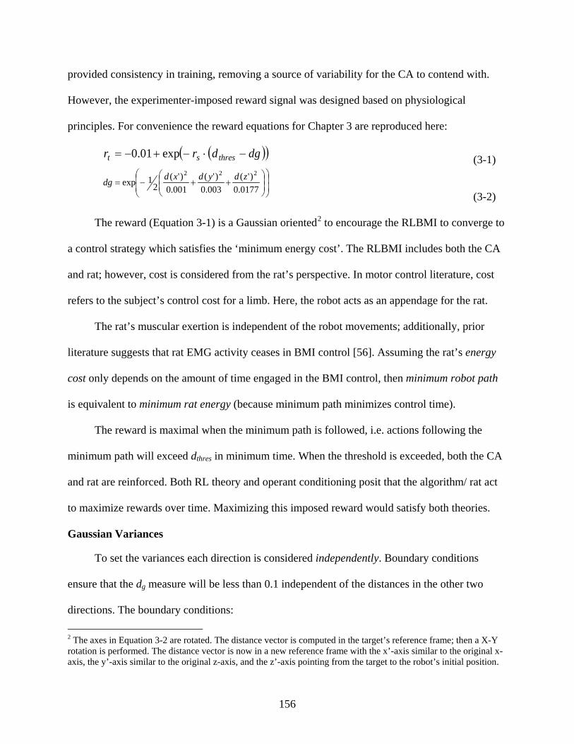
156

provided consistency in training, removing a source of variability for the CA to contend with.

However, the experimenter-imposed reward signal was designed based on physiological

principles. For convenience the reward equations for Chapter 3 are reproduced here:

( )( )dgdrr thresst −⋅−+−= exp01.0 (3-1)

++−=

0177.0)'(

003.0)'(

001.0)'(

21exp

222 zdydxddg (3-2)

The reward (Equation 3-1) is a Gaussian oriented2 to encourage the RLBMI to converge to

a control strategy which satisfies the ‘minimum energy cost’. The RLBMI includes both the CA

and rat; however, cost is considered from the rat’s perspective. In motor control literature, cost

refers to the subject’s control cost for a limb. Here, the robot acts as an appendage for the rat.

The rat’s muscular exertion is independent of the robot movements; additionally, prior

literature suggests that rat EMG activity ceases in BMI control [56]. Assuming the rat’s energy

cost only depends on the amount of time engaged in the BMI control, then minimum robot path

is equivalent to minimum rat energy (because minimum path minimizes control time).

The reward is maximal when the minimum path is followed, i.e. actions following the

minimum path will exceed dthres in minimum time. When the threshold is exceeded, both the CA

and rat are reinforced. Both RL theory and operant conditioning posit that the algorithm/ rat act

to maximize rewards over time. Maximizing this imposed reward would satisfy both theories.

Gaussian Variances

To set the variances each direction is considered independently. Boundary conditions

ensure that the dg measure will be less than 0.1 independent of the distances in the other two

directions. The boundary conditions: 2 The axes in Equation 3-2 are rotated. The distance vector is computed in the target’s reference frame; then a X-Y rotation is performed. The distance vector is now in a new reference frame with the x’-axis similar to the original x-axis, the y’-axis similar to the original z-axis, and the z’-axis pointing from the target to the robot’s initial position.

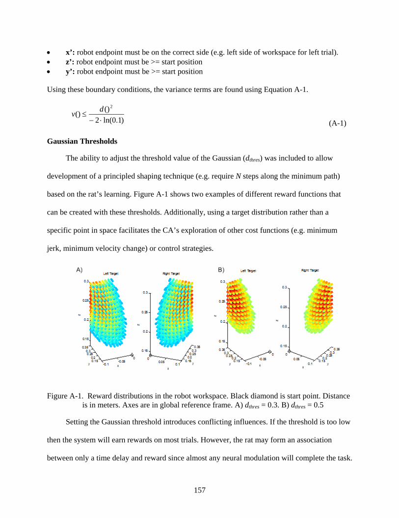
157

• x’: robot endpoint must be on the correct side (e.g. left side of workspace for left trial). • z’: robot endpoint must be >= start position • y’: robot endpoint must be >= start position Using these boundary conditions, the variance terms are found using Equation A-1.

)1.0ln(2()()

2

⋅−≤

dv (A-1)

Gaussian Thresholds

The ability to adjust the threshold value of the Gaussian (dthres) was included to allow

development of a principled shaping technique (e.g. require N steps along the minimum path)

based on the rat’s learning. Figure A-1 shows two examples of different reward functions that

can be created with these thresholds. Additionally, using a target distribution rather than a

specific point in space facilitates the CA’s exploration of other cost functions (e.g. minimum

jerk, minimum velocity change) or control strategies.

Figure A-1. Reward distributions in the robot workspace. Black diamond is start point. Distance

is in meters. Axes are in global reference frame. A) dthres = 0.3. B) dthres = 0.5

Setting the Gaussian threshold introduces conflicting influences. If the threshold is too low

then the system will earn rewards on most trials. However, the rat may form an association

between only a time delay and reward since almost any neural modulation will complete the task.

158

Additionally the CA learning will be hindered because almost every action sequence will be

reinforced. This situation represents a task which is too simple. Setting a high threshold will

avoid the potential problems listed above. However, very few trials will lead to a reward. The

animal may experience learning extinction, form false associations, or lose motivation. This

situation represents a task which is too difficult.

159

APPENDIX B BACK-PROPOGATION OF TD(LAMBDA) ERROR THROUGH THE VFE NETWORK

The VFE networks are MLPs (see Figure 5-1) which are trained on-line with TD(λ) error

(see Equation 5-4) via back-propagation. The cost is defined as squared TD(λ) error in Equation

B-1. The output layer weight update is given in Equation B-2 with two conditions. The first

condition is updating weights which are connected to the PE used to estimate the current state-

action value (Equation B-2a). Equation B-2b shows that weights that are not connected to the PE

used to estimate the current state-action value are not used. Similarly, Equation B-3 shows the

weight update for the input layer weights with two conditions to show how the errors are

propagated through the output layer weights depending on which output PE these errors are

coming from.

( )2

21)( λδ ttJ =

(B-1)

( )

jk

k

kOLjk W

QQ

tJtW∂∂

⋅∂∂

⋅−=∆)(α

(B-2) if at = ak

[ ]( )

( )( ) ( )( )thlf

hlf

jntT

nn

tOL

jtOL

T

ntOL

⋅+⋅=

⋅⋅=

+−+⋅⋅−=

+=

=

∑

∑

δγλδα

δα

δαλ

λ

1

10)100(

(B-2a) if at != ak

[ ]0

0)000(1

=

+−+⋅⋅−= ∑ =

T

ntOLλδα

(B-2b)

( )

ij

k

kILij W

hlhlhlf

hlfQ

QJtW

∂∂

⋅∂

∂⋅

∂∂

⋅∂∂

⋅−=∆)(

)(α

(B-3) if at = ak

iij

iijktIL swtsw ⋅

−⋅⋅⋅= ∑

2

)(tanh1λδα (B-3a)

160

if at != ak

0

)(tanh102

=

⋅

−⋅⋅⋅−= ∑ iij

iijkIL swtswα

(B-3b)

Without two further clarifications, Equations B-2 and B-3 are incomplete. Back-

propagation requires calculation of the error gradient with respect to the VFE weights. Equation

B-2a explicitly shows this calculation for the output layer weights assuming action k was

selected at time t. (If an action other than k was selected at time t, then ∂J/∂Q = 0.) The ∂J/∂Q

calculation in Equation B-2a assumes that only Q(t)k is dependant on the current Wjk; all future

Qk are not influenced by the current Wjk hence their gradient is zero. This assumption ignores the

dynamics of the system; truncating the true gradient. Instead the VFE climbs an approximate

gradient without explicit calculation [103, 116, 117, 143]. It is unclear how much learning could

be improved using back-propagation through time [91], but that investigation is beyond the

scope of this dissertation.

The other clarification necessary is that the network must be causal; yet, in all of the

update equations the TD(λ) error is used. Equation 5-4 showed that TD(λ) error requires

knowledge for all future TD(0) errors. With TD(λ) error, it is only possible to perform partial

weight updates (see Equations B-2 and B-3) based on the currently available TD(0) errors. To

illustrate this, consider the update to output layer weights assuming those weights are connected

to the PE corresponding with the actions taken. At time t+3 there would be sufficient information

to partially update the weights used for time t to time t+2. Equation B-4 shows the possible

partial updates given the current information at time t+3:

( ) ( ) ( )( )

⋅++⋅=∆ ∑++ ij

iitttOLjk wtstW )(tanh2

21

1 δγλδγλδα (B-4)

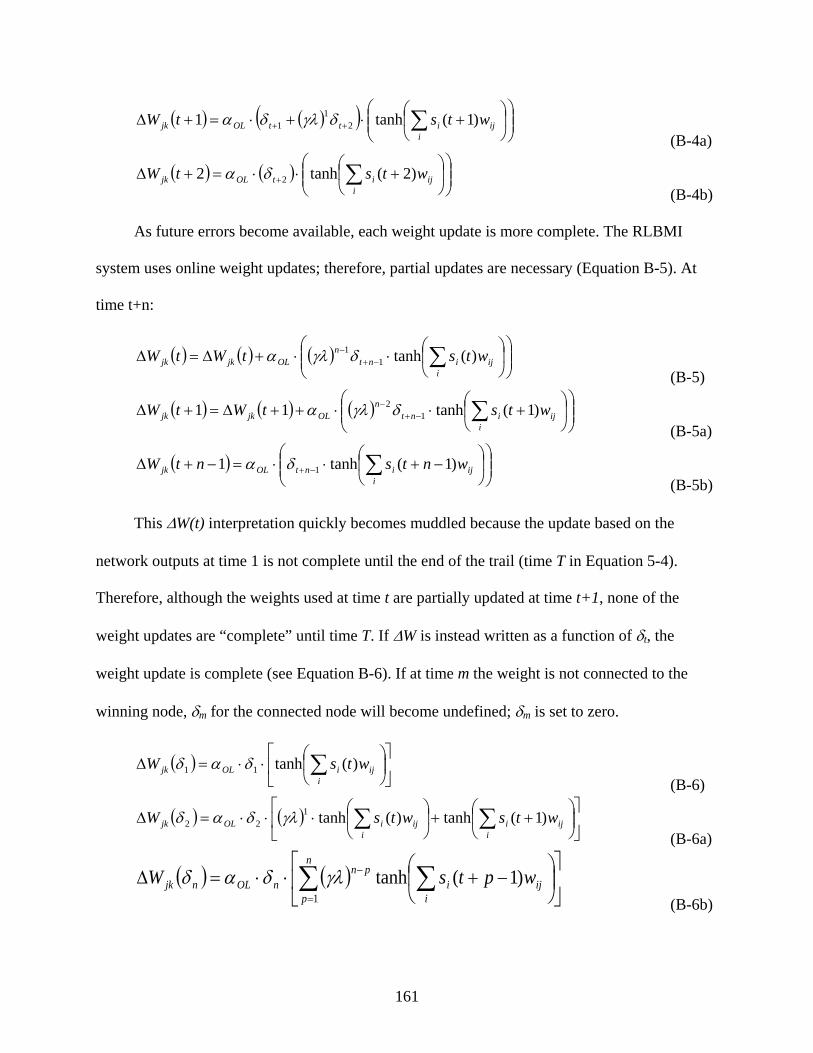
161

( ) ( )( )

+⋅+⋅=+∆ ∑++ ij

iittOLjk wtstW )1(tanh1 2

11 δγλδα

(B-4a)

( ) ( )

+⋅⋅=+∆ ∑+ ij

iitOLjk wtstW )2(tanh2 2δα

(B-4b) As future errors become available, each weight update is more complete. The RLBMI

system uses online weight updates; therefore, partial updates are necessary (Equation B-5). At

time t+n:

( ) ( ) ( )

⋅⋅+∆=∆ ∑−+

−ij

iint

nOLjkjk wtstWtW )(tanh1

1δγλα (B-5)

( ) ( ) ( )

+⋅⋅++∆=+∆ ∑−+

−ij

iint

nOLjkjk wtstWtW )1(tanh11 1

2δγλα (B-5a)

( )

−+⋅⋅=−+∆ ∑−+ ij

iintOLjk wntsntW )1(tanh1 1δα

(B-5b)

This ∆W(t) interpretation quickly becomes muddled because the update based on the

network outputs at time 1 is not complete until the end of the trail (time T in Equation 5-4).

Therefore, although the weights used at time t are partially updated at time t+1, none of the

weight updates are “complete” until time T. If ∆W is instead written as a function of δt, the

weight update is complete (see Equation B-6). If at time m the weight is not connected to the

winning node, δm for the connected node will become undefined; δm is set to zero.

( )

⋅⋅=∆ ∑ ij

iiOLjk wtsW )(tanh11 δαδ

(B-6)

( ) ( )

++

⋅⋅⋅=∆ ∑∑ ij

iiij

iiOLjk wtswtsW )1(tanh)(tanh1

22 γλδαδ (B-6a)

( ) ( )

−+⋅⋅=∆ ∑ ∑

=

−n

pij

ii

pnnOLnjk wptsW

1)1(tanhγλδαδ

(B-6b)

162

If the final term is removed from the sum, Equation B-6 can be rewritten as Equation B-7;

this format shows that our implementation is in agreement with Sutton’s original TD(λ) back

propagation formulation using eligibility traces [117].

( ) ( )

−++

−+⋅⋅=∆ ∑ ∑∑

−

=

−1

1)1(tanh)1(tanh

n

pij

ii

pnij

iinOLnjk wptswntsW γλδαδ

(B-7)

163

APPENDIX C INTERNATIONAL RESEARCH IN ENGINEERING AND EDUCATION REPORT:

CAMBRIDGE UNIVERSITY

Introduction

Brain-Machine Interface (BMI) is an active research topic with the potential to improve

the lives of individuals afflicted with motor neuropathies [9]. For the past eighteen years, the

Computational NeuroEngineering Laboratory (CNEL) at the University of Florida (UF) has been

pioneering the development of signal processing models used to translate neural activity into

behavior [164]. Our interdisciplinary group also includes the Neuroprosthetics Research Group

(NRG), and Advanced Computing and Information Systems (ACIS) Laboratory. We are

developing a Cyber-Workstation (C-W) to obliterate limitations currently faced by BMI

designers, i.e. the C-W provides tremendous remote computing power [165] yet still returns BMI

outputs (e.g. prosthetic commands) locally to satisfy real-time deadlines [137]. Furthermore the

C-W provides an integrated environment for efficient code development and repeatable analysis

of results [134, 135, 137]. This ground-breaking research is supported by the Dynamic Data

Driven Applications Systems (DDDAS) section of the National Science Foundation.

At the core of the C-W architecture is Wolpert and Kawato’s theory of motor control

which uses Multiple, Paired Forward and Inverse Models (MPFIM) [16]. MPFIM in an

intriguing theory that has been further refined but the idea of control via predictive modules has

remained intact [70, 166, 167]. The C-W is particularly suited to utilize MPFIM architecture

because the C-W exploits grid-computing to process the multiple sets of models in parallel.

Furthermore, it provides power and flexibility for BMI designers. Regardless of whether their

BMI incorporates MPFIM theory, the designer still has access to N (currently 10, but

expandable) sets of up to three interacting models in which he or she can place any algorithm.

164

A natural extension to our project was to broaden the impact by investigating the motor

control theory behind the C-W architecture. Specifically, movemes (motion primitives) have

been proposed as a basis set to compose all natural movements. We developed a method of

decomposing motion into movemes in joint-angle space [108], motivated by musculoskeletal

relationships which modulate force production, e.g. the force produced (and the response of the

limb) for a given neural activation depends on muscle states. The relationships are based on

muscle length, velocity, and moment arms which are completely described in joint angle space.

Theoretically, movemes could guide the initialization of C-W model sets, with one model set per

moveme. Despite the experimental [19, 85, 168, 169] and neuroscience [166, 170-172] support

for movemes, it was unclear whether movemes are intrinsic to motor control or an artifact of

experimental design.

Jack DiGiovanna was sent to investigate this phenomenon with Daniel Wolpert in the

Computational and Biological Learning (CBL) Lab (Cambridge University, England) from

October to December of 2007. Jack was a natural candidate because he was responsible for prior

movemes work [108]. As a 3rd year biomedical engineering graduate student, he was trained both

as a BMI designer and behaviorist. In the process of BMI design, he also has studied motor

control literature; hence was the most prepared student on our grant to start a dialogue with

members of the CBL lab.

Dr. Wolpert’s group is world renown for motor control system theory. They strive to

develop an understanding of how the brain achieves sensorimotor control of the human upper

extremity. An area of continued success is optimal control theory; here they have found an

optimal motor control loss function, methods of combining redundant muscles to reduce neural

control noise, and developed novel movement optimization cost functions. Bayesian probability

165

techniques are further improving motor control models. The lab has made advances in

understanding sensory attenuation based on predictive models, TMS, and motion. CBL also

works on the predictive models for different force fields - including model and control signal

interference, learning efficiency, linear model combinations, and appropriate coordinate systems.

Additional work is being done to show the relationship and cooperation between the visual and

motor brain systems in either visual, motor, or visuomotor tasks.

Before the trip, Wolpert’s lab had collected a dataset from the Natural Statistics project.

Multiple subjects had their arm positions instrumented during uninterrupted Activities of Daily

Life (ADL) for up to 4 hours at a time. This natural data provides a unique opportunity to

investigate movemes because it was unconstrained and should be free of experimental biases. A

set of movemes for the arm motions used in ADL would be a significant contribution both motor

control system theory and to future BMI development. We also expected the collaboration would

help us understand our closed-loop BMI results [86]. Our work is primarily driven by engineers;

however, Wolpert is a theorist and can help refine the motor control and learning concepts in our

work. The CBL would benefit from access to CNEL’s advanced BMI algorithms, signal

processing, and ACIS’s grid-computing infrastructure. Different perspectives and use of the tools

and ideas that we share would also encourage collaboration beyond the grant’s scope and length.

Research Activities and Accomplishments of the International Cooperation

Researchers at the Sensorimotor Control Lab collected unique datasets of natural

movements of the arm and hand. The arm dataset was more applicable to prior work [108], but it

only included elbow flexion angle and relative elbow and wrist positions because the purpose of

their study was to investigate symmetric and anti-symmetric movements of the subject’s arms.

Hence, there was insufficient information to analyze the arm in joint-angle space. The hand

dataset is comprised of 6 subjects, each recorded for an average of 170 minutes. A laptop worn

166

in a backpack recorded from an instrumented CyberGlove (Virtual Technologies, Palo Alto, CA)

to obtain 19 Degrees Of Freedom (DOF). The DOF included: flexion in all joints of each of the

five digits (14 DOF), thumb abduction (1 DOF), and relative abduction between the fingers (4

DOF). The sampling rate was 84 Hz and average sensor resolution was 0.6 +/- 0.2 degrees [173].

The hand study originally investigated Principal Components (PC) of movement to compare with

prior laboratory studies and determine if additional control strategies were necessary for ADL.

The hand dataset provided the most complete recording of natural movements and included

sufficient DOF to completely translate movements into the joint angle space [108]. For

clarification, joint angle space refers to a data projection where each dimension represents one

joint angle (e.g. index finger distal inter-phalanges flexion). Recordings from two subjects were

used explore the hand movements from both an engineering and neuroethology perspectives.

The engineering goal was to find predictable relationships in natural behavior which may

later be exploited in a BMI, e.g. in a mixture-of-experts framework the control system could be

biased to select the control strategy (expert) which is most likely to naturally occur next.

Neuroethology attempts to develop a model of the hand based on natural behavior and if possible

understand control strategies that the nervous system may employ to generate this behavior.

We used least-squares regression to investigate the predictability of hand position from

past positions. This was first achieved after dimensionality reduction. The first five PC of hand

position were used to describe the state of the hand (accounted for >85% of variance). The PC

could be predicted with < 1o RMS error but the CBL group was unconvinced that this was a

brilliant prediction, possibly because the PC space was not intuitive. I developed a 19D Wiener

Filter [75] predictor to work directly in the joint angle space1. All joint angles could be predicted

1 The WF used 19:38 (mm:ss) of training (sufficient relative to free parameters) and 11:42 of testing data. A tap-delay line (250 ms) was used both to exceed all joints’ Markov history and based on generalization. The Markov

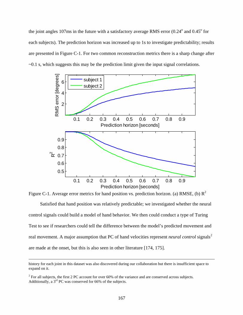
167

the joint angles 107ms in the future with a satisfactory average RMS error (0.24o and 0.45o for

each subjects). The prediction horizon was increased up to 1s to investigate predictability; results

are presented in Figure C-1. For two common reconstruction metrics there is a sharp change after

~0.1 s, which suggests this may be the prediction limit given the input signal correlations.

0.1 0.2 0.3 0.4 0.5 0.6 0.7 0.8 0.9

2

4

6

Prediction horizon [seconds]

RM

S e

rror [

degr

ees]

0.1 0.2 0.3 0.4 0.5 0.6 0.7 0.8 0.9

0.5

0.60.7

0.80.9

Prediction horizon [seconds]

R2

subject 1subject 2

Figure C-1. Average error metrics for hand position vs. prediction horizon. (a) RMSE, (b) R2

Satisfied that hand position was relatively predictable; we investigated whether the neural

control signals could build a model of hand behavior. We then could conduct a type of Turing

Test to see if researchers could tell the difference between the model’s predicted movement and

real movement. A major assumption that PC of hand velocities represent neural control signals2

are made at the onset, but this is also seen in other literature [174, 175].

history for each joint in this dataset was also discovered during our collaboration but there is insufficient space to expand on it.

2 For all subjects, the first 2 PC account for over 60% of the variance and are conserved across subjects. Additionally, a 3rd PC was conserved for 66% of the subjects.

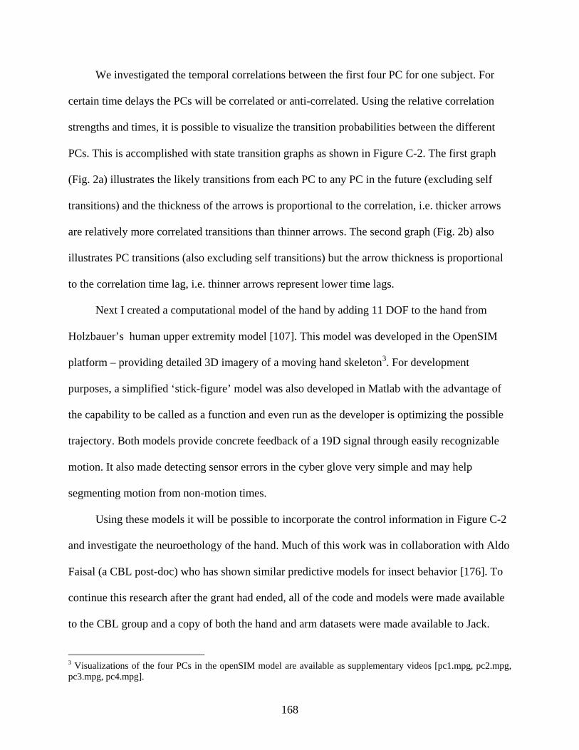
168

We investigated the temporal correlations between the first four PC for one subject. For

certain time delays the PCs will be correlated or anti-correlated. Using the relative correlation

strengths and times, it is possible to visualize the transition probabilities between the different

PCs. This is accomplished with state transition graphs as shown in Figure C-2. The first graph

(Fig. 2a) illustrates the likely transitions from each PC to any PC in the future (excluding self

transitions) and the thickness of the arrows is proportional to the correlation, i.e. thicker arrows

are relatively more correlated transitions than thinner arrows. The second graph (Fig. 2b) also

illustrates PC transitions (also excluding self transitions) but the arrow thickness is proportional

to the correlation time lag, i.e. thinner arrows represent lower time lags.

Next I created a computational model of the hand by adding 11 DOF to the hand from

Holzbauer’s human upper extremity model [107]. This model was developed in the OpenSIM

platform – providing detailed 3D imagery of a moving hand skeleton3. For development

purposes, a simplified ‘stick-figure’ model was also developed in Matlab with the advantage of

the capability to be called as a function and even run as the developer is optimizing the possible

trajectory. Both models provide concrete feedback of a 19D signal through easily recognizable

motion. It also made detecting sensor errors in the cyber glove very simple and may help

segmenting motion from non-motion times.

Using these models it will be possible to incorporate the control information in Figure C-2

and investigate the neuroethology of the hand. Much of this work was in collaboration with Aldo

Faisal (a CBL post-doc) who has shown similar predictive models for insect behavior [176]. To

continue this research after the grant had ended, all of the code and models were made available

to the CBL group and a copy of both the hand and arm datasets were made available to Jack.

3 Visualizations of the four PCs in the openSIM model are available as supplementary videos [pc1.mpg, pc2.mpg, pc3.mpg, pc4.mpg].

169

Figure C-2. State transition graphs for the first 4 PC of velocity. a) Thicker arrows represent

connections with higher correlations. b) Thinner arrows represent connections with faster maximum correlation lags. These graphs illustrate that the correlation between PC1 → PC2 has both the highest correlation value and the shortest lag. PC3 → PC2 is the weakly correlated with a long lag (note: PC3 and PC4 swaps in a) and b))

Broader Impacts of the International Cooperation

When I first arrived in Cambridge, I presented my current research to the CBL group [86]

to introduce myself. They were interested in the results but critical of the design because it was

unclear where the learning was occurring in the BMI model and the control task was relatively

unconstrained. There was an unexpected barrier between my engineering perspective and the

CBL group’s motor control theory perspective. However, the challenge was very helpful for me

to critically evaluate the role of paradigm design in BMI studies. Furthermore, it strengthened

my conviction that interdisciplinary work is a powerful way to solve problems but one must be

very cautious when drawing parallels to other fields.

170

After my original grant application, I continued research locally (at UF) for over one year

to acquire closed-loop BMI results prior to the trip. In this time we developed a novel BMI based

on Reinforcement Learning (RL). In this same time, Zoubin Ghahramani and Carl Rassmussen

continued to develop the machine learning group within the CBL to complement Dr. Wolpert’s

sensori-motor work. An unexpected benefit of the IREE grant was the exchange of ideas and

methods with the machine learning group. I gave a talk on the RL aspects of my research for that

group and received very specific and helpful feedback on the machine learning aspects. I also

helped with the RL tutorial day for the entire CBL that two of the machine learning graduate

students organized. Two of the students working on RL (or related) machine learning problems

are now very interested in BMI as an application. Many friendships were developed during this

stay and I have stayed in contact with people in CBL both on a personal and professional level.

The most striking cultural difference in the CBL group was the general work environment.

While my experience at UF has included working seven days a week when necessary, the CBL

group seemed much more efficient and capable of separating work and life. Also, there was

much more social interaction (e.g. a majority of the lab having lunch together) which led to more

collaboration. A concept that was strongly reinforced was that results should be fairly obvious;

data should not need to be processed within an inch of its life to illustrate a result. Their strong

focus on experimental design did allow the results to speak for themselves. Hypotheses were

addressed with simple metrics and generally did not need the processing power of the C-W.

The CBL also had a much higher ratio of post-docs to graduate students than our group at

UF. This was a unique experience to interact with some of the world’s leading authorities on

many different subjects. Instead of reading a paper to understand if an aspect of impendence

control would be useful for my work, I went to lunch with Dave Franklin and Luc Selen (two

171

post-docs advancing the state of the art in that area) to discuss it. Motor control is a broad topic

and the CBL is attacking the problem with unique but often complimentary approaches (with

little redundancy). This naturally creates a wonderful exchange of ideas.

There was also an unexpected benefit of learning from many different cultures in the CBL

group. The most culture exposure was obviously to the British from living in Cambridge and a

few weekend trips to London and Wales. However, the members of the CBL were from all over

the world including: New Zealand, Germany, Belgium, Iran, Canada, Holland, Japan, Italy,

Australia, and Turkey. Through our interactions and friendships, I was able to understand some

aspects of each culture

The supplement grant served to expand our initial grant by introducing new motor control

theories instead of focusing on movemes. It expanded the RL methods available to improve the

performance of our current RL-based BMI algorithm for the C-W. Also, it helped illustrate the

necessity of further refining paradigm design if we wanted to seriously address any neuroscience

questions. Finally, it helped develop our analysis of prior work to help get the work into a special

journal issue on Hybrid Bionics [86].

One area that I strived to improve was collaboration between engineering and motor

control theory. I tried to show the similarities in our goals and that we were not trying to overstep

our expertise into neuroscience but rather to use neuroscience concepts and synergistically

develop solutions to existing problems. Dr. Wolpert’s sensori-motor group was hesitant to

embrace was the field of adaptive filters (AF) commonly used in BMI. I started to bridge this gap

with AF predictors in the natural statistic hand dataset. Initially they suspected that simple curve

fitting or simple position/velocity models were sufficient. In Table C-1 the test set performance

of a WF is compared to other curve fitting techniques. Even with the advantage of testing on

172

training data, the curve fitting still had at least double the error. This convinced the CBL that AF

can exploit more complex spatio-temporal relationships in the data.

Table C-1. Performance of the hand PC predictor (LS) vs. a position + current velocity model.

Also shown are linear and quadratic curve fitting techniques. The error metrics are root-mean-squared, mean-squared, max error / range of signal, and coefficient of variation. The LS results are in the test set. The other fits were trained and tested on the training set.

Additionally, a sensitivity analysis [58] was performed to determine which input signals

were most useful for the predictors previously shown in Figure C-1. The sensitivity results for

one joint (representative) in both subjects and the pair-wise correlation analysis from [173] are

given in Figure C-3. The results are intuitive – the joints that are most correlated were the most

used by the AF. However, it lends credibility to this engineering approach (sensitivity analysis)

to Wolpert’s group who initially were skeptical.

Figure C-3. Sensitivity analysis for prediction of pinkie metacarpal-phalanges (p-mp) flexion

from the entire hand position. Shown on the left is a sensitivity analysis, besides the previous p-mp joint position the filter also uses ring, middle, index, and then thumb mp position. Shown on the right is the analysis from [173] of the percentage of variance that could be explained in the current pinkie position (labeled L) by pair-wise comparisons with other joint positions.

t-tm t-mp t-ij t-ab i-mp i-pi i-di m-mp m-pi m-di mi-ab r-mp r-pi r-di rm-ab p-mp p-pi p-di pr-ab0

0.1

0.2

0.3

0.4

0.5

0.6

0.7

0.8

0.9

1[t i m r p] = [thumb index middle ring pinkie] fingers

tm = trapezium-metacarpal joint

mp = metacarpal-phalanges joint

ip = inter-phalanges joint

ab = abduction

pi = proximal ip joint

di = distal ip joint

Mod

el S

ensi

tivity

Inputs from (t-250ms) to t

Predicitive Model of p-mp at (t+107ms) [red = subject 1, blue = subject 2]

173

Discussion and Summary

The datasets previously collected at the CBL were very interesting because it was

unconstrained and I believed it would facilitate investigation of an intrinsic aspect (i.e.

movemes) of the motor control system. Despite research finding movemes in a lab setting, the

null hypothesis is that the set of movemes [108] in ADL is unbounded. The financial and

technological investments necessary to force movemes into the C-W would be significant.

Understanding moveme utility was crucial before making such investments.

I was disappointed that the arm data set did not contain the necessary instrumentation to

complete the analysis. Additionally, the lack of constraints in the hand data proved incredibly

challenging to analyze. It was not possible to prove either the actual or null hypothesis because

both are prone to criticism. Lab experiments are less realistic and open to criticism that anything

extracted only reflect the paradigm biases. However, natural data requires investigators to create

rules determining when there is ‘movement’ otherwise roughly 75% of the data is resting. How

to create these rules elegantly is difficult because according to Dr. Selen, “motion starts when

you are born and ends when you die.” Having different subjects, tasks with unknown timescales,

and sensor noise only complicates the issue and create an opening for the criticism that say

anything extracted reflects the investigators biases. It seems a catch-22. This data segmentation

clearly affected all of the hand analysis we completed during the three month stay.

Despite these setbacks, we were still able to learn from the hand dataset both from

engineering and neuroethology perspectives. Specifically, we investigated relationships in

natural movement data on three different levels of abstraction. First, we considered the

interaction of the entire hand and did not employ any dimensionality reduction techniques. In

this investigation we found that the hand position could be predicted at 107 ms into the future

with less than 0.5 degrees average RMS error based on approximately 500 ms of hand position

174

history. Additionally, sensitivity analysis revealed that the filter’s prediction was most sensitive

to the most recent joint angle positions. Finally, certain joints were correlated with others (e.g.

ring finger with all other fingers) while others were only predicted by themselves (e.g. thumb).

The second level of investigation was into the hand control signals (again assuming PCs of

velocity reflect the neural control signals as in [174, 175]). We created a transitions map between

PCs including the overall transition likelihood and probable transition time based on the

correlations between different PCs. The maps can help develop a prior probability of control

signals; that type of information could be useful for a mixture-of-experts BMI. The maps are also

interesting from a neural perspective to understand the control strategies and cooperation. This

investigation was performed for one subject. Once the results can be better understood and

calculation techniques refined, it may be interesting to compare across subjects.

In order to use these maps, a computational skeletal model was refined in openSIM/ SIM

and developed in Matlab. Both of these models were given to the CBL for further use. These

computational models expose the transitions maps to an advanced critic – human eyes. However,

as maps and techniques are refined, we expect to advance the research as in [176].

The final level was to consider individual joints independently from the rest of the hand.4

In this investigation we found that each joint has a different time constant - a different amount of

embedded time history is necessary to form a state descriptor. These time constants were

variable across subjects and may be related to the average joint velocity. To quantify these

relationships will require more subjects and/ or improved performance metrics. However, even a

rough estimate was helpful to provide bounds on the amount of history included in other

correlation analysis.

4 The analysis was interesting but the variability between subjects was very high; it required multiple figure and detailed explanation. We regret it could not be explained in more detail due to space constraints.

175

The opportunity to live, learn, and work in another country for three months was incredibly

stimulating intellectually and broadened my perspectives. It forced me to re-examine my

preconceptions about other cultures and my own. Furthermore, it brought sharply into focus the

strengths and weakness of my own research; these details had been blurred because I knew my

entire project intimately. My main recommendation for the IREE program is to advertise it more

widely because many colleagues on NSF grants were unaware of this great opportunity until my

experience. One final suggestion is that the IREE program strongly recommends travel periods

of at least four months. It takes time to move to a new city, adjust to the new lab culture, and

begin to make contributions. This adjustment time may only be a week or two but that is still

substantial relative to a two or three month visit.

176

APPENDIX D INTERNATIONAL RESEARCH IN ENGINEERING AND EDUCATION REPORT:

SCUOLA SUPERIORE SANT’ANNA

Introduction

Brain-Machine Interface (BMI) is an active research topic with the potential to improve

the lives of individuals afflicted with motor neuropathies [9]. For the past eighteen years, the

Computational NeuroEngineering Laboratory (CNEL) at the University of Florida (UF) has been

pioneering the development of signal processing models used to translate neural activity into

behavior [164]. Our interdisciplinary group also includes the Neuroprosthetics Research Group

(NRG), and Advanced Computing and Information Systems (ACIS) Laboratory. We are

developing a Cyber-Workstation (C-W) to obliterate limitations currently faced by BMI

designers, i.e. the C-W provides tremendous remote computing power [165] yet still returns BMI

outputs (e.g. prosthetic commands) locally to satisfy real-time deadlines [137]. Furthermore the

C-W provides an integrated environment for efficient code development and repeatable analysis

of results [134, 135, 137]. This ground-breaking research is supported by the Dynamic Data

Driven Applications Systems (DDDAS) section of the National Science Foundation.

At the core of the C-W architecture is Wolpert and Kawato’s theory of motor control

which uses Multiple, Paired Forward and Inverse Models (MPFIM) [16]. MPFIM in an

intriguing theory that has been further refined but the idea of control via predictive modules has

remained intact [70, 166, 167]. The C-W is particularly suited to utilize MPFIM architecture

because the C-W exploits grid-computing to process the multiple sets of models in parallel.

Furthermore, it provides power and flexibility for BMI designers. Regardless of whether their

BMI incorporates MPFIM theory, the designer still has access to N (currently 10, but

expandable) sets of up to three interacting models in which he or she can place any algorithm.

177

A natural extension to our project was to broaden the impact by investigating different

prosthetics and robotic control strategies. In our BMI research (which can be rapidly processed

by the C-W), we have provided real-time feedback to the BMI user (a rat) by physically moving

a prosthetic (a robot arm) [86]. The robot is the MiniCRANE (Dynaservo, Markham ON) which

has five Degree Of Freedoms (DOF). The robot is both precise and fast and we can successfully

use inverse kinematics optimization to generate the necessary relative joint angle changes to

maneuver it and provide real-time feedback in a BMI [86]. However, the control we have

achieved may be unnatural for a BMI user and could degrade learning.

Jack DiGiovanna was sent to learn natural robot control strategies with Dr. Silvestro

Micera in the Advanced Robotics Technologies & Systems (ARTS) Lab (Scuola Superiore

Sant’Anna) from January to April of 2008. Jack was a natural candidate because he was

responsible for our current BMI robotic control scheme [86]. As a 3rd year biomedical

engineering graduate student, he was trained both as a BMI designer and behaviorist. In the

process of BMI design, he also interfaced directly with the robotic hardware; hence was the most

prepared student on our grant to start a dialogue with members of the ARTS lab.

Professor Paolo Dario’s ARTS lab is world renown for neuro-robotics systems [140].

Currently the ARTS lab is developing a bio-mechatronic tendon force sensor to provide feedback

for advanced control schemes. They are also developing task-specific robot devices that can

interface with a general control device to provide the greatest utility to the patient. Another

recent research area has been integrating their prosthetic devices more naturally with the

peripheral and central nervous systems. They have had success using EMG and other neural

signals as control inputs and using native nerve paths to provide feedback (other than visual) to

the patient. The ARTS lab uses a systems neurophysiology approach to create devices, i.e.

178

developing an artificial sensory system based on human physiology. This artificial sensory

system provides sufficient feedback to achieve accurate control.

Our motivation for collaborating with the ARTS lab is the robot component of our BMI

paradigm [86]. Other researchers have shown that incorporating more intelligence into the robot

and using a more biologically-based design can improve BMI performance [78-80]. The ARTS

lab’s unique expertise in this field and experience designing integrated biomimetic systems

would be incredibly helpful for this type of control improvement. Additionally, it is possible that

BMI users could learn control more rapidly if the interface feels more similar to their own motor

control system. The ARTS lab would benefit from access to CNEL’s advanced BMI algorithms,

signal processing, and ACIS’s grid-computing infrastructure. We offer a challenging and new

paradigm for the ARTS lab to further their research in neuro-robotics. Different perspectives

and use of the tools and ideas that we share would also encourage collaboration beyond the scope

and length of this grant.

Research Activities and Accomplishments of the International Cooperation

The ARTS lab is not only involved in robot design, but is also working extensively on

electrode for the Peripheral Nervous System; that was the research area where our collaboration

was most productive. Electrodes are critically important to BMI research; in fact electrodes are

currently a weak-link in developing robust, invasive BMI for clinical applications [8, 10, 50,

177]. The problem arises from neural signal sensing degradation which is the loss in signal

quality (decreasing SNR) over time in chronically implanted electrodes. This problem may stem

from the electrode moving with respect to the neuron, electrode degradation, and/or glial scarring

which encapsulates the electrode [9, 177]. BMI developers use the similar retraining approach to

overcome this issue periodically re-sorting and reclassifying responding spikes (for review see

[131]). The most current (possibly degraded) neural signals are re-sorted such that individual

179

neurons can be discriminated with new templates. Besides being time intensive and requiring

expert supervision [131], this approach ultimately cannot overcome the total loss of the neural

signal.

Longitudinal Intra Fascicular Electrodes (LIFE) have shown promising semi-chronic

stability and relatively minimal encapsulation and nerve damage in animal and human subjects

[177, 178]. LIFE penetrate the epineurum and perineum, are oriented approximately parallel to

the nerve fiber, and may have multiple recording sites. The issue of neural signal stability for

LIFE is investigated in a rabbit model. However, instead of looking at structural or physiological

changes, LIFE’s functional stability is inferred. Specifically, the following functional question

was addressed: Does electrode degradation and/or immune response to LIFE adversely affect

BMI performance? A standard technique (re-spike sorting each session) is compared against re-

using old sorts in a BMI. Re-sorting is mainly necessary to overcome neural signal sensing

degradation; it is shown to be unnecessary using LIFE implanted for over four months [125].

The single unit firing rates extracted from each LIFE (see [125] for more details) were

processed in a BMI to test the functional stability of LIFE. We assume re-sorting the ENG data

effectively overcomes neural signal degradation. Furthermore, we assume neural signal

degradation should adversely affect BMI performance. Therefore, we inferred the neural signal

degradation based on BMI performance with and without re-spike sorting, i.e. if performance is

significantly worse then the neural signal has been degraded. We also tested our assumption that

combining single units into a NND signal will create a more stable signal; hence, improve BMI

performance. We compared the NND inputs (all units averaged together) with neural

discriminated (ND) inputs (all units considered unique) for the BMI. We test one linear and one

non-linear BMI to construct the mapping between the NND or ND signals and ankle position.

180

The Wiener Filter (WF) was used for the linear BMI because it provides a reliable benchmark in

BMI research and an optimal linear mapping for the given input-output signals [145]. A single-

layer perceptron (SLP) with a hyperbolic tangent nonlinearity is used for the non-linear BMI

[145] to exploit a non-linear relationship between the input and ankle position. BMI performance

in all test segments was used to determine statistical significance.1 Average test segment

performance is reported.

All networks were evaluated using two common BMI performance metrics: mean squared

error (MSE) and maximum error. There were two electrodes per LIFE for each rabbit (four

electrodes total); however, one electrode had a mechanical connection problem and was

excluded from the analysis. All combinations of BMI type (WF or SLP), input type (NND or

ND), and template creation (re-sorted or static) were tested in this analysis (8 BMI per

electrode). The two electrodes from the same LIFE were not grouped together because BMI

performance (not reported) was not significantly better than using each electrode separately

First, we tested the assumption that NND input data can be used instead of ND. We

compared the performance in linear and non-linear BMIs with static templates (alternatively re-

sorted templates could have been used). Figure D-1 shows this comparison for a representative

LIFE. For all three LIFE, the SLP with NND input data provided significantly better

performance than any other BMI-input combination for both MSE and maximum error.

Additional tests showed significant differences in each BMI type’s performance with NND vs.

ND inputs. The WF with NND inputs performed significantly worse than a WF with ND inputs.

However, the SLP with NND inputs performed significantly better than a SLP with ND inputs.

The significance applied to both performance metrics. This performance discrepancy may be due

1 All reported significance is determined with 2-sample Kolmogorov-Smirnov tests at 95% confidence.

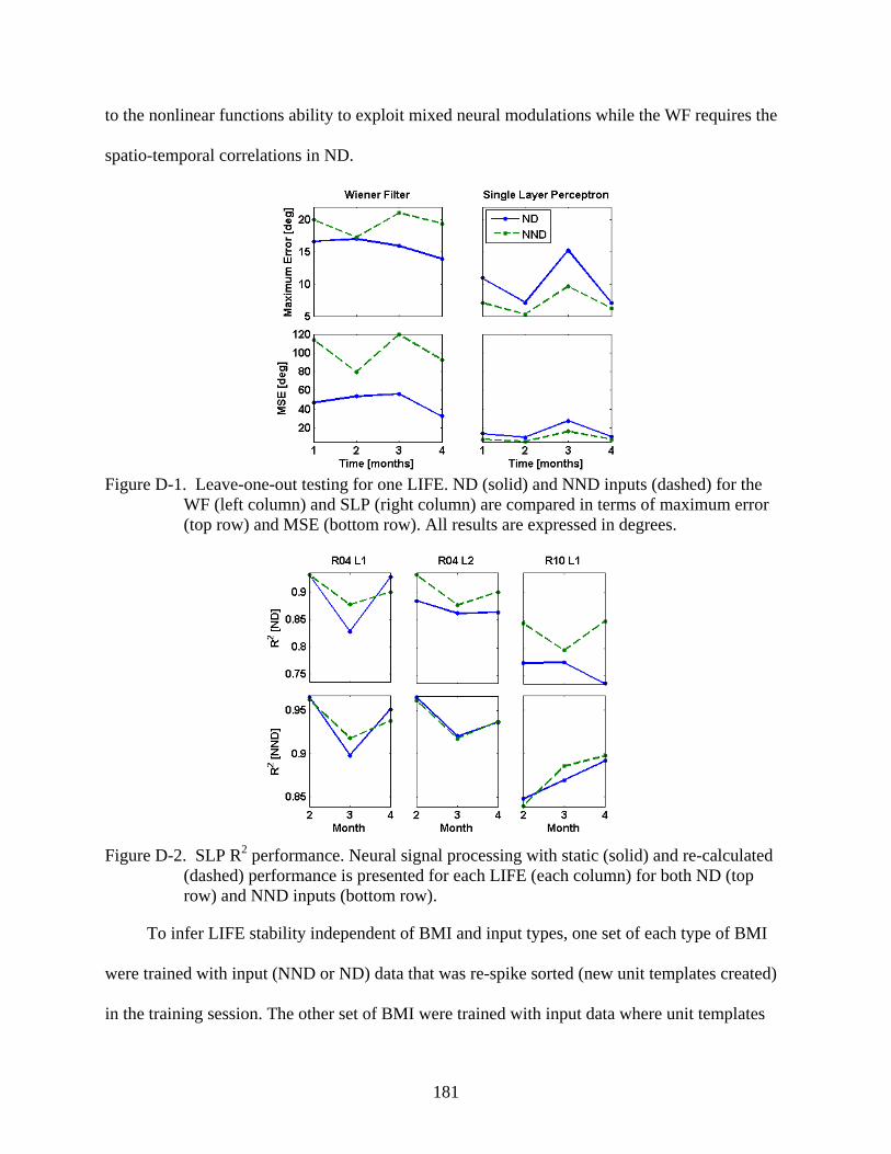
181

to the nonlinear functions ability to exploit mixed neural modulations while the WF requires the

spatio-temporal correlations in ND.

Figure D-1. Leave-one-out testing for one LIFE. ND (solid) and NND inputs (dashed) for the

WF (left column) and SLP (right column) are compared in terms of maximum error (top row) and MSE (bottom row). All results are expressed in degrees.

Figure D-2. SLP R2 performance. Neural signal processing with static (solid) and re-calculated (dashed) performance is presented for each LIFE (each column) for both ND (top row) and NND inputs (bottom row).

To infer LIFE stability independent of BMI and input types, one set of each type of BMI

were trained with input (NND or ND) data that was re-spike sorted (new unit templates created)

in the training session. The other set of BMI were trained with input data where unit templates

182

were created in the initial session and kept static. Figure D-2 compares the correlation coefficient

(R2) between SLP output and ankle position for ND and NND inputs. R2 was used to simplify the

figure but it is also a common BMI performance metric. For all three LIFE and all BMI-input

combinations (12 total comparisons) performance with static templates was not significantly

different than using re-sorted templates. The significance applied to both the MSE and maximum

error performance metrics and also the R2 metric. From this result we inferred that these LIFE

were functionally stable over four months of recording.

Broader Impacts of the International Cooperation

When I first arrived in Pontedera, I presented my current research to the ARTS lab [86] to

introduce myself. They were interested in the results and the learning mechanism controlling the

robot. I was also introduced to many different people at the lab who were working on all kinds of

robots. The hardware was amazingly life-like and the lab was bubbling with activity. One

surprising thing though was their interest in my work – despite the advance robotic technologies;

they still lacked a robust but efficient BMI control algorithm for the devices. I had thought that I

could learn better control strategies from the ARTS lab.

After my original grant application, I continued research locally (at UF) for over one year

to acquire closed-loop BMI results prior to the trip. In this time we developed a novel BMI based

on Reinforcement Learning (RL). Of course the ARTS lab was also continuing to grow and

refine technologies. Their Cyber-Hand [139, 140, 177] had gained wide media attention and is

now being commercialized; in my time at ARTS there was never more than 2 weeks between

film crews coming to report on the project.

The most striking cultural difference in the ARTS lab was the general work environment.

While my experience at UF has included working seven days a week when necessary, the ARTS

lab had much clearer separations of work and life. Generally there was much more research

183

entropy among students at the ARTS lab – based on some of the 1st year Ph.D. proposals it

seemed each student should earn at least two separate degrees because the research was in so

many different areas. Also, there was much more social interaction (e.g. large groups in the lab

having lunch together) which led to more collaboration. In fact, one day I when I was working

through lunch with my laptop, multiple lab-mates came to check that everything was alright and

I was not sick. The social interaction was pleasant, but actually lengthened the work day.

The ARTS lab had a higher ratio of post-docs to graduate students than our group at UF.

However, most of the post-docs were in an entirely different research area than me. Regardless,

there was still an interesting exchange of ideas. Also there were opportunities for student

interaction and it was very nice to be able to help and be helped by others with different topics.

There was also the obvious cultural difference between Italy and the United States.

Although the official language was English at the ARTS lab, most of the causal conversation was

in Italian. Also, Pontedera is a small town and English is not generally spoken. In order to eat, it

was necessary to speak Italian – this was an excellent and powerful motivator to engage me in

the culture and language. Members of the ARTS labs represented almost all of the different

regions of Italy; through our interactions and friendships, I was able to understand some aspects

of the cultures of each region.

The supplement grant served to expand our initial grant by introducing new signal

processing methods for extracting neural signals from electrodes. This is very interesting to our

group at NRG despite the difference in electrode technology. The electroneurographic (ENG)

signal has low SNR and we used wavelet de-noising (WD) with template-based spike sorting to

discriminate afferent signals [179]. Specifically we use the translation-invariant wavelet

transform [180] with discrete wavelet transforms (Symlet 7 mother wavelet) as in [179].

184

Potential single units in the de-noised signal were identified and discriminated with standard

template-matching based spike-sorting methods [181, 182].

The SLP results shown in Figure D-1 raise the question of whether spike sorting is

necessary at all in this experiment. We compare an SLP with all sections of de-noised signal

greater than three standard deviations marked as units vs. an SLP with sorted units (both

networks used NND). The performance was not significantly different for all LIFE in both

performance metrics. This result suggests that spike sorting after WD may be unnecessary when

using NND SLP and merits future investigation. Reducing the need for spike sorting or

improving discrimination ability would be immensely beneficial for all BMI.

As a result of this grant, we completed the research which is highlighted in this report and

was later presented at the 2008 IEEE International Conference on Engineering in Medicine &

Biology [125]. The presentation received positive feedback. The collaboration had direct benefits

for the ARTS lab, including the ability to learn RL-control concepts and learning about our

current RL-based BMI algorithm [86] for controlling their prosthetics.

In fact, the ARTS lab has included these RL concepts into a closed loop neuro-prosthetics

projects that has recently been approved (exact details are confidential). It is a major

international collaboration with universities in Italy, Germany, UK, Switzerland, and the USA

over the next four years. The RL-based BMI control concepts that I introduced to the lab are a

key component to the prosthetic design.

In terms of continued collaboration, Silvestro Micera has already discussed future work

with both the CNEL and NRG labs for BMI development and control. An ARTS lab student will

also probably visit UF to collaborate with Dr. Principe at CNEL in the next year. Finally,

Silvestro has offered a post-doc position for me to advance the RL-based BMI controller for the

185

neuro-prosthetic grant. Obviously through my strong connections with the CNEL, NRG, and

ACIS labs, this would create opportunities to continue and expand the international

collaboration.

Discussion and Summary

During our collaboration, we designed three experiments in chronic LIFE recordings from

a rabbit model. The first examined an assumption (based on the PESH) that all discriminated

units had the same functional response. NND inputs performed significantly better than ND

inputs for non-linear BMI. However, NND inputs performance significantly worse than ND

inputs for linear BMI. Figure D-1 showed that changing the input to the SLP produced a

correlated (R2 of NND and ND performance = 0.97) difference in performance, possibly due to

the reduced number of BMI parameters. However, the difference WF performance was not

correlated (R2 = 0.26), suggesting the WF exploited the spatio-temporal correlations in the ND to

find a better mapping to the ankle position. It also could mean that SLP training should be

improved to better learn correlations in ND data. However, multiple SLP were trained for each

test to avoid dependencies on initial conditions and the training parameters were optimized based

on cross-validation in a representative LIFE [145].

The second experiment was not an initial focus of our work but was added based on the

NND results from the first experiment – the question was whether spike sorting was necessary to

reconstruct ankle position. While it is certainly exciting to consider processing neural data

without spike sorting, there are potential confounds. It is possible that WD removes all noise in

neural signal. This requires that the power spectrum of external noise (including electromagnetic

and EMG) is outside of 700 – 6 kHz or the amplitude is less than ENG (1-10µV). Additionally,

all signals recorded on the electrode may be stretch receptors but certain candidates were not

186

marked as a template because of low firing rates. Hence, all recorded signals must be generated

from the same neural population for this to work. These are two strong assumptions that must be

carefully examined before discarding spike sorting. Finally, spike sorting and PESH can

discriminate functional groups of neurons which has been useful for BMI [104, 109].

The final experiment was designed to infer the functional stability of LIFE in this rabbit

model. We assumed that re-creating spike-sorting templates each session is only necessary to

counter-act neural signal degradation due to immune response and/ or electrode degradation. We

find that BMI performance is not significantly different for three different electrodes (in two

different rabbits) when templates were not re-sorted. We infer from this result that the LIFE were

functionally stable for the duration of this 4 month recording.

Although the BMI were only used for relative comparisons and not absolute performance,

it is important to note that the BMIs in this study had an advantage of mapping neural signal to

repeatable (over trials) signal. Typically an afferent-based BMI would require signals from

muscle agonist-antagonist pairs to map both flexion and extension of a joint. However, these

BMI exploited information in the gamma taps (time embedding) to predict the ankle position

during extension where neural activity was negligible (see [125] for more details). If extension

was not repeatable, the BMI reconstruction would suffer.

The opportunity to live, learn, and work in another country for three months was incredibly

stimulating intellectually and broadened my perspectives. It forced me to re-examine my

preconceptions about other cultures and my own. Furthermore, it brought sharply into focus the

strengths and weakness of my own research; these details had been blurred because I knew my

entire project intimately. Many friendships were developed during this stay and I have stayed in

contact with people in the ARTS lab both on a personal and professional level. My main

187

recommendation for the IREE program is to advertise it more widely because many colleagues

on NSF grants were unaware of this great opportunity until my experience. One final suggestion

is that the IREE program strongly recommends travel periods of at least four months. It takes

time to move to a new city, adjust to the new lab culture, and begin to make contributions. This

adjustment time may only be a week or two but that is still substantial relative to a two or three

month visit.

188

LIST OF REFERENCES

[1] National Spinal Cord Injury Statistical Center, "Spinal Cord: Facts and Figures at a Glance - June 2006," http://images.main.uab.edu/spinalcord/pdffiles/Facts06.pdf, 2006.

[2] American Stroke Association, "Impact of Stroke," http://www.strokeassociation.org, 2007.

[3] C. Gray, French, J., Bates, D., Cartilidge, N., James, O. and Venables, G., "Motor recovery following acute stroke," Age and Aging, vol. 19, pp. 179-184, 1990.

[4] M. Weisskopf, "A Grim Milestone: 500 Amputees," in Time, 2007.

[5] National Institute of Neurological Disorder and Stroke, "Amyotrophic Lateral Sclerosis Fact Sheet," http://www.ninds.nih.gov/disorders/amyotrophiclateralsclerosis/detail_amyotrophic lateralsclerosis.htm, 2006.

[6] National Institute of Neurological Disorder and Stroke, "Muscular Dystrophy: Hope through Research ", http://www.ninds.nih.gov/disorders/md/detail_md.htm 2007.

[7] G. Loeb, Davoodi, R, "The functional reanimation of paralyzed limbs," in IEEE EMBS Magazine. vol. 24, 2005, pp. 45-51.

[8] E. C. Leuthardt, G. Schalk, D. Moran, and J. G. Ojemann, "The emerging world of motor neuroprosthetics: A neurosurgical perspective," Neurosurgery, vol. 59, pp. 1-13, Jul 2006.

[9] J. C. Sanchez and J. C. Principe, Brain Machine Interface Engineering: Morgan and Claypool, 2007.

[10] A. Schwartz, Cui, XT, Weber, DJ, Moran, DW, "Brain-Controlled Interfaces: Movement Restoration with Neural Prosthetics," Neuron, vol. 52, pp. 205-220, 2006.

[11] N. Bernstein, The co-ordination and regulation of movements. Oxford, UK: Pergamon Press, 1967.

[12] E. Guigon, Baraduc, P, and Desmurget, M, "Computational motor control: redundancy and invarience," Journal of Neurophysiology, vol. 97, pp. 331-347, 2007.

[13] S. Goodman, Latash, ML, "Feed-forward control of a redundant motor system," Biol. Cybernetics, vol. 95, pp. 271-280, 2006.

[14] P. Bays, and Wolpert, DM, "Computational principles of sensorimotor control that minimise uncertainty and variability," Journal of Physiology, vol. Physiology in Press, 2006.

[15] P. Davidson, and Wolpert, DM, "Widespread access to predictive models in the motor system: a short review," Journal of Neural Engineering, vol. 2, pp. s313-s319, 2005.

[16] D. Wolpert, Kawato, M "Multiple paired forward inverse models for motor control," Neural Networks, vol. 11, pp. 1317-1329, 1998.

189

[17] J.-F. Yang, Scholz, JP, Latash, ML, "The role of kinematic redundancy in adaptation of reaching," Exp. Brain Research, vol. 176, pp. 54-69, 2007.

[18] M. Haruno, and Wolpert, DM, "Optimal control of redundant muscles in step-tracking wrist movements," Journal of Neurophysiology, vol. 94, pp. 4244-4255, 2005.

[19] E. Todorov, Ghahramani, Z, "Unsupervised learning of sensory-motor primitives," in IEEE EMBC, New Jersey, 2003, pp. 1750-1753.

[20] E. Todorov, "Optimality principles in sensorimotor control," Nat Neurosci, vol. 7, pp. 907-915, 2004.

[21] D. Liu and E. Todorov, "Evidence for the flexible sensorimotor strategies predicted by optimal feedback control," manuscript under review, 2006.

[22] E. Todorov, "Programmable sensorimotor transformations and optimality of mixed representations," Manuscript under review, 2006.

[23] J. B. Dingwell, C. D. Mah, and F. A. Mussa-Ivaldi, "Experimentally Confirmed Mathematical Model for Human Control of a Non-Rigid Object," Journal of Neurophysiology, vol. 91, pp. 1158-1170, 2004.

[24] M. Abeles, Corticonics: Neural Circuits of the Cerebral Cortex. New York: Cambridge University Press, 1991.

[25] A. Guyton, and Hall, JE, Textbook of medical physiology, 10th ed. Philadelphia: W. B. Saunders Company, 2001.

[26] K. Doya, "What are the computations of the cerebellum, the basal ganglia and the cerebral cortex," Neural Networks, vol. 12, pp. 961-974, 1999.

[27] S. H. Scott, "Inconvenient Truths about neural processing in primary motor cortex," J Physiol, vol. 586, pp. 1217-1224, March 1 2008.

[28] M. H. Monfils, E. J. Plautz, and J. A. Kleim, "In Search of the Motor Engram: Motor Map Plasticity as a Mechanism for Encoding Motor Experience," The Neuroscientist, vol. 11, pp. 471-483, October 1 2005.

[29] J. A. Kleim, S. Barbay, and R. J. Nudo, "Functional reorganization of the rat motor cortex following motor skill learning," J Neurophysiol, vol. 80, pp. 3321-3325., 1998.

[30] J. A. Kleim, T. M. Hogg, P. M. VandenBerg, N. R. Cooper, R. Bruneau, and M. Remple, "Cortical Synaptogenesis and Motor Map Reorganization Occur during Late, But Not Early, Phase of Motor Skill Learning," Journal of Neuroscience, vol. 24, pp. 628-633, January 21 2004.

[31] A. Georgopoulos, Langheim, FJ, Leuthold, AC, Merkle, AN, "Magnetoencephalographic signals predict movement trajectory in space," Exp. Brain Research, vol. 167, pp. 132-135, 2005.

190

[32] N. Weiskopf, Mathiak, K, Bock, SW, Schamowski, F, Veit, R,Grodd, W, Goebel, R, and Birbaumer, N, "Principles of a brain-computer interface (BCI) based on real-time functional magnetic resonance imaging (fMRI)," IEEE Trans. Biomed. Eng., vol. 51, pp. 966-970, 2004.

[33] S. Yoo, Fairneny, T, Chen, NK, Choo, SE, Panych, LP, Park, H, Lee, SY, Jolesz, FA, "Brain-computer interface using fMRI: Spatial navigation by thoughts," Neuroreport, vol. 15, pp. 1591-1595, 2004.

[34] A. Scwartz, Cui, XT, Weber, DJ, Moran, DW, "Brain-Controlled Interfaces: Movement Restoration with Neural Prosthetics," Neuron, vol. 52, pp. 205-220, 2006.

[35] W. Freeman, "State variables from local field potentials for brain-machine interface," Cognitive Neurodynamics [in press], 2006.

[36] J. Wolpaw, McFarland, DJ, "Control of a two-dimensional movement signal by a noninvasive brain-computer interface in humans," PNAS, pp. 17849-17854, 2004.

[37] G. Fabiani, McFarland, DJ, Wolpaw, JR, Pfurtscheller, G, "Conversion of EEG activity into cursor movement by a brain-computer interface (BCI)," IEEE Trans. on Rehabilitation Engineering, vol. 12, pp. 331-338, 2004.

[38] E. C. Leuthardt, K. J. Miller, G. Schalk, R. P. N. Rao, and J. G. Ojemann, "Electrocorticography-based brain computer interface - The Seattle experience," IEEE Trans. Neural Systems and Rehabilitation Engineering, vol. 14, pp. 194-198, Jun 2006.

[39] E. C. Leuthardt, G. Schalk, J. R. Wolpaw, J. G. Ojemann, and D. W. Moran, "A brain-computer interface using electrocorticographic signals in humans," Journal of Neural Engineering, vol. 1, pp. 63-71, 2004.

[40] J. Sanchez, Gunduz, A, Principe, JC, Carney, PR, "Extraction and Localization of Mesoscopic Motor Control Signals for Human ECoG Nueroprosthetics," Journal of Neuroscience Methods, vol. 167, pp. 63-81, 2008.

[41] P. Kennedy, Andreasen, D, Ehirim, P, King, B, Kirby, T, Mao, H, Moore, M, "Using human extra-cortical local field potentials to control a switch," Journal of Neural Engineering, vol. 1, pp. 72-77, 2004.

[42] J. Rickert, S. C. de Oliveira, E. Vaadia, A. Aertsen, S. Rotter, and C. Mehring, "Encoding of movement direction in different frequency ranges of motor cortical local field potentials," Journal of Neuroscience, vol. 25, pp. 8815-8824, Sep 2005.

[43] E. Fetz, "Real-time control of a robotic arm by neuronal ensembles," Nature Neuroscience, vol. 2, pp. 583-584, 1999.

[44] M. Nicolelis, "Actions from thoughts," Nature, vol. 409, pp. 403-407, 2000.

[45] P. Konig, P. Verschure, "Neurons in Action," Science, vol. 296, pp. 1817-1818, 2002.

191

[46] J. Donoghue, "Connecting cortex to machines: recent advandces in brain interfaces," Nature Neuroscience, vol. 5, pp. 1085-1088, 2002.

[47] J. Chapin, "Using multi-neuron population recordings for neural prosthetics," Nature Neuroscience, vol. 7, pp. 452-455, 2004.

[48] T. P. Trappenberg, Fundamentals of Computational Neuroscience. New York: Oxford University Press, 2002.

[49] J. Wessberg, C. R. Stambaugh, J. D. Kralik, P. D. Beck, M. Laubach, J. K. Chapin, J. Kim, S. J. Biggs, M. A. Srinivasan, and M. A. L. Nicolelis, "Real-time prediction of hand trajectory by ensembles of cortical neurons in primates," Nature, vol. 408, pp. 361-365, 2000.

[50] L. R. Hochberg, M. D. Serruya, G. M. Friehs, J. A. Mukand, M. Saleh, A. H. Caplan, A. Branner, D. Chen, R. D. Penn, and J. P. Donoghue, "Neuronal ensemble control of prosthetic devices by a human with tetraplegia," Nature, vol. 442, pp. 164-171, 2006.

[51] E. M. Schmidt, "Single neuron recording from motor cortex as a possible source of signals for control of external devices," Ann. Biomed. Eng., vol. 8, pp. 339-349, 1980.

[52] A. Georgopoulos, J. Kalaska, R. Caminiti, and J. Massey, "On the relations between the direction of two-dimensional arm movements and cell discharge in primate motor cortex," Journal of Neuroscience, vol. 2, pp. 1527-1537, 1982.

[53] A. P. Georgopoulos, A. B. Schwartz, and R. E. Kettner, "Neuronal population coding of movement direction," Science, vol. 233, pp. 1416-1419, Sep 26 1986.

[54] A. P. Georgopoulos, R. E. Kettner, and A. B. Schwartz, "Primate motor cortex and free arm movements to visual targets in three-dimensional space. Coding of the direction of movement by a neuronal population," The Journal of Neuroscience: the Official Journal of the Society for Neuroscience, vol. 8, pp. 2928-2937, 1988.

[55] A. P. Georgopoulos, J. T. Lurito, M. Petrides, A. B. Schwartz, and J. T. Massey, "Mental rotation of the neuronal population vector," Science, vol. 243, pp. 234-236, Jan 13 1989.

[56] J. K. Chapin, K. A. Moxon, R. S. Markowitz, and M. A. Nicolelis, "Real-time control of a robot arm using simultaneously recorded neurons in the motor cortex," Nature Neuroscience, vol. 2, pp. 664-670, July 1999.

[57] P. R. Kennedy, R. A. Bakay, M. M. Moore, K. Adams, and J. Goldwaithe, "Direct control of a computer from the human central nervous system," IEEE Transactions on Rehabilitation Engineering, vol. 8, pp. 198-202, June 2000.

[58] J. C. Sanchez, J. M. Carmena, M. A. Lebedev, M. A. L. Nicolelis, J. G. Harris, and J. C. Principe, "Ascertaining the importance of neurons to develop better brain machine interfaces," IEEE Transactions on Biomedical Engineering, vol. 61, pp. 943-953, 2003.

192

[59] J. M. Carmena, M. A. Lebedev, R. E. Crist, J. E. O'Doherty, D. M. Santucci, D. F. Dimitrov, P. G. Patil, C. S. Henriquez, and M. A. Nicolelis, "Learning to control a brain–machine interface for reaching and grasping by primates," PLoS Biology, vol. 1, pp. 1-16, 2003.

[60] S. P. Kim, J. C. Sanchez, D. Erdogmus, Y. N. Rao, J. C. Principe, and M. A. Nicolelis, "Divide-and-conquer approach for brain machine interfaces: nonlinear mixture of competitive linear models," Neural Networks, vol. 16, pp. 865-871, 2003.

[61] A. B. Schwartz, D. M. Taylor, and S. I. H. Tillery, "Extraction algorithms for cortical control of arm prosthetics," Current Opinion in Neurobiology, vol. 11, pp. 701-708, 2001.

[62] D. M. Taylor, S. I. H. Tillery, and A. B. Schwartz, "Direct cortical control of 3D neuroprosthetic devices," Science, vol. 296, pp. 1829-1832, 2002.

[63] S. I. Helms Tillery, D. M. Taylor, and A. B. Schwartz, "Training in cortical control of neuroprosthetic devices improves signal extraction from small neuronal ensembles," Reviews in the Neurosciences, vol. 14, pp. 107-119, 2003.

[64] D. Taylor, Schwartz, AB, "Using virtual reality to test the feasibility of controlling an upper limb FES system directly from multiunit activity in the motor cortex," in 6th Annual IFESS Conference Cleveland, OH, 2001.

[65] D. M. Taylor, S. I. Helms Tillery, and A. B. Schwartz, "Information conveyed through brain-control: Cursor versus robot," IEEE Trans. Neural Systems and Rehabilitation Engineering, vol. 11, pp. 195-199, 2003.

[66] M. D. Serruya, N. G. Hatsopoulos, L. Paninski, M. R. Fellows, and J. P. Donoghue, "Brain-machine interface: Instant neural control of a movement signal," Nature, vol. 416, pp. 141-142, 2002.

[67] K. V. Shenoy, D. Meeker, S. Cao, S. A. Kureshi, B. Pesaran, C. A. Buneo, A. P. Batista, P. P. Mitra, J. W. Burdick, and R. A. Andersen, "Neural prosthetic control signals from plan activity," NeuroReport, vol. 14, pp. 591-597, 2003.

[68] S. Musallam, Corneil, BD, Greger, B, Scherberger, H, Anderson, RA, "Cognitive control signals for neural prosthetics," Science, vol. 305, pp. 258-262, 2004.

[69] H. Miyamoto, Morimoto, J, Doya, K, Kawato, M, "Reinforcement learning with via-point representation," Neural Networks, vol. 17, pp. 299-305, 2004.

[70] K. Doya, Samejima, K, Katagiri, K, and Kawato, M., "Multiple model-based reinforcement learning," Neural Computation, vol. 14, pp. 1347-1369, 2002.

[71] E. Todorov, W. Li, and X. Pan, "From task parameters to motor synergies: A hierarchical framework for approximately optimal control of redundant manipulators " J. Robot. Syst., vol. 22, pp. 691-710, 2005

193

[72] B. P. Olson, J. Si, J. Hu, and J. P. He, "Closed-loop cortical control of direction using support vector machines," IEEE Trans. on Rehabilitation Engineering, vol. 13, pp. 72-80, 2005.

[73] J. Hu, Si, J, Olson, B, He, J, "Feature detections in motor cortical spikes by principal components analysis," IEEE Trans. on Rehabilitation Engineering, vol. 13, pp. 256-262, 2005.

[74] B. Olson, He, JP, Hu, J, Si, J, "A conceptual brain machine interface system," in International Conference on Neural Interface and Control Wuhan, China, 2005.

[75] S. Haykin, Adaptive Filter Theory: Prentice Hall, 2002.

[76] G. Gage, Ludwig, KA, Otto, KJ, Ionides, EL, Kipke, DR, "Naive coadaptive cortical control," Journal of Neural Engineering, vol. 2, pp. 52-63, 2005.

[77] S. P. Kim, J. C. Sanchez, Y. N. Rao, D. Erdogmus, J. C. Principe, J. M. Carmena, M. A. Lebedev, and M. A. L. Nicolelis, "A Comparison of Optimal MIMO Linear and Nonlinear Models for Brain-Machine Interfaces," J. Neural Engineering, vol. 3, pp. 145-161, 2006.

[78] H. Kim, Biggs, SJ, Schloerb, DW, Carmena, JM, Lebedev, MA, Nicolelis, MAL, Srinivasan, MA, "Continuous shared control for stabilizing reaching and grasping with brain-machine interfaces," IEEE Trans. Biomed. Eng., vol. 53, pp. 1164-1172, 2006.

[79] S. Chan, Moran, DW, "Computational model of a primate arm: from hand position to joint angles, joint torques and muscle forces," Journal of Neural Engineering, vol. 3, pp. 327-337, 2006.

[80] H. Kim, J. Carmena, S. Biggs, T. Hanson, M. Nicolelis, and M. Srinivasan, "The muscle activation method: an approach to impedance control of brain-machine interfaces through a musculoskelatal model of the arm," submitted to IEEE Trans. Biomed. Eng., 2006.

[81] J. T. Francis and J. K. Chapin, "Neural ensemble activity from multiple brain regions predicts kinematic and dynamic variables in a multiple force field reaching task," Ieee Transactions on Neural Systems and Rehabilitation Engineering, vol. 14, pp. 172-174, Jun 2006.

[82] E. Todorov, "Direct cortical control of muscle activation in voluntary arm movements: a model," Nat Neurosci, vol. 3, pp. 391-398, 2000.

[83] J. F. Kalaska, S. H. Scott, P. Cisek, and L. E. Sergio, "Cortical control of reaching movements," Current Opinion in Neurobiology, vol. 7, pp. 849-859, 1997.

[84] S. H. Scott and J. F. Kalaska, "Changes in motor cortex activity during reaching movements with similar hand paths but different arm postures," Journal of Neurophysiology, vol. 73, pp. 2563-2567, Jun 1995.

[85] R. Shadmehr and S. P. Wise, The computational neurobiology of reaching and pointing: a foundation for motor learning. Cambridge, MA: The MIT Press, 2005.

194

[86] J. DiGiovanna, B. Mahmoudi, J. Fortes, J. C. Principe, and J. C. Sanchez, "Co-adaptive Brain-Machine Interface via Reinforcement Learning," IEEE Transactions on Biomedical Engineering, in press, 2008.

[87] J. Sanchez, Gunduz, A, Principe, JC, Carney, PR, "Extraction and Localization of Mesoscopic Motor Control Signals for Human ECoG Nueroprosthetics," submitted to Journal of Neuroscience Methods, 2007.

[88] W. J. Freeman, "Origin, structure, and role of background EEG activity. Part 3. Neural frame classification," Clin. Neurophysiol, vol. 116, pp. 1118-1129, 2005.

[89] M. A. L. Nicolelis, D. Dimitrov, J. M. Carmena, R. Crist, G. Lehew, J. D. Kralik, and S. P. Wise, "Chronic, multi-site, multi-electrode recordings in macaque monkeys," Proc. Natl. Acad. Sci. U.S.A., vol. 100, pp. 11041-11046, 2003.

[90] F. Rieke, D. Warland, R. de Ruyter van Stevenick, and W. Bialek, Spikes: Exploring the Neural Code. Cambridge, MA, USA: MIT Press, 1999.

[91] S. Haykin, Neural networks: a comprehensive foundation. New York: Toronto: Macmillan; Maxwell Macmillan Canada, 1994.

[92] C. M. Bishop, Neural networks for pattern recognition. Oxford: Oxford University Press, 1995.

[93] G. Buzsáki, Rhythms of the Brain. New York: Oxford University Press, 2006.

[94] E. N. Brown, R. E. Kass, and P. P. Mitra, "Multiple Neural Spike Train Data Analysis: State-of-the-art and Future Challenges," Nature Neuroscience, vol. 7, pp. 456-461, 2004.

[95] S. H. Scott, "Neuroscience: Converting thoughts into action," Nature, vol. 442, p. 141, 2006.

[96] National Science Foundation, "Future Challenges for the Science and Engineering of Learning," http://cnl.salk.edu/Media/NSFWorkshopReport.v4.pdf, 2007.

[97] T. W. Berger, J. K. Chapin, G. A. Gerhardt, D. J. McFarland, J. C. Principe, W. V. Soussou, D. Taylor, and P. A. Tresco, "International assessment of research and development in brain-computer interfaces," World Technology Evaluation Center, Baltimore, MD 2007.

[98] G. J. Gage, K. A. Ludwig, K. J. Otto, E. L. Ionides, and D. R. Kipke, "Naive coadaptive cortical control," Journal of Neural Engineering, vol. 2, pp. 52-63, 2005.

[99] S. I. H. Tillery, D. M. Taylor, and A. B. Schwartz, "Training in cortical control of neuroprosthetic devices improves signal extraction from small neuronal ensembles," Reviews in the Neurosciences, vol. 14, pp. 107-119, 2003.

[100] J. del R. Millan, "Adaptive brain interfaces," Comm of the ACM, vol. 46, pp. 75-80, 2003.

195

[101] J. R. M. Wolpaw, D.J.; Vaughan, T.M., "Brain-computer interface research at the Wadsworth Center," Rehabilitation Engineering, IEEE Transactions on vol. 8, pp. 222-226, 2000.

[102] R. S. Sutton, "Learning to predict by the methods of temporal differences," Machine Learning, vol. 3, pp. 9-44, 1988.

[103] R. S. Sutton and A. G. Barto, Reinforcement learning: an introduction. Cambridge: MIT Press, 1998.

[104] J. DiGiovanna, J. C. Sanchez, and J. C. Principe, "Improved Linear BMI Systems via Population Averaging," in International Conference of the IEEE EMBS, New York, 2006.

[105] V. Mountcastle, "The columnar organization of the neocortex," Brain, vol. 120, pp. 702-722, 1997.

[106] J. C. Horton and D. L. Adams, "The cortical column: a structure without a function," Philos Trans R Soc Lond B Biol Sci., vol. 360, pp. 837-862, 2005.

[107] K. Holzbaur, Murray, W, Delp, S, "A model of the upper extremity for simulating musculoskeletal surgery and analyzing neuromuscular control," Annals of Biomedical Eng, vol. 33, pp. 829-840, 2005.

[108] J. DiGiovanna, J. Sanchez, B. Fregly, and J. Principe, "Arm Motion Reconstruction via Feature Clustering in Joint Angle Space," in IEEE International Joint Conference on Neural Networks Vancouver, 2006.

[109] J. C. Sanchez, J. C. Principe, and P. R. Carney, "Is Neuron Discrimination Preprocessing Necessary for Linear and Nonlinear Brain Machine Interface Models," in 11th International Conference on Human-Computer Interaction, Las Vegas, Nevada, 2005.

[110] M. Nagurka, Yen, V, "Fourier-based optimal control of nonlinear dynamic systems," J. Dynamic Systems, Measurement, and Control, vol. 112, pp. 17-26, 1990.

[111] A. Erdemir, McLean, S, Herzog, W, and van den Bogert, AJ, "Model-based estimation of muscle forces exerted during movements," Clinical Biomechanics, vol. 22, pp. 131-154, 2007.

[112] Y. Uno, Kawato, M, and Suzuki, R, "Formation and control of optimal trajectory in human arm movement - minimum torque-change model," Biological Cybernetics, vol. 61, pp. 89-101, 1989.

[113] Y. Wada, Kaneko, Y, Nakano, E, Osu, R, and Kawato, M, "Quantitative examination for multi joint arm trajectory planning - using a robust calculation algorithm of the minimum commanded torque change model," Neural Networks, vol. 14, pp. 381-393, 2001.

[114] S. L. Delp and J. P. Loan, "A graphics-based software system to develop and analyze models of musculoskeletal structures," Comput. Biol. Med, vol. 25, pp. 21-34, 1995.

196

[115] A. van den Bogert, Gerritsen, KGM, and Cole, GK, "Human muscle modeling from a user’s perspective," J. Electromyography and Kinesiology, vol. 8, pp. 119-124, 1998.

[116] F. Worgotter and B. Porr, "Temporal sequence learning, prediction, and control: a review of different models and their relation to biological mechanisms," Neural Computation, vol. 17, pp. 245-319, 2005.

[117] R. S. Sutton, "Implementation details of the TD(λ) procedure for the case of vector predictions and backpropagation," 1989.

[118] J. Peters, Vijayakumar, S, Schaal, S, "Reinforcement learning for humanoid robotics," in IEEE-RAS Int. Conf. on Humanoid Robotics Karlsruhe, Germany, 2003.

[119] G. H. Bower, Theories of Learning, 5th ed. Englewood Cliffs: Prentice-Hall, Inc., 1981.

[120] J. DiGiovanna, B. Mahmoudi, J. Mitzelfelt, J. C. Sanchez, and J. C. Principe, "Brain-machine interface control via reinforcement learning," in IEEE EMBS Conference on Neural Engineering Kohala Coast, 2007.

[121] I. Q. Whishaw, The behavior of the laboratory rat. New York: Oxford University Press, Inc. , 2005.

[122] J. C. Principe, B. De Vries, and P. G. Oliveira, "The gamma filter - a new class of adaptive IIR filters with restricted feedback," IEEE Trans. Signal Processing, vol. 41, pp. 649-656, 1993.

[123] S. B. U. Maulik, "Performance evaluation of some clustering algorithms and validity indices," IEEE Trans. Pattern Analysis Machine Intelligence, vol. 24, December 2002.

[124] J. C. Sanchez, "From Cortical Neural Spike Trains to Behavior: Modeling and Analysis," in Department of Biomedical Engineering Gainesville: University of Florida, 2004.

[125] J. DiGiovanna, L. Citi, K. Yoshida, J. Carpaneto, J. C. Principe, J. C. Sanchez, and S. Micera, "Inferring the Stability of LIFE through Brain-Machine Interfaces," in International Conference of the IEEE EMBS Vancouver, 2008.

[126] E. Patrick, M. Ordonez, N. Alba, J. C. Sanchez, and T. Nishida, "Design and Fabrication of a Flexible Substrate Microelectrode Array for Brain Machine Interfaces," in IEEE International Conference of the Engineering in Medicine and Biology Society, New York, 2006.

[127] J. C. Sanchez, N. Alba, T. Nishida, C. Batich, and P. R. Carney, "Structural modifications in chronic microwire electrodes for cortical neuroprosthetics: a case study," IEEE Transactions on Neural Systems and Rehabilitation Engineering, vol. 14, pp. 217-221, 2006.

[128] R. Bashirullah, J. G. Harris, J. C. Sanchez, T. Nishida, and J. C. Principe, "Florida Wireless Implantable Recording Electrodes (FWIRE) for Brain Machine Interfaces," in Circuits and Systems, 2007. ISCAS 2007. IEEE International Symposium on, 2007, pp. 2084-2087.

197

[129] I. Q. Whishaw, B. Gorny, A. Foroud, and J. A. Kleim, "Long-Evans and Sprague-Dawley rats have similar skilled reaching success and limb representations in motor cortex but different movements: some cautionary insights into the selection of rat strains for neurobiological motor research," Behavioural Brain Research, vol. 145, pp. 221-232, 2003.

[130] J. P. Donoghue and S. P. Wise, "The motor cortex of the rat: cytoarchitecture and microstimulation mapping," J. Comp. Neurol., vol. 212, pp. 76-88, 1982.

[131] M. S. Lewicki, "A review of methods for spike sorting: the detection and classification of neural action potentials," Network: Computation in Neural Systems, vol. 9, 1998.

[132] G. Buzsaki and A. Kandel, "Somadendritic backpropagation of action potentials in cortical pyramidal cells of the awake rat,," Journal of Neurophysiology, vol. 79, pp. 1587-1591, 1998.

[133] J. J. Craig, Introduction to Robotics: Mechanics and Control, 2nd ed. Reading: Addison-Wesley Publishing Co., Inc., 1989.

[134] J. DiGiovanna, L. Marchal, P. Rattanatamrong, M. Zhao, S. Darmanjian, B. Mahmoudi, J. Sanchez, J. Príncipe, L. Hermer-Vazquez, R. Figueiredo, and J. Fortes, "Towards Real-Time Distributed Signal Modeling for Brain Machine Interfaces," in International Conference on Computational Science, 2007.

[135] R. F. J. Fortes, L. Hermer-Vazquez, J. Principe, and J. Sanchez, "A New Architecture for Deriving Dynamic Brain-Machine Interfaces," in International Conference on Computer Science, 2006.

[136] S. Blakeslee, "Monkey's Thoughts Propel Robot, a Step That May Help Humans," in New York Times, 2008.

[137] M. Zhao, P. Rattanatamrong, J. DiGiovanna, B. Mahmoudi, R. Figueiredo, J. C. Sanchez, J. C. Principe, and J. Fortes, "BMI Cyberworkstation: Enabling Dynamic Data-Driven Brain-Machine Interface Research Through Cyberinfrastructure," in IEEE Engineering in Medicine & Biology Vancouver, 2008.

[138] D. H. Wolpert and W. G. Macready, "No free lunch theorems for optimization," Evolutionary Computation, IEEE Transactions on, vol. 1, pp. 67-82, 1997.

[139] L. Citi, J. Carpaneto, K. Yoshida, K. P. Hoffmann, K. P. Koch, P. Dario, and S. Micera, "Characterization of tfLIFE Neural Response for the Control of a Cybernetic Hand," in BioROB, 2006.

[140] S. Micera, M. C. Carrozza, L. Beccai, F. Vecchi, and P. Dario, "Hybrid bionic systems for the replacement of hand function," Proceedings of the IEEE, vol. 94, pp. 1752-1763, 2006.

[141] M. P. Deisenroth, J. Peters, and C. E. Rasmussen, "Approximate Dynamic Programming with Gaussian Processes," in American Control Conference Seattle, 2008.

198

[142] F. Doshi, J. Pineau, and N. Roy, "Reinforcement learning with limited reinforcement: using Bayes risk for active learning in POMDPs," in Proceedings of the 25th international conference on Machine learning Helsinki, Finland: ACM, 2008.

[143] J. Si and Y.-T. Wang, "On-line learning control by association and reinforcement," IEEE Transaction on Neural Networks, vol. 12, pp. 264-276, 2001.

[144] W. C. Lefebvre, J. C. Principe, C. Fancourt, N. R. Euliano, G. Lynn, G. Geniesse, M. Allen, D. Samson, D. Wooten, and J. Gerstenberger, "NeuroSolutions," 4.20 ed Gainesville: NeuroDimension, Inc., 1994.

[145] S. Haykin, Adaptive filter theory, 3rd ed. Upper Saddle River, NJ: Prentice-Hall International, 1996.

[146] R. J. Williams, "Simple Statistical Gradient-Following Algorithms for Connectionist Reinforcement Learning," Machine Learning, vol. 8, pp. 229-256, 1992.

[147] C. Ojakangas, A. Shaikhounim, G. Friehs, A. Caplan, M. Serruya, M. Saleh, D. Morris, and J. Donoghue, "Decoding movement intent from human premotor cortex neurons for neural prosthetic applications," Journal of Clinical Neurophysiology, vol. 23, pp. 577-584, 2006.

[148] M. Spalding, et al., "abstract," in Society for Neuroscience, 2004-2005.

[149] M. Velliste, S. Perel, M. C. Spalding, A. S. Whitford, and A. B. Schwartz, "Cortical control of a prosthetic arm for self-feeding," Nature, vol. 453, pp. 1098-1101, 2008.

[150] B. Mahmoudi, J. DiGiovanna, J. C. Principe, and J. C. Sanchez, "Neural Tuning in a Reinforcement Learning-Based Brain Machine Interface," in IEEE EMBC 2008 Vancouver, 2008.

[151] A. C. Davison and D. Hinkley, "The Basic Bootstraps," in Bootstrap Methods and Their Application, 1st ed Cambridge: Cambridge University Press, 1997.

[152] J. A. Kleim, "Motor Control I: Pyramidal System," University of Florida, 2006.

[153] C. T. Moritz, S. I. Perlmutter, and E. E. Fetz, "Direct control of paralysed muscles by cortical neurons," Nature, 2008.

[154] S. Suner, M. R. Fellows, C. Vargas-Irwin, K. Nakata, and J. P. Donoghue, "Reliability of signals from a chronically implanted, silicon-based electrode array in non-human primate primary motor cortex," IEEE Trans. Biomed. Eng., 2004.

[155] C. E. Bonferroni, "Il calcolo delle assicurazioni su gruppi di teste," in Studi in Onore del Professore Salvatore Ortu Carboni Rome, 1935, pp. 13-60.

[156] E. W. Weisstein, "Bonferroni Correction from MathWorld." vol. 2008: Wolfram Research, Inc., 2008.

199

[157] J. Berger, Statistical Decision Theory and Bayesian Analysis. Berlin: Springer-Verlag, 1985.

[158] J. Marcum, "A statistical theory of target detection by pulsed radar," Information Theory, IRE Transactions on, vol. 6, pp. 59-267, 1960.

[159] D. C. McFarlane and K. Glover, Robust Controller Design Using Normalized Coprime Factor Plant Descriptions, 1st ed. New York: Springer, 1989.

[160] D. Heeger, "Signal Detection Theory." vol. 2008 New York: Department of Psychology, New York University, 2007.

[161] R. Jenssen, J. C. Principe, and T. Eltoft, "Cauchy-Schwartz pdf Divergence Measure for non-Parametric Clustering," in IEEE Norway Section Int'l. Symposium on Signal Processing (NORSIG2003), Bergen, Norway, 2003.

[162] N. D. Daw and K. Doya, "The computational neurobiology of learning and reward," Current Opinion in Neurobiology, vol. 16, pp. 199-204, 2006.

[163] J.-Y. Chang, J. Paris, S. Sawyer, A. Kirillov, and D. Woodward, "Neuronal spike activity in rat nucleus accumbens during cocaine self-administration under different fixed-ration schedules," Neuroscience, vol. 74, pp. 483-497, 1996.

[164] T. G. Chang, J. R. Smith, and J. C. Principe, "A knowledge-based system for the automated on line classification of EEG/EOG signals," Journal of Microcomputer Applications, vol. 10, pp. 54-65, 1990.

[165] V. C. Sumalatha Adabala, Puneet Chawla, Renato Figueiredo, José A. B. Fortes, Ivan Krsul, Andrea Matsunaga, Mauricio Tsugawa, Jian Zhang, Ming Zhao, Liping Zhu, Xiaomin Zhu, "From Virtualized Resources to Virtual Computing Grids: The In-VIGO System," Future Generation Computing Systems, 2005.

[166] H. Imamizu, Kuroda, T, Miyauchi, S, Yoshioka, T, & Kawato, M, "Modular organization of internal models of tools in the human cerebellum," PNAS, vol. 100, pp. 5461-5466, 2003.

[167] M. Kawato, Kuroda, T, Imamizu, H, Nakano, E, Miyauchi, S, and and T. Yoshioka, "Internal forward models in the cerebellum:fMRI study on grip force and load force coupling," Progress in Brain Research, vol. 142, pp. 171-188, 2003.

[168] K. Thoroughman, Shadmehr, R, " Learning of action through adaptive combinations of motor primitives," Nature, vol. 407, pp. 742-747, 2000.

[169] E. Hwang, Shadmehr, R, "Internal models of limb dynamics and the encoding of limb state," Journal of Neural Engineering, vol. 2, pp. s266-s278, 2005.

[170] A. d'Avella, Saltiel, P, and Bizzi, E, "Combinations of muscle synergies in the construction of a natural motor behavior," Nature Neuroscience, vol. 6, pp. 300-309, 2003.

200

[171] F. Mussa-Ivaldi, and Bizzi, E, "Motor learning through the combination of primatives," Phil. Trans. R. Soc. Lond. B, vol. 355, pp. 1755-1769, 2000.

[172] C. Padoa-Schioppa, Li, C-SR, and Bizzi, E, "Neuronal correlates of kinematics-to-dynamics transformation in the supplementary motor area," Neuron, vol. 36, pp. 751-765, 2002.

[173] J. N. Ingram, K. P. Kording, I. S. Howard, and D. M. Wolpert, "The statistics of natural hand movements," under review, 2008.

[174] L. A. Jones and S. J. Lederman, Human Hand Function: Oxford University Press, 2006.

[175] M. H. Schieber and M. Santello, "Hand function: peripheral and central constraints on performance," J Appl Physiol, vol. 96, pp. 2293-2300, June 1 2004.

[176] A. A. Faisal, J. E. Niven, and S. Rodgers, "Analysis of Decision Making in an Insect's Gap Crossing Behavior Using Markov Models," in Cosyne, 2008.

[177] X. Navarro, T. B. Krueger, N. Lago, S. Micera, T. Stieglitz, and P. Dario, "A critical review of interfaces with the peripheral nervous system for the control of neuroprostheses and hybrid bionic systems," Journal of the Peripheral Nervous System, vol. 10, pp. 229-258, 2006.

[178] N. Lago, K. Yoshida, K. P. Koch, and X. Navarro, "Assesment of Biocompatibility of Chronically Implated Polyimide and Platinum Intrafascicular Electrodes," IEEE Trans. Biomed. Eng., vol. 54, pp. 281-291, 2007.

[179] L. Citi, J. Carpaneto, K. Yoshida, K.-P. Hoffmann, K. P. Koch, P. Dario, and S. Micera, "On the use of wavelet denoising and spike sorting techniques to process ENG signals recorded using intra-neural electrodes," Journal of Neuroscience Methods, 2008.

[180] R. R. Coifman and D. L. Donoho, "Translation-invariant de-noising," in Wavelets and Statistics: Springer Verlag, 1995, pp. 125-150.

[181] A. Diedrich, W. Charoensuk, R. K. Brychta, A. C. Ertl, and R. Shiavi, "Analysis of raw microneurographic recordings based on wavelet de-noising technique and classification algorithm: Wavelet analysis in microneurography," IEEE Trans. Biomed. Eng., vol. 50, 2003.

[182] K. Yoshida and R. B. Stein, "Characterization of signals and noise rejection with bipolar longitudinal intrafascicular electrodes," IEEE Trans. Biomed. Eng., vol. 46, pp. 226-235, 1999.

201

BIOGRAPHICAL SKETCH

John (Jack) F. DiGiovanna earned a M.E. in biomedical engineering from the University of

Florida, Gainesville, in 2007 and is working to complete a PhD. He earned a B.S. in electrical

engineering (minor in bioengineering) from Penn State University, University Park, in 2002. He

joined the CNEL lab in 2004 and NRG lab in 2006. Jack’s research area is reinforcement

learning based brain-machine interface (BMI) and motor control systems. In 2007 he received an

NSF International Research in Engineering and Education grant and worked with the Sensory

Motor Control Group (Cambridge University) and the Advanced Robotics Technologies &

Systems Lab (Scuola Superiore Sant’Anna). He was a founding officer in the Gainesville IEEE

EMBS chapter. He holds one patent in neuroprosthetic design and is the author over 10 peer

reviewed papers.