Embed Size (px)
Citation preview
Will E. Leland, Walter Willinger and Daniel V. Wilson BELLCOREMurad S. Taqqu Boston University
CS634 ADVANCED COMPUTER NETWORKING
COMPUTER SCIENCE
COLLEGE OF WILLIAM AND MARY
ON THE SELF-SIMILAR NATURE OF
ETHERNET TRAFFIC
Presented by: Feng Yan

OVERVIEW
What is Self Similarity?
Ethernet Traffic is Self-Similar
Implications of Self Similarity
Conclusion
Discussion2

PART 1:
WHAT IS SELF-SIMILARITY ?

INTUITION OF SELF-SIMILARITY
Something “feels the same” regardless of scale
4What is that???

INTUITION OF SELF-SIMILARITY
Something “feels the same” regardless of scale
5
Self-similar in nature

INTUITION OF SELF-SIMILARITY
Something “feels the same” regardless of scale
6
The Koch snowflake fractal
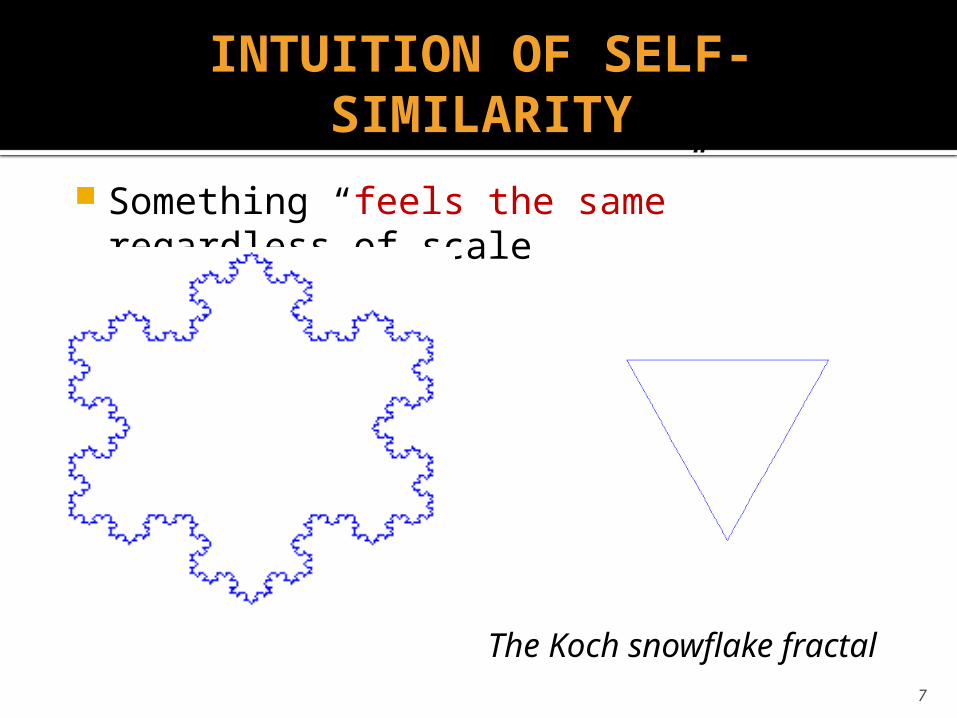
INTUITION OF SELF-SIMILARITY
Something “feels the same” regardless of scale
7
The Koch snowflake fractal
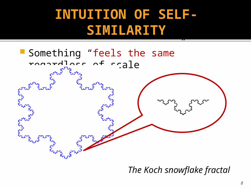
INTUITION OF SELF-SIMILARITY
Something “feels the same” regardless of scale
8
The Koch snowflake fractal
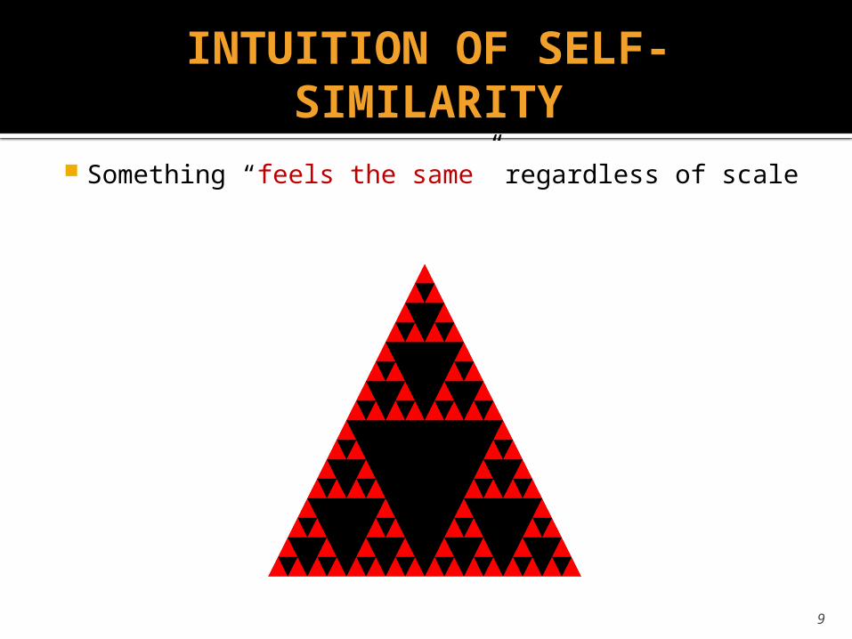
INTUITION OF SELF-SIMILARITY
Something “feels the same” regardless of scale
9
INTUITION OF SELF-SIMILARITY
10
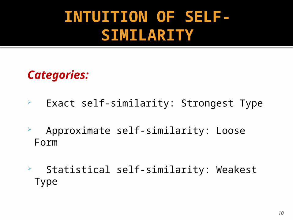
Categories:
Exact self-similarity: Strongest Type
Approximate self-similarity: Loose Form
Statistical self-similarity: Weakest Type

INTUITION OF SELF-SIMILARITY
11
Approximate self-similarity:
Recognisably similar but not exactly so.
e.g. Mandelbrot set
Statistical self-similarity:
Only numerical or statistical measures that are preserved
across scales
STOCHASTIC OBJECTS
In case of Stochastic Objects
e.g. time-series
Self-similarity is used in the distributional sense
12
WHY SELF-SIMILARITY IMPORTANT?
Recently, network packet traffic has been identified as being self-similar.
Current network traffic modeling using Poisson distributing (etc.) does not take into account the self-similar nature of traffic.
This leads to inaccurate modeling of network traffic. 13

PROBLEMS WITH CURRENT MODELS
A Poisson process When observed on a fine time scale will
appear bursty When aggregated on a coarse time scale
will flatten (smooth) to white noise
A Self-Similar (fractal) process When aggregated over wide range of
time scales will maintain its bursty characteristic
14
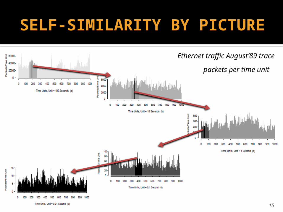
SELF-SIMILARITY BY PICTURE
15
packets per time unit
Ethernet traffic August’89 trace
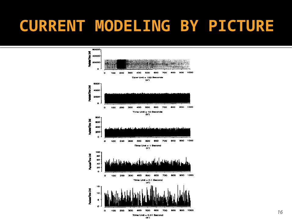
CURRENT MODELING BY PICTURE
16

SIDE-BY-SIDE VIEW
17
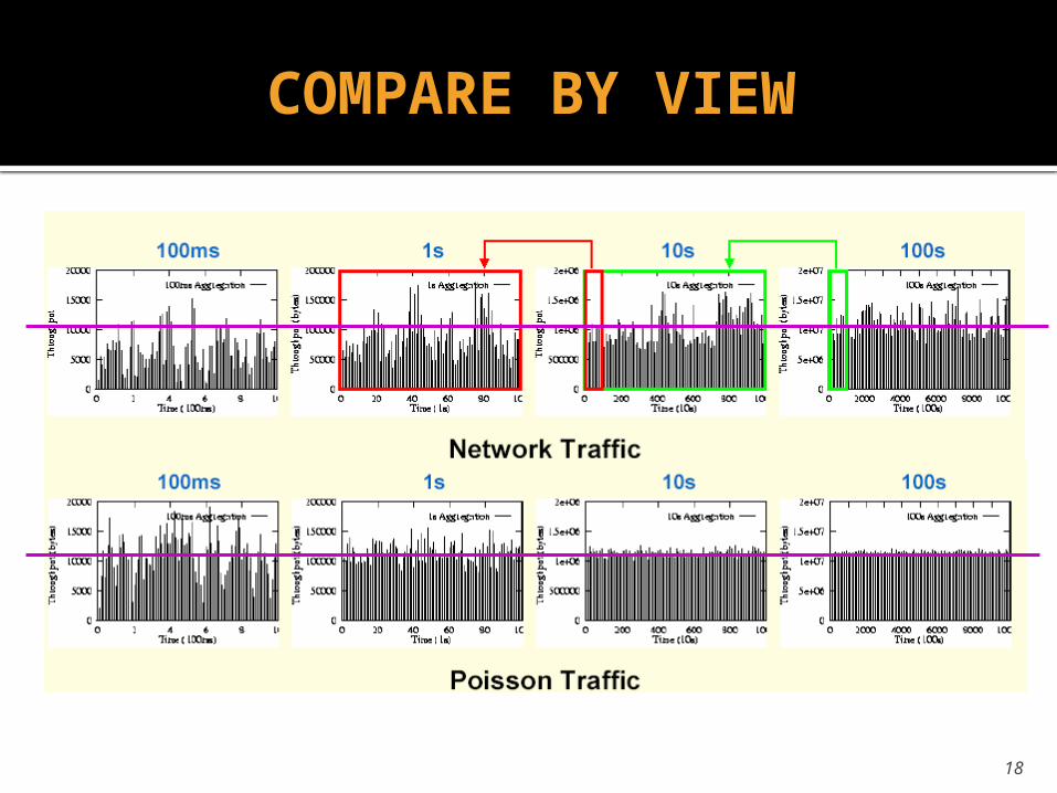
COMPARE BY VIEW
18

CONSEQUENCES OF SELF-SIMILARITY
19
Bursty Data
Streams
Aggregation
Smooth Pattern
Streams
Bursty Data
Streams
Aggregation
Bursty Aggregate
Streams
Reality (self-similar):
Current Model:
Consequence: Inaccuracy

MATHEMATICAL DEFINITIONS
Long-range Dependence autocorrelation decays slowly
Hurst Parameter Developed by Harold Hurst (1965) H is a measure of “burstiness”
▪ also considered a measure of self-similarity 0 < H < 1 H increases as traffic increases
▪ i.e., traffic becomes more self-similar20
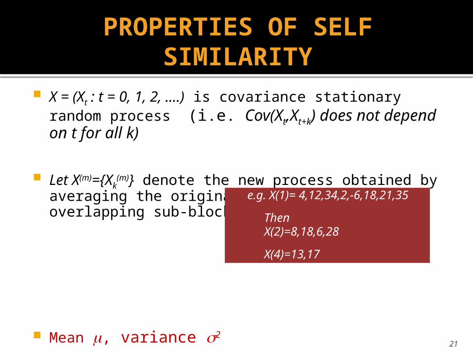
PROPERTIES OF SELF SIMILARITY
X = (Xt : t = 0, 1, 2, ….) is covariance stationary random process (i.e. Cov(Xt,Xt+k) does not depend on t for all k)
Let X(m)={Xk(m)} denote the new process obtained by
averaging the original series X in non-overlapping sub-blocks of size m.
Mean , variance 2
Suppose that Autocorrelation Function r(k) k -β, 0<β<1
21
e.g. X(1)= 4,12,34,2,-6,18,21,35
Then X(2)=8,18,6,28
X(4)=13,17

DEFINITION BY AUTO-CORRELATION
X is exactly second-order self-similar if The aggregated processes have the same
autocorrelation structure as X. i.e. r (m) (k) = r(k), k0 for all m =1,2, …
X is asymptotically second-order self-similar ifthe above holds when [ r (m) (k) r(k), m ]
Most striking feature of self-similarity: Correlation structures of the aggregated process do not degenerate as m 22
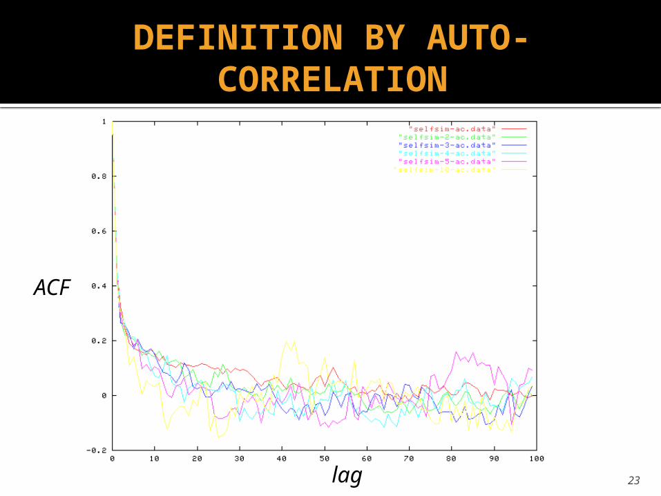
23lag
ACF
DEFINITION BY AUTO-CORRELATION

24
DEFINITION BY AUTO-CORRELATION
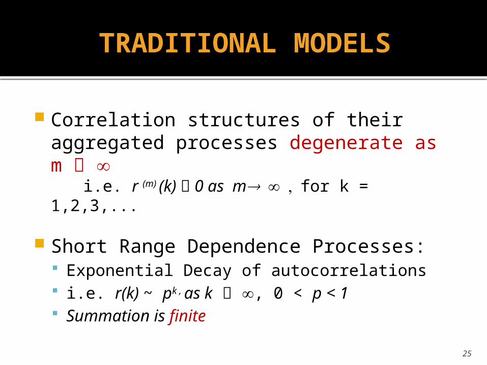
TRADITIONAL MODELS
Correlation structures of their aggregated processes degenerate as m i.e. r (m) (k) 0 as m , for k = 1,2,3,...
Short Range Dependence Processes: Exponential Decay of autocorrelations i.e. r(k) ~ pk , as k , 0 < p < 1 Summation is finite
25

LONG RANGE DEPENDENCE
Processes with Long Range Dependence are characterized by an autocorrelation function that decays hyperbolically as k increases
Important Property: This is also called non-summability of correlation
kkr )(
26
INTUITION
The intuition behind long-range dependence:
While high-lag correlations are all individually small, their cumulative affect is important
Gives rise to features drastically different from conventional short-range dependent processes
27

THE MEASURE OF SELF-SIMILARITY
Hurst Parameter H , 0.5 < H < 1
Three approaches to estimate H (Based on properties of self-similar processes) Variance Analysis of aggregated
processes Rescaled Range (R/S) Analysis for
different block sizes: time domain analysis
Periodogram Analysis: frequency domain analysis (Whittle Estimator)
28
!

VARIANCE ANALYSIS
Variance of aggregated processes decays as: Var(X(m)) = am-b as m infinite,
For short range dependent processes (e.g. Poisson Process):
Var(X(m)) = am-1 as m infinite,
Plot Var(X(m)) against m on a log-log plot
Slope > -1 indicative of self-similarity29

VARIANCE PLOT EXAMPLE
30
Slope=-1
Slope=-0.7

THE R/S STATISTIC
)],......,,0min(),......,,0[max()(
1
)(
)(2121 nn WWWWWW
nSnS
nR
)(),(
),,....2,1:(2 nSVarianceSamplenXmeanSample
nkX k
)()....( 21 nXkXXXW kk
31
where
For a given set of observations,
Rescaled Adjusted Range or R/S statistic is given by

EXAMPLE
Xk = 14,1,3,5,10,3
Mean = 36/6 = 6W1 =14-(1*6 )=8W2 =15-(2*6 )=3W3 =18-(3*6 )=0W4 =23-(4*6 )=-1W5 =33-(5*6 )=3W6 =36-(6*6 )=0 32
R/S = 1/S*[8-(-1)] = 9/S

THE HURST EFFECT
For self-similar data, rescaled range or R/S statistic grows according to cnH H = Hurst Paramater, > 0.5
For short-range processes , R/S statistic ~ dn0.5
History: The Nile river In the 1940-50’s, Harold Edwin Hurst studied the 800-year
record of flooding along the Nile river. (yearly minimum water level) Finds long-range dependence.
33

POX PLOT EXAMPLE
34
Slope = 1.0
Slope = 0.5
Slope = 0.79
WHITTLE ESTIMATOR
Provides a confidence interval
Property: Any long range dependent process approaches fractional Gaussian noise (FGN), when aggregated to a certain level
Test the aggregated observations to ensure that it has converged to the normal distribution 35
SUMMARY
Self-similarity manifests itself in several equivalent fashions:
Non-degenerate autocorrelations Slowly decaying variance Long range dependence Hurst effect
36

PART 2:
ETHERNET TRAFFIC IS SELF-SIMILAR

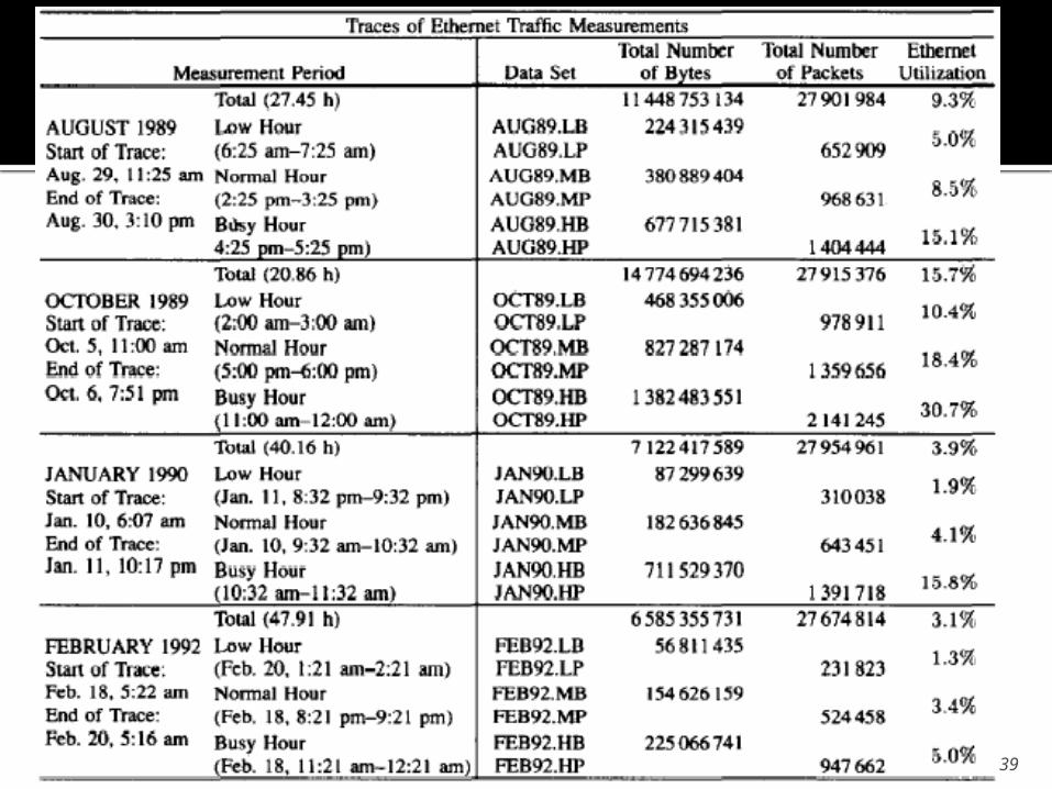
THE FAMOUS DATA
Leland and Wilson collected hundreds of millions of Ethernet packets without loss and with recorded time-stamps accurate to within 100µs.
Data collected from several Ethernet LAN’s at the Bellcore Morristown Research and Engineering Center at different times over the course of approximately 4 years.
38
39

PLOTS SHOWING SELF-SIMILARITY (Ⅰ)
40
H=0.5
H=0.5
H=1
Estimate H 0.8

PLOTS SHOWING SELF-SIMILARITY (Ⅱ)
41Higher Traffic, Higher H
High Traffic
Mid Traffic
Low Traffic
1.3%-10.4%
3.4%-18.4%
5.0%-30.7%
Packets
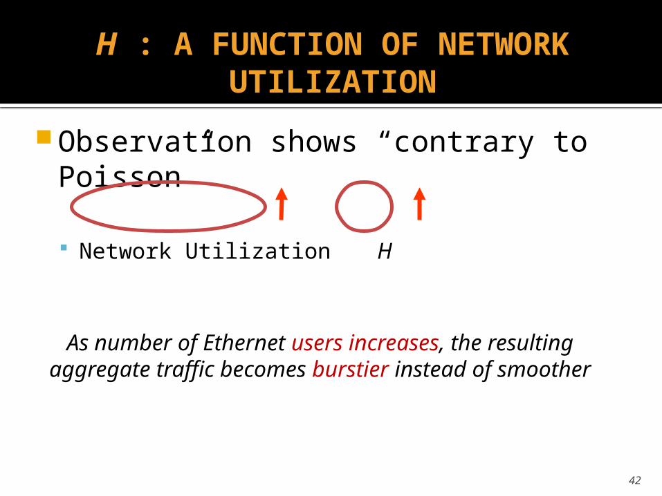
H : A FUNCTION OF NETWORK UTILIZATION
Observation shows “contrary to Poisson”
Network Utilization H
42
As number of Ethernet users increases, the resulting aggregate traffic becomes burstier instead of smoother

DIFFERENCE IN LOW TRAFFIC H VALUES
Pre-1990: host-to-host workgroup traffic
Post-1990: Router-to-router traffic
Low period router-to-router traffic consists mostly of machine-generated packets Tend to form a smoother arrival stream,
than low period host-to-host traffic43
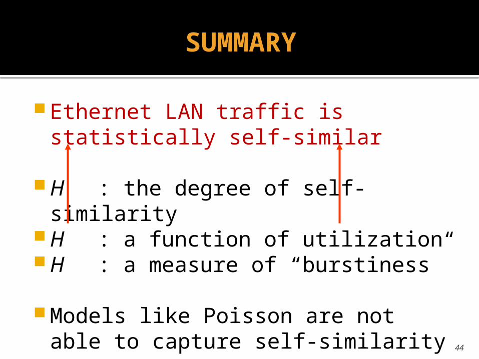
SUMMARY
Ethernet LAN traffic is statistically self-similar
H : the degree of self-similarityH : a function of utilizationH : a measure of “burstiness”
Models like Poisson are not able to capture self-similarity
44

PART 3:
IMPACT OF SELF SIMILARITY

COMPARISON
46

TWO EFFECTS
The superposition of many ON/OFF sources whose ON-periods and OFF-periods exhibit the Noah Effect produces aggregate network traffic that features the Joseph Effect.
47
Also known as packet train models
Noah Effect: high variability or infinite variance
Joseph Effect: Self-similar or
long-range dependent traffic
EXISTING MODELS
Traditional traffic models: finite variance ON/OFF source models
Superposition of such sourcesbehaves like white noise, with only short range correlations
48

EASY MODELING: NOAH EFFECT
Questions related to self-similarity can be reduced to practical implications of Noah Effect
Queuing and Network performance Network Congestion Controls Protocol Analysis
49
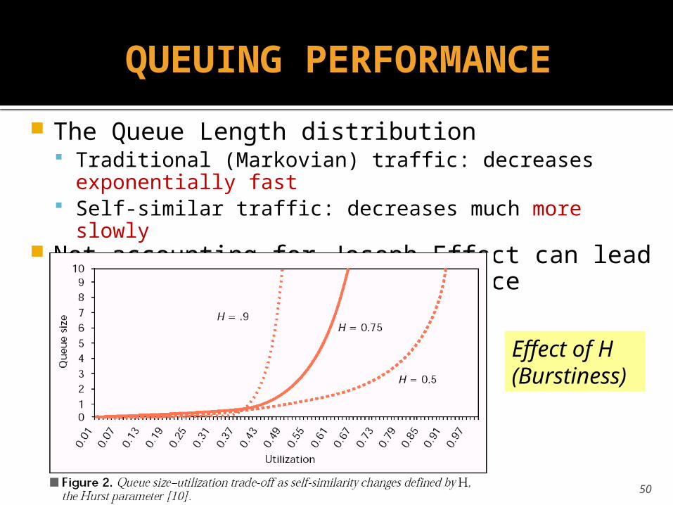
The Queue Length distribution Traditional (Markovian) traffic: decreases exponentially
fast Self-similar traffic: decreases much more slowly
Not accounting for Joseph Effect can lead to overly optimistic performance
50
Effect of H (Burstiness)
QUEUING PERFORMANCE
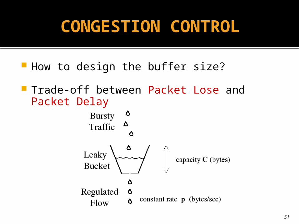
CONGESTION CONTROL
How to design the buffer size?
Trade-off between Packet Lose and Packet Delay
51
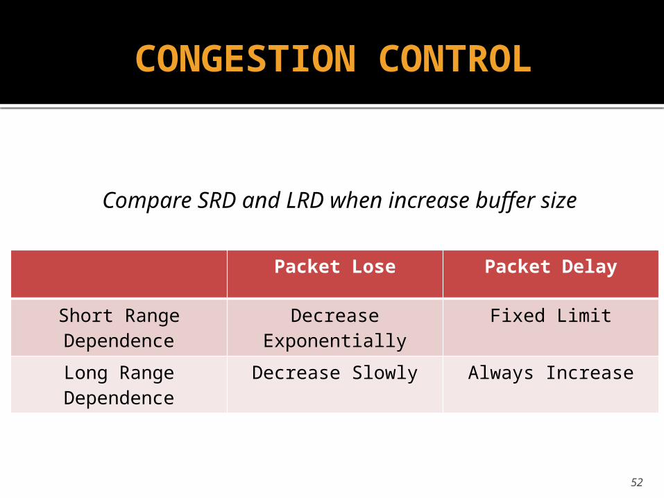
52
Packet Lose Packet Delay
Short Range Dependence
Decrease Exponentially
Fixed Limit
Long Range Dependence
Decrease Slowly Always Increase
Compare SRD and LRD when increase buffer size
CONGESTION CONTROL

PROTOCOL DESIGN
Protocol design should take into account knowledge about network traffic such as the presence or absence of the self-similarity.
53
Parsimonious Models Small number of parameters Every parameter has a physically meaningful
interpretation e.g. Mean , Variance 2, H Doesn’t quantify the effects of various factors in traffic
54
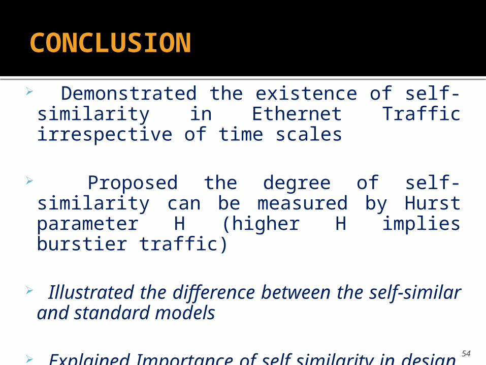
CONCLUSION
Demonstrated the existence of self-similarity in Ethernet Traffic irrespective of time scales
Proposed the degree of self-similarity can be measured by Hurst parameter H (higher H implies burstier traffic)
Illustrated the difference between the self-similar and standard models
Explained Importance of self similarity in design, control, performance analysis

A USEFUL LINK AND MATERIALS
55
http://ita.ee.lbl.gov/html/contrib/BC.html

Questions?
THANK YOU!