Embed Size (px)
Citation preview

2
LINEAR ALGEBRA
The algebraic properties of real numbers and matrices form the foundation for generalizations and abstractions that permit systematic analysis and solution of large scale engineering problems. Concepts of linear algebra are developed in this chapter, using familiar concepts of vector algebra and matrices. The goal here is to develop a mastery of the concepts and methods of linear algebra in a comfortable setting, prior to developing methods that encounter the technical complexities of differential equations and infinite dimensional spaces.
2.1 VECTOR ALGEBRA
In preparation for developing concepts and tools of linear algebra that form the foundation for more advanced methods presented in this text, it is helpful to review familiar concepts of vector algebra and to relate them to matrices. Geometric definitions of vector algebra are first recalled and related to operations with Cartesian components of vectors. It is then shown that all of these comfortable operations with vectors can be represented as matrix operations. The value of this form of vector algebra is two fold. First, it provides a geometric foundation for concepts of linear algebra that are essential in engineering analysis. Second, it reduces vector operations to a form that can be easily implemented on a digital computer.
Geometric Vectors
The concept of a vector may be introduced in a very general geometric setting, with no requirement for identification of a reference frame. In this setting a geometric vector, or simply a vector, is defined as the directed line segment from one point to another point in space. Its direction is therefore established and its magnitude is defined to be the distance between the points that are connected by the vector. This geometric setting for vector analysis, together with algebraic operations of addition, multiplication by a scalar, scalar product, and vector product form the classical foundation of vector analysis.
Vector 1 in Fig. 2.1.1, beginning at point A and ending at point B, is denoted by the notation ~, in its geometric sense. The magnitude of a vector 1 is its length (the distance between A and B) and is denoted by a, or 111. Note that the magnitude of a vector is positive if points A and B do not coincide and is zero only when they coincide. A vector
30

Sec. 2.1 Vector Algebra 31
with zero length is denoted 0 and is called the zero vector.
B
A
Figure 2.1.1 Vector from Point A to Point B
Definition 2.1.1. Multiplication of a vector 1 by a scalar a ~ 0 is defined as a vector in the same direction as 1, but having magnitude aa. A unit vector, having a length of a unity, in the direction 1 * 0 is ( 1/a ) 1. Multiplication of a vector 1 by a negative scalar ~ < 0 is defined as the vector with magnitude I ~ Ia and direction opposite to that of 1. The negative of a vector is obtained by multiplying the vector by -1. It is the vector with the same magnitude but opposite direction. •
Example 2.1.1
Let points A and B in Fig. 2.1.1 be located in an orthogonal reference frame, as shown in Fig. 2.1.2. The distance between points A and B, with coordinates (Ax, Ay, Az) and (Bx, By, Bz), respectively, is the magnitude of 1; i.e.,
z (B,B,B)
X y Z
(A ,A ,A) X y z
y
X
Figure 2.1.2 Vector Located in Orthogonal Reference Frame •
Definition 2.1.2. Addition of vectors 1 and it is according to the parallelogram rule, as shown in Fig. 2.1.3. The parallelogram used in this construction is formed in the plane that contains the intersecting vectors 1 and it. The vector sum is written as
~ ~ ~
a+ b = c (2.1.1)
32
[3]:
--+ u
--+ --+ 9(a,b)
Figure 2.1.3 Addition of Vectors
Chap. 2 Linear Algebra
• Addition of vectors and multiplication of vectors by scalars obey the following rules
--+ --+ --+ --+ a+b = b+a
--+ --+ --+ --+ a ( a+ b ) = a. a+ a.b
--+ --+ --+ (a.+P) a= a.a+Pa
(2.1.2)
where a and P are scalars. Orthogonal reference frames are used extensively in representing vectors. Use in this
text is limited to right-hand x-y-z orthogonal reference frames; i.e., frames with mutually orthogonal x, y, and z axes that are ordered by the finger structure of the right hand, as shown in Fig. 2.1.4. Such a frame is called a Cartesian reference frame. For indexing of variables, the x-y-z frame may be denoted by an x1-x2-x3 frame, as shown in Fig. 2.1.4.
Figure 2.1.4 Right-Hand Orthogonal Reference Frame
A vector 1 can be resolved into components a1, a2o and a3 along the xl> x2, and x3 axes of a Cartesian reference frame, as shown in Fig. 2.1.5. These components are called
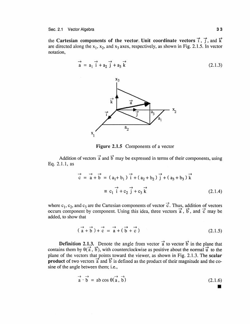
Sec. 2.1 Vector Algebra 33
the Cartesian components of the vector. Unit coordinate vectors 1, 1, and it are directed along the x1, x2, and x3 axes, respectively, as shown in Fig. 2.1.5. In vector notation,
~ ~ ~ ~
a = a1 i + a2 j + a3 k (2.1.3)
Figure 2.1.5 Components of a vector
Addition of vectors 1 and 'S may be expressed in terms of their components, using Eq. 2.1.1, as
~ ~ ~ ~ ~ ~
c = a+b = (a1+b1 ) i +(a2 +b2 ) j +(a3 +b3 )k
~ ~ ~
= c1 i + c2 j + c3 k (2.1.4)
where c1, c2, and c3 are the Cartesian components of vector C!. Thus, addition of vectors occurs component by component. Using this idea, three vectors 1, 'S, and (] may be added, to show that
~~~~~~
(a+b)+c = a+(b+c) (2.1.5)
Definition 2.1.3. Denote the angle from vector 1 to vector'S in the plane that contains them by ec1' 'S), with counterclockwise as positive about the normal ti to the plane of the vectors that points toward the viewer, as shown in Fig. 2.1.3. The scalar product of two vectors 1 and 'S is defined as the product of their magnitude and the cosine of the angle between them; i.e.,
~ ~ ~ ~
a · b = ab cos e( a , b ) (2.1.6)
•
34 Chap. 2 Linear Algebra
This definition is in purely geometric terms, so it is independent of the reference frame in which the vectors are represented. Note that if two vectors 1 and 'S are nonzero; i.e., a ::1:- 0 and b ::1:- 0, then their scalar product is zero if and only if cos 9(1, W) = 0. Two nonzero vectors are said to be orthogonal if their scalar product is zero. Since
rl-+ -+rl e a f . h 9(b, a)= 21t- 9( a, b) and cos (21t- ) =cos u, the order o terms appeanng on t e right side ofEq. 2.1.6 is immaterial. Thus,
(2.1.7)
Based on the definition of the scalar product, the following identities hold for the . di """"" """"" d~ umt coo11 nate vectors 1 , J , an A :
--+ --+ --+ --+ --+ --+ t·J=j·k=k·i=O
--+ --+ --+ --+ --+ --+ i·i=j·j=k·k=1
--+ Furthermore, for any vector a ,
--+ --+ 2 a · a = aa cos 0 = a
(2.1.8)
While not obvious on geometrical grounds, the scalar product satisfies the relation [2]
--+ --+ --+ --+ --+ --+ --+ (a+b)·c = a·c+b·c (2.1.9)
Using Eq. 2.1.9 and the identities ofEq. 2.1.8, a direct calculation yields
--+ --+ --+ --+ --+ --+ --+ --+ a · b = ( a1 i + a2 j + a3k )·( b1 i + b2 j + b3k )
(2.1.10)
Definition 2.1.4. The vector product of two vectors 1 and lJ is defmed as the vector
--+ --+ --+ --+ --+ a x b = ab sin 9( a , b) u (2.1.11)
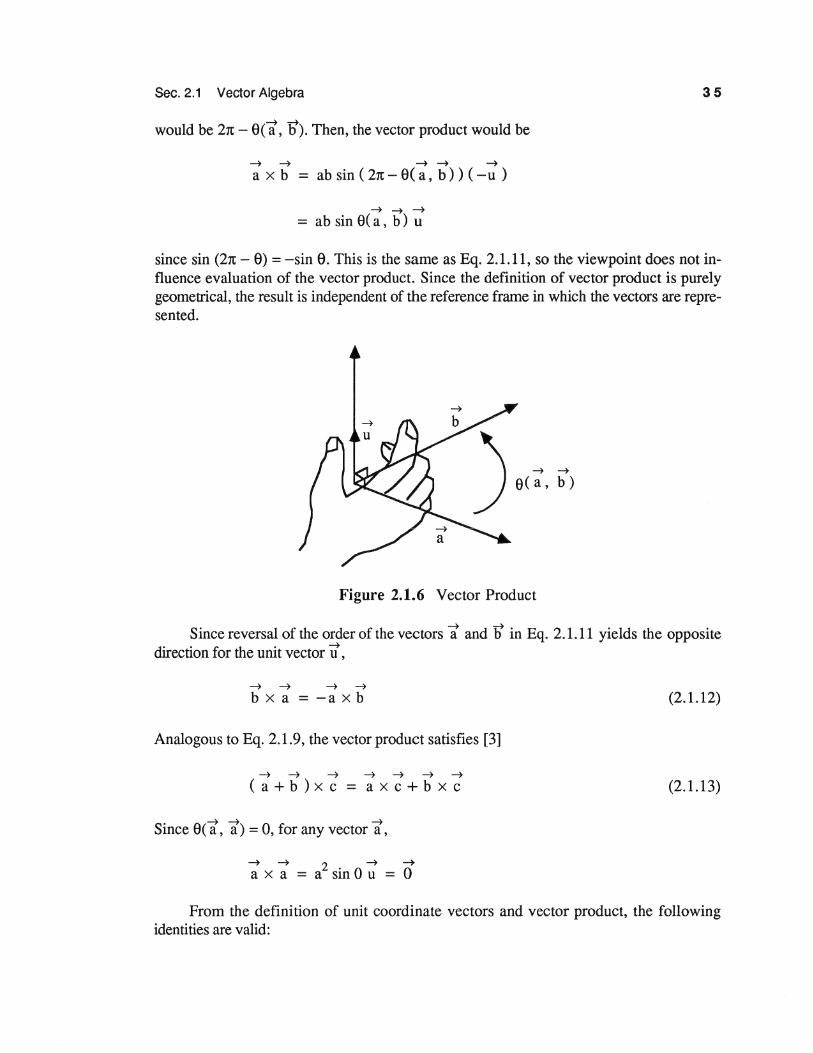
where ti is a unit vector that is orthogonal (perpendicular) to the plane that contains vectors 1 and 1), taken in the positive right-hand coordinate direction, as shown in Fig. 2.1.6. II
If the viewer were behind the plane of Fig. 2.1.6 that is formed by vectors 1 and lJ, the unit normal to the plane would be -ti and the counterclockwise angle from 1 to'S
Sec. 2.1 Vector Algebra 35
~ rl would be 27t - e( a, b). Then, the vector product would be
~ ~ ~ ~ ~
a X b = ab sin ( 21t- e( a, b)) ( -U )
~ ~--+
= ab sin e( a ' b) u
since sin (27t- e) =-sin e. This is the same as Eq. 2.1.11, so the viewpoint does not influence evaluation of the vector product. Since the definition of vector product is purely geometrical, the result is independent of the reference frame in which the vectors are represented.
Figure 2.1.6 Vector Product
Since reversal of the order of the vectors 1 and 1t in Eq. 2.1.11 yields the opposite direction for the unit vector 11,
~ ~ ~ ~
b x a = -ax b
Analogous to Eq. 2.1.9, the vector product satisfies [3]
~~ ~ ~~~~
(a+b)xc = axc+bxc
Since e(1, 1) = 0, for any vector 1,
~ ~ 2 ~ --+ axa=asinOu=O
(2.1.12)
(2.1.13)
From the definition of unit coordinate vectors and vector product, the following identities are valid:
3 6 Chap. 2 Linear Algebra
--+ --+ --+ --+ --+ -+ --+ ixi=jxj=kxk=O
--+ --+ --+ --+ --+ ixj=-jxi=k
--+ --+ --+ --+ --+ (2.1.14)
jxk =-kxj = i
--+ --+ --+ --+ --+ kxi=-ixk=j
Using the identities of Eqs. 2.1.14 and the property of vector product of Eq. 2.1.13, the vector product of two vectors may be expanded and written in terms of their components as
--+ --+ --+ --+ --+ --+ c = a x b = ( a2b3 - a3b2 ) i + ( a3b1 - a1 b3 ) j + ( a1 b2 - a2b1 ) k
--+ --+ --+ = c1 i + c2 j + c3 k (2.1.15)
Algebraic Vectors
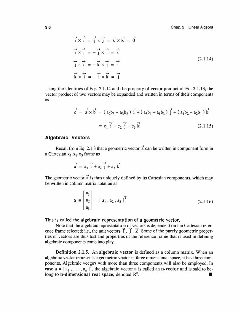
Recall from Eq. 2.1.3 that a geometric vector 1 can be written in component form in a Cartesian x1-xTx3 frame as
--+ --+ --+ --+ a = a1 i + a2 j + a3 k
The geometric vector 1 is thus uniquely defined by its Cartesian components, which may be written in column matrix notation as
(2.1.16)
This is called the algebraic representation of a geometric vector. Note that the algebraic representation of vectors is dependent on the Cartesian refer
ence frame selected; i.e., the unit vectors T, J, it. Some of the purely geometric properties of vectors are thus lost and properties of the reference frame that is used in defining algebraic components come into play.
Definition 2.1.5. An algebraic vector is defined as a column matrix. When an algebraic vector represents a geometric vector in three dimensional space, it has three components. Algebraic vectors with more than three components will also be employed. In case a= [ a1 , ... , Rn ]T, the algebraic vector a is called ann-vector and is said to belongton-dimensional real space, denoted Rn. •

Sec. 2.1 Vector Algebra
If two geometric vectors 1 and 'S are represented in algebraic form as
T a = [ a1, a2, a3 ]
37
(2.1.17)
(2.1.18)
then their vector sum t = 1 + 'S, fromEq. 2.1.4, is represented in algebraic form by
c=a+b
Example 2.1.2
The algebraic representation of geometric vectors
is
~ ~ ~ ~
a = i + 2j + 3k
~ ~ ~ ~
b=-i+j-k
T a= [ 1, 2, 3]
T b=[-1,1,-1]
The algebraic representation of the sum t = 1 + 'S is
c =a + b = [ 0 , 3 , 2 ]T
(2.1.19)
• Two geometric vectors are equal; i.e., 1 = 'S, if and only if the Cartesian compo
nents of the vectors are equal; i.e., a = b. Multiplication of a vector 1 by a scalar a occurs component by component, so the geometric vector a 1 is represented by the algebraic vector aa.
Since there is a one-to-one correspondence between geometric vectors and 3x1 algebraic vectors that are formed from their Cartesian components in a specified Cartesian reference frame, no distinction other than notation will be made between them in the remainder of this text
The scalar product of vectors 1 and "S may be expressed in algebraic form, using the result of Eq. 2.1.10, as
(2.1.20)
Example 2.1.3
The scalar product of vectors 1 and "S (or a and b) in Example 2.1.2 is

38 Chap. 2 Linear Algebra
[-1] ~ ~ T a · b = a b = [ 1 , 2, 3] !
1 = -2
From the defmition of scalar product,
a Tb = ab cos S(a, b)
and, with a= (aTa)112 = ...JT4 and b = (bTbi12 = ...J3, cos S(a, b)= -2N42. Thus, S(a, b) = 1.88 or 4.40 rad. •
A skew symmetric matrix a, associated with a 3x1 algebraic vector a, is defined as
(2.1.21)
Note that an overhead- (pronounced tilde) indicates that the components of vector a are used to generate a skew symmetric 3x3 matrix a.
The vector product t = 1 x W, which is expanded in component form in Eq. 2.1.15, can be written in algebraic vector form as
(2.1.22)
A direct computation verifies that
- -ab = -ba
which agrees with the vector product property of Eq. 2.1.12.
Example 2.1.4
The algebraic representation of the vector product t = 1 x W in Example 2.1.2 is
• For later use, it is helpful to recall a fundamental property of the - operation; i.e.,
Sec. 2.2 Vector Spaces 39
-T [ -~, a3 -•z] a 0 al =-a (2.1.23) a2 -al 0
The reduction of geometric concepts of vector algebra to matrix algebra in this section provides insights and computational tools that are needed later in the text and in applications. The reader is encouraged to return to this intuitively clear relationship between three dimensional geometry and matrix algebra when concepts of higher dimensional analysis become more complex.
EXERCISES 2.1
1. Verify Eq. 2.1.5.
2. Verify Eq. 2.1.9.
3. Verify Eq. 2.1.15.
4. For;iven vectors 1 = f + 2] + 3lt and W = 4] + 5lt, find 1 + W, 1· W, and 1 x b . Also find a + b, aT b, and ab, using algebraic representations a and b of 1 and W, respectively.
5. Repeat Exercise 4 for the vectors 1 = 5f + 2 J + it and W = 2f + 6] + 4lt.
2.2 VECTOR SPACES
Matrix analysis, which is reviewed in Chapter 1, is of importance in its own right and serves as a model for more general methods of engineering analysis. For this reason, it is important to obtain proficiency in viewing linear calculations and matrix analysis in avector space setting. Vector space concepts and techniques that generalize methods presented in Section 2.1 provide a rational setting that allows a clear view of the forest, without getting bogged down in all the notational trees that arise in complex problems. The contents of this section should be viewed by the reader as both tools for use in computational algebra and a conceptual base for methods of engineering analysis that follow.
n-Dimensional Real Space (R")
It is conventional to speak of an nxl matrix as a column vector, or simply as a vector. The collection of all such vectors is called n-dimensional real space and is denoted Rn. A vector in Rn is thus
A row matrix [ x1, x2, ... , Xn ], which is the transpose of the column matrix x, is called a row vector and is denoted by x T.
40 Chap. 2 Linear Algebra
Vectors in Rn follow the same laws of addition and multiplication by a scalar as three dimensional vectors in Section 2.1. These laws are typical of an algebraic system called a vector space.
Definition 2.2.1. A vector space V is a set of vectors with operations of addition and multiplication by a real scalar that satisfy the following vector space postulates:
(1) Closure under addition; For every pair of vectors x andy in V there is a unique sum denoted by x + y in V.
For vectors x, y, and z in V, (2) ( X + y ) + Z = X + ( y + Z )
(3) X+ y = y +X (4) A zero vector 0 exists, such that x + 0 = x, for all x (5) A negative vector -x exists for all x, such that x + ( -x ) = 0 (6) Closure under multiplication by a scalar; For every real scalar a and
every vector x in V there is a unique vector ax in V. For real scalars a and ~ and vectors x and y in V,
(7) a ( x + y ) = ax + a.y (8) ( a + ~ ) x = ax + ~x (9) ( a.~ ) X = a ( ~X ) (10) lx=x •
Note that there need not be any concept of magnitude of vectors or products of vectors as part of the definition of a vector space. These and additional operations and properties may be associated with the underlying vector space, to enrich its structure and make it more useful for specific engineering applications. It is important to realize, however, that many of these add-on properties make sense only if the basic vector space algebraic properties are well defined.
In order to specify a vector space, and since many different vector spaces are used in engineering analysis, a set V of vectors with operations of addition and multiplication by a real scalar that satisfy all the properties of Definition 2.2.1 must be defined. For example, the set R 1 of real numbers is a vector space, where addition and multiplication by a scalar are the usual addition and multiplication of real numbers. In this case, a real number plays the role of both a vector and a scalar.
Example 2.2.1
Consider the set* of vectors
* Set notation used in this text is limited to defining subsets of the form
{ x E S: condition satisfied by x }
where S is a given set and the condition following the colon must be satisfied by each x in the subset.
Sec. 2.2 Vector Spaces 41
with addition and multiplication by a scalar defined by matrix operations of Section 1.2. Properties (2) - (5) and (7) - (10) of Definition 2.2.1 hold, since they are properties of addition and multiplication by scalars in Rn. Property 2.2.1 holds, since if x e E andy e E, then x1 = y1 = 0. Thus for z = x + y, z1 = x1 + y1 = 0, so z e E and E is closed under addition. Likewise, if x e E, then for z = ax where a is any scalar, z1 = ax1 = 0, so z e E and E is closed under multiplication by a scalar.
To make this example more concrete, let n = 3. Then E = { x e R3: x1 = 0} is a collection of vectors that lie in the x2-x3 plane. •
Example 2.2.1 illustrates that when a candidate vector space is defmed as a subset of a known vector space, then properties (2) - (5) and (7) - ( 10) of Definition 2.2.1 automatically follow. Therefore, in this case, only properties (1) and (6) need to be verified.
Example 2.2.2
As a second example, let
F = { x e Rn: x1 = 1 }
For x e F andy e F, x1 = y1 = 1. Defining z = x + y, z1 = x1 + y1 = 2. Hence, z e F, so F is not closed under the operation of addition. Thus it is not a vector space. •
Linear Independence of Vectors
Definition 2.2.2. A set of vectors xl, x2, ... , xn is said to be linearly dependent if there exist scalars c1, c2, ... , Cn that are not all zero, such that
c·xi = 0 1 (2.2.1)
where summation notation is used. If a set of vectors is not linearly dependent, then it is said to be linearly independent. Equivalently, a set of vectors xl, x2, ... , xn is linearly independent if cixi = 0 implies that ci = 0, for all i. •
The last observation of Definition 2.2.2 forms a convenient means of testing for linearly independence. Simply write down Eq. 2.2.1 and treat it as a set of equations in the variables ci, with the known vectors xi as coefficients. If the only solution is c1 = ... = cn = 0, then the xl, x2, ... , xn are linearly independent.
If any vector xk among a set xl, x2, ... , xn is zero, then the set is linearly dependent. To see that this is true, let xk = 0, choose Cj = oik, and note that cixi = oikxi = xk = 0. Since ck = 1, not all the ci are zero and the xi are linearly dependent.
Example 2.2.3
Consider the vector space R3 and vectors xl = [ 1, 0, 0 ]T, x2 = [ 1, 1, 0 ]T, and x3 = [ 1, 1, 1 ]T. To determine whether xl, x2, and x3 are linearly independent,

42 Chap. 2 Linear Algebra
form the equation
Since the determinant of the coefficient matrix is 1, it is nonsingular and c1 = c2 = c3 = 0 is the only solution. Thus, the vectors are linearly independent. •
Example 2.2.4
Consider again the vector space R3 and vectors
To check for linear independence, form
[ 1 3 0 2] Ct [0] ci xi = 2 6 1 5 cz = 0
-1 0 0 0 c3 0 c4
A solution may be obtained for c1, c3, and c4 as functions of c2,
Ct =0 c4 = -3c2 /2 c3 =- ( 6c2 + 5c4 ) = 3c2 /2
which is valid for any nonzero value of c2; e.g., c2 = 1. Thus the xi are not linearly independent; i.e., they are linearly dependent. •
Definition 2.2.3. A set of vectors xl, x2, ... , xn in a vector space Vis said to span the vector space if every vector in the space can be written as a linear combination of the set; i.e., for every vector x in V, there exist scalars c1, c2, ... , cn, such that
X= C·Xi 1
Example 2.2.5
(2.2.2) •
Consider the vectors xl = [ 1, 2, 1 ]T, x2 = [ 1, 0, 2 ]T, and x3 = [ 1, 0, 0 ]Tin R3. To find out whether { xl, x2, x3 } spans R3, choose any vector a= [ a1, az, a3 ]Tin
Sec. 2.2 Vector Spaces 43
=a
Direct manipulation yields the solution
Thus, { x1, x2, x3 } spans R3. • A set of vectors x1, x2, ... , xn may span a vector space and still not be linearly in
dependent. However, if the vectors are linearly dependent, a subset can be selected that is linearly independent and also spans the same space. To see that this is true, suppose x 1, x2, ... , xn span the space and are linearly dependent. Then there exists a set of scalars 'Y1• y2, ... , 'Yn that are not all zero, such that
Without loss of generality, assume that 'Yn :-1: 0. Then, xn can be written in terms of x 1, x2, ... 'xn-1 as
'Y1 1 'Y2 2 'Yn-1 n-1 -x- -x - ... --x 'Yn 'Yn 'Yn
For any vector x in the vector space, there exist ci, i = 1, ... , n, such that
X= C·Xi 1
[ 'Y1 1 'Y2 2 'Yn-1 n-1 ] +en --x- -x - ... ---x 'Yn 'Yn 'Yn
Therefore, the subset x 1, x2, ... , xn-1 spans the space. If this subset is linearly dependent, the process can be repeated. Eventually, a subset x1, x2, ... , xm, with m < n, will be obtained that spans the space and is linearly independent.
Basis and Dimension of Vector Spaces
Definition 2.2.4. A basis of a vector space is a set of linearly independent vectors that spans the space. •
44 Chap. 2 Linear Algebra
Example 2.2.6
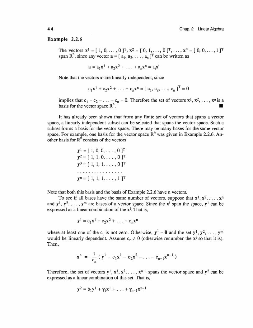
The vectors xl = [ 1, 0, ... , 0 ]T, x2 = [ 0, 1, ... , 0 ]T, ... , xn = [ 0, 0, ... , 1 ]T span Rn, since any vector a = [ a1, a2, ... , ~ ]T can be written as
Note that the vectors xi are linearly independent, since
implies that c1 = c2 = ... = cn = 0. Therefore the set of vectors x 1, x2, ... , xn is a basis for the vector space Rn. •
It has already been shown that from any finite set of vectors that spans a vector space, a linearly independent subset can be selected that spans the vector space. Such a subset forms a basis for the vector space. There may be many bases for the same vector space. For example, one basis for the vector space Rn was given in Example 2.2.6. Another basis for Rn consists of the vectors
yl = [ 1, 0, 0, ... , 0 ]T y2 = [ 1, 1, 0, ... , 0 ]T
y3 = [ 1, 1, 1, ... , 0 ]T
yn = [ 1, 1, 1, ... , 1 ]T
Note that both this basis and the basis of Example 2.2.6 haven vectors. To see if all bases have the same number of vectors, suppose that xl, x2, ... , xn
and yl, y2, ... , ym are bases of a vector space. Since the xi span the space, yl can be expressed as a linear combination of the xi. That is,
where at least one of the ci is not zero. Otherwise, y1 = 0 and the set yl, y2, ... , ym would be linearly dependent. Assume cn :t 0 (otherwise renumber the xi so that it is). Then,
Therefore, the set of vectors yl, xl, x2, ... , xn-t spans the vector space and y2 can be expressed as a linear combination of this set. That is,

Sec. 2.2 Vector Spaces 45
where at least one of the 'Yi is not zero. Otherwise yl and y2 would be linearly dependent. Thus, one of the xi, whose coefficient is not zero, can be written in terms of yl, y2, and the n-2 other xi. These vectors thus span the space. After repeating this process m times, a set of vectors yl, y2, ... , ym, with n- m;;::: 0, of the xi remain that span the space. Otherwise, the yi are linearly dependent. This argument can be applied with the roles of the xi and yi interchanged, leading to the conclusion that m - n ;;::: 0. The result n = m follows. Thus, all bases of the same vector space have the same number of vectors. This result justifies the following definition.
Definition 2.2.5. The dimension of a vector space is the minimun number of nonzero vectors that span the space. A vector space is called a finite dimensional vector space if it can be spanned by a finite number of vectors. •
To find the dimension of a finite-dimensional vector space, it is sufficient to demonstrate that a set of vectors is a basis and to count the number of vectors in the set. Thus, Example 2.2.6 verifies that the space Rn of nx1 column vectors is an n-dimensional vector space.
Theorem 2.2.1. The number of vectors in every basis of a finite dimensional vector space is the same and is equal to the dimension of the space. Further, every vector in the space can be represented by a unique linear combination of vectors in a basis. •
To prove the last part of Theorem 2.2.1, suppose that some vector x has two repre-.. fhb' 12 n' sentauons m terms o t e as1s x , x , ... , x ; I.e.,
Then,
0 = X - X = ( ~ - bi) xi
Since the xi are linearly independent, ai - bi = 0, for all i, and the representation is indeed unique. •
Suppose that ann-dimensional vector space V has a basis xl, x2, ... , xn. Relative to this basis, every vector in the space has a unique representation in terms of n scalars. There is, therefore, a one-to-one correspondence between the vector space V and the vector space Rn of nx 1 column vectors. Furthermore, if x = aixi and y = bixi, then x + y = ( ~ + bi) xi. If a is a scalar, ax = ( aai) xi. Therefore, addition of vectors and multiplication of vectors by a scalar is equivalent to carrying out these operations on column matrices (i.e., vectors in Rn) of the coefficients that represent the vectors in terms of a basis. This conclusion pf;rmits limiting the study of finite dimensional vector spaces to a study of the space Rn. Note that this is just a generalization of the conclusion drawn in Section 2.1 that geometric vectors in three dimensional space can be represented by column vectors in R3•

46 Chap. 2 Linear Algebra
Subs paces
Definition 2.2.6. Let V be a vector space and let S be a subset of V; i.e., if x e S, then x e V. If Sis a vector space with respect to the same operations as those in V, then S is called a subspace of V. •
Example 2.2. 7
An example of a subspace S of a vector space V is the space of all possible linear combinations of a subset { xl, ... , xn} of vectors from V; i.e.,
S = { x e V: x = c.xi, c. e R } 1 1
If the subset { xl, ... , xn} is linearly independent and is not a basis of V, then the subspace S is a proper subspace of V; i.e., it is not the whole space. A specific example of a proper subspace is the subspace S of R 3 that is spanned by the vectors [ 1, -1,0 ]T and [ 0, 1,-1 ]T; i.e.,
This two-dimensional subspace consists of the plane that contains the two given vectors and the origin. •
Theorem 2.2.2. Let V be a vector space and letS be a non-empty subset of V, with addition and multiplication by a scalar defined as in V. Then, S is a subspace of V if and only if the following conditions hold:
(1) If x andy are any vectors in S, then x + y is in S. (2) If a is any real number and x is any vector in S, then ax is in S. • The proof of Theorem 2.2.2 follows from Definition 2.2.1 of vector space and the
observation already made in Example 2.2.1.
Example 2.2.8
Consider the system of homogeneous linear equations Ax = 0, where A is an mxn matrix and x e Rn. A solution consists of a vector x = [ x1, x2, ... , xn ]T; i.e., a vector in Rn. Thus the set of all solutions is a subset of Rn. It may be shown that this is a subspace of Rn by verifying conditions (1) and (2) of Theorem 2.2.2.
Let xl and x2 be solutions of Ax= 0. Then xl + x2 is a solution, because A( xl + x2) = Axl + Ax2 = 0 + 0 = 0. Also, if x is a solution, then ax is a solution, because A( ax)= a( Ax)= aO = 0.
It should be noted that the set of all solutions to the system of nonhomoge-neous linear equations Ax= c, c ~ 0, is not a subspace of Rn. •

Sec. 2.2 Vector Spaces 47
EXERCISES 2.2
1. Determine the dimension of the vector space spanned by each of the following sets of vectors:
(a) [ 1, 1, 0 ]T, [ 1, 0, 0 ]T, [ 0, 1, 1 ]T (b) [ 1, 0, 0 ]T, [ 0, 1, 0 ]T, [ 0, 0, 1 ]T, [ 1, 1, 1 ]T (c) [ 1, 1, 1 ]T, [ 1, 0, 0 ]T, [ 1, 2, 1 ]T
2. Determine whether the vector [ 6, 1, -6, 2 ]T is in the vector space spanned by the vectors [ 1, 1, -1, 1 ]T, [ -1, 0, 1, 1 ]T, and [ 1, -1, -1,0 ]T.
3. LetS be the subspace ofR3 spanned by [ 1, 2, 2 ]T, [ 3, 2, 1 ]T, [ 11, 10,7 ]T, and [ 7, 6, 4 ]T. Find a basis for S. What is the dimension of S?
4. Which of the following subsets of R3 are subspaces?
(a) S consists of all vectors of the form [ a, b, 1 ]T and a and b are real. (b) S consists of all vectors of the form [ a, b, 0 ]T and a and b are real. (c) S consists of all vectors of the form [a, b, c ]T and a, b, and care real, where
a+ b =c. (d) S consists of all vectors of the form [a, b, c ]T and a, b, and care real, where
a=b.
5. Show that the collection of all polynomials of degree three or less; i.e., P = { a + bx + cx2 + dx3: a, b, c, and d are real and -oo < x < oo } is a four-dimensional vector space.
6. Are the vectors [ 0, -1, 0 ]T, [ 0, 1, -1]T, and [ 1, -2, 1 ]T linearly dependent? Can [ -2, 1, -3 ]T be expressed as a linear combination of these vectors? Express your result both geometrically and in terms of solutions of linear algebraic equations.
7. Prove that in an n-dimensional vector space, any set of n + 1 vectors is linearly dependent.
8. Prove Theorem 2.2.2.
9. What is the dimension of the subspace of R4 spanned by the vectors

48 Chap. 2 Linear Algebra
10. Which of the following subsets ofRn is a vector space?
(a) { X E Rn: X + [ 1, 0, ... , 0 ]T = 0 } (b) { X e Rn: xT[ 1, 0, ... , 0 ]T = 0 } (c) { x e Rn: x = a.y + ~z, y and z e Rn and a and ~ are arbitrary real scalars }
11. Which of the following subsets of R3 is a subspace?
(a) { X e R3: x1 = 1 } (b) { x e R3: x =a[ 1, 1, 0 ]T + ~[ 2, 2, 0 ]T , a and ~ are real } (c) { x e R3: x1x2 = 0 } (d) { x e R3: x1 + 2x2 - 3x3 = 0 }
If it is a subspace, what is its dimension?
12. Given a basis { [ 1, 0, 0 ]T, [ 0, 2, 2 ]T, [ 0, -1, 1 ]T } of R3, represent a vector [a, b, c ]T e R3 by a linear combination of vectors in the basis. Is the representation unique?
13. Which of the following subsets of Rn are subspaces of Rn?
(a) { x e Rn: x T y = 0, for a given y e Rn } (b) { X E Rn: X T X ~ 1 }
14. Show that the collection F of all real functions defined on the interval 0 ~ x ~ 1 is a vector space, where addition and multiplication by a scalar are defined by
(f+g)(x)=f(x)+g(x) (a.f)(x)=a.f(x)
where f and g are in F and a is a real number.
2.3 RANK OF MATRICES AND SOLUTION OF MATRIX EQUATIONS
The matrix theory outlined in Section 1.2 and the theory of finite dimensional vector spaces of Section 2.2 may now be exploited to develop both the basic theory and techniques for solution of matrix equations.
A common problem in engineering analysis is to find a set of n real variables x1, x2,
••• , Xn that represent physical quantities of displacement, velocity, stress, pressure, temperature, etc., and satisfy a set of m linear equations
no sum on n (2.3.1)

Sec. 2.3 Rank of Matrices and Solution of Matrix Equations 49
where the parameters au, a21, ... , ~and c1, c2, .•• , cm are given real constants. To solve a linear equation requires the following:
(1) determine whether a solution exists (2) find a solution, if one exists (3) determine whether the solution found is unique
The most conclusive method of demonstrating that a solution exists is to construct a solution; i.e., success in step (2) implies success in step (1). However, if no solution exists, all attempts to fmd a solution, no matter how time consuming or costly, will fail. It is thus prudent to first consider the question of existence of a solution. Finally, if there are multiple solutions, the engineer should be aware of this possibility (step 3) and may want to know all possible solutions.
In order to simplify Eq. 2.3.1, matrix notation is used; i.e.,
Ax =c (2.3.2)
where A = [ 3jj ] is the given mxn coefficient matrix, c = [ ci ] is a given mx 1 column matrix, and x = [ xi ] is the nx 1 column matrix of variables.
Rank of a Matrix
Definition 2.3.1. Let A = [ aij] be an mxn matrix. The rows of a matrix A are denoted a~ = [au, a12, •.. , a1n ], ... , ~ = [ Sml• Sm2, ..• , Smn ]. Considered as row vectors in Rn, they span a subspace of Rn that is called the row space of a matrix A. Similarly, the columns of a matrix A, a~ = [ a11 , a21 , .•. , Sml ]T, ••. ,
~ = [ a1n, ~n• ... , Smn ]T, span the column space of A, which is a subspace of Rm .
• Example 2.3.1
Consider again the vectors of Example 2.2.5,
1 [ ]T 2 T 3 T X = 1,2,1 , X = [1,0,2], X = [1,0,0]
If they are columns of matrix A, then
[ 1 1 1]
A= 2 0 0 1 2 0
Since it was shown in Example 2.2.5 that these vectors span the space R3, the column space of A is R3. •
Definition 2.3.2. The dimension of the row space of A is called the row rank of A; i.e., the number of linearly independent rows of A. Similarly, the column rank of A is the dimension of the column space of A; i.e., the number of linearly independent columns of A. •
50 Chap. 2 Linear Algebra
Example 2.3.2
In Example 2.3.1, the dimension of the column space of A is 3, since A has 3 linearly independent columns. Thus the column rank of A is 3. A simple calculation shows that the rows of A are also linearly independent. Thus, the row rank of A is also 3. •
Elementary Row Operations
Definition 2.3.3. An elementary row operation is one of the following operations on a matrix:
(1) the interchange of a pair of rows (2) the multiplication of a row by a nonzero scalar (3) the addition of one row to another row
These elementary row operations can be performed on an mxn matrix by multiplying on the left by elementary matrices that are obtained by performing the same operations on mxm identity matrices. •
The reader may recall that the concept of elementary matrices was introduced for 3x3 matrices in Section 1.3.
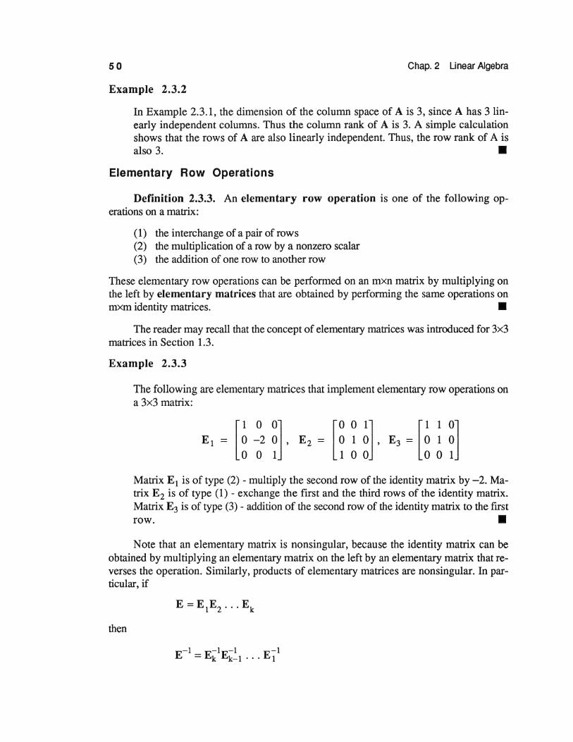
Example 2.3.3
The following are elementary matrices that implement elementary row operations on a 3x3 matrix:
[ 1 0 OJ [ 0 0 lJ [ 1 1 OJ E 1 = 0 -2 0 , E2 = 0 1 0 , E3 = 0 1 0 001 100 001
Matrix E 1 is of type (2) - multiply the second row of the identity matrix by -2. Matrix E 2 is of type (1)- exchange the first and the third rows of the identity matrix. Matrix E3 is of type (3) - addition of the second row of the identity matrix to the first
row. •
Note that an elementary matrix is nonsingular, because the identity matrix can be obtained by multiplying an elementary matrix on the left by an elementary matrix that reverses the operation. Similarly, products of elementary matrices are nonsingular. In particular, if
then
E-1 _ E-1E-1 E-1 - k k-1 . . . 1

Sec. 2.3 Rank of Matrices and Solution of Matrix Equations 51
Theorem 2.3.1. If B = EA, where E is a product of elementary matrices, then the row rank of A and the row rank of B are equal. •
To prove Theorem 2.3.1, suppose B = EA. Then the rows of B are obtained from the rows of A by the three elementary row operations. Thus, each row of B is a linear combination of the rows of A. Hence, the row space of B is contained in the row space of A. On the other hand, since A= E-lB, the row space of A is contained in the row space of B. Hence, the row spaces of A and B are identical and the row rank of A and row rank of B are equal. •
Example 2.3.4
To find the row rank of the matrix
A = [~ ~ ~] 3 4 2
note that
[ 1 3 2] EA = B = 2 1 0
0 0 0
where E is the product of elementary matrices that (1) multiply the third row by -1, (2) add the first row to the third row, and (3) add the second row to the third row; i.e.,
E = [~ ~ ~] [~ ~ ~] [~ ~ ~] = [~ ~ ~] 0 1 1 1 0 1 0 0 -1 1 1 -1
Hence the row rank of A is two. • Theorem 2.3.2. The row rank and the column rank of an mxn matrix A are
equal. •
For a proof of Theorem 2.3.2, the reader is referred to Ref. 1 (p. 74). Since the row and column rank of a matrix are equal, they will be referred to simply
as the rank of the matrix.
Example 2.3.5
Consider the matrix

52 Chap. 2 Linear Algebra
Combinations of elementary operations yield
[ 1-1J[4 3 1J [3 1 OJ E 1A = 0 1 1 2 1 = 1 2 1
[ 1 OJ [3 1 OJ [ 3 1 OJ E2E 1A = -2 1 1 2 1 = -5 0 1
Hence, both the row and column rank of A are two. • If both sides of the matrix of Eq. 2.3.2 are multiplied on the left by a product of ele
mentary matrices, then
A *x = EAx = Ec = c* (2.3.3)
This equation has the same solutions as Eq. 2.3.2, even with the new coefficient matrix A* and new matrix c*.
Solution of Matrix Equations
Elementary operations form the foundation for a powerful method of solving linear equations, which is now outlined for Eq. 2.3.1. To begin with, if the first column of A is zero, rename variables (interchange columns of A) so that some ~1 :¢:. 0. Then make a row interchange to obtain a11 :F- 0. Now multiply the first equation by l/a11• Next, add -a21 times the first equation to the second equation. This makes the coefficient of x1 in the second equation zero. Repeat the process until the coefficient of x1 in all equations but the first are zero .
. The next step is to again rename variables, if necessary, so that there is a nonzero element in the second column in row two or below and to perform elementary row operations so that the coefficient of x2 in the second equation is one and is zero in all other equations. After a finite number of such steps, the system of equations is reduced to
* * * * * * X1 + alr+1 "r+l + · · · + a1n Xn = C1
* * * * * * X2 + a2 r+ 1 "r+ 1 + · · · + a2n Xn = C2,
* * * * * * "r + ~ r+ 1 "r+ 1 + · · · + ~ Xn = <;.
* 0 = Cr+l
* O=c m
where the x*i are simply a reordering of the original variables.
(2.3.4)
The process defined here for obtaining the reduced form of Eq. 2.3.4 is called
Sec. 2.3 Rank of Matrices and Solution of Matrix Equations 53
Gauss-Jordan reduction. As will become clear, this reduced form of linear equations yields a complete knowledge of the solution; i.e., existence, construction of a solution, and uniqueness of the solution.
The rank of the reduced coefficient matrix in Eq. 2.3.4 is r. Renaming of variables; i.e., interchanging columns of the matrix does not influence row rank. Since only elementary operations are used in the reduction, Theorem 2.3.1 shows that the row rank, hence the rank, of matrix A is r.
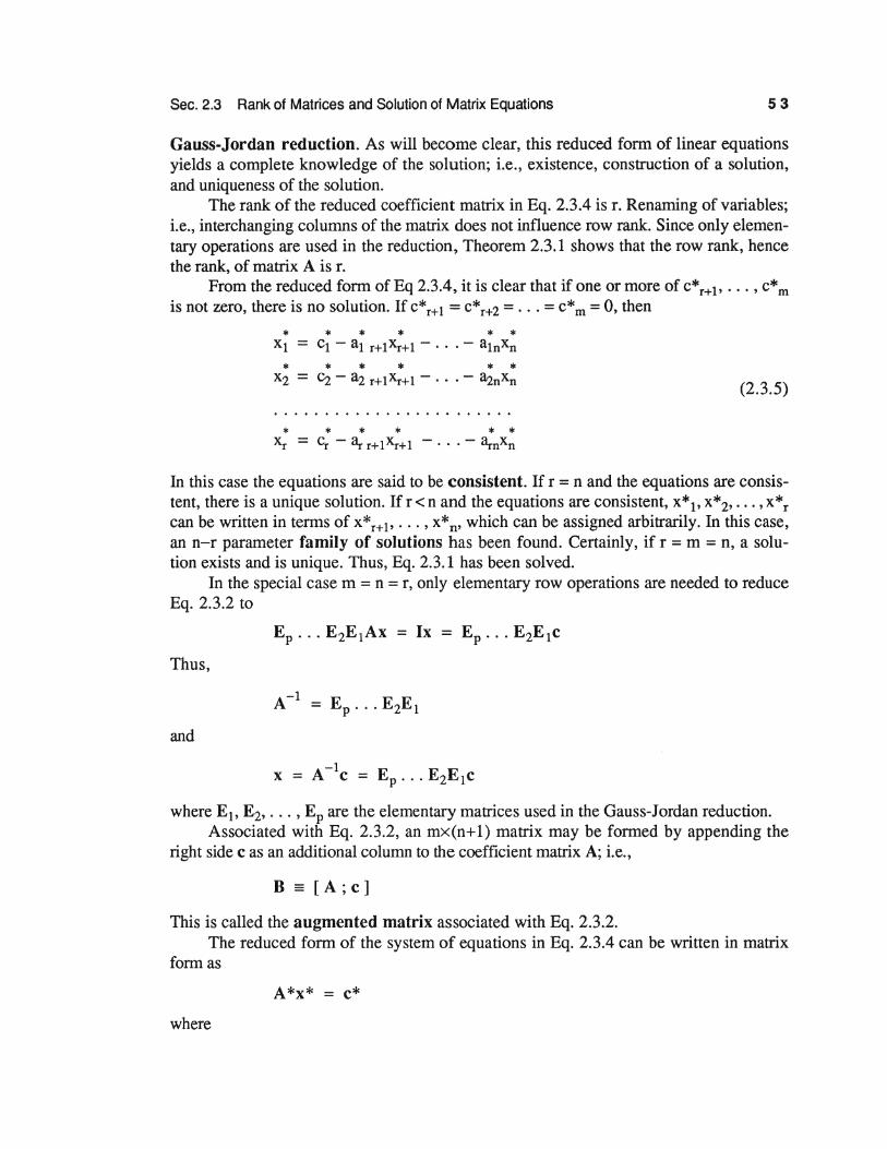
From the reduced form ofEq 2.3.4, it is clear that if one or more of c*r+l• ... , c* m
is not zero, there is no solution. If c* r+ 1 = c* r+2 = ... = c* m = 0, then
* * * * * * X1 = C1- a1 r+1Xr+1- · · ·- a1nxn
* * * * * * X2 = ~- a2 r+1Xr+1- · · ·- a2nXn (2.3.5)
* * * * * * Xr = Cr - 8, r+ 1 Xr+ 1 - · · · - 8rnXn
In this case the equations are said to be consistent. If r = n and the equations are consistent, there is a unique solution. If r <nand the equations are consistent, x*1, x*2, ... , x* r can be written in terms of x*r+l• ... , x* n• which can be assigned arbitrarily. In this case, an n-r parameter family of solutions has been found. Certainly, if r = m = n, a solution exists and is unique. Thus, Eq. 2.3.1 has been solved.
In the special case m = n = r, only elementary row operations are needed to reduce Eq. 2.3.2 to
Thus,
and
x = A - 1c = EP ... E2E 1c
where El> E2, ... , EP are the elementary matrices used in the Gauss-Jordan reduction. Associated with Eq. 2.3.2, an mx(n+l) matrix may be formed by appending the
right side cas an additional column to the coefficient matrix A; i.e.,
B=[A;c]
This is called the augmented matrix associated with Eq. 2.3.2. The reduced form of the system of equations in Eq. 2.3.4 can be written in matrix
form as
A*x* = c*
where
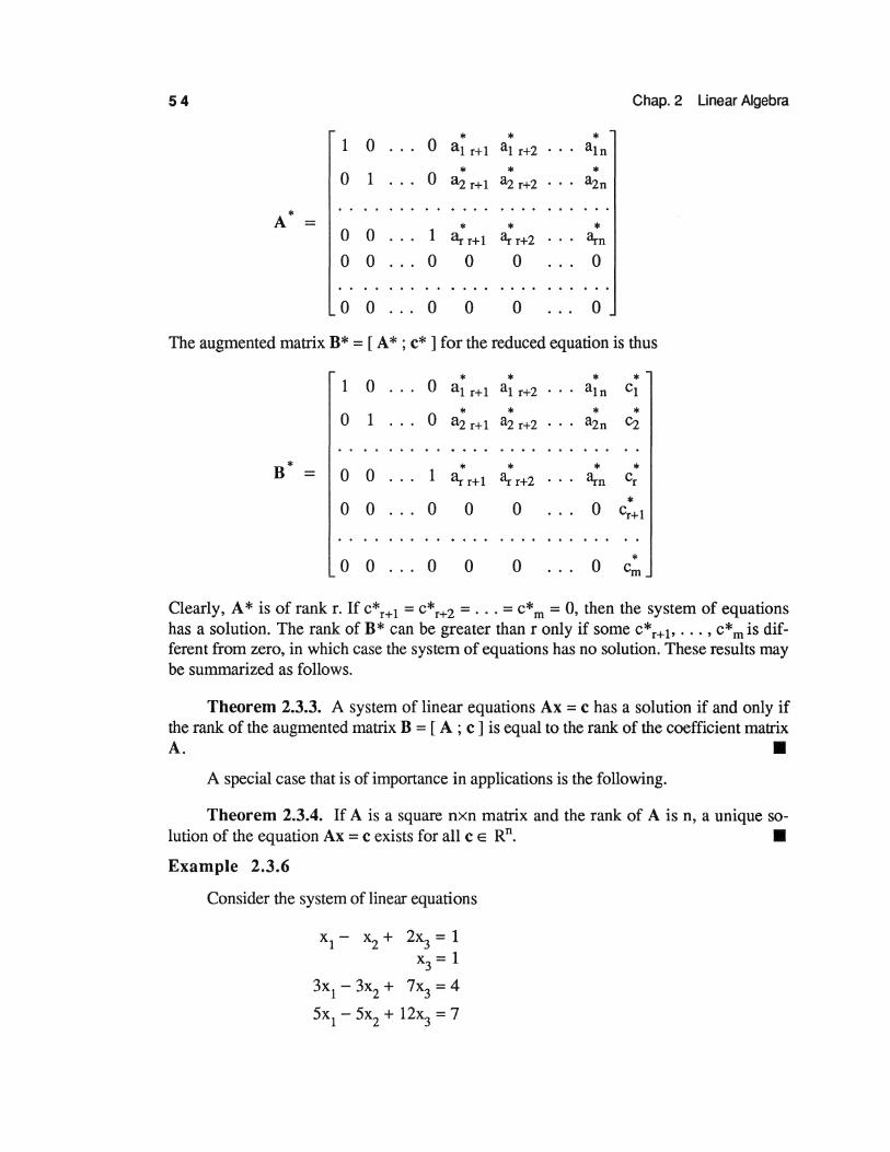
54 Chap. 2 Unear Algebra
0 * * * 1 0 al r+l al r+2 aln
0 * * * 0 1 ~r+l a2 r+2 3zn
A* = * * * 0 0 1 ~r+l 3rr+2 3rn 0 0 0 0 0 0
0 0 0 0 0 0
The augmented matrix B* = [ A* ; c* ] for the reduced equation is thus
0 0 * * * * 1 al r+l al r+2 aln cl
0 0 * * * * 1 a2 r+l a2 r+2 a2n ~
B* 0 0 1 * * * * = ~r+l 3rr+2 3rn Cr
0 0 0 0 0 0 * Cr+l
0 0 0 0 0 0 * Cm
Clearly, A* is of rank r. If c* r+ 1 = c* r+Z = ... = c* m = 0, then the system of equations has a solution. The rank of B* can be greater than r only if some c*r+l• ... , c* m is different from zero, in which case the system of equations has no solution. These results may be summarized as follows.
Theorem 2.3.3. A system of linear equations Ax = c has a solution if and only if the rank of the augmented matrix B = [ A ; c ] is equal to the rank of the coefficient matrix A. •
A special case that is of importance in applications is the following.
Theorem 2.3.4. If A is a square nxn matrix and the rank of A is n, a unique so-lution of the equation Ax = c exists for all c e Rn. •
Example 2.3.6
Consider the system of linear equations
x1 - x2 + 2x3 = 1 x3 = 1
3x1 - 3x2 + 7x3 = 4
5x1 - 5x2 + 12x3 = 7

Sec. 2.3 Rank of Matrices and Solution of Matrix Equations 55
The augmented matrix is
B = [~ ~: ! i] 5 -5 12 7
After Gauss-Jordan reduction,
[ 1 -1 0 -1] B* = 0 0 1 1
0 0 0 0 0 0 0 0
Thus the rank of B is the same as the rank of A and a solution exists. A solution can be determined as x3 = 1 and x1 = x2 - 1, for any value of x2• Thus the solution is not unique. •
Example 2.3. 7
Consider a system of linear equations that is the same as in Example 2.3.6, but with the right side of the third equation changed from 4 to 5. The augmented matrix B in this case is
B = [~ ~: n] 5 -5 12 7
After Gauss-Jordan reduction,
[ 1 -1 0 -1] B* = 0 0 1 1
0 0 0 1 0 0 0 0
Thus, the rank of B is 3, whereas the rank of A is only 2. Theorem 2.3.3 shows that there is no solution to this system of equations. •
It is interesting that only a slight difference in the equations of Examples 2.3.6 and 2.3. 7 leads to drastically different results. In one case there are infinitely many solutions, whereas in the other case there are none.
A case of particular importance is that in which c1 = c2 = ... = cm = 0 in Eq. 2.3.1. In this case, the system of linear equations is homogeneous. Adding a column of zeros to the coefficient matrix cannot affect its rank, so the augmented matrix has the same rank as
56 Chap. 2 Linear Algebra
the coefficient matrix. By Theorem 2.3.3, such a system always has a solution. This is not surprising, since x1 = x2 = ... = Xn = 0 is a solution, called the trivial solution. It is important to know whether a homogeneous system has a nontrivial solution; i.e., a solution in which at least one of the xi is not zero.
Theorem 2.3.5. A system of m homogeneous linear algebraic equations Ax = 0 in n unknowns has a nontrivial solution; i.e., x :1: 0, if m < n. A system of n homogeneous linear algebraic equations in n unknowns has a nontrivial solution if and only if the detenninant of the coefficient matrix is zero; i.e., if the coefficient matrix is singular. •
The proof of this theorem is left as an exercise.
Example 2.3.8
Let the coefficient matrix of a system of two homogeneous equations in three unknowns be, from Example 2.3.5,
A = [4 3 1] 1 2 1
Here, m = 2 and n = 3, so m < n. Thus, a nontrivial solution of Ax= 0 exists as x2 = -3x1, x3 = 5x1, for any x1 # 0.
For a system of three homogeneous linear equations in three unknowns (m = 3, n = 3), let the coefficient matrix be
A = [~ ~ ~] 3 4 2
From Example 2.3.4, A has rank 2. Thus, a nontrivial solution of Ax = 0 exists. Finally, the coefficient matrix A of Example 2.3.1 is
[ 1 1 1] A= 2 0 0
1 2 0
Since I A I = 1 # 0, there is only the trivial solution for Ax = 0. • Deleting some, but not all, of the rows or columns of an mxn matrix yields a sub
matrix of A. A well known result, whose proof may be found in Ref. 1 (p. 98), is the following.
Theorem 2.3.6. The rank of a matrix is the dimension of the largest square sub-matrix with a nonzero determinant. •
Sec. 2.3 Rank of Matrices and Solution of Matrix Equations
Example 2.3.9
For the matrix
A=[~~~~] -1 -3 3 0
57
every 3x3 submatrix has zero determinant. However, deleting the third row and second and fourth columns,
1~ ~ 1 = 9-6 = 3 ~ o
Thus, the rank of A is two. • Example 2.3.10
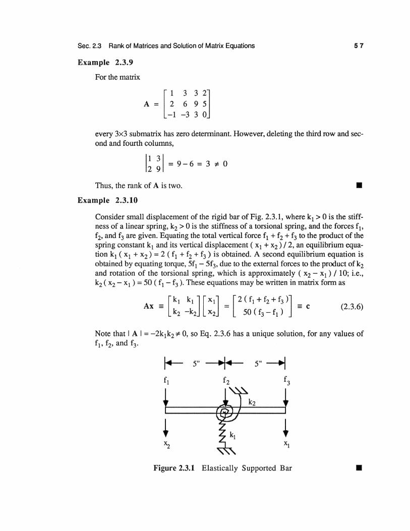
Consider small displacement of the rigid bar of Fig. 2.3.1, where k1 > 0 is the stiffness of a linear spring, k2 > 0 is the stiffness of a torsional spring, and the forces f1,
f2, and f3 are given. Equating the total vertical force f1 + f2 + f3 to the product of the spring constant k1 and its vertical displacement ( x1 + x2 ) I 2, an equilibrium equation k1 ( x1 + x2 ) = 2 ( f1 + f2 + f3 ) is obtained. A second equilibrium equation is obtained by equating torque, 5f1 - 5f3, due to the external forces to the product ofk2 and rotation of the torsional spring, which is approximately ( x2 - x1 ) I 10; i.e., k2 ( x2 - x1 ) =50 ( f1 - f3 ). These equations may be written in matrix form as
(2.3.6)
Note that I A I= -2k1k2 ~ 0, so Eq. 2.3.6 has a unique solution, for any values of f1, f2, and f3•
~ 5" 5"~
Figure 2.3.1 Elastically Supported Bar •
58 Chap. 2 Linear Algebra
EXERCISES 2.3
1. For each of the following matrices. verify Theorem 2.3.2 by determining their row and column ranks:
(a) [~1 ~ ~] 3 1 2
[1 -2 -1] (b) 2 -1 3
7 -8 3
(c) [~ =~ ~1] 7 -8 3 5-7 0
2. Find a solution of the following system of equations:
x1 + x2 + 2x3 = -1 x1 - 2x2 + x3 = -5
3x1 + x2 + x3 = 3
if one exists, by using the Gauss-Jordan Reduction Method.
3. Prove Theorem 2.3.5.
4. Determine if the following system of equations has a solution:
2x1 + x2 - x3 + x4 = -2 x1 - x2 - x3 + x4 = 1 x 1 - 4x2 - 2x3 + 2x4 = 6
4x1 + x2 -4x3 +3x4 =-1
5. Determine the values of A. for which the following system has a nontrivial solution:
9x1 - 3x2 = A.x1 -3x1 + 12x2 - 3x3 = A.x2
- 3x2 + 9x3 = A.x3
Find a nontrivial solution for each of these values of A..
I 6. Find a nontrivial solution of the following system of equations:
x 1 + x2 - x3 + x4 = 0 -x1 + 2x2 + x3 - x4 = 0 2x1 - x2 + 3x3 - 2x4 = 0
7. If xO is a solution of Ax = 0 and x 1 is a solution of Ax = c, show that kxO + x 1 is also a solution of Ax = c, for any value of k. State a criterion for uniqueness of the solution of Ax = c.
8. Consider the matrix
A = [~ ~ ~ ~] 1 0 1 -1
Sec. 2.3 Rank of Matrices and Solution of Matrix Equations
(a) What is the rank of A? (b) Solve the matrix equation Ax= [ 1, 1, 1 ]T. (c) Solve the matrix equation Ax= [ 0, 0, 0 ]T.
9. Consider the system of equatiQns
x1 + 2x2 = 1 x1 - x2 + x3 = 4
3x2 - x3 = c
(a) For what values of c does a solution exist? (b) If a solution exists, is it unique? (c) For values of c for which a solution exists, fmd all solutions.
59
10. For what values of the constant c does the following system of equations have a solution?
[l : m::J = [~J 11. For what values of c1, c2, c3, and c4 does the following system of equations have a
solution:
12. Let A= [ aij lnxn be a symmetric matrix. Show that Ax= 0, x e Rn, has a nontrivial solution if and only if the columns of A are linearly dependent
13. Show that the following equation has a unique solution, without solving the problem numerically:
14. For a given matrix equation Ax= c, let A be an nxm matrix, n > m, with columns aci• i = 1, 2, ... , m, that are linearly independent. Find condition(s) that the vector c e Rn must satisfy so that the matrix equation will have a solution (Hint: write Ax in terms of the acJ
60 Chap. 2 Linear Algebra
2.4 SCALAR PRODUCT AND NORM
The scalar product of two geometric vectors in three dimensional vector analysis was defmed geometrically in Section 2.1 and shown to be
-+ -+ T X . Y = X Y = XtYt + X2Y2 + X3Y3 (2.4.1)
where xi and Yi are Cartesian components of Jt andy. The scalar product can be viewed as a function that assigns to each pair of vectors x and y of R3 a real number. The definition of scalar product can be extended to more general vector spaces by defining it to have the basic properties of the scalar product in R3 from Section 2.1.
Scalar Product on a Vector Space
Definition 2.4.1. Let V be a vector space. A scalar product on V is a real valued function ( • , • ) of pairs of vectors in V with the following properties:
(1) (X, y) = ( y, X) (2) ( X, y + Z ) = ( X, y ) + ( X, Z )
(3) ( ax, y ) = a ( x, y ) (4) (X, X) ;::: 0 (5) ( x, x ) = 0, if and only if x = 0
for any vectors x, y, and z in V and any real scalar a.
(2.4.2)
• Note that the scalar product in Eq. 2.4.1 has all the basic properties of the usual
scalar product in R3. A natural generalization of this scalar product to Rn is
(2.4.3)
Example 2.4.1
The product of Eq. 2.4.3 is not the only scalar product in Rn; e.g, let x = [ x1, x2 ]T
andy= [ y1, y2 ]T be in R2. Define
Then, [ x, x] = x12 - 2x1x2 + 2xl = ( x1 - x2 )2 + x22 > 0 if x '# 0. The remaining properties of Definition 2.4.1 can also be verified, which is left as an exercise. Hence [ •, •] is also a scalar product on R2. •
Norm and Distance in a Vector Space
Recall that, in three dimensional vector analysis, the scalar product of a vector with itself is the square of the length of the vector. Using this concept, the length of a vector may be extended to a general vector space.
Sec. 2.4 Scalar Product and Norm 61
Definition 2.4.2. The norm of a vector in a vector space V that has a scalar product ( • , • ) is
llxii::...J(x,x)
Example 2.4.2
(2.4.4)
• Find the norm and length of the vector x = [ 1, 2, 3 ]Tin R3• The norm of xis defined in Eq. 2.4.4 as
The length of t is
~
lxl= rx:x:=-fii "'/ AiAi
Therefore, II x II is the length of x. • The norm has most of the properties that are usually associated with length or dis
tance. From the postulates for scalar product in Definition 2.4.1,
llxll;;::: 0 II x II = 0, if and only ifx = 0 llaxll =lalllxll
(2.4.5)
Note that a different scalar product will give a different norm and hence one vector space may have many different norms. Thus, the concept of distance in a general vector space is dependent on the norm used. This might be considered as analogous to using different units of length in the physical world. Unfortunately general norms are not proportional to one another, so there is not a simple scale conversion factor that relates norms.
Theorem 2.4.1 (Schwartz Inequality). For any vectors x and y in a vector space V with scalar product ( • , • ) and associated norm II • II defined by Eq. 2.4.4,
l<x.y)l:::; llxllllyll
To prove Theorem 2.4.1, let a be any scalar and form
0 :::; II x + ay 112 = ( x + ay, x + ay ) = ( x, x ) + ( ay, x ) + ( x, ay ) + ( ay, ay ) = II x 112 + a ( y, x ) + a ( x, y ) + a2 II y 112
(2.4.6)
•
62 Chap. 2 Linear Algebra
This can be written as
0 s II x 112 + 2a ( x, y) + a2 II y 112 == g(a)
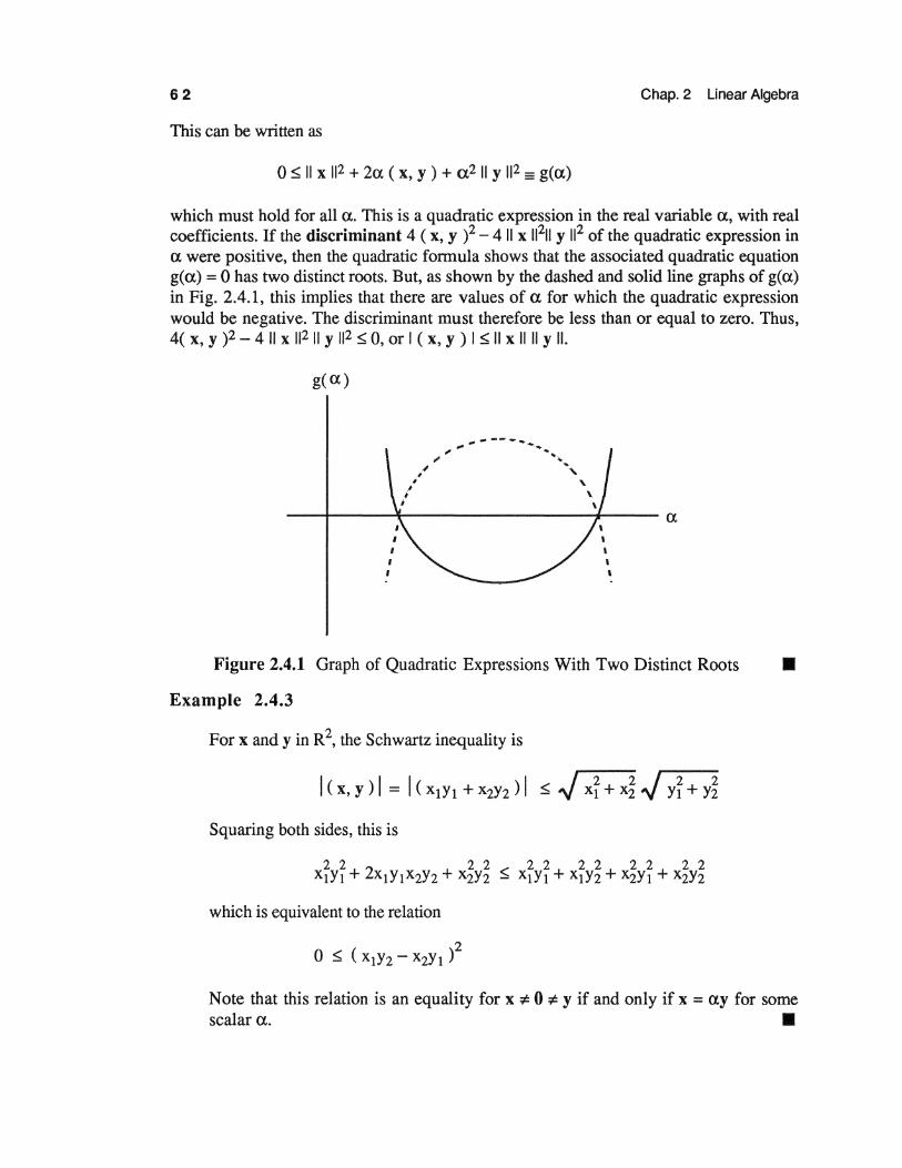
which must hold for all a. This is a quadratic expression in the real variable a, with real coefficients. If the discriminant 4 ( x, y )2 - 4 II x 11211 y 112 of the quadratic expression in a were positive, then the quadratic formula shows that the associated quadratic equation g(a) = 0 has two distinct roots. But, as shown by the dashed and solid line graphs of g(a) in Fig. 2.4.1, this implies that there are values of a for which the quadratic expression would be negative. The discriminant must therefore be less than or equal to zero. Thus, 4( x, y )2 - 4 II x 112 II y 112 S 0, or I ( x, y ) I S II x II II y II.
g(a)
Figure 2.4.1 Graph of Quadratic Expressions With Two Distinct Roots •
Example 2.4.3
For x andy in R2, the Schwartz inequality is
Squaring both sides, this is
22 22 22 22 22 22 XtYt + 2x1Y1X2Y2 + X2Y2 S XtYt + X1Y2 + X2Y1 + X2Y2
which is equivalent to the relation
Note that this relation is an equality for x :i: 0 :i: y if and only if x = ay for some ~ar~ •
Sec. 2.4 Scalar Product and Norm 63
The Schwartz inequality for the vector space Rn, with the scalar product defined in Eq. 2.4.3, is
( n Jl/2 ( n Jl/2
1 < x. y > 1 = 1 XiYi 1 ~ fr x?- fr Yr = 11 x 1111 y 11 (2.4.7)
The Schwartz inequality leads to another important inequality.
Theorem 2.4.2 (Triangle Inequality). For any vectors x and y in a vector space V that has a scalar product ( • , • ) and associated norm II • II defined by Eq. 2.4.4,
llx+yll~llxll+llyll
To prove Theorem 2.4.2, note that
II X + y 112 = ( X + y' X + y ) = II X 112 + II y 112 + ( x, y ) + ( y' X )
~ II X 112 + II y 112 + 2 I ( X, y ) I ~ II X 112 + II y 112 + 2 II X II II y II = (llxll+llyll)2
where the Schwartz inequality has been used. Thus, Eq. 2.4.8 follows.
(2.4.8)
•
• In a vector space V, a vector is sometimes referred to as a point. The distance
between two points in V is then defined as the norm of the difference of the vectors; I.e.,
d ( X, y ) = II X - y II (2.4.9)
This definition of distance satisfies all the usual properties associated with distance in R3;
i.e., for any x, y, and z in V,
(1) the distance between two points is positive unless the points coincide; i.e.,
d ( X, y ) = II X - y II ~ 0 d ( x, y) =II x- y II= 0, if and only if x = y
(2) the distance function is symmetric; i.e.,
d ( X, y ) = II X - y II = II y - X II = d ( y' X )
(3) the triangle inequality is satisfied; i.e.,
d ( X, y ) = II X - y II ~ II X - z II + II z - y II = d ( X, z ) + d ( z, y )

64 Chap. 2 Linear Algebra
A vector space in which distance between points is defined with the above three properties is called a metric space and the distance function d ( • , • ) is called a metric. These ideas justify the use of II x - y II as a distance.
Orthonormal Bases
It has already been seen that there are many bases in an n-dimensional vector space, all of which are sets of n linearly independent vectors that span the space. If a scalar product is defmed, certain bases with special properties that are useful in analysis and computation can be defmed.
Definition 2.4.3. Two vectors are orthogonal if their scalar product is zero. A vector is said to be normalized if its norm is one. A set of vectors xl, x2, ... , xn is orthonormal if
where B .. is the Kronecker delta of Definition 1.2.3. lJ
(2.4.10)
• Let { xi } be a set of n orthonormal vectors that span an n-dimensional vector space
V. They must be linearly independent, since if ~xi = 0, taking the scalar product of both sides with x.i yields
0 = ( xj, 0 ) = ( xj, aixi) = aiBij = aj
Hence, aj = 0 for all j and the set { xi } is linearly independent. Therefore, the set of vectors { xi } is a basis for V.
Having an orthonormal basis is very convenient for computation, because the representation of any vector in the space is easy to find. Suppose x is a vector in V with the representation
(2.4.11)
in terms of an orthonormal basis { xi } . Taking the scalar product of both sides with x.i,
( xj, x ) = ai ( xj, xi )
= ~Bji = aj (2.4.12)
Thus, the components~ of the vector a= [ a1, •.• , Rn ]Tin Rn that represents x are easily determined. Consider another vector yin V, with the representation
y = bjxj
where b = [ b1, ... , bn ]T represents y. The scalar product of x andy in Vis

Sec. 2.4 Scalar Product and Norm 65
(X, y) = (~xi, bjxj)
= aibj ( xi, xj )
= ~b·O·· J lj
= ~bi
These relations establish a one-to-one correspondence between the n-dimensional vector space V and the coefficients of Eq. 2.4.11 in the space Rn, since the scalar product in Rn for a pair of vectors a= [ a1, a2, .•. , ~ ]T and b = [ b1, b2, ••. , bn ]Tis ~bi. Furthermore, under this correspondence, scalar product is preserved; i.e.,
(2.4.13)
Consider now the possibility of changing the representation of a vector space V by a change of basis. Let { xi } and { yi } be two bases for the same vector space. Then, any vector win Rn has a representation in terms of each basis; i.e.,
w = b·xi 1 (2.4.14)
(2.4.15)
Each vector xi in the basis { xi } has a representation in terms of the { yi } , denoted as
xj = a··yi 1J
Substituting this relation into Eq. 2.4.14 and using Eq. 2.4.15,
w = c-yi = b·xj = b·a··yi = a··b·yi 1 J J 1J 1J J
Since the representation of a vector in terms of a given basis is unique,
C· =a··b· 1 1J J
(2.4.16)
(2.4.17)
Let b be the column matrix with element bi, c be the column matrix with elements ci, and A be the square matrix with elements ~j· Then, the change of representation of Eq. 2.4.17 can be written in matrix form as
c=Ab (2.4.18)
Thus, the change in coefficients of a vector in V, associated with a change in basis, is defmed by a matrix transformation.
Consider the important special case of a change from one orthonormal basis { xi } to another orthonormal basis { yi }. Taking the scalar product of both sides of Eq. 2.4.16 with xi and using Eq. 2.4.16,

66
Oij = (xi, xj) = ( akiyk, 8mjYm)
= aki~ ( yk, ym) = aki~j~m = akiakj
T = aikakj
Chap. 2 Linear Algebra
In terms of operations with the matrix A= [ ~j ], this is
(A )T A= I (2.4.19)
Thus,
A-1 =AT (2.4.20)
Definition 2.4.4. A matrix A for which A - 1 = AT is called an orthogonal matrix. •
Example 2.4.4
Find the transformation matrix A between the orthonormal bases
y1 = [ 1, 0, 0 ]T, l = [ 0, 1, 0 ]T, y3 = [ 0, 0, 1 ]T
and
1 1 T 21 T 3 1 T X = '13[ 1, 1,1] , X = 12[-1, 1, 0] , X = "6 [-1,-1,2]
It is easy to write the xi in terms of the yi as
1 1 1 2 3 X = .V3 ( y + y + y )
2 1 1 2 X = .V2 (- y + y )
3 1 1 2 3 X = " 6 ( - y - y + 2y )
Thus, the matrix A= [a .. ] defined in Eq. 2.4.16, in this case, is lJ
1 1 1 {3 .V3 .V3
1 1 0 A=
.V2 .V2
Direct manipulation verifies that AT A = I. •

Sec. 2.4 Scalar Product and Norm 67
Example 2.4.5
A rotation of the x1 - x2 plane in R3 about the xraxis through an angle 9, as shown in Fig. 2.4.2, can be viewed as the orthogonal transformation; i.e.,
where x1', x2', and x3' are components of the vector x in the x1'-x2'-x3' frame. Using trigonometric identities,
0
29 . 29 cos + sm 0
.... 9
x' ... 1
~] = I
Figure 2.4.2 Rotation of the x1-x2 Plane About the xrAxis •
One of the important properties of an orthogonal transformation is that it leaves the scalar product invariant. That is, if x =Ax' andy= Ay', x' = ATx andy'= ATy, and
( x', y' ) = ( AT x ) T AT y = x T AA T y = X Tly = ( x, y )
Further, the orthogonal transformation is norm preserving; i.e.,
II x' II = ( x', x' )1/2 = ( x, x )112 = II x II
(2.4.21)
Since the angle between two vectors is given by cos 9 = ( x, y ) I ( II x II II y II ), an orthogonal transformation is also angle preserving.
The scalar product can be used to obtain an analytical criterion for linear dependence of a set of m vectors { x 1, x2, •.. xm } in a vector space V. Set a linear combination of the xi to zero, as in Eq. 2.2.1, to check for linear independence; i.e., cixi = 0. By succes-

68 Chap. 2 Linear Algebra
sively forming the scalar products of x1, •.. , xm with both sides, the constants ci must satisfy
c1 ( x 1 , x1 ) + c2 ( x1 , x2 ) + ... + cm ( x1 , xm) = 0
c1 ( x2 , x1 ) + c2 ( x2 , x2 ) + ... + cm ( x2 , xm ) = 0 (2.4.22)
This system of equations inc= [ c1, •.. , cm ]T can be written in matrix form as
Gc=O (2.4.23)
where the mxm matrix G is called the Gram matrix of { x1, ••• , xm } , defined as
( xl 'xl ) ( xl , x2) ( xl 'xm)
G= ( x2 , xl ) ( x2, x2) ( x2 'xm)
(2.4.24)
( xm 'xl) ( xm 'x2) ( xm 'xm)
The set of m equations in the m variables ci in Eq. 2.4.23 has a nontrivial solution if and only if the determinant of the matrix of coefficients vanishes; i.e.,
IGI=O (2.4.25)
The determinant I G I is called the Gram Determinant, or Gramian, of { xl, ... , xm } . This result may be stated in terms of linear dependence of the xi as follows.
Theorem 2.4.3. A set of vectors in a vector space V that has a scalar product ( • , • ) is linearly dependent if and only if its Gramian is zero. Conversely, they are linearly independent if and only if their Gramian is not zero. •
Example 2.4.6
Use Theorem 2.4.3 to determine whether the following vectors in R4 are linearly dependent:
xl = [ 1, 1, 1, 0 ]T, x2 = [ 1, -1, 0, 0 ]T, x3 = [ 0, 0, 1, 1 ]T
The Gramian of these vectors is
3 0 1 I G I = 0 2 0 = 12 - 2 = 10 :#= 0
1 0 2
Therefore, x1, x2, and x3 are linearly independent. •

Sec. 2.4 Scalar Product and Norm 69
Consider a basis { x1, ... , xm } of a vector space V that may not be orthogonal. If xis a vector in V, it can be written as a linear combination of the xi; i.e.,
(2.4.26)
Taking the scalar product of both sides with xi, i = 1, 2, ... , m, yields
or, in matrix form,
Ga = [ ( x 1, x ), ... , ( xm, x ) ]T = b (2.4.27)
Thus, finding the expansion of a vector in terms of a basis of V requires the solution of a matrix equation, Eq. 2.4.27, whose coefficient matrix is the Gram matrix. By Theorem 2.4.3, G is nonsingular, so a unique solution exists.
Note that if the basis { xi } is orthonormal, (xi, xj) = Bij and the Gram matrix is the identity; i.e., G =I. In this very special case, Eq. 2.4.27 reduces to ai = (xi, x ), which is the same as Eq. 2.4.12. The value of having an orthonormal basis thus becomes clear.
Gram-Schmidt Orthonormalization
As noted earlier, orthonormal bases have very attractive properties. It is now to be shown that from any n linearly independent vectors that span a vector space V, an orthonormal basis can be constructed. Let { f } be a basis whose vectors are not necessarily orthonormal. First normalize y1, to obtain
1 1 1 X= -y
II y1 11
Next, form x2 = a21 x1 + a22y2 and choose a21 and a22 so that ( x1, x2 ) = 0 and II x2 11 = 1. This leads to two equations for a21 and a22• The result is
a21 = -a22 ( x 1 ' y2 )
Thus,
2 [ 2 ( 1 2) 1] X = a22 y - X , y X
By mathematical induction, continue constructing an orthonormal set of vectors xl, x2, ... , xa, a ~ n, where
70 Chap. 2 Linear Algebra
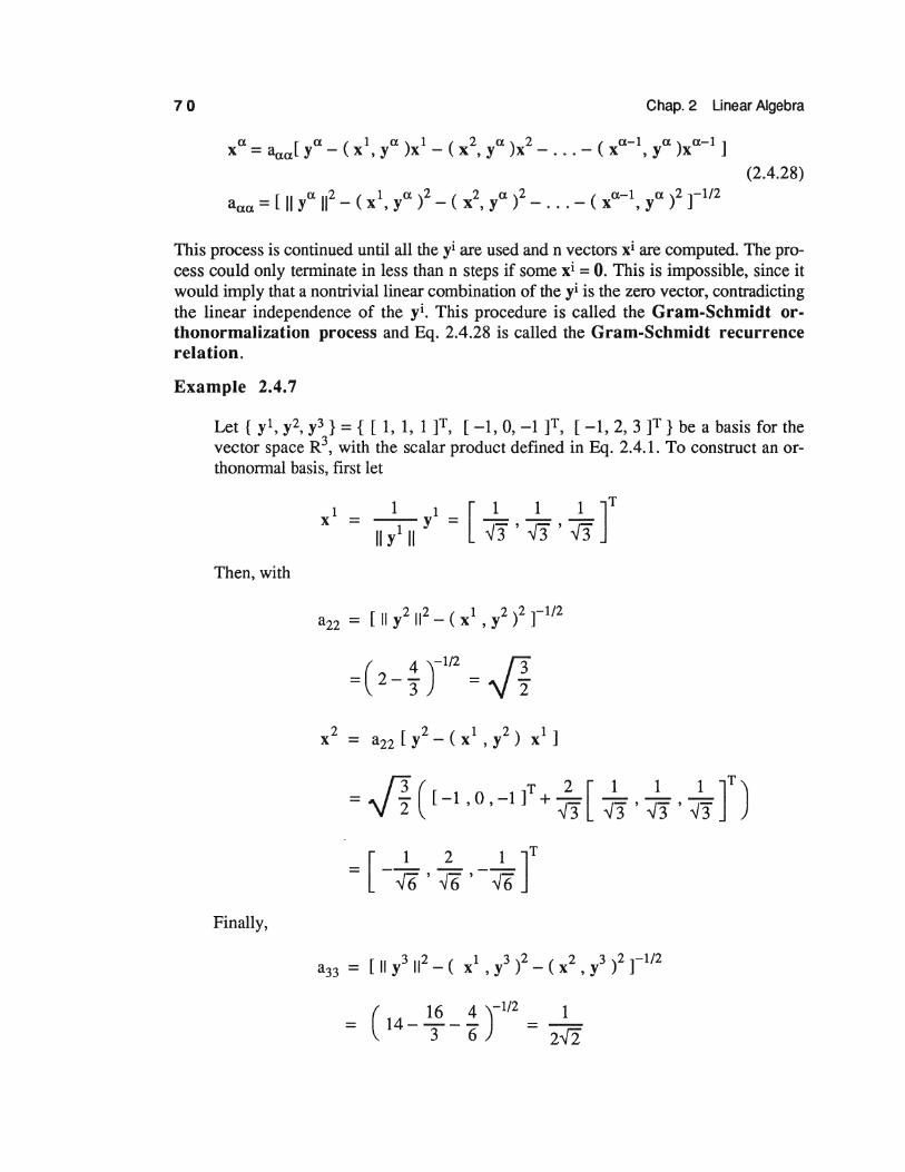
a [ a ( 1 a ) 1 ( 2 a ) 2 ( a-1 a ) a-1 ] X = aua y - X , y X - X , y X - ... - X , y X (2.4.28)
= [ II a ll2 _ ( 1 a )2 _ ( 2 a )2 _ _ ( a-1 a )2 1-1/2 aaa y X ,y x ,y . . . x ,y
This process is continued until all the yi are used and n vectors xi are computed. The process could only terminate in less than n steps if some xi = 0. This is impossible, since it would imply that a nontrivial linear combination of the yi is the zero vector, contradicting the linear independence of the yi. This procedure is called the Gram-Schmidt orthonormalization process and Eq. 2.4.28 is called the Gram-Schmidt recurrence relation.
Example 2.4. 7
Let { y1, y2, y3} = { [ 1, 1, 1 ]T, [ -1, 0, -1 ]T, [ -1, 2, 3 F} be a basis for the vector space R3, with the scalar product defined in Eq. 2.4.1. To construct an orthonormal basis, first let
1 1 1 [ 1 1 1 JT X = ii7ii y = "J3 ' V3 '{3
Then, with
/3 ( T 2 [ 1 1 1 JT ) = V 2 [ - 1 • 0 • - 1 1 + -:r3 v3 • v3 • "J3
Finally,

Sec. 2.4 Scalar Product and Norm 71
3 [ 3 ( 1 3) 1 ( 2 3) 2] X = a33 Y - X , y X - X , y X
1 ( T 4 [ 1 1 1 ]T = 2f2 [ -1 ' 2 ' 3 ] - {3 {3 ' {3 ' 13
2 [ 1 2 1 JT) - {6 -16' {6 ,-{6
= [ -:z.o.:zr • A final result associated with the scalar product that is of great theoretical and com
putational importance is the following.
Theorem 2.4.4. Let xi, i = 1, ... , n, be a set of linearly independent vectors in an n-dimensional vector space V with scalar product ( • , • ). Then, the only vector in V that is orthogonal to each of these vectors is the zero vector. •
To prove Theorem 2.4.4, let y be a vector in V such that
(xi, y ) = 0, i = 1, ... , n (2.4.29)
Since the xi are linearly independent, they form a basis for V. Thus, there is a unique set of constants ai, i = 1, ... , n, such that
(2.4.30)
Substituting Eq. 2.4.30 into Eq. 2.4.29,
(xi, a.xj) = (xi, xj) a. = 0, i = 1, ... , n J J
(2.4.31)
The coefficient matrix in Eq. 2.4.31 is the Gram matrix of the linearly independent vectors xi, i = 1, ... , n, so it has rank n. Therefore, aj = 0, i = 1, ... , n. But, from Eq. 2.4.30, y = 0, which was to be shown. •
Example 2.4.8
The vectors x1 = [ 1, 1, 1 ]T, x2 = [ 1, -1, 0 ]T, and x3= [ 0, 0, 1 ]T are linearly independent. Let y be a vector in R3• Then, y is orthogonal to x1, x2, and x3 if
( xl, y) = Yt + y2 + y3 = 0
( x2 • y ) = y 1 - y 2 = 0
( x3 • y ) = y3 = 0
72 Chap. 2 Linear Algebra
The only solution, consistent with Theorem 2.4.4, is
• EXERCISES 2.4
1. Verify that the scalar product of Example 2.4.1 satisfies the properties of Definition 2.4.1.
2. Prove the following statements for a vector space with a scalar product: (a) The Parallelogram rule
II X + y 112 + II X - y 112 = 2 II X 112 + 2 II y 112 (b) The Pythagorean rule
II X + y 112 = II X 112 + II y 112' if ( X, y ) = 0 (c) II x- y II ~Ill x II- II y Ill
3. Show that the Schwartz inequality is an equality if and only if the vectors x andy are proportional; i.e., y =ax for some scalar a.
4. Show that the triangle inequality is an equality if and only if the two vectors x and y are proportional and the constant of proportionality is a nonnegative real number.
5. Test the following set of vectors for linear independence and construct from it an orthonormal basis for R4: [ 1, 0, 1, 0 ]T, [ 1, -1, 0, 1 ]T, [ 0, 1, -1, 1 ]T, [ 1, -1, 1,-1 ]T.
6. (a) Let x, y, and z be vectors in R3, such that x andy are orthogonal and x and z are orthogonal. Prove that x and any vector in R3 of the form ay + bz, where a and bare real numbers, (that is, a linear combination of y and z) are orthogonal.
(b) Let x be a vector in R3. Prove that the set of all vectors yin R3 such that x and y are orthogonal is a subspace of R3.
7. Prove that if xis in R3 and ( x, y) = 0 for ally in R3, then x = 0.
8. Show that the matrix equation
Ax = [ ~ ~ ~ 1] [ ::] = [ i] = c 3 3 -5 x3 1
possesses a one-parameter family of solutions and verify directly that the vector c is orthogonal to all solutions of AT y = 0.
Sec. 2.4 Scalar Product and Norm 73
9. Show that if A and B are orthogonal nxn matrices, then A TB is an orthogonal matrix.
10. If A is an orthogonal nxn matrix and c e Rn, solve AAx = c for x. Find the solution in terms of AT.
11. In R3, find all vectors that are orthogonal to both [ 1, 1, 1 ]T and [ 1, -1, 0 ]r. Produce, from these vectors, a mutually orthogonal system of unit vectors; i.e., an orthonormal basis for R3•
12. If u is a unit vector, show that Q =I- 2uuT is an orthogonal matrix, known as a Householder transformation. Compute Q explicitly when u = (1!-v3)[ 1, 1, 1 ]r.
13. Show that x - y is orthogonal to x + y if and only if II x II = II y II.