downloads.hindawi.comdownloads.hindawi.com/journals/ijdsn/2011/980953.pdf2 International Journal ofDistributed Sensor Networks Interfering access point’s coverage Interfering access

Hindawi Publishing CorporationInternational Journal of Distributed Sensor NetworksVolume 2011, Article ID 980953, 17 pagesdoi:10.1155/2011/980953

Research Article

Low-Complexity, Distributed Characterization ofInterferers in Wireless Networks

Vibhav Kapnadak,1 Murat Senel,2 and Edward J. Coyle3

1 Network Systems Engineering, AT&T Labs, 2600 Camino Ramon, CA 94583, USA2 Robert Bosch LLC, Research and Technology Center North America, 4009 Miranda Avenue, Palo Alto, CA 94304, USA3 School of Electrical and Computer Engineering, Georgia Institute of Technology, 777 Atlantic Drive NW, Atlanta,GA 30332-0250, USA

Correspondence should be addressed to Edward J. Coyle, [email protected]

Received 8 February 2011; Revised 21 May 2011; Accepted 25 May 2011

Copyright © 2011 Vibhav Kapnadak et al. This is an open access article distributed under the Creative Commons AttributionLicense, which permits unrestricted use, distribution, and reproduction in any medium, provided the original work is properlycited.

We consider a large-scale wireless network that uses sensors along its edge to estimate the characteristics of interference fromneighboring networks or devices. Each sensor makes a noisy measurement of the received signal strength (RSS) from an interferer,compares its measurement to a threshold, and then transmits the resulting bit to a cluster head (CH) over a noisy communicationchannel. The CH computes the maximum likelihood estimate (MLE) of the distance to the interferer using these noise-corruptedbits. We propose and justify a low-complexity threshold design technique in which the sensors use nonidentical thresholds togenerate their bits. This produces a dithering effect that provides better performance than previous techniques that use differentnon-identical thresholds or the case in which all the sensor motes use an identical non-optimal threshold. Our proposed techniqueis also shown (a) to be of low complexity compared to previous non-identical threshold approaches and (b) to provide performancethat is very close to that obtained when all sensors use the identical, but unknown, optimal threshold. We derive the Cramer-Raobound (CRB) and also show that the MLE using our dithered thresholds is asymptotically both efficient and consistent. Simulationsare used to verify these theoretical results.

1. Introduction

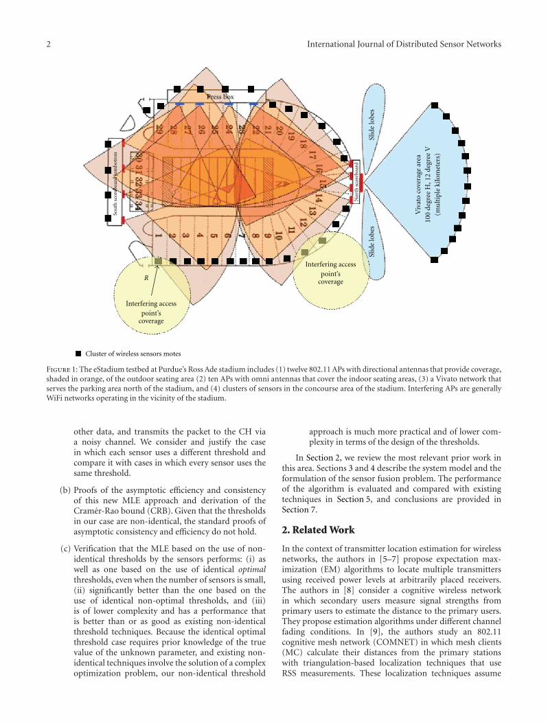
Large-scale deployments of wireless LANs in unlicensed RFbands are often subject to interference from many sources.We have encountered this problem in the e-Stadium wirelesstestbed [1], which enables football fans in the stadium atPurdue to access multimedia content related to the game [2]via 802.11b and 3G networks. The locations and coverageareas of the 802.11b access points (APs) in the stadium areshown in Figure 1. The two interfering APs also shown in thefigure may disrupt eStadium services for fans sitting alongthe outer edge of the stands or in the tailgating area northof the stadium. The locations and settings of these interferingaccess points or devices change over time. The eStadium test-bed must sense these changes and adapt its channel assign-ments and power levels to ensure that its users experiencesatisfactory Quality of Service (QoS).

The eStadium testbed includes clusters of wireless sensorsthat are distributed along the concourse area of the stadium[3]. They currently gather and process information from this

area and make it available to fans and security personnelduring games. We propose that these sensors perform theadditional task of characterizing the sources of interferencewith the 802.11b-based portion of the eStadium testbed.

The information gathered about interferers by these sen-sors is not directly available to the eStadium APs becauseof their directional antennas or shadowing by the stadium’sstructure. A Smart WiFi system [4] would thus not be able tosense and adjust to the presence of these external interferers.This proposed use of the sensors, combined with algorithmsto alter the 802.11b channel assignments and power settings,is thus a cognitive networking approach to enabling thecoexistence of many systems in unlicensed bands.

The contributions of this paper include the following.

(a) Analysis and improvement of MLE approaches inwhich sensors conserve energy by minimizing theamount of data they transmit. Each sensor thresholdsits noisy measurement of the interferer’s signalstrength, adds the resulting bit to a packet carrying

2 International Journal of Distributed Sensor Networks

Interfering accesspoint’s

coverage

Interfering accesspoint’s

coverageR

Slid

elo

bes

Slid

elo

bes

Viv

ato

cove

rage

area

100

degr

eeH

,12

degr

eeV

(mu

ltip

leki

lom

eter

s)

Press box

Nor

thsc

oreb

oard

Sou

t hsc

oreb

oard

jum

botr

on

Cluster of wireless sensors motes

Figure 1: The eStadium testbed at Purdue’s Ross Ade stadium includes (1) twelve 802.11 APs with directional antennas that provide coverage,shaded in orange, of the outdoor seating area (2) ten APs with omni antennas that cover the indoor seating areas, (3) a Vivato network thatserves the parking area north of the stadium, and (4) clusters of sensors in the concourse area of the stadium. Interfering APs are generallyWiFi networks operating in the vicinity of the stadium.

other data, and transmits the packet to the CH viaa noisy channel. We consider and justify the casein which each sensor uses a different threshold andcompare it with cases in which every sensor uses thesame threshold.

(b) Proofs of the asymptotic efficiency and consistencyof this new MLE approach and derivation of theCramer-Rao bound (CRB). Given that the thresholdsin our case are non-identical, the standard proofs ofasymptotic consistency and efficiency do not hold.

(c) Verification that the MLE based on the use of non-identical thresholds by the sensors performs: (i) aswell as one based on the use of identical optimalthresholds, even when the number of sensors is small,(ii) significantly better than the one based on theuse of identical non-optimal thresholds, and (iii)is of lower complexity and has a performance thatis better than or as good as existing non-identicalthreshold techniques. Because the identical optimalthreshold case requires prior knowledge of the truevalue of the unknown parameter, and existing non-identical techniques involve the solution of a complexoptimization problem, our non-identical threshold

approach is much more practical and of lower com-plexity in terms of the design of the thresholds.

In Section 2, we review the most relevant prior work inthis area. Sections 3 and 4 describe the system model and theformulation of the sensor fusion problem. The performanceof the algorithm is evaluated and compared with existingtechniques in Section 5, and conclusions are provided inSection 7.

2. Related Work

In the context of transmitter location estimation for wirelessnetworks, the authors in [5–7] propose expectation max-imization (EM) algorithms to locate multiple transmittersusing received power levels at arbitrarily placed receivers.The authors in [8] consider a cognitive wireless networkin which secondary users measure signal strengths fromprimary users to estimate the distance to the primary users.They propose estimation algorithms under different channelfading conditions. In [9], the authors study an 802.11cognitive mesh network (COMNET) in which mesh clients(MC) calculate their distances from the primary stationswith triangulation-based localization techniques that useRSS measurements. These localization techniques assume

International Journal of Distributed Sensor Networks 3

that the MCs are synchronized and that they are located onthe edge of the secondary 802.11 network; otherwise, theymay not be able to detect the interference from the primarystations. In the above papers, the authors do not considerthe use of thresholded measurements or the transmission ofmeasurements over noisy channels.

In the context of distributed estimation in wireless sensornetworks, the authors in [10, 11] consider 1-bit quantizationusing identical and non-identical thresholds and obtain themaximum-likelihood estimate of an unknown parameter.They account for measurement noise that is Gaussian or hasan unknown distribution but do not consider other sourcesof error, such as noise in the communication channel. A sim-ilar situation is examined in [12], where multiple-bit quan-tized information is used to locate a target in a sensor fieldunder error-free channel conditions. A nonparametric ap-proach to density estimation using a sensor network was in-troduced in [13]. The authors considered the case where 1-bit quantized data is transmitted to the CH using randomthresholds from a pmf. As with the previous papers, however,processing by sensors and the wireless channel between thesensors and the CH are considered to be error free, which istypically not the case in realistic situations. In [14], the au-thors study channel aware target localization using 1-bitquantized data. They analyze the effects on the root meansquared error (RMSE) of the MLE due to communicationchannel impairments. They consider the BSC, Rayleigh fad-ing with coherent reception and non-coherent reception.However, in their work, they do not address the design ofthe 1-bit quantization algorithm for transmission over noisycommunication channels.

In [15, 16], the authors consider a 1-bit quantizationframework for noisy Gaussian communication links. How-ever, it is assumed that either all sensors use the samethreshold or use one of two thresholds. More recently, in[17], the authors have proposed an MLE-based distributedestimation algorithm using 1-bit quantized data that is trans-mitted over a BSC. The context in which the estimation algo-rithm is analyzed is for secure data transmission in wirelesssensor networks, but it is assumed that all the sensors useidentical thresholds.

Several other papers, including [18–21], also study thedistributed estimation problem, but their approach is basedon the best linear unbiased estimate (BLUE) at the CH in-stead of the MLE. This approach is typically not appropriateor optimal when the received data at the CH is a nonlinearfunction of the unknown parameter.

Our approach is unique because it (a) exploits and justi-fies the use of different thresholds by the sensors when quant-izing their noisy measurements and (b) accounts for noisymeasurements by the sensors and error-prone processingand communications between the sensors and the CH. Ouranalysis of the MLE in this new approach will show thatuniformly-spaced thresholds produces a dithering effect thatleads to near-optimal performance when the only informa-tion available about the parameter being estimated is its sup-port. This is very important because previous approachesbased on the use of an identical threshold by all sensors workwell only when the chosen threshold is either very near the

unknown true value, or the number of sensors is very large.Furthermore, our non-identical threshold design algorithmis significantly less complex and performs as good as or betterthan existing non-identical threshold techniques, such as theone in [10].

3. System Model and Problem Motivation

3.1. System Characteristics and Considerations. The followingcharacteristics of the wireless sensor network and sensorfusion algorithm are assumed in this paper. They aremotivated by the eStadium project but are relevant to manyother systems operating in unlicensed bands.

(a) Architecture. The system consists of a network of wirelessAPs and a single-hop cluster of N spatially distributedwireless sensors deployed along the edge of the wirelessnetwork. Each sensor measures the RSS from an interferingAP, compares it to its threshold, and relays the resulting bitto the CH. The CH fuses the bits it receives to produce anestimate of the signal strength and distance to the interferingAP.

(b) Measurement Errors. Due to large-scale fading andshadowing effects, the RSS X(k) observed at sensor k isassumed to be log normally distributed, as in [22, 23]. Themean μ(R) of this distribution is a function of the distance Rfrom the transmitter to the receiver while the variance σ2 isindependent of R. We assume that μ(R) follows a path-loss-exponent model; hence,

μ(R) = K − 10α log(R), (1)

where α is the propagation law exponent, and K is theclose-in reference power, that is, the power very close to thetransmitter. In rest of the paper, the symbol μ will be usedinterchangeably with μ(R). On a dB scale, the received RSS atthe sensors can be expressed as

Xk = μ(R) + nk , k = 1 · · ·N , (2)

where μ(R) is the mean and nk ∼ N (0, σ2n) is i.i.d. Gaussian

noise that is independent of μ. The term σn is commonlyreferred to as the dB spread of the log-normal shadowingand is typically between 4 dB and 12 dB. We refer to thisnoise as the measurement noise because it corrupts the SNRmeasurement of each sensor, and we assume that its char-acteristics are known by the CH. Furthermore, we assumethat the sensors are close enough to each other relative tothe distance from the interferer that the received RSS ateach sensor has the same mean; however, relative to eachother, they are spaced far enough to ensure that the noiseprocesses affecting different sensors are independent. Thecase of dependent noise is left for future work.

(c) Energy Limits. Energy efficiency is critical in the designof battery-powered sensor networks, so sensor k thresholdsthe RSS value it observes to produce only one bit, denoted bybk , that is to be sent to the CH. The bk ’s are transmitted over


a parallel access, noisy communication channel to the CH.These bits may be transmitted individually over the wirelesschannel or may be combined with other data into packetstransmitted over an 802.15.4 (ZigBee) channel [24].

(d) Communication Channel. The wireless channel betweeneach sensor, and the CH is modeled as a binary symmetricChannel (BSC) with a crossover probability of ε [25]. Weassume that the value of ε is perfectly estimated at theCH; this can be achieved by the use of pilot training datatransmitted by the sensors to the CH during the initializationprocess. We further assume that the communication channelis static for a period of T seconds; hence, ε does notchange during the estimation process. For completeness, inSection 5, we also analyze the performance degradation ofour algorithms due to a mismatch between the estimatedvalue of ε and the true value of ε. The choice of a symmet-ric channel is not required for our analysis but does simpli-fy comparisons. Collisions of bits/packets in the commu-nication channel are assumed to result in their loss andsubsequent retransmission. The BSC model thus applies totransmitted bits/packets that are not involved in collisions.Alternatively, one could assume that the sensors’ transmis-sions are scheduled via a collision-free protocol, such as theone in [26], or that they use the TDMA-based frame that isavailable under the 802.15.4 (ZigBee) protocol [24].

(e) Reliability and Trustworthiness. Noisy communicationsmay not be the only source of errors affecting the sensors’decisions before they reach the CH. The sensors may makeprocessing or storage errors. They may be compromisedand intentionally report incorrect results with some prob-ability in order to compromise performance without beingdetected. These additional error sources can be aggregatedwith the communication errors, resulting in a larger crosso-ver probability. These chapter’s results can thus be used tocharacterize the sensitivity of fusion algorithms to these errorsources.

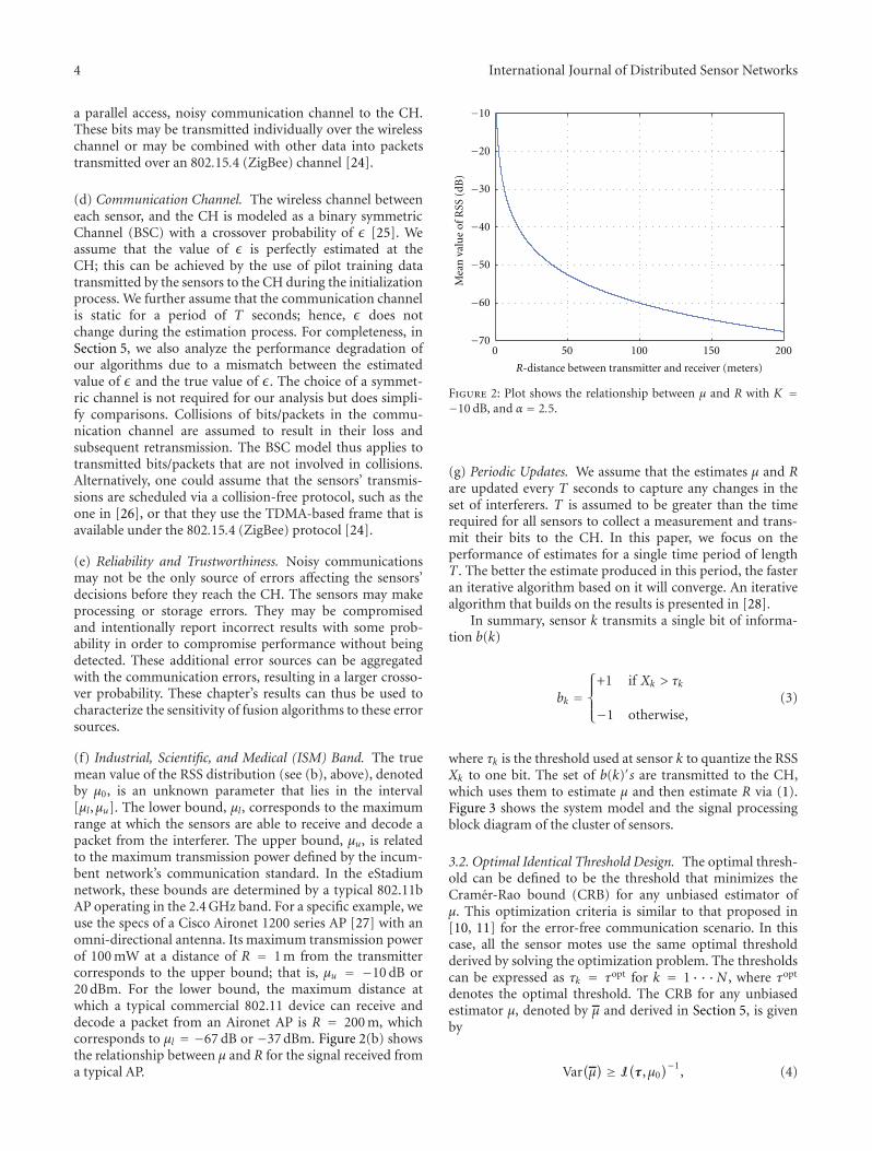
(f) Industrial, Scientific, and Medical (ISM) Band. The truemean value of the RSS distribution (see (b), above), denotedby μ0, is an unknown parameter that lies in the interval[μl,μu]. The lower bound, μl, corresponds to the maximumrange at which the sensors are able to receive and decode apacket from the interferer. The upper bound, μu, is relatedto the maximum transmission power defined by the incum-bent network’s communication standard. In the eStadiumnetwork, these bounds are determined by a typical 802.11bAP operating in the 2.4 GHz band. For a specific example, weuse the specs of a Cisco Aironet 1200 series AP [27] with anomni-directional antenna. Its maximum transmission powerof 100 mW at a distance of R = 1 m from the transmittercorresponds to the upper bound; that is, μu = −10 dB or20 dBm. For the lower bound, the maximum distance atwhich a typical commercial 802.11 device can receive anddecode a packet from an Aironet AP is R = 200 m, whichcorresponds to μl = −67 dB or −37 dBm. Figure 2(b) showsthe relationship between μ and R for the signal received froma typical AP.

0 50 100 150 200−70

−60

−50

−40

−30

−20

−10

Mea

nva

lue

ofR

SS(d

B)

R-distance between transmitter and receiver (meters)

Figure 2: Plot shows the relationship between μ and R with K =−10 dB, and α = 2.5.

(g) Periodic Updates. We assume that the estimates μ and Rare updated every T seconds to capture any changes in theset of interferers. T is assumed to be greater than the timerequired for all sensors to collect a measurement and trans-mit their bits to the CH. In this paper, we focus on theperformance of estimates for a single time period of lengthT. The better the estimate produced in this period, the fasteran iterative algorithm based on it will converge. An iterativealgorithm that builds on the results is presented in [28].

In summary, sensor k transmits a single bit of informa-tion b(k)

bk =⎧⎪⎨

⎪⎩

+1 if Xk > τk

−1 otherwise,(3)

where τk is the threshold used at sensor k to quantize the RSSXk to one bit. The set of b(k)′s are transmitted to the CH,which uses them to estimate μ and then estimate R via (1).Figure 3 shows the system model and the signal processingblock diagram of the cluster of sensors.

3.2. Optimal Identical Threshold Design. The optimal thresh-old can be defined to be the threshold that minimizes theCramer-Rao bound (CRB) for any unbiased estimator ofμ. This optimization criteria is similar to that proposed in[10, 11] for the error-free communication scenario. In thiscase, all the sensor motes use the same optimal thresholdderived by solving the optimization problem. The thresholdscan be expressed as τk = τopt for k = 1 · · ·N , where τopt

denotes the optimal threshold. The CRB for any unbiasedestimator μ, denoted by μ and derived in Section 5, is givenby

Var(μ) ≥ I

(τ,μ0

)−1, (4)


X1 = μ + n1

XN = μ + nN

b1 = +1 if X1 > τ1

bN = +1 if XN > τN

b1

bN

Sensornode 1

Sensornode N

......

... ML estimatorμ

Cluster head(fusion center)

b1 = −1 if X1 ≤ τ1

bN = −1 if XN ≤ τN

BSCε

BSCε

r1

rN

Figure 3: System block diagram for a cluster of wireless sensors. The sensor’ RSS measurements are quantized using the dithered quanti-zation technique. The resulting 1-bit values are transmitted over a BSC to the CH, which calculates the MLE of R.

where I(τ,μ0) is called the Fisher information (FI). Asderived later in the paper, the FI is expressed as

I(τ,μ0

) =N∑

k=1

I(τk,μ0

), (5)

where

I(τk,μ0

)

=((1− 2ε) fn

(τk − μ0

))2

ε + (1− 2ε)Fn(τk − μ0

)(

1− ε − (1− 2ε)Fn(τk − μ0

))

(6)

is the FI for sensor k, τ = [τ1 · · · τN ], μ0 is the true valueof μ, and Fn(·) and fn(·) are the complementary cumulativedistribution function (ccdf) and pdf of the measurementnoise n, respectively. Due to lack of space, we only outlinethe general technique to obtain the critical points of the CRBfunction. Calculating the gradient of the r.h.s of (4) withrespect to τk for k = 1 · · ·N , it can easily be shown thatwhen τk = μ0 for each k, the N equations are simultaneouslyequal to zero, and the Hessian of the CRB function is positivedefinite. Hence, the optimal threshold is τopt = μ0. Notethat this choice of threshold is not feasible because μ0 is notknown in advance.

An interesting observation is that the optimal identicalthreshold choice does not depend on σn or ε. It is onlya function of the true unknown value μ0. Furthermore,the performance of the identical threshold scheme is verysensitive to the choice of threshold, as shown in Section 6.Even a slight deviation of the threshold value from the truevalue of μ can result in significant performance degradation.Hence, our goal is to design a quantization scheme which isindependent of the true value of μ and has a performancecomparable to the optimal identical threshold case.

3.3. Threshold Design for Dithered Quantization. Because useof the optimal identical threshold for the 1-bit quantization

step requires prior knowledge of the unknown parameter, wepropose a framework in which each sensor uses a differentthreshold. This ensures that at least a few thresholds willbe close to the true value of the unknown parameter.Furthermore, using non-identical thresholds at the sensorsfor the 1-bit quantization produces a dithering effect thatreduces the bias in the estimator (as shown in Section 5). Wethus refer to this technique as dithered quantization. Since itis well known that the uniform distribution has maximumentropy among all continuous distributions with compactsupport [25], we assume that μ is uniformly distributedover the interval [μl ,μu] and hence space the quantizationthresholds equally over this interval. This leads to thethresholds being assigned for sensor mote k according to thefollowing equation:

τk = μl +k(μu − μl

)

N + 1. (7)

3.4. Binning-Based Nonidentical Threshold Design. Anotherapproach to the use of non-identical threshold was proposedin [10]. They consider designing the threshold vector τ ={τk, k ∈ Z} and the associated frequency vector ρ ={ρk, k ∈ Z} to minimize the weighted asymptotic variance.The frequency for threshold τk is defined as ρk = Nk/N ,where Nk is the total number of sensors transmitting binaryinformation using threshold τk, and N is the total numberof sensors in the network. Although the problem studied in[10] was for the error-free communication channel scenario,it can be modified for the BSC case. Hence, for our setup,this optimization problem for a uniform weighting functionbetween [μl ,μu] denoted by W(μ) = 1/(μu − μl) can beformulated as the following second-order cone program(SOCP) with auxiliary variable t as

ρ� = argmin(t,ρ)

t,

s.t.∥∥s− Pρ

∥∥ ≤ t,

ρ ≥ 0, ρT1 = 1,

(8)


where s := [S(μ0) · · · S(μM)]T , ρ := [ρ1 · · ·ρL]T , L is thenumber of thresholds, M is the number of discrete points

at which the function S(μ) is evaluated, the function S(μ) isgiven by

S(μ) =KW 1/2(μ

), K =

∫ +∞−∞

((1− 2ε) fn(u)

)2/((

ε + (1− 2ε)Fn(u))(

1− ε − (1− 2ε)Fn(u)))

du∫ +∞−∞ W 1/2

(μ)dμ

, (9)

and P is a M × L matrix with its (i, j)th entry given by

[P]i j =(

(1− 2ε) fn(

τj − μi))2

(

ε + (1− 2ε)Fn

(

τj − μi))(

1− ε − (1− 2ε)Fn

(

τj − μi)) . (10)

Using numerical techniques to approximate the numeratorof K , S(μ) can be expressed as

S(μ) =

∫ +∞−∞

((1− 2ε) fn(u)

)2/((

ε + (1− 2ε)Fn(u))(

1− ε − (1− 2ε)Fn(u)))

du∣∣μu − μl

∣∣ . (11)

For the rest of the paper, we refer to this technique asthe binning-based non-identical threshold approach. InSection 5, we compare the performance of all three thresholddesign schemes.

3.5. Effect of Network Topology on Threshold Design. Wirelesssensor networks change with time because sensors can fail astheir batteries die, or new sensors may be added to an existingnetwork. Our threshold design is robust to these changes,since when the number of sensors is large, the thresholds aredensely distributed over the interval, the loss of a few sensorswill not result in a significant loss of information. Whenthe number of sensors is small, the thresholds are coarselyspread over the interval. A few failures might thus result in asignificant decrease in the number of bits received by the CH.The CH can then reassign thresholds by communicating withthe sensors over the wireless channel. When a new sensorjoins the network, it can request a threshold from the CH,choose one based on its unique MAC address, or the CH canreassign all sensors’ thresholds according to the algorithmin Section 3.3. On the other hand, the binning-based non-identical threshold technique requires the solution to theoptimization problem (8) each time the thresholds need tobe assigned. Hence, compared to our proposed approach, thebinning-based approach is of much higher computationalcomplexity and therefore cannot easily adapt to changes inthe network topology.

4. Sensor Fusion Algorithm

We use maximum-likelihood estimation (MLE) techniquesto estimate μ and then use the invariance property of MLE’s

[29] obtain an estimate for R. For sensor mote k, we denoteRk to be the random variable (r.v) for the received bit andrk to be the value of the r.v. Since the received bits Rk areindependent, nonidentically distributed (i.n.i.d) Bernoullirandom variables (rv’s),

Pr(Rk = 1 | μ) = ε + (1− 2ε)Fn

(τk − μ

),

Pr(Rk = −1 | μ) = (1− ε)− (1− 2ε)Fn

(τk − μ

),

(12)

where Fn(·) is the complementary cumulative distributionfunction (ccdf) of the measurement noise n ∼ N (0, σ2

n).Denoting the likelihood function of each received bit byf (rk | μ), the likelihood function for the received vector ofobservations r = [r1, . . . , rN ] becomes

f(

r | μ) =N∏

k=1

f(rk | μ

)

=N∏

k=1

Pr(Rk = 1 | μ)1{rk=1}Pr

(Rk = −1 | μ)1{rk=−1} .

(13)

Let Hk(μ) = ε+(1−2ε)Fn(τk−μ), then the log-likelihoodfunction is given by

ln f(

r | μ)

=N∑

k=1

[1{rk=1} ln

(Hk(μ))

+ 1{rk=−1} ln(1−Hk

(μ))]

.

(14)


Thus, the MLE μ is obtained by solving the followingconstrained maximization problem,

argmaxμ

N∑

k=1

[1{rk=1} ln

(Hk(μ))

+ 1{rk=1} ln(1−Hk

(μ))]

,

s.t. μl ≤ μ ≤ μu,(15)

and because the function relating μ to R in (1) is one toone, the MLE R can be obtained directly from μ. Note thatwe have assumed that the CH has perfect knowledge ofthe dB spread of the log-normal shadowing, that is, σ2

n andthe cross-over probability ε. The former can usually be ob-tained offline by conducting field measurements in the areaof deployment and then performing regression analysis usingthe experimental data [30]. As for ε, this is typically knowna priori depending on the modulation and coding schemeused. For example, for transmission of information over fad-ing channels, the probability of bit error (pe) is well knownwhen standard digital modulation (BSPK, QPSF, 64-QAM,etc.) schemes are used with error control coding strategiessuch as Turbo or LDPC codes. Hence, pe can be used as thevalue for ε.

5. Performance Analysis of DitheredQuantization Approach

This section contains (i) proofs of the asymptotic consis-tency and efficiency of the MLE for μ and R using theproposed dithered quantization approach (ii) derivation ofthe Cramer-Rao bound (CRB) for the variance of any unbi-ased estimator for μ and R, and (iii) Monte Carlo simula-tions that validate the asymptotic results and compare theperformance of the dithered quantization technique with theidentical threshold-based quantization approach. Since theconstrained ML optimization in (15) is analytically intract-able, there is no closed-form expression for the estimates orthe distribution of the estimates. Hence, to study the biasof the MLE’s, we prove that the estimators are asymptoti-cally strongly consistent and hence asymptotically unbiased.Furthermore, although the R(k)’s are i.n.i.d Bernoulli r.v’s,we prove that MLE’s are asymptotically normally distributedand efficient. Monte Carlo simulations confirm these results

and, as shown later, demonstrate that these desirable asymp-totic behavior is effectively achieved with as few as 70 ∼ 100sensors.

5.1. Asymptotic Properties. For the following results, we de-fine μN , RN to be the MLE of μ and R, respectively, ob-tained with N sensors using the dithered quantization tech-nique.

Proposition 1. The MLE μN is unique and asymptoticallystrongly consistent Pr(limN→∞μN = μ0) = 1, where μ0

represents the true value of μ.

Proof. See Appendix A.

Proposition 2. μN is asymptotically efficient (μN − μ0) →D

N (0, 1/(I(μ0))), where μ0 represents the true value of μ, I(·)is the Fisher information (FI), and →

Dmeans convergence in

distribution.

Proof. See Appendix B.

The following two corollaries are immediate consequen-ces of the invariance property of functions of MLE’s and theone-to-one mapping between μ and R.

Corollary 1. The MLE RN is unique and asymptoticallystrongly consistent Pr(limN→∞RN = R0) = 1, where R0 repre-sents the true value of R.

Corollary 2. RN is asymptotically efficient (RN − R0) →D

N (0, 1/(I(R0))), where R0 represents the true value of R.

5.2. Cramer-Rao Bound. In this subsection, we derive theCRB for any unbiased estimator of μ denoted by μ. The MLEμ derived previously may be biased for small N , but sincewe have proved that it is asymptotically unbiased, the CRB isuseful as a lower bound of the variance of μ for medium-to-large numbers of sensor motes.

Theorem 1. The CRB for any unbiased estimator μ obtainedusing the dithered quantization technique with the BSC modelis

Var(μ) ≥

⎡

⎣N∑

k=1

⎧⎨

⎩

((1− 2ε) fn

(τk − μ

))2

(

ε + (1− 2ε)Fn(τk − μ

))(

1− ε − (1− 2ε)Fn(τk − μ

))

⎫⎬

⎭

⎤

⎦

−1

. (16)

Proof. See Appendix C.

Using the CRB for μ and observing that (1) is a one-to-one transformation, the CRB for any unbiased estimatorof R, denoted by R, can be derived using the invarianceproperty of MLE’s and functions of MLE’s. The followinglemma relates the variance of μ to the variance of R.

Lemma 1. If R = g(μ), then the variance of any unbiasedestimate of R is given by

Var(

R)

≥(∂g/∂μ

)2

I(μ0) . (17)


Proof. A proof of this lemma can be found in [29, Chapter3, Appendix 3A].

Corollary 3. The CRB for any unbiased estimator for R usingthe dithered quantization technique with the BSC model is

Var(

R)

≥(

(ln 10)10(K−μ)/10α/10α)2

I(μ) , (18)

where

I(μ)

=N∑

k=1

⎧⎨

⎩

((1−2ε) fn

(τk−μ

))2k(

ε+(1−2ε)Fn(τk−μ

))(

1−ε−(1−2ε)Fn(τk−μ

))

⎫⎬

⎭

(19)

is the FI.

Proof. Using Lemma 1 and the relationship between R and μgiven by R = 10(K−μ)/10α, the result follows.

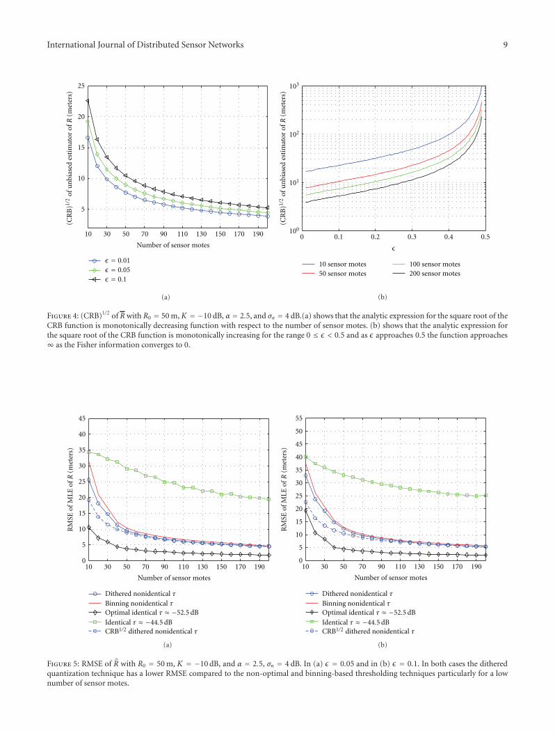
Figures 4(a) and 4(b) show the behavior of the squareroot of the CRB of R when we vary the number of sensors,N , and the crossover probability, ε, respectively. The CRB isa monotonically increasing function of ε for 0 ≤ ε < 0.5and, due to its symmetry about ε = 0.5, is a monotonicallydecreasing function for 0.5 < ε ≤ 1. As ε → 0.5 theCRB tends to ∞ because, from (1), the Fisher informationconverges to 0. From Figure 4(a), we observe that the CRB isa monotonically decreasing function of N , which is expectedbecause more sensors means more observations, thus, lowerCRB values. Although MLE’s tend to have a significant biasfor small sample sizes, we have proved that the MLE for ourscheme is asymptotically strongly consistent and efficient.Therefore, the analytic derivations above for the CRB forμ and R hold in the asymptotic region. The simulationresults in the following subsection show that the asymptoticbehavior is achieved even with a small number of sensors.

5.3. Numerical Simulation Results. To evaluate the perfor-mance of the dithered quantization scheme and compareit with the identical and the binning-based non-identicalthreshold approaches, we now conduct numerical MonteCarlo simulations. In these simulations (i) the number ofsensors is varied from 10 to 200 and (ii) both a low ε of0.05 and a high ε of 0.1 are considered. The value of R0 isset to 50 m, which corresponds to μ0 ≈ −52.5 dB and Kis set to −10 dB, the maximum transmission power allowedfor 802.11b. We use the typical value of 2.5 for the path-lossexponent α. The standard deviation of the RSS distributionobserved at the sensor motes is set to 4 dB; that is, σn = 4 dB.

The results obtained were averaged over 2000 realizationsof the measurement noise process. It can easily be shown(see Appendix D) that the log-likelihood function is nota concave function of μ for both non-identical threshold-based approaches. Hence, we implemented an 1-dimensionaliterated grid search algorithm [31] to locate an approximate

maximal value of the log-likelihood function denoted by L.We employed an equidistance grid of size n points given as:

S ={

xk | xk = μl +k(μu − μl

)

n− 1, k = 0 · · ·n− 1

}

. (20)

Using the grid S, the values L(x1), L(x2) · · ·L(xn) are usedin the grid search algorithm. An approximate local maximumis located by choosing the grid point xk that has the largestvalue for L(xk). Using this initialization point, we then usedMatlab’s sequential quadratic programming (SQP) methodto perform the local optimization to determine the MLE.

To characterize the computational complexity of theoptimization algorithm, we note that the local optimizationusing SQP has quadratic convergence rate. The computa-tional complexity of the iterative grid search algorithm canbe expressed as C(n, r) = rnm, where m is the dimension ofthe parameter space, n is the grid size, and r is the numberof iterations. In our simulation experiments, we found thatwith r = 10 and a grid size of n = 100 the algorithmconverged to an approximate local maximal point quickly.Hence, the computational complexity of the grid search forour case is O(n). In our Matlab implementation of the gridsearch algorithm, we were able to reduce the complexity toO(n log n), by the use of sorting algorithms to find the gridpoint xk that would correspond to the largest value of the log-likelihood function L(xk). In a practical setting, the searchgrid will be precomputed, and the algorithm will be executedon the CH. Since the CH typically has more processing powerthan other motes, in a practical setting the convergence of thealgorithm would be very fast.

The non-identical thresholds for the dithered quantiza-tion technique are generated using the technique describedin Section 3, and, for the binning-based technique the SOCP7 is solved in Matlab using cvx software [32]. As mentionedin [10], the threshold spacing for the binning technique isset to 2σn, and hence we have τk+1 − τk = 8 dB, thereforethe number of threshold bins B = (μu − μl)/8 = 8.For the case where an identical threshold is used by allsensor motes, we consider two scenarios. In the first case,the optimal threshold is used; that is, τ = μ0, whichcorresponds to τ ≈ −52.5 dB. In the second case, an identicalnonoptimal threshold is used, this corresponds to choosing τabove/below the true mean value of the RSS distribution; thatis, τ = (μ0 + Δ) dB. For simulation purposes, we set Δ = 8;this corresponds to τ ≈ −44.5 dB. Similar simulation resultsare obtained for the case when τ > τopt.

In Figures 5(a) and 5(b), we plot the root mean squarederror (RMSE) of R for the low and high ε cases. We observethat the RMSE using the dithered quantization approach islower for a small number of sensor motes compared to thenon-optimal identical threshold approach and the binning-based non-identical approaches. As the number of sensormotes is increased the RMSE of the binning-based non-identical technique converges to the dithered quantizationtechnique. This is expected since for the binning basedapproach as the number of sensor motes is increasedthe threshold frequency (ρk) increases which leads to theimprovements in the performance.


10 30 50 70 90 110 130 150 170 190

5

10

15

20

25

Number of sensor motes

(CR

B)1/

2of

un

bias

edes

tim

ator

ofR

(met

ers)

ε = 0.01ε = 0.05ε = 0.1

(a)

0 0.1 0.2 0.3 0.4 0.5100

101

102

103

(CR

B)1/

2of

un

bias

edes

tim

ator

ofR

(met

ers)

10 sensor motes50 sensor motes

100 sensor motes200 sensor motes

ε

(b)

Figure 4: (CRB)1/2 of R with R0 = 50 m, K = −10 dB, α = 2.5, and σn = 4 dB.(a) shows that the analytic expression for the square root of theCRB function is monotonically decreasing function with respect to the number of sensor motes. (b) shows that the analytic expression forthe square root of the CRB function is monotonically increasing for the range 0 ≤ ε < 0.5 and as ε approaches 0.5 the function approaches∞ as the Fisher information converges to 0.

10 30 50 70 90 110 130 150 170 1900

5

10

15

20

25

30

35

40

45


RM

SEof

MLE

ofR

(met

ers)

Dithered nonidentical τBinning nonidentical τOptimal identical τ ≈ −52.5 dB

Identical τ ≈ −44.5 dBCRB1/2 dithered nonidentical τ

(a)

10 30 50 70 90 110 130 150 170 1900

5

10

15

20

25

30

35

40

45


RM

SEof

MLE

ofR

(met

ers)

50

55

Dithered nonidentical τBinning nonidentical τOptimal identical τ ≈ −52.5 dB

Identical τ ≈ −44.5 dBCRB1/2 dithered nonidentical τ

(b)

Figure 5: RMSE of R with R0 = 50 m, K = −10 dB, and α = 2.5, σn = 4 dB. In (a) ε = 0.05 and in (b) ε = 0.1. In both cases the ditheredquantization technique has a lower RMSE compared to the non-optimal and binning-based thresholding techniques particularly for a lownumber of sensor motes.


10 30 50 70 90 110 130 150 170 1900

2

4

6

8

10

12

14

16

18

20


Bia

sof

MLE

ofR

(met

ers)

Dithered nonidentical τBinning nonidentical τOptimal identical τ ≈ −52.5 dBIdentical τ ≈ −44.5 dB

(a)

10 30 50 70 90 110 130 150 170 190


0

5

10

15

20

25

30

Bia

sof

MLE

ofR

(met

ers)

Dithered nonidentical τBinning nonidentical τOptimal identical τ ≈ −52.5 dBIdentical τ ≈ −44.5 dB

(b)

Figure 6: Bias of R with R0 = 50 m, K = −10 dB, and α = 2.5, σn = 4 dB. In (a) ε = 0.05 and in (b) ε = 0.1. In both cases the dith-ered quantization technique has a lower bias compared to the non-optimal and binning-based thresholding techniques especially for a lownumber of sensor motes.

Figures 6(a) and 6(b) show the bias of R versus the num-ber of sensor motes. We notice that the bias of the MLE us-ing the dithered quantization technique is lower than thenon-optimal estimators. Furthermore, we also observe thatthe bias decreases at an exponential rate with respect to thenumber of sensor motes and approaches close to 0 withabout 100 sensor motes. Figures 5 and 6 also show that theasymptotic properties of the MLE are achievable with about50 sensor motes for low values of ε and about 70 sensormotes for high values of ε.

In Figures 7(a) and 7(b), we compare the performanceloss incurred using the different thresholding techniques.We define the CRBLoss = CRBnon-opt − CRBopt, whereCRBnon−opt is the CRB of any unbiased estimator using eitherthe dithered quantization, binning-based or identical non-optimal thresholding techniques, and CRBopt is the CRB ofany unbiased estimator using the optimal identical threshold.This metric serves as a good benchmark as, for large numberof sensor motes, the MLE’s are unbiased, and hence the MSEis equal to the CRB. Figures 7(a) and 7(b) show the CRBLoss

versus the number of sensors. We observe that for low andhigh ε values the loss is significantly less for the ditheredquantization technique compared with the other schemes,particularly for a small number of sensor motes which is im-portant from a practical point of view.

Figure 8 shows the robustness of our scheme due to amismatch in the true value of ε and the value of ε usedby the CH for the ML estimation. We notice that even ifthere is a mismatch, the performance degradation is not sig-nificant. The performance of having a perfectly estimatedvalue of ε can be replicated using more sensor motes under

the condition of a mismatch in ε. Furthermore, the gap be-tween the performance between the perfectly estimated ε andthe mismatched ε decreases as the number of sensor motesincreases.

In a realistic situation in which the mean of the RSS dis-tribution at the sensor nodes is unknown priori, there is noway to choose the optimal τ for the identical threshold case. Itwill thus be difficult to achieve good/reliable estimates usingnon-optimal identical thresholds. In this type of practicalscenario, if both approaches (non-optimal identical and non-identical thresholds) use the same number of sensors, andeach sensor samples the RSS once, then using the non-iden-tical threshold approach would produce a much more accu-rate estimate.

Although both non-identical thresholding approachesrequire fewer sensors than the non-optimal identical thresh-old technique to achieve near-optimal performance, weobserve that compared to the binning approach our thresh-olding scheme is of low complexity, as it does not involvesolving any complex optimization problem to design thethresholds. Furthermore, the dithered quantization tech-nique performs better in terms of having a lower RMSE,variance, and bias compared with the binning and non-opti-mal identical thresholding techniques, particularly when thenumber of sensors is small, which is the typical case in a prac-tical scenario.

In summary, the dithered quantization technique has sig-nificant advantages over other techniques in terms of eitherthe number of sensors required to achieve a given accuracyor the accuracy of estimates achievable with a fixed numberof sensors.


10 30 50 70 90 110 130 150 170 1900

100

200

300

400

500

600

700

800

900


CR

Blo

ss

Dithered nonidentical τBinning nonidentical τIdentical τ ≈ −44.5 dB

(a)

10 30 50 70 90 110 130 150 170 190


0

200

400

600

800

1000

1200

1400

1600

1800

2000

CR

Blo

ss

Dithered nonidentical τBinning nonidentical τIdentical τ ≈ −44.5 dB

(b)

Figure 7: (CRB)1/2 with R0 = 50 m, K = −10 dB, α = 2.5, and σn = 4 dB. In (a) ε = 0.05 and in (b) ε = 0.1, in both cases the loss incurredusing the dithered quantization technique is significantly less compared to the other techniques, particularly for low number of sensor motes.

10 30 50 70 90 110 130 150 170 1900

5

10

15

20

25

30

35


RM

SEof

MLE

ofR

(met

ers)

ε = 0ε = 0.05ε = 0.1

Figure 8: shows the RMSE of R using dithered quantization technique with R0 = 50 m, K = −10 dB, α = 2.5, and σn = 4 dB for variousvalues of ε. The plot shows the robustness of our estimation scheme due to a mismatch in the true value of ε and the estimated value of εused by the CH.

6. Drawbacks of the IdenticalThreshold Approach

In this section, we study the disadvantages of using theidentical threshold approach and the effect on R using this

technique. As observed in previous work [10, 11], with theerror-free communication channel, the disadvantage of theidentical threshold approach is that the CRB for μ growsexponentially with [(τ−μ0)2/σn]2. A similar observation canbe seen for the CRB of R when the identical threshold is


used under a BSC model. Using the tight Chernoff boundfor the ccdf of the Gaussian distribution (i.e., Fn(τ − μ) ≤e−(τ−μ)2/2/2), the CRB for R can be bounded as follows:

CRB(ε, τ,R0)

= G

[

ε+(1−2ε)Fn(τ−μ0

)][

(1−ε)−(1−2ε)Fn(τ−μ0

)]

N[(1−2ε) fn

(τ−μ0

)]2

≤ Gπσ2

ne(τ−μ0)2/2σ2

n

2N(1−2ε)2

×[(

2ε+(1−2ε)e−(τ−μ0)2/2σ2n

)

×(

2(1−ε)−(1−2ε)e−(τ−μ0)2/2σ2n

)]

,

(21)

where G = ((ln 10)10(K−μ0)/10α/10α)2. Figure 9(a) shows theexponential increase with respect to (τ − μ0)/σn for ε = 0.01and ε = 0.1 for the CRB of R. We notice that the Chernoffbound is tight and that a small deviation of τ from thetrue unknown value μ0 will result in a significant loss inperformance. Although a similar result has previously beenwidely reported for the error-free channel case [10, 11], to thebest of our knowledge, no one has studied the performanceof the MLE’s in terms of the MSE and variance effects usingthe identical threshold approach. Hence, to further analyzethe effects of using this technique, Figure 9(b) shows theMSE and variance plot as (τ − μ0)/σn is varied. As withthe CRB plot, the performance degradation in terms of theMSE is also exponential as τ deviates from μ0. However, wenotice the existence of multiple critical points. This effectis because the MSE can be decomposed into the (bias)2

and variance. The figure shows that for small deviationsfrom μ0 the (bias)2 is nearly zero, and the variance increasesexponentially; however, when τ μ0, the variance startsto decrease, but the bias increases linearly with (τ − μ0).These combined effects reiterate the fact that using identicalthresholds could potentially result in estimators with veryhigh bias and MSE.

7. Conclusion

In this paper, we proposed and analyzed a sensor fusionalgorithm for interference characterization in wireless net-works. To minimize energy usage, each wireless sensor in thenetwork transmits only 1-bit of quantized, noisy RSS infor-mation to the FC over a BSC.

Unlike previous approaches that used identical thresh-olds for all sensors or use non-identical thresholds basedon solving a complex optimization problem, we proposea simple and low complexity threshold design techniqueof uniformly distributing the thresholds over the range ofpossible values of the mean of the RSS distribution. This ap-proach performs (i) as well as the optimal identical thresholdapproach and (ii) significantly better than the identical non-optimal threshold design approaches and has a performancethat is more accurate or as good as previously proposed non-

identical threshold techniques. The optimal identical thresh-old case is highly unrealistic because the optimal thresholdcannot be known in advance; our non-identical thresholdtechnique is much more practical, reliable, and of low com-plexity design compared to previously proposed techniquesbased on either using non-identical or identical non-optimalthresholds.

Appendices

A. Asymptotic Consistency of MLE

Proof. We start with the following assumptions that are re-stated from [33, page 443-444] for completeness and are easyto verify the following.

(A0) The distributions F(R | μ) of the observations aredistinct.

(A1) The distributions F(R | μ) have common support.

(A2) The observations are r = (r1, . . . , rN ), where the rk areindependent with probability density f (rk | μ) withrespect to the underlying probability measure.

(A3) The parameter space Ω contains an open set ω ofwhich the true parameter value μ0 is an interior point.

Next, we prove the following lemma.

Lemma 2. For the independent nonidentically distributed(i.n.i.d) random variables Rk’s we have

Pr{

limN→∞

ln f(

R | μ)

< ln f(

R | μ0

)}

= 1, ∀μ /= μ0,

(A.1)

where μ0 is the true value of μ.

Proof. To prove the lemma, it is equivalent to prove thefollowing:

Pr

⎧⎨

⎩limN→∞

⎡

⎣1N

N∑

k=1

lnf(Rk | μ

)

f(Rk | μ0

) < 0

⎤

⎦

⎫⎬

⎭= 1, ∀μ /= μ0.

(A.2)

Next, we show that the strong law of large numbers (SLLNs)can be applied to the term (1/N)

∑Nk=1 ln f (Rk | μ)/ f (Rk |

μ0). To show this, we check the Kolmogorov sufficientconditions for the SLLN to hold for independent r.v.’s. LetYk = ln f (Rk | μ)/( f (Rkμ0)), pk = Pr(Rk = 1 | μ),qk = Pr(Rk = −1 | μ) = (1 − pk), pk0 = Pr(Rk = 1 | μ0)and qk0 = Pr(Rk = −1 | μ0). We further assume w.l.o.g. thatε ≤ 0.5, and using (12) we have the following inequalities:

ε ≤ pk ≤ 1− ε,

1− ε ≤ qk ≤ ε.(A.3)


−4 −3 −2 −1 0 1 2 3 4100

101

102

103

104

105

106

(τ − μ0)/σn

CR

Bfo

ru

nbi

ased

esti

mat

orof

R(m

eter

s2)

CRB ε = 0.01Chernoff bound ε = 0.01CRB ε = 0.1Chernoff bound ε = 0.1

(a)

−4 −2 0 2 4 6

200

400

600

800

1000

1200

1400

1600

(τ − μ0)/σn

MSE

vari

ance

and

bias

2of

MLE

ofR

(met

ers2

)

MSE ε = 0.01Variance ε = 0.01Bias2 ε = 0.01

MSE ε = 0.1Variance ε = 0.1

Bias2 ε = 0.1

(b)

Figure 9: In (a) the CRB and the Chernoff bound for R is shown for varyious values of τ at R0 = 50 m (μ0 ≈ −52.5 dB), N = 100 andσn = 4 dB. Observe that the performance degradation is exponential as (τ − μ0)/σn increases for different crossover probabilities. (b) showsthe MSE, variance and (bias)2 for R with varying τ with R0 = 50 m (μ0 ≈ −52.5 dB) N = 100 and σn = 4 dB. The MSE also has an exponentialgrowth with respect to (τ − μ0)/σn; however, we notice the peculiar behavior of multiple critical points due to the bias and variance effect ofthe MLE of R.

Similar inequalities hold for pk0 and qk0 , respectively. Thevariance of Yk can be bounded as follows:

Var(Yk) ≤ Eμ0

[

Yk2]

= pk0

(

lnpkpk0

)2

+ qk0

(

lnqkqk0

)2

≤ (1− ε)(

ln(1− ε)ε

)2

+ ε(

lnε

(1− ε)

)2

= 1.

(A.4)

Therefore, limN→∞∑N

k=1 Var(Yk)/k2 ≤ limN→∞∑N

k=1(1/k2)<∞, hence, the SLLN holds for Yk’s, and we have

Pr

⎧⎨

⎩limN→∞

1N

⎡

⎣N∑

k=1

lnf(Rk | μ

)

f(Rk | μ0

)

−N∑

k=1

Eμ0

(

lnf(Rk | μ

)

f(Rk | μ0

)

)

= 0

⎤

⎦

⎫⎬

⎭= 1,

(A.5)

where Eμ0 (·) represents the expectation using the pdf whenμ = μ0. Now by Jensen’s inequality we have

Eμ0

[

lnf(Rk | μ

)

f(Rk | μ0

)

]

< lnEμ0

⎡

⎣f(Rk | μ

)

f(

Rk| μ0

)

⎤

⎦

= ln

[Pr(R1 = 1 | μ)

Pr(R1 = 1 | μ0

)Pr(R1 = 1 | μ0

)

+Pr(R1 = −1 | μ)

Pr(R1 = −1 | μ0

)Pr(R1 = −1 | μ0

)]

= ln[Pr(R1 = 1 | μ) + Pr

(R1 = −1 | μ)]

= 0.

(A.6)

Using the result (A.6) in (A.5), statement (A.2) is proved, andhence the lemma follows.

Next we consider a δ-neighborhood about μ0 such that(μ0 − δ,μ0 + δ) ∈ ω and define SN = {r : ln f (r | μ0 − δ) <ln f (r | μ0) and ln f (r | μ0) > ln f (r | μ0 + δ)}. Hence, byLemma 2 we have,

Pr{

limN→∞

SN | μ0

}

= 1 (A.7)


and, therefore, for all r ∈ SN , there exists μN ∈ (μ0 − δ,μ0 +δ) s.t. the likelihood function is maximized in the interval.Since for any δ > 0 small enough, there exists a sequenceμN = μN (δ) of roots to the equation ∂ ln f (r | μ)/∂μ = 0s.t. Pr{limN→∞ | μN − μ0 |< δ | μ0} = 1. Next we choose asequence which does not depend on δ, by observing that thelikelihood function is a continuous function, and the limitof a sequence of roots is also another root of the equation∂ ln f (r | μ)/∂μ = 0. Therefore, there exists a root μ∗N that isclosest to μ0; hence, Pr(limN→∞ | μ∗N − μ0 |< δ | μ0) = 1 andsince δ was arbitrary chosen the proposition follows.

B. Asymptotic Efficiency of MLE

Proof. The key step is to show that the central limit theorem(CLT) holds for the i.n.i.d log-likelihood functions of theRk’s. As before, we state the following regularity conditionsfrom [33, page 440-441] for completeness.

(a) The parameter space Ω is an open interval (notnecessarily finite).

(b) The distributions of F(Rk | μ) have commonsupport, so that the set A = {rk : f (rk | μ) > 0} isindependent of μ.

(c) For every rk ∈ A, the density f (rk | μ) is twicedifferentiable with respect to μ, and the second deriv-ative is continuous in μ

(d) E[∂ ln f (Rk | μ)/∂μ] = 0 and E[−∂2 ln f (Rk |μ)/∂μ2] = E[(∂ ln f (Rk | μ)/∂μ)2] = I(μ).

(e) The Fisher information 0 < I(μ) < ∞.

(f) For any given μ0 ∈ Ω, there exists a positive numberc and a function M(rk) (both of which may dependon μ0) s.t.

∣∣∣∣∣

∂2 ln f(rk | μ

)

∂μ2

∣∣∣∣∣≤M(rk), ∀rk ∈ A, μ0 − c < μ < μ0 + c,

(B.1)

and Eμ0 [M(Rk)] <∞.Since most of the conditions listed above are easy to

verify, we provide proofs only for (d) and (f). To provethe first part of (d) we need to show that Eμ0 [∂ ln f (Rk |μ)/∂μ] = 0. Using the definitions for pk and qk fromAppendix A, we have p′k = (1 − 2ε) fn(τk − μ), q′k = −(1 −2ε) fn(τk−μ), p′′k = (1−2ε) fn(τk−μ)/σ2

n , and q′′k = p′′k , where

the notation f ′ = ∂ f /∂μ and f ′′ = ∂2 f /∂μ2. Therefore, using

(12), we have

Eμ0

[∂ ln f

(R | μ)∂μ

]

= pk0

(p′kpk

)

+ qk0

(q′kqk

)

= pk0

(p′kpk

)

+(1− pk0

)(

p′k(1− pk

)

)

= 0.(B.2)

Similarly we have

Eμ0

⎡

⎣

(∂ ln f

(R | μ)∂μ

)2⎤

⎦ = pk0 p′k

2

pk2+qk0q

′k

2

qk2,

E

[−∂2 ln f(Rk | μ

)

∂μ2

]

= −⎛

⎝pk0

(

p′′k pk − p′k2)

pk2

+qk0

(

q′′k qk − q′k2)

qk2

⎞

⎠

= − pk0 p′′k

pk+qk0 p

′′k

qk

+pk0 p

′k

2

pk2+qk0q

′k

2

qk2

= pk0 p′k

2

pk2+qk0q

′k

2

qk2.

(B.3)

To check condition (f) using the result from Appendix D wehave for all rk ∈ A, μ0 − c < μ < μ0 + c∣∣∣∣∣

∂2 ln f(rk | μ

)

∂μ2

∣∣∣∣∣≤ 1{rk=1}

((μu − μl

)(1− 2ε)√

2πσ3n

)

+ 1{rk=−1}

((μu − μl

)(1− 2ε)√

2πσ3n

)

.

(B.4)

If we let M(rk) = 1{rk=1}((μu − μl)(1 − 2ε)/√

2πσ3n) +

1{rk=−1}((μu − μl)(1− 2ε)/√

2πσ3n), and hence

Eμ0 [M(Rk)] = pk0

((μu − μl

)(1− 2ε)√

2πσ3n

)

+ qk0

((μu − μl

)(1− 2ε)√

2πσ3n

)

< ∞.

(B.5)

Next we prove the CLT for independent nonidenticallydistributed (i.n.i.d) r.v.’s, which will be used to show theasymptotic efficiency result.

Lemma 3. For the independent, nonidentically distributed(i.n.i.d) log-likelihood function ln f (R | μ0), we have

1√N

∂

∂μ0ln f

(

R | μ0

)

→D

N

(

0,I(μ0)

N

)

, (B.6)

where μ0 is the true value of μ, I(μ0) =∑Nk=1(1− 2ε)2 f 2

n (τk −μ0)/pk0qk0 is the Fisher information matrix, pk0 = Pr(Rk =1 | μ0), qk0 = Pr(Rk = −1μ0), and →

Dmeans convergence in

distribution.

Proof. For ease of notation let Yk = ∂/∂μ0 ln f (Rk | μ0),σ2Yk= Eμ0 [Y 2

k ], due to the regularity conditions, we haveEμ0 [Yk] = 0. Therefore, the l.h.s of (B.6) can be written as

1√N

∂

∂μ0ln f

(

R | μ0

)

=√N

N

N∑

k=1

Yk. (B.7)


Since the Yk’s are not i.i.d., to apply the CLT we must verifythe Lindeberg sufficiency condition. Hence we need to showthat for all ε > 0,

L(N) = 1S2N

N∑

k=1

Eμ0

{

|Yk|2}

1{|Yk|>εSN } →N→∞

0, (B.8)

where S2N = ∑N

k=1 σ2Yk

. It can be shown that σ2Yk= (1 −

2ε)2 f 2n (τk − μ0)/pk0qk0 , where pk0 = Pr(Rk = 1 | μ0) and

qk0 = Pr(Rk = −1 | μ0). Using this we have

S2N =

N∑

k=1

(1− 2ε) f 2n

(τk − μ0

)

pk0qk0

(a)≥ 4(1− 2ε)

N∑

k=1

f 2n

(τk − μ0

),

(B.9)

where (a) in (B.9) follows from the fact that 1/pk0qk0 ≥ 4 forpk0 , qk0 ∈ (0, 1). Therefore,

L(N) = 1S2N

N∑

k=1

∫

{|Yk|>εSN }|Yk|2dF(Yk)

= 1S2N

N∑

k=1

∫

R|Yk|21{|Yk|>εSN }dF(Yk).

(B.10)

We observe that from (B.9) that S2N →

N→∞∞ hence

limN→∞

L(N) = limN→∞

1S2N

N∑

k=1

∫

R|Yk|21{|Yk|>εSN }dF(Yk) = 0,

(B.11)

where (B.11) follows from the fact that limN→∞∫

R |Yk|21{|Yk|>εSN }dF(Yk) = 0 by the Lebesgue dominated

convergence theorem. Hence, the Lindeberg conditions aresatisfied and the result follows.

For rest of the proof, let L′(μ) = ∑Nk=1(∂/∂μ) ln f (Rk |

μ), L′′(μ) = ∑Nk=1(∂2/∂μ2) ln f (Rk | μ). Then, by the mean

value theorem, ∃ λ ∈ (0, 1) with μ∗N = μ0 + λ(μN − μ0) forsome μ∗N ∈ (μ0, μN ) such that L′′(μN ):

L′(μN) = L′(μ0

)+(μN − μ0

)L′′(μ∗N

). (B.12)

Since μN is the MLE, the l.h.s. of (B.12) is equal to 0. We thusobtain

√N(μN − μ0

) =(1/√N)L′(μ0

)

−(1/N)L′′(μ∗N) . (B.13)

Now since μN is a strongly consistent estimator of μ0, wehave μ∗N →

Pμ0, where →

Pmeans convergence in probability.

This implies −(1/N)L′′(μ∗N ) →P

−(1/N)L′′(μ0), by the

fact that if μ∗N →P

μ0, then g(μ∗N) →P

g(μ0) for a con-

tinuous function g(·). Using arguments similar to those inAppendix A, it can be shown that the Kolmogorov sufficientconditions for the SLLN are satisfied for (1/N)L′′(μ0), hence−(1/N)L′′(μ0) →

PI(μ0)/N . By the CLT proved earlier, we

have (1/√N)L′(μ0) →

DN (0, I(μ0)/N). Hence by Slutsky’s

theorem, we thus have√N(μN − μ0) →

DN (0,N/I(μ0)) and

the proposition follows.

C. Cramer-Rao Bound

Proof. Using the definition of Fisher information matrix, wehave

−Eμ⎡

⎣∂2 ln f

(

R | μ)

∂μ2

⎤

⎦ = −N∑

k=1

Eμ0

[∂2 ln f

(Rk | μ

)

∂μ2

]

= −N∑

k=1

[∂2 ln f

(Rk = 1 | μ)∂μ2

Pr(Rk = 1 | μ)

+∂2 ln f

(Rk = −1 | μ)∂μ2

Pr(Rk = −1 | μ)

]

.

(C.1)

Differentiating ln f (Rk = 1 | μ) and ln f (Rk = −1 | μ) withrespect to μ twice, we have:

∂2 In f(Rk = 1 | μ)∂μ2

= −(1− 2ε)2 f 2n

(τk − μ

)+ Pr

(Rk = 1 | μ)(1− 2ε) f ′n

(τk − μ

)

P(Rk = 1 | μ)2 ,

∂2 In f(Rk = −1 | μ)∂μ2

= −(1− 2ε)2 f ′n(τk − μ

)Pr(Rk = −1 | μ)− (1− 2ε)2 fn

2(τk − μ)

Pr(Rk = −1 | μ)2 .

(C.2)


Using (C.2) and (C.1) can be expressed as

I(μ0) = −

N∑

k=1

⎧⎨

⎩

((1− 2ε) fn

(τk − μ

))2

(

ε + (1− 2ε)Fn(τk − μ

))(

1− ε − (1− 2ε)Fn(τk − μ

))

⎫⎬

⎭. (C.3)

Hence Theorem 1 is proved.

D. Concavity of Log-Likelihood Function

Lemma 4. The log-likelihood function ln f (r | μ) is not aconcave function.

Proof. Let G(μ) = ∑Nk=1(1{rk=1} lnαk(μ) + 1{rk=−1} lnβk(μ)),

where α(μ) = ε + (1− 2ε)Fn(τk − μ), β(μ) = (1− ε) − (1−2ε)Fn(τk − μ), and w.l.o.g we assume that ε < 0.5. From theproperties of concave functions, we know that if α(μ) andβ(μ) are concave and positive, thenG(μ) is concave. Considerthe terms αk(μ) and βk(μ), the first and second derivatives ofthese terms can be expressed as

α′k(μ) = (1− 2ε) fn

(τk − μ

),

α′′k(μ) =

(τk − μ

)α′k(μ)

σ2n

,

β′k(μ) = −(1− 2ε) fn

(τk − μ

) = −α′k(μ),

β′′k(μ) = −(τk − μ

)α′k(μ)

σ2n

.

(D.1)

Using the above equations, we can express the secondderivative of the log-likelihood function as

G′′(μ) =

N∑

k=1

(

1{rk=1}[

Ak(μ)(τk − μ

)− (Bk(μ))2]

+1{rk=−1}[

−Ck(μ)(τk − μ

)− (Dk(μ))2])

,

(D.2)

where Ak(μ) = α′k(μ)/σ2nαk(μ), Bk(μ) = α′k(μ)/αk(μ),

Ck(μ) = α′k(μ)/σ2nβk(μ), and Dk(μ) = α′k(μ)/βk(μ). For

G(μ) to be concave, a sufficient condition is that for all μ ∈[μl,μu],G′′(μ) ≤ 0, it can be seen from (D.2) that dependingon the values of τk and the received bits rk the sufficiencycondition may not be satisfied. For example, consider thescenario with N = 2 in this case τ1 ≈ −29.2 dB, andτ2 ≈ −48.4 dB. With the received vector r = [r1r2] = [1 1],the second derivative of the log-likelihood function can beexpressed as

G′′(μ) = α′1

(μ)(τ1 − μ

)

σ2nα1

(μ) −

(α′1(μ)

α1(μ)

)2

+α′2(μ)(τ2 − μ

)

σ2n

(1− α2

(μ)) −

(α′2(μ)

(1− α2

(μ))

)2

.

(D.3)

An equivalent sufficiency condition to show that G(μ) isconcave is if −G′′(μ) ≥ 0, for all μ ∈ [μl ,μu]. Using thedefinitions of αk(μ) and α′k(μ), we can obtain the followingupper bounds

α′k(μ) ≤ (1− 2ε) fn(0) = (1− 2ε)√

2πσn,

1(1− ε)

≤ 1αk(μ) ≤ 1

ε.

(D.4)

Then −G′′(μ) can be upper bounded as follows:

−G′′(μ) = α′1(μ)(μ− τ1

)

σ2nα1

(μ) +

(α′1(μ)

α1(μ)

)2

+α′2(μ)(μ− τ2

)

σ2n

(1− α2

(μ))

+

(α′2(μ)

(1− α2

(μ))

)

≤ (1− 2ε)(μ− τ1

)

ε√

2πσ3n

+(

1− 2ε√2πσnε

)2

+(1− 2ε)

(μ− τ2

)

ε√

2πσ3n

+(

1− 2ε√2πσnε

)2

= (1− 2ε)εσ2

n√π

(2μ− (τ1 + τ2)√

2σn+

(1− 2ε)ε√π

)

≈ (1− 2ε)εσ2

n√π

(2μ + 77.6√

2σn+

(1− 2ε)ε√π

)

.

(D.5)

It can be seen from (D.5) that for μl ≤ μ ≤ √2σn(2ε −

1)/(2ε√π)− 38.8 the second derivative of the log-likelihood

function−G′′ < 0 and henceG(μ) will not be concave for thisrange of μ. With ε = 0.1, we have that for μl ≤ μ < −51.6 dBG′′(μ) > 0. Therefore, we can conclude that log-likelihoodfunction is not concave for all μ ∈ [μl ,μu].

References

[1] X. Zhong, H. H. Chan, T. J. Rogers, C. P. Rosenberg, and E. J.Coyle, “The development and eStadium testbeds for researchand development of wireless services for large-scale sportsvenues,” in Proceedings of the 2nd International IEEE/Create-Net Conference on Testbeds and Research Infrastructures for theDevelopment of Networks and Communities (TRIDENTCOM’06), pp. 340–348, March 2006.

[2] A. Ault, J. V. Krogmeier, S. R. Dunlop, and E. J. Coyle,“eStadium: the mobile wireless football experience,” in Pro-ceedings of the 3rd International Conference on Internet and WebApplications and Services (ICIW ’08), pp. 644–649, June 2008.


[3] X. Zhong and E. J. Coyle, “eStadium: a wireless “living lab” forsafety and infotainment applications,” in Proceedings of the 1stInternational Conference on Communications and Networkingin China (ChinaCom ’06), 2007.

[4] A. Hills, “Smart Wi-Fi,” Scientific American, vol. 285, no. 10,pp. 86–94, 2005.

[5] J. K. Nelson and M. R. Gupta, “An EM technique for multipletransmitter localization,” in Proceedings of the 41st AnnualConference on Information Sciences and Systems (CISS ’07), pp.610–615, March 2007.

[6] J. K. Nelson, M. U. Hazen, and M. R. Gupta, “Global optimiza-tion for multiple transmitter localization,” in Proceedings of theMilitary Communications Conference (MILCOM ’06), pp. 1–7,October 2006.

[7] T. Roos, P. Myllymaki, and H. Tirri, “A statistical modelingapproach to location estimation,” IEEE Transactions on MobileComputing, vol. 1, no. 1, pp. 59–69, 2002.

[8] X. Liu and S. Shankar, “Sensing-based opportunistic channelaccess,” Mobile Networks and Applications, vol. 11, no. 4, pp.577–591, 2006.

[9] K. R. Chowdhury and I. F. Akyildiz, “Cognitive wireless meshnetworks with dynamic spectrum access,” IEEE Journal onSelected Areas in Communications, vol. 26, no. 1, pp. 168–181,2008.

[10] A. Ribeiro and G. B. Giannakis, “Bandwidth-constraineddistributed estimation for wireless sensor networks—part I:gaussian case,” IEEE Transactions on Signal Processing, vol. 54,no. 3, pp. 1131–1143, 2006.

[11] A. Ribeiro and G. B. Giannakis, “Bandwidth-constrained dis-tributed estimation for wireless sensor networks—part II: un-known probability density function,” IEEE Transactions on Sig-nal Processing, vol. 54, no. 7, pp. 2784–2796, 2006.

[12] R. Niu and P. K. Varshney, “Target location estimation in sen-sor networks with quantized data,” IEEE Transactions on SignalProcessing, vol. 54, no. 12, pp. 4519–4528, 2006.

[13] A. Dogandzic and B. Zhang, “Nonparametric probability den-sity estimation for sensor networks using quantized meas-urements,” in Proceedings of the 41st Annual Conference on In-formation Sciences and Systems (CISS ’07), pp. 759–764, March2007.

[14] O. Ozdemir, R. Niu, and P. K. Varshney, “Channel aware targetlocalization with quantized data in wireless sensor networks,”IEEE Transactions on Signal Processing, vol. 57, no. 3, pp. 1190–1202, 2009.

[15] T. C. Aysal and K. E. Barner, “Constrained decentralizedestimation over noisy channels for sensor networks,” IEEETransactions on Signal Processing, vol. 56, no. 4, pp. 1398–1410,2008.

[16] T. C. Aysal and K. E. Barner, “Blind decentralized estimationfor bandwidth constrained wireless sensor networks,” IEEETransactions on Wireless Communications, vol. 7, no. 5, ArticleID 4524301, pp. 1466–1471, 2008.

[17] T. C. Aysal and K. E. Barner, “Sensor data cryptography inwireless sensor networks,” IEEE Transactions on InformationForensics and Security, vol. 3, no. 2, Article ID 4470151, pp.273–289, 2008.

[18] Z. Q. Luo, “Universal decentralized estimation in a bandwidthconstrained sensor network,” IEEE Transactions on Informa-tion Theory, vol. 51, no. 6, pp. 2210–2219, 2005.

[19] S. Cui, J. J. Xiao, A. J. Goldsmith, Z. Q. Luo, and H. V. Poor,“Estimation diversity and energy efficiency in distributedsensing,” IEEE Transactions on Signal Processing, vol. 55, no.9, pp. 4683–4695, 2007.

[20] J. J. Xiao, S. Cui, Z. Q. Luo, and A. J. Goldsmith, “Powerscheduling of universal decentralized estimation in sensor

networks,” IEEE Transactions on Signal Processing, vol. 54, no.2, pp. 413–422, 2006.

[21] J. J. Xiao and Z. Q. Luo, “Decentralized estimation in aninhomogeneous sensing environment,” IEEE Transactions onInformation Theory, vol. 51, no. 10, pp. 3564–3575, 2005.

[22] E. Visotsky, S. Kuffher, and R. Peterson, “On collaborativedetection of TV transmissions in support of dynamic spec-trum sharing,” in Proceedings of the 1st IEEE InternationalSymposium on New Frontiers in Dynamic Spectrum Access Net-works (DySPAN ’05), pp. 338–345, 2005.

[23] A. Ghasemi and E. S. Sousa, “Asymptotic performance ofcollaborative spectrum sensing under correlated log-normalshadowing,” IEEE Communications Letters, vol. 11, no. 1, pp.34–36, 2007.

[24] IEEE802.15.4, “Ieee standard 802 part 15.4 wireless mediumaccess control (mac) and physical layer (phy) specifications forlow rate wireless personal area networks (wpans),” 2006.

[25] T. M. Cover and J. A. Thomas, Elements of Information Theory,John Wiley & Sons, 1991.

[26] S. Bandyopadhyay, Q. Tian, and E. J. Coyle, “Spatio-temporalsampling rates and enery efficiency in wireless sensor net-works,” IEEE/ACM Transactions on Networking, vol. 13, no. 6,pp. 1339–1352, 2005.

[27] Cisco, “Cisco aironet 1200 series access point data sheet,”[Online], 2006, http://www.cisco.com/en/US/prod/collateral/wireless/ps5678/ps430/ps4076/product datasheet09186a00800937a6.html.

[28] V. Kapnadak, M. Senel, and E. J. Coyle, “Distributed iterativequantization for interference characterization in wirelessnetworks,” Digital Signal Processing. In press.

[29] S. M. Kay, Fundamentals of Statistical Signal Processing-Estimation Theory, vol. 1, PrenticeHall PTR, Upper SaddleRiver, NJ, USA, 1993.

[30] T. S. Rappaport, Wireless Communications- Principles andPractices, PrenticeHall PTR, Upper Saddle River, NJ, USA,2002.

[31] R. A. Thisted, Elements of Statistical Computing, vol. 1,Chapman and Hall, 1988.

[32] “Cvx: Matlab software for disciplined convex programming,”http://cvxr.com/cvx/.

[33] E. Lehmann and G. Casella, Theory of Point Estimation,Springer, 1998.

International Journal of

AerospaceEngineeringHindawi Publishing Corporationhttp://www.hindawi.com Volume 2010

RoboticsJournal of

Hindawi Publishing Corporationhttp://www.hindawi.com Volume 2014


Active and Passive Electronic Components

Control Scienceand Engineering

Journal of



RotatingMachinery


Hindawi Publishing Corporation http://www.hindawi.com

Journal ofEngineeringVolume 2014

Submit your manuscripts athttp://www.hindawi.com

VLSI Design



Shock and Vibration


Civil EngineeringAdvances in

Acoustics and VibrationAdvances in



Electrical and Computer Engineering

Journal of

Advances inOptoElectronics

Hindawi Publishing Corporation http://www.hindawi.com

Volume 2014

The Scientific World JournalHindawi Publishing Corporation http://www.hindawi.com Volume 2014

SensorsJournal of


Modelling & Simulation in EngineeringHindawi Publishing Corporation http://www.hindawi.com Volume 2014


Chemical EngineeringInternational Journal of Antennas and

Propagation




Navigation and Observation



DistributedSensor Networks


Documents

downloads.hindawi.comdownloads.hindawi.com/journals/ijdsn/2011/980953.pdf2 International Journal ofDistributed Sensor Networks Interfering access point’s coverage Interfering access