Embed Size (px)
Citation preview

1.Maxwell Eqs., EM waves, wave-packets
2.Gaussian beams
3.Fourier optics, the lens, resolution
4.Geometrical optics, Snell’s law
5.Light-tissue interaction: scattering, absorption
Fluorescence, photo dynamic therapy
6.Fundamentals of lasers
7.Lasers in medicine
8.Basics of light detection, cameras
9.Microscopy, contrast mechanism
10.Confocal microscopy
Course outlineמשואות מקסוול, גלים אלקטרומגנטים, חבילות 1.
גלים
קרניים גאוסיניות2.
אופטיקת פורייה, העדשה, הפרדה3.
אופטיקה גיאומטרית, חוק סנל4.
אינטראקציה אור-רקמה: פיזור, בליעה, 5.
טיפול פוטו-דינמיפלואורסנציה,
עקרונות לייזרים6.
לייזרים ברפואה7.
עקרונות גילוי אור, מצלמות8.
מיקרוסקופיה, ניגודיות9.
מיקרוסקופיה קונפוקלית10.

•Linear optical systems
•Fresnel diffraction
•Fraunhofer diffraction
•The lens
•Optical resolution
Fourier optics and imaging
Light from a point source propagates in spherical waves:
CCD array
Light propagation - Intuition
Point source

clipping
resolutiondrop
CCD array
Point source
spot size 1.22f
D
The action of a lens

a V
an-l
eeu
wen
hoe
k m
icro
scop
e Conventional microscopy

Can light interact with itself ?

Fourier optics
An arbitrary wave in free space may be analyzed as a superposition of plane waves.
If it is known how a linear optical system modifies plane waves, the principle of superposition can be used to determine the effect of the system on any arbitrary wave.

The complex amplitudes in two planes normal to the optical (z) axis are regarded as the input and output of the system. A linear system may be characterized by:
- its impulse response function - the response of the system to an impulse (a point) at the
input.
- its transfer function - the response to spatial harmonic functions.
The linear-systems approach
, , ,0
, , ,
f x y U x y
g x y U x y d
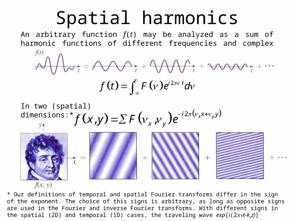
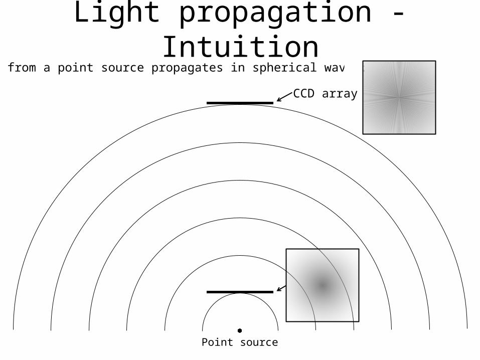
An arbitrary function f(t) may be analyzed as a sum of harmonic functions of different frequencies and complex amplitudes.
In two (spatial) dimensions:*
2, , x yi x y
x yf x y F e
2
i tf t F e d
Spatial harmonics
* Our definitions of temporal and spatial Fourier transforms differ in the sign of the exponent. The choice of this signs is arbitrary, as long as opposite signs are used in the Fourier and inverse Fourier transforms. With different signs in the spatial (2D) and temporal (1D) cases, the traveling wave exp[i(2t-kzz)] represents wave that moves in +z direction as time propagates.

A little on Fourier transform

Example 1
f(x,y)
|F(x,y)|2
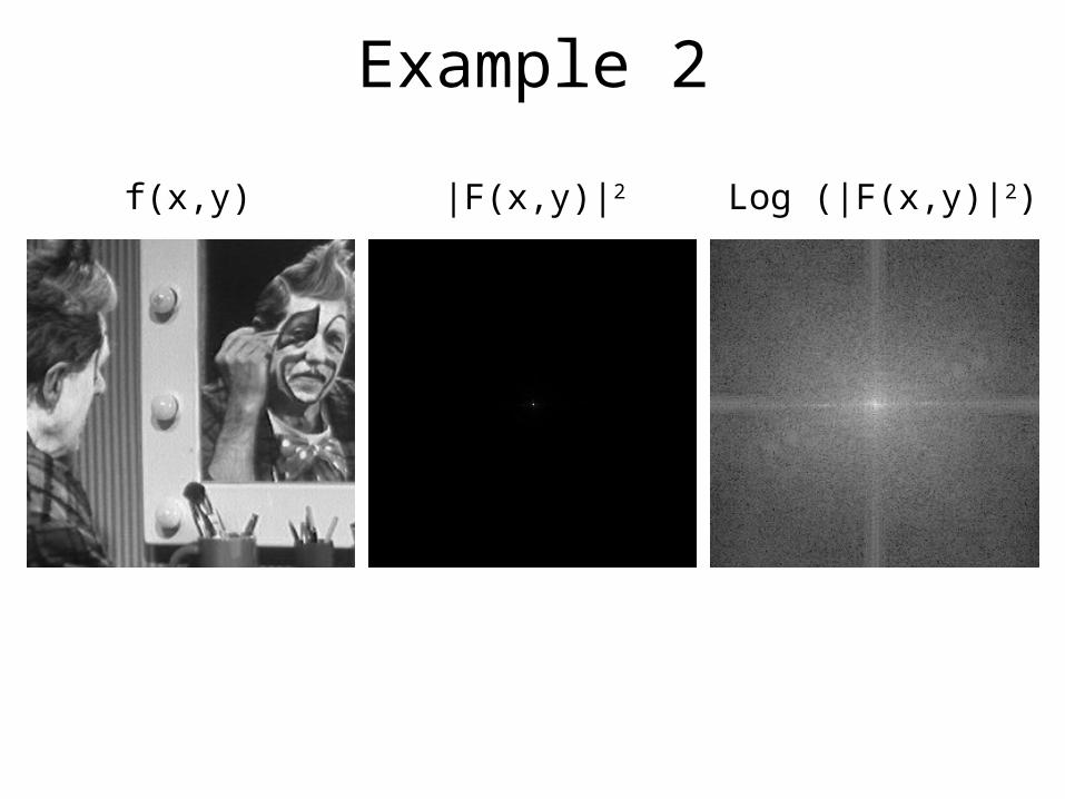
Example 2
f(x,y) |F(x,y)|2 Log (|F(x,y)|2)

Example 3f(x,y) |F(x,y)|2 Log (|F(x,y)|2)
P(x,y)

Example 4
f(x,y) |F(x,y)|2 Log (|F(x,y)|2)

Spatial harmonics & Plane waves , , x y zi k x k y k z
U x y z Ae Consider a plane wave:
(t=0, monochromatic)
with a wavevector
1
1
sin
sin
x x
y y
k k
k k
x = 0 means that there is no component of
k in the x-axis (kx=0).
A: Complex amplitude
2
, ,0
, ,0 ,
x y
x y
i k x k y
i x y
x y
U x y Ae
U x y F eWe also know (previous slides) thatU is comprised of spatial harmonics:
At z=0:
2 2 2
, ,
2.
x y z
x y z
k k k k
k k k k k
This wave propagates at angles:

2
, ,0
, ,0
x y
x y
i k x k y
i x y
U x y Ae
U x y Fe
Spatial harmonics & Plane waves
2
2x x
y y
k
k
→ Spatial frequency [cycles/mm]
→ Optical frequency [cycles/sec]
A single plane wave:
A single spatial harmonic:
, , 2
2
x y x yk
kc
1
1
sin
sin
x x
y y
k k
k k
1
1
sin
sin
x x
y y
(!)
The angles of inclination of the wavevector are then directly proportional to the spatial frequencies of the corresponding harmonic function. Apparently, there is a one-to-one correspondence between the plane wave U(x,y,z) and the harmonic function f(x,y).

Given one, the other can be readily determined, provided the wavelength is known:
- The harmonic function f(x,y) is obtained by sampling at the z0 plane, f(x,y) = U(x,y,z0).
- Given the harmonic function f(x,y), on the other hand, the wave U(x,y,z) is constructed by using the relation:
plane wave U(x,y,z) harmonic function f(x,y)
, , , zik zU x y z f x y e
With:
2 2 2
1 1
1 1
2
sin sin
sin sin
z x y
x x x
y y y
k k k k k
k k
k k
A condition for the validity of this correspondence is that kz is real ( ). This condition implies that x < 1 and y < 1, so that the angles x and y exist.
The signs represent waves traveling in the forward and backward directions. We shall be concerned with forward waves only.
2 2 2 x yk k k
Spatial harmonics & Plane waves
2
2
, , ,
, ,0 ,
x yz z
x y
i x yik z ik z
i x y
U x y z f x y e e e
U x y f x y e
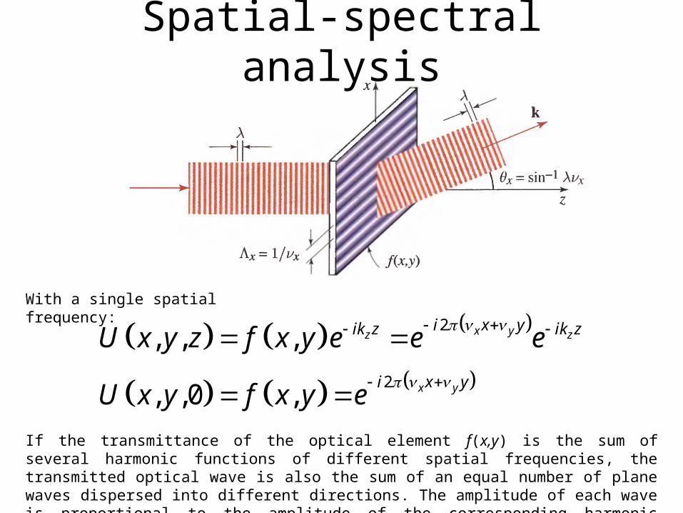
Spatial-spectral analysis
If the transmittance of the optical element f(x,y) is the sum of several harmonic functions of different spatial frequencies, the transmitted optical wave is also the sum of an equal number of plane waves dispersed into different directions. The amplitude of each wave is proportional to the amplitude of the corresponding harmonic component of f(x,y).
With a single spatial frequency:

Mathematically, if f(x,y) is a superposition integral of harmonic functions,
with frequencies x and y, and amplitudes F(x,y), the transmitted wave U(x,y,z) is the superposition of plane waves,
2, ,
x yi x y
x y x yf x y F e d d
2, , ,
x y zi x y ik z
x y x yU x y z F e e d d
2 2 2 2 2 2=2 . z x y x yk k k kwith complex envelopes F(x ,y) and
2
2
, ,
, ,
x y
x y
i x y
x y x y
i x y
x y
f x y F e d d
F f x y e dxdy
Spatial-spectral analysis
For any z:

A thin optical element of complex amplitude transmittance f(x,y) decomposes an incident plane wave into many plane waves. Each wave travels at angles x = sin-1(x) and y = sin-1(y) and has a complex envelope F(x,y).
Spatial-spectral analysis
This process of "spatial spectral analysis" is analogous to the angular dispersion of different temporal-frequency components (wavelengths) by a prism. Free-space propagation serves as "spatial prism“, sensitive to the spatial rather than temporal frequencies of the waves.

The transfer functioninput plane output plane
, , ,g x y U x y d , , ,0f x y U x y
We regard f(x,y) and g(x,y) as the input and output of a linear system. The system is linear since the Helmholtz equation, which U(x,y,z) must satisfy, is linear.

Shift-invariant system: Invariance of free space to displacement of the coordinate system.
A linear shift-invariant system is characterized by its impulse response function h(x,y) or by its transfer function H(x,y).
Linear systems
Transfer function
Impulse response

Transfer function of free space
2 2, ,
x y x yi x y i x y
x y x yf x y F e d d A e
consider a single harmonic input function,
which corresponds to a plane wave: , , x y zi k x k y k z
U x y z A e
2 2 2 2 2 2=2 z x y x yk k k kwhere:
, x y zi k x k y k d
g x y A e
2 2 22,,
,
x yzi dik d
x y
g x yH e e
f x y
Thus transfer function of free space:
After propagating a distance d:
2
2
x x
y y
k
k

Transfer function of free space
2 2 22,
x yi d
x yH e
The (complex) transfer function of free space:
sphere

Fourier optics and imaging
•Linear optical systems
•Fresnel diffraction
•Fraunhofer diffraction
•The lens
•Optical resolution

Fresnel approximation
If the input function f(x,y) contains only spatial frequencies that are much smaller than the cutoff frequency -1, so that
the plane wave components of the propagating light then make small angles xx and yy , corresponding to paraxial rays.
2 2 22,
x yi d
x yH e
2 2 2 , x y
2 22 2
2 2 2 22
2 2
2 12 12 2,
,
x yx y
x y
x y
dd iii d
x y
i dikdx y
H e e e
H e e
1 1 2
*
*
sphere
parabola

Given the input function f(x,y), the output function g(x,y) may be determined as follows:
1. we determine the Fourier transform
Input-output relation (Fresnel)
2, ,
x yi x y
x yF f x y e dxdy
2. the product H(x,y) F(x,y) gives the complex envelopes of the plane wave components in the output plane.
3. the complex amplitude in the output plane is the sum of the contributions of these plane waves:
2, , ,
x yi x y
x y x y x yg x y H F e d d
Using the Fresnel approximation for H(x,y), we have: 2 2
, x yi dikd
x yH e e
2 2 2, ,
x y x yi d i x yikdx y x yg x y e F e e d d

Impulse response of free spaceThe impulse response function h(x,y) of the system of free-space propagation is the response g(x,y) when the input f(x,y) is a point at the origin (0,0).
2, 1 ,
x yi x y
x y x yg x y H e d d
2 2, , , 1
x y x yi x y i x y
x yF f x y e dxdy x y e dxdy
which is the inverse Fourier transform of (exercise):
2 2
2, ,
x yikikd di
h x y g x y e ed
Thus, each point in the input plane generates a paraboloidal wave; all such waves are superimposed at the output plane.
2 2
, x yi dikd
x yH e e

Free space propagation as a convolution (Fresnel)
Knowing h, we can regard f(x,y) as a superposition of different points (delta functions), each producing a paraboloidal wave.
The wave originating at the point (x’,y’) has an amplitude f(x’,y’) and is centered about (x’,y’) so that it generates a wave with amplitude f(x’,y’)h(x-x’,y-y’) at the point (x,y) in the output plane. The sum of these contributions is the two-dimensional convolution:
, , , ,
g x y f x y h x x y y dx dy
which in the Fresnel approximation becomes:
2 2
, , .
x x y y
iikd dig x y e f x y e dx dy
d
Unlike previous derivation of g from f, here no Fourier transform is involved.
2 2
2,
x yikikd di
h x y e ed

f h f g t d
Convolution

Fresnel approximation: summary
2 2
, ,
x x y y
iikd dig x y e f x y e dx dy
d
2 2 2, ,
x y x yi d i x yikdx y x yg x y e F e e d d
Within the Fresnel approximation, there are two approaches for determining the complex amplitude g(x,y) in the output plane, given the complex amplitude f(x,y) in the input plane:
1. space-domain approach in which the input wave is expanded in terms of paraboloidal elementary waves.
2. frequency-domain approach in which the input wave is expanded as a sum of plane waves:

Fourier optics and imaging
•Linear optical systems
•Fresnel diffraction
•Fraunhofer diffraction
•The lens
•Optical resolution

Fraunhofer approximation
2 2
2 2 2 2 2
, ,
,
x x y yiikd d
x y x y xx yyiikd d
ig x y e f x y e dx dy
d
ie f x y e dx dy
d
Start with the space-domain approach of Fresnel approximation:
If f(x,y) is confined to a small area of radius b, and if the distance d is sufficiently large so that b2/d is small, then the phase factor is negligible: 2 2 x y d
2 2
2 2
2 2
2
2
, ,
,
,
x y
x y xx yyi iikd d d
x yi i x yikd d
x yiikd d
ig x y e e f x y e dx dy
d
ie e f x y e dx dy
d
i x ye e F
d d d
x
y
x
dy
d
1sin
sin
sin tan
x x
x x
x x x x
x x
d d

In the Fraunhofer approximation, the complex amplitude g(x,y) of a wave of wavelength in the z=d plane is proportional to the Fourier transform F(x,y) of the complex amplitude f(x,y) in the z=0 plane, evaluated at the spatial frequencies x =x/d and y =y/d.
The approximation is valid if f(x,y) at the input plane is confined to a circle of radius b satisfying:
Fraunhofer approximation
2 2
0 0, ,
x yiikd dx y i
g x y h F h e ed d d
“Fraunhofer region”
Fresnel region
Fraunhofer region2b
2 2
max
2
2
2
x yd
bd
,f x y ,g x y

Two slits. The width of the silts is constant and the distance between them is varied.
One slit. The width of the silts is varied.
Fraunhofer – FT in the far-field
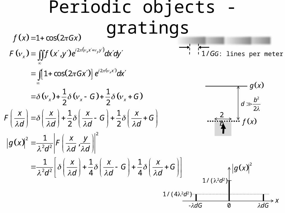
Periodic objects - gratings
G: lines per meter
2
2
22
2 2
2 2
1 cos 2
,
1 cos 2
1 1
2 21 1
2 2
1,
1 1 1
4
x y
x
i x y
x
i x
x x x
f x Gx
F f x y e dx dy
Gx e dx
G G
x x x xF G G
d d d d
x yg x F
d d d
x xG
d d d 4
xG
d
1/G
dGx
-dG 0
1/(2d2)
1/(42d2)
2g x
2b
2
2
b
d
g x
f x


http://highered.mcgraw-hill.com/sites/0072495855/student_view0/chapter10/animation__sarcomere_contraction.html
Sarcomere contractionsSarcomeres are multi-protein complexes composed of different filament systems.
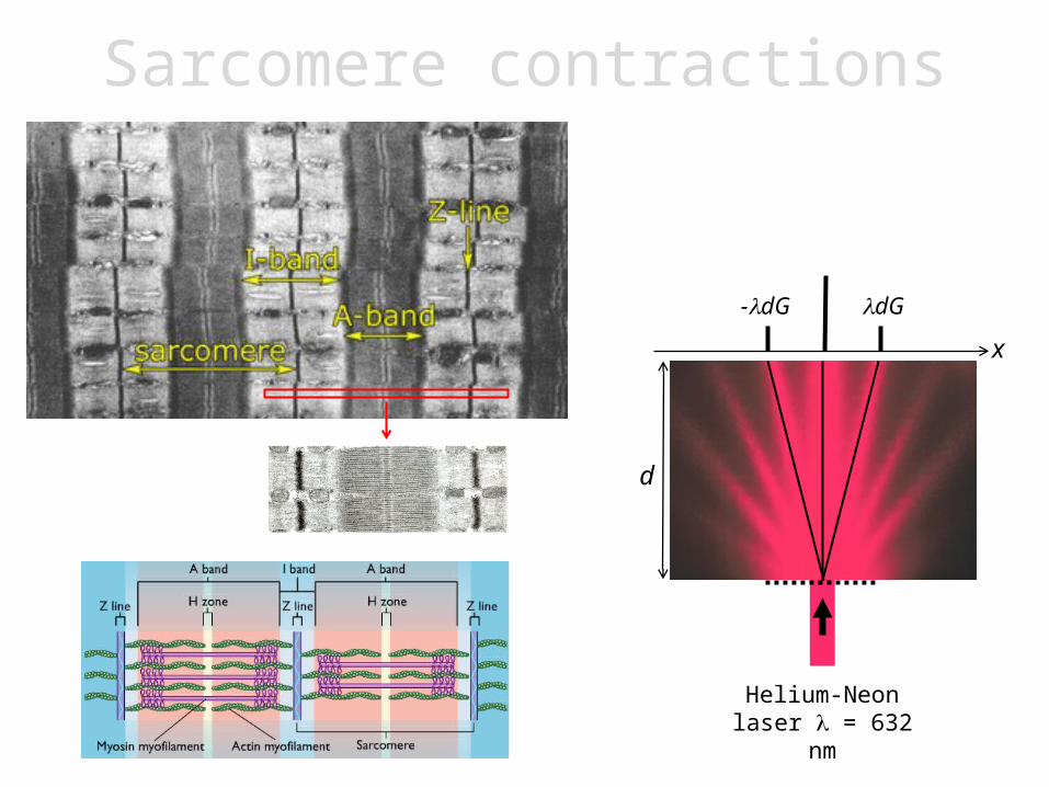
Sarcomere contractions
d
dG-dG
Helium-Neon laser = 632 nm
x

Fourier optics and imaging
•Linear optical systems
•Fresnel diffraction
•Fraunhofer diffraction
•The lens
•Optical resolution

Angular spectrum - definition
2
2
, , , ,
, , , ,
x y
x y
i x y
x y
i x y
x y x y
A z U x y z e dxdy
U x y z A z e d d
Definition: The angular spectrum A(x,y,z) of a wave U(x,y,z) emerging from an object:
AU FT pair:
Thus A(x,y,z) is simply the equivalent for the Fourier transform F of the object f(x,y):
, , ,
, , ,
z
z
ik zx y x y
ik z
A z F e
U x y z f x y e
Object complex transmissionComplex wave
Fourier transform of the objectAngular spectrum

Substitute into Helmholtz equation
And executing the derivatives of the x and y coordinates gives:
Propagation of angular spectrum
with a solution:
2 2 2 2 2 2 2
2 2 2
4 1
11
2
, , , ,0 , ,0
, ,0
x y x y
x y
iz k izk
x y x y x y
izk
x y
A z A e A e
A e
2 2
, , , ,0 x yi zikz
x y x yA z A e e
Propagation of the angular spectrum (Fresnel approximation)
2
2 2 2 22
4 0 x y
d Ak A
dz
2 2 2
1 1 2
x yFresnel approximation:
2 2, , , , 0U x y z k U x y z
222 2 2 2
2, , 4 , , 0
x yi x y
x y x y x y x y
dA z k A z e d d
dz= 0
Which yields a differential equation:
2, ,
x yi x y
x y x yU A z e d d
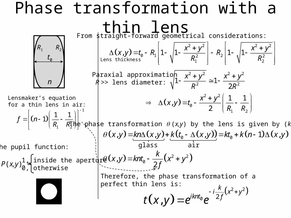
Phase transformation with a thin lens
Therefore, the phase transformation of a perfect thin lens is:
2 2
0 2,
k
i x yiknt ft x y e e
1, inside the aperture0, otherwise
2 2 2 2
0 1 22 21 2
, 1 1 1 1
x y x yx y t R R
R R
2 2 2 2
2 21 1
2
x y x y
R R
Paraxial approximation R >> lens diameter:
2 2
01 2
1 1 ,
2
x yx y t
R R
The phase transformation (x,y) by the lens is given by (k=2/):
0 0, , , 1 , x y kn x y k t x y kt k n x y
1
1 2
1 11
f nR R
2 20,
2
kx y knt x y
f
The pupil function:
From straight-forward geometrical considerations:
glass air
P(x,y) =
Lens thicknesst0
n
R1 R2
Lensmaker’s equation for a thin lens in air:

2 2
2 2 2 2
2 22 2 2 2
2
2 2
222 2
, , , ,0
, ,0
, ,0 ,
, ,
x x y yiikz z
k ki xx yyi x y i x yikz zz z
kk ki x y i xx yyi x y i x yikz f zz z
iU x y z e U x y e dx dy
z
ie e U x y e e dx dy
z
ie e U x y P x y e e e dx dy
z
U x y
2 2
2 2
2
2
22
, ,0 ,
, ,0 ,
x y
ki x y i xx yy
ikf f f
ki x y i x yikf f
if e e U x y P x y e dx dy
f
ie e U x y P x y e dx dy
f
Fraunhofer diffraction by a lensThe field after a (thin) lens (neglecting the exp(iknt0) term):
2 2
2, ,0 , ,0 ,k
i x yfU x y U x y P x y e
f
, ,0U x y , ,0U x y
, ,U x y f
Using the Fresnel integral:
x
y
x
f
y
fLens Fraunhofer diffraction of U(x,y,0-) multiplied by the pupil function
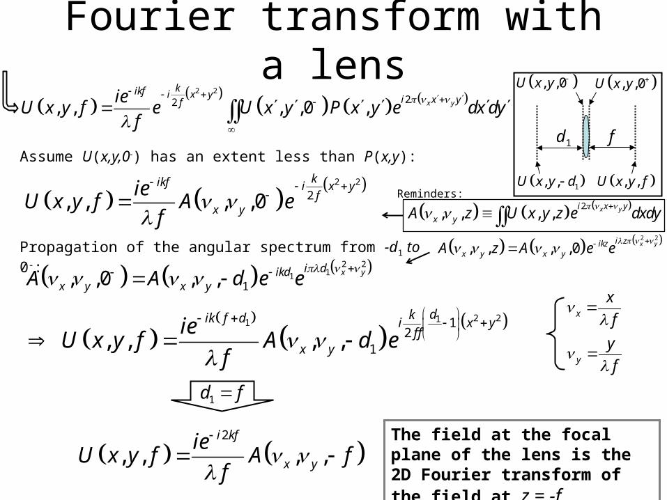
Fourier transform with a lens , ,0U x y , ,0U x y
d1
1, ,U x y d , ,U x y f
2 211
1, ,0 , , x yi dikd
x y x yA A d e e
2 2
2, , , ,0
kikf i x yf
x y
ieU x y f A e
f
Assume U(x,y,0-) has an extent less than P(x,y):
2 211 12
1 , , , ,
dkik f d i x yf f
x y
ieU x y f A d e
f
2
, , , ,
i kf
x y
ieU x y f A f
f
The field at the focal plane of the lens is the 2D Fourier transform of the field at z = -f
f
Propagation of the angular spectrum from -d1 to 0-:
1d f
x
y
x
f
y
f
2, , , ,
x yi x y
x yA z U x y z e dxdyReminders:
2 2
, , , ,0 x yi zikz
x y x yA z A e e
2 222, , , ,0 ,
x y
kikf i x y i x yfieU x y f e U x y P x y e dx dy
f

2
, ,
i kfie x yg x y F
f f f
Fourier transform property of a lens:
The complex amplitude of light at a point (x,y) in the back focal plane of a lens of focal length f is proportional to the Fourier transform of the complex amplitude in the front focal plane evaluated at the frequencies x/λf, y/λf. This relation is valid in the Fresnel approximation. Without the lens, the Fourier transformation is obtained only in the Fraunhofer approximation, which is more restrictive.
Fourier transform with a lens
, , ,
, , ,
z
z
ik zx y x y
ik z
A z F e
U x y z f x y e
2
, , , ,
i kf
x y
ieU x y f A f
f

2 2
, , ,
,
ikd i x x y y
d
g x y f x y h x x y y dx dy
ief x y e dx dy
d
, ,0U x y , ,0U x y
d1
1, , U x y d , ,i i iU x y d
di
Assume a positive, aberration-free thin lens and monochromatic light. Free space propagation as a convolution (Fresnel):
To find h, we replace f(x’,y’) U(x,y,-d1) (x-x1,y-y1,-d1):
2 22 21 1
1
2 2
2 2
2 2
1
21 1 1
2
21 1
1 1 1
2
, ,0 , ,
, ,0 , ,0 ,
, , , , , , ,0
,
i i
i
i
ii
x x y yx x y yikz iki dz
ki x y
f
ki x x y y
di i i i i
xk iki x ydd d f
ieU x y x x y y d e dx dy e
z
U x y U x y P x y e
U x y d h x y x y U x y e dxdy
P x y e e1 1
1 1
i
i
yx yx y
d d d dxdy
Image formation with a lens
1 1,x y

1 1
1 1
2
1 1
2
1 1
, , , ,
,
i ii
i i
i x Mx x y My yd
i i
x yi x x y y
M M
i i
h x y x y P x y e dxdy
e dxdy
x yx y
M M
1
idM
d
1 11 , , , ,
i i i
x yU x y d U d
M M
Magnification
Neglect P(x,y):
2
i xxe dx x
• Inversion• Magnification
1
1 1 1
id f dThe lens law
1 12 2
1 11
1 1 1
2,
i i
i ii
x yx yk ik x yi x yd d d dd d fh P x y e e dxdy
=0
In this case, the impulse response becomes
Imaging by a lens:
Image formation with a lens , ,0U x y , ,0U x y
d1
1, , U x y d , ,i i iU x y d
di
1 1,x y

Imaging examples ,U x y ,U x y
f f f f
,U x y ,U x y
f f f f
,x y
Af f
,U x y ,4 4
x yU
f f f f f f1
idM
d
1
1 1 1
id f d
The lens law
Magnification
1
5
5 4
id f
d f
1
2
2
id f
d f
,U x y ,2 2
x yU
f1 f1 f2 f2
,x y
Af f
2
1
f
Mf
f2=2ff1
F
F
F
F
F
F
F
F
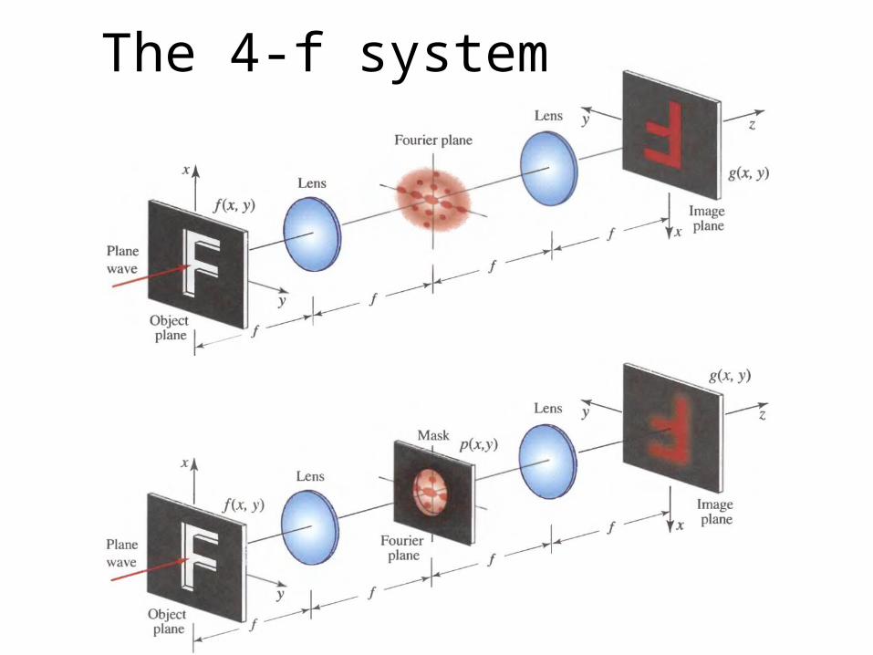
The 4-f system

,U x y ,U x y
f f f f
, x yA
Imaging examples
Image (inverted)Object Mask

Fourier optics and imaging
•Linear optical systems
•Fresnel diffraction
•Fraunhofer diffraction
•The lens
•Optical resolution

Point-spread function (PSF)
Perfect spherical wave
Diffraction limited (also “Fourier limited”) system:
PSF ↔ Impulse response
Point object Image
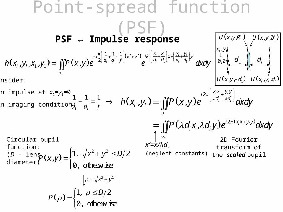
1 12 2
1 11
1 1 1
21 1, , , ,
i i
i ii
x yx yk ik x yi x yd d d dd d f
i ih x y x y P x y e e dxdy
2
2
, ,
,
i i
i i
i i
x x y yi
d di i
i x x y yi i
h x y P x y e dxdy
P d x d y e dxdy
Consider:
• An impulse at x1=y1=0
• An imaging condition: 1
1 1 1
id d f
PSF ↔ Impulse response
2D Fourier transform of the scaled pupil
2 2x y
Circular pupil function:(D - lens diameter)
2 21, 2
,0, otherwise
x y DP x y
1, 2
0, otherwise
DP
x’=x/λdi
(neglect constants)
, ,0U x y , ,0U x y
d1
1, , U x y d , ,i i iU x y d
di
1 1,
0,0
x y
Point-spread function (PSF)

id
1
1
2
2
, 0,0
i
i
JFT P
DJ
dh x y h
Dd
xi
yi
“Airy disk”
2h
PSF
1.22 is
d
D
1.22 is
d
D
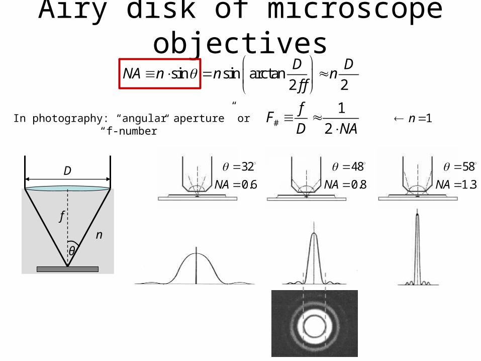
Airy disk of microscope objectives
58
1.3
NA
48
0.8
NA
32
0.6
NA
θn
#
sin sin arctan2 2
1
2
D DNA n n n
f f
fF
D NA
D
In photography: “angular aperture” or “f-number” 1 n
f

Gaussian beams - propertiesBeam divergence
2
00
0
0
0 00 2
0 0 0
1
zW z W
z
WW z z
z
W W
z W W
0 z z
Thus the total angle is given by 00
42
2W
2 2
2 200
ikz ik i zW z R zW
U r A e eW z
2
00
2
0
1
0
00
1
1
tan
zW z W
z
zR z z
z
zz
z
zW
0 0
42 2
W
Reminder
00
sin
NA n n
W
NA for Gaussian beams
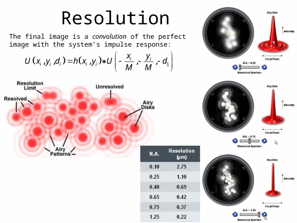
ResolutionThe final image is a convolution of the perfect image with the system’s impulse response:
1, , , , ,
i ii i i i i
x yU x y d h x y U d
M M

f h f g t d
Convolution

2D convolution examples

Quantifying resolution The Rayleigh criterion

Rayleigh criterion
1sin 1.22 r D
1.22
10.61
fl
D
lNA
For an ideal lens:
“Two point sources are just resolved if they have an angular separation equal to the angular radius of the Airy disk.”
For a microscope objective:sin
2
DNA n n
f

Effect of noise on resolution

2 2
, , , ,0
i i
ikz i x x y yz
i i
ieU x y z U x y e dxdy
z
SummaryAn arbitrary wave may be analyzed as a superposition of plane waves.
U(x,y,0)=f(x,y)e-ikz can be represented as a combination of spatial harmonics:
Fraunhofer approximation
Propagation of the angular spectrum
Fresnel approximation
The 4-f system allows Fourier domain image manipulations
2 2
, , , ,0 x yi zikz
x y x yA z A e e
The PSF of a lens is limited by its pupil function
2 2
2, , , ,0
i i
kikzi x y
zi i
ieU x y z e FT U x y
z
1.22 is
d
D
At its focal plane a lens performs a Fourier transform of the incoming field
2
, ,
i kfie x yg x y F
f f f