19878 29W p001-034 - Cengage · TIME VALUE OF MONEY Time value concepts, ... For a more detailed review of time value of money concepts, see Web Chapter 28 ... 19878_29W_p001-034.qxd

29C H A P T E R

29W-1

Basic Financial Tools: A Review

IMA

GE

:©G

ET

TY

IM

AG

ES

, IN

C.,

PH

OTO

DIS

C C

OLL

EC

TIO

N

The building blocks of finance include the time value of money, risk and its relationship withrates of return, and stock and bond valuation models. These topics are covered in introductoryfinance courses, but because of their fundamental importance, we review them in this Webchapter.1

TIME VALUE OF MONEY

Time value concepts, or discounted cash flow analysis, underlie virtually all theimportant topics in financial management, including stock and bond valuation,capital budgeting, cost of capital, and the analysis of financing vehicles such asconvertibles and leasing. Therefore, an understanding of time value concepts isessential to anyone studying financial management.

Future ValuesAn investment of PV dollars today at an interest rate of i percent for n periodswill grow over time to some future value (FV). The following time line shows howthis growth occurs:

1This review is limited to material that is necessary to understand the chapters in the main text. For a more detailed treatment of risk, return, and valuation models, see Chapters 2 through 5. For a more detailed review of time value ofmoney concepts, see Web Chapter 28.

= FV2(1 + i)= FV1(1 + i)= PV(1 + i)

0 i% 1 n – 1

PV FV1 FV2 FV3 FVn – 1 FVn

n

= FVn – 2(1 + i) = FVn – 1(1 + i)

2 3

19878_29W_p001-034.qxd 3/14/06 4:30 PM Page 1

29W-2 • Web Chapter 29 Basic Financial Tools: A Review

2See the Web Extension to Chapter 5 for a derivation of the sum of a geometric series.3An annuity in which payments are made at the start of the period is called an annuity due. The future value interestfactor of an annuity due is (1 � i)FVIFAi,n.

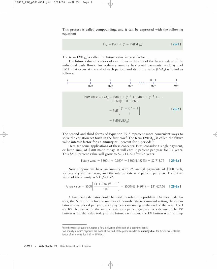
This process is called compounding, and it can be expressed with the followingequation:

FVn � PV(1 � i)n � PV(FVIFi,n) | 29-1 |

The term FVIFi,n is called the future value interest factor.The future value of a series of cash flows is the sum of the future values of the

individual cash flows. An ordinary annuity has equal payments, with symbolPMT, that occur at the end of each period, and its future value (FVAn) is found asfollows:

0 1 n – 1 n2

PMT PMT PMT PMTPMT

3

| 29-2 |

� PMT(FVIFAi,n)

The second and third forms of Equation 29-2 represent more convenient ways tosolve the equation set forth in the first row.2 The term FVIFAi,n is called the futurevalue interest factor for an annuity at i percent for n periods.3

Here are some applications of these concepts. First, consider a single payment,or lump sum, of $500 made today. It will earn 7 percent per year for 25 years.This $500 present value will grow to $2,713.72 after 25 years:

Future value � $500(1 � 0.07)25 � $500(5.42743) � $2,713.72 | 29-1a |

Now suppose we have an annuity with 25 annual payments of $500 each,starting a year from now, and the interest rate is 7 percent per year. The futurevalue of the annuity is $31,624.52:

| 29-2a |

A financial calculator could be used to solve this problem. On most calcula-tors, the N button is for the number of periods. We recommend setting the calcu-lator to one period per year, with payments occurring at the end of the year. The I(or I/Y) button is for the interest rate as a percentage, not as a decimal. The PVbutton is for the value today of the future cash flows, the FV button is for a lump

Future value � $500 c (1 � 0.07) 25 � 1

0.07d � $500 (63.24904) � $31,624.52

Future value � FVAn � PMT(1 � i)n�1 � PMT(1 � i)n�2 � . . .

� PMT(1� i) � PMT

� PMT c (1 � i ) n � 1

id

19878_29W_p001-034.qxd 3/14/06 4:30 PM Page 2

Web Chapter 29 Basic Financial Tools: A Review • 29W-3

4Our Technology Supplement contains tutorials for the most commonly used financial calculators (about 12 typewrittenpages versus much more for the calculator manuals). Our tutorials explain how to do everything needed in this book. Seeour Preface for information on how to obtain the Technology Supplement.5The present value interest factor for an annuity due is (1 � i)PVIFAi,n.

| 29-3 |

| 29-4 |

sum cash flow at the end of N periods, and the PMT button is used if we have aseries of equal payments that occur at the end of each period. On some calculatorsthe CPT button is used to compute present and future values, interest rates, andpayments. Other calculators have different ways to enter data and find solutions,so be sure to check your specific manual.4 To find the future value of the singlepayment in the example above, input N � 25, I � 7, PV � �500 (negativebecause it is a cash outflow), and PMT � 0 (because we have no recurring pay-ments). Press CPT and then the FV key to find FV � $2,713.72. To calculate thefuture value of our annuity, input N � 25, I � 7, PV � 0, PMT � �500, andthen press CPT and then the FV key to find FV � $31,624.52. Some financial cal-culators will display the negative of this number.

Present ValuesThe value today of a future cash flow or series of cash flows is called the presentvalue (PV). The present value of a lump sum future payment, FVn, to be receivedin n years and discounted at the interest rate i, is

PVIFi,n is the present value interest factor at i percent due in n periods.The present value for an annuity is the sum of the present values of the indi-

vidual payments. Here are the time line and formula for an ordinary annuity:

� FVn (PVIFi,n )

PV � FVn

1

(1 � i ) n

0 1 n – 1 n2

PMT PMT PMT PMTPMT

3

� PMTC 1 �

1

(1 � i ) n

i

S Present value � PVAn �

PMT

(1 � i )�

PMT

(1 � i ) 2� p �

PMT

(1 � i ) n�1�

PMT

(1 � i ) n

� PMT(PVIFAi,n)

PVIFAi,n is the present value interest factor for an annuity at i percent for n periods.5

19878_29W_p001-034.qxd 3/14/06 4:30 PM Page 3


| 29-4a |

The present value of a $500 lump sum to be received in 25 years when theinterest rate is 7 percent is $500/(1.07)25 � $92.12. The present value of a seriesof 25 payments of $500 each discounted at 7 percent is $5,826.79:

PV � $500 £1 �

1

(1.07) 25

0.07

≥� 500 (11.65358)

� $5,826.79

Present values can be calculated using a financial calculator. For the lump sumpayment, enter N � 25, I � 7, PMT � 0, and FV � �500, and then press CPT andthen the PV key to find PV � $92.12. For the annuity, enter N � 25, I � 7, PMT� �500, and FV � 0, and then press CPT and then the PV key to find PV �$5,826.79.

Present values and future values are directly related to one another. We sawjust above that the present value of $500 to be received in 25 years is $92.12. Thismeans that if we had $92.12 now and invested it at a 7 percent interest rate, itwould grow to $500 in 25 years. For the annuity example, if you put $5,826.79in an account earning 7 percent, then you could withdraw $500 at the end of eachyear for 25 years, and have a balance of zero at the end of 25 years.

An important application of the annuity formula is finding the set of equalpayments necessary to amortize a loan. In an amortized loan (such as a mortgageor an auto loan) the payment is set so that the present value of the series of pay-ments, when discounted at the loan rate, is equal to the amount of the loan:

Loan amount � PMT(PVIFAi,n), orPMT � (Loan amount)/PVIFAi,n

Each payment consists of two elements: (1) interest on the outstanding balance(which changes over time) and (2) a repayment of principal (which reduces theloan balance). For example, consider a 30-year, $200,000 home mortgage withmonthly payments and a nominal rate of 9 percent per year. There are 30(12) �360 monthly payments, and the monthly interest rate is 9%/12 � 0.75%. Wecould use Equation 29-4 to calculate PVIFA0.75%,360, and then find the monthlypayment, which would be

PMT � $200,000/PVIFA0.75%,360 � $1,609.25

It would be easier to use a financial calculator, entering N � 360, I � 0.75, PV ��200000, and FV � 0, and then press CPT and then the PMT key to findPMT � $1,609.25.

To see how the loan is paid off, note that the interest due in the first month is0.75 percent of the initial outstanding balance, or 0.0075($200,000) � $1,500.00.Since the total payment was $1,609.25, then $1,609.25 � $1,500.00 � $109.25 isapplied to reduce the principal balance. At the start of the second month the out-standing balance would be $200,000 � $109.25 � $199,890.75. The interest onthis balance would be 0.75 percent of the new balance or 0.0075($199,890.75) �$1,499.18, and the amount applied to reduce the principal would be $1,609.25 �

19878_29W_p001-034.qxd 3/14/06 4:30 PM Page 4


$1,499.18 � $110.07. This process would be repeated each month, and the result-ing amortization schedule would show, for each month, the amount of the paymentthat is interest and the amount applied to reduce principal. With a spreadsheet pro-gram such as Excel, we can easily calculate amortization schedules.

Nonannual CompoundingNot all cash flows occur once a year. The periods could be years, quarters,months, days, hours, minutes, seconds, or even instantaneous periods.

Discrete Compounding The procedure used when the period is less than ayear is to take the annual interest rate, called the nominal, or quoted rate, anddivide it by the number of periods in a year. The result is called the periodic rate.In the case of a monthly annuity with a nominal annual rate of 7 percent, themonthly interest rate would be 7%/12 � 0.5833%. As a decimal, this is 0.005833.Note that interest rates are sometimes stated as decimals and sometimes as per-centages. You must be careful to determine which form is being used.

When interest is compounded more frequently than once a year, interest willbe earned on interest more frequently. Consequently, the effective rate will exceedthe quoted rate. For example, a dollar invested at a quoted (nominal) annual rate of7 percent but compounded monthly will earn 7/12 � 0.5833 percent per month for12 months. Thus, $1 will grow to $1(1.005833)12 � 1.0723 over one year, or by7.23%. Therefore, the effective, or equivalent, annual rate (EAR) on a 7 percentnominal rate compounded monthly is 7.23 percent.

If there are m compounding intervals per year and the nominal rate is iNom,then the effective annual rate will be

| 29-5 |

The larger the value of m, the greater the difference between the nominal andeffective rates. Note that if m � 1, which means annual compounding, then thenominal and effective rates are equal.6

EAR (or EFF% ) � a 1 �iNom

mb

m

� 1.0

6For some purposes it is appropriate to use instantaneous, or continuous, compounding. Equation 29-5 can be used forany number of compounding intervals, m, per year: m � 1 (annual compounding), m � 2 (semiannual compounding),m � 12 (monthly compounding), m � 365 (daily compounding), m � 365(24) � 8,760 (hourly compounding), andeven more frequently. As m approaches infinity, the compounding interval approaches zero, and the compoundingbecomes instantaneous, or continuous. The EAR for continuous compounding is given by the following equation:

EARcontinuous � eiNom � 1.0 | 29-5a |

Here e is approximately equal to 2.71828; most calculators have a special key for e. The EAR of a 7 percent investmentcompounded continuously is e0.07 � 1.0 � 0.0725 � 7.25%.

Equation 29-5a can also be used to find the future value of a payment invested for n years at a rate inom

compounded continuously:

FVn � PV(eiNomn) | 29-1a |

Similarly, the present value of a future sum to be received in n periods discounted at a nominal rate of inom compoundedcontinuously is found using this equation:

| 29-2a |PV �FVn

eiNomn� FVn (e�iNomn )

19878_29W_p001-034.qxd 3/14/06 4:30 PM Page 5


0 1 1 202

PMT PMTYou need$912,855

on this date

–100,000 –100,000PMT

480 2

–100,000

Months untilretirement Years after retirement

Solving for the Interest RateThe general formula for the present value of a series of cash flows, CFt, discountedat some rate i, is as follows:

| 29-6 |

The cash flows can be equal, in which case CFt � PMT � constant, so we have anannuity, or the CFt can vary from period to period. Now suppose we knowthe current price of the asset, which is by definition the PV of the cash flows, andthe expected cash flows themselves, and we want to find the rate of return on theasset, or its yield. The asset’s expected rate of return, or yield, is defined to be thevalue of i that solves Equation 29-6. For example, suppose you plan to finance acar that costs $22,000, and the dealer offers a five-year payment plan thatrequires $2,000 down and payments of $415.17 per month for 60 months. Sinceyou would be financing $20,000 over 60 months, the monthly interest rate on theloan is the value of i that solves Equation 29-4a:

$20,000 � 415.17(PVIFAi,60) | 29-4a |

This equation would be difficult to solve by hand, but it is easy with a financialcalculator. Enter PV � 20000, PMT � �415.17, FV � 0, and N � 60, and pressCPT and then the I key to find I � 0.75, or 3/4 percent a month. The nominalannual rate is 12(0.0075) � 0.09 � 9%, and the effective annual rate is(1.0075)12 � 1 � 9.38%.

Complex Time Value ProblemsThe present and future value equations can be combined to find the answers tomore complicated problems. For example, suppose you want to know how muchyou must save each month to retire in 40 years. After retiring, you plan to withdraw$100,000 per year for 20 years, with the first withdrawal coming one year afterretirement. You will put away money at the end of each month, and you expect toearn 9 percent on your investments. Here is a diagram of the problem:

PV �CF1

(1 � i )�

CF2

(1 � i ) 2� p �

CFn

(1 � i ) n� a

n

t�1

CFt

(1 � i ) t

The solution requires two steps. First, you must find the amount needed to fundthe 20 retirement payments of $100,000. This amount is found as follows: PV �$100,000(PVIFA9%,20) � $100,000(9.12855) � $912,855. Therefore, you must

19878_29W_p001-034.qxd 3/14/06 4:30 PM Page 6


accumulate $912,855 by the 40(12) � 480th month if you are to make the 20withdrawals after retirement. Each of the 480 deposits will earn 9%/12 � 0.75%per month. The second step is to find your required monthly payment. Thisinvolves finding the PMT stream that grows to the required future value, and it isfound as follows:

FV � $912,855 � PMT(FVIFA0.75%,480) � PMT(4,681.32)PMT � $912,855/4,681.32 � $195.00 per month7

The problem could also be solved with a financial calculator. First, to calculatethe present value of the 20 payments of $100,000 at an annual interest rate of9 percent, enter N � 20, I � 9, PMT � �100000, and FV � 0, and then press CPTand then the PV key to find PV � $912,855. Second, clear the calculator and thenenter FV � 912855, N � 480, PV � 0, and I � 9/12, and then press CPT andthen the PMT key to find PMT � �195.00, which is the monthly investmentrequired to accumulate a balance of $912,855 in 40 years. Note that the $912,855is both a present value and a future value in this problem. It is a present valuewhen finding the accumulated amount required to provide the post-retirementwithdrawals, but it is a future value when used to find the pre-retirement payments.

What is compounding? How is compounding related to discounting?Explain how financial calculators can be used to solve present value and future value

problems.What is the difference between an ordinary annuity and an annuity due?Why is semiannual compounding better than annual compounding from a saver’s standpoint?

What about from a borrower’s standpoint?Define the terms “effective (or equivalent) annual rate,” “nominal interest rate,” and “periodic

interest rate.”How would one construct an amortization schedule?

BOND VALUATION

Finding the value of a bond is a straightforward application of the discountedcash flow process. A bond’s par value is its stated face value, which is the amountthe issuer must pay to the bondholder at maturity. We assume a par value of$1,000 in all our examples, but it is possible to have any value that is a multipleof $1,000. The coupon payment is the periodic interest payment that the bond

7For simplicity we have assumed that your retirement funds will earn 9 percent compounded monthly during the accumu-lation phase and 9 percent compounded annually during the withdrawal phase. It is probably more realistic to assumethat your earnings will be compounded the same during both phases. In that case you would use the effective annualrate for 9 percent compounded monthly, which is 9.38 percent, as the annual interest rate during the withdrawal phase.This larger effective rate would reduce the amount you need to save by the time you retire to $888,620, and yourmonthly contribution would be $189.82.

Note also that it is relatively easy to solve problems such as this with a spreadsheet program such as Excel. More-over, with a spreadsheet model, you could make systematic changes in variables such as the interest rate earned, years toretirement, years after retirement, and the like, and determine how sensitive the monthly payments are to changes inthese variables. This is especially useful to financial planners.

Self-Test Questions

19878_29W_p001-034.qxd 3/14/06 4:30 PM Page 7


8By convention, annual coupon rates and market interest rates on bonds are quoted at two times their six-month rates.So, a $1,000 bond with a $45 semiannual coupon payment has a nominal annual coupon rate of 9 percent.

provides. Usually these payments are made every six months (semiannual pay-ments), and the total annual payment as a percentage of the par value is called thecoupon interest rate. For example, a 15-year, 8 percent coupon, $1,000 par valuebond with semiannual payments calls for a $40 payment each six months, or $80per year, for 15 years, plus a final principal repayment of $1,000 at maturity. Atime line can be used to diagram the payment stream:

0.5 yearYear

0 1 3 28 29 300 0.5 1.0 1.5 14 14.5 15

$40 $40 $40 $40 $40 $1,040

2

The last payment of $1,040 consists of a $40 coupon plus the $1,000 par value.

Bond PricesThe price of a bond is the present value of its payments, discounted at the currentmarket interest rate appropriate for the bond, given its risk, maturity, and other char-acteristics. The semiannual coupons constitute an annuity, and the final principal pay-ment is a lump sum, so the price of the bond can be found as the present value of anannuity plus the present value of a lump sum. If the market interest rate for the bondis 10 percent, or 5 percent per six months, then the value of the bond is8

| 29-7 |

This value can be calculated with a financial calculator. There are 30 six-monthperiods, so enter N � 2(15) � 30, I � 10/2 � 5, PMT � 40, and FV � 1000, andthen press CPT and then the PV key to find PV � �846.28. Therefore, youshould be willing to pay $846.28 to buy the bond. This bond is selling at a dis-count—its price is less than its par value. This probably occurs because interest ratesincreased since the bond was issued. If the market interest rate fell to 6 percent, thenthe price of the bond would increase to

Thus, the bond would trade at a premium, or above par. If the interest rate wereexactly equal to the coupon rate, then the bond would trade at $1,000, or at par.In general,

1. If the going interest rate is greater than the coupon rate, the price of the bondwill be less than par.

P �a30

t�1

40

1.03t�

1000

1.0330� $1,196.00

� a30

t�1

40

1.05t�

1000

1.0530� $846.28

P � aN

t�1

Coupon

(1 � rd ) t�

Par

(1 � rd ) N

19878_29W_p001-034.qxd 3/14/06 4:30 PM Page 8


2. If the going interest rate is less than the coupon rate, the price will be greaterthan par.

3. If the going interest rate is equal to the coupon rate, the bond will sell at itspar value.

Yield to MaturityWe used Equation 29-7 to find the price of a bond given market interest rates. Wecan also use it to find the interest rate given the bond’s price. This interest rate iscalled the yield to maturity, and it is defined as the discount rate that sets the pres-ent value of all of the cash flows until maturity equal to the bond’s current price.Financial calculators are used to make this calculation. For example, suppose our15-year, 8 percent coupon, semiannual payment, $1,000 par value bond is sellingfor $925. Because the price is less than par, the yield on the bond must be greaterthan 8 percent, but by how much? Enter N � 30, PV � �925, PMT � 40, andFV � 1000, and then press CPT and then the I key to find I � 4.458. This is therate per 6 months, so the annual yield is 2(4.458) � 8.916%.9

Price Sensitivity to Changes in Interest RatesEquation 29-7 also shows that a bond’s price depends on the market interest rateused to discount cash flows. Therefore, fluctuations in interest rates give rise tochanges in bond prices, and this sensitivity is called interest rate risk. To illustrate,consider an 8 percent, $1,000 par value U.S. Treasury bond with a 30-year matu-rity and semiannual payments when the going market interest rate is 8 percent.Since the coupon rate is equal to the interest rate, the bond sells at par, or for$1,000. If market interest rates increase, then the price of the bond will fall. If therate increases to 10 percent, then the new price will be $810.71, so the bond willhave fallen by 18.9 percent. Notice that this decline has nothing to do with theriskiness of the bond’s coupon payments—even the prices of risk-free U.S. Trea-sury bonds fall if interest rates increase.

The percentage price change in response to a change in interest rates dependson (1) the maturity of the bond and (2) its coupon rate. Other things held con-stant, a longer-term bond will experience larger price changes than a shorter-termbond, and a lower coupon bond will have a larger change than a higher couponbond. To illustrate, if our 8 percent Treasury bond had a 5-year rather than a 30-year maturity, then the new price after an interest rate increase from 8 percentto 10 percent would be $922.78, a 7.7 percent decrease versus the 18.9 percentdecrease for the 30-year bond. Because the shorter-term bond has less price risk,this bond is said to have less interest rate risk than the longer-term bond.

A bond’s interest rate risk also depends on its coupon—the lower the coupon,other things held constant, the greater the interest rate risk. To illustrate, considerthe example of a zero coupon bond, or simply a “zero.” It pays no coupons, but itsells at a discount and provides its entire return at maturity. A $1,000 par value,

9By convention, a bond with a yield of 4.458% per six months is said to have a nominal annual yield of 2(4.458%) �8.916%. Also, for most calculators PV must be opposite in sign to both PMT and FV in order to calculate the yield.However, this convention may differ across calculators, so check the user manual for the particular calculator to make sure.

19878_29W_p001-034.qxd 3/14/06 4:30 PM Page 9


30-year zero in an 8 percent annual rate market will sell for $99.38. If the interestrate increases by 2 percentage points, to 10 percent, then the bond’s price willdrop to $57.31, or by 42.3 percent! The zero drops so sharply because distantcash flows are impacted more heavily by higher interest rates than near-term cashflows, and all of the zero’s cash flows occur at the end of its 30-year life.

These price changes are summarized below:

Initial Interest RateBond Price @ 8% Price @ 10% Percent Change Risk

30-year, 8% coupon $1,000.00 $810.71 �18.9% Significant5-year, 8% coupon 1,000.00 922.78 �7.7 Rather low30-year zero 99.38 57.31 �42.3 Very high

Explain verbally the following equation:

Explain what happens to the price of a fixed-rate bond if (1) interest rates rise above thebond’s coupon rate or (2) interest rates fall below the coupon rate.

What is a “discount bond”? A “premium bond”? A “par bond”?What is “interest rate risk”? What two characteristics of a bond affect its interest

rate risk?If interest rate risk is defined as the percentage change in the price of a bond given a 10

percent change in the going rate of interest (for example, from 8 percent to 8.8 percent),which of the following bonds would have the most interest rate risk? Assume that the ini-tial market interest rate for each bond is 8 percent, and assume that the yield curve ishorizontal.(1) A 30-year, 8 percent coupon, annual payment T-bond.(2) A 10-year, 6 percent coupon, annual payment T-bond.(3) A 10-year, zero coupon T-bond.

RISK AND RETURN

Risk is the possibility that an outcome will be different from what is expected. Foran investment, risk is the possibility that the actual return (dollars or percent) willbe less than the expected return. We will consider two types of risk for assets:stand-alone risk and portfolio risk. Stand-alone risk is the risk an investor wouldbear if he or she held only a single asset. Portfolio risk is the risk that an assetcontributes to a well-diversified portfolio.

Statistical MeasuresTo quantify risk, we must enumerate the various events that can happen and theprobabilities of those events. We will use discrete probabilities in our calculations,which means we assume a finite number of possible events and probabilities.The list of possible events, and their probabilities, is called a probability distribu-tion. Each probability must be between 0 and 1, and the sum must equal 1.0.

P �aN

t�1

Coupon

(1 � rd ) t�

Par

(1 � rd ) N

Self-Test Questions

19878_29W_p001-034.qxd 3/14/06 4:30 PM Page 10


| 29-8 |

Probability Distribution for Mercer Products and U.S. WaterTable 29-1

Mercer Products’ U.S. Water’sDemand for Products Probability Stock Return Stock Return

Strong 0.30 100.0% 20.0%Normal 0.40 15.0 15.0Weak 0.30 (70.0) 10.0

1.00Expected return 15.0% 15.0%Standard deviation 65.8% 3.9%

For example, suppose the long-run demand for Mercer Products’ output could bestrong, normal, or weak, and the probabilities of these events are 30 percent,40 percent, and 30 percent, respectively. Suppose further that the rate of returnon Mercer’s stock depends on demand as shown in Table 29-1, which also pro-vides data on another company, U.S. Water. We explain the table in the followingsections.

Expected Return The expected rate of return on a stock with possible returnsri and probabilities Pi is found for Mercer with this equation:

Expected rate of return � r̂ � P1r1 � P2r2 � . . . � Pnrn

� 0.30(100%) � 0.40(15%) � 0.30(�70%) � 15%

Note that only if demand is normal will the actual 15 percent return equal theexpected return. If demand is strong, the actual return will exceed the expectedreturn by 100% � 15% � 85% � 0.85, so the deviation from the mean is �0.85or �85 percent. If demand is weak, the actual return will be less than theexpected return by 15% � (�70%) � 85% � 0.85, so the deviation from themean is �0.85 or �85 percent. Intuitively, larger deviations signify higher risk.Notice that the deviations for U.S. Water are considerably smaller, indicating amuch less risky stock.

Variance Variance measures the extent to which the actual return is likely todeviate from the expected value, and it is defined as the weighted average of thesquared deviations:

| 29-9 |Variance � �2 �an

i�1(ri � r̂ ) 2Pi

�an

i�1Piri

19878_29W_p001-034.qxd 3/14/06 4:30 PM Page 11


In our example, Mercer Products’ variance, using decimals rather than percent-ages, is 0.30(0.85)2 � 0.40(0.0)2 � 0.30( � 0.85)2 � 0.4335. This means that theweighted average of the squared differences between the actual and expectedreturns is 0.4335 � 43.35 percent.

The variance is not easy to interpret. However, the standard deviation, or �,which is the square root of the variance and which measures how far the actualfuture return is likely to deviate from the expected return, can be interpreted eas-ily. Therefore, � is often used as a measure of risk. In general, if returns are nor-mally distributed, then we can expect the actual return to be within one standarddeviation of the mean about 68 percent of the time.

For Mercer Products, the standard deviation is � � 20.4335 � 0.658 �65.8%. Assuming that Mercer’s returns are normally distributed, there is about a68 percent probability that the actual future return will be between 15% �65.8% � �50.8% and 15% � 65.8% � 80.8%. Of course, this also means thatthere is a 32 percent probability that the actual return will be either less than�50.8 percent or greater than 80.8 percent.

The higher the standard deviation of a stock’s return, the more stand-alonerisk it has. U.S. Water’s returns, which are also shown in Table 29-1, also have anexpected value of 15 percent. However, U.S. Water’s variance is only 0.0015, andits standard deviation is only 0.0387 or 3.87 percent. Therefore, assuming U.S.Water’s returns are normally distributed, then there is a 68 percent probabilitythat its actual return will be in the range of 11.13 percent to 18.87 percent. Thereturns data in Table 29-2 clearly indicate that Mercer Products is much riskierthan U.S. Water.

Coefficient of Variation The coefficient of variation, calculated using Equa-tion 29-10, facilitates comparisons between returns that have different expectedvalues:

| 29-10 |

Dividing the standard deviation by the expected return gives the standard devia-tion as a percentage of the expected return. Therefore, the CV measures theamount of risk per unit of expected return. For Mercer, the standard deviation isover four times its expected return, and its CV is 0.658/0.15 � 4.39. U.S. Water’sstandard deviation is much smaller than its expected return, and its CV is only0.0387/0.15 � 0.26. By the coefficient of variation criterion, Mercer is 17 timesriskier than U.S. Water.

Coefficient of variation � CV ��

r̂

Return Ranges for Mercer Products and U.S. Water If Returns Are NormalTable 29-2

Mercer U.S. Water Probability ofReturn Range Returns Returns Return in Range

r̂ � 1� �50.8% to 80.8% 11.1% to 18.9% 68%

19878_29W_p001-034.qxd 3/14/06 4:30 PM Page 12


10See Chapter 3 for details on the calculation of correlations between individual assets.

| 29-11 |

Portfolio Risk and ReturnMost investors do not keep all of their money invested in just one asset; instead,they hold collections of assets called portfolios. The fraction of the total portfolioinvested in an individual asset is called the asset’s portfolio weight, wi. Theexpected return on a portfolio, r̂p, is the weighted average of the expected returnson the individual assets:

Expected return on a portfolio � r̂p � w1r̂1 � w2r̂2 � . . . � wnr̂n

Here the r̂i values are the expected returns on the individual assets.The variance and standard deviation of a portfolio depend not only on the

variances and weights of the individual assets in the portfolio, but also on the cor-relation between the individual assets. The correlation coefficient between twoassets i and j, �ij, can range from �1.0 to �1.0. If the correlation coefficient isgreater than 0, the assets are said to be positively correlated, while if the correla-tion coefficient is negative, they are negatively correlated.10 Returns on positivelycorrelated assets tend to move up and down together, while returns on negativelycorrelated assets tend to move in opposite directions. For a two-asset portfoliowith assets 1 and 2, the portfolio standard deviation, �p, is calculated as follows:

| 29-12 |

Here w2 � (1 � w1), and �1,2 is the correlation coefficient between assets 1 and 2.Notice that if w1 and w2 are both positive, as they must be unless one asset is soldshort, then the lower the value of �1,2, the lower the value of �p. This is an impor-tant concept: Combining assets that have low correlations results in a portfoliowith a low risk. For example, suppose the correlation between two assets is negative, so when the return on one asset falls, then that on the other asset willgenerally rise. The positive and negative returns will tend to cancel each other out,leaving the portfolio with very little risk. Even if the assets are not negatively corre-lated, but have a correlation coefficient less than 1.0, say 0.5, combining them willstill be beneficial, because when the return on one asset falls dramatically, that onthe other asset will probably not fall as much, and it might even rise. Thus, thereturns will tend to balance each other out, lowering the total risk of the portfolio.

To illustrate, suppose that in August 2006, an analyst estimates the followingidentical expected returns and standard deviations for Microsoft and General Electric:

Expected Return, r̂ Standard Deviation, �

Microsoft 13% 30%General Electric 13 30

�p � 2w12�1

2 � w22�2

2 � 2w1w2�1�2�1,2

�an

i�1wi r̂ i

19878_29W_p001-034.qxd 3/14/06 4:30 PM Page 13


Suppose further that the correlation coefficient between Microsoft and GE is �M,GE �0.4. Now if you have $100,000 invested in Microsoft, you will have a one-asset port-folio with an expected return of 13 percent and a standard deviation of 30 percent.Next, suppose you sell half of your Microsoft and buy GE, forming a two-asset portfolio with $50,000 in Microsoft and $50,000 in GE. (Ignore brokeragecosts and taxes.) The expected return on this new portfolio will be the same13.0 percent:

r̂p � wMr̂M � wGEr̂GE

� 0.50(13%) � 0.50(13%) � 13.0%

Since the new portfolio’s expected return is the same as before, what’s thepoint of the change? The answer, of course, is that diversification reduces risk. Asnoted above, the correlation between the two companies is 0.4, so the portfolio’sstandard deviation is found to be 25.1 percent:

Thus, by forming the two-asset portfolio you will have the same expected return,13 percent, but with a standard deviation of only 25.1 percent versus 30 percentwith the one-asset portfolio. So, because the stocks were not perfectly positivelycorrelated, diversification has reduced your risk.

The numbers would change if the two stocks had different expected returnsand standard deviations, or if we invested different amounts in each of them, or ifthe correlation coefficient were different from 0.4. Still, the bottom line conclusion isthat, provided the stocks are not perfectly positively correlated, with �1,2 � �1.0,then diversification will be beneficial.11

If a two-stock portfolio is better than a one-stock portfolio, would it be betterto continue diversifying, forming a portfolio with more and more stocks? Theanswer is yes, at least up to some fairly large number of stocks. Figure 29-1 showsthe relation between the number of stocks in a portfolio and the portfolio’s riskfor average NYSE stocks. Note that as the number of stocks in the portfolioincreases, the total amount of risk decreases, but at a lower and lower rate, and itapproaches a lower limit. This lower limit is called the market risk inherent instocks, and no amount of diversification can eliminate it. On the other hand, therisk of the portfolio in excess of the market risk is called diversifiable risk, and, asthe graph shows, investors can reduce or even eliminate it by holding more and

� 0.251 � 25.1% � 20.0630

� 2 (0.5 ) 2 (0.3 ) 2 � (0.5 ) 2 (0.3 ) 2 � 2 (0.5 ) (0.5 ) (0.3 ) (0.3 ) (0.4 )

�p � 2wM2 �M

2 � wGE2 �GE

2 � 2wMwGE�M�GE�M,GE

11The standard deviation of a portfolio consisting of n assets with standard deviations �i, weights wi and pairwise corre-lations �i,j is given by this equation:

| 29-13 |

Here �i,j � 1.0. Note that this reduces to the two-asset formula given above if n � 2.

�p � B an

i�1a

n

i�1 wiwj�i�j�ij

19878_29W_p001-034.qxd 3/14/06 4:30 PM Page 14


more stocks. It is not shown in the graph, but diversification among averagestocks would not affect the portfolio’s expected return—expected return wouldremain constant, but risk would decline as shown in the graph.

Investors who do not like risk are called risk averse, and such investors willchoose to hold portfolios that consist of many stocks rather than only a few so asto eliminate the diversifiable risk in their portfolios. In developing the relationshipbetween risk and return, we will assume that investors are risk averse, whichimplies that they will not hold portfolios that still have diversifiable risk. Instead,they will diversify their portfolios until only market risk remains. These resultingportfolios are called well-diversified portfolios.12

12If one selected relatively risky stocks, then the lower limit in Figure 29-1 would plot above the one shown for averagestocks, and if the portfolios were formed from low-risk stocks, the lower limit would plot below the one we show. Simi-larly, if the expected returns on the added stocks differed from that of the portfolio, the expected return on the portfoliowould be affected. Still, even if one wants to hold an especially high-risk, high-return portfolio, or a low risk and returnportfolio, diversification will be beneficial.

Note too that holding more stocks involves more commissions and administrative costs. As a result, individualinvestors must balance these additional costs against the gains from diversification, and consequently most individualslimit their stocks to no more than 30 to 50. Also, note that if an individual does not have enough capital to diversify effi-ciently, then he or she can (and should) invest in a mutual fund.

35

30

25

15

10

5

0

= 20.1

101 20 30 40 2,000+Number of Stocks

in the Portfolio

σM

Portfolio'sRisk:

Declinesas Stocks

Are Added

Portfolio'sMarket Risk:The Risk That Remains,Even in Large Portfolios

Diversifiable Risk

Portfolio Risk, (%)

σp

Effects of Portfolio Size on Portfolio Risk for Average StocksFigure 29-1

19878_29W_p001-034.qxd 3/14/06 4:30 PM Page 15


13Indexed T-bonds are essentially riskless, and they currently provide a real return of about 3.5 percent. This expectednominal return is 3.5 percent plus expected inflation.

The Capital Asset Pricing ModelSome investors have no tolerance for risk, so they choose to invest all of theirmoney in riskless Treasury bonds and receive a real return of about 3.5 percent.13

Most investors, however, choose to bear at least some risk in exchange for anexpected return that is higher than the risk-free rate. Suppose a particular investoris willing to accept a certain amount of risk in hope of realizing a higher rate ofreturn. Assuming the investor is rational, he or she will choose the portfolio thatprovides the highest expected return for the given level of risk. This portfolio is bydefinition an optimal portfolio because it has the highest possible return for agiven level of risk. But how can investors identify optimal portfolios?

One of the implications of the Capital Asset Pricing Model (CAPM) as dis-cussed in Chapters 2 and 3 is that optimal behavior by investors calls for splittingtheir investments between the market portfolio, M, and a risk-free investment.The market portfolio consists of all risky assets, held in proportion to their marketvalues. For our purposes, we consider an investment in long-term U.S. Treasurybonds to be a risk-free investment. The market portfolio has an expected return ofr̂M and a standard deviation of �M, and the risk-free investment has a guaranteedreturn of rRF. The expected return on a portfolio with weight wM invested in M,and weight wRF (which equals 1.0 � wM) in the risk-free asset, is

| 29-11a |

Because a risk-free investment has zero standard deviation, the correlation term inEquation 29-12 is zero; hence the standard deviation of the portfolio reduces to

�p � wM�M | 29-12a |

These relationships show that by assigning different weights to M and to the risk-free asset, we will form portfolios with different expected returns and standarddeviations. Combining Equations 29-11a and 29-12a, and eliminating wM, weobtain this relationship between an optimal portfolio’s return and its standarddeviation:

| 29-14 |

This equation is called the Capital Market Line (CML), and a graph of this rela-tionship between risk and return is shown in Figure 29-2.

The CML shows the expected return at each risk level, assuming thatinvestors behave optimally by splitting their investments between the market port-folio and the risk-free asset. Note that the expected return on the market is greaterthan the risk-free rate; hence the CML is upward sloping. This means that

r̂ p � rRF � a r̂ M � rRF

�M

b�p

r̂ p � wM r̂ M � (1 � wM )rRF

19878_29W_p001-034.qxd 3/14/06 4:30 PM Page 16


Risk,

pσ

σ

r

r – rM RF

Mσ

σ

Expected Rateof Return, r p

M0

r RF

M

CML = r +

p

RF

The Capital Market Line (CML)Figure 29-2

investors who would like a portfolio with a higher rate of return must be willingto accept more risk as measured by the standard deviation. Thus, investors whoare willing to accept more risk are rewarded with higher expected returns as com-pensation for bearing this additional risk.

For example, suppose that rRF � 10%, r̂M � 15%, and �M � 20%. Underthese conditions, a portfolio consisting of 50 percent in the risk-free asset and50 percent in the market portfolio will have an expected return of 12.5 percentand a standard deviation of 10 percent. Varying the portfolio weights from 0 to1.0 traces out the CML. Points on the CML to the right of the market portfolio(r̂M) can be obtained by putting portfolio weights on M greater than 1.0. Thisimplies borrowing at the risk-free rate and then investing this extra money, alongwith the initial capital, in the market portfolio.

BetaIf investors are rational and thus hold only optimal portfolios (that is, portfoliosthat have only market risk and are on the CML), then the only type of risk associ-ated with an individual stock that is relevant is the risk the stock adds to the port-folio. Refer to Figure 29-2 and note that investors should be interested in howmuch an additional stock moves the entire portfolio up or down the CML, not inhow risky the individual stock would be if it were held in isolation. This isbecause some of the risk inherent in any individual stock can be eliminated byholding it in combination with all the other stocks in the portfolio. Chapters 2and 3 show that the correct measure of an individual stock’s contribution to therisk of a well-diversified portfolio is its beta coefficient, or simply beta, which iscalculated as follows:

| 29-15 |

Here �i,M is the correlation coefficient between Stock i and the market.

Beta of Stock i � bi ��i,M�i�M

� 2M

��i,M�i

�M

19878_29W_p001-034.qxd 3/14/06 4:30 PM Page 17


By definition, the market portfolio has a beta of 1.0. Adding a stock with abeta of 1.0 to the market portfolio will not change the portfolio’s overall risk.Adding a stock with a beta of less than 1.0 will reduce the portfolio’s risk, hencereduce its expected rate of return as shown in Figure 29-2. Adding a stock with abeta greater than 1.0 will increase the portfolio’s risk and expected return. Intu-itively, you can think of a stock’s beta as a measure of how closely it moves withthe market. A stock with a beta greater than 1.0 will tend to move up and downwith the market, but with wider swings. A stock with a beta close to zero willtend to move independently of the market.

The CAPM shows the relationship between the risk that a stock contributes toa portfolio and the return that it must provide. The required rate of return on astock is related to its beta by this formula:

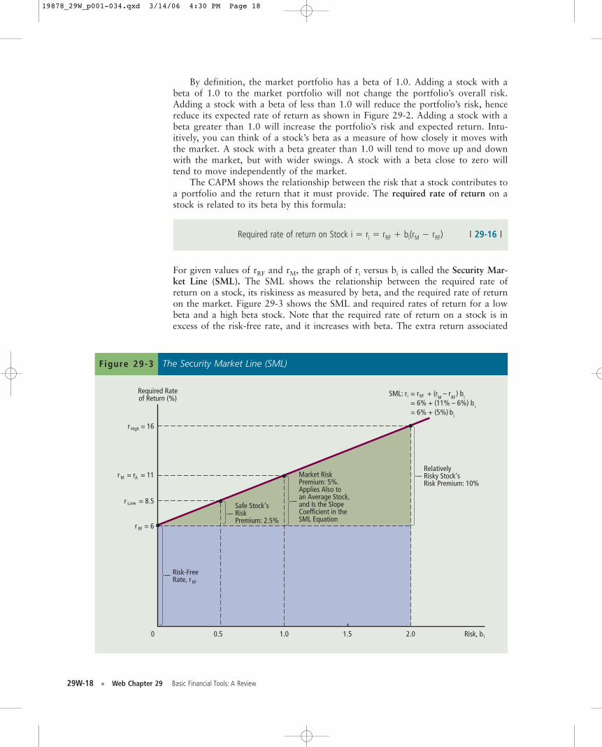
Required rate of return on Stock i � ri � rRF � bi(rM � rRF) | 29-16 |

For given values of rRF and rM, the graph of ri versus bi is called the Security Mar-ket Line (SML). The SML shows the relationship between the required rate ofreturn on a stock, its riskiness as measured by beta, and the required rate of returnon the market. Figure 29-3 shows the SML and required rates of return for a lowbeta and a high beta stock. Note that the required rate of return on a stock is inexcess of the risk-free rate, and it increases with beta. The extra return associated

A

RelativelyRisky Stock’sRisk Premium: 10%

Market RiskPremium: 5%.Applies Also toan Average Stock,and Is the SlopeCoefficient in theSML Equation

Safe Stock’sRiskPremium: 2.5%

Risk-FreeRate, r RF

0 0.5 1.0 1.5 2.0 Risk, b i

r = 16

r = r = 11

r = 8.5

r = 6

Required Rateof Return (%)

High

M

Low

RF

SML: r = r + (r – r ) bii RF M RF

= 6% + (11% – 6%) bi

= 6% + (5%) bi

The Security Market Line (SML)Figure 29-3

19878_29W_p001-034.qxd 3/14/06 4:30 PM Page 18


14Required rates of return are equal to expected rates of return as seen by the marginal investor if markets are efficientand in equilibrium. However, investors may disagree about the investment potential and risk of assets, in which case therequired rate of return may differ from the expected rate of return as seen by an individual investor.

with higher betas is called the risk premium, and the risk premium on a given stockis equal to bi(rM � rRF). The term (rM � rRF), which is called the market risk pre-mium, or RPM, amounts to the extra return an investor requires for bearing themarket’s risk.

The SML graph differs significantly from the CML graph. As Figure 29-2shows, the CML defines the relationship between total risk, as measured by thestandard deviation, and the expected rate of return for portfolios that are combi-nations of the market portfolio and the risk-free asset. It shows the best availableset of portfolios, based on risk and return, available to investors. The SML, on theother hand, shows the relationship between the required rate of return on individ-ual stocks and their market risk as measured by beta.14

The Characteristic Line: Calculating BetasBefore we can use the SML to estimate a stock’s required rate of return, we needto estimate the stock’s beta coefficient. Recall that beta is a measure of how thestock tends to move with the market. Therefore, we can use the historical relation-ship between the stock’s return and the market’s return to calculate beta. First,note the following definitions:

r�J � historical (realized) rate of return on Stock J. (Recall that r̂J and rJ aredefined as Stock J’s expected and required returns, respectively.)

r�M � historical (realized) rate of return on the market.

aJ � vertical axis intercept term for Stock J.

bJ � slope, or beta coefficient, for Stock J.

eJ � random error, reflecting the difference between the actual return onStock J in a given year and the return as predicted by the regressionline. This error arises because of unique conditions that affect Stock Jbut not most other stocks during a particular year.

The points on Figure 29-4 show the historical returns for Stock J plotted against his-torical market returns. The returns themselves are shown in the bottom half of thefigure. The slope of the regression line that best fits these points measures the overallsensitivity of Stock J’s return to the market return, and it is the beta estimate forStock J. The equation for the regression line can be obtained by ordinary leastsquares analysis, using either a calculator with statistical functions or a computerwith a regression software package such as a spreadsheet’s regression function. In his1964 article which first described the CAPM, Sharpe called this regression line thestock’s characteristic line. Thus, a stock’s beta is the slope of its characteristic line.

Figure 29-4 shows that the regression equation for Stock J is as follows:

r�J � �8.9 � 1.6 r�M � eJ | 29-17 |

19878_29W_p001-034.qxd 3/14/06 4:30 PM Page 19


This equation gives the predicted future return on Stock J, given the market’s per-formance in a future year.15 So, if the market’s return happens to be 20 percentnext year, the regression equation predicts that Stock J’s return will be �8.9 �1.6(20) � 23.1%.

We can also use Equation 29-16 to determine the required rate of return onStock J, given the required rate of return on the market and the risk-free rate asshown on the Security Market Line:

rJ � rRF � 1.6(rM � rRF)

15This assumes no change in either the risk-free rate or the market risk premium.

r_

Δ

Realized Returnson Stock J, r (%)

Realized Returnson the Market, r (%)

302010

a = Intercept = – 8.9% r = 8.9% + 7.1% = 16%

= 10% b =RiseRun

= =1610

= 1.6J

MJ

JJ

–10 0

– 20

–10

10

20

30

40

7.1

Year 3

Year 4

Year 5Year 1

= a + b r + e= – 8.9 + 1.6r + e

r J J J M J

M J

_

__

Year 2

_

_

M

J

_

MΔ

r_

Δr_

Δ

Calculating Beta CoefficientsFigure 29-4

Year Stock J ( r–J) Market ( r–M)

1 38.6% 23.8%2 (24.7) (7.2)3 12.3 6.64 8.2 20.55 40.1 30.6

Average r� � 14.9% 14.9%� r– � 26.5% 15.1%

19878_29W_p001-034.qxd 3/14/06 4:30 PM Page 20


| 29-18 |

Thus, if the risk-free rate is 8 percent and the required rate of return on themarket is 13 percent, then the required rate of return on Stock J is 8% � 1.6(13%� 8%) � 16%.

Market versus Diversifiable RiskEquation 29-17 can also be used to show how total, diversifiable, and market riskare related. The total risk for Stock J, �2

J, can be broken down into market riskand diversifiable risk:

Total risk � Variance � Market risk � Diversifiable risk

�2J � b2

J�2M � �2

eJ

Here �2J is Stock J’s variance (or total risk), bJ is the stock’s beta coefficient, �2

M isthe variance of the market, and � 2

eJ is the variance of Stock J’s regression errorterm. If all of the points in Figure 29-4 plotted exactly on the regression line, thenJ would have zero diversifiable risk and the variance of the error term, �2

eJ, wouldbe zero. However, in our example all of the points do not plot exactly on theregression line, and the decomposition of total risk for J is thus

Total risk � 0.2652 � Market risk � Diversifiable risk0.0702 � (1.6)2(0.151)2 � �2

eJ

0.0702 � 0.0584 � �2eJ

Solving for �2eJ gives diversifiable risk of �2

eJ � 0.0118. In standard deviationterms, the market risk is 20.0584 � 24.2%, and the diversifiable risk is20.0118 � 10.9%.

Portfolio BetasThe beta of a portfolio can be calculated as the weighted average of the betas ofthe individual assets in the portfolio. This is in sharp contrast to the difficult calculation required in Equation 29-13 for finding the standard deviation of aportfolio. To illustrate the calculation, suppose an analyst has determined the following information for a four-stock portfolio:

Stock Weight Beta Product(1) (2) (3) (4) � (2) (3)

I 0.40 0.6 0.24J 0.20 1.0 0.20K 0.30 1.3 0.39L 0.10 2.1 0.21

1.00 Portfolio beta: 1.04

The beta is calculated as the sum of the product terms in the table. We could alsocalculate it using this equation:

bp � 0.4(0.6) � 0.2(1.0) � 0.3(1.3) � 0.1(2.1) � 1.04

19878_29W_p001-034.qxd 3/14/06 4:30 PM Page 21


Self-Test Questions

| 29-19 |

Here the first value in each term is the stock’s weight in the portfolio, the secondterm is the stock’s beta, and the weighted average is the portfolio’s beta, bp � 1.04.

Now assume that the risk-free rate is 8 percent, and the required rate ofreturn on the market portfolio is 12 percent. The portfolio’s required return canbe found using Equation 29-16:

rp � 8% � 1.04(12% � 8%) � 12.16%

How are the expected return and standard deviation calculated from a probability distribution?When is the coefficient of variation a useful measure of risk?What is the difference between diversifiable risk and market risk?Explain the following statement: “An asset held as part of a portfolio is generally less risky

than the same asset held in isolation.”What does it mean to say that beta is the theoretically correct measure of a stock’s riskiness?What is the difference between the CML and the SML?How would you calculate a beta?What is optimal about an “optimal portfolio”?

STOCK VALUATION

The techniques used earlier in this chapter to value bonds can also be used, with afew modifications, to value stocks. First, note that the cash flows from stocks thatcompanies provide to investors are dividends rather than coupon payments, andthere is no maturity date on stocks. Moreover, dividend payments are not contrac-tual, and they typically are expected to grow over time, not to remain constant asbond interest payments do. Here is the general equation used to value commonstocks:

Here the Dt terms represent the dividend expected in each year t, and r is thestock’s required rate of return as determined in the preceding section. There is nomaturity date, so the present value must be for all expected dividend paymentsextending out forever.

Equation 29-19 for stocks differs from Equation 29-6 for bonds in that Dtrepresents an expected but uncertain, and nonconstant, dividend rather than afixed, known coupon or principal payment, and also because the summation goesout to infinity. The required rate of return on the stock, r, could either be deter-mined by the CAPM or just estimated subjectively by the investor.

Dividend Growth ModelRather than explicitly projecting dividends forever, under certain assumptions wecan simplify the process. In particular, if our best guess is that the firm’s earningsand dividends will grow at a constant rate g on into the foreseeable future, thenwe can use the dividend growth model. For example, suppose a company has justpaid a dividend of $1.50, and its dividends are projected to grow at a rate of6 percent per year. The expected dividend at the end of the current year will be

Price � PV �D1

(1 � r ) 1�

D2

(1 � r ) 2� p �

Dn

(1 � r ) n� p � a

q

t�1

Dt

(1 � r ) t

19878_29W_p001-034.qxd 3/14/06 4:30 PM Page 22


16See Chapter 5 for the derivation of Equation 29-20.

$1.50(1.06) � $1.59. The dividend expected during the second year willbe $1.50(1.06)2 � $1.6854, and the dividend expected during the t’th year will be$1.50(1.06)t.

We can replace Dt with D0(1 � g)t in Equation 29-19, in which case we havea power series that can be solved to give the following formula:16

| 29-20 |

This equation is called the constant growth model, or the Gordon model afterMyron J. Gordon, who did much to develop and popularize it. In our example,D0 � $1.50 and g � 0.06. If the required rate of return on the stock is 13 percent,then the present value of all expected future dividends will be 1.50(1.06)/(0.13 �0.06) � $22.71, and this is the value of the stock according to the model.

Equation 29-20 also provides an alternative to the CAPM for estimating therequired rate of return on a stock. First, we transform Equation 29-20 to formEquation 29-21:

r̂s � D1/P0 � g | 29-21 |

Here we write the rate of return variable as r̂s rather than r to indicate that it is anexpected as opposed to a required rate of return. The equation indicates that theexpected rate of return on a stock whose dividend is growing at a constant rate, g,is the sum of its expected dividend yield and its constant growth rate. In equilib-rium, this is also the required rate of return.

Both the current price and the most recent dividend can be readily deter-mined, and analysts make and publish growth rate estimates. Thus, given theinput data, we can solve for r̂s. Here is the situation for our illustrative stock:

r̂s � D1/P0 � g � $1.50(1.06)/$22.71 � 0.06 � 0.13 � 13%

In Chapter 11 we discuss the types of firms for which this analysis is appropriate.We also provide other simplified models in the next two sections for use in situa-tions where the assumption of constant growth is not appropriate.

PerpetuitiesA second simplified version of the general stock valuation model as expressed inEquation 29-19 can be used to value perpetuities, which are securities that areexpected to pay a constant amount each period forever. Preferred stock is anexample of a perpetuity. Many preferred stocks have no maturity date, and theypay a constant dividend. In this case g � 0 in Equation 29-20, and the expressionreduces to P � D/r. A share of $3 preferred stock (that is, the stock pays $3 everyyear) with a required rate of return of 9 percent will sell for $3.00/0.09 � $33.33.The perpetuity formula also makes it easy to find the expected yield on a security,

Price now � P̂ 0 �D0 (1 � g)

r � g�

D1

r � g

19878_29W_p001-034.qxd 3/14/06 4:30 PM Page 23


given the dividend and the current price: r̂s � D/P. So, if a share of preferred stockthat pays an annual dividend of $4 per share trades for $65 per share, the stock’syield is $4/$65 � 6.15%.

Nonconstant Growth ModelOften it is inappropriate to assume that a company’s dividends will grow at a con-stant rate forever. Most firms start out small and pay no dividends during theirinitial growth phase. Later, when they are able, they start paying a small dividend,and they then increase this dividend relatively rapidly, as earnings continue togrow. Finally, as the firm begins to mature, its dividend growth rate declines to theoverall growth rate of the company or the industry. Thus, the growth rate is ini-tially zero, then it becomes positive and large, and finally it declines andapproaches a constant rate. In this situation, the dividend growth model given inEquation 29-20 is not appropriate, and an attempt to use it would give inaccurateand misleading results.

The best way to deal with a changing dividend growth rate is to use the non-constant growth model, also called the supermodel growth model. This involvesseveral steps:

• Estimate each dividend during the nonconstant growth period.• Determine the present value of each of the nonconstant growth dividends.• Use the constant growth model to find the discounted value of all of the divi-

dends expected once the nonconstant growth period has ended, which is theexpected stock price at the end of the nonconstant growth period.

• Find the present value of the expected future price.• Sum the PVs of the nonconstant dividends and the PV of the expected future

price to find the value of the stock today.

For example, suppose the required rate of return on a stock is 12 percent. Adividend of $0.25 has just been paid, and you expect the dividend to double eachyear for four years. After Year 4, the firm will reach a steady state and have a div-idend growth rate of 8 percent per year forever. The following time line shows thecash flows:

Growth rate 100% 100% 100% 100% 8% 8%Dividend 0.50 1.00 2.00 4.00 4.32

0 21 3 54

To begin, let’s find the price at the end of the fourth year, at which point we willhave a constant growth stock. Someone buying the stock will receive D5 and thesubsequent dividends, which will presumably grow at a constant rate of 8 percentforever. Equation 29-20 can be used to find P̂4:

| 29-20a |

This means that the constant growth rate model can be used as of Year 4, and thestock price expected in that year is found as follows:

| 29-20b |P̂ 4 �D5

r � g�

4.32

0.12 � 0.08� $108

Price at end of Year 4 � P̂ 4 �D5

r � g

19878_29W_p001-034.qxd 3/14/06 4:30 PM Page 24

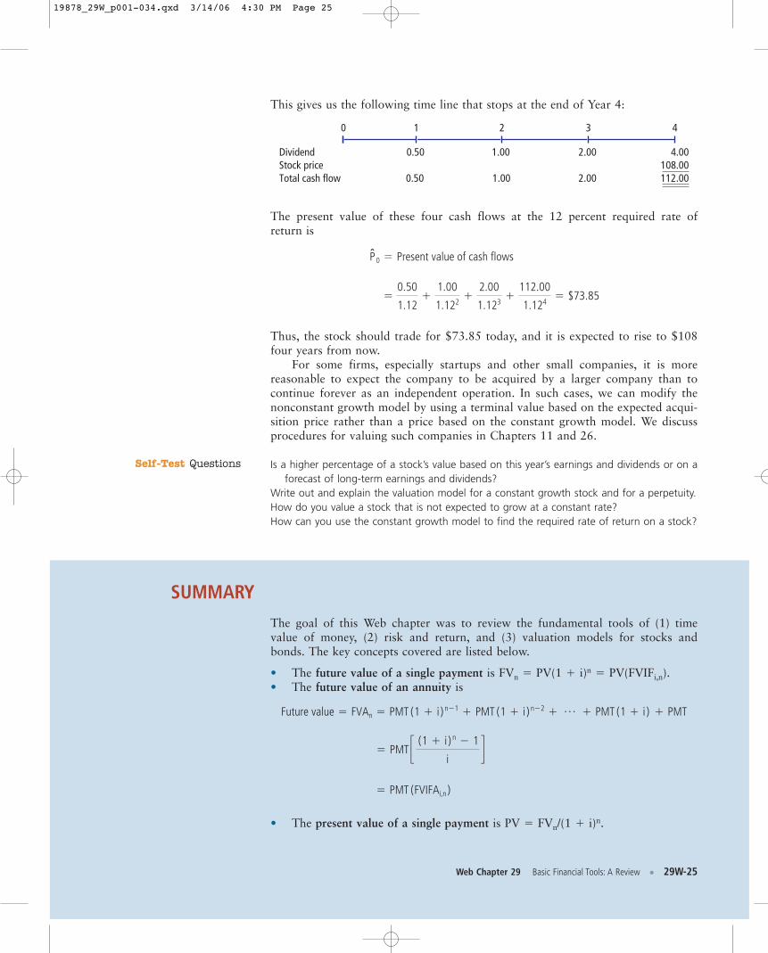
This gives us the following time line that stops at the end of Year 4:

DividendStock priceTotal cash flow 0.50 1.00 2.00

0 1 2 3 4

0.50 1.00 2.00 4.00108.00112.00

Self-Test Questions

The present value of these four cash flows at the 12 percent required rate ofreturn is

Thus, the stock should trade for $73.85 today, and it is expected to rise to $108four years from now.

For some firms, especially startups and other small companies, it is more reasonable to expect the company to be acquired by a larger company than tocontinue forever as an independent operation. In such cases, we can modify thenonconstant growth model by using a terminal value based on the expected acqui-sition price rather than a price based on the constant growth model. We discussprocedures for valuing such companies in Chapters 11 and 26.

Is a higher percentage of a stock’s value based on this year’s earnings and dividends or on aforecast of long-term earnings and dividends?

Write out and explain the valuation model for a constant growth stock and for a perpetuity.How do you value a stock that is not expected to grow at a constant rate?How can you use the constant growth model to find the required rate of return on a stock?

SUMMARY

The goal of this Web chapter was to review the fundamental tools of (1) timevalue of money, (2) risk and return, and (3) valuation models for stocks andbonds. The key concepts covered are listed below.

• The future value of a single payment is FVn � PV(1 � i)n � PV(FVIFi,n).• The future value of an annuity is

• The present value of a single payment is PV � FVn/(1 � i)n.

� PMT (FVIFAi,n )

� PMT c (1 � i ) n � 1

id

Future value � FVAn � PMT (1 � i ) n�1 � PMT (1 � i ) n�2 � p � PMT (1 � i ) � PMT

�0.50

1.12�

1.00

1.122�

2.00

1.123�

112.00

1.124� $73.85

P̂0 � Present value of cash flows


19878_29W_p001-034.qxd 3/14/06 4:30 PM Page 25


• The present value of an annuity is

� PMTC 1 �

1

(1 � i ) n

iS

Present value � PVAn �PMT

(1 � i )�

PMT

(1 � i ) 2�

PMT

(1 � i ) 3� p �

PMT

(1 � i ) n�1�

PMT

(1 � i ) n

� PMT(PVIFAi,n)

• The effective annual rate for m compounding intervals per year at a nominal

rate of inom per year is EAR (or EFF%) � a 1 �iNom

mb

m

� 1.0.

• The effective annual rate for continuous compounding at a nominal rate ofiNom per year is EARcontinuous � eiNom � 1.0.

• If you know the cash flows and the PV (or FV) of a cash flow stream, you candetermine the interest rate using a financial calculator to solve for the interestrate.

• The general valuation equation for a series of cash flows is

• The price of a bond is the present value of its coupon and principal payments:

• The riskiness of an asset’s cash flows can be considered either on a stand-alone basis, with each asset thought of as being held in isolation, or in a port-folio context, where the investment is combined with other assets and its riskis reduced through diversification.

• The relevant risk of an individual asset is its contribution to the riskiness of awell-diversified portfolio, which is the asset’s market risk. This risk is meas-ured by beta. Since market risk cannot be eliminated by diversification,investors must be compensated for bearing it.

• The Security Market Line (SML) equation shows the relationship between asecurity’s risk and its required rate of return. The return required on any secu-rity is equal to the risk-free rate plus the market risk premium times the secu-rity’s beta:

ri � rRF � bi(rM � rRF)

• The Capital Market Line describes the risk/return relationship for optimalportfolios, that is, for portfolios that consist of a mix of the market portfolioand a riskless asset.

• The beta coefficient is measured by the slope of the stock’s characteristic line,which is found by regressing historical returns on the stock versus historicalreturns on the market.

Price of bond �aN

t�1

Coupon

(1 � rd ) t�

Par

(1 � rd ) N

PV �CF1

(1 � i ) 1�

CF2

(1 � i ) 2� p �

CFn

(1 � i ) n�a

n

t�1

CFt

(1 � i ) t

19878_29W_p001-034.qxd 3/14/06 4:30 PM Page 26


• The value of a share of stock is calculated as the present value of the streamof dividends the stock is expected to provide in the future.

• The equation used to find the value of a constant growth stock is

• The equation for r̂s, the expected rate of return on a constant growth stock,can be expressed as follows: r̂s � D1/P0 � g.

• To find the present value of a supernormal growth stock (1) find the dividendsexpected during the supernormal growth period, (2) find the price of the stockat the end of the supernormal growth period, (3) discount the dividends andthe projected price back to the present, and (4) sum these PVs to find thestock’s value, P̂0.

• The value of a perpetuity can be found using the constant growth formulawith g � 0.

QUESTIONS

29-1 Define each of the following terms:a. PV; i or I; FVn; PMT; m; inomb. FVIFi,n; PVIFi,n; FVIFAi,n; PVIFAi,nc. Equivalent annual rate (EAR); nominal (quoted) interest rated. Amortization schedule; principal component versus interest component of a

paymente. Par value; maturity date; coupon payment; coupon interest ratef. Premium bond; discount bondg. Stand-alone risk; risk; probability distributionh. Expected rate of return, r̂ i. Risk premium for Stock i, RPi; market risk premium, RPMj. Capital Asset Pricing Model, CAPMk. Market risk; diversifiable risk; relevant riskl. Beta coefficient, bm.Security Market Line, SMLn. Optimal (or efficient) portfolioo. Capital Market Line, CMLp. Characteristic lineq. Intrinsic value, P̂0; market price, P0r. Required rate of return, rS; expected rate of return, r̂S; actual, or realized, rate

of return, r�S.s. Normal, or constant, growth; supernormal, or nonconstant, growth

29-2 Would you rather have a savings account that pays 5 percent interest compoundedsemiannually, or one that pays 5 percent interest compounded daily? Explain.

29-3 The rate of return you would earn if you bought a bond and held it to its maturitydate is called the bond’s yield to maturity. How is the yield to maturity related tooverall interest rates in the economy? If interest rates in the economy fall after abond has been issued, what will happen to the bond’s yield to maturity and price?Will the size of any changes be affected by the bond’s maturity?

P̂ 0 �D0 (1 � g)

r � g�

D1

r � g

19878_29W_p001-034.qxd 3/14/06 4:30 PM Page 27


29-4 Security X has an expected return of 6 percent, a standard deviation of expectedreturns of 40 percent, a correlation coefficient with the market of �0.20, and abeta coefficient of �0.4. Security Y has an expected return of 13 percent, a stan-dard deviation of returns of 25 percent, a correlation with the market of 0.8, anda beta coefficient of 1.0. Which security is riskier? Why?

29-5 If a stock’s beta were to drop to half of its former level, would its expected returnalso drop by half?

29-6 What is the difference between the SML and the CML?

29-7 Two investors are evaluating GE’s stock for possible purchase. They agree on theexpected value of D1 and also on the expected future dividend growth rate. Fur-ther, they agree on the riskiness of the stock. However, one investor normallyholds stocks for 2 years, while the other normally holds stocks for 10 years. Onthe basis of the type of analysis done in this chapter, should they be willing to paythe same price for GE’s stock? Explain.

PROBLEMS

29-1 Find the future value of the following annuities. The first payment is made at theend of Year 1, so they are ordinary annuities:a. $500 per year for 8 years at 9%.b. $300 per year for 6 years at 4%.c. $500 per year for 6 years at 0%.d. Now rework parts a, b, and c assuming that payments are made at the begin-

ning of each year; that is, they are annuities due.

29-2 Find the present value of the following ordinary annuities:a. $500 per year for 8 years at 9%.b. $300 per year for 6 years at 4%.c. $500 per year for 6 years at 0%.d. Now rework parts a, b, and c assuming that payments are made at the begin-

ning of each year; that is, they are annuities due.

29-3 Find the interest rates, or rates of return, on each of the following:a. You borrow $900 and promise to pay back $972 at the end of 1 year.b. You lend $900 and receive a promise to be paid $972 at the end of 1 year.c. You borrow $65,000 and promise to pay back $310,998 at the end of

15 years.d. You borrow $11,000 and promise to make payments of $2,487.22 per year for

7 years.

29-4 Your grandmother has asked you to evaluate two alternative investments for her.The first is a security that pays $50 at the end of each of the next 3 years, with afinal payment of $1,050 at the end of Year 4. This security costs $900. The secondinvestment involves simply putting the same amount of money in a bank savingsaccount that pays an 8 percent nominal (quoted) interest rate, but with quarterlycompounding. Your grandmother regards the two investments as being equally safeand liquid, so the required effective annual rate of return on the security is thesame as that on the bank deposit. She has asked you to calculate the value of thesecurity to help her decide whether it is a good investment. What is its value rela-tive to the bank deposit?

Future Value of anAnnuity

Present Value of anAnnuity

Effective Rate of Interest

PV and Effective AnnualYield

19878_29W_p001-034.qxd 3/14/06 4:30 PM Page 28


29-5 Assume that your father is now 55 years old, that he plans to retire in 12 years,and that he expects to live for 20 years after he retires, that is, until he is 87. Hewants a fixed retirement income that has the same purchasing power at the time heretires as $60,000 has today (he realizes that the real value of his retirement incomewill decline year by year after he retires, but he wants level payments during retire-ment anyway). His retirement income will begin the day he retires, 12 years fromtoday, and he will receive 20 annual payments. Inflation is expected to be 5 percentper year from today forward. He currently has $100,000 in savings, and he expectsto earn a return on his savings of 8 percent per year, annual compounding. To thenearest dollar, how much must he save during each of the next 12 years (withdeposits being made at the end of each year) to meet his retirement goal?

29-6 Cargill Diggs’s bonds have 15 years remaining to maturity. Interest is paid annually,the bonds have a $1,000 par value, and the coupon interest rate is 9.5 percent. Thebonds sell at a price of $850. What is their yield to maturity?

29-7 The Peabody Company has two bond issues outstanding. Both pay $110 annualinterest plus $1,000 at maturity. Bond H has a maturity of 14 years and Bond K amaturity of 2 years.a. What is the value of each of these bonds if the going rate of interest is

(1) 5 percent, (2) 8 percent, and (3) 12 percent? Assume that two more interestpayments will be made on Bond K and 14 more on Bond H.

b. Why does the longer-term (14-year) bond fluctuate more when interest rateschange than does the shorter-term bond (2-year)?

29-8 Suppose Integon Inc. sold an issue of bonds with a 10-year maturity, a $1,000 parvalue, a 9 percent coupon rate, and semiannual interest payments.a. Two years after the bonds were issued, the going rate of interest on bonds such

as these fell to 7 percent. At what price would the bonds sell?b. Suppose that, 2 years after the initial offering, the going interest rate had risen

to 11 percent. At what price would the bonds sell?c. Suppose that the conditions in part a existed—that is, interest rates fell to

7 percent 2 years after the issue date. Suppose further that the interest rateremained at 7 percent for the next 8 years. What would happen to the price ofthe Integon bonds over time? (Hint: How much should one of these bonds sellfor just before maturity?)

29-9 A bond trader purchased each of the following bonds at a yield to maturity of9 percent. Immediately after she purchased the bonds, interest rates fell to 8 per-cent. To show the price sensitivity of each bond to changes in interest rates, fill inthe blanks in the following table:

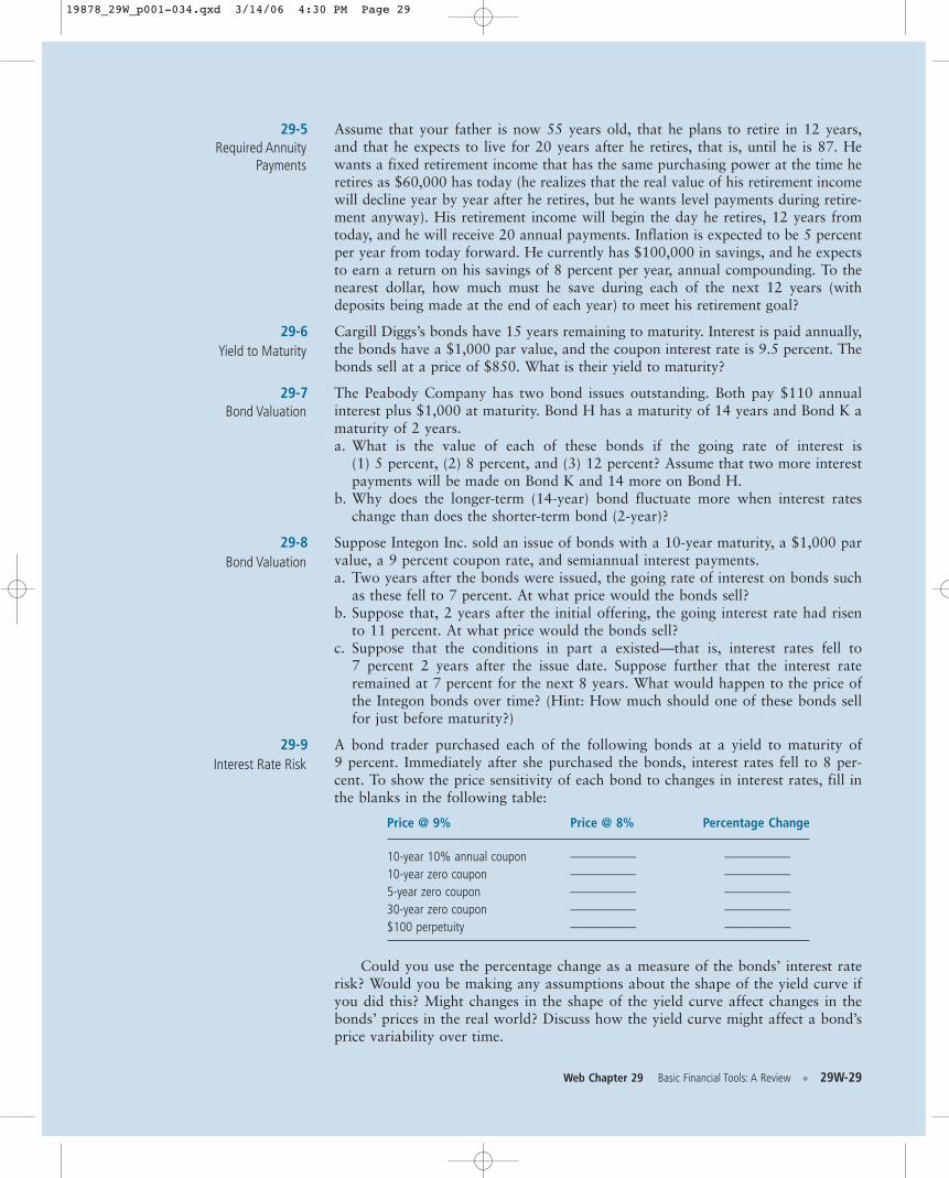
Price @ 9% Price @ 8% Percentage Change

10-year 10% annual coupon ————— —————10-year zero coupon ————— —————5-year zero coupon ————— —————30-year zero coupon ————— —————$100 perpetuity ————— —————

Could you use the percentage change as a measure of the bonds’ interest raterisk? Would you be making any assumptions about the shape of the yield curve ifyou did this? Might changes in the shape of the yield curve affect changes in thebonds’ prices in the real world? Discuss how the yield curve might affect a bond’sprice variability over time.

Required AnnuityPayments

Yield to Maturity

Bond Valuation

Bond Valuation

Interest Rate Risk

19878_29W_p001-034.qxd 3/14/06 4:30 PM Page 29


29-10 An investor has two bonds in his portfolio. Each bond matures in 3 years, has aface value of $1,000, and has a yield to maturity of 11.1 percent. Bond A pays anannual coupon of 13 percent. Bond Z is a zero coupon bond. Assuming the yield tomaturity of each bond remains at 11.1 percent over the next 4 years, what will bethe price of each of the bonds at the following time periods? Fill in the followingtable:

t Price of Bond A Price of Bond Z

0 ————— —————1 ————— —————2 ————— —————3 ————— —————

29-11 A stock’s expected return has the following distribution:

Rate of ReturnDemand for the Probability of This If This DemandCompany’s Products Demand Occurring Occurs

Weak 0.2 (40%)Below average 0.2 (10)Average 0.1 8Above average 0.3 20Strong 0.2 50

Calculate the stock’s expected return, standard deviation, and coefficient of variation.

29-12 An individual has $60,000 invested in a stock that has a beta of 1.3 and $15,000invested in a stock with a beta of 0.6. If these are the only two investments in herportfolio, what is her portfolio’s beta?

29-13 Suppose rRF � 9%, rM � 14%, and rA � 20%.a. Calculate Stock A’s beta.b. If Stock A’s beta changed to 1.5, how would the required rate of return change?

29-14 Suppose rRF � 6%, rM � 11%, and bi � 1.3.a. What is ri, the required rate of return on Stock i?b. Now suppose rRF (1) increases to 7 percent or (2) decreases to 5 percent. The

slope of the SML remains constant. How would this affect rM and ri?c. Now assume that rRF remains at 6 percent but rM (1) increases to 13 percent or

(2) falls to 10 percent. The slope of the SML does not remain constant. Howwould these changes affect ri?

29-15 You have a $3 million portfolio consisting of a $150,000 investment in each of 20different stocks. The portfolio has a beta of 1.2. You are considering selling$150,000 worth of one stock that has a beta equal to 0.8 and using the proceedsto purchase a stock that has a beta equal to 1.4. What will be the new beta ofyour portfolio following this transaction?

Bond Valuation

Expected Return

Portfolio Beta

Required Rate of Return

Required Rate of Return

Portfolio Beta

19878_29W_p001-034.qxd 3/14/06 4:30 PM Page 30


29-16 You are given the following set of data:Characteristic Line and

SML

SML and CMLComparison

Constant GrowthValuation

Constant GrowthValuation

a. Use a calculator with a linear regression function (or a spreadsheet) to deter-mine Stock ABC’s beta coefficient, or else plot these data points on a scatterdiagram, draw in the regression line, and then estimate the value of the betacoefficient “by eye.”

b. Determine the arithmetic average rates of return for Stock ABC and the NYSEover the period given. Calculate the standard deviations of returns for bothStock ABC and the NYSE.

c. Assuming (1) that the situation during Years 1 to 7 is expected to hold true inthe future (that is, r̂ABC � r�ABC; r�M � r̂M; and both �ABC and bABC in the futurewill equal their past values), and (2) that Stock ABC is in equilibrium (that is, itplots on the SML), what is the implied risk-free rate?

d. Plot the Security Market Line.e. Suppose you hold a large, well-diversified portfolio and are considering adding

to the portfolio either Stock ABC or another stock, Stock Y, that has the samebeta as Stock ABC but a higher standard deviation of returns. Stocks ABC andY have the same expected returns; that is r̂ABC � r̂Y � 10.6%. Which stockshould you choose?

29-17 The beta coefficient of an asset can be expressed as a function of the asset’s correla-tion with the market, its standard deviation, and the market’s standard deviation:

a. Substitute this expression for beta into the Security Market Line (SML), Equa-tion 29-16. This results in an alternative form of the SML.

b. Compare your answer to part a with the Capital Market Line (CML), Equation29-14. What similarities are observed? What conclusions can be drawn?

29-18 Axxon Inc. is expected to pay a $0.75 per share dividend at the end of theyear (i.e., D1 � $0.75). The dividend is expected to grow at a constant rate of7 percent a year. The required rate of return on the stock, rs, is 15 percent. Whatis the value of a share of the company’s stock?

29-19 Pic-A-Shoe’s stock currently sells for $25. The stock just paid a dividend of $1.25;that is, D0 � $1.25. The dividend is expected to grow at a constant rate of 8 percent

bi ��i,M �i

�M

HISTORICAL RATES OF RETURN

Year NYSE Stock ABC

1 (26.5%) (14.5%)2 37.2 23.53 23.8 17.04 (7.2) 2.55 6.6 7.66 20.5 19.97 30.6 18.2

19878_29W_p001-034.qxd 3/14/06 4:30 PM Page 31


a year. What stock price is expected 1 year from now? What is the required rate ofreturn?

29-20 Escrow Oil’s petroleum reserves are being depleted, so its sales revenues arefalling. Also, its reserves are becoming increasingly deep each year, so the costs ofbringing oil to the surface are rising. As a result, the company’s earnings and divi-dends are declining at a constant rate of 5 percent per year. If D0 � $6 and rS �15%, what is the value of Escrow Oil’s stock?

29-21 Assume that an average firm in your company’s industry is expected to grow at aconstant rate of 7 percent and has a dividend yield of 6 percent. Your company isof average risk, but it has just successfully completed some R&D work that leadsyou to expect that its earnings and dividends will grow at a rate of 50 percent [D1 � D0(1 � g) � D0(1.50)] this year, and 25 percent the following year, afterwhich growth should match the 7 percent industry average rate. The last dividendpaid (D0) was $2.00. What is the value per share of your firm’s stock today?(Hint: Use Equation 29-21 to find the required rate of return.)

29-22 Jonesboro Corporation issued preferred stock with a stated dividend of 9 percentof par. Preferred stock of this type currently yields 7 percent, and the par value is$100. Assume dividends are paid annually.a. What is the value of Jonesboro Corporation’s preferred stock?b. Suppose interest rate levels rise to the point where preferred stock yields 12 per-

cent. Now what would be the value of Jonesboro’s preferred stock?

SPREADSHEET PROBLEM

29-23 Start with the partial model in the file IFM9 Ch29 P23 Build a Model.xls fromthe ThomsonNOW Web site. Set up an amortization schedule for a $30,000 loanto be repaid in equal installments at the end of each of the next 20 years at aninterest rate of 10 percent.a. What is the annual payment?b. Set up an amortization schedule for a $60,000 loan to be repaid in 20 equal

annual installments at an interest rate of 10 percent. What is the annual payment?

c. Set up an amortization schedule for a $60,000 loan to be repaid in 20 equalannual installments at an interest rate of 20 percent. What is the annual payment?

CYBERPROBLEM

Please go to the ThomsonNOW Web site to access any Cyberproblems.

Declining Growth StockValuation

Supernormal GrowthStock Valuation

Preferred Stock Valuation

Build a Model: LoanAmortization

19878_29W_p001-034.qxd 3/14/06 4:30 PM Page 32


Susan Greene is a financial planner. Her job is tosuggest and implement investment and savings plansfor clients, some of whom are of modest means andsome of whom are quite wealthy. Last month a Fortune 500 firm contracted with Susan’s firm toprovide financial planning services to all 150 of itsmiddle-level managers over a 3-month period.Susan’s plan is first to conduct an hour-long seminarto provide some general information about invest-ments and their risks, and then to arrange individualmeetings for follow-up. She has asked you to helpher with the seminar by working out some examplesto illustrate savings and investment plans, and toprepare some information about the risks andrewards of investments in common stock. She partic-ularly wants you to explain how risk and return arerelated. Please answer the following questions andprepare the following illustrations for her.

a. Draw time lines (1) for a $100 lump sum due atthe end of Year 2 and (2) for a 3-year $100annuity. Explain how each investment of $100grows to its future value after 3 years if theinterest rate is 10 percent.

b. What is the present value of the $100 lump sumdue at the end of 2 years and the 3-year, $100annuity in part a? How much would you needto invest in an account that earns 10 percent inorder to fund this annuity?

c. If inflation is 3 percent per year, then an annualsalary of $60,000 today will rise to about$145,000 in 30 years. One of Susan’s clientswants to maintain a purchasing power of$60,000 in today’s dollars, at least for the firstyear of retirement, so she is planning to draw$145,000 a year at year-end after retirement.How much must she save monthly to retire in30 years and draw an annual pension of$145,000 for 20 years after retirement? Assumea 10 percent per year return on investments.

d. Susan has also asked you to prepare some infor-mation about various investments that might beused to meet these retirement goals. To do thisyou will need to discuss not only how bondsand stocks are priced but also the concept of thetrade-off between risk and return. To begin,describe the key features of a bond and show

how its value is determined. Find the value of a10-year, $1,000 par value bond with a 10 per-cent annual coupon and a required rate ofreturn of 10 percent.

e. (1) What would be the value of the bonddescribed in part d if, just after it had beenissued, the expected inflation rate rose by 3percentage points, causing investors torequire a 13 percent return?

(2) What would happen to the bond’s value ifinflation fell, causing rd to decline to 7 per-cent?

(3) What would happen to the value of the 10-year bond over time if the required rateof return remained at 13 percent? If itremained at 7 percent?

f. As an alternative to bond investments, Susanwants you to present some data on stock invest-ments. The following table has the returns thatshould occur under various states of the econ-omy for a variety of assets. Some of the outputvariables have been calculated, but blanks areshown for others.(1) Calculate the expected return, standard

deviation, and CV for HT and the T-bills.(2) How do HT’s return, standard deviation,

and CV compare with those of the otherassets, and what are the implications ofthese comparisons?

g. Suppose you created a 2-stock portfolio by invest-ing $50,000 in HT and $50,000 in Collections.(1) Calculate the expected return (rP), the stan-

dard deviation (�p), and the coefficient ofvariation (CVp) for this portfolio.

(2) How does the riskiness of this portfoliocompare to the riskiness of the individualstocks if held in isolation?

h. Explain what happens to the risk and expectedreturn on a portfolio constructed from randomlypicked stocks if we start with a 1-stock portfolioand add more and more stocks.

i. How are risk and return related under theCAPM? Specifically, how is beta calculated andhow are required rates of return determined?Use the SML to calculate required rates ofreturn for the three stocks in part f. How do

19878_29W_p001-034.qxd 3/14/06 4:30 PM Page 33

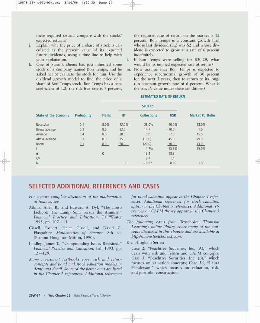
ESTIMATED RATE OF RETURN

STOCKS

State of the Economy Probability T-Bills HT Collections USR Market Portfolio

Recession 0.1 8.0% (22.0%) 28.0% 10.0% (13.0%)Below average 0.2 8.0 (2.0) 14.7 (10.0) 1.0Average 0.4 8.0 20.0 0.0 7.0 15.0Above average 0.2 8.0 35.0 (10.0) 45.0 29.0Boom 0.1 8.0 50.0 (20.0) 30.0 43.0r̂ 1.7% 13.8% 15.0%� 0 13.4 18.8CV 7.7 1.4b 1.30 �0.87 0.89 1.00

For a more complete discussion of the mathematicsof finance, see

Atkins, Allen B., and Edward A. Dyl, “The LottoJackpot: The Lump Sum versus the Annuity,”Financial Practice and Education, Fall/Winter1995, pp. 107–111.

Cissell, Robert, Helen Cissell, and David C.Flaspohler, Mathematics of Finance, 8th ed.(Boston: Houghton Mifflin, 1990).

Lindley, James T., “Compounding Issues Revisited,”Financial Practice and Education, Fall 1993, pp.127–129.

Many investment textbooks cover risk and returnconcepts and bond and stock valuation models indepth and detail. Some of the better ones are listedin the Chapter 2 references. Additional references

for bond valuation appear in the Chapter 4 refer-ences. Additional references for stock valuationappear in the Chapter 5 references. Additional ref-erences on CAPM theory appear in the Chapter 3references.

The following cases from Textchoice, ThomsonLearning’s online library, cover many of the con-cepts discussed in this chapter and are available athttp://www.textchoice2.com.

Klein-Brigham Series:

Case 2, “Peachtree Securities, Inc. (A),” whichdeals with risk and return and CAPM concepts;Case 3, “Peachtree Securities, Inc. (B),” whichfocuses on valuation concepts; Case 56, “LauraHenderson,” which focuses on valuation, risk,and portfolio construction.

SELECTED ADDITIONAL REFERENCES AND CASES


these required returns compare with the stocks’expected returns?

j. Explain why the price of a share of stock is cal-culated as the present value of its expectedfuture dividends, using a time line to help withyour explanation.

k. One of Susan’s clients has just inherited somestock of a company named Bon Temps, and heasked her to evaluate the stock for him. Use thedividend growth model to find the price of ashare of Bon Temps stock. Bon Temps has a betacoefficient of 1.2, the risk-free rate is 7 percent,

the required rate of return on the market is 12percent. Bon Temps is a constant growth firmwhose last dividend (D0) was $2 and whose div-idend is expected to grow at a rate of 6 percentindefinitely.

l. If Bon Temps were selling for $30.29, whatwould be its implied expected rate of return?

m. Now assume that Bon Temps is expected toexperience supernormal growth of 30 percentfor the next 3 years, then to return to its long-run constant growth rate of 6 percent. What isthe stock’s value under these conditions?

19878_29W_p001-034.qxd 3/14/06 4:30 PM Page 34

Documents

19878 29W p001-034 - Cengage · TIME VALUE OF MONEY Time value concepts, ... For a more detailed review of time value of money concepts, see Web Chapter 28 ... 19878_29W_p001-034.qxd