601.433/633 Introduction to Algorithms Lecturer: Michael DinitzTopic: Max-Flow Min-Cut Date: 10/28/21

18.1 Introduction

We are given a directed graph G = (V,E) with positive capacities on the edges, c : E → R+. Thissetup is sometimes called a flow network. We will slightly abuse notation and let c(u, v) = 0 if(u, v) 6∈ E, since this will let us simplify the notation a bit. We will also usually have two specialvertices, s and t. For reasons that will become clear, we usually call s the source and t the sink.We will be concerned today with two different but very related concepts: flows and cuts. We’ll talka bit about algorithms, but most of the real algorithmic analysis will happen next lecture.

18.2 Flows

Flows are a pretty intuitive concept: a flow from s to t is basically a way of sending “stuff” from sto t. Famous examples include sewer systems, railroad networks, and many others. More formally,an (s, t)-flow is a function f : E → R≥0 such that∑

u:(u,v)∈E

f(u, v) =∑

u:(v,u)∈E

f(v, u) (18.2.1)

for all vertices v ∈ V \ {s, t}. We might sometimes abuse notation and say that f(u, v) = 0 if(u, v) 6∈ E. These equalities are known as flow conservation: at every vertex other than the sourceand the destination, the total flow in is equal to the total flow out.

The value of the flow, which is sometimes denoted by |f |, is the “total amount of stuff” that we’resending from the source to the sink. Since the flow conservation constraints imply that flow in =flow out at all intermediate nodes, the total amount of stuff that we’re sending is equal to the totalamount of stuff leaving the source, which is equal to the total amount of stuff entering the sink. So

|f | =∑

u:(s,u)∈E

f(s, u)−∑

u:(u,s)∈E

f(u, s) =∑

u:(u,t)∈E

f(u, t)−∑

u:(t,u)∈E

f(t, u)

Of course, our flows have to live within the given capacities. So we also have capacity constraintson our flow:

f(u, v) ≤ c(u, v) (18.2.2)

for all (u, v) ∈ E. A flow which satisfies the capacity constraints is sometimes called a feasible flow.If f(u, v) = c(u, v) then we say that f saturates edge e, and if f(e) = 0 we say that f avoids edgee. Let’s see an example:

1

Algorithms Lecture ��: Maximum Flows and Minimum Cuts [Fa’��]

amount of material that can be transported from s to t; the minimum cut problem asks for theminimum damage needed to separate s from t.

��.� Flows

An (s , t )-flow (or just a flow if the source and target are clear from context) is a functionf : E! R�0 that satisfies the following conservation constraint at every vertex v except possiblys and t: X

u

f (u�v) =X

w

f (v�w).

In English, the total flow into v is equal to the total flow out of v. To keep the notation simple,we define f (u�v) = 0 if there is no edge u�v in the graph. The value of the flow f , denoted | f |,is the total net flow out of the source vertex s:

| f | :=X

w

f (s�w)�X

u

f (u�s).

It’s not hard to prove that | f | is also equal to the total net flow into the target vertex t, asfollows. To simplify notation, let @ f (v) denote the total net flow out of any vertex v:

@ f (v) :=X

u

f (u�v)�X

w

f (v�w).

The conservation constraint implies that @ f (v) = 0 or every vertex v except s and t, soX

v

@ f (v) = @ f (s) + @ f (t).

On the other hand, any flow that leaves one vertex must enter another vertex, so we must havePv @ f (v) = 0. It follows immediately that | f |= @ f (s) = �@ f (t).Now suppose we have another function c : E! R�0 that assigns a non-negative capacity c(e)

to each edge e. We say that a flow f is feasible (with respect to c) if f (e) c(e) for every edge e.Most of the time we will consider only flows that are feasible with respect to some fixed capacityfunction c. We say that a flow f saturates edge e if f (e) = c(e), and avoids edge e if f (e) = 0.The maximum flow problem is to compute a feasible (s, t)-flow in a given directed graph, witha given capacity function, whose value is as large as possible.

s t

10/20

0/10

10/10

0/5

10/10

5/15

5/10

5/20

0/15

An (s, t)-flow with value 10. Each edge is labeled with its flow/capacity.

��.� Cuts

An (s , t )-cut (or just cut if the source and target are clear from context) is a partition of thevertices into disjoint subsets S and T—meaning S [ T = V and S \ T = ?—where s 2 S andt 2 T .

�

We are going to be talking about algorithms for computing the maximum flow, i.e., a flow f whichmaximizes |f |.

18.3 Cuts

An (s, t)-cut is a partition of the vertices into two sets (S, S̄) (recall that S̄ = V \ S) wheres ∈ S, t ∈ S̄. Much of the times we will simply talk about the cut S, since S̄ is implied by S. Thecapacity of a cut (S, S̄) is the total capacity of the edges from S to S̄:

cap(S, S̄) =∑

(u,v)∈E:u∈S,v∈S̄

c(u, v) =∑u∈S

∑v∈S̄

c(u, v). (18.3.3)

Note that the capacity does not take into account the capacity of edges from S̄ to S. There areother, essentially equivalent definitions of cuts in terms of edge sets, but we’re going to mostly stickwith this definition.

Let’s see another quick example:

Algorithms Lecture ��: Maximum Flows and Minimum Cuts [Fa’��]

If we have a capacity function c : E! R�0, the capacity of a cut is the sum of the capacitiesof the edges that start in S and end in T :

kS, Tk :=Xv2S

Xw2T

c(v�w).

(Again, if v�w is not an edge in the graph, we assume c(v�w) = 0.) Notice that the definition isasymmetric; edges that start in T and end in S are unimportant. The minimum cut problem isto compute an (s, t)-cut whose capacity is as large as possible.

s t

20

10

10

5

10

15

10

20

15

An (s, t)-cut with capacity 15. Each edge is labeled with its capacity.

Intuitively, the minimum cut is the cheapest way to disrupt all flow from s to t. Indeed, itis not hard to show that the value of any feasible (s , t )-flow is at most the capacity of any(s , t )-cut. Choose your favorite flow f and your favorite cut (S, T ), and then follow the bouncinginequalities:

| f |=X

w

f (s�w)�X

u

f (u�s) by definition

=Xv2S

✓Xw

f (v�w)�X

u

f (u�v)

◆by the conservation constraint

=Xv2S

ÇXw2T

f (v�w)�Xu2T

f (u�v)

åremoving duplicate edges

Xv2S

Xw2T

f (v�w) since f (u�v)� 0

Xv2S

Xw2T

c(v�w) since f (u�v) c(v�w)

= kS, Tk by definition

Our derivation actually implies the following stronger observation: | f | = kS, Tk if and only iff saturates every edge from S to T and avoids every edge from T to S. Moreover, if we havea flow f and a cut (S, T ) that satisfies this equality condition, f must be a maximum flow, and(S, T ) must be a minimum cut.

��.� The Maxflow Mincut Theorem

Surprisingly, for any weighted directed graph, there is always a flow f and a cut (S, T ) thatsatisfy the equality condition. This is the famous max-flow min-cut theorem, first proved by LesterFord (of shortest path fame) and Delbert Ferguson in ���� and independently by Peter Elias,Amiel Feinstein, and and Claude Shannon (of information theory fame) in ����.

�

We will mostly be concerned with the minimum cut problem, where we try to compute the cut ofminimum capacity.

2

18.4 Max-Flow Min-Cut

It’s not hard to see that the minimum cut is at least the maximum flow. Slightly more generally, it’snot hard to see that the value of any (s, t)-flow is at most the capacity of any (s, t) cut. Intuitively,this is because if we have a cut of some capacity α, then since any flow has to “cross” the cut, it isonly possible to send α flow. Let’s prove this a bit more formally.

Lemma 18.4.1 Let f be a feasible (s, t)-flow, and let (S, S̄) be an (s, t)-cut. Then |f | ≤ cap(S, S̄).

Proof:

|f | =∑v

f(s, v)−∑v

f(v, s) (definition)

=∑u∈S

(∑v

f(u, v)−∑v

f(v, u)

)(flow conservation constraints)

=∑u∈S

∑v∈S̄

f(u, v)−∑v∈S̄

f(v, u)

(remove terms which cancel)

≤∑u∈S

∑v∈S̄

f(u, v) (flow is nonnegative)

≤∑u∈S

∑v∈S̄

c(u, v) (flow is feasible)

= cap(S, S̄)

This proof actually implies something a little stronger, which we’ll use later:

Corollary 18.4.2 Let f be a feasible (s, t)-flow and let (S, S̄) be an (s, t)-cut. If f saturates everyedge from S to S̄ and avoids every edge from S̄ to S, then |f | = cap(S, S̄) and f is a maximumflow and (S, S̄) is a minimum cut.

What is not as easy to see is that this upper bound is actually tight: the maximum flow has valueequal to the capacity of the minimum cut. This is known as the Max-Flow Min-Cut theorem:

Theorem 18.4.3 In any flow network with source s and sink t, the value of the maximum flow isequal to the capacity of the minimum cut.

We will spent the rest of the lecture proving this theorem. Note that Lemma 18.4.1 implies thatthe value of the maximum flow is at most the capacity of the minimum cut.

While it is possible to prove this theorem structurally, we will give a proof which naturally leads toan algorithm (albeit not a very fast algorithm). This approach is due to Ford and Fulkerson, andthe resulting algorithm is known as the Ford-Fulkerson algorithm. First, though, we’re going to doa simple transformation which will make the notation a little easier. We want to assume that thereare no cycles of length 2 in the graph, i.e., that if (u, v) ∈ E then (v, u) 6∈ E. This is definitely nottrue in general, but it’s not hard to see that we can make it true without losing anything. To dothis, we will actually insert a new vertex. If both (u, v) and (v, u) are edges, we will add a new

3

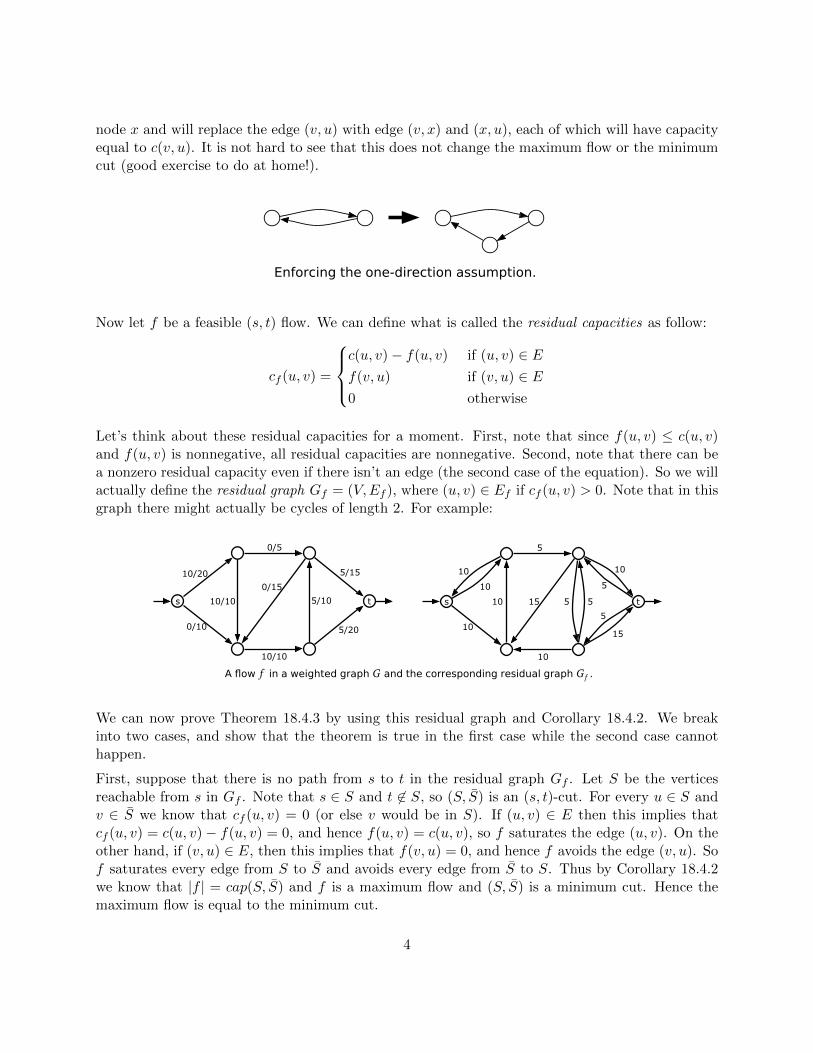
node x and will replace the edge (v, u) with edge (v, x) and (x, u), each of which will have capacityequal to c(v, u). It is not hard to see that this does not change the maximum flow or the minimumcut (good exercise to do at home!).

Algorithms Lecture ��: Maximum Flows and Minimum Cuts [Fa’��]

The Maxflow Mincut Theorem. In any flow network with source s and target t, the value of themaximum (s, t)-flow is equal to the capacity of the minimum (s, t)-cut.

Ford and Fulkerson proved this theorem as follows. Fix a graph G, vertices s and t, and acapacity function c : E! R�0. The proof will be easier if we assume that the capacity functionis reduced: For any vertices u and v, either c(u�v) = 0 or c(v�u) = 0, or equivalently, if anedge appears in G, then its reversal does not. This assumption is easy to enforce. Whenever anedge u�v and its reversal v�u are both the graph, replace the edge u�v with a path u�x�v oflength two, where x is a new vertex and c(u�x) = c(x�v) = c(u�v). The modified graph hasthe same maximum flow value and minimum cut capacity as the original graph.

Enforcing the one-direction assumption.

Let f be a feasible flow. We define a new capacity function c f : V ⇥ V ! R, called theresidual capacity, as follows:

c f (u�v) =

8><>:

c(u�v)� f (u�v) if u�v 2 E

f (v�u) if v�u 2 E

0 otherwise.

Since f � 0 and f c, the residual capacities are always non-negative. It is possible to havec f (u�v) > 0 even if u�v is not an edge in the original graph G. Thus, we define the residualgraph Gf = (V, Ef ), where Ef is the set of edges whose residual capacity is positive. Notice thatthe residual capacities are not necessarily reduced; it is quite possible to have both c f (u�v)> 0and c f (v�u)> 0.

s t

10/20

0/10

10/10

0/5

10/10

5/15

5/10

5/20

0/15s t

10

10

5

10

515 5

10

5

15

5

10

10

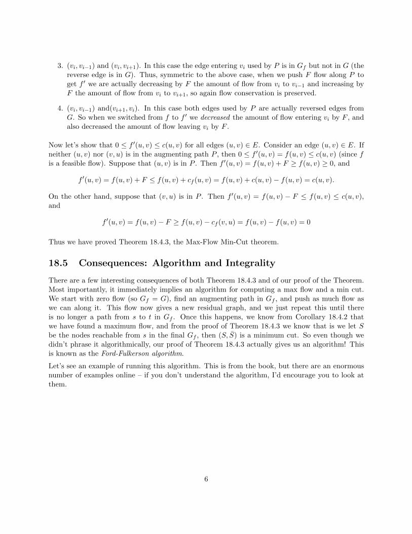
A flow f in a weighted graph G and the corresponding residual graph Gf .

Suppose there is no path from the source s to the target t in the residual graph Gf . Let Sbe the set of vertices that are reachable from s in Gf , and let T = V \ S. The partition (S, T ) isclearly an (s, t)-cut. For every vertex u 2 S and v 2 T , we have

c f (u�v) = (c(u�v)� f (u�v)) + f (v�u) = 0,

which implies that c(u�v)� f (u�v) = 0 and f (v�u) = 0. In other words, our flow f saturatesevery edge from S to T and avoids every edge from T to S. It follows that | f |= kS, Tk. Moreover,f is a maximum flow and (S, T ) is a minimum cut.

On the other hand, suppose there is a path s = v0�v1� · · ·�vr = t in Gf . We refer tov0�v1� · · ·�vr as an augmenting path. Let F =mini c f (vi�vi+1) denote the maximum amount

�

Now let f be a feasible (s, t) flow. We can define what is called the residual capacities as follow:

cf (u, v) =

c(u, v)− f(u, v) if (u, v) ∈ Ef(v, u) if (v, u) ∈ E0 otherwise

Let’s think about these residual capacities for a moment. First, note that since f(u, v) ≤ c(u, v)and f(u, v) is nonnegative, all residual capacities are nonnegative. Second, note that there can bea nonzero residual capacity even if there isn’t an edge (the second case of the equation). So we willactually define the residual graph Gf = (V,Ef ), where (u, v) ∈ Ef if cf (u, v) > 0. Note that in thisgraph there might actually be cycles of length 2. For example:

Algorithms Lecture ��: Maximum Flows and Minimum Cuts [Fa’��]

The Maxflow Mincut Theorem. In any flow network with source s and target t, the value of themaximum (s, t)-flow is equal to the capacity of the minimum (s, t)-cut.

Ford and Fulkerson proved this theorem as follows. Fix a graph G, vertices s and t, and acapacity function c : E! R�0. The proof will be easier if we assume that the capacity functionis reduced: For any vertices u and v, either c(u�v) = 0 or c(v�u) = 0, or equivalently, if anedge appears in G, then its reversal does not. This assumption is easy to enforce. Whenever anedge u�v and its reversal v�u are both the graph, replace the edge u�v with a path u�x�v oflength two, where x is a new vertex and c(u�x) = c(x�v) = c(u�v). The modified graph hasthe same maximum flow value and minimum cut capacity as the original graph.

Enforcing the one-direction assumption.

Let f be a feasible flow. We define a new capacity function c f : V ⇥ V ! R, called theresidual capacity, as follows:

c f (u�v) =

8><>:

c(u�v)� f (u�v) if u�v 2 E

f (v�u) if v�u 2 E

0 otherwise.

Since f � 0 and f c, the residual capacities are always non-negative. It is possible to havec f (u�v) > 0 even if u�v is not an edge in the original graph G. Thus, we define the residualgraph Gf = (V, Ef ), where Ef is the set of edges whose residual capacity is positive. Notice thatthe residual capacities are not necessarily reduced; it is quite possible to have both c f (u�v)> 0and c f (v�u)> 0.

s t

10/20

0/10

10/10

0/5

10/10

5/15

5/10

5/20

0/15s t

10

10

5

10

515 5

10

5

15

5

10

10

A flow f in a weighted graph G and the corresponding residual graph Gf .

Suppose there is no path from the source s to the target t in the residual graph Gf . Let Sbe the set of vertices that are reachable from s in Gf , and let T = V \ S. The partition (S, T ) isclearly an (s, t)-cut. For every vertex u 2 S and v 2 T , we have

c f (u�v) = (c(u�v)� f (u�v)) + f (v�u) = 0,

which implies that c(u�v)� f (u�v) = 0 and f (v�u) = 0. In other words, our flow f saturatesevery edge from S to T and avoids every edge from T to S. It follows that | f |= kS, Tk. Moreover,f is a maximum flow and (S, T ) is a minimum cut.

On the other hand, suppose there is a path s = v0�v1� · · ·�vr = t in Gf . We refer tov0�v1� · · ·�vr as an augmenting path. Let F =mini c f (vi�vi+1) denote the maximum amount

�

We can now prove Theorem 18.4.3 by using this residual graph and Corollary 18.4.2. We breakinto two cases, and show that the theorem is true in the first case while the second case cannothappen.

First, suppose that there is no path from s to t in the residual graph Gf . Let S be the verticesreachable from s in Gf . Note that s ∈ S and t 6∈ S, so (S, S̄) is an (s, t)-cut. For every u ∈ S andv ∈ S̄ we know that cf (u, v) = 0 (or else v would be in S). If (u, v) ∈ E then this implies thatcf (u, v) = c(u, v)− f(u, v) = 0, and hence f(u, v) = c(u, v), so f saturates the edge (u, v). On theother hand, if (v, u) ∈ E, then this implies that f(v, u) = 0, and hence f avoids the edge (v, u). Sof saturates every edge from S to S̄ and avoids every edge from S̄ to S. Thus by Corollary 18.4.2we know that |f | = cap(S, S̄) and f is a maximum flow and (S, S̄) is a minimum cut. Hence themaximum flow is equal to the minimum cut.

4

Now suppose that there is a path from s to t in Gf . We will try to derive a contradiction to showthat this cannot happen. Let this path be s = v0, v1, v2, . . . , vr = t, and call this path P . Withoutloss of generality, we may assume that there are no cycles on this path (if there are cycles thenwe can just find a shorter path without cycles). Such a path (from s to t in the residual graph) iscalled an augmenting path. Let F = minr−1

i=0 cf (vi, vi+1). We are going to claim that we can “push”F more flow from s to t, so f is not actually a maximum flow. This will prove Theorem 18.4.3.

Consider the new flow f ′ : E → R≥0 defined as follows:

f ′(u, v) =

f(u, v) + F if (u, v) in P

f(u, v)− F if (v, u) in P

f(u, v) otherwise

Let’s see a quick example:Algorithms Lecture ��: Maximum Flows and Minimum Cuts [Fa’��]

s t

10

10

5

10

515 5

10

5

15

5

10

10

s t

10/20

5/10

5/10

5/5

10/10

5/15

0/10

10/20

0/15

An augmenting path in Gf with value F = 5 and the augmented flow f 0.

of flow that we can push through the augmenting path in Gf . We define a new flow functionf 0 : E! R as follows:

f 0(u�v) =

8><>:

f (u�v) + F if u�v is in the augmenting pathf (u�v)� F if v�u is in the augmenting pathf (u�v) otherwise

To prove that the flow f 0 is feasible with respect to the original capacities c, we need to verifythat f 0 � 0 and f 0 c. Consider an edge u�v in G. If u�v is in the augmenting path, thenf 0(u�v)> f (u�v)� 0 and

f 0(u�v) = f (u�v) + F by definition of f 0

f (u�v) + c f (u�v) by definition of F

= f (u�v) + c(u�v)� f (u�v) by definition of c f

= c(u�v) Duh.

On the other hand, if the reversal v�u is in the augmenting path, then f 0(u�v) < f (u�v) c(u�v), which implies that

f 0(u�v) = f (u�v)� F by definition of f 0

� f (u�v)� c f (v�u) by definition of F

= f (u�v)� f (u�v) by definition of c f

= 0 Duh.

Finally, we observe that (without loss of generality) only the first edge in the augmenting pathleaves s, so | f 0|= | f |+ F > 0. In other words, f is not a maximum flow.

This completes the proof!

��.� Ford and Fulkerson’s augmenting-path algorithm

Ford and Fulkerson’s proof of the Maxflow-Mincut Theorem translates immediately to analgorithm to compute maximum flows: Starting with the zero flow, repeatedly augment the flowalong any path from s to t in the residual graph, until there is no such path.

This algorithm has an important but straightforward corollary:

Integrality Theorem. If all capacities in a flow network are integers, then there is a maximumflow such that the flow through every edge is an integer.

�

Note that P leaves the source s once and never comes back (since there are no cycles in P ). Thus|f ′| = |f | + F > |f |. So if we can show that f ′ is a feasible flow under the original capacities, wewill have a contradiction with our assumption that f is a maximum (s, t)-flow.

Let’s first show that flow conservation holds in f ′ at all nodes other than s and t. Consider somenode v. If P does not enter or leave v then f ′(u, v) = f(u, v) and f ′(v, u) = f(v, u) for all u,so since flow conservation held under f , it also holds under f ′. Now consider some vi ∈ P withvi 6= s, t. Intuitively, since we pushed F new flow through P , whatever change happened to theincoming flow to vi also happened to the outgoing flow. To prove this more formally, note that theonly edges with changed flow are the edge between vi and vi−1, and the edge between vi and vi+1.So we just need to prove that the change in flow in these edges balances out. We’ll break into fourcases depending on the directions of the underlying edges.

1. (vi−1, vi) and (vi, vi+1). In this case the edges used by P are edges in G (not just in Gf ).Thus when using f ′ instead of f the total flow into vi goes up by F , but the total flow out ofvi also goes up by F , and hence flow conservation is maintained.

2. (vi−1, vi) and (vi+1, vi). In this case the edge leaving vi used by P is in Gf but not in G (thereverse edge is in G). Thus f ′(vi−1, vi) = f(vi−1, vi) + F , and f ′(vi+1, vi) = f(vi+1, vi) − F .So the total flow entering and leaving vi remains the same, so flow conservation is preserved.

5

3. (vi, vi−1) and (vi, vi+1). In this case the edge entering vi used by P is in Gf but not in G (thereverse edge is in G). Thus, symmetric to the above case, when we push F flow along P toget f ′ we are actually decreasing by F the amount of flow from vi to vi−1 and increasing byF the amount of flow from vi to vi+1, so again flow conservation is preserved.

4. (vi, vi−1) and(vi+1, vi). In this case both edges used by P are actually reversed edges fromG. So when we switched from f to f ′ we decreased the amount of flow entering vi by F , andalso decreased the amount of flow leaving vi by F .

Now let’s show that 0 ≤ f ′(u, v) ≤ c(u, v) for all edges (u, v) ∈ E. Consider an edge (u, v) ∈ E. Ifneither (u, v) nor (v, u) is in the augmenting path P , then 0 ≤ f ′(u, v) = f(u, v) ≤ c(u, v) (since fis a feasible flow). Suppose that (u, v) is in P . Then f ′(u, v) = f(u, v) + F ≥ f(u, v) ≥ 0, and

f ′(u, v) = f(u, v) + F ≤ f(u, v) + cf (u, v) = f(u, v) + c(u, v)− f(u, v) = c(u, v).

On the other hand, suppose that (v, u) is in P . Then f ′(u, v) = f(u, v) − F ≤ f(u, v) ≤ c(u, v),and

f ′(u, v) = f(u, v)− F ≥ f(u, v)− cf (v, u) = f(u, v)− f(u, v) = 0

Thus we have proved Theorem 18.4.3, the Max-Flow Min-Cut theorem.

18.5 Consequences: Algorithm and Integrality

There are a few interesting consequences of both Theorem 18.4.3 and of our proof of the Theorem.Most importantly, it immediately implies an algorithm for computing a max flow and a min cut.We start with zero flow (so Gf = G), find an augmenting path in Gf , and push as much flow aswe can along it. This flow now gives a new residual graph, and we just repeat this until thereis no longer a path from s to t in Gf . Once this happens, we know from Corollary 18.4.2 thatwe have found a maximum flow, and from the proof of Theorem 18.4.3 we know that is we let Sbe the nodes reachable from s in the final Gf , then (S, S̄) is a minimum cut. So even though wedidn’t phrase it algorithmically, our proof of Theorem 18.4.3 actually gives us an algorithm! Thisis known as the Ford-Fulkerson algorithm.

Let’s see an example of running this algorithm. This is from the book, but there are an enormousnumber of examples online – if you don’t understand the algorithm, I’d encourage you to look atthem.

6

We’ll spend most of next lecture actually analyzing the running time of this algorithm (and ofsome variants), but before we do that, I want to point out a structural feature of this algorithm

7

which actually gives a very weak running time bound. Suppose that all of the capacities in ournetwork are integers. Then it is easy to see by induction that everything stays integral throughoutthe running of the algorithm. So we actually have the following integrality theorem:

Theorem 18.5.1 If all capacities in a flow network are integers, then there is a maximum flowsuch that the flow through every edge is an integer.

Moreover, in this case we also have an upper bound on the running time. If the maximum flowpossible is F and all capacities are integers, then in every iteration we push at least 1 unit of flow.So there are at most F iterations. Each iteration simply requires finding a path from s to t in theresidual graph, which takes only O(m+n) time by using DFS or BFS. Thus we get the following:

Theorem 18.5.2 If all capacities in a flow network are integers and the maximum flow value isF , then the running time of Ford-Fulkerson is at most O(F (m+ n)).

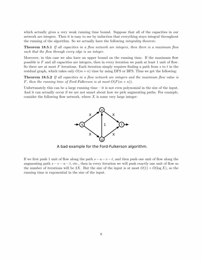
Unfortunately this can be a large running time – it is not even polynomial in the size of the input.And it can actually occur if we are not smart about how we pick augmenting paths. For example,consider the following flow network, where X is some very large integer:

Algorithms Lecture ��: Maximum Flows and Minimum Cuts [Fa’��]

Proof: We argue by induction that after each iteration of the augmenting path algorithm, allflow values and residual capacities are integers. Before the first iteration, residual capacities arethe original capacities, which are integral by definition. In each later iteration, the inductionhypothesis implies that the capacity of the augmenting path is an integer, so augmenting changesthe flow on each edge, and therefore the residual capacity of each edge, by an integer.

In particular, the algorithm increases the overall value of the flow by a positive integer, whichimplies that the augmenting path algorithm halts and returns a maximum flow. É

If every edge capacity is an integer, the algorithm halts after | f ⇤| iterations, where f ⇤ isthe actual maximum flow. In each iteration, we can build the residual graph Gf and perform awhatever-first-search to find an augmenting path in O(E) time. Thus, for networks with integercapacities, the Ford-Fulkerson algorithm runs in O(E| f ⇤|) time in the worst case.

The following example shows that this running time analysis is essentially tight. Considerthe �-node network illustrated below, where X is some large integer. The maximum flow in thisnetwork is clearly 2X . However, Ford-Fulkerson might alternate between pushing � unit of flowalong the augmenting path s�u�v�t and then pushing � unit of flow along the augmenting paths�v�u�t, leading to a running time of ⇥(X ) = ⌦(| f ⇤|).

ts

X

X

1

X

Xu

v

A bad example for the Ford-Fulkerson algorithm.

Ford and Fulkerson’s algorithm works quite well in many practical situations, or in settingswhere the maximum flow value | f ⇤| is small, but without further constraints on the augmentingpaths, this is not an efficient algorithm in general. The example network above can be describedusing only O(log X ) bits; thus, the running time of Ford-Fulkerson is actually exponential in theinput size.

��.� Irrational Capacities

If we multiply all the capacities by the same (positive) constant, the maximum flow increaseseverywhere by the same constant factor. It follows that if all the edge capacities are rational,then the Ford-Fulkerson algorithm eventually halts, although still in exponential time.

However, if we allow irrational capacities, the algorithm can actually loop forever, alwaysfinding smaller and smaller augmenting paths! Worse yet, this infinite sequence of augmentationsmay not even converge to the maximum flow, or even to a significant fraction of the maximumflow! Perhaps the simplest example of this effect was discovered by Uri Zwick.

Consider the six-node network shown on the next page. Six of the nine edges have somelarge integer capacity X , two have capacity 1, and one has capacity � = (

p5�1)/2⇡ 0.618034,

chosen so that 1�� = �2. To prove that the Ford-Fulkerson algorithm can get stuck, we canwatch the residual capacities of the three horizontal edges as the algorithm progresses. (Theresidual capacities of the other six edges will always be at least X � 3.)

Suppose the Ford-Fulkerson algorithm starts by choosing the central augmenting path, shownin the large figure on the next page. The three horizontal edges, in order from left to right, nowhave residual capacities 1, 0, and �. Suppose inductively that the horizontal residual capacitiesare �k�1, 0, �k for some non-negative integer k.

�

If we first push 1 unit of flow along the path s−u− v− t, and then push one unit of flow along theaugmenting path s− v− u− t, etc., then in every iteration we will push exactly one unit of flow sothe number of iterations will be 2X. But the size of the input is at most O(1) + O(logX), so therunning time is exponential in the size of the input.

8