1596 JOURNAL OF ATMOSPHERIC AND …radarmet.atmos.colostate.edu/pdf/CHILLDescip.pdf1596 JOURNAL OF ATMOSPHERIC AND OCEANIC TECHNOLOGY VOLUME 17 q 2000 American Meteorological Society

1596 VOLUME 17J O U R N A L O F A T M O S P H E R I C A N D O C E A N I C T E C H N O L O G Y

q 2000 American Meteorological Society

A Description of the CSU–CHILL National Radar Facility

DAVID BRUNKOW

Department of Atmospheric Science, Colorado State University, Fort Collins, Colorado

V. N. BRINGI

Department of Electrical Engineering, Colorado State University, Fort Collins, Colorado

PATRICK C. KENNEDY AND STEVEN A. RUTLEDGE


V. CHANDRASEKAR

Department of Electrical Engineering, Colorado State University, Fort Collins, Colorado

E. A. MUELLER AND ROBERT K. BOWIE


(Manuscript received 19 May 1999, in final form 29 November 1999)

ABSTRACT

The subject of this paper is the Colorado State University–University of Chicago–Illinois State Water Survey(CSU–CHILL) National Radar Facility’s S-band polarimetric research radar. Key features of this system includepolarization agility (provided by the dual-transmitter, dual-receiver design), a recently updated signal processor,and a low (234 dB, two way) integrated cross-polar ratio (ICPR2) antenna system. After reviewing the technicaldescription of the radar, the authors present a new differential reflectivity (ZDR) calibration technique and dataexamples collected in different polarization modes.

Although the CSU–CHILL radar is transportable, it can also be operated in a dual-Doppler configuration withthe CSU–Pawnee radar, an 11-cm Doppler radar system situated 48 km north of the CSU–CHILL Greeley fieldsite. Used together, these radars provide three-dimensional kinematic and hydrometeor information in precipi-tating cloud systems.

1. Introduction

Meteorological radars have proven to be of great util-ity in remotely sensing the structure and evolution ofclouds and precipitation. Within the last decade, sig-nificant advances have been made in the application ofpolarization diversity technology to meteorological ra-dar (Bringi and Hendry 1990; Doviak and Zrnic 1993).

The foundation of microwave radar remote sensingis the acquisition of useful target information basedupon the amplitude and phase characteristics of the sig-nal received due to backscattering. Polarimetric radarsystems typically transmit and receive signals with two

Corresponding author address: David Brunkow, Department ofAtmospheric Science, Colorado State University, Fort Collins, CO80523.E-mail: [email protected]

orthogonal polarizations. By analyzing the polarizationcomponents of the return signal, information regardingthe mean shape, orientation, and thermodynamic phaseof the particles in the pulse volume can be obtained(McCormick and Hendry 1975; Jameson 1985; Jamesonand Johnson 1990).

In concept, virtually all dual-polarization measure-ments involve the quantification of some change in thereceived signal characteristics based on the transmittedpolarization state. Often the characteristics of these po-larization-dependent signals make their precision mea-surement very difficult (i.e., small magnitudes, largevariances, etc.). To minimize system-induced errors,dual-polarization radars must be carefully designed. Inparticular, the main radiation lobe of the antenna shouldilluminate each sample volume with radiation of highpolarization purity (McCormick 1981). Receivers forboth the copolar and cross-polar return signal compo-nents are necessary to measure the target’s backscat-

DECEMBER 2000 1597B R U N K O W E T A L .

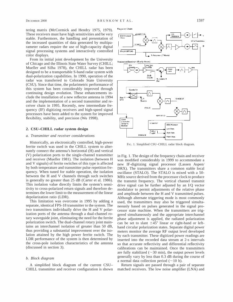
FIG. 1. Simplified CSU–CHILL radar block diagram.

tering matrix (McCormick and Hendry 1975, 1979).These receivers must have high sensitivities and be verystable. Furthermore, the handling and presentation ofthe increased quantities of data generated by multipa-rameter radars require the use of high-capacity digitalsignal processing systems and interactively controlledcolor displays.

From its initial joint development by the Universityof Chicago and the Illinois State Water Survey (CHILL;Mueller and Silha 1978), the CHILL radar has beendesigned to be a transportable S-band radar system withdual-polarization capabilities. In 1990, operation of theradar was transferred to Colorado State University(CSU). Since that time, the polarimetric performance ofthis system has been considerably improved throughcontinuing design evolution. These enhancements in-clude the installation of a new reflector antenna in 1994and the implementation of a second transmitter and re-ceiver chain in 1995. Recently, new intermediate fre-quency (IF) digitizing receivers and high-speed signalprocessors have been added to the system for improvedflexibility, stability, and precision (Wu 1998).

2. CSU–CHILL radar system design

a. Transmitter and receiver considerations

Historically, an electronically controlled, high-powerferrite switch was used in the CHILL system to alter-nately connect the antenna’s horizontal (H) and vertical(V) polarization ports to the single-channel transmitterand receiver (Mueller 1981). The isolation (between Hand V signals) of ferrite switches of this type is affectedby both temperature and transmitter pulse repetition fre-quency. When tuned for stable operation, the isolationbetween the H and V channels through such switchesis generally no greater than 25 dB (Carter et al. 1986).This isolation value directly limits the system’s sensi-tivity to cross-polarized return signals and therefore de-termines the lower limit to the measurement of the lineardepolarization ratio (LDR).

This limitation was overcome in 1995 by adding aseparate, identical FPS-18 transmitter to the system. Thetwo transmitters individually drive the H and V polar-ization ports of the antenna through a dual-channel ro-tary waveguide joint, eliminating the need for the ferritepolarization switch. The dual-channel rotary joint main-tains an interchannel isolation of greater than 50 dB,thus providing a substantial improvement over the iso-lation attained by the high power ferrite switch. TheLDR performance of the system is then determined bythe cross-pole isolation characteristics of the antenna(discussed in section 3).

b. Block diagram

A simplified block diagram of the current CSU–CHILL transmitter and receiver configuration is shown

in Fig. 1. The design of the frequency chain and receiverwas modified considerably in 1999 to accommodate anew IF-digitizing signal processor (Lassen Aspen/DRX). The transmitters share a common stable localoscillator (STALO). The STALO is mixed with a 50-MHz source derived from the processor clock to producethe transmit frequency. The vertical channel transmitdrive signal can be further adjusted by an I/Q vectormodulator to permit adjustments of the relative phaseand amplitude between the H and V transmitted pulses.Although alternate triggering mode is most commonlyused, the transmitters may also be triggered simulta-neously based on pulses generated in the signal pro-cessor state machine. When the transmitters are trig-gered simultaneously and the appropriate interchannelphase adjustment is applied, the radiated polarizationcan be set to slant 6458 linear or right-hand or left-hand circular polarization states. Separate digital powermeters monitor the average RF output level developedby each transmitter. These digitized power readings areinserted into the recorded data stream at 2-s intervalsso that accurate reflectivity and differential reflectivitycalibrations can be maintained. Once the transmittersare fully stabilized (;30 min), the output power levelsgenerally vary by less than 0.3 dB during the course ofa normal data collection period (;10 h).

Return signals are passed through a pair of separatematched receivers. The low noise amplifier (LNA) and


FIG. 2. Gain difference as a function of input power.

first mixers for both receivers are mounted on the samealuminum plate. The temperature of the plate is held ata constant value (208C) by a thermostatically controlledPeltier effect cooler. The minimization of temperaturevariations between the ‘‘front end’’ components of thetwo receiver channels reduces the tendency for differ-ential drifts to develop in the calibration characteristicsof the two receivers.

A solid state transfer switch located after each LNApermits the H and V received signals returning from theantenna to be connected to either receiver channel. Priorto 1999, the transfer switch was used to route all thecopolar signals to one receiver and all the cross-polarsignals to the other receiver. In the alternating VH op-erational mode, this switch was toggled just before eachpulse was transmitted. The reasoning was that using asingle receiver to develop the copolar radar measurables,such as ZH, the differential reflectivity (ZDR), the dif-ferential phase (f DP), and the copolar correlation co-efficient (rHV) (Doviak and Zrnic 1993) would reduceerrors due to calibration differences and drift in the tworeceivers. The stability and linearity of the current dig-ital receivers are believed to be of sufficiently high qual-ity that the transfer switch, while still in the circuit, isnot currently in use. Figure 2 indicates the power dif-ference as measured by the two receivers when bothreceivers were driven by a test signal that was split andfed into both waveguides simultaneously. The resultsindicate less than 0.1-dB difference in gain between theH and the V receivers over a wide dynamic range.

From the transfer switch, the received signals passthrough image rejection filters and are down convertedto a 50-MHz IF by mixing with the STALO frequency.A second conversion to the 10-MHz IF is performed bymixing with the 40-MHz reference clock from the pro-cessor. The IF signal is converted by 12-bit digitizersrunning at a 40-MHz rate. Programmable FIR filterchips then apply quadrature detection followed by low-pass filtering to produce in-phase (I) and quadrature (Q)voltage numbers. Each processor performs these func-tions in a pair of receiver channels separated in sensi-

tivity by 25 dB. When all samples are complete for agiven integration period, the set that offers the mostsensitivity without excessive saturation will be selectedfor processing. To facilitate this channel selection pro-cess, each range gate has a counter to keep track of thenumber of saturated samples encountered during eachintegration cycle. The bank of counters is available tothe digital signal processors (DSPs), where the actualdecision on which receiver channel to use is made. Newdirectional couplers have been added between the trans-mitters and the circulators, which provide a high qualitysample of each transmitted pulse that is downconvertedto 10 MHz, just as it is done in the receiver. The transmitsample is then fed to a third input channel on eachprocessor, where the pulse is digitized at a 40-MHz rate.The processor uses these samples to calculate the av-erage amplitude and phase of each pulse and optionallyuses these results to correct the received signals fromthat pulse for slight variations in phase and magnitude.Although the phase stability of the new system has notyet been measured, these corrections are expected toproduce mean phase estimation accuracies of better than0.18. A series of Analog Devices SHARC DSP chipsperforms this correction, applies clutter filtering, anddoes covariance processing. A third-party SHARC-based processor board is used to calculate the meteo-rological moments. The data stream is passed to a work-station for archiving and further distribution. TheSHARC digital signal processing chips offer consider-able computational capability with a software devel-opment environment, which allows most of the pro-gramming to be done in the C language.

In the alternate VH triggering mode, both the copolarH received from H transmitted (HH) and V receivedfrom V transmitted (VV) as well as the cross-polar Vreceived from H transmitted (VH) and HV (cross-poleH received from V transmitted) signals are available.These returns allow both columns of the backscatteringmatrix to be measured and calculation of the covariancematrix elements, albeit not all measured at zero time lag(three real power terms and three complex correlations;Doviak and Zrnic 1993). A list of all data fields availablefrom the CSU–CHILL radar is provided in Table 1. Anoverall summary of the CSU–CHILL radar’s currentperformance characteristics is shown in Table 2.

The enhanced computational speed of the new pro-cessor will allow the testing of a faster scanning modefor the acquisition of the polarization parameters. Theantenna scan rate is a function of the rate at whichindependent samples can be acquired and the numberof independent samples required for a given accuracy.The polarization parameters such as ZDR and f DP requirehigh accuracy, which implies a large number of inde-pendent samples and traditionally slower scan rates(Sachidananda and Zrnic 1985). By trimming the trans-mitted pulse width and the receiver gate size, the in-dividual pulse volume (range gate) depth can be reducedto 45 m. Range averaging of groups of five successive


TABLE 1. Data fields available from the CSU–CHILL system.

Power (dBm)Normalized coherent power (NCP; ratio)Mean radial velocity (m s21)Velocity spectral width (m s21)Differential reflectivity (ZDR; dB)Linear depolarization ratio (LDRH; LDRV, dB)Differential propagation phase (fDP; deg)|HV correlation at lag zero| (rHV)Time series: (digitized individual in phase and quadrature voltages)

Raw floating-point covariance availability matrixAvailable in VH mode

Time lag

Lag 0Lag 1Lag 2

Copol

|HH|2, |VV|2

HHVV*, VVHH*

HHHH*

Cross-pol

|HV|2, |VH|2

HVVH*

Co*cross

HHVH*, VVHV*

Available in VHS (hybrid basis mode)Time lag

Lag 0Lag 1Lag 2

Copol

|H|2, |V|2, HV*

HH*, VV*

HH*, VV*

45-m gates yields a final range resolution of 225 m whileincreasing the number of independent signal samples byapproximately a factor of 4 in comparison to that ob-tained with a conventional 1-ms sample (150-m rangegate). This rapid acquisition of independent samples al-lows the antenna scan rate to be doubled during polar-imetric data collection while maintaining the same ac-curacy in the meteorological fields. Azimuth rates of128 s21 are typical of this mode.

c. Data display and recording

The data stream from the real-time computation sys-tem is made available to multiple local workstations viaan Ethernet network. Conventional plan views and ver-tical cross sections can be produced and controlled in-dependently by each workstation. Position tracks canalso be overlaid on the radar images to aid in projectcoordination when working with research aircraft orground-based chase vehicles. One workstation also hasthe task of archiving the data on disk files. These filesare subsequently moved to 8-mm data cartridges forlong-term storage.

3. Evaluation of antenna performance

Because of the distributed nature of hydrometeor tar-gets, antenna performance is of prime importance. Ac-curate dual-polarization measurements require, ideally,matched copolar beam patterns at both polarizations,low copolar and cross-polar sidelobe levels, and highpolarization purity throughout the main radiation lobe(Bringi and Hendry 1990). When strong reflectivity gra-dients exist across the main beam and close-in sidelobes,even slight copolar pattern mismatches can potentiallycause significant errors in ZDR (e.g., Herzegh and Car-

bone 1984; Pointin et al. 1988). To reduce such errorsit is generally best to reduce the close-in sidelobe levelsas much as possible. The cross-polarization pattern fora linearly polarized antenna has maxima that lie in 458/1358 planes between the principal axes of the antenna.These maxima consist of a set of four pencil-beam lobeson the 458/1358 planes (Wood 1980). The new antennainstalled on the CSU–CHILL radar in 1994 has maxi-mum cross-polar lobe levels of 233 dB in the 458/1358planes. The worst-case, close-in copolar sidelobes areless than 227 dB in any plane. The measured 1358 planeantenna patterns are shown in Fig. 3.

The (two-way) integrated cross-polar ratio (ICPR2)is a figure of merit of dual-polarized antennas and isclosely related to the LDR limit of the system (Ussailisand Metcalf 1983). The ICPR2 in the 458/1358 planeswas computed from measured patterns (Fig. 3) and wasfound to be 234 dB. The ICPR2 is defined by

f f sinu duE co cx

ICPR 5 10 log , (1)2 10

2f sinu du E co

where f co and f cx are the measured copolar and cross-polar patterns, respectively. The CSU–CHILL systemroutinely measures (lower bound) LDR values in the233 to 234 dB range in spatially homogenous precip-itation when the signal-to-noise ratio (SNR) is high (co-polar SNR . ;35 dB). For example, Fig. 4 shows ascatter plot of LDRVH for a number of range profilesmeasured during the Fort Collins, Colorado, flood eventon 28 July 1997 (Petersen et al. 1999). Data points withcopolar SNR . 35 dB are shown. Note that the lower-bound LDRVH from the data is very near 234 dB 6 1


TABLE 2. CSU–CHILL system characteristics.

AntennaShapeDiameterFeed typeGainBeamwidth (3dB)Maximum sidelobeInterchannel isolationICPR (two way)

Parabolic8.5 mScalar43 dB (includes waveguide loss)1.18227 dB (in any f plane)245 dB (limited by orothomode transducer)234 dB

TransmittersWavelengthPeak powerFinal PA typePRT rangePulse widthAvailable polarizations

11.01 cm800 kWVA-87B/C (Klystron)800–2500 ms0.3–1.0 msHorizontal, vertical, slant 458/1358, right/left circular

Receivers/digital signal processingNoise figureNoise power (SNR 5 1)Dynamic rangeBandwidthOutput range resolution

;3.4 dB;2114.0 dBm;96 dB750 kHz typ. with programmable filter45-m minimum, adjustable upward in 15-m intervals

Maximum range gates Estimated to be .3000

FIG. 4. Scatterplot of LDR (dB) vs range (km) for low elevationangle CSU–CHILL PPI data collected during heavy rain (28–29 Aug1997). Only LDR values associated with signal-to-noise ratios (SNRs)above 35 dB are included.

FIG. 3. Copolar and cross-polar power plots. Antenna patterns arein the plane containing the feed horn support structure (f 5 1358).Cross-polar power scale is raised 20 dB above the copolar powerscale. (After Mueller et al. 1995.)

dB. (The subscript ‘‘VH,’’ as in LDRVH, implies a cal-culation based on horizontal transmit and vertical re-ceive.)

When the spatial distribution of scatterers is inhom-ogenous, it is well known that the resultant cross-beamgradients across the main beam and close-in sidelobescan induce antenna pattern related errors, which biasthe estimates of ZDR, LDR, rHV, and, to a lesser extent,f DP (Pointin et al. 1988; Hubbert et al. 1998). In orderto estimate the magnitude of the errors in ZDR and LDRdue to gradients across the beam, specified cross-beamprofiles of ZHH, ZDR, and LDR are input to a simulationprogram. Error estimates are then developed by con-volving these input profiles with the antenna patternsmeasured by the manufacturer in any specified plane

(08, 458, 1358, or 908). For ZDR the simplest approxi-mation is

2Z f dRE HH HH

sm Z 5 10 log , (2)DR 10

2Z f dR E VV VV

where ZHH and ZVV are the input cross-beam reflectivityprofiles and f HH and f VV are the (one way) measuredpower patterns in the azimuthal (f 5 08) plane. The


superscript ‘‘sm’’ on ZDR (and other variables) refers tothe simulated values. Note that all reflectivity units usedhere are expressed in mm6 m23. This equation assumesno cross-polar error due to the antenna and is sufficientlyaccurate for evaluation of errors in ZDR due to mis-

matches in the main and sidelobes (Herzegh and Car-bone 1984).

The approximation for LDR is (Blanchard and New-ton 1985)

(Z f f 1 Z f f 1 Z f f ) dRE VH VV HH HH HH HV VV VV VH

sm LDR 5 10 log , (3)10

2Z f dR E HH HH

where ZHV is the cross-polar reflectivity profile and f HV

5 f VH is the cross-polar power pattern. An additionalterm involving ZVH( f VH)2 is neglected in the numeratorof (3) since it is small in comparison to the other giventerms. Because the f 5 458/1358 plane (containing thefeed support struts and waveguide runs) is the worst forcross-polar errors, the measured antenna patterns for thisplane as well as in the f 5 08 plane are chosen for theestimation of LDR errors.

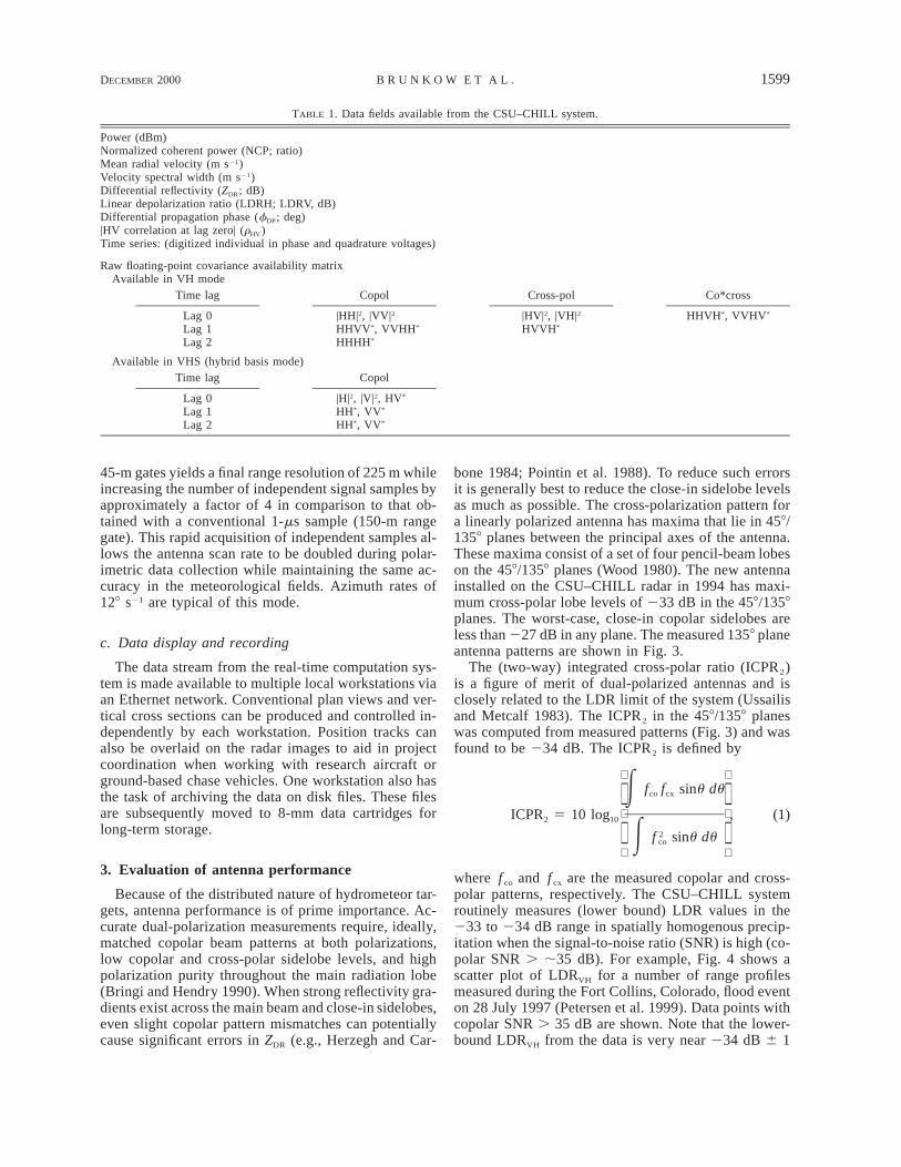
The input ZH profile was chosen to be representativeof a hail shaft embedded in rain at a range of 30 km(Fig. 5a). The reflectivity gradient on the flanks of thehailshaft was chosen to be 30 dB km21. The ZDR profilesharply increases from 0 to 5 dB in the rain and thensharply decreases to ;0 dB in the center of the hailregion (Fig. 5b; see also Aydin et al. 1986). The sim-ulated ZDR profile based on the sampling characteristicsof the measured antenna pattern is quite accurate (Fig.5b) within the constant reflectivity region (20–25 km).As expected, ZDR errors can be noted near the maximumgradient region, but these are well known and have beendocumented (Pointin et al. 1988). Errors are also evidentin the simulated LDR profile in the maximum ZH gra-dient regions (Fig. 5c). In the high ZH gradient region,the LDR error is primarily due to the ZHH f HH f HV andthe ZVV f VV f VH terms in (3). The LDR errors are slightlyworse for cross-beam distances ,19 km or .26 km inthe f 5 458 plane, where the antenna feed supportstructure raises the cross-polar sidelobe levels. Withinthe uniform reflectivity region (20–25 km), the LDRerrors are negligible, since the error is dominated by theZVH f VV f HH term in (3), and the input LDR exceeds theantenna cross-polar error levels, that is, the result is dueto smoothing of the input LDR profile by the copolarpattern. These results show that even with antenna per-formance approaching the theoretically expected max-imum levels for a prime-focus-fed reflector design, radardata may be corrupted in high-reflectivity gradient re-gions. Experience has shown that the CSU–CHILL LDRand ZDR values should be viewed with caution in areaswhere the cross-beam spatial reflectivity gradient ex-ceeds 20–25 dB km21. Antenna performance better than

that illustrated here would result only from the use ofoffset-fed reflector designs, which eliminate beamblockage by the feed support structure.

4. The ZDR calibration techniques

Rainfall estimators based on the combination of Zand ZDR fields can be significantly affected by smallerrors in ZDR. Indeed, this is the strongest motivationalfactor behind the desire to keep the system offset in ZDR

to less than 0.1 dB. The calibration of ZDR is complicatedby the use of two transmitters, which may independentlydrift a few tenths of a decibel during an operation. Al-though the average transmitted power is continuouslyrecorded and used to correct the data, additional tech-niques are required to compensate for subtle systematicoffsets in ZDR. One such technique is based on infor-mation contained in the LDR fields.

Since the LDR is obtained by taking the ratio of thecross-polar reflectivity to the copolar reflectivity, whichare obtained from the output of the two receivers, anyresidual differential gain between the two receivers mustbe known to correct the ‘‘raw’’ LDR values. Randomlypolarized radiation from the sun will excite both antennaports equally, and thus daily sun ‘‘scans’’ are used tocalibrate the differential gain between the two receivers.As mentioned earlier in section 2b, prior to 1999 thesolid state transfer switch had two ‘‘states’’ [e.g., onestate, connects the H port (V port) of the antenna to thecopolar (cross-polar) receiver and the second state con-nects the H port (V port) of the antenna to the cross-polar (copolar) receiver]. There are four power outputs,S1,2,3,4, from the sun scans, defined as

S1 } G G L (4a)H co wghstate 1 5S2 } G G L , (4b)V cr wgv

S3 } G G L (4c)V co wgvstate 2 5S4 } G G L , (4d)H cr wgh

where GH,V are the antenna gains referenced to the feed-horn ports, Gco,cr are the receiver gains referenced to the


FIG. 5. (a) Input cross-beam ZH profile that is convolved with the measured CSU–CHILL antennabeam patterns in the radar sampling simulation. (See text for details.) Maximum slope is 30 dBkm21; simulation is done at a range of 30 km. (b) Input ZDR profile (solid line) constructed torepresent a hail core (ZDR ; 0 dB) surrounded by rain (positive ZDR). Simulated radar-observedZDR values are shown by the dotted line. (c) Input LDR profile (solid line) corresponding to thehail shaft representation in Fig. 5b. Simulated LDR values are shown by the dotted lines. Note:antenna patterns in the f 5 08 and f 5 458 (i.e., the plane containing the feed horn supportstruts) were used in this simulation.

LNA inputs, and Lwgh,v are the waveguide losses for theH and V waveguide runs from the feedhorn to the re-ceiver inputs. Two calibration factors relative to theLDR corrections are defined as

S1CAL 5 10 log andVH 101 2S2

S3CAL 5 10 log . (5)HV 101 2S4

Note that the radar can measure two linear depolariza-tion ratios (LDRVH 5 transmit H, receive V; LDRHV 5transmit V, receive H). The corrected LDRs are obtainedusing

LDR (corrected) 5 LDR (measured)VH VH

1 CAL 1 L , (6a)VH r

LDR (corrected) 5 LDR (measured)HV HV

1 CAL 1 L , (6b)HV r

when Lr is the difference in the finite bandwidth lossfactors between the cross-polar and copolar receivers(Doviak and Zrnic 1993). As a corollary, an accuratemeasurement of ZDR is obtainable, which is independentof the two-channel transmit power difference:

Z (corrected)DR

5 10 log (Z ) 2 10 log (Z ) (7a)10 HH 10 VV

Z ZHV VH5 10 log 2 10 log (7b)10 101 2 1 2Z ZVV HH

5 LDR (corrected) 2 LDR (corrected) (7c)HV VH

5 LDR (measured) 2 LDR (measured)HV VH

1 CAL 2 CAL , (7d)HV VH

where the reciprocity condition ZHV 5 ZVH has been used(Tragl 1990). In practice, the accuracy of ZDR from (7d)depends on a relatively high SNR in the cross-polarreceiver (;6–8 dB) and on the stability of CALHV 2


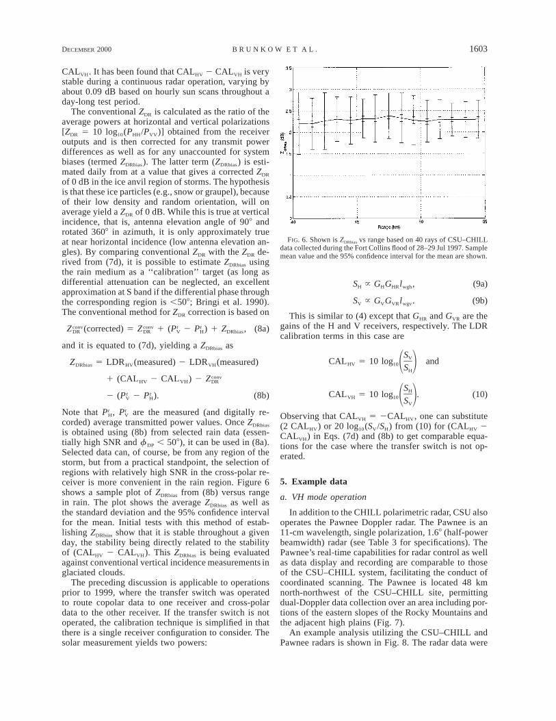
FIG. 6. Shown is ZDRbias vs range based on 40 rays of CSU–CHILLdata collected during the Fort Collins flood of 28–29 Jul 1997. Samplemean value and the 95% confidence interval for the mean are shown.

CALVH. It has been found that CALHV 2 CALVH is verystable during a continuous radar operation, varying byabout 0.09 dB based on hourly sun scans throughout aday-long test period.

The conventional ZDR is calculated as the ratio of theaverage powers at horizontal and vertical polarizations[ZDR 5 10 log10(PHH/PVV)] obtained from the receiveroutputs and is then corrected for any transmit powerdifferences as well as for any unaccounted for systembiases (termed ZDRbias). The latter term (ZDRbias) is esti-mated daily from at a value that gives a corrected ZDR

of 0 dB in the ice anvil region of storms. The hypothesisis that these ice particles (e.g., snow or graupel), becauseof their low density and random orientation, will onaverage yield a ZDR of 0 dB. While this is true at verticalincidence, that is, antenna elevation angle of 908 androtated 3608 in azimuth, it is only approximately trueat near horizontal incidence (low antenna elevation an-gles). By comparing conventional ZDR with the ZDR de-rived from (7d), it is possible to estimate ZDRbias usingthe rain medium as a ‘‘calibration’’ target (as long asdifferential attenuation can be neglected, an excellentapproximation at S band if the differential phase throughthe corresponding region is ,508; Bringi et al. 1990).The conventional method for ZDR correction is based on

5 1 ( 2 ) 1 ZDRbias,conv conv t tZ (corrected) Z P PDR DR V H (8a)

and it is equated to (7d), yielding a ZDRbias as

ZDRbias 5 LDRHV(measured) 2 LDRVH(measured)

1 (CALHV 2 CALVH) 2 convZDR

2 ( 2 ).t tP PV H (8b)

Note that , are the measured (and digitally re-t tP PH V

corded) average transmitted power values. Once ZDRbias

is obtained using (8b) from selected rain data (essen-tially high SNR and f DP , 508), it can be used in (8a).Selected data can, of course, be from any region of thestorm, but from a practical standpoint, the selection ofregions with relatively high SNR in the cross-polar re-ceiver is more convenient in the rain region. Figure 6shows a sample plot of ZDRbias from (8b) versus rangein rain. The plot shows the average ZDRbias as well asthe standard deviation and the 95% confidence intervalfor the mean. Initial tests with this method of estab-lishing ZDRbias show that it is stable throughout a givenday, the stability being directly related to the stabilityof (CALHV 2 CALVH). This ZDRbias is being evaluatedagainst conventional vertical incidence measurements inglaciated clouds.

The preceding discussion is applicable to operationsprior to 1999, where the transfer switch was operatedto route copolar data to one receiver and cross-polardata to the other receiver. If the transfer switch is notoperated, the calibration technique is simplified in thatthere is a single receiver configuration to consider. Thesolar measurement yields two powers:

S } G G l , (9a)H H HR wgh

S } G G l . (9b)V V VR wgv

This is similar to (4) except that GHR and GVR are thegains of the H and V receivers, respectively. The LDRcalibration terms in this case are

SVCAL 5 10 log andHV 101 2SH

SHCAL 5 10 log . (10)VH 101 2SV

Observing that CALVH 5 2CALHV, one can substitute(2 CALHV) or 20 log10(SV/SH) from (10) for (CALHV 2CALVH) in Eqs. (7d) and (8b) to get comparable equa-tions for the case where the transfer switch is not op-erated.

5. Example data

a. VH mode operation

In addition to the CHILL polarimetric radar, CSU alsooperates the Pawnee Doppler radar. The Pawnee is an11-cm wavelength, single polarization, 1.68 (half-powerbeamwidth) radar (see Table 3 for specifications). ThePawnee’s real-time capabilities for radar control as wellas data display and recording are comparable to thoseof the CSU–CHILL system, facilitating the conduct ofcoordinated scanning. The Pawnee is located 48 kmnorth-northwest of the CSU–CHILL site, permittingdual-Doppler data collection over an area including por-tions of the eastern slopes of the Rocky Mountains andthe adjacent high plains (Fig. 7).

An example analysis utilizing the CSU–CHILL andPawnee radars is shown in Fig. 8. The radar data were


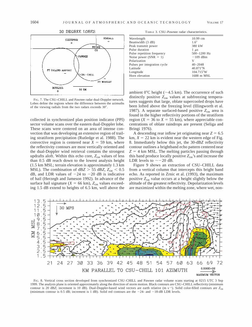
FIG. 7. The CSU–CHILL and Pawnee radar dual-Doppler network.Lobes define the regions where the difference between the azimuthsof the viewing radials from the two radars exceeds 308.

TABLE 3. CSU–Pawnee radar characteristics.

WavelengthBeamwidth (3 dB)Peak transmit powerPulse durationPulse repetition frequency

10.99 cm1.68380 kW1 ms500–1200 Hz

Noise power (SNR 5 1)PolarizationPulses per integration cycleLatitudeLongitudeHorn elevation

2109 dBmV40–204840.8718N104.7158W1688 m MSL

FIG. 8. Vertical cross section developed from synchronized CSU–CHILL and Pawnee radar volume scans starting at 0215 UTC 3 Sep1999. The analysis plane is oriented approximately along the direction of storm motion. Black contours are CSU–CHILL reflectivity (minimumcontour is 20 dBZ; increment is 10 dB). Dual-Doppler-based wind vectors are earth relative (m s21). Solid color-filled contours are ZDR

(minimum contour is 0.5 dB; increment is 1 dB). Solid red contours are the 224- and 218-dB LDR levels.

collected in synchronized plan position indicator (PPI)sector volume scans over the eastern dual-Doppler lobe.These scans were centered on an area of intense con-vection that was developing an extensive region of trail-ing stratiform precipitation (Rutledge et al. 1988). Theconvective region is centered near X 5 59 km, wherethe reflectivity contours are most vertically oriented andthe dual-Doppler wind retrieval contains the strongestupdrafts aloft. Within this echo core, ZDR values of lessthan 0.5 dB reach down to the lowest analysis height(1.5 km MSL; terrain elevation is approximately 1.3 kmMSL). The combination of dBZ . 55 dBZ, ZDR , 0.5dB, and LDR values of 224 to 220 dB is indicativeof hail (Herzegh and Jameson 1992). In advance of thesurface hail signature (X 5 66 km), ZDR values exceed-ing 1.5 dB extend to heights of 6.5 km, well above the

ambient 08C height (;4.5 km). The occurrence of suchdistinctly positive ZDR values at subfreezing tempera-tures suggests that large, oblate supercooled drops havebeen lofted above the freezing level (Illingworth et al.1987). A separate surfaced-based positive ZDR area isfound in the higher reflectivity portions of the stratiformregion (X 5 36 to X 5 55 km), where appreciable con-centrations of oblate raindrops are present (Seliga andBringi 1976).

A descending rear inflow jet originating near Z 5 6.5km, X 5 22 km is evident near the western edge of Fig.8. Immediately below this jet, the 30-dBZ reflectivitycontour outlines a brightband echo pattern centered nearZ 5 4 km MSL. The melting particles passing throughthis band produce locally positive ZDR’s and increase theLDR levels to ;220 dB.

Figure 9 shows an extraction of CSU–CHILL datafrom a vertical column that intercepts this bright bandecho. As reported in Zrnic et al. (1993), the maximumpositive ZDR value occurs at a height slightly below thealtitude of the greatest reflectivity. Depolarization levelsare maximized within the melting zone, where wet, non-


FIG. 9. CSU–CHILL data vertical profiles through a bright bandas extracted from the volume scan starting at 0215 UTC 3 Sep 1999.The plotted data are range averages over the three consecutive gatesin each PPI sweep that are centered nearest to an azimuth of 1018and a range of 20 km. The profiles are annotated with selected datavalues. Reference values are shown with dashed vertical lines: 0 dBin the ZDR panel; 0.99 and 1.00 correlations in the rHV panel.

spherical ice particles with fluctuating orientations aremost likely to be present (Illingworth and Caylor 1989).LDR levels are distinctly low (often less than ;230dB) at heights outside of the melting zone. Similarly,rHV values are quite high (0.99 to 1.0), except withinthe melting zone, where both irregularly shaped ice par-ticles and melted drops coexist (Balakrishnan and Zrnic1990; Zrnic et al. 1993).

b. Hybrid basis mode

We mentioned in section 2a that the transmitters maybe triggered either alternately or simultaneously. Withthe alternate VH mode, the conventional estimates ofZDR, f DP, and rHV are formed from the copolar HH andVV signals available at the input to the digital receiverson the even and odd pulse intervals, respectively. Atthe same time, the cross-polar VH and VH signals areavailable at the input to the opposite receiver. Thisscheme is based on the classical orthogonal basis.

When the transmitters are triggered simultaneouslywith matched power outputs, the radiated polarizationstate can be described by the unit vector

juh 1 e ve 5 , (11)

Ï2

where u is the phase difference between the two transmitchannels. While u can be controlled via an I/Q vectormodulator, for the purposes of this discussion, u will betreated as an unknown but fixed system constant. Thetwo receivers are used to measure the elements of thecoherency matrix, defined as

r r r rÊ E *& Ê E *&H H H VJ 5 , (12)r r r r[ ]Ê E *& Ê E *&V H V V

where and are the horizontal and vertical polar-r rE EH V

ized components of the backscattered ellipse, a doublebar indicating a matrix. Since the solid state transferswitch is not activated in this mode, the horizontallypolarized component is received by the first receiverand the vertically polarized component is received bythe second receiver. The ZDR, cDP, and rHV in this hybridmode are obtained as

r 2^|E | &HhyZ 5 10 log , (13a)DR 10 r 2[ ]^|E | &V

hy r rC 5 arg(Ê * E &), (13b)DP H V

r r|Ê * E &|H Vhyr 5 . (13c)HVr 2 r 2Ï^|E | &^|E | &H V

Angle brackets denote time averages. This measurementscheme is termed the hybrid basis as opposed to theclassical orthogonal basis described in the beginning ofthis section. It is interesting to note that both schemeswere suggested by Seliga and Bringi (1976) as possiblefor ZDR measurements.

Measurements in the hybrid basis will, in principle,lead to no error if the propagation and scattering ma-trices are diagonal, since the received electric field com-ponents can be expressed as

r l r l r1 1E Z GP 1 e 0 S 0 e 0H 0 t HH5r 2 l r l r2 2[ ] [ ][ ][ ]!E 2p r 0 e 0 S 0 eV VV

1

Ï23 , (14)

1jue Ï2

where l1 and l2 are the eigenvalues of the propagationmedium (Oguchi 1983); SHH and SVV are elements of thescattering matrix of the resolution volume centered atrange r; and Z0, G, and Pt are the intrinsic impedanceof vacuum, antenna gain, and peak transmitted power,respectively. If the propagation medium is nonatten-uating and imposes a pure differential phase (a goodapproximation for propagation in rain at S band), thenit is easily verified that (e.g., Sachidananda and Zrnic1985)

2^|S | &HHhyZ 5 10 log , (15a)DR 10 2[ ]^|S | &VV

hyC 5 arg(^S* S &) 1 F 1 u 5 F 1 u, (15b)DP HH VV DP DP

|^S* S &|HH VVhyr 5 , (15c)co2 2Ï^|S | &^|S | &HH VV


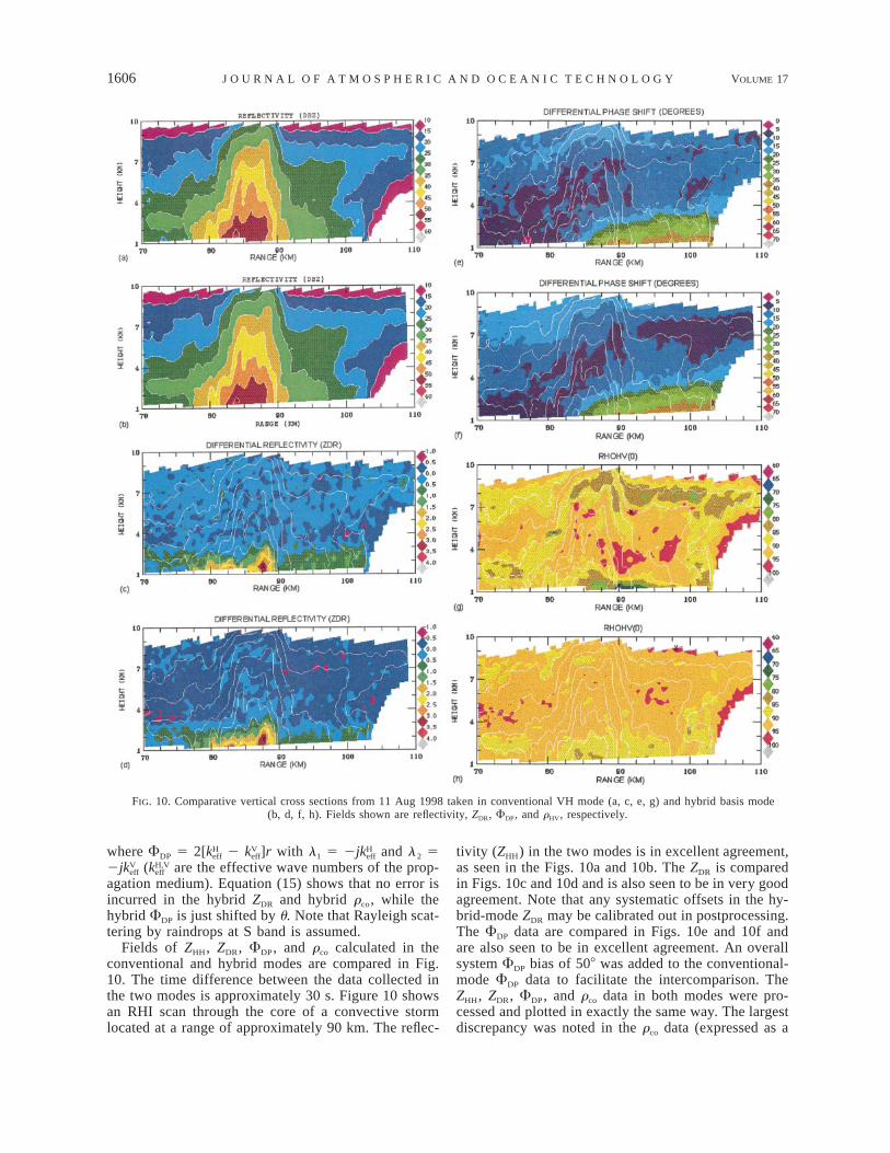
FIG. 10. Comparative vertical cross sections from 11 Aug 1998 taken in conventional VH mode (a, c, e, g) and hybrid basis mode(b, d, f, h). Fields shown are reflectivity, ZDR, FDP, and rHV, respectively.

where FDP 5 2[ 2 ]r with l1 5 2 and l2 5H V Hk k jkeff eff eff

2 ( are the effective wave numbers of the prop-V H,Vjk keff eff

agation medium). Equation (15) shows that no error isincurred in the hybrid ZDR and hybrid rco, while thehybrid FDP is just shifted by u. Note that Rayleigh scat-tering by raindrops at S band is assumed.

Fields of ZHH, ZDR, FDP, and rco calculated in theconventional and hybrid modes are compared in Fig.10. The time difference between the data collected inthe two modes is approximately 30 s. Figure 10 showsan RHI scan through the core of a convective stormlocated at a range of approximately 90 km. The reflec-

tivity (ZHH) in the two modes is in excellent agreement,as seen in the Figs. 10a and 10b. The ZDR is comparedin Figs. 10c and 10d and is also seen to be in very goodagreement. Note that any systematic offsets in the hy-brid-mode ZDR may be calibrated out in postprocessing.The FDP data are compared in Figs. 10e and 10f andare also seen to be in excellent agreement. An overallsystem FDP bias of 508 was added to the conventional-mode FDP data to facilitate the intercomparison. TheZHH, ZDR, FDP, and rco data in both modes were pro-cessed and plotted in exactly the same way. The largestdiscrepancy was noted in the rco data (expressed as a


percentage) from the two modes, as shown in Figs.10g–h. The conventional mode rco is seen to be lower,particularly within the highest reflectivity region near1-km height and also near the storm top. It is knownfrom simulations that the conventional-mode rco will bebiased low (by 5%–15%) when the Doppler spectralshape is not Gaussian (either very broad shape or spectrawith multiple peaks; Liu et al. 1994), which can likelyoccur in severe storms. On the other hand, the hybrid-mode rco can be biased low due to the so-called back-scatter depolarization effect modeled by Doviak et al.(2000). This tendency does not stand out when com-paring Figs. 10g and 10h, though it may be noted neara range of 90 km and a height of 3 km, where conven-tional rco is around 95%–100% whereas the hybrid-mode rco is 85%–95%. These initial data comparisonssuggest that the hybrid scheme should be further ex-plored for application to operational radar systems(Doviak et al. 2000).

6. Overview of the CSU–CHILL facility

a. Radar packaging and transportability

The CSU–CHILL system is designed to be moved tosupport data collection at locations other than the homebase near Greeley, Colorado. The entire radar system istransportable on five 14.6-m-long (48 ft) semitrailers.Only three of these trailers (the transmitter, user, andequipment storage vans) need to be at the radar siteduring operations. The forward portion of the user vanprovides an 8.5 m by 2.1 m (28 ft by 7 ft) controlledenvironment space from which real-time radar opera-tions are directed (Mueller et al. 1995). This user areaalso has ample space to accommodate special project-related equipment (radios, additional workstations, etc.).

The CSU–CHILL antenna is protected by an air-in-flated radome constructed of reinforced nylon material.This radome has an equatorial diameter of 22.3 m anda maximum height of 16.2 m. Support for the combinedantenna pedestal and radome system is provided by a19.8-m-diameter reinforced concrete foundation. Thisfoundation was recently redesigned to decrease theamount of concrete needed, thereby significantly re-ducing the cost of the pad installation. Additional detailsconcerning the remote deployment of the system maybe obtained at the facility Web site.

b. Real-time radar operation and data dissemination

Real-time operation of the CSU–CHILL system isdone via fully interactive control software. The specificdata collection parameters (antenna scan angular limits,transmitter pulse repetition frequency, etc.) are collectedinto an arbitrary number of predefined scan segments,which are loaded from computer files as needed. Thesegment parameters may also be easily modified duringoperations. PPI scan optimization is optionally per-

formed while the scan is in progress. If enabled, thescan optimizer chooses each elevation scan angle basedon minimum spatial resolution requirements establishedby the operator. Each scan segment describes the signalprocessor and radar operating parameters as well as thebasic antenna motion (i.e., which axis is scanning, scanrate, scan limits, etc.). These scan segments may beactivated in an arbitrary order by the operator or linkedtogether to define a repeating sequence of scans. Timerscan be established to start specific scan segments atspecific times and/or recurrence intervals. This radarcontrol arrangement readily permits the data acquisitionscheme to be synchronized with other radars and to beadapted as the echoes of interest evolve and move.

Color displays of the radar data fields are availablein real time on a ray-by-ray basis in the user van. Se-lected color display images (typically four data fieldsfrom one sweep in a particular scan segment) can betransferred onto the CSU–CHILL Web site. These savedimages are available for viewing within seconds of thecompletion of the sweep to be saved. Also, Internetcommunication techniques are under development thatwill permit investigators who are not physically at theuser van to access the radar’s real-time data acquisitionparameters and to input scan modifications. Thus, it isanticipated that in the near future, researchers will beable to remotely direct real-time CSU–CHILL opera-tions.

All CSU–CHILL data are routinely recorded on 8-mmmagnetic tape cartridges. These field tapes may easilybe replayed through the radar’s color display system.Copies of the archived data may also be rapidly con-verted to various ‘‘standard’’ formats, including Uni-versal Doppler Exchange Format (Barnes 1980).

7. Summary

As presently configured, the CSU–CHILL is a trans-portable S-band radar system providing an instrumentfor the collection of research-quality multiparameter ra-dar data. With the dual-transmitter and dual-receiverconfiguration, maximum polarimetric performance isobtained from a prime-focus reflector antenna. The re-cent upgrade of the radar’s data processing system willpermit the antenna scan rate to be nearly doubled whilemultiparameter data are being collected.

An immediate application of this performance im-provement will be the collection of higher time reso-lution dual-Doppler and polarimetric datasets using theCSU–CHILL and Pawnee radar network. It is expectedthat the resultant high time resolution, combined dual-Doppler, and multiparameter radar datasets will providenew insights into storm dynamics, precipitation pro-cesses, and cloud electrification mechanisms.

Prospective radar users should consult the facility’sWeb site (http://chill.colostate.edu) for access to ar-chived data as well as current facility information.


Acknowledgments. Mr. Gwo-Jong Huang performedthe antenna pattern convolution modeling runs. TheCSU–CHILL National Radar Facility is sponsored bythe National Science Foundation under Grant ATM-9500108 and by Colorado State University. SAR, VNB,and VC also acknowledge support from the U.S. Weath-er Research Program via the NSF under Grant ATM-9612519. Expert technical support of the facility wasalso provided by Kenneth Pattison.

REFERENCES

Aydin, K., T. A. Seliga, and B. Balaji, 1986: Remote sensing of hailwith a dual linear polarization radar. J. Climate Appl. Meteor.,25, 1475–1481.

Balakrishnan, N., and D. S. Zrnic, 1990: Use of polarization to char-acterize precipitation and discriminate large hail. J. Atmos. Sci.,47, 1525–1540

Barnes, S. L., 1980: Report on a meeting to establish a commonDoppler radar data exchange format. Bull. Amer. Meteor. Soc.,61, 1401–1404.

Blanchard, J., and R. W. Newton, 1985: Demands on polarizationpurity in the measurement and imaging of distributed clutter.Mathematical and Physical Sciences, W. Boerner, Ed., NATOASI Series C, Vol. 153, D. Reidel, 721–738.

Bringi, V. N., and A. Hendry, 1990: Technology of polarization di-versity radars for meteorology. Radar in Meteorology, D. Atlas,Ed., Amer. Meteor. Soc., 153–190., V. Chandrasekar, N. Balakrishnan, and D. S. Zrnic, 1990: Anexamination of propogation effects in rainfall on radar mea-surements at microwave frequencies. J. Atmos. Oceanic Tech-nol., 7, 829–840

Carter, J. K., D. Sirmans, and J. Schmidt, 1986: Engineering descrip-tion of the NSSL dual linear polarization Doppler weather radar.Preprints, 23d Radar Meteorology Conf., Snowmass, CO, Amer.Meteor. Soc., 381–384.

Doviak, R. I., and D. S. Zrnic, 1993: Doppler Radar and WeatherObservations. Academic Press, 562 pp., V. Bringi, A. Ryzhkov, A. Zahari, and D. S. Zrnic, 2000: Con-siderations for polarimetric upgrades to operational WSR-88Dradars. J. Atmos. Oceanic Technol., 17, 257–278.

Herzegh, P. H., and R. E. Carbone, 1984: The influence of antennaillumination function characteristics on differential reflectivitymeasurements. Preprints, 22d Radar Meteorology Conf., Zurich,Switzerland, Amer. Meteor. Soc., 281–286., and A. R. Jameson, 1992: Observing precipitation formationthrough dual-polarization radar measurements. Bull. Amer. Me-teor. Soc., 73, 1365–1374.

Hubbert, J., V. N. Bringi, L. D. Carey, and S. Bolen, 1998: CSU–CHILL polarimetric radar measurements from a severe hailstormin eastern Colorado. J. Appl. Meteor., 37, 749–775.

Illingworth, A. J., and I. J. Caylor, 1989: Cross polar observationsof the bright band. Preprints, 24th Conf. on Radar Meteorology,Tallahassee, FL, Amer. Meteor. Soc., 323–327., J. W. F. Goddard, and S. M. Cherry, 1987: Polarization radarstudies of precipitation development in convective storms.Quart. J. Roy. Meteor. Soc., 113, 469–489.

Jameson, A. R., 1985: On deducing the microphysical character ofprecipitation from multiple-parameter radar polarization mea-surements. J. Climate Appl. Meteor., 24, 1037–1047.

, and D. B. Johnson, 1990: Cloud microphysics and radar.Radar in Meteorology, D. Atlas, Ed., Amer. Meteor. Soc., 323–347.

Liu, L., V. N. Bringi, V. Chandrasekar, E. A. Mueller, and A. Mu-dukutore, 1994: Analysis of the co-polar correlation coefficientbetween horizontal and vertical polarizations. J. Atmos. OceanicTechnol., 11, 950–963.

McCormick, G. C., 1981: Polarization errors in a two channel system.Radio Sci., 16, 67–75., and A. Hendry, 1975: Principles for the radar determination ofthe polarization properties of precipitation. Radio Sci., 10, 421–434., and , 1979: Techniques for the determination of the po-larization properties of precipitation. Radio Sci., 14, 1027–1040.

Mueller, E. A., 1981: Implementation of differential reflectivity onthe CHILL radar. Preprints, 20th Radar Meteorology Conf., Bos-ton, MA, Amer. Meteor. Soc., 666–667., and E. J. Silha, 1978: Unique features of the CHILL radarsystem. Preprints, 18th Radar Meteorology Conf., Atlanta, GA,Amer. Meteor. Soc., 381–382., S. A. Rutledge, V. N. Bringi, D. Brunkow, P. C. Kennedy, K.Pattison, R. Bowie, and V. Chandrasekar, 1995: CSU–CHILLradar upgrades. Preprints, 27th Radar Meteorology Conf., Vail,CO, Amer. Meteor. Soc., 703–706.

Oguchi, T., 1983: Electromagnetic wave propagation and scatteringin rain and other hydrometeors. Proc. IEEE, 71, 1029–1078.

Petersen, W. A., and Coauthors, 1999: Mesoscale and radar obser-vations of the Fort Collins flash flood of 28 July 1997. Bull.Amer. Meteor. Soc., 80, 191–216.

Pointin, Y., D. Ramond, and J. Fournet-Fayard, 1988: Radar differ-ential reflectivity ZDR: A real-case evaluation of errors inducedby antenna characteristics. J. Atmos. Oceanic Technol., 5, 416–423.

Rutledge, S. A., R. A. Houze Jr., M. I. Biggerstaff, and T. Matejka,1988: The Oklahoma–Kansas mesoscale convective system of10–11 June 1985: Precipitation structure and single-Doppler ra-dar analysis. Mon. Wea. Rev., 116, 1409–1430.

Sachidananda, M., and D. S. Zrnic 1985: ZDR measurement consid-eration for a fast scan capability radar. Radio Sci., 20, 907–922.

Seliga, T. A., and V. N. Bringi, 1976: Potential use of radar differentialreflectivity measurements at orthogonal polarizations for mea-suring precipitation. J. Appl. Meteor., 15, 69–76.

Tragl, K., 1990: Polarimetric radar backscattering from reciprocalrandom targets. IEEE Trans. Geosci. Remote Sens., 8, 856–864.

Ussailis, J. S., and J. I. Metcalf, 1983: Analysis of a polarizationdiversity meteorological radar design. Preprints, 21st Radar Me-teorology Conf., Edmonton, AB, Canada, Amer. Meteor. Soc.,331–338.

Wood, P. J., 1980: Reflector Antenna Analysis and Design. Peregrinus,226 pp.

Wu, Y., 1998: Design of digital radar receivers. IEEE Aerospace andElectronic Systems Magazine Vol. 8, No. 1, 35–41.

Zrnic, D. S., N. Balakrishnan, C. L. Ziegler, V. N. Bringi, K. Aydin,and T. Matejka, 1993: Polarimeteric signatures in the stratiformregion of a mesoscale convective system. J. Appl. Meteor., 32,678–693.

Documents

1596 JOURNAL OF ATMOSPHERIC AND …radarmet.atmos.colostate.edu/pdf/CHILLDescip.pdf1596 JOURNAL OF ATMOSPHERIC AND OCEANIC TECHNOLOGY VOLUME 17 q 2000 American Meteorological Society