Embed Size (px)
Citation preview

12
Robust Control of a Rocket
In this chapter we consider the design of a robust system for attitude sta-bilisation of a winged supersonic rocket flying at altitudes between 1000 mand 10000 m. The plant to be controlled is timevariant, which makes thecontroller design difficult. To simplify the design, we first derive linearisedequations of the longitudinal motion of the rocket. Variations of the aerody-namic coefficients of this motion are considered as parametric uncertainties inthe design. In this study, both continuous-time and discrete-time μ-controllersare designed that are implemented for pitch and yaw control and ensure thedesired closed-loop dynamics in the presence of uncertainty, disturbances andnoises. Robust stability and robust performance of the closed-loop systemswith the implementation of each controller are investigated, respectively, andthe nonlinear closed-loop, sampled-data system simulation results are given.
12.1 Rocket Dynamics
We consider a winged rocket that has a canard aerodynamic configurationand is equipped with a solid propellant engine. The actuators of the attitude-stabilization system in the longitudinal and lateral motions are four controlsurfaces (fins) that may rotate in pairs about their axes. The roll angle stabil-isation is realised by auxiliary surfaces (ailerons). The control aim is to ensureaccurate tracking of required acceleration maneuvers in the presence of un-certainties in the aerodynamic characteristics, disturbances (wind gusts) andsensor noises. The controller produces the inputs to two servo-actuators thatrotate the fins. The normal acceleration in each plane and the pitch (yaw)rate are measured, respectively, by an accelerometer and a rate gyro, and arefeedback signals to the controller.
To describe the rocket motion in space we shall need three orthogonalreference frames: the vehicle-carried vertical reference frame, the body-fixedreference frame and the flight-path reference frame. These three referenceframes all have their origin in the rocket’s mass centre.

290 12 Robust Control of a Rocket
Fig. 12.1. Relationship between the vehicle-carried vertical reference frame and thebody-fixed reference frame
The x∗-axis of the vehicle-carried vertical reference frame is directed to theNorth, the y∗-axis to the East, and the z∗-axis points downwards along thelocal direction of the gravity. The x1-axis of the body-fixed reference frameis directed towards to the nose of the rocket, the y1-axis points to the topwing, and the z1-axis points to the right wing. In Figure 12.1 we show therelationship between the vehicle-carried vertical reference frame O∗x∗y∗z∗ andthe body-fixed reference frame Ox1y1z1. The rocket attitude (i.e. the positionof the frame Ox1y1z1 with respect to O∗x∗y∗z∗) is characterised by the anglesϑ, ψ, γ that are called pitch angle, yaw angle, and roll angle, respectively.The value of the roll angle in the nominal motion is usually very small.
The x-axis of the flight-path reference frame is aligned with the velocityvector V of the rocket and the y-axis lies in the plane Ox1y1. The relationshipbetween the body-fixed reference frame and the flight-path reference frame isshown in Figure 12.2. The orientation of the body-fixed reference frame withrespect to the flight-path reference frame is determined by the angle of attackα and the sideslip angle β.
Finally, the relationship between the vehicle-carried vertical referenceframe O∗x∗y∗z∗ and the flight-path reference frame Oxyz is shown in Figure12.3. The position of the frame Oxyz with respect to O∗x∗y∗z∗ is determined

12.1 Rocket Dynamics 291
Fig. 12.2. Relationship between the body-fixed reference frame and the flight-pathreference frame
by the flight-path angle Θ, the bank angle Ψ and the aerodynamic angle ofroll γc.
The characteristic points along the longitudinal body axis of the rocketare shown in Figure 12.4, where
xG is the coordinate of the mass centre of the rocket;xC is the coordinate of the aerodynamic centre of pressure (the point where
the aerodynamic forces are applied upon);xR is the coordinate of the fins rotation axis.The rocket will be statically stable or unstable depending on the location
of the centre of pressure relative to the centre of mass. If xG < xC then therocket is statically stable.
The control of the lateral acceleration of the rocket is carried out in thefollowing way. The moments about the mass centre, due to the fins deflections,create the corresponding angle of attack and sideslip angle. These angles, inturn, lead to the lifting forces and accelerations in the corresponding planes.The control problem consists of generation of the fins deflections by the au-topilot that produce angle of attack and sideslip angle, corresponding to amaneuver called for by the guidance law, while stabilising the rocket rota-tional motion.
The nonlinear differential and algebraic equations describing the six degree-of-freedom motion of the rocket are as follows.

292 12 Robust Control of a Rocket
Fig. 12.3. Relationship between the vehicle-carried vertical reference frame and theflight-path reference frame
Fig. 12.4. Coordinates of the characteristic points of the body
1. Equations describing the motion of the mass centre
mV = P cos α cos β − Q − G sinΘ + Fx(t)mV Θ = P (sinα cos γc + cos α sin β sin γc)
+Y cos γc − Z sin γc − G cos Θ + Fy(t) (12.1)
−mV cos ΘΨ = P (sinα sin γc − cos α sinβ cos γc)

12.1 Rocket Dynamics 293
+Y sin γc + Z cos γc + Fz(t)
In these equations, P is the engine thrust, Q is the drag force, Y andZ are the lift forces in directions y and z, respectively, G = mg is therocket weight (g = 9.80665 m/s2 is the acceleration of gravity at sealevel), Fx(t), Fy(t), Fz(t) are generalised disturbance forces in directionsx, y, z, respectively. Also, m is the mass of the rocket in the currentmoment of the time.The engine thrust is given by P = P0 +(p0 −p)Sa, where P0 is the enginethrust at the sea level, p0 = 101325 N/m2 is the atmospheric pressure atthe sea level, p is the pressure at the flight altitude, and Sa is the area ofthe engine nozzle output section. It is assumed that the mass consumptionrate μ of the propellant remains constant, i.e. P0 = const.Further, let S and L be the reference area and the length of the rocketbody, respectively and let q = ρV 2
2 be the dynamic pressure, where ρ isthe air density at the corresponding altitude. Then,Q = Qa + Qc, where Qa = cxqS is the drag force of the body and wings,Qc = (cδy
x |δy| + cδzx |δz|)qS is the drag force due to the fins deflections,
δy, δz are the angles of the fins deflection in the longitudinal and lateralmotion, respectively, and cx, c
δyx , cδz
x are dimensionless coefficients;Y = Ya + Yc, where Ya = cyqS is the lift force of the body and wings,Yc = cδz
y δzqS is the lift force due to the deflection of the horizontal fins,cy = cα
y α and cαy is a dimensionless coefficient. Similar expressions hold for
the lift force Z: Z = Za + Zc, Za = czqS, Zc = cδyz δyqS, where cz = cβ
z β.Due to the rocket symmetry cβ
z = −cαy , c
δyz = −cδz
y .The aerodynamic coefficients cx, c
δyx , cδz
x , cαy , cβ
z depend on the rocketgeometry as well as on the Mach number M = V
a , where a is the soundspeed at the corresponding altitude. These coefficients are determined byapproximate formulae and are defined more precisely using experimentaldata.
2. Equations, describing the rotational motion about the mass centre
Ixωx + (Iz − Iy)ωyωz = Mfx + Md
x + M cx + Mx(t)
Iyωy + (Ix − Iz)ωzωx = Mfy + Md
y + M cy + My(t) (12.2)
Izωz + (Iy − Ix)ωxωy = Mfz + Md
z + M cz + Mz(t)
ψ = (ωy cos γ − ωz sin γ)/ cos θ
θ = ωy sin γ + ωz cos γ (12.3)γ = ωx − tan θ(ωy cos γ − ωz sin γ)
In these equations, Ix, Iy, Iz are the rocket moments of inertia; Mfx , Mf
y ,Mf
z are aerodynamic moments due to the angle of attack α and the sideslip

294 12 Robust Control of a Rocket
angle β; Mdx , Md
y , Mdz are aerodynamic damping moments due to the roll,
pitch and yaw rates ωx, ωz, ωy, respectively; M cx, M c
y , M cz are control
moments due to the fins deflections δx, δy, δz, respectively, and Mx(t),My(t), Mz(t) are generalised disturbance moments about correspondingaxes. We have that• Mf
x = (mαxα + mβ
xβ)qSL; Mfy = mβ
yβqSL; Mfz = mα
z αqSL, wheremα
x , mβx , mβ
y , mαz are dimensionless coefficients;
• Mdx = mωx
x ωxqSL2/V, Mdy = m
ωyy ωyqSL2/V, Md
z = mωzz ωzqSL2/V ,
where mωxx , m
ωyy , mωz
z are dimensionless coefficients;• M c
x = mδxx δxqSL, M c
y = mδyy δyqSL, M c
z = mδzz δzqSL, where mδx
x ,m
δyy , mδz
z are dimensionless coefficients. For the given rocket configura-tion it is fulfilled that M c
y = Zc(xG−xR) cos β, M cz = Yc(xG−xR) cos α
so that mδyy = −c
δyz (xG − xR)/L cos β, mδz
z = cδzy (xG − xR)/L cos α.
3. Equations providing the relationships between the angles ψ, θ, γ, α, β,Ψ, Θ, γc
sin β = (sin θ sin γ cos(Ψ − ψ) − cos γ sin(Ψ − ψ)) cos Θ
− cos θ sin γ sin Θ
sin α = ((sin θ cos γ cos(Ψ − ψ) + sin γ sin(Ψ − ψ)) cos Θ (12.4)− cos θ cos γ sinΘ)/ cos β
sin γc = (cos α sin β sin θ − (sin α sinβ cos γ − cos β sin γ) cos θ)/ cos Θ
4. Equations providing the accelerations nx1, ny1, nz1 in the body-fixed ref-erence frame
nx1 = nx cos α cos β + ny sin α − nz cos α sin β
ny1 = −nx sin α cos β + ny cos α + nz sinα sin β (12.5)nz1 = nx sinβ + nz cos β
where the accelerations nx, ny, nz in the flight-path reference frame aregiven by
nx = (P cos α cos β − Q)/G
ny = (P sin α + Y )/G
nz = (−P cos α sin β + Z)/G
Note that the accelerations ny1, nz1 are measured by accelerometers fixedwith the axes y1, z1, respectively. For brevity, later instead of ny1, nz1
we shall write ny, nz.Equations (12.1) – (12.5) are used later in the simulation of the nonlinearrocket stabilization system.
For small deviations from the nominal(unperturbed) motion, the three-dimensional motion of the rocket can be decomposed with sufficient accuracy

12.1 Rocket Dynamics 295
in three independent motions – pitch, yaw and roll. In the controller design, weconsider only the pitch perturbation motion. In this case the rocket attitudeis characterised by the angles Θ and θ (or, equivalently, α and θ). Due tothe rocket symmetry the yaw stabilisation system is analogous to the pitchstabilisation system.
Fig. 12.5. Force diagram in the vertical plane
The equations describing the rocket’s longitudinal motion have the form(Figure 12.5).
1. Equations describing the motion of the mass centreThese equations are obtained from (12.1) by substituting β = 0, γc = 0.
mV = P cos α − Q − G sin Θ + Fx(t) (12.6)
mV Θ = P sinα + Y − G cos Θ + Fy(t) (12.7)
2. Equations, describing the rotational motion about the mass centreThese equations are obtained from (12.2) and (12.3) by substituting ωx =0, ωy = 0, γ = 0.
Izωz = Mfz + Md
z + M cz + Mz(t) (12.8)
θ = ωz

296 12 Robust Control of a Rocket
3. Equation giving the relationships between the angles α, θ, ΘThis equation is obtained from (12.4) for Ψ = 0, ψ = 0.
α = θ − Θ (12.9)
4. Equation giving the normal acceleration ny
This equation is obtained from (12.5) for β = 0.
ny = −P cos α − Q
Gsin α +
P sin α + Y
Gcos α (12.10)
Later, it is assumed that the rocket velocity V (or Mach number) isconstant and the nonlinear differential equation (12.6) associated with V isdropped from the design model. This assumption is justified by the resultsfrom the nonlinear system simulation presented later. Also, as is often cus-tomary, we shall neglect the effect of the gravitational force in (12.7).
In order to obtain a linear controller (12.7) – (12.10) are linearised abouttrim operating points (Θ = Θo, θ = θo, α = αo, ωz = ωo
z , δz = δoz) under
the assumptions that the variations ΔΘ = Θ − Θo, Δθ = θ − θo, Δα =α − αo, Δωz = ωz − ωo
z , Δδz = δz − δoz are sufficiently small. In such a case
it is fulfilled that sinΔα ≈ Δα, cos α ≈ 1.As a result, the linearised equations of the perturbed motion of the rocket
take the form (for convenience the symbol Δ is omitted)
Θ =P + Y α
mVα +
Y δz
mVδz +
Fy(t)mV
ωz =Mα
z
Jzα +
Mωzz
Jzωz +
M δzz
Jzδz +
Mz(t)Jz
θ = ωz (12.11)α = θ − Θ
ny =Q + Y α
Gα +
Y δz
Gδz
where Y α = cαy qS, Y δz = cδz
y qS, Mαz = mα
z qSL, Mωzz = mωz
z qSL2/V, M δzz =
mδzz δzqSL.Equations (12.11) are represented as
Θ = aΘΘα + aΘδz+ F y(t)
θ = aθθ θ + aθθα + aθδzδz + Mz(t) (12.12)
α = θ − Θ
ny = anyαα + anyδzδz
whereaΘΘ = P+Y α
mV , aΘδz = Y δz
mV
aθθ = Mωzz
Jz, aθθ = Mα
z
Jz
aθδz = Mδzz
Jz, anyα = Q+Y α
G
anyδz = Y δz
G

12.1 Rocket Dynamics 297
In (12.12) we used the notation
Fy(t) =Fy(t)mV
and
Mz(t) =Mz(t)
J
Equations (12.12) are extended by the equation describing the rotation ofthe fins
δz + 2ξδzωδz
δz + ω2δz
δz = ω2δz
δoz (12.13)
where δoz is the desired angle of fin’s deflection (the servo-actuator reference),
ωδzis the natural frequency and ξδz
the damping coefficient of the servo-actuator.
The set of equations (12.12) and (12.13) describes the perturbed rocketlongitudinal motion.
The block diagram of the stabilisation system, based on (12.12) and(12.13), is shown in Figure 12.6.
In the following we consider the attitude stabilisation of a hypotheticalrocket whose parameters are given in Table 12.1.
Table 12.1. Rocket parameters
Para- Description Value Dimensionmeter
L rocket length 1.6 md rocket diameter 0.12 mS reference area 0.081 m2
Sa engine nozzle output section area 0.011 m2
mo initial rocket mass 45 kgμ propellant consumption per second 0.3 kg/s
Jx0 initial rocket moment of inertia 8.10 × 10⁻² kg m2
about x-axisJy0 initial rocket moment of inertia 9.64 kg m2
about y-axisJz0 initial rocket moment of inertia 9.64 kg m2
about z-axisP0 engine thrust at the sea level 740g NxG0 initial rocket mass centre coordinate 0.8 mxC0 initial rocket pressure centre coordinate 1.0 mxR fins rotation axis coordinate 0.3 mωδz natural frequency of the servo-actuator 150 rad/sξδz servo-actuator damping 0.707tf duration of the active stage of the 40 s
flight

298 12 Robust Control of a Rocket
Fig. 12.6. Block diagram of the stabilisation system
During the flight the coefficients of the rocket motion equations vary due tothe decreasing of the vehicle mass and also due to variation of the aerodynamiccoefficients as a result of the velocity and altitude change.

12.1 Rocket Dynamics 299
The coefficients in the motion equations are to be determined for thenominal (unperturbed) rocket motion. Nominal values of the parameters areassumed in the absence of disturbance forces and moments.
The unperturbed longitudinal motion is described by the equations
mV ∗ = P cos α∗ − Q∗ − mg0 sin Θ∗
mV ∗Θ = P sin α∗ + Y ∗ − mg0 cos Θ∗
H = V ∗ sin Θ∗
m = −μ∗
whereα∗ = θ∗ − Θ∗
δ∗z = −(mαz /mδz
z )α∗
Q∗ = cxqS + cδzx |δ∗z |qS
Y ∗ = cαy α∗qS + cδz
y δ∗zqS
q =ρV ∗2
2, ρ = ρ(H)
cx = cx(M), cαy = cα
y (M), cδzy = cδz
y (M)
M = V ∗/a∗, a∗ = a∗(H)
mαz = (cx + cα
y )(xG − xC)/L, mδzz = cδz
y (xG − xR)/L
θ∗ = θ∗(t)
In these equations, θ∗(t) is the desired time program for changing the pitchangle of the vehicle.
We now consider the dynamics of the stabilisation system with coefficientscalculated for the unperturbed motion in which the rocket performs a horizon-tal flight in the atmosphere, i.e. ϑ∗ = 0◦ with initial velocity V ∗ = 300 m/sand different altitude H∗. The parameters of the unperturbed motion arecomputed by numerical integration of the equations given above, taking intoaccount the change of the vehicle mass during the flight, the dependence ofthe air density on the flight altitude and the dependence of the aerodynamiccoefficients on the Mach number. The parameters of the unperturbed motionare obtained by the function sol rock that invokes the function dif rock,setting the differential equations, and the MATLAB r© function ode23tb in-tended to solve stiff differential equations. The dependence of the aerodynamiccoefficients on the Mach number for the specific vehicle is described in the filescx fct.m and cy fct.m. The flight parameters p, ρ and M are computed asfunctions of the altitude by the command air data that implements an ap-proximate model of the international standard atmosphere(ISA). The timeprogram of the pitch angle is set by the function theta rock.

300 12 Robust Control of a Rocket
0 5 10 15 20 25 30 35 40 45 500
500
1000
1500
H0 = 1 000 m
H0 = 5 000 m
H0 = 10 000 m
Time (s)
V (
m/s
)Rocket velocity at different altitudes
Fig. 12.7. Rocket velocity at different altitudes
The rocket velocity as a function of the time for initial velocity V =300 m/s and flights at altitudes 1000, 5000 and 10000 m is shown in Figure12.7. It is seen that between the 15th second and 40th second of the flight thevelocity may be assumed constant.
The flight parameters corresponding to the unperturbed motion with ini-tial altitude H∗ = 5000 m are given in Table 12.2 for different time periods.The coefficients in the differential equations of the perturbed motion are com-puted on the basis of the parameters of unperturbed motion by using thefunction cfn rock.
We consider the following as a rocket transfer function
Gnyδoz(s) =
ny(s)δoz(s)
In Figure 12.8 we show a family of magnitude frequency responses (logarith-mic) of the vehicle for initial altitude H0 = 5000 m and various time instants.The magnitude response of the open-loop system has a large peak and varieswith time.
In the following sections, we will consider the controller design of the sta-bilisation system for the rocket dynamics at the 15th second of flight at aninitial altitude H∗ = 5000 m.

12.2 Uncertainty Modelling 301
Table 12.2. Flight parameters for the unperturbed motion
t (s) 10 15 20 25 30 35 40
V (m/s) 869.8 902.4 907.2 905.0 901.5 898.0 894.7
M 2.710 2.809 2.822 2.814 2.801 2.789 2.778
H (m) 4873 4815 4763 4716 4674 4637 4604
xG (m) 0.75 0.725 0.70 0.675 0.65 0.625 0.60
Mag
nitu
de (
dB)
Fig. 12.8. Family of logarithmic magnitude frequency responses of the rocket
12.2 Uncertainty Modelling
The main variation of coefficients of perturbed motion happens in the aero-dynamics coefficients cx, cα
y , mαz , mωz
z . As noted above, these coefficientsare usually determined experimentally as functions of the Mach number andmay vary in sufficiently wide intervals in practice. This is why it is supposed

302 12 Robust Control of a Rocket
that the construction parameters of the vehicle are known exactly and theaerodynamic coefficients lead to 30% variations in the perturbed motion case.This uncertainty is actually much larger than the real one but it makes itpossible for the controller designed to work satisfactorily under the changesof the rocket mass and velocity. In this way, the increased robustness of theclosed-loop system may help overcome (to some extent) the timevariance ofthe plant parameters.
In deriving the uncertain model of the rocket dynamics we shall eliminatethe angle Θ in the system (12.12) by using the relationship Θ = θ − α. Thisallows us to avoid the use of the angle θ itself working only with its derivativesθ and θ. This, in turn, makes it possible to avoid the usage of an additionalintegrator in the plant dynamics that leads to violation of the conditions forcontroller existence in the H∞ design. As a result, we obtain the equations
α = −aΘΘα + θ − aΘδzδz
θ = aθθ θ + aθθα + aθδzδz (12.14)ny = anyαα + anyδzδz
The seven uncertain coefficients of the perturbed motion equations aregiven in Table 12.3.
Table 12.3. Uncertainty in rocket coefficients
Coefficients Uncertainty range (%)
aΘΘ 30aΘδz 30aϑϑ 30aϑϑ 30aϑδz 30anyα 30anyδz 30
Each uncertain coefficient (c) may be represented in the form
c = c(1 + pcδc)
where c is the nominal value of the coefficient c (at a given time instant), pc isthe relative uncertainty (pc = 0.3 for uncertainty 30%) and −1 ≤ δc ≤ 1. Theuncertain coefficient c = c(1 + pcδc) may be further represented as an upperlinear fractional transformation (LFT) in δc,
c = FU (Mc, δc)
where

12.2 Uncertainty Modelling 303
Mc =[
0 cpc c
]
as is shown in Figure 12.9.
Fig. 12.9. Uncertain parameter as LFT
The uncertainty model corresponding to the system of (12.14) is difficult toobtain directly. This is why we shall derive the uncertain models correspondingto the individual equations in the system (12.14) and then we shall combinethem in a common model.
Consider first the equation
α = −aΘΘα + θ − aΘδzδz
The uncertain model corresponding to this equation is shown in Figure 12.10
Fig. 12.10. Block diagram of the uncertain model for α
where
MΘΘ =[
0 aΘΘ
pΘΘ aΘΘ
]

304 12 Robust Control of a Rocket
MΘδz =[
0 aΘδz
pΘδzaΘδz
]
pΘΘ = 0.3, pΘδz = 0.3, |δaΘΘ | ≤ 1, |δaΘδz| ≤ 1 and the nominal values of the
coefficients are denoted by a bar.
Fig. 12.11. Block diagram of the uncertain model for θ
The uncertain model corresponding to the equation
θ = aθθ θ + aθθα + aθδzδz
is shown in Figure 12.11, where
Mθθ =[
0 aθθ
pθθ aθθ
]
Mθθ =[
0 aθθ
pθθ aθθ
]
Mθδz=
[0 aθδz
pθδzaθδz
]
and pθθ = 0.3, pθθ = 0.3, pθδz= 0.3, |δaθθ
| ≤ 1, |δaθθ| ≤ 1, |δaθδz
| ≤ 1.Finally, the uncertain model corresponding to the equation
ny = anyαα + anyδzδz
is shown in Figure 12.12, where
Mnyα =[
0 anyα
pnyα anyα
]
Mnyδz =[
0 anyδz
pnyδzanyδz
]

12.2 Uncertainty Modelling 305
Fig. 12.12. Block diagram of the uncertain model for ny
Fig. 12.13. Plant model in the form of upper LFT
and pnyα = 0.3, pnyδz= 0.3, |δanyα
| ≤ 1, |δanyδz| ≤ 1.
By “pulling out”the uncertain parameters from the known part of themodel one obtains an uncertain model in the form of upper LFT, shown inFigure 12.13 with a 7 × 7 matrix Δ of uncertain parameters,
Δ = diag(δaΘΘ, δaΘδz
, δaθθ, δaθθ
, δaθδz, δanyα , δanyδz
)
Due to the complexity of the plant, the easiest way in simulation and designto define the uncertainty model is to implement the command sysic. In thiscase, the plant input is considered as the reference signal u(t) = δo
ϑ to the fin’sservo-actuator, and the plant outputs are the normal acceleration ny and thederivative θ of the pitch angle. A model thus obtained is of 4th order.
The rocket uncertainty model is implemented by the M-file mod rock.m.For a given moment of the time, the nominal model coefficients are computedby using the file cfn rock.m. The values of the rocket parameters, as givenin Table 12.1, are set in the file prm rock.m.

306 12 Robust Control of a Rocket
12.3 Performance Requirements
The aim of the rocket stabilisation system is to achieve and maintain the de-sired normal acceleration in the presence of disturbances and of sensor noises.
Fig. 12.14. Block diagram of the closed-loop system with performance requirements
A block-diagram of the closed-loop system including the feedback and con-troller as well as the elements reflecting the model uncertainty and weightingfunctions related to performance requirements is shown in Figure 12.14.
This system has a reference signal r, noises ηa and ηg on measurement ofny and θ, respectively, and two weighted outputs ep and eu that characteriseperformance requirements. The transfer functions Wa and Wg represent thedynamics of the accelerometer measuring ny, and the dynamics of the rategyro measuring θ, respectively. The coefficient Ka is the accelerometer gain.The system M is the ideal model to be matched by the designed closed-loop system. The rectangular box, shown with dashed lines, represents theperturbed plant model G = FU (Grock, Δ). Inside the rectangular box is thenominal model Grock of the rocket and the block Δ parametrising the modeluncertainty. The matrix Δ is unknown but has a diagonal structure and isnorm bounded, ‖Δ‖∞ < 1. It is required for performance that the transferfunction matrix from r, ηa and ηg to ep and eu should be small in the senseof ‖.‖∞, for all possible uncertain matrices Δ. The transfer function matricesWp and Wu are employed to represent the relative significance of performance

12.3 Performance Requirements 307
requirements over different frequency ranges. The measured, output feedbacksignals are
y1 = Wany + ηa, y2 = Wg θ + ηg
The transfer functions Wa and Wg in this design are chosen as
Wa =0.4
1.0 × 10⁻⁶s2 + 2.0 × 10⁻³s + 1
Wg =5.5
2.56 × 10⁻⁶s2 + 2.3 × 10⁻³s + 1The high-frequency noises ηa and ηg, which occurred in measuring the normalacceleration and the derivative of the pitch angle, may be represented in theform
ηa = Wanηa ηg = Wgnηg
where Wan and Wgn are weighting transfer functions (shaping filters) and ηa,ηg are arbitrary (random) signals satisfying the condition ‖ηa‖2 ≤ 1, ‖ηg‖2 ≤1. By appropriate choice of the weighting functions Wan and Wgn it is possibleto form the desired spectral contents of the signals ηa and ηg. (Note that amore realistic approach to represent the noises ηa and ηg is to describe themas time-varying stochastic processes.) In the given case Wan and Wgn arehigh-pass filters whose transfer functions are
Wan(s) = 2 × 10⁻⁴ 0.12s + 10.001s + 1
, Wgn(s) = 6 × 10⁻⁵ 0.18s + 10.002s + 1
The synthesis problem of the rocket-attitude stabilisation system consid-ered here is to find a linear, stabilising controller K(s), with feedback signalsy1 and y2, to ensure the following properties of the closed-loop system.
Nominal performance:
The closed-loop system achieves nominal performance. That is, the perfor-mance criterion is satisfied for the nominal plant model. In this case, theperturbation matrix Δ is zero.
Denote by Φ = Φ(G, K) the transfer function of the closed-loop systemfrom r, ηa and ηg to ep and eu,
[ep(s)eu(s)
]= Φ(s)
⎡⎣ r(s)
ηa
ηg
⎤⎦
The criterion for nominal performance is to satisfy the inequality
‖Φrock(s)‖∞ < 1 (12.15)

308 12 Robust Control of a Rocket
where Φrock(s) is the transfer function matrix of the closed-loop system forthe case Δ = 0.
This criterion is a generalisation of the mixed sensitivity optimisation prob-lem and includes performance requirements by matching an “ideal system”M .
Robust stability:
The closed-loop system achieves robust stability if the closed-loop system isinternally stable for all possible, perturbed plant dynamics G = FU (Grock, Δ).
Robust performance:
The closed-loop system must remain internally stable for each G = FU (Grock, Δ)and, in addition, the performance criterion
‖Φ(s)‖∞ < 1 (12.16)
must be satisfied for each G = FU (Grock, Δ).
For the problem under consideration here, it is desired to design a con-troller to track commanded acceleration maneuvers up to 15g with a timeconstant no greater than 1 s and a command following accuracy no worse than5%. The controller designed should also generate control signals that do notviolate the constraints |δz| < 30 deg (≈ 0.52 rad), |α| < 20 deg (≈ 0.35 rad)where δz, α are the angle of the control fin’s deflection and angle of attack, re-spectively. In addition to these requirements it is desirable that the controllershould have acceptable complexity, i.e. it is of sufficiently low order.
The ideal system model to be matched with, which satisfies the require-ments to the closed-loop dynamics, is chosen as
M =1
0.0625s2 + 0.20s + 1
and the performance weighting functions are
Wp(s) =1.0s2 + 3.0s + 5.0
1.0s2 + 2.9s + 0.005, Wu(s) = 10−5
The magnitude frequency response of the model is shown in Figure 12.15.The performance weighting functions are chosen so as to ensure an ac-
ceptable trade-off between the nominal performance and robust performanceof the closed-loop system with control action that satisfies the constraint im-posed. These weighting functions are obtained iteratively by trial and error.

12.3 Performance Requirements 309
10−2
10−1
100
101
102
103
10−5
10−4
10−3
10−2
10−1
100
101
Model frequency response
Frequency (rad/s)
Mag
nitu
de
Fig. 12.15. Model frequency response
10−4
10−3
10−2
10−1
100
101
102
10−3
10−2
10−1
100
101
Inverse of the performance weighting function
Frequency (rad/s)
Mag
nitu
de
Fig. 12.16. Frequency response of the inverse weighting function
In Figure 12.16 we show the frequency response of the inverse of the per-formance weighting function W−1
p . As can be seen from the figure, over thelow-frequency range we require a small difference between the system andmodel and a small effect on the system output due to the disturbances. Thisensures good reference tracking and a small error in the case of low-frequencydisturbances.
The open-loop interconnection for the rocket stabilisation system is gen-erated by the file olp rock.m. The internal structure of the system with 11inputs and 11 outputs is shown in Figure 12.17 and is computed by using thefile sys rock.m that saves the open-loop system as the variable sys ic. Thesensors transfer functions and weighting performance functions are defined in

310 12 Robust Control of a Rocket
Fig. 12.17. Block diagram of the open-loop system with performance requirements
the files wsa rock.m and wts rock.m, respectively. The open-loop system isof 14th order. The inputs and outputs of the uncertainty are stored as thevariables pertin and pertout. The reference signal is the variable ref andthe noises at the inputs of the shaping filters are noise{1} and noise{2}.The control action is the variable control and the measured outputs are thevariables y{1} and y{2}.
Both variables pertin and pertout are 7-dimensional. Variables noiseand y are 2-dimensional. ref, n y, d theta, e p and e u are all scalarvariables.
A schematic diagram showing the specific input/output ordering for thesystem variable sys ic is shown in Figure 12.18.
12.4 H∞ Design
In this section, the H∞ (sub)optimal design method is employed to find anoutput feedback controller K for the connection shown in Figure 12.19. Itis noted that in this setup the uncertainty inputs and outputs (i.e. signals

12.4 H∞ Design 311
Fig. 12.18. Schematic diagram of the open-loop system structure
Fig. 12.19. Closed-loop system with H∞ controller
around Δ) are excluded. The variable hin ic, corresponding to the open-loop transfer function P in Figure 12.19, is obtained by the command line
hin_ic = sel(sys_ic,[8:11],[8:11])
The H∞ optimal control synthesis minimises the ‖.‖∞ norm of Φrock =FL(P, K) in terms of all stabilising controllers (K). According to the definitiongiven above, Φrock is the nominal transfer function matrix of the closed-loopsystem from the reference and noises (the variables ref and noise) to theweighted outputs e p and e u. The H∞ controller is computed by the M-filehin rock.m. It utilises the function hinfsyn, which for a given open-loopsystem calculates an H∞ (sub)optimal control law. In the given case the finalvalue of ‖Φrock‖∞ (γ) achieved is 4.53 × 10⁵ that shows a poor H∞ perfor-mance. The controller obtained is of 14th order.
Robust stability and robust performance analysis of the closed-loop systemare carried out by the file mu rock.m. The robust stability test is related to theupper-left 7 × 7 sub-block of the closed-loop system transfer matrix formedby sys ic and the designed controller K. To achieve robust stability it is
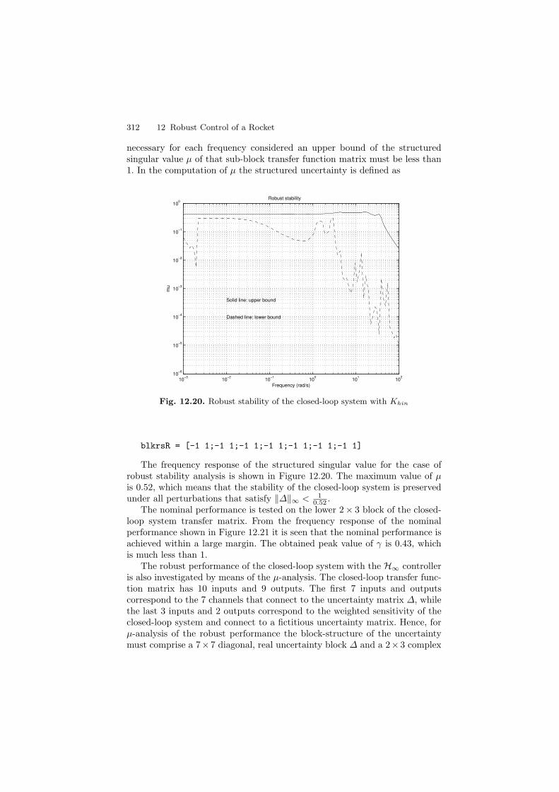
312 12 Robust Control of a Rocket
necessary for each frequency considered an upper bound of the structuredsingular value μ of that sub-block transfer function matrix must be less than1. In the computation of μ the structured uncertainty is defined as
10−3
10−2
10−1
100
101
102
10−6
10−5
10−4
10−3
10−2
10−1
100
Robust stability
Frequency (rad/s)
mu
Solid line: upper bound
Dashed line: lower bound
Fig. 12.20. Robust stability of the closed-loop system with Khin
blkrsR = [-1 1;-1 1;-1 1;-1 1;-1 1;-1 1;-1 1]
The frequency response of the structured singular value for the case ofrobust stability analysis is shown in Figure 12.20. The maximum value of μis 0.52, which means that the stability of the closed-loop system is preservedunder all perturbations that satisfy ‖Δ‖∞ < 1
0.52 .The nominal performance is tested on the lower 2× 3 block of the closed-
loop system transfer matrix. From the frequency response of the nominalperformance shown in Figure 12.21 it is seen that the nominal performance isachieved within a large margin. The obtained peak value of γ is 0.43, whichis much less than 1.
The robust performance of the closed-loop system with the H∞ controlleris also investigated by means of the μ-analysis. The closed-loop transfer func-tion matrix has 10 inputs and 9 outputs. The first 7 inputs and outputscorrespond to the 7 channels that connect to the uncertainty matrix Δ, whilethe last 3 inputs and 2 outputs correspond to the weighted sensitivity of theclosed-loop system and connect to a fictitious uncertainty matrix. Hence, forμ-analysis of the robust performance the block-structure of the uncertaintymust comprise a 7× 7 diagonal, real uncertainty block Δ and a 2× 3 complex

12.4 H∞ Design 313
10−3
10−2
10−1
100
101
102
0
0.05
0.1
0.15
0.2
0.25
0.3
0.35
0.4
0.45Nominal performance
Frequency (rad/s)
Fig. 12.21. Nominal performance of the closed-loop system for Khin
uncertainty block ΔF
ΔP :={[
Δ 00 ΔF
]: Δ ∈ R7×7, ΔF ∈ C2×3
}
The robust performance (with respect to the uncertainty and performanceweighting functions) is achieved if and only if, over a range of frequency underconsideration, the structured singular value μΔP
(jω) at each ω is less than 1.
The frequency response of μ for the case of robust performance analysisis given in Figure 12.22. The peak value of μ is 1.153, which shows that therobust performance has not been achieved. Or in other words, the system doesnot preserve performance under all relative parameter changes shown in Table12.3.
The results obtained are valid for t = 15 s. To check if the controllerdesigned achieves robust stability and robust performance of the closed-loopsystem at other time instants of flight, further analysis should be conductedwith corresponding dynamics.
The simulation of the closed-loop system is implemented by using thefile clp rock.m that corresponds to the structure shown in Figure 12.23. Inthis structure the performance weighting functions Wp and Wu, used in thesystem design and performance analysis, are absent. The simulation showsthe transient responses with respect to the reference signal for t = 15 s.The transient responses are computed by using the function trsp under theassumption of “frozen”model parameters. (Note that all transient responsesare shown with a time offset of 15 s.)
In Figure 12.24 we show the transient responses of the closed-loop systemwith the designed H∞ controller for a step signal with magnitude r = ±15g,

314 12 Robust Control of a Rocket
10−3
10−2
10−1
100
101
102
0
0.2
0.4
0.6
0.8
1
1.2
1.4Robust performance
Frequency (rad/s)
mu
Solid line: upper bound
Dashed line: lower bound
Fig. 12.22. Robust performance of the closed-loop system for Khin
Fig. 12.23. Structure of the closed-loop system

12.5 μ-Synthesis 315
0 1 2 3 4 5 6 7 8 9−25
−20
−15
−10
−5
0
5
10
15
20
25
Response in ny
Time (s)
n y (g)
Fig. 12.24. Transient response of the closed-loop system, t = 15 s
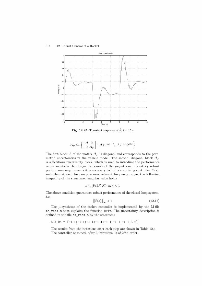
which corresponds to a change in the normal acceleration with ±15g. Thetransient response for this controller is oscillatory. The overshoot is under30% and the settling time is approximately 2 s. For the same reference signal,the transient response of the pitch rate θ is shown in Figure 12.25. The timeresponse contains high-frequency oscillations.
It is noticed that the H∞ controller designed does not satisfy the require-ments for the closed-loop system dynamics. Better results are obtained withthe μ-controller designed in the next section.
12.5 μ-Synthesis
In this section, we consider the same design problem but using another ap-proach, namely the μ-synthesis method. Because the uncertainties consideredin this case are highly structured, better results with respect to the closed-loopperformance may be achieved by the μ-synthesis.
The model of the open-loop system has 14 states, 11 inputs and 11 outputs.Uncertainties (i.e. parameter variations) are considered with seven parametersaΘΘ, aΘδz
, aθθ, aθθ, aθδz, anyα and anyδz
.Denote by P (s) the transfer function matrix of the 11-input, 11-output
open-loop system nominal dk and let the block structure of the uncertaintymatrix ΔP be defined as
316 12 Robust Control of a Rocket
0 1 2 3 4 5 6 7 8 9−1
−0.8
−0.6
−0.4
−0.2
0
0.2
0.4
0.6
0.8
1Response in dθ/dt
Time (s)
dθ/d
t (ra
d/s)
Fig. 12.25. Transient response of θ, t = 15 s
ΔP :={[
Δ 00 ΔF
]: Δ ∈ R7×7, ΔF ∈ C2×3
}
The first block Δ of the matrix ΔP is diagonal and corresponds to the para-metric uncertainties in the vehicle model. The second, diagonal block ΔF
is a fictitious uncertainty block, which is used to introduce the performancerequirements in the design framework of the μ-synthesis. To satisfy robustperformance requirements it is necessary to find a stabilising controller K(s),such that at each frequency ω over relevant frequency range, the followinginequality of the structured singular value holds
μΔP[FL(P, K)(jω)] < 1
The above condition guarantees robust performance of the closed-loop system,i.e.,
‖Φ(s)‖∞ < 1 (12.17)
The μ-synthesis of the rocket controller is implemented by the M-filems rock.m that exploits the function dkit. The uncertainty description isdefined in the file dk rock.m by the statement
BLK DK = [-1 1;-1 1;-1 1;-1 1;-1 1;-1 1;-1 1;3 2]
The results from the iterations after each step are shown in Table 12.4.The controller obtained, after 3 iterations, is of 28th order.

12.5 μ-Synthesis 317
Table 12.4. Results from the D-K iterations
Iteration Controller order Maximum value of μ
1 14 1.7302 18 1.0843 28 0.810
To check the robust stability and robust performance of the closed-loopsystem it is necessary to follow μ- analysis using again the file mu rock.m.
10−3
10−2
10−1
100
101
102
10−5
10−4
10−3
10−2
10−1
100
Robust stability
Frequency (rad/s)
mu
Solid line: upper bound
Dashed line: lower bound
Fig. 12.26. Robust stability of the closed-loop system with Kmu
The frequency response of the structured singular value for the case ofrobust stability is shown in Figure 12.26. The maximum value of μ is 0.441,which shows that under the considered parametric uncertainties the closed-loop system stability is preserved.
The frequency response of the structured singular value for the case ofrobust performance is shown in Figure 12.27. The maximum value of μ is0.852, which shows that the closed-loop system achieves robust performance.This value of μ is smaller than the corresponding value of μ, obtained in theH∞ design, i.e. the μ-controller provides better robustness.

318 12 Robust Control of a Rocket
10−3
10−2
10−1
100
101
102
0
0.1
0.2
0.3
0.4
0.5
0.6
0.7
0.8
0.9Robust performance
Frequency (rad/s)
mu
Solid line: upper bound
Dashed line: lower bound
Fig. 12.27. Robust performance of the closed-loop system with Kmu
10−1
100
101
102
103
−100
−80
−60
−40
−20
0
20
Frequency (rad/s)
Mag
nitu
de (
dB)
Closed−loop magnitude plot
Fig. 12.28. Magnitude response of the closed-loop system
The frequency responses of the closed-loop system with the μ-controllerare obtained by using the file frs rock.m and are shown in Figures 12.28 and12.29. Over the low-frequency region the value of the magnitude response is

12.5 μ-Synthesis 319
10−1
100
101
102
103
−250
−200
−150
−100
−50
0
Frequency (rad/s)
Pha
se (
deg)
Closed−loop phase plot
Fig. 12.29. Phase response of the closed-loop system
close to 1, i.e. the reference signal can be followed accurately. The closed loopsystem bandwidth is about 2 rad/s.
10−1
100
101
102
103
104
−160
−140
−120
−100
−80
−60
−40
Frequency (rad/s)
Mag
nitu
de (
dB)
Sensitivity to accelerometer and rate gyro noises
Solid line: sensitivity to accelerometer noise
Dashed line: sensitivity to rate gyro noise
Fig. 12.30. Sensitivity to the noises ηa and ηg

320 12 Robust Control of a Rocket
In Figure 12.30 we show the frequency responses of the transfer functionswith respect to the noises ηa and ηg. The noises of the accelerometer andof the rate gyro are attenuated 1000 times (60 dB), i.e. both noises have arelatively weak influence on the output of the closed-loop system.
10−1
100
101
102
103
104
−80
−60
−40
−20
0
20
40
60
Frequency (rad/s)
Mag
nitu
de (
dB)
Controller magnitude plot
Solid line: Kδ
o n
y
Dashed line: Kδ
o dθ/dt
Fig. 12.31. Controller magnitude plots
The magnitude and phase plots of the controller transfer functions areshown in Figures 12.31 and 12.32, respectively.
In Figure 12.33 we show the transient responses of the closed-loop systemwith the designed μ-controller for a step signal with magnitude
r = ±15 g
that corresponds to a change in the normal acceleration with ±15g. The over-shoot is under 1% and the settling time is less than 1 s. For the same referencesignal, the transient response of the pitch rate θ is shown in Figure 12.34.
The angle of deflation δz of the control fins in the closed loop system isshown in Figure 12.35. The magnitude of this angle is less than 30 deg, asrequired. In Figure 12.36 we show the perturbed transient responses of theclosed-loop system for a step reference signal with magnitude r = ±15g.
The designed μ-controller can be used in cases of a wider range of vehiclecoefficient values. In Figure 12.37 we show the transient response with respectto the reference signal for the 15th second of the flight at altitude H = 1000 m

12.5 μ-Synthesis 321
10−1
100
101
102
103
104
−200
−150
−100
−50
0
50
100
150
200
Frequency (rad/s)
Pha
se (
deg)
Controller phase plot
Solid line: Kδ
o n
y
Dashed line: Kδ
o dθ/dt
Fig. 12.32. Controller phase plots
0 1 2 3 4 5 6 7 8 9−20
−15
−10
−5
0
5
10
15
20
Response in ny
Time (s)
n y (g)
Fig. 12.33. Transient response of the closed loop system, t = 15 s
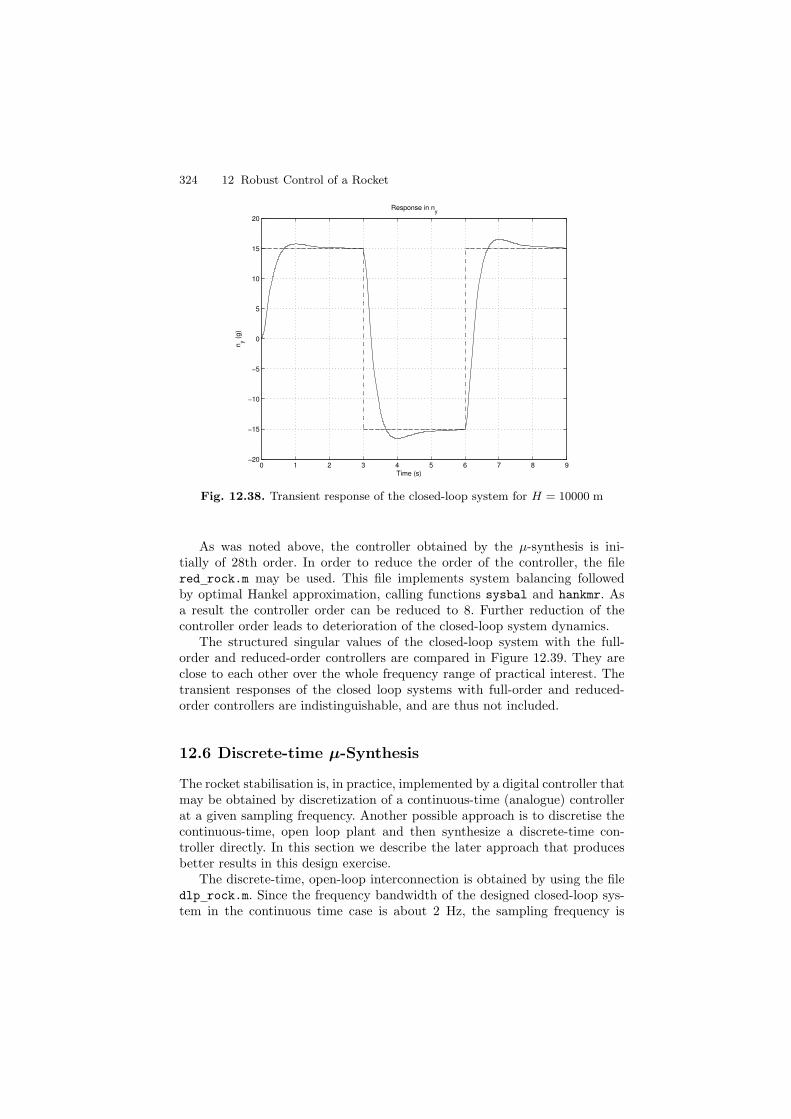
and in Figure 12.38 is the corresponding transient response for the 15th secondof the flight at altitude H = 10000 m. Due to the achieved robustness of theclosed-loop system, both responses are similar to that of the design case,

322 12 Robust Control of a Rocket
0 1 2 3 4 5 6 7 8 9−0.8
−0.6
−0.4
−0.2
0
0.2
0.4
0.6
0.8Response in dϑ/dt
Time (s)
dϑ/d
t (ra
d/s)
Fig. 12.34. Transient response of θ, t = 15 s
0 1 2 3 4 5 6 7 8 9−0.4
−0.3
−0.2
−0.1
0
0.1
0.2
0.3
0.4Fin deflection
Time (s)
δ (
rad)
Fig. 12.35. Control action in the closed loop system, t = 15 s
though there is significant difference in the rocket dynamics between thesetwo cases and the design case. This shows that the designed controller may be

12.5 μ-Synthesis 323
0 1 2 3 4 5 6 7 8 9−20
−15
−10
−5
0
5
10
15
20Transient responses of the perturbed systems
Time (s)
n y (g)
Fig. 12.36. Perturbed transient response of the closed-loop system, t = 15 s
0 1 2 3 4 5 6 7 8 9−15
−10
−5
0
5
10
15
Response in ny
Time (s)
n y (g)
Fig. 12.37. Transient response of the closed-loop system for H = 1000 m
employed for system stabilisation for different altitudes and velocities, whichwould simplify the controller implementation.
324 12 Robust Control of a Rocket
0 1 2 3 4 5 6 7 8 9−20
−15
−10
−5
0
5
10
15
20
Response in ny
Time (s)
n y (g)
Fig. 12.38. Transient response of the closed-loop system for H = 10000 m
As was noted above, the controller obtained by the μ-synthesis is ini-tially of 28th order. In order to reduce the order of the controller, the filered rock.m may be used. This file implements system balancing followedby optimal Hankel approximation, calling functions sysbal and hankmr. Asa result the controller order can be reduced to 8. Further reduction of thecontroller order leads to deterioration of the closed-loop system dynamics.
The structured singular values of the closed-loop system with the full-order and reduced-order controllers are compared in Figure 12.39. They areclose to each other over the whole frequency range of practical interest. Thetransient responses of the closed loop systems with full-order and reduced-order controllers are indistinguishable, and are thus not included.
12.6 Discrete-time μ-Synthesis
The rocket stabilisation is, in practice, implemented by a digital controller thatmay be obtained by discretization of a continuous-time (analogue) controllerat a given sampling frequency. Another possible approach is to discretise thecontinuous-time, open loop plant and then synthesize a discrete-time con-troller directly. In this section we describe the later approach that producesbetter results in this design exercise.
The discrete-time, open-loop interconnection is obtained by using the filedlp rock.m. Since the frequency bandwidth of the designed closed-loop sys-tem in the continuous time case is about 2 Hz, the sampling frequency is

12.6 Discrete-time μ-Synthesis 325
10−6
10−4
10−2
100
102
104
10−2
10−1
100
101
102
103
Singular values of the controller transfer function matrices
Frequency (rad/s)
Solid line: full−order controller
Dashed line: reduced−order controller
Fig. 12.39. Singular values of the full-order controller and reduced-order controller
chosen equal to 250 Hz that corresponds to a sampling period Ts of 0.004 s.For this frequency we derive a discretised model of the open-loop system byusing the function samhld. The controller may be synthesised by the aid ei-ther of H∞ optimisation (by using the function dhinfsyn), or μ-synthesis (byusing the function dkit). In the following, we consider the μ-synthesis of adiscrete-time controller that is obtained by implementing the files dms rock.mand ddk rock.m.
As in the μ-synthesis of the continuous-time controller, the synthesis isconducted for the full-order vehicle model. Hence, the uncertainty structureunder consideration is of the form
BLK DK = [-1 1;-1 1;-1 1;-1 1;-1 1;-1 1;-1 1;3 2]
In the discrete-time case, the frequency range is on the unit circle andchosen as the interval [0, π]. To set up 100 frequencies, the following line isused
OMEGA DK = [pi/100:pi/100:pi];
For the discrete-time design it is necessary to include the command line
DISCRETE DK = 1;

326 12 Robust Control of a Rocket
The design follows the usual route, by calling the function dkit. In Table12.5 the results of the discrete time D-K iterations are listed.
Table 12.5. Results of the D-K iterations
Iteration Controller order Maximum value of μ
1 14 2.1012 22 0.6003 28 0.730
The discrete-time controller KD obtained is of 28th order. Note that betterrobustness is achieved with the controller obtained at the 2nd step. Thiscontroller, however, does not ensure the desired closed-loop dynamics.
10−3
10−2
10−1
100
101
102
103
10−7
10−6
10−5
10−4
10−3
10−2
10−1
100
Robust stability
Frequency (rad/s)
mu Solid line: upper bound
Dashed line: lower bound
Fig. 12.40. Robust stability of the closed-loop system with KD
Robust stability and robust performance of the closed-loop system withKD are shown in Figures 12.40 and 12.41, respectively, in which the μ valuesover frequency range are calculated by the file dmu rock.m. It is seen that thediscrete-time closed-loop system achieves both robust stability and robustperformance, just as in the continuous-time case with Kmu.

12.6 Discrete-time μ-Synthesis 327
10−3
10−2
10−1
100
101
102
103
0
0.1
0.2
0.3
0.4
0.5
0.6
0.7
0.8
0.9Robust performance
Frequency (rad/s)
mu
Solid line: upper bound
Dashed line: lower bound
Fig. 12.41. Robust performance of the closed-loop system with KD
0 1 2 3 4 5 6 7 8 9−20
−15
−10
−5
0
5
10
15
20
Response in ny
Time (s)
n y (g)
Fig. 12.42. Transient response for KD, t = 15 s

328 12 Robust Control of a Rocket
0 1 2 3 4 5 6 7 8 9−0.4
−0.3
−0.2
−0.1
0
0.1
0.2
0.3
0.4Fin deflection
Time (s)
δ (
rad)
Fig. 12.43. Control action in the closed loop system for KD, t = 15 s
In Figures 12.42 and 12.43 we show the transient response of the closedloop system with respect to the reference signal, and the corresponding controlaction, respectively. These two figures are generated by the file dcl rock.mthat utilises the function sdtrsp.
The results displayed above show that the achieved behaviour of the sam-pled data, closed-loop system are close to those in the continuous-time case,with each corresponding μ-controller.
12.7 Simulation of the Nonlinear System
The dynamics of the nonlinear, time-varying rocket model differs from thatof the linear, time-invariant model used in the analysis and design describedin the previous sections. Also, for large reference signals there is a stronginterconnection between the longitudinal and lateral motions that may affectthe stability and performance of the whole system. It is therefore importantto study the dynamic behaviour of the closed loop, nonlinear, time-varyingsystem with the designed controller that regulates the six-degree-of-freedomrocket motion.
The closed-loop rocket stabilisation system of the nonlinear, time-varyingplant is simulated by using the Simulink r© models c rock.mdl (for thecontinuous-time system with an analogue controller) as well as d rock.mdl(for the sampled data system with a digital controller). Both systems involve

12.7 Simulation of the Nonlinear System 329
two identical controllers for the longitudinal and lateral motion. The sampled-data system also contains 16-bit analogue-to-digital and digital-to-analogueconverters. (The outputs of the digital-to-analogue converters are scaled togive the reference input of the servo-actuators.) Both models allow us to sim-ulate the closed-loop system for different reference, disturbance and noisesignals. The roll motion is stabilised by a separate gyro with simple lead-lagcompensator. (A robust roll controller is also possible to implement.)
In Figure 12.44 we show the Simulink r© model d rock.mdl of the nonlin-ear, sampled-data, closed-loop system.
Before carrying out simulation it is necessary to assign the model param-eters by using the M-file init c rock.m (in the continuous-time case) or thethe M-file init d rock.m (in the discrete-time case).
Before the perturbation motion begins to affect (i.e. before the time in-stance t0), only the nonlinear equations of the unperturbed (program) motionare solved. (This ensures that the parameters of the linearised model at t0are the same as those used in the controller design.) After t0, the equationsof the perturbed motions are solved by using the S-function s rock.m. Theinitial conditions for the perturbed motion are assigned in the file inc rock.mthat is invoked by s rock.m. During the time interval [0, t0], the equationsof the unperturbed motion are solved in the file inc rock.m by using thefunction sol rock.m. The values of the pitch angle θ for the program motionare assigned in the file theta rock.m.
The simulation of the perturbed motion, which involves the controlleraction, is based on the nonlinear differential and algebraic equations (12.1)–(12.5).
In Figures 12.45 and 12.46 we show the transient response of the nonlinearsampled-data system with respect to the normal accelerations ny and nz,respectively, for a reference step change of 15g occurring at t0 = 15 s in eachchannel. In the simulation we used the discrete-time controller designed for thesame moment of the time in the previous section. It is seen that the behaviourof nz is very close to the behaviour of the corresponding variable shown inFigure 12.42. The small difference in the responses of ny and nz is due to theinfluence of the Earth’s gravity on the pitch angle.

330 12 Robust Control of a Rocket
Sim
ulin
k m
odel
of
the
sam
pled
−dat
a ro
cket
sta
bilis
atio
n sy
stem
y
n_z
n_y
om_z
om_y
Pit
ch c
ontr
ol
Yaw
con
trol
Rol
l con
trol
gam
ma
Gai
n2
ref_
nz
ref_
nyom
ega_
z
omeg
a_y
n_z
n_y
gam
ma
delta
_z
delta
_y
t
Tim
e
Sat
urat
ion2
Sat
urat
ion1
ainW
i*nu
mW
i(s)
denW
i(s)
Rol
l giro
ainW
r*nu
mW
r(s
denW
r(s)
Rol
l fin
s
num
(s)
denK
r(s)
Rol
l com
pens
ator
s_ro
ck
Roc
ket ai
nWg*
num
Wg(
s
denW
g(s)
Rat
e gi
ro_z
ainW
g*nu
mW
g(s
denW
g(s)
Rat
e gi
ro_y
y
Out
puts
6_13
n_z
Out
put5
n_y
Out
put4
Out
1
Out
2
Out
3
Out
4
Noi
se
−1
Gai
n4−1
Gai
n3
Ka
Ka
Gai
n1
ainW
d*nu
mW
d(s
denW
d(s)
Fin
s_z
ainW
d*nu
mW
d(s
denW
d(s)
Fin
s_y
em
In1
Out
1
Con
trol
ler_
z
In1
Out
1
Con
trol
ler_
y
Clo
ck
ainW
a*nu
mW
a(s
denW
a(s)
Acc
eler
omet
er_z
ainW
a*nu
mW
a(s
denW
a(s)
Acc
eler
omet
er_y
Fig. 12.44. Simulation model of the nonlinear sampled data system

12.7 Simulation of the Nonlinear System 331
14 15 16 17 18 19 20−2
0
2
4
6
8
10
12
14
16
Time (s)
n y (g)
Nonlinear response in ny
Fig. 12.45. Transient responses in ny of the nonlinear sampled-data system
14 15 16 17 18 19 20−2
0
2
4
6
8
10
12
14
16
Time (s)
n z (g)
Nonlinear response in nz
Fig. 12.46. Transient responses in nz of the nonlinear sampled-data system

332 12 Robust Control of a Rocket
12.8 Conclusions
From the results/experiences obtained, the design of a robust stabilisationsystem for a winged, supersonic rocket may be summarised as the following.
• The linearised equations of the rocket should be arranged in a properway in order to avoid the appearance of an additional integrator in theuncertainty model. The inclusion of this integrator leads to violation ofthe conditions for H∞ design.
• Both H∞ optimisation and μ-synthesis approaches may be used to designcontrollers that, for a specified moment of flight dynamics, achieve robuststability of the rocket stabilisation system in the presence of disturbancesand sensor noises. However, the H∞ controller can not ensure robust per-formance in the given case. The μ-controller achieves both robust stabilityand robust performance of the closed-loop system.
• The μ-controller obtained may be used successfully for different altitudesand Mach numbers. However, in order to control the rocket efficientlythrough the whole flight envelope it may be necessary to implement severalcontrollers designed for different flight conditions.
• A digital controller has been successfully designed for a discrete-time modelof the open-loop system. The corresponding sampled data, closed-loopsystem achieves robust stability and robust performance at almost thesame as the continuous-time one.
• The μ-synthesis in the discrete-time case shows that achieving a smallervalue of μ may lead to the deterioration of the system dynamics, i.e. betterrobustness may be achieved at the price of poorer dynamics. This is whya value of μ slightly less than 1 may be a good trade-off between therequirements for the robustness and dynamic performance.
• The simulation of the nonlinear, time-varying closed-loop system showsthat for a sufficiently large interval of time, the dynamics behaviour is closeto that of the time-invariant system which has fixed model parameters.
Notes and References
The design of rocket and spacecraft flight-control systems is considered indepth in many books, see for example [11, 12, 54, 172]. The design of robustflight-control systems is presented in [7, 36]. Ensuring good performance ofthe closed-loop system for the whole range of the flight operating conditionsby a fixed controller is rarely possible and, in general, it is necessary to changethe controller parameters as the rocket model varies. For this aim, it is possi-ble to use some technique of gain scheduling: see the survey papers [84, 131].The classical approach for gain scheduling is to design several time-invariantcontrollers for different points in the operational region and then interpolatetheir parameters for the intermediate values, see, for instance, [130, 118, 13].

12.8 Conclusions 333
This approach has several disadvantages, for instance it is difficult to guar-antee robust stability and robust performance in the transition regions, i.e.between design points at which the controllers are designed. In this respectrobust controllers are more suitable for gain scheduling since they ensure sat-isfactory performance at least in some neighbourhood around an operatingpoint and thus fewer fixed controllers are needed. Another approach for gainscheduling is to derive a linear, parameter-varying(LPV) model of the rocketand then design an LPV controller that hopefully will achieve the desiredperformance for the whole range of operating conditions. Examples of usingthis approach may be found in [37, 143].
The elasticity of the rocket body may affect significantly the dynamics ofthe closed-loop system, see, for instance, [11, 91].


![Robust Model Predictive Control - Carnegie Mellon …cepac.cheme.cmu.edu/.../Ronust_Control_Classnotes.pdf1 Robust Model Predictive Control Formulations of robust control [1] The robust](https://img.dokumen.tips/doc/110x75/5aab45707f8b9a2b4c8bd345/robust-model-predictive-control-carnegie-mellon-cepacchemecmueduronustcontrol.jpg)