12-1

Chapter

Twelve

McGraw-Hill/Irwin

© 2006 The McGraw-Hill Companies, Inc., All Rights Reserved.

12-2

Chapter TwelveAnalysis of VarianceAnalysis of Variance

GOALSWhen you have completed this chapter, you will be able to:

ONE List the characteristics of the F distribution.

TWOConduct a test of hypothesis to determine whether the variances of two populations are equal.

THREEDiscuss the general idea of analysis of variance.

Goals

12-3

Chapter Twelve continuedAnalysis of VarianceAnalysis of Variance

GOALSWhen you have completed this chapter, you will be able to:FOUROrganize data into a one-way and a two-way ANOVA table.FIVE Conduct a test of hypothesis among three or more treatment means.

SIXDevelop confidence intervals for the difference between treatment means.

Goals

12-4

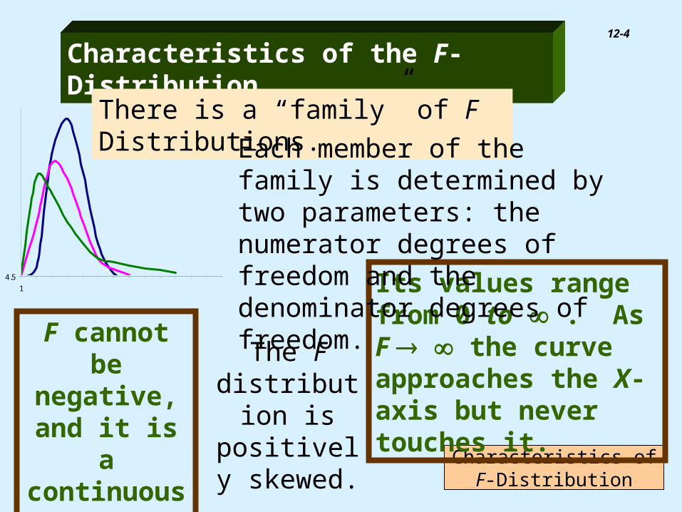
Characteristics of F-Distribution

Its values range from 0 to . As F the curve approaches the X-axis but never touches it.

Characteristics of the F-Distribution

There is a “family” of F Distributions.

Each member of the family is determined by two parameters: the numerator degrees of freedom and the denominator degrees of freedom.

F cannot be negative, and

it is a continuous

distribution.

The F distribution is

positively skewed.

4.5

1

12-5

Test for Equal Variances of Two Populations

22

21

s

sF

22s

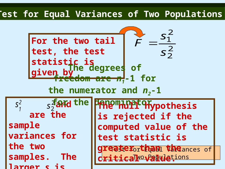
For the two tail test, the test statistic is given by

Test for Equal Variances of Two Populations

and are the sample variances for the two samples. The larger s is placed in the denominator.

s 21

The degrees of freedom are n1-1 for the numerator and n2-1 for the denominator.

The null hypothesis is rejected if the computed value of the test statistic is greater than the critical value.

12-6

Example 1

The mean rate of return on a sample of 8 utility stocks was 10.9 percent with a standard deviation of 3.5 percent. At the .05 significance level, can Colin conclude that there is more variation in the software stocks?

Colin, a stockbroker at Critical Securities, reported that the mean rate of return on a sample of 10 internet stocks was 12.6 percent with a standard deviation of 3.9 percent.

12-7

Example 1 continued

221

220

:

:

UI

UI

H

H

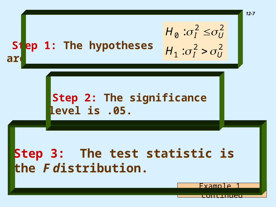
Step 3: The test statistic is the F distribution.

Step 1: The hypotheses are

Step 2: The significance level is .05.

12-8

Example 1 continued

2416.1)5.3(

)9.3(2

2

F

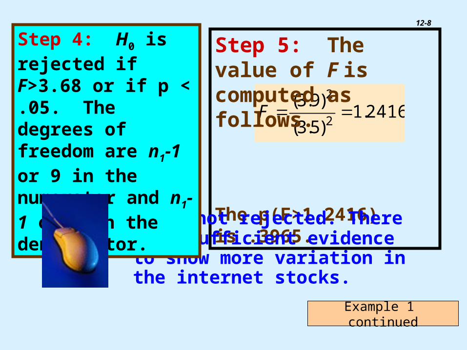
Step 5: The value of F is computed as follows.

The p(F>1.2416) is .3965.

H0 is not rejected. There is insufficient evidence to show more variation in the internet stocks.

Step 4: H0 is rejected if F>3.68 or if p < .05. The degrees of freedom are n1-1 or 9 in the numerator and n1-1 or 7 in the denominator.

12-9

The ANOVA Test of Means

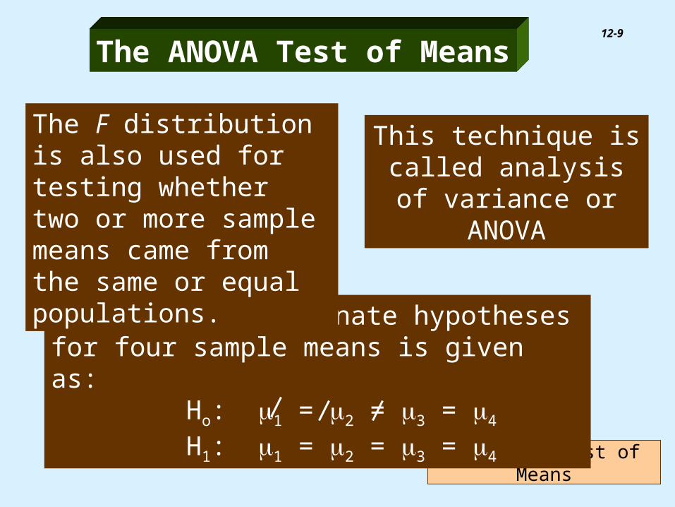
The null and alternate hypotheses for four sample means is given as:

Ho: 1 = 2 = 3 = 4 H1: 1 = 2 = 3 = 4

The ANOVA Test of Means

The F distribution is also used for testing whether two or more sample means came from the same or equal populations.

This technique is called analysis of variance or

ANOVA

12-10

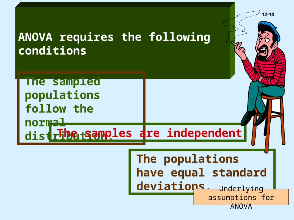
The populations have equal standard deviations.

ANOVA requires the following conditions

Underlying assumptions for ANOVA

The sampled populations follow the normal distribution.

The samples are independent

12-11

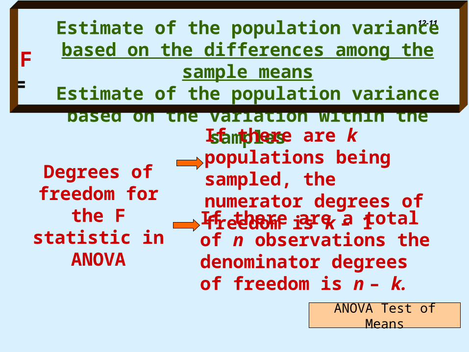
F =

Estimate of the population variancebased on the differences among the sample means

Estimate of the population variancebased on the variation within the samples

ANOVA Test of Means

Degrees of freedom for the F statistic in

ANOVA

If there are k populations being sampled, the numerator degrees of freedom is k – 1

If there are a total of n observations the denominator degrees of freedom is n – k.

12-12

In the following table, i stands for the ith observationc stands for cth treatment groupxG is the overall or grand mean k is the number of treatment groups

ANOVA Test of Means

ANOVA divides the Total VariationTotal Variation into the

variation due to the treatment, Treatment VariationTreatment Variation,

and to the error component, Random VariationRandom Variation.

12-13

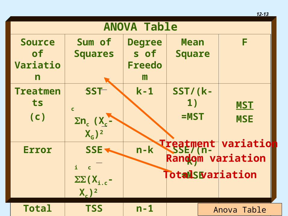
ANOVA TableSource of Variation

Sum of Squares

Degrees of

Freedom

Mean Square

F

Treatments

(c)

SST

c

nc (Xc-XG)2

k-1 SST/(k-1)

=MST MST

MSE

Error SSE

i c

(Xi.c-Xc)2

n-k SSE/(n-k)

=MSE

Total TSS

i

(Xi-XG)2

n-1

Anova Table

Treatment variation

Random variation

Total variation

12-14

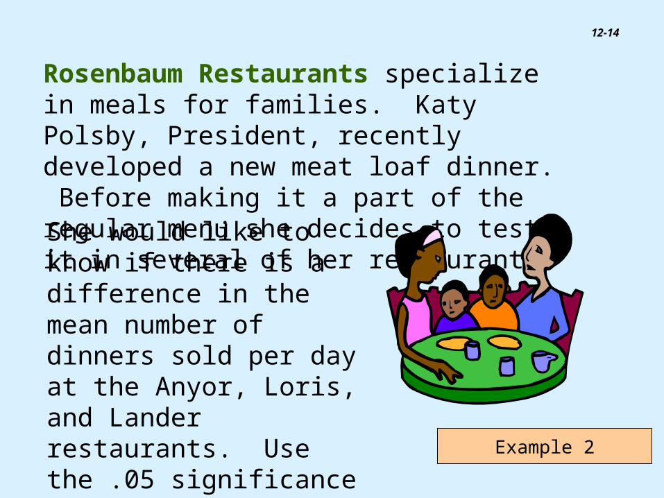
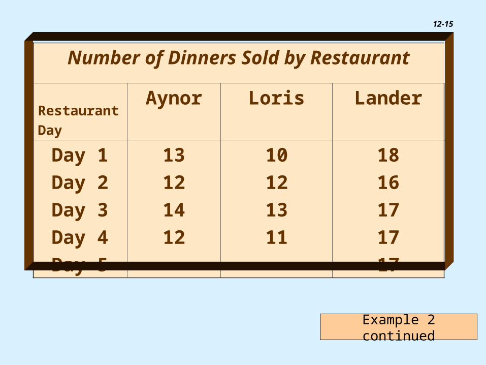
Rosenbaum Restaurants specialize in meals for families. Katy Polsby, President, recently developed a new meat loaf dinner. Before making it a part of the regular menu she decides to test it in several of her restaurants.

Example 2

She would like to know if there is a difference in the mean number of dinners sold per day at the Anyor, Loris, and Lander restaurants. Use the .05 significance level.

12-15

Number of Dinners Sold by Restaurant

Restaurant

DayAynor Loris Lander

Day 1

Day 2

Day 3

Day 4

Day 5

13

12

14

12

10

12

13

11

18

16

17

17

17

Example 2 continued

12-16

Step One: State the null hypothesis and the alternate hypothesis.

Ho: Aynor = Loris = Landis H1: Aynor = Loris = Landis

Step Two: Select the level of significance. This is given in the problem statement as .05.

Step Three: Determine the test statistic. The test statistic follows the F distribution.

Example 2 continued

12-17

Step Five: Select the sample, perform the calculations, and make a decision.

Step Four: Formulate the decision rule.The numerator degrees of freedom, k-1, equal 3-1 or 2. The denominator degrees of freedom, n-k, equal 13-3 or 10. The value of F at 2 and 10 degrees of freedom is 4.10. Thus, H0 is rejected if F>4.10 or p< of .05.

Example 2 continued

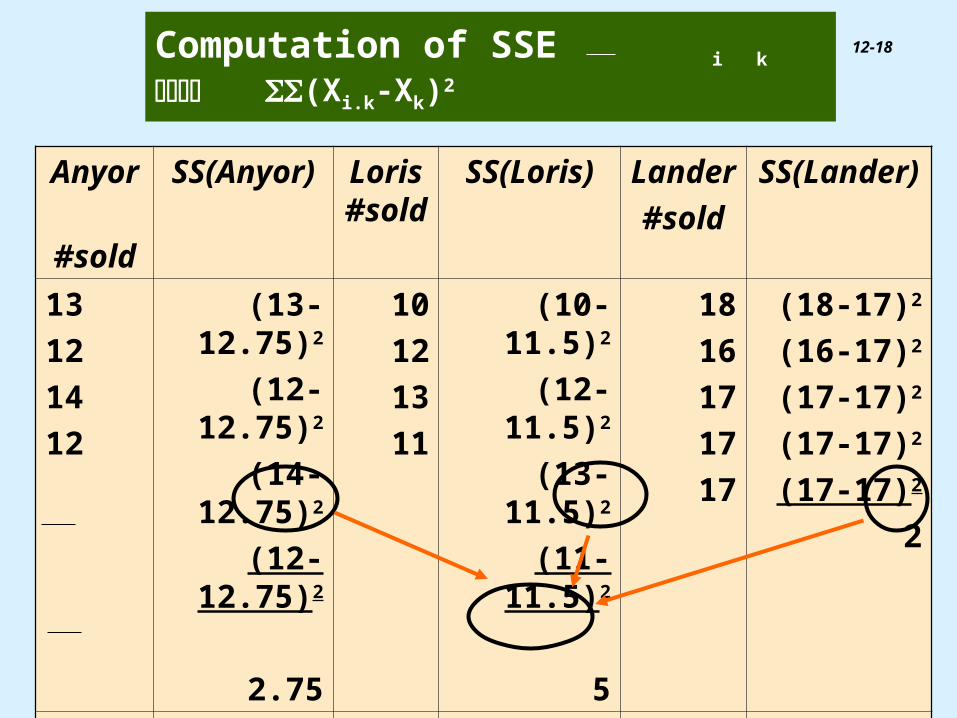
Using the data provided, the ANOVA calculations follow.

12-18

Anyor

#sold

SS(Anyor) Loris #sold

SS(Loris) Lander

#sold

SS(Lander)

13

12

14

12

(13-12.75)2

(12-12.75)2

(14-12.75)2

(12-12.75)2

2.75

10

12

13

11

(10-11.5)2

(12-11.5)2

(13-11.5)2

(11-11.5)2

5

18

16

17

17

17

(18-17)2

(16-17)2

(17-17)2

(17-17)2

(17-17)2

2

Xk 12.75 11.5 17

SSE: 2.75 + 5 + 2 = 9.75

XG: 14.00

Computation of SSE i k

(Xi.k-Xk)2

12-19

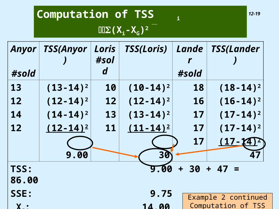
Anyor

#sold

TSS(Anyor) Loris #sold

TSS(Loris) Lander

#sold

TSS(Lander)

13

12

14

12

(13-14)2

(12-14)2

(14-14)2

(12-14)2

9.00

10

12

13

11

(10-14)2

(12-14)2

(13-14)2

(11-14)2

30

18

16

17

17

17

(18-14)2

(16-14)2

(17-14)2

(17-14)2

(17-14)2

47

TSS: 9.00 + 30 + 47 = 86.00

SSE: 9.75

XG: 14.00

Computation of TSS i

(Xi-XG)2

Example 2 continued Computation of TSS

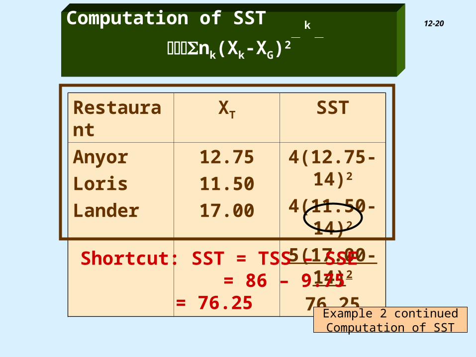
12-20Computation of SST k

nk(Xk-XG)2

Restaurant XT SST

Anyor

Loris

Lander

12.75

11.50

17.00

4(12.75-14)2

4(11.50-14)2

5(17.00-14)2

76.25

Shortcut: SST = TSS – SSE = 86 – 9.75

= 76.25Example 2 continued Computation of SST

12-21

ANOVA TableSource of Variation

Sum of Squares

Degrees of

Freedom

Mean Square

F

Treatments 76.25 3-1

=2

76.25/2

=38.125 38.125

.975

= 39.103

Error 9.75 13-3

=10

9.75/10

=.975

Total 86.00 13-1

=12

Example 2 continued

12-22

Example 2 continued

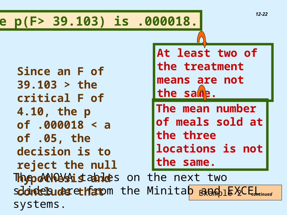
The ANOVA tables on the next two slides are from the Minitab and EXCEL systems.

The p(F> 39.103) is .000018.

The mean number of meals sold at the three locations is not the same.

Since an F of 39.103 > the critical F of 4.10, the p of .000018 < a of .05, the decision is to reject the null hypothesis and conclude that

At least two of the treatment means are not the same.

12-23

Example 2 continued

Analysis of Variance

Source DF SS MS F P

Factor 2 76.250 38.125 39.10 0.000

Error 10 9.750 0.975

Total 12 86.000

Individual 95% CIs For Mean

Based on Pooled StDev

Level N Mean StDev ---------+---------+---------+-------

Aynor 4 12.750 0.957 (---*---)

Loris 4 11.500 1.291 (---*---)

Lander 5 17.000 0.707 (---*---)

---------+---------+---------+-------

Pooled StDev = 0.987 12.5 15.0 17.5

12-24

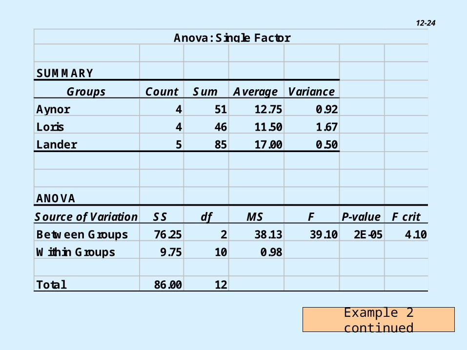
SUMMARY

Groups Count Sum Average Variance

Aynor 4 51 12.75 0.92

Loris 4 46 11.50 1.67

Lander 5 85 17.00 0.50

ANOVA

Source of Variation SS df MS F P-value F crit

Between Groups 76.25 2 38.13 39.10 2E-05 4.10

Within Groups 9.75 10 0.98

Total 86.00 12

Anova: Single Factor

Example 2 continued

12-25

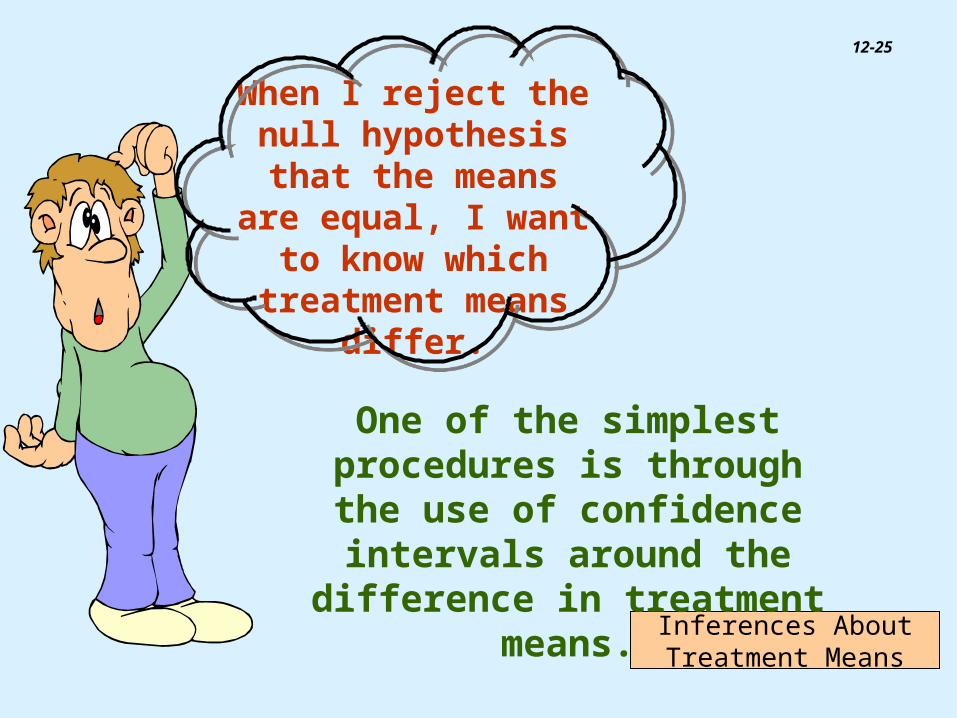
Inferences About Treatment Means

One of the simplest procedures is through the use of confidence intervals around the difference

in treatment means.

When I reject the null hypothesis that the

means are equal, I want to know which

treatment means differ.

12-26

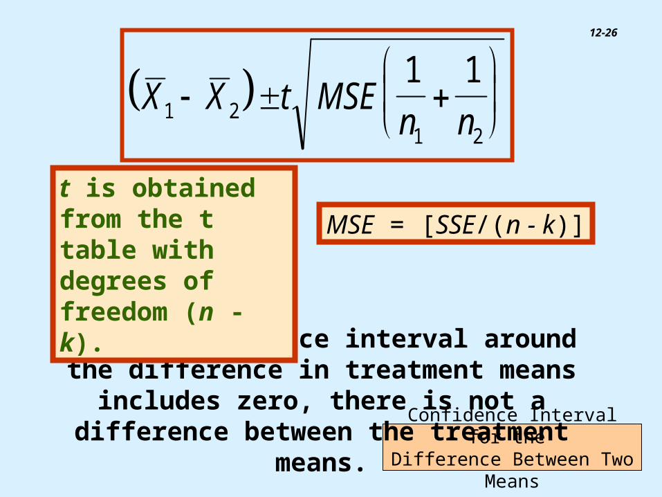
Confidence Interval for the Difference Between Two Means

X X t MSEn n1 2

1 2

1 1

If the confidence interval around the difference in treatment means includes zero, there is not a

difference between the treatment means.

t is obtained from the t table with degrees of freedom (n - k).

MSE = [SSE/(n - k)]

12-27

EXAMPLE 3

( . ) . .

. . ( . , . )

17 12 75 2 228 9751

4

1

5

4 25 148 2 77 5 73

95% confidence interval for the difference in the mean number of meat loaf dinners sold in Lander and Aynor

Can Katy conclude that there is a difference between the two restaurants?

12-28

Example 3continued

The mean number of meals sold in

Aynor is different from Lander.

Because zero is not in the interval, we conclude that this

pair of means differs.